YITP-17-47

OU-HET 933


Refined geometric transition and qq𝑞𝑞qq-characters
Taro Kimura***taro.kimura@keio.jp, Hironori Morihironori.mori@yukawa.kyoto-u.ac.jp, and Yuji Sugimotosugimoto@het.phys.sci.osaka-u.ac.jp


Department of Physics, Keio University, Kanagawa 223-8521, Japan
Fields, Gravity & Strings, CTPU, Institute for Basic Science, Daejeon 34047, Korea


Yukawa Institute for Theoretical Physics, Kyoto University, Kyoto 606-8502, Japan


Department of Physics, Graduate School of Science, Osaka University,
Toyonaka, Osaka 560-0043, Japan


Abstract

We show the refinement of the prescription for the geometric transition in the refined topological string theory and, as its application, discuss a possibility to describe qq𝑞𝑞qq-characters from the string theory point of view. Though the suggested way to operate the refined geometric transition has passed through several checks, it is additionally found in this paper that the presence of the preferred direction brings a nontrivial effect. We provide the modified formula involving this point. We then apply our prescription of the refined geometric transition to proposing the stringy description of doubly quantized Seiberg–Witten curves called qq𝑞𝑞qq-characters in certain cases.

1 Introduction

We have encountered the great developments of exact methods and a variety of their applications in quantum field theory, for instance, the Seiberg–Witten theory [1, 2] and the Nekrasov partition function for instanton counting problem [3, 4] as prominent landmarks, which are part of subjects in this paper. Correspondingly, the string theory and M-theory realization of these ingredients have been established and passed through a pile of checks in literatures. Specifically, (the 5d uplift of) the Nekrasov partition function can be systematically obtained by using the topological vertex [5] that is a powerful ingredient to calculate the amplitude in the topological string theory [6, 7, 8, 9] for a given Calabi–Yau threefold as the target space. The free energy of the topological string amplitude is expanded standardly with respect to the genus and the string coupling constant. The latter is translated into the ΩΩ\Omega-backgrounds (ϵ1,ϵ2)subscriptitalic-ϵ1subscriptitalic-ϵ2(\epsilon_{1},\epsilon_{2}) in a special limit ϵ1+ϵ2=0subscriptitalic-ϵ1subscriptitalic-ϵ20\epsilon_{1}+\epsilon_{2}=0 which is called the unrefined (self-dual) limit. Since the Nekrasov partition function could be actually formulated for a general value of (ϵ1,ϵ2)subscriptitalic-ϵ1subscriptitalic-ϵ2(\epsilon_{1},\epsilon_{2}), the refined version of the topological vertex to include two parameters given by

q1=e2πiϵ1,q2=e2πiϵ2formulae-sequencesubscript𝑞1superscript𝑒2𝜋isubscriptitalic-ϵ1subscript𝑞2superscript𝑒2𝜋isubscriptitalic-ϵ2\displaystyle q_{1}=e^{2\pi\mathrm{i}\epsilon_{1}},\hskip 20.00003ptq_{2}=e^{2\pi\mathrm{i}\epsilon_{2}} (1.1)

has been suggested by [10, 11], which was named the refined topological vertex111The convention here is translated into (q,t)𝑞𝑡(q,t) for the ΩΩ\Omega-backgrounds used in [11] as (q,t1)(q1,q2)𝑞superscript𝑡1subscript𝑞1subscript𝑞2(q,t^{-1})\to(q_{1},q_{2}).. Their definition could successfully reproduce the Nekrasov partition function with general ΩΩ\Omega-background in many circumstances and bring us to meaningful outcomes from string theory to supersymmetric gauge theories (basically with eight supercharges).

It has been shown in [12, 13, 14] that the open string and closed string sector in the usual (i.e. unrefined) topological sting theory is just linked by the geometric transition (open/closed duality). However, underlying physics for the geometric transition in the refined topological string theory that we would refer to as the refined geometric transition is not yet well understood mainly because there is no known world-sheet interpretation of it. Recently, great quantitative support for the refined geometric transition was reported by [15].

The prescription for geometric transition in terms of the refined topological vertex has been proposed [16] and basically checked in the context of the AGT correspondence [17, 18], but it is not complete due to the possible choice of the so-called the preferred direction on the refined topological vertex. The topological vertex is graphically a trivalent vertex, and the proper point of the refined vertex different from the unrefined one is the existence of the preferred direction that is a special direction out of three edges of the vertex. This does result from the inclusion of (q1,q2)subscript𝑞1subscript𝑞2(q_{1},q_{2}) into the topological vertex. It is labeled by a Young diagram assigned on each edge, and as well, we pick up two of three edges to put (q1,q2)subscript𝑞1subscript𝑞2(q_{1},q_{2}) on. This means that the the preferred direction as the last edge has a special role on the computation of the refined topological string amplitude. In the first half of the paper, it will be argued that the refined geometric transition has to be sensitive to the choice of the preferred direction, and we will provide another prescription to implement the refined geometric transition on the web diagram constructed by vertices with the preferred direction that differs from the conventional one mentioned above.

In order to check the consistency of our prescription, we explore double quantization of the Seiberg–Witten geometry, which is called the qq𝑞𝑞qq-character, by utilizing the refined geometric transition. The qq𝑞𝑞qq-character has been recently introduced by Nekrasov in the context of the BPS/CFT correspondence [19, 20, 21]. It is a natural gauge theoretical generalization of the q𝑞q-character of quantum affine algebra [22], corresponding to the Nekrasov–Shatashvili limit (q1,q2)(e,0)subscript𝑞1subscript𝑞2superscript𝑒Planck-constant-over-2-pi0(q_{1},q_{2})\to(e^{\hbar},0) [23, 24], because the qq𝑞𝑞qq-character is obtained with generic ΩΩ\Omega-background parameter (q1,q2)subscript𝑞1subscript𝑞2(q_{1},q_{2}). There are a lot of interesting connections with, for example, quiver gauge theory construction of W-algebra (quiver W-algebra) [25, 26]222See also an overview article [27]., double affine Hecke algebra (DAHA) and Ding–Iohara–Miki (DIM) algebra [28, 29, 30, 31, 32], and so on.

The qq𝑞𝑞qq-character plays a role as a generating function of the chiral ring operator, and is realized as a defect operator. For example, it becomes a line operator in 5d gauge theory, which is a codimension-4 defect [33]. In this paper we propose how to realize the qq𝑞𝑞qq-character in refined topological string by the brane insertion, analyzed using the refined geometric transition. In particular, the codimension-2 defect operator, corresponding to the surface operator in gauge theory, is obtained by inserting a defect brane to the Lagrangian submanifold of the Calabi–Yau threefold [34, 16, 35, 36, 37, 38]. We show that the 𝖸𝖸\mathsf{Y}-operator, which is a codimension-4 building block of the qq𝑞𝑞qq-character, can be constructed by inserting two codimension-2 defect operators. Although the 𝖸𝖸\mathsf{Y}-operator itself has a pole singularity, we obtain the qq𝑞𝑞qq-character, having no singularity, as a proper combination of 𝖸𝖸\mathsf{Y}-operators.333The (log of) 𝖸𝖸\mathsf{Y}-operator plays essentially the same role as the resolvent in matrix model, which is a generating function of the gauge invariant single-trace operator. The regularity of the qq𝑞𝑞qq-character is a nontrivial check of our prescription for refined geometric transition.

The remaining part of this paper is organized as follows: In Sec. 2 we propose a new prescription for geometric transition in refined topological string. In order to obtain a proper contribution of the Lagrange submanifold, we have to consider the shift of parameters, which is not realized as a shift of the Kähler parameter, when the defect brane is inserted to the inner brane. In Sec. 3 we apply the prescription of the refined geometric transition to the qq𝑞𝑞qq-character, which is a generating function of the chiral ring operator. We examine several examples, especially A1subscript𝐴1A_{1} and A2subscript𝐴2A_{2} quivers, and obtain a consistent result with quiver gauge theory. This shows a nontrivial check of our prescription of refined transition. We conclude with summary and discussions in Sec. 4.

2 Geometric transition in the refined topological string

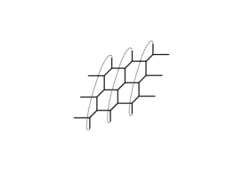
We would upgrade the operation of the geometric transition in the refined topological string theory where the partition function can be in principle evaluated by the refined topological vertex [10, 11] for a given Calabi–Yau geometry (see Appendix A.2 for our convention). As there is a much wide variety of Calabi–Yau geometries, for simplicity and a purpose of the application to qq𝑞𝑞qq-characters, we restrict our argument to a simple class of the geometries visualized by a web diagram in Fig. 1.
Refer to caption
Figure 1: A compactified web diagram which we are considering in the paper.

The thin dotted line connecting the upper and lower end of the diagram represents a compactified direction in the geometry. Note that this type is essentially equipped with the structure of the resolved conifold. It is known that this geometrical data can be dualized to type IIB string theory with D5-branes, NS5-branes, and (1,1)11(1,1)-fivebranes.

One of crucial ingredients in calculating the refined topological string amplitude is the preferred direction on the refined topological vertex. It is an artificial technique for formalism, and final results with different choices of the preferred direction have to coincide (at least without any normalization). However, we claim in this paper that the refined geometric transition should be sensitive to where the preferred direction is set. To explain this point, at first we give a brief review of the prescription for the refined geometric transition that has been used in the literatures [34, 16, 35, 36, 37, 38] in Section 2.1, and then Section 2.2 contains our proposal that actually clarifies the effect of the different selection of the preferred direction. The quantitative argument which we rely on is shown in Section 2.3.

2.1 Conventional prescription

Since there is no established world–sheet description of the refined topological string theory so far, one need to fix a guiding principle for the refined geometric transition from another context. One of frameworks to provide such a principle is the AGT correspondence [17] and its 5d uplift [39, 40]. This duality can be encoded into type IIB string theory presented by the (p,q)𝑝𝑞(p,q)-fivebrane web diagram like Fig. 1. The dictionary between the (p,q)𝑝𝑞(p,q)-web and the geometry allows us to compute the partition function of the corresponding gauge theory by utilizing the refined topological vertex [10, 11], which in the 4d limit turns out to be consistent with the correlation function on the 2d conformal field theory (CFT) side in some cases. Soon after finding the AGT relation, its statement has been extended to include the correspondence between a surface operator in the 4d 𝒩=2𝒩2\mathcal{N}=2 SU(2)2(2) gauge theory and a degenerate field in the Liouville CFT [18]. This circumstance can also be realized in the framework of the (p,q)𝑝𝑞(p,q)-web. The surface operator is engineered by inserting a D3-brane into the (p,q)𝑝𝑞(p,q)-web, which is further mapped to a Lagrangian brane444This is often called a toric brane, however, we do not use this term in the paper since the concerned diagrams here are non-toric. representing a Lagrangian submanifold in the corresponding Calabi–Yau. The computation of the topological string partition function must be incorporated with contributions from open strings when the target space is a Calabi–Yau with specified Lagrangian submanifolds. Although there is no established formula of the refined version of the open topological vertex, this can be evaluated by implementing the geometric transition. In the 4d limit, the result obtained in this way is actually compatible with the correlation function in the presence of a degenerate field in the Liouville CFT.

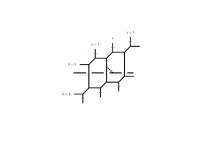
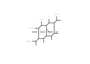
We would sketch concretely the rule of the refined geometric transition that has been lead from the AGT story. On the web diagram as shown in Fig. 1, each internal line implies the topology of 𝐏1superscript𝐏1\mathbb{C}\mathbf{P}^{1} and is equipped with a Kähler modulus. Let Qa(𝔰)superscriptsubscript𝑄𝑎𝔰Q_{a}^{(\mathfrak{s})} be a Kähler modulus for the 𝔰𝔰\mathfrak{s}-th diagonal internal segment from the left in the a𝑎a-th horizontal (uncompactified) line from the top (see Fig. 4 for our convention). The point of calculations along the AGT story with this web diagram is that the preferred direction is chosen on the vertical (compactified) direction, which is depicted as black dots in Fig. 2 (throughout the paper, the vertical axis is always the compactified direction and the horizontal one is uncompactified). The geometric transition can be implemented with the horizontal (uncompactified) line: with appropriately tuning Kähler moduli for diagonal lines attached to the b𝑏b-th horizontal line, this line is detached from the vertical lines and moved away. The geometric transition for the web diagram of our interest is essentially the same as that of the conifold, passing through from the resolved conifold to the deformed conifold and vice versa. If one would like to suspend a Lagrangian brane on the 𝔯𝔯\mathfrak{r}-th vertical line in the process shown in Fig. 2, the Kähler moduli are specialized as555Note that the combination of q1subscript𝑞1q_{1} and q2subscript𝑞2q_{2} depends on ones convention.

Qb(𝔯)superscriptsubscript𝑄𝑏𝔯\displaystyle Q_{b}^{(\mathfrak{r})} =q1mq2nq1q2,absentsuperscriptsubscript𝑞1𝑚superscriptsubscript𝑞2𝑛subscript𝑞1subscript𝑞2\displaystyle=\frac{q_{1}^{m}q_{2}^{n}}{\sqrt{q_{1}q_{2}}}, Qb(𝔰)superscriptsubscript𝑄𝑏𝔰\displaystyle Q_{b}^{(\mathfrak{s})} =1q1q2 for 𝔰𝔯,absent1subscript𝑞1subscript𝑞2 for 𝔰𝔯\displaystyle=\frac{1}{\sqrt{q_{1}q_{2}}}\hskip 5.0pt\text{ for }\mathfrak{s}\neq\mathfrak{r}, (2.1)

with m,n𝑚𝑛m,n\in\mathbb{Z}. This prescription can nicely produce the AGT relation with the surface operator. Consequently, the refined geometric transition associated with the unpreferred direction is operated by (2.1).
Refer to caption \longleftrightarrow Refer to caption
Figure 2: The geometric transition operated on the unpreferred direction. The horizontal axis is compactified and the dots indicate the preferred direction.

We are closing the review with commenting on the integers m,n𝑚𝑛m,n in (2.1). It has been argued in [16] that, in the 4d limit, the adjustment such that m,n>0𝑚𝑛0m,n>0 might produce general (non–elementary) surface operators supported on the surface described by

z1mz2n=0,superscriptsubscript𝑧1𝑚superscriptsubscript𝑧2𝑛0\displaystyle z_{1}^{m}z_{2}^{n}=0, (2.2)

where (z1,z2)subscript𝑧1subscript𝑧2(z_{1},z_{2}) are complex coordinates on two-dimensional planes respecting the rotation by the ΩΩ\Omega-background parameters (ϵ1,ϵ2)subscriptitalic-ϵ1subscriptitalic-ϵ2(\epsilon_{1},\epsilon_{2}), respectively. This discussion seems to work for such physical surface operators, however, for the present we do not have a requirement to restrict the range of m,n𝑚𝑛m,n to be non-negative from the refined topological string point of view. This is why we take m,n𝑚𝑛m,n to run for all integers. Although the refined geometric transition with m,n<0𝑚𝑛0m,n<0 would engineer the unphysical surface operators in the sense that these do not follow the standard discussion (2.2), such branes at least in the unrefined (q1q2=1subscript𝑞1subscript𝑞21q_{1}q_{2}=1) context are referred to as anti-branes [41]. We would return to this point in Section 4.

2.2 New prescription

We turn to giving our new prescription for the refined geometric transition that takes the issues of the preferred direction into account. On computing the refined topological string amplitude for the web diagram of our main interest, the preferred direction is chosen along the horizontal, i.e., uncompactified direction, marked by dots in Fig. 3. The difference of the preferred direction from the previous situation requires us to introduce small modification for the refined geometric transition. In this subsection, we write down the process to implement the refined geometric transition for the current choice of the preferred direction.

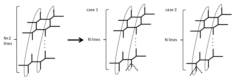
A point which we should stress is to put the preferred direction on the uncompactified (horizontal) direction where the geometric transition can be carried out. In addition, for consistency, it is required that the contributions from the Lagrangian brane is not produced if the web with (M,N)𝑀𝑁(M,N) lines simply reduces to the one with (M,N1)𝑀𝑁1(M,N-1) lines without the Lagrangian brane after the geometric transition, where M𝑀M and N𝑁N stand for the number of compactified (vertical) and uncompactified (horizontal) lines, respectively (see Fig. 4(a)).
Refer to caption \longleftrightarrow Refer to caption
Figure 3: The geometric transition operated on the preferred direction. The horizontal axis is compactified and the dots indicate the preferred direction.

Let us consider the geometric transition that is executed on the b𝑏b-th horizontal line with the Lagrangian brane emerging on the 𝔯𝔯\mathfrak{r}-th vertical line (Fig. 3). Our proposal for the refined geometric transition under the above requirement is comprised of the following three steps:

  1. 0.

    As a supposition the preferred direction is taken to be the uncompactified axis (horizontal here), and then one computes the refined closed topological string amplitude as done in [42, 43].

  2. 1.

    For 𝔰𝔯𝔰𝔯\mathfrak{s}\geq\mathfrak{r}, variables wab(𝔰)(i,j)superscriptsubscript𝑤𝑎𝑏𝔰𝑖𝑗w_{ab}^{(\mathfrak{s})}(i,j) and uab(𝔰)(i,j)superscriptsubscript𝑢𝑎𝑏𝔰𝑖𝑗u_{ab}^{(\mathfrak{s})}(i,j) defined in (2.7), which appear in the generic partition function (2.6), are shifted by using the inversion (A.8) and the difference equation (A.9) of the theta function,

    θ1(e2πiwab(𝔰)(i,j))=Qτ1/2e2πiwab(𝔰)(i,j)×θ1(Qτ1e2πiwab(𝔰)(i,j)),θ1(e2πiuab(𝔰)(i,j))=Qτ1/2e2πiuab(𝔰)(i,j)×θ1(Qτ1e2πiuab(𝔰)(i,j)).subscript𝜃1superscript𝑒2𝜋isuperscriptsubscript𝑤𝑎𝑏𝔰𝑖𝑗absentsuperscriptsubscript𝑄𝜏12superscript𝑒2𝜋isuperscriptsubscript𝑤𝑎𝑏𝔰𝑖𝑗subscript𝜃1superscriptsubscript𝑄𝜏1superscript𝑒2𝜋isuperscriptsubscript𝑤𝑎𝑏𝔰𝑖𝑗subscript𝜃1superscript𝑒2𝜋isuperscriptsubscript𝑢𝑎𝑏𝔰𝑖𝑗absentsuperscriptsubscript𝑄𝜏12superscript𝑒2𝜋isuperscriptsubscript𝑢𝑎𝑏𝔰𝑖𝑗subscript𝜃1superscriptsubscript𝑄𝜏1superscript𝑒2𝜋isuperscriptsubscript𝑢𝑎𝑏𝔰𝑖𝑗\displaystyle\begin{aligned} \theta_{1}\left(e^{2\pi\mathrm{i}w_{ab}^{(\mathfrak{s})}(i,j)}\right)&=Q_{\tau}^{1/2}e^{2\pi\mathrm{i}w_{ab}^{(\mathfrak{s})}(i,j)}\times\theta_{1}\left(Q_{\tau}^{-1}e^{-2\pi\mathrm{i}w_{ab}^{(\mathfrak{s})}(i,j)}\right),\\ \theta_{1}\left(e^{2\pi\mathrm{i}u_{ab}^{(\mathfrak{s})}(i,j)}\right)&=Q_{\tau}^{1/2}e^{2\pi\mathrm{i}u_{ab}^{(\mathfrak{s})}(i,j)}\times\theta_{1}\left(Q_{\tau}^{-1}e^{-2\pi\mathrm{i}u_{ab}^{(\mathfrak{s})}(i,j)}\right).\end{aligned} (2.3)
  3. 2.

    Then, tuning the Kähler moduli as

    Qb(𝔰)superscriptsubscript𝑄𝑏𝔰\displaystyle Q_{b}^{(\mathfrak{s})} =1q1q2(𝔰<𝔯),absent1subscript𝑞1subscript𝑞2𝔰𝔯\displaystyle=\frac{1}{\sqrt{q_{1}q_{2}}}\hskip 15.00002pt(\mathfrak{s}<\mathfrak{r}), Qb(𝔯)superscriptsubscript𝑄𝑏𝔯\displaystyle Q_{b}^{(\mathfrak{r})} =q1mq2nq1q2,absentsuperscriptsubscript𝑞1𝑚superscriptsubscript𝑞2𝑛subscript𝑞1subscript𝑞2\displaystyle=\frac{q_{1}^{m}q_{2}^{n}}{\sqrt{q_{1}q_{2}}}, Qb(𝔰)superscriptsubscript𝑄𝑏𝔰\displaystyle Q_{b}^{(\mathfrak{s})} =q1q2(𝔰>𝔯),absentsubscript𝑞1subscript𝑞2𝔰𝔯\displaystyle=\sqrt{q_{1}q_{2}}\hskip 15.00002pt(\mathfrak{s}>\mathfrak{r}), (2.4)

    with m,n𝑚𝑛m,n\in\mathbb{Z}.

  4. 3.

    Finally, shifting variables wab(𝔯)(i,j)superscriptsubscript𝑤𝑎𝑏𝔯𝑖𝑗w_{ab}^{(\mathfrak{r})}(i,j) for all a𝑎a by hand,

    wab(𝔯)(i,j)wab(𝔯)(i,j)ϵ1ϵ2,superscriptsubscript𝑤𝑎𝑏𝔯𝑖𝑗superscriptsubscript𝑤𝑎𝑏𝔯𝑖𝑗subscriptitalic-ϵ1subscriptitalic-ϵ2\displaystyle w_{ab}^{(\mathfrak{r})}(i,j)\to w_{ab}^{(\mathfrak{r})}(i,j)-\epsilon_{1}-\epsilon_{2}, (2.5)

    while others in (2.7) are kept unchanged.

We should make a comment on the shift of step 3 in our prescription. The shift (2.5) has nothing to do with the Kähler parameters: any Kähler parameter is not shifted together with this operation, but rather, with viewing wab(𝔯)(i,j)superscriptsubscript𝑤𝑎𝑏𝔯𝑖𝑗w_{ab}^{(\mathfrak{r})}(i,j) as a single variable, it is just to add ϵ1ϵ2subscriptitalic-ϵ1subscriptitalic-ϵ2-\epsilon_{1}-\epsilon_{2} to it. This is purely a technical thing which is originated from the difference of the specialization (2.4) of the Kähler moduli Qb(𝔰)superscriptsubscript𝑄𝑏𝔰Q_{b}^{(\mathfrak{s})} for 𝔰<𝔯𝔰𝔯\mathfrak{s}<\mathfrak{r} and 𝔰>𝔯𝔰𝔯\mathfrak{s}>\mathfrak{r}. The reason why we need this shift is to satisfy the requirement for consistency that the refined geometric transition without generating a Lagrangian brane reproduces the closed topological string amplitude (see below for numerical details). The step 2 and 3 reflect the dependence of the refined geometric transition on the preferred direction. Indeed, it is expected that, even though the closed topological string amplitude should be independent of the preferred direction, the open one really depends on whether or not the Lagrangian brane is attached to the preferred direction (see, e.g., [44, 45]). This is basically because the Lagrangian brane can end on the (p,q)𝑝𝑞(p,q)-fivebrane with general (p,q)𝑝𝑞(p,q), therefore the geometric transition should be characterized by (p,q)𝑝𝑞(p,q) in addition to (m,n)𝑚𝑛(m,n). This implies that the position of the preferred direction put on the (p,q)𝑝𝑞(p,q)-fivebrane leads to the inequivalent result of the open topological string amplitude. Both procedures of the refined geometric transition can reproduce correctly the identical result in the unrefined limit q1q2=1subscript𝑞1subscript𝑞21q_{1}q_{2}=1 as expected. Our prescription seems compatible with this suggestion.

A Lagrangian brane appears on only one vertical line upon a single sequence of the above geometric transition. If one desires to generate several Lagrangian branes on different vertical lines for a web diagram, it is necessary to consider a bigger web and repeat the procedure (2.3)-(2.5) many times (as demonstrated in Section 3).

We will devote the next subsection to showing quantitative clarification how this process works and produces the refined topological string amplitude incorporating the contribution of the Lagrangian brane. In Section 3, it will be discussed that the refined geometric transition initiated by our prescription gives possibly how to realize the qq𝑞𝑞qq-character from string theory.

2.3 Derivation

Our prescription given above seems a bit intricate rather than (2.1), and we would explain here why this works when the uncompactified line assigned with the preferred direction is removed upon the geometric transition.

2.3.1 General formula for the partition function

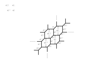
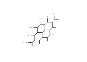
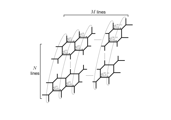
We are now concentrating on the compactified web shown as Fig. 4 with general (M,N)𝑀𝑁(M,N) lines. On the technique of the refined topological vertex (A.2), the partition function 𝒵M,Nsubscript𝒵𝑀𝑁\mathcal{Z}_{M,N} for this web diagram has been derived as [43]
Refer to caption (a) Entire web                Refer to caption (b) Internal hexagons
Figure 4: The web diagram with M𝑀M vertical and N𝑁N horizontal lines.
𝒵M,N={μa(𝔰)}a=1,,N𝔰=1,,M1𝔰=1M1a=1N(Q¯f,a(𝔰))|μa(𝔰)|(i,j)μa(𝔰)b=1Nθ1(e2πizab(𝔰)(i,j))θ1(e2πiwab(𝔰)(i,j))θ1(e2πiuab(𝔰)(i,j))θ1(e2πivab(𝔰)(i,j)),subscript𝒵𝑀𝑁subscriptsuperscriptsubscriptsuperscriptsubscript𝜇𝑎𝔰𝑎1𝑁𝔰1𝑀1superscriptsubscriptproduct𝔰1𝑀1superscriptsubscriptproduct𝑎1𝑁superscriptsuperscriptsubscript¯𝑄𝑓𝑎𝔰subscriptsuperscript𝜇𝔰𝑎subscriptproduct𝑖𝑗subscriptsuperscript𝜇𝔰𝑎superscriptsubscriptproduct𝑏1𝑁subscript𝜃1superscript𝑒2𝜋isuperscriptsubscript𝑧𝑎𝑏𝔰𝑖𝑗subscript𝜃1superscript𝑒2𝜋isuperscriptsubscript𝑤𝑎𝑏𝔰𝑖𝑗subscript𝜃1superscript𝑒2𝜋isuperscriptsubscript𝑢𝑎𝑏𝔰𝑖𝑗subscript𝜃1superscript𝑒2𝜋isuperscriptsubscript𝑣𝑎𝑏𝔰𝑖𝑗\displaystyle\mathcal{Z}_{M,N}=\sum_{\{\mu_{a}^{(\mathfrak{s})}\}_{a=1,\cdots,N}^{\mathfrak{s}=1,\cdots,M-1}}\prod_{\mathfrak{s}=1}^{M-1}\prod_{a=1}^{N}\left(\bar{Q}_{f,a}^{(\mathfrak{s})}\right)^{|\mu^{(\mathfrak{s})}_{a}|}\prod_{(i,j)\in\mu^{(\mathfrak{s})}_{a}}\prod_{b=1}^{N}{\theta_{1}(e^{2\pi\mathrm{i}z_{ab}^{(\mathfrak{s})}(i,j)})\theta_{1}(e^{2\pi\mathrm{i}w_{ab}^{(\mathfrak{s})}(i,j)})\over\theta_{1}(e^{2\pi\mathrm{i}u_{ab}^{(\mathfrak{s})}(i,j)})\theta_{1}(e^{2\pi\mathrm{i}v_{ab}^{(\mathfrak{s})}(i,j)})}, (2.6)

where

e2πizab(𝔰)(i,j)=(Qab(𝔰+1))1q1μb,j(𝔰+1),t+i1/2q2μa,i(𝔰)j+1/2,e2πiwab(𝔰)(i,j)=(Qba(𝔰))1q1μb,j(𝔰1),ti+1/2q2μa,i(𝔰)+j1/2,e2πiuab(𝔰)(i,j)=(Q^ba(𝔰))1q1μb,j(𝔰),ti+1q2μa,i(𝔰)+j,e2πivab(𝔰)(i,j)=(Q^ab(𝔰))1q1μb,j(𝔰),t+iq2μa,i(𝔰)j+1,superscript𝑒2𝜋isuperscriptsubscript𝑧𝑎𝑏𝔰𝑖𝑗absentsuperscriptsuperscriptsubscript𝑄𝑎𝑏𝔰11superscriptsubscript𝑞1superscriptsubscript𝜇𝑏𝑗𝔰1𝑡𝑖12superscriptsubscript𝑞2superscriptsubscript𝜇𝑎𝑖𝔰𝑗12superscript𝑒2𝜋isuperscriptsubscript𝑤𝑎𝑏𝔰𝑖𝑗absentsuperscriptsuperscriptsubscript𝑄𝑏𝑎𝔰1superscriptsubscript𝑞1superscriptsubscript𝜇𝑏𝑗𝔰1𝑡𝑖12superscriptsubscript𝑞2superscriptsubscript𝜇𝑎𝑖𝔰𝑗12superscript𝑒2𝜋isuperscriptsubscript𝑢𝑎𝑏𝔰𝑖𝑗absentsuperscriptsuperscriptsubscript^𝑄𝑏𝑎𝔰1superscriptsubscript𝑞1superscriptsubscript𝜇𝑏𝑗𝔰𝑡𝑖1superscriptsubscript𝑞2superscriptsubscript𝜇𝑎𝑖𝔰𝑗superscript𝑒2𝜋isuperscriptsubscript𝑣𝑎𝑏𝔰𝑖𝑗absentsuperscriptsuperscriptsubscript^𝑄𝑎𝑏𝔰1superscriptsubscript𝑞1superscriptsubscript𝜇𝑏𝑗𝔰𝑡𝑖superscriptsubscript𝑞2superscriptsubscript𝜇𝑎𝑖𝔰𝑗1\displaystyle\begin{aligned} e^{2\pi\mathrm{i}z_{ab}^{(\mathfrak{s})}(i,j)}&=\left(Q_{ab}^{(\mathfrak{s}+1)}\right)^{-1}q_{1}^{-\mu_{b,j}^{(\mathfrak{s}+1),t}+i-1/2}q_{2}^{\mu_{a,i}^{(\mathfrak{s})}-j+1/2},\\ e^{2\pi\mathrm{i}w_{ab}^{(\mathfrak{s})}(i,j)}&=\left(Q_{ba}^{(\mathfrak{s})}\right)^{-1}q_{1}^{\mu_{b,j}^{(\mathfrak{s}-1),t}-i+1/2}q_{2}^{-\mu_{a,i}^{(\mathfrak{s})}+j-1/2},\\ e^{2\pi\mathrm{i}u_{ab}^{(\mathfrak{s})}(i,j)}&=\left(\hat{Q}_{ba}^{(\mathfrak{s})}\right)^{-1}q_{1}^{\mu_{b,j}^{(\mathfrak{s}),t}-i+1}q_{2}^{-\mu_{a,i}^{(\mathfrak{s})}+j},\\ e^{2\pi\mathrm{i}v_{ab}^{(\mathfrak{s})}(i,j)}&=\left(\hat{Q}_{ab}^{(\mathfrak{s})}\right)^{-1}q_{1}^{-\mu_{b,j}^{(\mathfrak{s}),t}+i}q_{2}^{\mu_{a,i}^{(\mathfrak{s})}-j+1},\end{aligned} (2.7)

with t𝑡t representing the transpose of the Young diagram (Fig. 11(c)). We collect the definitions and notations in Appendix A. Note that, for simplicity, we omit a complex parameter Qτ:=e2πiτassignsubscript𝑄𝜏superscript𝑒2𝜋i𝜏Q_{\tau}:=e^{2\pi\mathrm{i}\tau} in the theta function as θ1(x)subscript𝜃1𝑥\theta_{1}(x) unless otherwise stated. We denote the Kähler moduli for diagonal, vertical, and horizontal internal segments by Qa(𝔰)superscriptsubscript𝑄𝑎𝔰Q_{a}^{(\mathfrak{s})}, Q~a(𝔰)superscriptsubscript~𝑄𝑎𝔰\tilde{Q}_{a}^{(\mathfrak{s})}, and Qf,a(𝔰)superscriptsubscript𝑄𝑓𝑎𝔰Q_{f,a}^{(\mathfrak{s})}, respectively, which are visualized in Fig. 4(a) and 4(b). The weights in the partition function, corresponding to instanton counting parameters in the Nekrasov partition function, are given by

Q¯f,a(𝔰)=(q1q2)N12Qf,a(𝔰)b=1NQb(𝔰).superscriptsubscript¯𝑄𝑓𝑎𝔰superscriptsubscript𝑞1subscript𝑞2𝑁12superscriptsubscript𝑄𝑓𝑎𝔰superscriptsubscriptproduct𝑏1𝑁superscriptsubscript𝑄𝑏𝔰\displaystyle\bar{Q}_{f,a}^{(\mathfrak{s})}=\left(q_{1}q_{2}\right)^{N-1\over 2}Q_{f,a}^{(\mathfrak{s})}\prod_{b=1}^{N}Q_{b}^{(\mathfrak{s})}. (2.8)

Also, we use the simplified symbols for the products of the Kähler moduli in the variables (2.7), defined as

Qab(𝔰)superscriptsubscript𝑄𝑎𝑏𝔰\displaystyle Q_{ab}^{(\mathfrak{s})} ={Qa(𝔰)i=bNQτi(𝔰)(mod Qτ)for a=1,Qa(𝔰)i=1a1Qτi(𝔰)j=bNQτj(𝔰)(mod Qτ)for a1,\displaystyle=\left\{\begin{aligned} &Q_{a}^{(\mathfrak{s})}\prod_{i=b}^{N}Q_{\tau_{i}}^{(\mathfrak{s})}&&(\text{mod }Q_{\tau})&&\text{for }a=1,\\ &Q_{a}^{(\mathfrak{s})}\prod_{i=1}^{a-1}Q_{\tau_{i}}^{(\mathfrak{s})}\prod_{j=b}^{N}Q_{\tau_{j}}^{(\mathfrak{s})}&&(\text{mod }Q_{\tau})&&\text{for }a\neq 1,\end{aligned}\right. (2.9)

for the numerator, and

Q^ab(𝔰)superscriptsubscript^𝑄𝑎𝑏𝔰\displaystyle\hat{Q}_{ab}^{(\mathfrak{s})} ={i=ba1Qτi(𝔰)for a>b,1for a=b,Qτ/i=ab1Qτi(𝔰)for a<b,\displaystyle=\left\{\begin{aligned} &\prod_{i=b}^{a-1}Q_{\tau_{i}}^{(\mathfrak{s})}&&\text{for }a>b,\\ &1&&\text{for }a=b,\\ &Q_{\tau}\left/\prod_{i=a}^{b-1}Q^{(\mathfrak{s})}_{\tau_{i}}\right.&&\text{for }a<b,\end{aligned}\right. (2.10)

for the denominator, where

Qτi(𝔰):=Qi(𝔰)Q~i(𝔰)=Q~i(𝔰+1)Qi+1(𝔰+1).assignsubscriptsuperscript𝑄𝔰subscript𝜏𝑖superscriptsubscript𝑄𝑖𝔰superscriptsubscript~𝑄𝑖𝔰superscriptsubscript~𝑄𝑖𝔰1superscriptsubscript𝑄𝑖1𝔰1\displaystyle Q^{(\mathfrak{s})}_{\tau_{i}}:=Q_{i}^{(\mathfrak{s})}\tilde{Q}_{i}^{(\mathfrak{s})}=\tilde{Q}_{i}^{(\mathfrak{s}+1)}Q_{i+1}^{(\mathfrak{s}+1)}. (2.11)

The second equality follows from the consistency condition to form internal hexagons (Fig. 4(b)). It has been revealed that this geometry actually realizes an elliptically fibered Calabi–Yau with the complex modulus Qτsubscript𝑄𝜏Q_{\tau} identified as

Qτ=a=1NQτa(𝔰)for 𝔰.subscript𝑄𝜏superscriptsubscriptproduct𝑎1𝑁superscriptsubscript𝑄subscript𝜏𝑎𝔰for for-all𝔰\displaystyle Q_{\tau}=\prod_{a=1}^{N}Q_{\tau_{a}}^{(\mathfrak{s})}\hskip 20.00003pt\text{for }\forall\mathfrak{s}. (2.12)

We comment on the M-theory uplift of this picture. It is well known that type IIB string theory compactified on S1superscript𝑆1S^{1} is dual to M-theory on the torus T2superscript𝑇2T^{2}. The web as in Fig. 4 is rendered to the M-theory brane configuration where the stacks of M2-branes are suspended between separated M𝑀M M5-branes on an asymptotically locally Euclidean (ALE) space equipped with Nsubscript𝑁\mathbb{Z}_{N} orbifolding. This duality supports the fact that the low energy theory on the present (p,q)𝑝𝑞(p,q)-web are described by the tensor branch of the corresponding 6d 𝒩=(1,0)𝒩10\mathcal{N}=(1,0) theory. It has been argued in [42, 43] that the partition function (2.6) captures the spectra of self-dual strings, called M-strings, wrapping T2superscript𝑇2T^{2} in the 6d theory, and the Young diagrams μa(𝔰)superscriptsubscript𝜇𝑎𝔰\mu_{a}^{(\mathfrak{s})} label the ground states of M-strings.

2.3.2 Actual process of the geometric transition

When we perform the geometric transition on the b𝑏b-th horizontal line such that the Lagrangian brane appears on the 𝔯𝔯\mathfrak{r}-th vertical line, the main contribution that should be carefully treated is

(i,j)μa(𝔰)θ1(e2πizab(𝔰)(i,j))θ1(e2πiwab(𝔰)(i,j))θ1(e2πiuab(𝔰)(i,j))θ1(e2πivab(𝔰)(i,j))subscriptproduct𝑖𝑗superscriptsubscript𝜇𝑎𝔰subscript𝜃1superscript𝑒2𝜋isuperscriptsubscript𝑧𝑎𝑏𝔰𝑖𝑗subscript𝜃1superscript𝑒2𝜋isuperscriptsubscript𝑤𝑎𝑏𝔰𝑖𝑗subscript𝜃1superscript𝑒2𝜋isuperscriptsubscript𝑢𝑎𝑏𝔰𝑖𝑗subscript𝜃1superscript𝑒2𝜋isuperscriptsubscript𝑣𝑎𝑏𝔰𝑖𝑗\displaystyle\prod_{(i,j)\in\mu_{a}^{(\mathfrak{s})}}{\theta_{1}\left(e^{2\pi\mathrm{i}z_{ab}^{(\mathfrak{s})}(i,j)}\right)\theta_{1}\left(e^{2\pi\mathrm{i}w_{ab}^{(\mathfrak{s})}(i,j)}\right)\over\theta_{1}\left(e^{2\pi\mathrm{i}u_{ab}^{(\mathfrak{s})}(i,j)}\right)\theta_{1}\left(e^{2\pi\mathrm{i}v_{ab}^{(\mathfrak{s})}(i,j)}\right)} (2.13)

for all a𝑎a. We would divide the calculation process for this into two parts with 𝔰<𝔯𝔰𝔯\mathfrak{s}<\mathfrak{r} and 𝔰𝔯𝔰𝔯\mathfrak{s}\geq\mathfrak{r}. Remark that we sometimes implicitly use the relation (2.12) to change the variables.

For 𝔰<𝔯𝔰𝔯\mathfrak{s}<\mathfrak{r}

We firstly focus on the sector for 𝔰<𝔯𝔰𝔯\mathfrak{s}<\mathfrak{r} where the geometric transition (2.4) can straightforwardly work. One can easily see that (2.13) does not produce the nontrivial contribution unless

μb(𝔰)= for 𝔰.superscriptsubscript𝜇𝑏𝔰 for for-all𝔰\displaystyle\mu_{b}^{(\mathfrak{s})}=\emptyset\text{ for }\forall\mathfrak{s}. (2.14)

Accordingly, this condition is necessary in order to obtain the appropriate result for the partition function obtained via the geometric transition. Then, variables zab(𝔰)(i,j)superscriptsubscript𝑧𝑎𝑏𝔰𝑖𝑗z_{ab}^{(\mathfrak{s})}(i,j) and wab(𝔰)(i,j)superscriptsubscript𝑤𝑎𝑏𝔰𝑖𝑗w_{ab}^{(\mathfrak{s})}(i,j) can be rewritten as

θ1(e2πizab(𝔰)(i,j))subscript𝜃1superscript𝑒2𝜋isuperscriptsubscript𝑧𝑎𝑏𝔰𝑖𝑗\displaystyle\theta_{1}\left(e^{2\pi\mathrm{i}z_{ab}^{(\mathfrak{s})}(i,j)}\right) =θ1((q1q2Qb(𝔰+1))1e2πivab(𝔰)(i,j)),absentsubscript𝜃1superscriptsubscript𝑞1subscript𝑞2superscriptsubscript𝑄𝑏𝔰11superscript𝑒2𝜋isuperscriptsubscript𝑣𝑎𝑏𝔰𝑖𝑗\displaystyle=\theta_{1}\left(\left(\sqrt{q_{1}q_{2}}Q_{b}^{(\mathfrak{s}+1)}\right)^{-1}e^{2\pi\mathrm{i}v_{ab}^{(\mathfrak{s})}(i,j)}\right), (2.15)
θ1(e2πiwab(𝔰)(i,j))subscript𝜃1superscript𝑒2𝜋isuperscriptsubscript𝑤𝑎𝑏𝔰𝑖𝑗\displaystyle\theta_{1}\left(e^{2\pi\mathrm{i}w_{ab}^{(\mathfrak{s})}(i,j)}\right) =θ1((q1q2Qb(𝔰))1e2πiuab(𝔰)(i,j)),absentsubscript𝜃1superscriptsubscript𝑞1subscript𝑞2superscriptsubscript𝑄𝑏𝔰1superscript𝑒2𝜋isuperscriptsubscript𝑢𝑎𝑏𝔰𝑖𝑗\displaystyle=\theta_{1}\left(\left(\sqrt{q_{1}q_{2}}Q_{b}^{(\mathfrak{s})}\right)^{-1}e^{2\pi\mathrm{i}u_{ab}^{(\mathfrak{s})}(i,j)}\right), (2.16)

where we used the relation (2.11) for zab(𝔰)(i,j)superscriptsubscript𝑧𝑎𝑏𝔰𝑖𝑗z_{ab}^{(\mathfrak{s})}(i,j). With these expressions, the specialization (2.4) of the Kähler moduli results in

(2.13)1for 𝔰<𝔯1,formulae-sequenceitalic-(2.13italic-)1for 𝔰𝔯1\displaystyle\eqref{deri5}\to 1\hskip 20.00003pt\text{for }\mathfrak{s}<\mathfrak{r}-1, (2.17)

and

(2.13)(i,j)μa(𝔯1)θ1(q1mq2ne2πivab(𝔯1)(i,j))θ1(e2πivab(𝔯1)(i,j))for 𝔰=𝔯1.formulae-sequenceitalic-(2.13italic-)subscriptproduct𝑖𝑗superscriptsubscript𝜇𝑎𝔯1subscript𝜃1superscriptsubscript𝑞1𝑚superscriptsubscript𝑞2𝑛superscript𝑒2𝜋isuperscriptsubscript𝑣𝑎𝑏𝔯1𝑖𝑗subscript𝜃1superscript𝑒2𝜋isuperscriptsubscript𝑣𝑎𝑏𝔯1𝑖𝑗for 𝔰𝔯1\displaystyle\eqref{deri5}\to\prod_{(i,j)\in\mu_{a}^{(\mathfrak{r}-1)}}{\theta_{1}\left(q_{1}^{m}q_{2}^{n}e^{2\pi\mathrm{i}v_{ab}^{(\mathfrak{r}-1)}(i,j)}\right)\over\theta_{1}\left(e^{2\pi\mathrm{i}v_{ab}^{(\mathfrak{r}-1)}(i,j)}\right)}\hskip 20.00003pt\text{for }\mathfrak{s}=\mathfrak{r}-1. (2.18)

Indeed, (2.18) is the half of the contributions of the Lagrangian brane. This is just what we want because this reduces to 111 when m=n=0𝑚𝑛0m=n=0, namely, no Lagrangian brane appear, as required. Actually, this expression matches with the result of [46]. Moreover, the weights in the sum of the Young diagrams change as

Q¯f,a(𝔰)(q1q2)(N1)12Qf,a(𝔰) =c1 cb NQc(𝔰),superscriptsubscript¯𝑄𝑓𝑎𝔰superscriptsubscript𝑞1subscript𝑞2𝑁112superscriptsubscript𝑄𝑓𝑎𝔰superscriptsubscriptproduct =c1 cb 𝑁superscriptsubscript𝑄𝑐𝔰\displaystyle\bar{Q}_{f,a}^{(\mathfrak{s})}\to\left(q_{1}q_{2}\right)^{(N-1)-1\over 2}Q_{f,a}^{(\mathfrak{s})}\prod_{\shortstack{${\scriptstyle c=1}$ \\ ${\scriptstyle c\neq b}$ }}^{N}Q_{c}^{(\mathfrak{s})}, (2.19)

and this is nothing but the ones in the partition function for the web diagram with (M,N1)𝑀𝑁1(M,N-1) lines. Our prescription for the refined geometric transition appropriately works for 𝔰<𝔯𝔰𝔯\mathfrak{s}<\mathfrak{r}.

For 𝔰𝔯𝔰𝔯\mathfrak{s}\geq\mathfrak{r}

Let us turn to the sector for 𝔰𝔯𝔰𝔯\mathfrak{s}\geq\mathfrak{r}. In addition to the first step (2.3), by using (2.11), the relation

θ1(e2πizab(𝔰)(i,j))subscript𝜃1superscript𝑒2𝜋isuperscriptsubscript𝑧𝑎𝑏𝔰𝑖𝑗\displaystyle\theta_{1}\left(e^{2\pi\mathrm{i}z_{ab}^{(\mathfrak{s})}(i,j)}\right) =θ1((Qb(𝔰+1)Qτq1q2)1e2πiuab(𝔰)(i,j))absentsubscript𝜃1superscriptsuperscriptsubscript𝑄𝑏𝔰1subscript𝑄𝜏subscript𝑞1subscript𝑞21superscript𝑒2𝜋isuperscriptsubscript𝑢𝑎𝑏𝔰𝑖𝑗\displaystyle=\theta_{1}\left(\left(\frac{Q_{b}^{(\mathfrak{s}+1)}Q_{\tau}}{\sqrt{q_{1}q_{2}}}\right)^{-1}e^{-2\pi\mathrm{i}u_{ab}^{(\mathfrak{s})}(i,j)}\right) (2.20)

holds under the restriction (2.14). As a result, we have

(2.13)italic-(2.13italic-)\displaystyle\eqref{deri5} (i,j)μa(𝔰)e2πi(wab(𝔰)(i,j)uab(𝔰)(i,j))θ1((Qb(𝔰+1)q1q2)1Qτ1e2πiuab(𝔰)(i,j))θ1(Qτ1e2πiwab(𝔰)(i,j))θ1(Qτ1e2πiuab(𝔰)(i,j))θ1(e2πivab(𝔰)(i,j))absentsubscriptproduct𝑖𝑗superscriptsubscript𝜇𝑎𝔰superscript𝑒2𝜋isuperscriptsubscript𝑤𝑎𝑏𝔰𝑖𝑗superscriptsubscript𝑢𝑎𝑏𝔰𝑖𝑗subscript𝜃1superscriptsuperscriptsubscript𝑄𝑏𝔰1subscript𝑞1subscript𝑞21superscriptsubscript𝑄𝜏1superscript𝑒2𝜋isuperscriptsubscript𝑢𝑎𝑏𝔰𝑖𝑗subscript𝜃1superscriptsubscript𝑄𝜏1superscript𝑒2𝜋isuperscriptsubscript𝑤𝑎𝑏𝔰𝑖𝑗subscript𝜃1superscriptsubscript𝑄𝜏1superscript𝑒2𝜋isuperscriptsubscript𝑢𝑎𝑏𝔰𝑖𝑗subscript𝜃1superscript𝑒2𝜋isuperscriptsubscript𝑣𝑎𝑏𝔰𝑖𝑗\displaystyle\to\prod_{(i,j)\in\mu_{a}^{(\mathfrak{s})}}e^{2\pi\mathrm{i}(w_{ab}^{(\mathfrak{s})}(i,j)-u_{ab}^{(\mathfrak{s})}(i,j))}{\theta_{1}\left(\left(\frac{Q_{b}^{(\mathfrak{s}+1)}}{\sqrt{q_{1}q_{2}}}\right)^{-1}Q_{\tau}^{-1}e^{-2\pi\mathrm{i}u_{ab}^{(\mathfrak{s})}(i,j)}\right)\theta_{1}\left(Q_{\tau}^{-1}e^{-2\pi\mathrm{i}w_{ab}^{(\mathfrak{s})}(i,j)}\right)\over\theta_{1}\left(Q_{\tau}^{-1}e^{-2\pi\mathrm{i}u_{ab}^{(\mathfrak{s})}(i,j)}\right)\theta_{1}\left(e^{2\pi\mathrm{i}v_{ab}^{(\mathfrak{s})}(i,j)}\right)}
=(q1q2Qb(𝔰))|μa(𝔰)|(i,j)μa(𝔰)θ1((Qb(𝔰+1)q1q2)1Qτ1e2πiuab(𝔰)(i,j))θ1(Qτ1e2πiwab(𝔰)(i,j))θ1(Qτ1e2πiuab(𝔰)(i,j))θ1(e2πivab(𝔰)(i,j)),absentsuperscriptsubscript𝑞1subscript𝑞2superscriptsubscript𝑄𝑏𝔰superscriptsubscript𝜇𝑎𝔰subscriptproduct𝑖𝑗superscriptsubscript𝜇𝑎𝔰subscript𝜃1superscriptsuperscriptsubscript𝑄𝑏𝔰1subscript𝑞1subscript𝑞21superscriptsubscript𝑄𝜏1superscript𝑒2𝜋isuperscriptsubscript𝑢𝑎𝑏𝔰𝑖𝑗subscript𝜃1superscriptsubscript𝑄𝜏1superscript𝑒2𝜋isuperscriptsubscript𝑤𝑎𝑏𝔰𝑖𝑗subscript𝜃1superscriptsubscript𝑄𝜏1superscript𝑒2𝜋isuperscriptsubscript𝑢𝑎𝑏𝔰𝑖𝑗subscript𝜃1superscript𝑒2𝜋isuperscriptsubscript𝑣𝑎𝑏𝔰𝑖𝑗\displaystyle=\left(\sqrt{q_{1}q_{2}}Q_{b}^{(\mathfrak{s})}\right)^{-|\mu_{a}^{(\mathfrak{s})}|}\prod_{(i,j)\in\mu_{a}^{(\mathfrak{s})}}{\theta_{1}\left(\left(\frac{Q_{b}^{(\mathfrak{s}+1)}}{\sqrt{q_{1}q_{2}}}\right)^{-1}Q_{\tau}^{-1}e^{-2\pi\mathrm{i}u_{ab}^{(\mathfrak{s})}(i,j)}\right)\theta_{1}\left(Q_{\tau}^{-1}e^{-2\pi\mathrm{i}w_{ab}^{(\mathfrak{s})}(i,j)}\right)\over\theta_{1}\left(Q_{\tau}^{-1}e^{-2\pi\mathrm{i}u_{ab}^{(\mathfrak{s})}(i,j)}\right)\theta_{1}\left(e^{2\pi\mathrm{i}v_{ab}^{(\mathfrak{s})}(i,j)}\right)}, (2.21)

Similarly for (2.19), the overall factor can be absorbed into the associated weight so that

Q¯f,a(𝔰)(q1q2Qb(𝔰))1=(q1q2)(N1)12Qf,a(𝔰) =c1 cb NQc(𝔰),superscriptsubscript¯𝑄𝑓𝑎𝔰superscriptsubscript𝑞1subscript𝑞2superscriptsubscript𝑄𝑏𝔰1superscriptsubscript𝑞1subscript𝑞2𝑁112superscriptsubscript𝑄𝑓𝑎𝔰superscriptsubscriptproduct =c1 cb 𝑁superscriptsubscript𝑄𝑐𝔰\displaystyle\bar{Q}_{f,a}^{(\mathfrak{s})}\left(\sqrt{q_{1}q_{2}}Q_{b}^{(\mathfrak{s})}\right)^{-1}=\left(q_{1}q_{2}\right)^{(N-1)-1\over 2}Q_{f,a}^{(\mathfrak{s})}\prod_{\shortstack{${\scriptstyle c=1}$ \\ ${\scriptstyle c\neq b}$ }}^{N}Q_{c}^{(\mathfrak{s})}, (2.22)

which becomes the one for the web diagram with (M,N1)𝑀𝑁1(M,N-1) lines. This is the actual reason why our prescription needs the first step (2.3). Then, the parameter tuning (2.4) as the second step leads to

(2.21)1for 𝔰>𝔯,formulae-sequenceitalic-(2.21italic-)1for 𝔰𝔯\displaystyle\eqref{deri1}\to 1\hskip 20.00003pt\text{for }\mathfrak{s}>\mathfrak{r}, (2.23)

and

(2.21)italic-(2.21italic-)\displaystyle\eqref{deri1} (i,j)μa(𝔯)θ1(Qτ1e2πi(wab(𝔯)(i,j)ϵ1ϵ2))θ1(e2πivab(𝔯)(i,j))absentsubscriptproduct𝑖𝑗superscriptsubscript𝜇𝑎𝔯subscript𝜃1superscriptsubscript𝑄𝜏1superscript𝑒2𝜋isuperscriptsubscript𝑤𝑎𝑏𝔯𝑖𝑗subscriptitalic-ϵ1subscriptitalic-ϵ2subscript𝜃1superscript𝑒2𝜋isuperscriptsubscript𝑣𝑎𝑏𝔯𝑖𝑗\displaystyle\to\prod_{(i,j)\in\mu_{a}^{(\mathfrak{r})}}{\theta_{1}\left(Q_{\tau}^{-1}e^{-2\pi\mathrm{i}(w_{ab}^{(\mathfrak{r})}(i,j)-\epsilon_{1}-\epsilon_{2})}\right)\over\theta_{1}\left(e^{2\pi\mathrm{i}v_{ab}^{(\mathfrak{r})}(i,j)}\right)}
=(i,j)μa(𝔯)θ1(Qτ1Qba(𝔯)q1i+1/2q2μa,i(𝔯)j+3/2)θ1(Qτ1Qba(𝔯)q1i+1/2+mq2μa,i(𝔯)j+3/2+n)for 𝔰=𝔯,formulae-sequenceabsentsubscriptproduct𝑖𝑗superscriptsubscript𝜇𝑎𝔯subscript𝜃1superscriptsubscript𝑄𝜏1superscriptsubscript𝑄𝑏𝑎𝔯superscriptsubscript𝑞1𝑖12superscriptsubscript𝑞2superscriptsubscript𝜇𝑎𝑖𝔯𝑗32subscript𝜃1superscriptsubscript𝑄𝜏1superscriptsubscript𝑄𝑏𝑎𝔯superscriptsubscript𝑞1𝑖12𝑚superscriptsubscript𝑞2superscriptsubscript𝜇𝑎𝑖𝔯𝑗32𝑛for 𝔰𝔯\displaystyle=\prod_{(i,j)\in\mu_{a}^{(\mathfrak{r})}}{\theta_{1}\left(Q_{\tau}^{-1}Q_{ba}^{(\mathfrak{r})}q_{1}^{i+1/2}q_{2}^{\mu_{a,i}^{(\mathfrak{r})}-j+3/2}\right)\over\theta_{1}\left(Q_{\tau}^{-1}Q_{ba}^{(\mathfrak{r})}q_{1}^{i+1/2+m}q_{2}^{\mu_{a,i}^{(\mathfrak{r})}-j+3/2+n}\right)}\hskip 20.00003pt\text{for }\mathfrak{s}=\mathfrak{r}, (2.24)

where we implemented the shift (2.5) as the third step of our prescription. Note that Qτ1Qba(𝔰)superscriptsubscript𝑄𝜏1superscriptsubscript𝑄𝑏𝑎𝔰Q_{\tau}^{-1}Q_{ba}^{(\mathfrak{s})} does not contain Qa(𝔰)superscriptsubscript𝑄𝑎𝔰Q_{a}^{(\mathfrak{s})} due to (2.12). Namely, the shift (2.5) allows the remaining contribution (2.24) to satisfy the requirement that this becomes trivial when m=n=0𝑚𝑛0m=n=0.

As the conclusion of this subsection, the refined geometric transition in our scheme correctly produces open string contributions associated to the Lagrangian brane given by (2.18) and (2.24).

3 qq𝑞𝑞qq-characters from refined geometric transition

In this section, we apply our prescription for the geometric transition to the qq𝑞𝑞qq-character, which has been recently proposed in the context of the BPS/CFT correspondence [19, 20, 21].

We propose that when we consider the geometric transition so that two Lagrange submanifolds emerge, the contributions of two Lagrange submanifolds becomes 𝖸𝖸\mathsf{Y}-operator, depending on the position of the brane insertion. Let us examine our prescription with some examples.

3.1 Seiberg–Witten geometry and qq𝑞𝑞qq-character

Let us briefly remark some background of the qq𝑞𝑞qq-character in gauge theory. Nekrasov–Pestun [47] pointed out an interesting connection between the quiver gauge theory and the representation theory of the corresponding quiver. Their statement is that the Seiberg–Witten geometry of the ΓΓ\Gamma-quiver gauge theory in 4d is described by the characters of the fundamental representations of GΓsubscript𝐺ΓG_{\Gamma}-group, where GΓsubscript𝐺ΓG_{\Gamma} is the finite Lie group associated with the (ADE) quiver ΓΓ\Gamma under the identification of the quiver with the Dynkin diagram. In fact, the prescription of Nekrasov–Pestun uses the Weyl reflection to generate the Seiberg–Witten curve, which is generic and applicable to any quiver, even if there is no finite group GΓsubscript𝐺ΓG_{\Gamma} corresponding to the quiver ΓΓ\Gamma. Let us check this process with A1subscript𝐴1A_{1} quiver, which is the simplest example. Since GΓ=SU(2)subscript𝐺ΓSU2G_{\Gamma}=\mathrm{SU}(2) for Γ=A1Γsubscript𝐴1\Gamma=A_{1}, the fundamental character is given by

χ\yng(1)(SU(2))=y+y1,subscript𝜒\yng1SU2𝑦superscript𝑦1\displaystyle\chi_{\tiny\yng(1)}(\mathrm{SU}(2))=y+y^{-1}\,, (3.1)

where the first term corresponds to the fundamental weight y𝑦y, and the second term is generated by the Weyl reflection yy1𝑦superscript𝑦1y\to y^{-1}. On the other hand, the Seiberg–Witten curve is an algebraic curve given as a zero locus of the algebraic function

Σ={(x,y)H(x,y)=0},Σconditional-set𝑥𝑦𝐻𝑥𝑦0\displaystyle\Sigma=\{(x,y)\mid H(x,y)=0\}\,, (3.2)

where (x,y)×𝑥𝑦superscript(x,y)\in\mathbb{C}\times\mathbb{C}^{*} for 4d and (x,y)×𝑥𝑦superscriptsuperscript(x,y)\in\mathbb{C}^{*}\times\mathbb{C}^{*} for 5d gauge theory. For A1subscript𝐴1A_{1} quiver gauge theory with SU(N𝑁N) vector multiplet without any matter fields, the function H(x,y)𝐻𝑥𝑦H(x,y) turns out to be

H(x,y)=y+y1TN(x),𝐻𝑥𝑦𝑦superscript𝑦1subscript𝑇𝑁𝑥\displaystyle H(x,y)=y+y^{-1}-T_{N}(x)\,, (3.3)

where TN(x)subscript𝑇𝑁𝑥T_{N}(x) is a degree N𝑁N monic polynomial in x𝑥x, TN(x)=xN+subscript𝑇𝑁𝑥superscript𝑥𝑁T_{N}(x)=x^{N}+\cdots. In other words, the curve is characterized by the polynomial relation666There should be the coupling constant dependence on the LHS, but it is be now absorbed by redefinition of the y𝑦y-variable.

y+y1=TN(x).𝑦superscript𝑦1subscript𝑇𝑁𝑥\displaystyle y+y^{-1}=T_{N}(x)\,. (3.4)

Now it is obvious that the LHS agrees with the SU(2) character (3.1). It is possible to derive this polynomial relation from the ΓΓ\Gamma-quiver gauge theory partition function with the ΩΩ\Omega-deformation [3], and taking the Seiberg–Witten limit (ϵ1,ϵ2)(0,0)subscriptitalic-ϵ1subscriptitalic-ϵ200(\epsilon_{1},\epsilon_{2})\to(0,0), which is essentially the same approach as Nekrasov–Okounkov [4]. In particular, the y𝑦y-variable appearing in the algebraic relation is realized as an expectation value of the 𝖸𝖸\mathsf{Y}-operator, which we focus on in this paper,

y(x)=<𝖸(x)>.𝑦𝑥expectation𝖸𝑥\displaystyle y(x)=\Big{<}\mathsf{Y}(x)\Big{>}\,. (3.5)

The 𝖸𝖸\mathsf{Y}-operator is a generating function of the chiral ring operators, so that it is realized as a codimension-4 defect operator. See [33] for its realization as the line operator in 5d gauge theory. Furthermore the 𝖸𝖸\mathsf{Y}-operator itself has a cut singularity in the complex plane x𝑥x\in\mathbb{C} in the Seiberg–Witten limit, and its crossing-cut behavior is indeed described by the Weyl reflection. This is the reason why the Weyl reflection generates the Seiberg–Witten curve.

It was then shown by Nekrasov–Pestun–Shatashvili [24] that this representation theoretic structure in gauge theory has a natural q𝑞q-deformation: The Seiberg–Witten curve in the Nekrasov–Shatashvili (NS) limit (ϵ1,ϵ2)(,0)subscriptitalic-ϵ1subscriptitalic-ϵ2Planck-constant-over-2-pi0(\epsilon_{1},\epsilon_{2})\to(\hbar,0) [23] is promoted to the q𝑞q-character, which was originally introduced in the context of the quantum affine algebra [22] with emphasis on its connection with the quantum integrable system. See also [48, 49, 50] for further developments. This means that the polynomial relation holds in the NS limit just by replacing the character with q𝑞q-character. In this case, the Seiberg–Witten curve is not an algebraic curve any longer, but lifted to a quantum curve, which is a difference equation. For example, for A1subscript𝐴1A_{1} quiver theory, it is given by777 We use the 5d notation (q1,q2)=(eϵ1,eϵ2)subscript𝑞1subscript𝑞2superscript𝑒subscriptitalic-ϵ1superscript𝑒subscriptitalic-ϵ2(q_{1},q_{2})=(e^{\epsilon_{1}},e^{\epsilon_{2}}) and define q=q1q2=eϵ1+ϵ2𝑞subscript𝑞1subscript𝑞2superscript𝑒subscriptitalic-ϵ1subscriptitalic-ϵ2q=q_{1}q_{2}=e^{\epsilon_{1}+\epsilon_{2}}. The unrefined limit is given by q1=q21subscript𝑞1superscriptsubscript𝑞21q_{1}=q_{2}^{-1}, namely q=1𝑞1q=1.

y(x)+1y(q11x)=TN(x;ϵ1).𝑦𝑥1𝑦superscriptsubscript𝑞11𝑥subscript𝑇𝑁𝑥subscriptitalic-ϵ1\displaystyle y(x)+\frac{1}{y(q_{1}^{-1}x)}=T_{N}(x;\epsilon_{1})\,. (3.6)

The RHS is again a degree N𝑁N monic polynomial in x𝑥x, but the coefficients may depend on the equivariant parameter ϵ1subscriptitalic-ϵ1\epsilon_{1}. In particular, this difference equation, also called the quantum (deformed) Seiberg–Witten curve [51, 52, 53], is equivalent to (precisely speaking, the degenerate version of) the TQ-relation of the GΓsubscript𝐺ΓG_{\Gamma} XXX/XXZ/XYZ spin chain for 4d/5d/6d gauge theory. Then, as a corollary, the SUSY vacuum (twisted F-term) condition of the 4d gauge theory in the NS limit is equivalent to the Bethe ansatz equation of the GΓsubscript𝐺ΓG_{\Gamma} XXX spin chain.

Recently it has been shown in the context of BPS/CFT correspondence [19, 20, 21] that a similar polynomial relation actually holds even with generic ΩΩ\Omega-background parameters (ϵ1,ϵ2)subscriptitalic-ϵ1subscriptitalic-ϵ2(\epsilon_{1},\epsilon_{2}) by replacing the q𝑞q-character for the NS limit with a further generalized character, called the qq𝑞𝑞qq-character. For A1subscript𝐴1A_{1} quiver, in the 5d notation, it is given by888Precisely speaking, y(q1x)1𝑦superscriptsuperscript𝑞1𝑥1y(q^{-1}x)^{-1} means <𝖸(q1x)1>expectation𝖸superscriptsuperscript𝑞1𝑥1\displaystyle\Big{<}\mathsf{Y}(q^{-1}x)^{-1}\Big{>} here.

y(x)+1y(q1x)=TN(x;ϵ1,ϵ2).𝑦𝑥1𝑦superscript𝑞1𝑥subscript𝑇𝑁𝑥subscriptitalic-ϵ1subscriptitalic-ϵ2\displaystyle y(x)+\frac{1}{y(q^{-1}x)}=T_{N}(x;\epsilon_{1},\epsilon_{2})\,. (3.7)

The qq𝑞𝑞qq-character has a gauge theoretical definition due to the invariance under the deformed Weyl reflection, which is called the iWeyl reflection, reflecting the non-perturbative aspects of the instanton moduli space. This qq𝑞𝑞qq-character relation is interpreted as a (non-perturbative version of) Ward identity or Schwinger–Dyson equation since it gives a relation between correlation functions in quiver gauge theory.

The y𝑦y-function, which is the gauge theory average of the 𝖸𝖸\mathsf{Y}-operator, has pole singularities. But such singularities are canceled in the combination of y(x)𝑦𝑥y(x) and y(q1x)1𝑦superscriptsuperscript𝑞1𝑥1y(q^{-1}x)^{-1}. In general, the iWeyl reflection shows how to cancel the pole singularity of the y𝑦y-function.

3.1.1 𝖸𝖸\mathsf{Y}-operator

Before discussing the topological string setup, let us mention more about the 𝖸𝖸\mathsf{Y}-operator to fix our notation. For generic quiver theory, we define 𝖸𝖸\mathsf{Y}-operator associated with each gauge node, 𝖸isubscript𝖸𝑖\mathsf{Y}_{i} for iΓ0𝑖subscriptΓ0i\in\Gamma_{0} where Γ0subscriptΓ0\Gamma_{0} is a set of nodes in the quiver ΓΓ\Gamma. Then, in the 5d (K-theoretic) notation, the contribution of the 𝖸𝖸\mathsf{Y}-operator for the configuration μ𝜇\mu is [47, 24]

𝖸i,μ(x)subscript𝖸𝑖𝜇𝑥\displaystyle\mathsf{Y}_{i,\mu}(x) =x𝒳i1x/x1q1x/xabsentsubscriptproductsuperscript𝑥subscript𝒳𝑖1superscript𝑥𝑥1subscript𝑞1superscript𝑥𝑥\displaystyle=\prod_{x^{\prime}\in\mathcal{X}_{i}}\frac{1-x^{\prime}/x}{1-q_{1}x^{\prime}/x} (3.8)

where we put SU(Nisubscript𝑁𝑖N_{i}) gauge group for the i𝑖i-th node, and define

𝒳i={xi,α,k}α=1,,Ni,k=1,,,xi,α,k=q2μi,α,kq1k1Qi,α,Qi,α=eai,α.formulae-sequencesubscript𝒳𝑖subscriptsubscript𝑥𝑖𝛼𝑘formulae-sequence𝛼1subscript𝑁𝑖𝑘1formulae-sequencesubscript𝑥𝑖𝛼𝑘superscriptsubscript𝑞2subscript𝜇𝑖𝛼𝑘superscriptsubscript𝑞1𝑘1subscript𝑄𝑖𝛼subscript𝑄𝑖𝛼superscript𝑒subscript𝑎𝑖𝛼\displaystyle\mathcal{X}_{i}=\{x_{i,\alpha,k}\}_{\alpha=1,\ldots,N_{i},k=1,\ldots,\infty}\,,\qquad x_{i,\alpha,k}=q_{2}^{\mu_{i,\alpha,k}}q_{1}^{k-1}Q_{i,\alpha}\,,\qquad Q_{i,\alpha}=e^{a_{i,\alpha}}\,. (3.9)

The parameter Qi,αsubscript𝑄𝑖𝛼Q_{i,\alpha} is the multiplicative (K-theoretic) Coulomb moduli. The 𝖸𝖸\mathsf{Y}-operator has several expressions

𝖸i,μ(x)subscript𝖸𝑖𝜇𝑥\displaystyle\mathsf{Y}_{i,\mu}(x) =α=1Ni[(j,k)+μi,α(1q1j1q2k1Qi,αx)(j,k)μi,α(1q1jq2kQi,αx)1]absentsuperscriptsubscriptproduct𝛼1subscript𝑁𝑖delimited-[]subscriptproduct𝑗𝑘subscriptsubscript𝜇𝑖𝛼1superscriptsubscript𝑞1𝑗1superscriptsubscript𝑞2𝑘1subscript𝑄𝑖𝛼𝑥subscriptproduct𝑗𝑘subscriptsubscript𝜇𝑖𝛼superscript1superscriptsubscript𝑞1𝑗superscriptsubscript𝑞2𝑘subscript𝑄𝑖𝛼𝑥1\displaystyle=\prod_{\alpha=1}^{N_{i}}\left[\prod_{(j,k)\in\partial_{+}\mu_{i,\alpha}}\left(1-\frac{q_{1}^{j-1}q_{2}^{k-1}Q_{i,\alpha}}{x}\right)\prod_{(j,k)\in\partial_{-}\mu_{i,\alpha}}\left(1-\frac{q_{1}^{j}q_{2}^{k}Q_{i,\alpha}}{x}\right)^{-1}\right]
=α=1Ni[(1Qi,αx)(j,k)μi,α(1q1jq2k1Qi,α/x)(1q1j1q2kQi,α/x)(1q1jq2kQi,α/x)(1q1j1q2k1Qi,α/x)]absentsuperscriptsubscriptproduct𝛼1subscript𝑁𝑖delimited-[]1subscript𝑄𝑖𝛼𝑥subscriptproduct𝑗𝑘subscript𝜇𝑖𝛼1superscriptsubscript𝑞1𝑗superscriptsubscript𝑞2𝑘1subscript𝑄𝑖𝛼𝑥1superscriptsubscript𝑞1𝑗1superscriptsubscript𝑞2𝑘subscript𝑄𝑖𝛼𝑥1superscriptsubscript𝑞1𝑗superscriptsubscript𝑞2𝑘subscript𝑄𝑖𝛼𝑥1superscriptsubscript𝑞1𝑗1superscriptsubscript𝑞2𝑘1subscript𝑄𝑖𝛼𝑥\displaystyle=\prod_{\alpha=1}^{N_{i}}\left[\left(1-\frac{Q_{i,\alpha}}{x}\right)\prod_{(j,k)\in\mu_{i,\alpha}}\frac{(1-q_{1}^{j}q_{2}^{k-1}Q_{i,\alpha}/x)(1-q_{1}^{j-1}q_{2}^{k}Q_{i,\alpha}/x)}{(1-q_{1}^{j}q_{2}^{k}Q_{i,\alpha}/x)(1-q_{1}^{j-1}q_{2}^{k-1}Q_{i,\alpha}/x)}\right] (3.10)

where ±μsubscriptplus-or-minus𝜇\partial_{\pm}\mu is the outer/inner boundary of the partition μ𝜇\mu, where we can add/remove a box, and q1j1q2k1Qi,αsuperscriptsubscript𝑞1𝑗1superscriptsubscript𝑞2𝑘1subscript𝑄𝑖𝛼q_{1}^{j-1}q_{2}^{k-1}Q_{i,\alpha} is the q𝑞q-content of the box (j,k)μi,α𝑗𝑘subscript𝜇𝑖𝛼(j,k)\in\mu_{i,\alpha}. From this expression it is easy to see the asymptotic behavior of the 𝖸𝖸\mathsf{Y}-operator, which does not depend on the configuration μ𝜇\mu,

𝖸i,μ(x){1(x)(1)NiQixNi(x0)subscript𝖸𝑖𝜇𝑥cases1𝑥superscript1subscript𝑁𝑖subscript𝑄𝑖superscript𝑥subscript𝑁𝑖𝑥0\displaystyle\mathsf{Y}_{i,\mu}(x)\ \longrightarrow\ \begin{cases}1&(x\to\infty)\\ \displaystyle(-1)^{N_{i}}Q_{i}\,x^{-N_{i}}&(x\to 0)\end{cases} (3.11)

where we define the Coulomb moduli product

Qi=α=1NiQi,α.subscript𝑄𝑖superscriptsubscriptproduct𝛼1subscript𝑁𝑖subscript𝑄𝑖𝛼\displaystyle Q_{i}=\prod_{\alpha=1}^{N_{i}}Q_{i,\alpha}\,. (3.12)

We remark that Qi=1subscript𝑄𝑖1Q_{i}=1 for SU(Nisubscript𝑁𝑖N_{i}) theory, but keep it for latter convenience.

In addition, from the expression (3.8) we obtain

𝖸i,μ(x)subscript𝖸𝑖𝜇𝑥\displaystyle\mathsf{Y}_{i,\mu}(x) =exp(n=1xnn𝒪i,n),𝒪i,n=(1q1n)x𝒳ixn.formulae-sequenceabsentsuperscriptsubscript𝑛1superscript𝑥𝑛𝑛subscript𝒪𝑖𝑛subscript𝒪𝑖𝑛1superscriptsubscript𝑞1𝑛subscript𝑥subscript𝒳𝑖superscript𝑥𝑛\displaystyle=\exp\left(\sum_{n=1}^{\infty}-\frac{x^{-n}}{n}\mathcal{O}_{i,n}\right)\,,\qquad\mathcal{O}_{i,n}=(1-q_{1}^{n})\sum_{x\in\mathcal{X}_{i}}x^{n}\,. (3.13)

Here 𝒪i,nsubscript𝒪𝑖𝑛\mathcal{O}_{i,n} is the contribution of the chiral ring operator for the configuration μ𝜇\mu, which is given by the single trace operator with respect to the complex adjoint scalar field 𝒪i,n=TrΦinsubscript𝒪𝑖𝑛TrsuperscriptsubscriptΦ𝑖𝑛\mathcal{O}_{i,n}=\operatorname{Tr}\Phi_{i}^{n} in 4d, and the loop/surface operator wrapping the compactified S1superscript𝑆1S^{1}/T2superscript𝑇2T^{2} in 5d/6d. Actually, for the gauge theory on 4×T2superscript4superscript𝑇2\mathbb{R}^{4}\times T^{2}, the variable x𝑥x takes a value in xTˇ2𝑥superscriptˇ𝑇2x\in\check{T}^{2} where Tˇ2superscriptˇ𝑇2\check{T}^{2} is a dual torus of T2superscript𝑇2T^{2} [47]. Thus the 𝖸𝖸\mathsf{Y}-operator is interpreted as a codimension-4 defect operator, which plays a role as the generating function of the chiral ring operator.

Let us introduce the elliptic 𝖸𝖸\mathsf{Y}-operator corresponding to 6d gauge theory, which is obtained by replacing the factors in (3.8) with the elliptic functions,999The convention of the theta function used here (Dirac) is different from that used in Ref. [26] (Dolbeault).

𝖸i,μ(x)subscript𝖸𝑖𝜇𝑥\displaystyle\mathsf{Y}_{i,\mu}(x) =x𝒳iθ1(x/x)θ1(q1x/x).absentsubscriptproductsuperscript𝑥subscript𝒳𝑖subscript𝜃1superscript𝑥𝑥subscript𝜃1subscript𝑞1superscript𝑥𝑥\displaystyle=\prod_{x^{\prime}\in\mathcal{X}_{i}}\frac{\theta_{1}(x^{\prime}/x)}{\theta_{1}(q_{1}x^{\prime}/x)}\,. (3.14)

This is reduced to the operator in 5d gauge theory (3.8) in the limit ImτIm𝜏\operatorname{Im}\tau\to\infty. We also have a similar combinatorial expression to (3.10) in the elliptic theory,

𝖸i,μ(x)subscript𝖸𝑖𝜇𝑥\displaystyle\mathsf{Y}_{i,\mu}(x) =α=1Ni[θ1(Qi,α/x)(j,k)μi,αθ1(q1jq2k1Qi,α/x)θ1(q1j1q2kQi,α/x)θ1(q1jq2kQi,α/x)θ1(q1j1q2k1Qi,α/x)].absentsuperscriptsubscriptproduct𝛼1subscript𝑁𝑖delimited-[]subscript𝜃1subscript𝑄𝑖𝛼𝑥subscriptproduct𝑗𝑘subscript𝜇𝑖𝛼subscript𝜃1superscriptsubscript𝑞1𝑗superscriptsubscript𝑞2𝑘1subscript𝑄𝑖𝛼𝑥subscript𝜃1superscriptsubscript𝑞1𝑗1superscriptsubscript𝑞2𝑘subscript𝑄𝑖𝛼𝑥subscript𝜃1superscriptsubscript𝑞1𝑗superscriptsubscript𝑞2𝑘subscript𝑄𝑖𝛼𝑥subscript𝜃1superscriptsubscript𝑞1𝑗1superscriptsubscript𝑞2𝑘1subscript𝑄𝑖𝛼𝑥\displaystyle=\prod_{\alpha=1}^{N_{i}}\left[\theta_{1}(Q_{i,\alpha}/x)\prod_{(j,k)\in\mu_{i,\alpha}}\frac{\theta_{1}(q_{1}^{j}q_{2}^{k-1}Q_{i,\alpha}/x)\theta_{1}(q_{1}^{j-1}q_{2}^{k}Q_{i,\alpha}/x)}{\theta_{1}(q_{1}^{j}q_{2}^{k}Q_{i,\alpha}/x)\theta_{1}(q_{1}^{j-1}q_{2}^{k-1}Q_{i,\alpha}/x)}\right]\,. (3.15)

We will use this expression in the following sections.

3.2 A1subscript𝐴1A_{1} quiver

Let us consider the 𝖸𝖸\mathsf{Y}-operator in A1subscript𝐴1A_{1} quiver gauge theory. The 𝖸𝖸\mathsf{Y}-operator is a codimension-4 defect operator, and we here try to find its realization using the lower codimension surface defects. Here we give the prescription:

  • 1.

    Consider the geometric transition so that the brane and the anti-brane emerge, and tune the distance between these branes.

  • 2.

    We shift the Kähler parameters Qi(s)Qi(s)q1q2superscriptsubscript𝑄𝑖𝑠superscriptsubscript𝑄𝑖𝑠subscript𝑞1subscript𝑞2Q_{i}^{(s)}\to Q_{i}^{(s)}\sqrt{q_{1}q_{2}} in order to make agreement with the Nekrasov partition function.

  • 3.

    Finally, identifying the Kähler parameter which corresponds to the position of the branes as the x𝑥x-variable, the summation of all possible configurations of the brane and anti-brane in the Calabi–Yau is regular (invariant under the iWeyl reflection) for arbitrary x𝑥x with a suitable μ𝜇\mu-independent normalization factor.

Let us demonstrate this prescription in several examples.

3.2.1 U(1) theory

For simplicity let us first consider the Abelian gauge theory. Comparing the 𝖸𝖸\mathsf{Y}-operator (3.15) with the contribution of the defect insertion shown in (2.24), it turns out to be a half of the 𝖸𝖸\mathsf{Y}-operator. Thus we can construct the 𝖸𝖸\mathsf{Y}-operator by merging two surface operators with respect to the q𝑞q-brane and anti-q𝑞q-brane, corresponding to the geometric transition shown in Fig. 5. Now the dashed lines on the right and on the left denote the q𝑞q-brane and anti-q𝑞q-brane, respectively. We remark that the coupling constant is given by q1superscript𝑞1q^{-1} for the anti-q𝑞q-brane instead of q𝑞q, since the sign of the string coupling is opposite to the ordinary one [41], which also corresponds to applying the negative integer to (2.1). In addition, the most right panel of Fig. 5 shows that two D3-branes are extended to the opposite directions from the centered NS5-brane, and this is consistent with the brane configuration of the supergroup Chern–Simons theory [54], which is also similar to the ABJ(M) model [55, 56].

Refer to caption
Figure 5: The geometric transition.

The partition function corresponding to Fig. 5 is 𝒵M=2,N=3subscript𝒵formulae-sequence𝑀2𝑁3\mathcal{Z}_{M=2,N=3} defined in (2.6). For this partition function, by setting

Q2(1)=Q3(1)=(q1q2)12,superscriptsubscript𝑄21superscriptsubscript𝑄31superscriptsubscript𝑞1subscript𝑞212\displaystyle Q_{2}^{(1)}=Q_{3}^{(1)}=(q_{1}q_{2})^{-\frac{1}{2}},
Q2(2)=q1(q1q2)12,Q3(2)=q11(q1q2)12,Qτ2(2)=q1q21,formulae-sequencesuperscriptsubscript𝑄22subscript𝑞1superscriptsubscript𝑞1subscript𝑞212formulae-sequencesuperscriptsubscript𝑄32superscriptsubscript𝑞11superscriptsubscript𝑞1subscript𝑞212superscriptsubscript𝑄subscript𝜏22subscript𝑞1superscriptsubscript𝑞21\displaystyle Q_{2}^{(2)}=q_{1}(q_{1}q_{2})^{-\frac{1}{2}},~{}Q_{3}^{(2)}=q_{1}^{-1}(q_{1}q_{2})^{-\frac{1}{2}},~{}Q_{\tau_{2}}^{(2)}=q_{1}q_{2}^{-1}, (3.16)

the partition function reduces

𝒵2,3=μ(Q¯f,1)|μ|subscript𝒵23subscript𝜇superscriptsubscript¯𝑄𝑓1𝜇\displaystyle\mathcal{Z}_{2,3}=\sum_{\mu}(\bar{Q}_{f,1})^{|\mu|} (i,j)μθ1(Q1(2)1q2μijq1i1)θ1(Q1(1)1q2μi+j1q1i)θ1(q2μi+jq1μjti+1)θ1(q2μi+j1q1μjti)subscriptproduct𝑖𝑗𝜇subscript𝜃1superscriptsubscript𝑄1superscript21superscriptsubscript𝑞2subscript𝜇𝑖𝑗superscriptsubscript𝑞1𝑖1subscript𝜃1superscriptsubscript𝑄1superscript11superscriptsubscript𝑞2subscript𝜇𝑖𝑗1superscriptsubscript𝑞1𝑖subscript𝜃1superscriptsubscript𝑞2subscript𝜇𝑖𝑗superscriptsubscript𝑞1superscriptsubscript𝜇𝑗𝑡𝑖1subscript𝜃1superscriptsubscript𝑞2subscript𝜇𝑖𝑗1superscriptsubscript𝑞1superscriptsubscript𝜇𝑗𝑡𝑖\displaystyle\prod_{(i,j)\in\mu}\frac{\theta_{1}(Q_{1}^{(2)^{-1}}q_{2}^{\mu_{i}-j}q_{1}^{i-1})\theta_{1}(Q_{1}^{(1)^{-1}}q_{2}^{-\mu_{i}+j-1}q_{1}^{-i})}{\theta_{1}(q_{2}^{-\mu_{i}+j}q_{1}^{\mu_{j}^{t}-i+1})\theta_{1}(q_{2}^{-\mu_{i}+j-1}q_{1}^{\mu_{j}^{t}-i})}
×\displaystyle\times (i,j)μθ1((q21q1Q1(2)Qτ3(2))1q2j1q1i1)θ1((Q1(2)Qτ3(2))1q2j1q1i1)θ1((q21Q1(2)Qτ3(2))1q2j1q1i1)θ1((q1Q1(2)Qτ3(2))1q2j1q1i1),subscriptproduct𝑖𝑗𝜇subscript𝜃1superscriptsuperscriptsubscript𝑞21subscript𝑞1superscriptsubscript𝑄12superscriptsubscript𝑄subscript𝜏321superscriptsubscript𝑞2𝑗1superscriptsubscript𝑞1𝑖1subscript𝜃1superscriptsuperscriptsubscript𝑄12superscriptsubscript𝑄subscript𝜏321superscriptsubscript𝑞2𝑗1superscriptsubscript𝑞1𝑖1subscript𝜃1superscriptsuperscriptsubscript𝑞21superscriptsubscript𝑄12superscriptsubscript𝑄subscript𝜏321superscriptsubscript𝑞2𝑗1superscriptsubscript𝑞1𝑖1subscript𝜃1superscriptsubscript𝑞1superscriptsubscript𝑄12superscriptsubscript𝑄subscript𝜏321superscriptsubscript𝑞2𝑗1superscriptsubscript𝑞1𝑖1\displaystyle\prod_{(i,j)\in\mu}\frac{\theta_{1}((q_{2}^{-1}q_{1}Q_{1}^{(2)}Q_{\tau_{3}}^{(2)})^{-1}q_{2}^{j-1}q_{1}^{i-1})\theta_{1}((Q_{1}^{(2)}Q_{\tau_{3}}^{(2)})^{-1}q_{2}^{j-1}q_{1}^{i-1})}{\theta_{1}((q_{2}^{-1}Q_{1}^{(2)}Q_{\tau_{3}}^{(2)})^{-1}q_{2}^{j-1}q_{1}^{i-1})\theta_{1}((q_{1}Q_{1}^{(2)}Q_{\tau_{3}}^{(2)})^{-1}q_{2}^{j-1}q_{1}^{i-1})}, (3.17)

where we shift Q1(1,2)q1q2Q1(1,2)superscriptsubscript𝑄112subscript𝑞1subscript𝑞2superscriptsubscript𝑄112Q_{1}^{(1,2)}\to\sqrt{q_{1}q_{2}}Q_{1}^{(1,2)}. The products in the first line are the contributions of the M-strings without the Lagrange submanifolds. Thus the products in the second line correspond to the contribution of the Lagrange submanifolds. The latter contributions are consistent with the 𝖸𝖸\mathsf{Y}-operator defined in (3.15) for U(1) theory under the identification

Qx:=Q1x=(q1Q1(2)Qτ3(2))1,assignsubscript𝑄𝑥subscript𝑄1𝑥superscriptsubscript𝑞1superscriptsubscript𝑄12superscriptsubscript𝑄subscript𝜏321\displaystyle Q_{x}:=\frac{Q_{1}}{x}=(q_{1}Q_{1}^{(2)}Q_{\tau_{3}}^{(2)})^{-1}\,, (3.18)

where Q1subscript𝑄1Q_{1} is the multiplicative Coulomb moduli of U(1) theory. Thus the partition function 𝒵2,3subscript𝒵23\mathcal{Z}_{2,3} gives rise to the average of the 𝖸𝖸\mathsf{Y}-operator

𝒵2,3(3.16)<𝖸(x)>.superscriptitalic-(3.16italic-)subscript𝒵23expectation𝖸𝑥\displaystyle\mathcal{Z}_{2,3}\ \stackrel{{\scriptstyle\eqref{eq:Y_parametrize1}}}{{\longrightarrow}}\ \Big{<}\mathsf{Y}(x)\Big{>}\,. (3.19)

This average is defined with respect to the partition function 𝒵2,1subscript𝒵21\mathcal{Z}_{2,1}, which is the 6d U(1) Nf=2subscript𝑁𝑓2N_{f}=2 Nekrasov function

<𝒪(x)>expectation𝒪𝑥\displaystyle\Big{<}\mathcal{O}(x)\Big{>} =μ𝒪μ(x)𝒵μU(1)absentsubscript𝜇subscript𝒪𝜇𝑥superscriptsubscript𝒵𝜇U1\displaystyle=\sum_{\mu}\mathcal{O}_{\mu}(x)\,\mathcal{Z}_{\mu}^{\mathrm{U}(1)} (3.20a)
𝒵μU(1)superscriptsubscript𝒵𝜇U1\displaystyle\mathcal{Z}_{\mu}^{\mathrm{U}(1)} =(Q¯f,1)|μ|(i,j)μθ1(Q1(2)1q2μijq1i1)θ1(Q1(1)1q2μi+j1q1i)θ1(q2μi+jq1μjti+1)θ1(q2μi+j1q1μjti)absentsuperscriptsubscript¯𝑄𝑓1𝜇subscriptproduct𝑖𝑗𝜇subscript𝜃1superscriptsubscript𝑄1superscript21superscriptsubscript𝑞2subscript𝜇𝑖𝑗superscriptsubscript𝑞1𝑖1subscript𝜃1superscriptsubscript𝑄1superscript11superscriptsubscript𝑞2subscript𝜇𝑖𝑗1superscriptsubscript𝑞1𝑖subscript𝜃1superscriptsubscript𝑞2subscript𝜇𝑖𝑗superscriptsubscript𝑞1superscriptsubscript𝜇𝑗𝑡𝑖1subscript𝜃1superscriptsubscript𝑞2subscript𝜇𝑖𝑗1superscriptsubscript𝑞1superscriptsubscript𝜇𝑗𝑡𝑖\displaystyle=(\bar{Q}_{f,1})^{|\mu|}\prod_{(i,j)\in\mu}\frac{\theta_{1}(Q_{1}^{(2)^{-1}}q_{2}^{\mu_{i}-j}q_{1}^{i-1})\theta_{1}(Q_{1}^{(1)^{-1}}q_{2}^{-\mu_{i}+j-1}q_{1}^{-i})}{\theta_{1}(q_{2}^{-\mu_{i}+j}q_{1}^{\mu_{j}^{t}-i+1})\theta_{1}(q_{2}^{-\mu_{i}+j-1}q_{1}^{\mu_{j}^{t}-i})} (3.20b)

where the parameters Q¯f,1subscript¯𝑄𝑓1\bar{Q}_{f,1}, and Q1(s)superscriptsubscript𝑄1𝑠Q_{1}^{(s)} correspond to the gauge coupling and the (anti)fundamental mass, respectively. We remark that we have to multiply the factor θ1(Qx)subscript𝜃1subscript𝑄𝑥\theta_{1}(Q_{x}) to obtain a precise agreement with the definition of 𝖸𝖸\mathsf{Y}-operator [26] because the μ𝜇\mu-independent factor cannot be fixed in the current formalism.

We can also consider the following geometric transition, corresponding to the partition function 𝒵2,3subscript𝒵23\mathcal{Z}_{2,3} as well.

Refer to caption
Figure 6: The geometric transition.

This configuration corresponds to the parametrization given by

Q2(1)=q1(q1q2)12,Q3(1)=q11(q1q2)12,Qτ2(1)=q1q21,formulae-sequencesuperscriptsubscript𝑄21subscript𝑞1superscriptsubscript𝑞1subscript𝑞212formulae-sequencesuperscriptsubscript𝑄31superscriptsubscript𝑞11superscriptsubscript𝑞1subscript𝑞212superscriptsubscript𝑄subscript𝜏21subscript𝑞1superscriptsubscript𝑞21\displaystyle Q_{2}^{(1)}=q_{1}(q_{1}q_{2})^{-\frac{1}{2}},~{}Q_{3}^{(1)}=q_{1}^{-1}(q_{1}q_{2})^{-\frac{1}{2}},~{}Q_{\tau_{2}}^{(1)}=q_{1}q_{2}^{-1},
Q2(2)=Q3(2)=(q1q2)12,superscriptsubscript𝑄22superscriptsubscript𝑄32superscriptsubscript𝑞1subscript𝑞212\displaystyle Q_{2}^{(2)}=Q_{3}^{(2)}=(q_{1}q_{2})^{\frac{1}{2}}, (3.21)

and define

Qx=Q1x=(q1Qτ3(1))1.subscript𝑄𝑥subscript𝑄1𝑥superscriptsubscript𝑞1superscriptsubscript𝑄subscript𝜏311\displaystyle Q_{x}=\frac{Q_{1}}{x}=(q_{1}Q_{\tau_{3}}^{(1)})^{-1}\,. (3.22)

In this case the contribution of the Lagrange submanifolds reads

(i,j)μθ1(q2iq1jQx)θ1(q2i1q1j1Qx)θ1(q2i+1q1jQx)θ1(q2iq1j+1Qx).subscriptproduct𝑖𝑗𝜇subscript𝜃1superscriptsubscript𝑞2𝑖superscriptsubscript𝑞1𝑗subscript𝑄𝑥subscript𝜃1superscriptsubscript𝑞2𝑖1superscriptsubscript𝑞1𝑗1subscript𝑄𝑥subscript𝜃1superscriptsubscript𝑞2𝑖1superscriptsubscript𝑞1𝑗subscript𝑄𝑥subscript𝜃1superscriptsubscript𝑞2𝑖superscriptsubscript𝑞1𝑗1subscript𝑄𝑥\displaystyle\prod_{(i,j)\in\mu}\frac{\theta_{1}(q_{2}^{i}q_{1}^{j}Q_{x})\theta_{1}(q_{2}^{i-1}q_{1}^{j-1}Q_{x})}{\theta_{1}(q_{2}^{i+1}q_{1}^{j}Q_{x})\theta_{1}(q_{2}^{i}q_{1}^{j+1}Q_{x})}\,. (3.23)

However this naive expression does not work. We have to shift the argument in the numerator as discussed in Sec. 2.3, to obtain a consistent result,

θ1(q2iq1jQx)θ1(q2i1q1j1Qx)θ1(q2i+1q1j+1Qx)θ1(q2iq1jQx).subscript𝜃1superscriptsubscript𝑞2𝑖superscriptsubscript𝑞1𝑗subscript𝑄𝑥subscript𝜃1superscriptsubscript𝑞2𝑖1superscriptsubscript𝑞1𝑗1subscript𝑄𝑥subscript𝜃1superscriptsubscript𝑞2𝑖1superscriptsubscript𝑞1𝑗1subscript𝑄𝑥subscript𝜃1superscriptsubscript𝑞2𝑖superscriptsubscript𝑞1𝑗subscript𝑄𝑥\displaystyle\theta_{1}(q_{2}^{i}q_{1}^{j}Q_{x})\theta_{1}(q_{2}^{i-1}q_{1}^{j-1}Q_{x})\ \longrightarrow\ \theta_{1}(q_{2}^{i+1}q_{1}^{j+1}Q_{x})\theta_{1}(q_{2}^{i}q_{1}^{j}Q_{x})\,. (3.24)

Under the identification Qx=Q1/xsubscript𝑄𝑥subscript𝑄1𝑥Q_{x}=Q_{1}/x, this configuration gives rise to the 𝖸𝖸\mathsf{Y}-operator inverse by multiplying a factor θ1(qQx)1subscript𝜃1superscript𝑞subscript𝑄𝑥1\theta_{1}(qQ_{x})^{-1},

1𝖸μ(q1x)1subscript𝖸𝜇superscript𝑞1𝑥\displaystyle\frac{1}{\mathsf{Y}_{\mu}(q^{-1}x)} =θ1(qQx)1(i,j)μθ1(q2iq1j(qQx))θ1(q2i1q1j1(qQx))θ1(q2iq1j1(qQx))θ1(q2i1q1j(qQx)).absentsubscript𝜃1superscript𝑞subscript𝑄𝑥1subscriptproduct𝑖𝑗𝜇subscript𝜃1superscriptsubscript𝑞2𝑖superscriptsubscript𝑞1𝑗𝑞subscript𝑄𝑥subscript𝜃1superscriptsubscript𝑞2𝑖1superscriptsubscript𝑞1𝑗1𝑞subscript𝑄𝑥subscript𝜃1superscriptsubscript𝑞2𝑖superscriptsubscript𝑞1𝑗1𝑞subscript𝑄𝑥subscript𝜃1superscriptsubscript𝑞2𝑖1superscriptsubscript𝑞1𝑗𝑞subscript𝑄𝑥\displaystyle=\theta_{1}(qQ_{x})^{-1}\prod_{(i,j)\in\mu}\frac{\theta_{1}(q_{2}^{i}q_{1}^{j}(qQ_{x}))\theta_{1}(q_{2}^{i-1}q_{1}^{j-1}(qQ_{x}))}{\theta_{1}(q_{2}^{i}q_{1}^{j-1}(qQ_{x}))\theta_{1}(q_{2}^{i-1}q_{1}^{j}(qQ_{x}))}\,. (3.25)

Thus the partition function 𝒵2,3subscript𝒵23\mathcal{Z}_{2,3} under the parametrization (3.21) leads to the average of the 𝖸𝖸\mathsf{Y}-operator inverse

𝒵2,3(3.21)1𝖸(q1x).superscriptitalic-(3.21italic-)subscript𝒵23delimited-⟨⟩1𝖸superscript𝑞1𝑥\displaystyle\mathcal{Z}_{2,3}\ \stackrel{{\scriptstyle\eqref{eq:Y_parametrize2}}}{{\longrightarrow}}\ \left<\frac{1}{\mathsf{Y}(q^{-1}x)}\right>\,. (3.26)

Although the 𝖸𝖸\mathsf{Y}-operator and its inverse themselves have pole singularities, we can construct a regular function using these two operators, as discussed in Sec. 3.1. In this case, the fundamental qq𝑞𝑞qq-character of A1subscript𝐴1A_{1} quiver, which has no singularity, is given by the average of the 𝖳𝖳\mathsf{T}-operator defined

χ\yng(1)(A1;q1,q2)=<𝖳(x)>subscript𝜒\yng1subscript𝐴1subscript𝑞1subscript𝑞2expectation𝖳𝑥\displaystyle\chi_{\tiny\yng(1)}(A_{1};q_{1},q_{2})=\Big{<}\mathsf{T}(x)\Big{>} :=<𝖸(x)>+𝔮𝖯(x)<𝖸(q1x)1>assignabsentexpectation𝖸𝑥𝔮𝖯𝑥expectation𝖸superscriptsuperscript𝑞1𝑥1\displaystyle:=\Big{<}\mathsf{Y}(x)\Big{>}+\mathfrak{q}\,\mathsf{P}(x)\Big{<}\mathsf{Y}(q^{-1}x)^{-1}\Big{>} (3.27)

with the gauge coupling 𝔮=Q¯f,1𝔮subscript¯𝑄𝑓1\mathfrak{q}=\bar{Q}_{f,1} and the matter factor

𝖯(x)𝖯𝑥\displaystyle\mathsf{P}(x) =θ1(Q1(1)Q11x)θ1(Q1(2)1Q11q1x).absentsubscript𝜃1superscriptsubscript𝑄11superscriptsubscript𝑄11𝑥subscript𝜃1superscriptsubscript𝑄1superscript21superscriptsubscript𝑄11superscript𝑞1𝑥\displaystyle=\theta_{1}(Q_{1}^{(1)}Q_{1}^{-1}x)\theta_{1}(Q_{1}^{(2)^{-1}}Q_{1}^{-1}q^{-1}x)\,. (3.28)

The average is taken with respect to the 6d U(1) Nekrasov function (3.20) as before. This shows that the 𝖳𝖳\mathsf{T}-operator average is given by the qq𝑞𝑞qq-character discussed in Sec. 3.1, and its regularity is proven using the iWeyl reflection

𝖸(x)𝔮𝖯(x)𝖸(q1x).𝖸𝑥𝔮𝖯𝑥𝖸superscript𝑞1𝑥\displaystyle\mathsf{Y}(x)\ \longrightarrow\ \mathfrak{q}\,\frac{\mathsf{P}(x)}{\mathsf{Y}(q^{-1}x)}\,. (3.29)

We provide a proof of the regularity of this qq𝑞𝑞qq-character in Appendix B. We remark that, comparing with (3.7), we have additional factors 𝔮𝔮\mathfrak{q} and 𝖯(x)𝖯𝑥\mathsf{P}(x) in this case. The former one can be absorbed by redefinition of the 𝖸𝖸\mathsf{Y}-operator 𝖸𝔮12𝖸𝖸superscript𝔮12𝖸\mathsf{Y}\to\mathfrak{q}^{\frac{1}{2}}\mathsf{Y}, and the latter is due to the (anti)fundamental matters, which is necessary for gauge/modular anomaly cancellation in 6d gauge theory.

The 𝖸𝖸\mathsf{Y}-operator and its inverse 𝖸1superscript𝖸1\mathsf{Y}^{-1} correspond to the brane insertion to the right and left NS5-branes, respectively, as shown in Figs. 5 and 6. These are all the possibilities for the brane insertion because there are only two NS5-branes for A1subscript𝐴1A_{1} quiver theory where the right and left branes are connected by a suspended D5-brane. On the other hand, as mentioned in Sec. 3.1, the qq𝑞𝑞qq-character is generated by the iWeyl reflection (3.29) converting the 𝖸𝖸\mathsf{Y}-operator to its inverse, 𝖸(x)𝖸(q1x)1𝖸𝑥𝖸superscriptsuperscript𝑞1𝑥1\mathsf{Y}(x)\to\mathsf{Y}(q^{-1}x)^{-1}. The iWeyl reflection is a consequence of creation/annihilation of instantons [19], which is a fluctuation on the suspended brane. Since the fluctuation affects the branes on the both sides, the brane insertion on the right is transferred to the left through the iWeyl reflection.

3.2.2 SU(N𝑁N) theory

One can easily generalize this result to the non-Abelian case. Let us consider the following geometric transition corresponding to SU(N𝑁N) theory with the insertion (Fig. 7).

Refer to caption
Figure 7: The geometric transition.

In this case we have two possible brane insertion to the right and left NS5-branes, which is actually the same as U(1) theory discussed in Sec. 3.2.1. For the case 1, where the defect brane is inserted to the right NS5-brane, we obtain the 𝖸𝖸\mathsf{Y}-operator

𝖸μ(x)subscript𝖸𝜇𝑥\displaystyle\mathsf{Y}_{\vec{\mu}}(x) =a=1N[θ1(Qa/x)(j,k)μaθ1(q2jq1k1Qa/x)θ1(q2j1q1kQa/x)θ1(q2jq1kQa/x)θ1(q2j1q1k1Qa/x)]absentsuperscriptsubscriptproduct𝑎1𝑁delimited-[]subscript𝜃1subscript𝑄𝑎𝑥subscriptproduct𝑗𝑘subscript𝜇𝑎subscript𝜃1superscriptsubscript𝑞2𝑗superscriptsubscript𝑞1𝑘1subscript𝑄𝑎𝑥subscript𝜃1superscriptsubscript𝑞2𝑗1superscriptsubscript𝑞1𝑘subscript𝑄𝑎𝑥subscript𝜃1superscriptsubscript𝑞2𝑗superscriptsubscript𝑞1𝑘subscript𝑄𝑎𝑥subscript𝜃1superscriptsubscript𝑞2𝑗1superscriptsubscript𝑞1𝑘1subscript𝑄𝑎𝑥\displaystyle=\prod_{a=1}^{N}\left[\theta_{1}(Q_{a}/x)\prod_{(j,k)\in\mu_{a}}\frac{\theta_{1}(q_{2}^{j}q_{1}^{k-1}Q_{a}/x)\theta_{1}(q_{2}^{j-1}q_{1}^{k}Q_{a}/x)}{\theta_{1}(q_{2}^{j}q_{1}^{k}Q_{a}/x)\theta_{1}(q_{2}^{j-1}q_{1}^{k-1}Q_{a}/x)}\right] (3.30)

under the parametrization

QN+1(1)=QN+2(1)=(q1q2)12,superscriptsubscript𝑄𝑁11subscriptsuperscript𝑄1𝑁2superscriptsubscript𝑞1subscript𝑞212\displaystyle Q_{N+1}^{(1)}=Q^{(1)}_{N+2}=(q_{1}q_{2})^{-\frac{1}{2}},~{}
QN+1(2)=q1(q1q2)12,QN+2(2)=q11(q1q2)12,QτN+2(2)=q1q21,formulae-sequencesuperscriptsubscript𝑄𝑁12subscript𝑞1superscriptsubscript𝑞1subscript𝑞212formulae-sequencesubscriptsuperscript𝑄2𝑁2superscriptsubscript𝑞11superscriptsubscript𝑞1subscript𝑞212superscriptsubscript𝑄subscript𝜏𝑁22subscript𝑞1superscriptsubscript𝑞21\displaystyle Q_{N+1}^{(2)}=q_{1}(q_{1}q_{2})^{-\frac{1}{2}},~{}Q^{(2)}_{N+2}=q_{1}^{-1}(q_{1}q_{2})^{-\frac{1}{2}},~{}Q_{\tau_{N+2}}^{(2)}=q_{1}q_{2}^{-1}, (3.31a)
{(Q1(2))1Q~N+2(2)1=:Q1/x(a=1)(Qa(2)i=1a1Qτi(2))1Q~N+2(2)1=:Qa/x(a=2,,N)\displaystyle\begin{cases}(Q_{1}^{(2)})^{-1}\tilde{Q}^{(2)^{-1}}_{N+2}=:Q_{1}/x&(a=1)\\ (Q_{a}^{(2)}\prod_{i=1}^{a-1}Q_{\tau_{i}}^{(2)})^{-1}\tilde{Q}^{(2)^{-1}}_{N+2}=:Q_{a}/x&(a=2,\ldots,N)\end{cases} (3.31b)

where we define N𝑁N-tuple partition μ=(μ1,μ2,,μN)𝜇subscript𝜇1subscript𝜇2subscript𝜇𝑁\vec{\mu}=(\mu_{1},\mu_{2},\ldots,\mu_{N}), and the μ𝜇\mu-independent factor a=1Nθ1(Qa/x)superscriptsubscriptproduct𝑎1𝑁subscript𝜃1subscript𝑄𝑎𝑥\displaystyle\prod_{a=1}^{N}\theta_{1}(Q_{a}/x) is multiplied by hand. Thus the partition function 𝒵2,N+2subscript𝒵2𝑁2\mathcal{Z}_{2,N+2} tuned with the parameters (3.31) gives rise to the average of the 𝖸𝖸\mathsf{Y}-operator

𝒵2,N+2(3.31)<𝖸(x)>.superscriptitalic-(3.31italic-)subscript𝒵2𝑁2expectation𝖸𝑥\displaystyle\mathcal{Z}_{2,N+2}\ \stackrel{{\scriptstyle\eqref{eq:Y_parametrize3}}}{{\longrightarrow}}\ \Big{<}\mathsf{Y}(x)\Big{>}\,. (3.32)

The operator average is now taken with respect to 6d SU(N𝑁N) Nf=2Nsubscript𝑁𝑓2𝑁N_{f}=2N Nekrasov function

<𝒪(x)>expectation𝒪𝑥\displaystyle\Big{<}\mathcal{O}(x)\Big{>} =μ𝒪μ(x)𝒵μSU(N)absentsubscript𝜇subscript𝒪𝜇𝑥superscriptsubscript𝒵𝜇SU𝑁\displaystyle=\sum_{\vec{\mu}}\mathcal{O}_{\vec{\mu}}(x)\,\mathcal{Z}_{\vec{\mu}}^{\mathrm{SU}(N)} (3.33a)
𝒵μSU(N)superscriptsubscript𝒵𝜇SU𝑁\displaystyle\mathcal{Z}_{\vec{\mu}}^{\mathrm{SU}(N)} =Qf|μ|a=1N(i,j)μab=1Nθ1(Qab(2)1q2μa,ijq1i1)θ1(Qba(1)1q2μa,i+j1q1i)θ1(Q^ba(1)1q2μa,i+jq1μb,jti+1)θ1(Q^ab(1)1q2μa,ij+1q1μb,jt+i)absentsuperscriptsubscript𝑄𝑓𝜇superscriptsubscriptproduct𝑎1𝑁subscriptproduct𝑖𝑗subscript𝜇𝑎superscriptsubscriptproduct𝑏1𝑁subscript𝜃1superscriptsubscript𝑄𝑎𝑏superscript21superscriptsubscript𝑞2subscript𝜇𝑎𝑖𝑗superscriptsubscript𝑞1𝑖1subscript𝜃1superscriptsubscript𝑄𝑏𝑎superscript11superscriptsubscript𝑞2subscript𝜇𝑎𝑖𝑗1superscriptsubscript𝑞1𝑖subscript𝜃1superscriptsubscript^𝑄𝑏𝑎superscript11superscriptsubscript𝑞2subscript𝜇𝑎𝑖𝑗superscriptsubscript𝑞1superscriptsubscript𝜇𝑏𝑗𝑡𝑖1subscript𝜃1superscriptsubscript^𝑄𝑎𝑏superscript11superscriptsubscript𝑞2subscript𝜇𝑎𝑖𝑗1superscriptsubscript𝑞1superscriptsubscript𝜇𝑏𝑗𝑡𝑖\displaystyle=Q_{f}^{|\vec{\mu}|}\prod_{a=1}^{N}\prod_{(i,j)\in\mu_{a}}\prod_{b=1}^{N}\frac{\theta_{1}(Q_{ab}^{(2)^{-1}}q_{2}^{\mu_{a,i}-j}q_{1}^{i-1})\theta_{1}(Q_{ba}^{(1)^{-1}}q_{2}^{-\mu_{a,i}+j-1}q_{1}^{-i})}{\theta_{1}(\hat{Q}_{ba}^{(1)^{-1}}q_{2}^{-\mu_{a,i}+j}q_{1}^{\mu_{b,j}^{t}-i+1})\theta_{1}(\hat{Q}_{ab}^{(1)^{-1}}q_{2}^{\mu_{a,i}-j+1}q_{1}^{-\mu_{b,j}^{t}+i})} (3.33b)

where we define the total instanton number |μ|=a=1N|μa|𝜇superscriptsubscript𝑎1𝑁subscript𝜇𝑎\displaystyle|\vec{\mu}|=\sum_{a=1}^{N}|\mu_{a}|. Imposing the condition Qτi(1)=Qτi(2)Qi(2)1Qi+1(2)superscriptsubscript𝑄subscript𝜏𝑖1superscriptsubscript𝑄subscript𝜏𝑖2superscriptsubscript𝑄𝑖superscript21superscriptsubscript𝑄𝑖12Q_{\tau_{i}}^{(1)}=Q_{\tau_{i}}^{(2)}Q_{i}^{(2)^{-1}}Q_{i+1}^{(2)}, the Coulomb moduli parameter in this SU(N𝑁N) Nekrasov function is related to that defined in (3.31b) as

Q^ab(1)superscriptsubscript^𝑄𝑎𝑏1\displaystyle\hat{Q}_{ab}^{(1)} ={Qb/Qa(a>b)QτQb/Qa(a<b).absentcasessubscript𝑄𝑏subscript𝑄𝑎𝑎𝑏subscript𝑄𝜏subscript𝑄𝑏subscript𝑄𝑎𝑎𝑏\displaystyle=\begin{cases}Q_{b}/Q_{a}&(a>b)\\ Q_{\tau}Q_{b}/Q_{a}&(a<b)\end{cases}\,. (3.34)

Similarly we obtain the 𝖸𝖸\mathsf{Y}-operator inverse 𝖸1superscript𝖸1\mathsf{Y}^{-1} from the case 2 with the defect brane inserted to the left. The 𝖸𝖸\mathsf{Y}-operator and its inverse have pole singularities as before, but we can use essentially the same combination as (3.27) to obtain a regular function, which is the qq𝑞𝑞qq-character

χ\yng(1)(A1;q1,q2)=<𝖳(x)>subscript𝜒\yng1subscript𝐴1subscript𝑞1subscript𝑞2expectation𝖳𝑥\displaystyle\chi_{\tiny\yng(1)}(A_{1};q_{1},q_{2})=\Big{<}\mathsf{T}(x)\Big{>} =<𝖸(x)>+𝔮𝖯(x)<𝖸(q1x)1>absentexpectation𝖸𝑥𝔮𝖯𝑥expectation𝖸superscriptsuperscript𝑞1𝑥1\displaystyle=\Big{<}\mathsf{Y}(x)\Big{>}+\mathfrak{q}\,\mathsf{P}(x)\Big{<}\mathsf{Y}(q^{-1}x)^{-1}\Big{>} (3.35)

where the coupling constant and the (anti)fundamental contribution are now given by 𝔮=Qf𝔮subscript𝑄𝑓\mathfrak{q}=Q_{f}, and

𝖯(x):=a=1Nθ1(Qa(1)Qa1x)θ1(Qa(2)1Qa1q1x).assign𝖯𝑥superscriptsubscriptproduct𝑎1𝑁subscript𝜃1subscriptsuperscript𝑄1𝑎superscriptsubscript𝑄𝑎1𝑥subscript𝜃1superscriptsubscript𝑄𝑎superscript21superscriptsubscript𝑄𝑎1superscript𝑞1𝑥\displaystyle\mathsf{P}(x):=\prod_{a=1}^{N}\theta_{1}(Q^{(1)}_{a}Q_{a}^{-1}x)\theta_{1}(Q_{a}^{(2)^{-1}}Q_{a}^{-1}q^{-1}x)\,. (3.36)

One can show the regularity of the qq𝑞𝑞qq-character (the 𝖳𝖳\mathsf{T}-operator average) in a similar way to U(1) theory, using the iWeyl reflection (3.29). We remark that the expression of the qq𝑞𝑞qq-character for SU(N𝑁N) theory (3.35) coincides with that for U(1) theory (3.7) apart from the matter factor 𝖯(x)𝖯𝑥\mathsf{P}(x). The qq𝑞𝑞qq-character provides a universal relation, which does not depend on the gauge group rank, but does only on the quiver structure.

3.2.3 Higher qq𝑞𝑞qq-character

The Seiberg–Witten curve and its quantizations for ΓΓ\Gamma-quiver theory are described using the fundamental (q𝑞q- and qq𝑞𝑞qq-)characters of GΓsubscript𝐺ΓG_{\Gamma}-group. In addition, we can consider the higher-representation qq𝑞𝑞qq-character, which plays a role to determine the OPE of the generating currents of quiver W-algebras [25]. In this case, we have to consider several 𝖸𝖸\mathsf{Y}-operators at the same time, and construct a regular function which is invariant under the iWeyl reflection. Let us demonstrate how to treat multiple 𝖸𝖸\mathsf{Y}-operators in U(1) theory for simplicity.

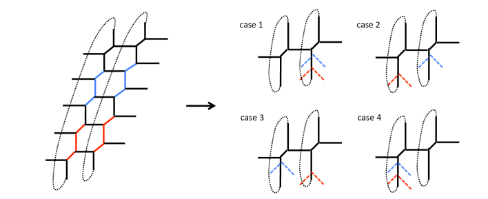
We start with the web diagram shown in Fig. 8.
Refer to caption
Figure 8: In this geometric transition we obtain the 𝖳𝖳\mathsf{T}-operator which consists of two 𝖸𝖸\mathsf{Y}-operators for A1subscript𝐴1A_{1} quiver. We set the Kähler parameters in the blue and red parts.

In this case we tune the following parameters to obtain two 𝖸𝖸\mathsf{Y}-operators,

Q2(1),Q3(1),Q2(2),Q3(2),superscriptsubscript𝑄21superscriptsubscript𝑄31superscriptsubscript𝑄22superscriptsubscript𝑄32\displaystyle Q_{2}^{(1)},~{}Q_{3}^{(1)},~{}Q_{2}^{(2)},~{}Q_{3}^{(2)}, (3.37a)
Q4(1),Q5(1),Q4(2),Q5(2).superscriptsubscript𝑄41superscriptsubscript𝑄51superscriptsubscript𝑄42superscriptsubscript𝑄52\displaystyle Q_{4}^{(1)},~{}Q_{5}^{(1)},~{}Q_{4}^{(2)},~{}Q_{5}^{(2)}. (3.37b)

The parameters (3.37a) and (3.37b) correspond to the blue brane and the red brane in Fig. 8, respectively. We show how to set the parameter in order to realize the brane configuration in each case:

Case 1::Case 1absent\displaystyle\text{\text@underline{Case 1}}:\ 𝖸(x1)𝖸(x2)𝖸subscript𝑥1𝖸subscript𝑥2\displaystyle\mathsf{Y}(x_{1})\mathsf{Y}(x_{2})
{Q2(1)=(q1q2)12,Q3(1)=(q1q2)12,Q4(1)=(q1q2)12,Q5(1)=(q1q2)12,Q2(2)=q1(q1q2)12,Q3(2)=q11(q1q2)12,Q4(2)=q1(q1q2)12,Q5(2)=q11(q1q2)12casesformulae-sequencesuperscriptsubscript𝑄21superscriptsubscript𝑞1subscript𝑞212formulae-sequencesuperscriptsubscript𝑄31superscriptsubscript𝑞1subscript𝑞212formulae-sequencesuperscriptsubscript𝑄41superscriptsubscript𝑞1subscript𝑞212superscriptsubscript𝑄51superscriptsubscript𝑞1subscript𝑞212otherwiseformulae-sequencesuperscriptsubscript𝑄22subscript𝑞1superscriptsubscript𝑞1subscript𝑞212formulae-sequencesuperscriptsubscript𝑄32superscriptsubscript𝑞11superscriptsubscript𝑞1subscript𝑞212formulae-sequencesuperscriptsubscript𝑄42subscript𝑞1superscriptsubscript𝑞1subscript𝑞212superscriptsubscript𝑄52superscriptsubscript𝑞11superscriptsubscript𝑞1subscript𝑞212otherwise\displaystyle\begin{cases}Q_{2}^{(1)}=(q_{1}q_{2})^{-\frac{1}{2}},~{}Q_{3}^{(1)}=(q_{1}q_{2})^{-\frac{1}{2}},~{}Q_{4}^{(1)}=(q_{1}q_{2})^{-\frac{1}{2}},~{}Q_{5}^{(1)}=(q_{1}q_{2})^{-\frac{1}{2}},\\ Q_{2}^{(2)}=q_{1}(q_{1}q_{2})^{-\frac{1}{2}},~{}Q_{3}^{(2)}=q_{1}^{-1}(q_{1}q_{2})^{-\frac{1}{2}},~{}Q_{4}^{(2)}=q_{1}(q_{1}q_{2})^{-\frac{1}{2}},~{}Q_{5}^{(2)}=q_{1}^{-1}(q_{1}q_{2})^{-\frac{1}{2}}\end{cases} (3.38a)
Case 2::Case 2absent\displaystyle\text{\text@underline{Case 2}}:\ 𝖸(x1)/𝖸(q1x2)𝖸subscript𝑥1𝖸superscript𝑞1subscript𝑥2\displaystyle\mathsf{Y}(x_{1})/\mathsf{Y}(q^{-1}x_{2})
{Q2(1)=(q1q2)12,Q3(1)=(q1q2)12,Q4(1)=q1(q1q2)12,Q5(1)=q11(q1q2)12,Q2(2)=q1(q1q2)12,Q3(2)=q11(q1q2)12,Q4(2)=(q1q2)12,Q5(2)=(q1q2)12casesformulae-sequencesuperscriptsubscript𝑄21superscriptsubscript𝑞1subscript𝑞212formulae-sequencesuperscriptsubscript𝑄31superscriptsubscript𝑞1subscript𝑞212formulae-sequencesuperscriptsubscript𝑄41subscript𝑞1superscriptsubscript𝑞1subscript𝑞212superscriptsubscript𝑄51superscriptsubscript𝑞11superscriptsubscript𝑞1subscript𝑞212otherwiseformulae-sequencesuperscriptsubscript𝑄22subscript𝑞1superscriptsubscript𝑞1subscript𝑞212formulae-sequencesuperscriptsubscript𝑄32superscriptsubscript𝑞11superscriptsubscript𝑞1subscript𝑞212formulae-sequencesuperscriptsubscript𝑄42superscriptsubscript𝑞1subscript𝑞212superscriptsubscript𝑄52superscriptsubscript𝑞1subscript𝑞212otherwise\displaystyle\begin{cases}Q_{2}^{(1)}=(q_{1}q_{2})^{-\frac{1}{2}},~{}Q_{3}^{(1)}=(q_{1}q_{2})^{-\frac{1}{2}},~{}Q_{4}^{(1)}=q_{1}(q_{1}q_{2})^{-\frac{1}{2}},~{}Q_{5}^{(1)}=q_{1}^{-1}(q_{1}q_{2})^{-\frac{1}{2}},\\ Q_{2}^{(2)}=q_{1}(q_{1}q_{2})^{-\frac{1}{2}},~{}Q_{3}^{(2)}=q_{1}^{-1}(q_{1}q_{2})^{-\frac{1}{2}},~{}Q_{4}^{(2)}=(q_{1}q_{2})^{\frac{1}{2}},~{}Q_{5}^{(2)}=(q_{1}q_{2})^{\frac{1}{2}}\end{cases} (3.38b)
Case 3::Case 3absent\displaystyle\text{\text@underline{Case 3}}:\ 𝖸(x2)/𝖸(q1x1)𝖸subscript𝑥2𝖸superscript𝑞1subscript𝑥1\displaystyle\mathsf{Y}(x_{2})/\mathsf{Y}(q^{-1}x_{1})
{Q2(1)=q1(q1q2)12,Q3(1)=q11(q1q2)12,Q4(1)=(q1q2)12,Q5(1)=(q1q2)12,Q2(2)=(q1q2)12,Q3(2)=(q1q2)12,Q4(2)=q1(q1q2)12,Q5(2)=q11(q1q2)12casesformulae-sequencesuperscriptsubscript𝑄21subscript𝑞1superscriptsubscript𝑞1subscript𝑞212formulae-sequencesuperscriptsubscript𝑄31superscriptsubscript𝑞11superscriptsubscript𝑞1subscript𝑞212formulae-sequencesuperscriptsubscript𝑄41superscriptsubscript𝑞1subscript𝑞212superscriptsubscript𝑄51superscriptsubscript𝑞1subscript𝑞212otherwiseformulae-sequencesuperscriptsubscript𝑄22superscriptsubscript𝑞1subscript𝑞212formulae-sequencesuperscriptsubscript𝑄32superscriptsubscript𝑞1subscript𝑞212formulae-sequencesuperscriptsubscript𝑄42subscript𝑞1superscriptsubscript𝑞1subscript𝑞212superscriptsubscript𝑄52superscriptsubscript𝑞11superscriptsubscript𝑞1subscript𝑞212otherwise\displaystyle\begin{cases}Q_{2}^{(1)}=q_{1}(q_{1}q_{2})^{-\frac{1}{2}},~{}Q_{3}^{(1)}=q_{1}^{-1}(q_{1}q_{2})^{-\frac{1}{2}},~{}Q_{4}^{(1)}=(q_{1}q_{2})^{-\frac{1}{2}},~{}Q_{5}^{(1)}=(q_{1}q_{2})^{-\frac{1}{2}},\\ Q_{2}^{(2)}=(q_{1}q_{2})^{\frac{1}{2}},~{}Q_{3}^{(2)}=(q_{1}q_{2})^{\frac{1}{2}},~{}Q_{4}^{(2)}=q_{1}(q_{1}q_{2})^{-\frac{1}{2}},~{}Q_{5}^{(2)}=q_{1}^{-1}(q_{1}q_{2})^{-\frac{1}{2}}\end{cases} (3.38c)
Case 4::Case 4absent\displaystyle\text{\text@underline{Case 4}}:\ (𝖸(q1x1)𝖸(q1x2))1superscript𝖸superscript𝑞1subscript𝑥1𝖸superscript𝑞1subscript𝑥21\displaystyle\left(\mathsf{Y}(q^{-1}x_{1})\mathsf{Y}(q^{-1}x_{2})\right)^{-1}
{Q2(1)=q1(q1q2)12,Q3(1)=q11(q1q2)12,Q4(1)=q1(q1q2)12,Q5(1)=q11(q1q2)12,Q2(2)=(q1q2)12,Q3(2)=(q1q2)12,Q4(2)=(q1q2)12,Q5(2)=(q1q2)12casesformulae-sequencesuperscriptsubscript𝑄21subscript𝑞1superscriptsubscript𝑞1subscript𝑞212formulae-sequencesuperscriptsubscript𝑄31superscriptsubscript𝑞11superscriptsubscript𝑞1subscript𝑞212formulae-sequencesuperscriptsubscript𝑄41subscript𝑞1superscriptsubscript𝑞1subscript𝑞212superscriptsubscript𝑄51superscriptsubscript𝑞11superscriptsubscript𝑞1subscript𝑞212otherwiseformulae-sequencesuperscriptsubscript𝑄22superscriptsubscript𝑞1subscript𝑞212formulae-sequencesuperscriptsubscript𝑄32superscriptsubscript𝑞1subscript𝑞212formulae-sequencesuperscriptsubscript𝑄42superscriptsubscript𝑞1subscript𝑞212superscriptsubscript𝑄52superscriptsubscript𝑞1subscript𝑞212otherwise\displaystyle\begin{cases}Q_{2}^{(1)}=q_{1}(q_{1}q_{2})^{-\frac{1}{2}},~{}Q_{3}^{(1)}=q_{1}^{-1}(q_{1}q_{2})^{-\frac{1}{2}},~{}Q_{4}^{(1)}=q_{1}(q_{1}q_{2})^{-\frac{1}{2}},~{}Q_{5}^{(1)}=q_{1}^{-1}(q_{1}q_{2})^{-\frac{1}{2}},\\ Q_{2}^{(2)}=(q_{1}q_{2})^{\frac{1}{2}},~{}Q_{3}^{(2)}=(q_{1}q_{2})^{\frac{1}{2}},~{}Q_{4}^{(2)}=(q_{1}q_{2})^{\frac{1}{2}},~{}Q_{5}^{(2)}=(q_{1}q_{2})^{\frac{1}{2}}\end{cases} (3.38d)

In the cases 2, 3, 4, we have to perform the q1q2subscript𝑞1subscript𝑞2q_{1}q_{2}-shift as before, where we define

Qx1:=Q1x1=(q1Q1(2)i=35Qτi(2))1=(q1i=35Qτi(1)),assignsubscript𝑄subscript𝑥1subscript𝑄1subscript𝑥1superscriptsubscript𝑞1superscriptsubscript𝑄12superscriptsubscriptproduct𝑖35subscriptsuperscript𝑄2subscript𝜏𝑖1subscript𝑞1superscriptsubscriptproduct𝑖35subscriptsuperscript𝑄1subscript𝜏𝑖\displaystyle Q_{x_{1}}:=\frac{Q_{1}}{x_{1}}=(q_{1}Q_{1}^{(2)}\prod_{i=3}^{5}Q^{(2)}_{\tau_{i}})^{-1}=(q_{1}\prod_{i=3}^{5}Q^{(1)}_{\tau_{i}}), (3.39a)
Qx2:=Q1x2=(q1Q1(2)Qτ5(2))1=(q1Qτ5(1))assignsubscript𝑄subscript𝑥2subscript𝑄1subscript𝑥2superscriptsubscript𝑞1superscriptsubscript𝑄12subscriptsuperscript𝑄2subscript𝜏51subscript𝑞1subscriptsuperscript𝑄1subscript𝜏5\displaystyle Q_{x_{2}}:=\frac{Q_{1}}{x_{2}}=(q_{1}Q_{1}^{(2)}Q^{(2)}_{\tau_{5}})^{-1}=(q_{1}Q^{(1)}_{\tau_{5}}) (3.39b)

Then the partition function 𝒵2,5subscript𝒵25\mathcal{Z}_{2,5} gives rise to the two-point function of the 𝖸𝖸\mathsf{Y}-operator, by multiplying the μ𝜇\mu-independent factor,

𝒵2,5{<𝖸(x1)𝖸(x2)>(case 1)𝖸(x1)𝖸(q1x2)(case 2)𝖸(x2)𝖸(q1x1)(case 3)(𝖸(q1x1)𝖸(q1x2))1(case 4)subscript𝒵25casesexpectation𝖸subscript𝑥1𝖸subscript𝑥2(case 1)delimited-⟨⟩𝖸subscript𝑥1𝖸superscript𝑞1subscript𝑥2(case 2)delimited-⟨⟩𝖸subscript𝑥2𝖸superscript𝑞1subscript𝑥1(case 3)delimited-⟨⟩superscript𝖸superscript𝑞1subscript𝑥1𝖸superscript𝑞1subscript𝑥21(case 4)\displaystyle\mathcal{Z}_{2,5}\ \longrightarrow\ \begin{cases}\Big{<}\mathsf{Y}(x_{1})\mathsf{Y}(x_{2})\Big{>}&\text{(case 1)}\\[10.00002pt] \displaystyle\left<\frac{\mathsf{Y}(x_{1})}{\mathsf{Y}(q^{-1}x_{2})}\right>&\text{(case 2)}\\[10.00002pt] \displaystyle\left<\frac{\mathsf{Y}(x_{2})}{\mathsf{Y}(q^{-1}x_{1})}\right>&\text{(case 3)}\\[10.00002pt] \displaystyle\left<\left(\mathsf{Y}(q^{-1}x_{1})\mathsf{Y}(q^{-1}x_{2})\right)^{-1}\right>&\text{(case 4)}\end{cases} (3.40)

where the average is taken with respect to the U(1) Nekrasov function (3.20). Then the average of the 𝖳𝖳\mathsf{T}-operator defined

χ\yng(2)(A1;q1,q2)subscript𝜒\yng2subscript𝐴1subscript𝑞1subscript𝑞2\displaystyle\chi_{\tiny\yng(2)}(A_{1};q_{1},q_{2}) =<𝖳[2](x1,x2)>absentexpectationsuperscript𝖳delimited-[]2subscript𝑥1subscript𝑥2\displaystyle=\Big{<}\mathsf{T}^{[2]}(x_{1},x_{2})\Big{>}
:=<𝖸(x1)𝖸(x2)>+𝔮𝖯(x1)𝖲(x2x1)𝖸(x2)𝖸(q1x1)assignabsentexpectation𝖸subscript𝑥1𝖸subscript𝑥2𝔮𝖯subscript𝑥1𝖲subscript𝑥2subscript𝑥1delimited-⟨⟩𝖸subscript𝑥2𝖸superscript𝑞1subscript𝑥1\displaystyle:=\Big{<}\mathsf{Y}(x_{1})\mathsf{Y}(x_{2})\Big{>}+\mathfrak{q}\,\mathsf{P}(x_{1})\mathsf{S}\left(\frac{x_{2}}{x_{1}}\right)\left<\frac{\mathsf{Y}(x_{2})}{\mathsf{Y}(q^{-1}x_{1})}\right>
+𝔮𝖯(x2)𝖲(x1x2)𝖸(x1)𝖸(q1x2)+𝔮2𝖯(x1)𝖯(x2)𝖸(q1x1)𝖸(q1x2)𝔮𝖯subscript𝑥2𝖲subscript𝑥1subscript𝑥2delimited-⟨⟩𝖸subscript𝑥1𝖸superscript𝑞1subscript𝑥2superscript𝔮2𝖯subscript𝑥1𝖯subscript𝑥2𝖸superscript𝑞1subscript𝑥1𝖸superscript𝑞1subscript𝑥2\displaystyle\hskip 30.00005pt+\mathfrak{q}\,\mathsf{P}(x_{2})\mathsf{S}\left(\frac{x_{1}}{x_{2}}\right)\left<\frac{\mathsf{Y}(x_{1})}{\mathsf{Y}(q^{-1}x_{2})}\right>+\mathfrak{q}^{2}\,\frac{\mathsf{P}(x_{1})\mathsf{P}(x_{2})}{\mathsf{Y}(q^{-1}x_{1})\mathsf{Y}(q^{-1}x_{2})} (3.41)

yields the qq𝑞𝑞qq-character of the degree-2 symmetric representation for A1subscript𝐴1A_{1} quiver, and its regularity is again shown using the iWeyl reflection (3.29). Now the 𝖲𝖲\mathsf{S}-factor is defined [26]

𝖲(x)𝖲𝑥\displaystyle\mathsf{S}(x) =θ1(q1x)θ1(q2x)θ1(qx)θ1(x)absentsubscript𝜃1subscript𝑞1𝑥subscript𝜃1subscript𝑞2𝑥subscript𝜃1𝑞𝑥subscript𝜃1𝑥\displaystyle=\frac{\theta_{1}(q_{1}x)\theta_{1}(q_{2}x)}{\theta_{1}(qx)\theta_{1}(x)} (3.42)

and the matter factor 𝖯(x)𝖯𝑥\mathsf{P}(x) is the same as (3.28). This qq𝑞𝑞qq-character is regular even in the collision limit x2x1subscript𝑥2subscript𝑥1x_{2}\to x_{1}, involving a derivative term, which is a specific feature to the qq𝑞𝑞qq-character [19]. In this limit, the cycle between the blue and red ones shrinks in Fig. 8. We show the proof of the regularity in Appendix B. We remark that we put the μ𝜇\mu-independent factors 𝖲(x)𝖲𝑥\mathsf{S}(x) and 𝖯(x)𝖯𝑥\mathsf{P}(x) to define the 𝖳𝖳\mathsf{T}-operator because it’s a matter of the normalization of the partition function.

In general, the n𝑛n-point function of the 𝖸𝖸\mathsf{Y}-operator for SU(N𝑁N) theory is obtained from the partition function 𝒵2,N+2nsubscript𝒵2𝑁2𝑛\mathcal{Z}_{2,N+2n} with 2nsuperscript2𝑛2^{n} possible brane insertions,

𝒵2,N+2n<𝖸(x1)𝖸(xn)>,𝖸(x2)𝖸(xn)𝖸(q1x1),𝖸(x3)𝖸(xn)𝖸(q1x1)𝖸(q1x2),subscript𝒵2𝑁2𝑛expectation𝖸subscript𝑥1𝖸subscript𝑥𝑛delimited-⟨⟩𝖸subscript𝑥2𝖸subscript𝑥𝑛𝖸superscript𝑞1subscript𝑥1delimited-⟨⟩𝖸subscript𝑥3𝖸subscript𝑥𝑛𝖸superscript𝑞1subscript𝑥1𝖸superscript𝑞1subscript𝑥2\displaystyle\mathcal{Z}_{2,N+2n}\ \longrightarrow\ \Big{<}\mathsf{Y}(x_{1})\cdots\mathsf{Y}(x_{n})\Big{>}\,,\ \left<\frac{\mathsf{Y}(x_{2})\cdots\mathsf{Y}(x_{n})}{\mathsf{Y}(q^{-1}x_{1})}\right>\,,\ \left<\frac{\mathsf{Y}(x_{3})\cdots\mathsf{Y}(x_{n})}{\mathsf{Y}(q^{-1}x_{1})\mathsf{Y}(q^{-1}x_{2})}\right>\,,\ldots (3.43)

We can construct the qq𝑞𝑞qq-character of the degree-n𝑛n representation Rn=nsubscript𝑅𝑛subscript𝑛R_{n}=\underbrace{\square\cdots\square}_{n} for A1subscript𝐴1A_{1} quiver by summing up all the possible n𝑛n-point functions of the 𝖸𝖸\mathsf{Y}-operator [19, 25, 26], with a suitable 𝖲𝖲\mathsf{S}-factor inserted,

χRn(A1;q1,q2)=<𝖳[n](x1,,xn)>subscript𝜒subscript𝑅𝑛subscript𝐴1subscript𝑞1subscript𝑞2expectationsuperscript𝖳delimited-[]𝑛subscript𝑥1subscript𝑥𝑛\displaystyle\chi_{R_{n}}(A_{1};q_{1},q_{2})=\Big{<}\mathsf{T}^{[n]}(x_{1},\ldots,x_{n})\Big{>} :=<𝖸(x1)𝖸(xn)>+.assignabsentexpectation𝖸subscript𝑥1𝖸subscript𝑥𝑛\displaystyle:=\Big{<}\mathsf{Y}(x_{1})\cdots\mathsf{Y}(x_{n})\Big{>}+\cdots\,. (3.44)

3.3 A2subscript𝐴2A_{2} quiver

Next we consider the A2subscript𝐴2A_{2} quiver gauge theory to examine the qq𝑞𝑞qq-character using the refined geometric transition. As mentioned in Sec. 3.1, the Seiberg–Witten curve and its quantization are associated with the fundamental representation character of GΓsubscript𝐺ΓG_{\Gamma}-group for ΓΓ\Gamma-quiver gauge theory. Thus in this case it is deeply related to the representation theory of SU(3) group. Since the qq𝑞𝑞qq-character generated by the iWeyl reflection does not depend on the gauge group rank, let us focus on the Abelian A2subscript𝐴2A_{2} quiver theory, U(1)×U(1)U1U1\mathrm{U}(1)\times\mathrm{U}(1), for simplicity. We have three possible ways to insert the defect brane as shown in Fig. 9.
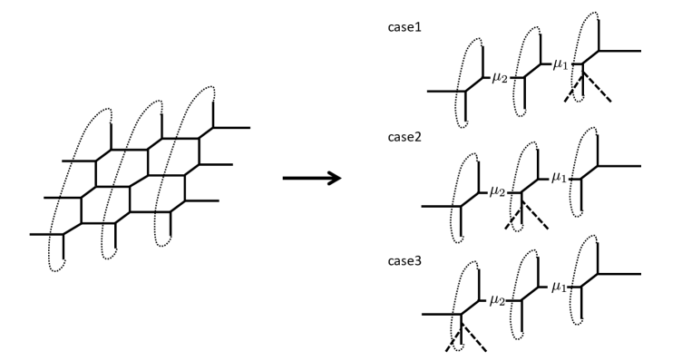
Refer to caption
Figure 9: In this geometric transition we obtain the 𝖳𝖳\mathsf{T}-operator for A2subscript𝐴2A_{2} quiver.

Case 1

We consider the defect brane inserted to the right-most NS5-brane. In this case, the calculation is essentially the same as that for A1subscript𝐴1A_{1} quiver shown in Fig. 5. We apply the following configuration

Q2(1)=Q3(1)=(q1q2)12,Q2(2)=Q3(2)=(q1q2)12,formulae-sequencesuperscriptsubscript𝑄21superscriptsubscript𝑄31superscriptsubscript𝑞1subscript𝑞212superscriptsubscript𝑄22superscriptsubscript𝑄32superscriptsubscript𝑞1subscript𝑞212\displaystyle Q_{2}^{(1)}=Q_{3}^{(1)}=(q_{1}q_{2})^{-\frac{1}{2}},~{}Q_{2}^{(2)}=Q_{3}^{(2)}=(q_{1}q_{2})^{-\frac{1}{2}},~{}
Q2(3)=q1(q1q2)12,Q3(3)=q11(q1q2)12,Qτ2(3)=q1q21,formulae-sequencesuperscriptsubscript𝑄23subscript𝑞1superscriptsubscript𝑞1subscript𝑞212formulae-sequencesuperscriptsubscript𝑄33superscriptsubscript𝑞11superscriptsubscript𝑞1subscript𝑞212superscriptsubscript𝑄subscript𝜏23subscript𝑞1superscriptsubscript𝑞21\displaystyle Q_{2}^{(3)}=q_{1}(q_{1}q_{2})^{-\frac{1}{2}},~{}Q_{3}^{(3)}=q_{1}^{-1}(q_{1}q_{2})^{-\frac{1}{2}},~{}Q_{\tau_{2}}^{(3)}=q_{1}q_{2}^{-1}, (3.45)

with the Coulomb moduli parameter

Q1,1x=(q1Q1(3)Qτ3(3))1.subscript𝑄11𝑥superscriptsubscript𝑞1superscriptsubscript𝑄13superscriptsubscript𝑄subscript𝜏331\displaystyle\frac{Q_{1,1}}{x}=(q_{1}Q_{1}^{(3)}Q_{\tau_{3}}^{(3)})^{-1}\,. (3.46)

Comparing with the 𝖸𝖸\mathsf{Y}-operator definition (3.15), the contribution of the defect brane leads to 𝖸1,μ2(x)subscript𝖸1subscript𝜇2𝑥\mathsf{Y}_{1,\mu_{2}}(x) by multiplying the factor θ1(Q1,1/x)subscript𝜃1subscript𝑄11𝑥\theta_{1}(Q_{1,1}/x). Thus the partition function 𝒵3,3subscript𝒵33\mathcal{Z}_{3,3} gives rise to the average of 𝖸1(x)subscript𝖸1𝑥\mathsf{Y}_{1}(x) under the parametrization (3.45):

𝒵3,3(3.45)<𝖸1(x)>superscriptitalic-(3.45italic-)subscript𝒵33expectationsubscript𝖸1𝑥\displaystyle\mathcal{Z}_{3,3}\ \stackrel{{\scriptstyle\eqref{eq:Y_parametrize_case1}}}{{\longrightarrow}}\ \Big{<}\mathsf{Y}_{1}(x)\Big{>} (3.47)

where the operator average is taken with respect to 6d U(1)×U(1)U1U1\mathrm{U}(1)\times\mathrm{U}(1) Nekrasov function

<𝒪(x)>expectation𝒪𝑥\displaystyle\Big{<}\mathcal{O}(x)\Big{>} =μ1,μ2𝒪μ1,μ2(x)𝒵μ1,μ2U(1)×U(1)absentsubscriptsubscript𝜇1subscript𝜇2subscript𝒪subscript𝜇1subscript𝜇2𝑥superscriptsubscript𝒵subscript𝜇1subscript𝜇2U1U1\displaystyle=\sum_{\mu_{1},\mu_{2}}\mathcal{O}_{\mu_{1},\mu_{2}}(x)\,\mathcal{Z}_{\mu_{1},\mu_{2}}^{\mathrm{U}(1)\times\mathrm{U}(1)} (3.48a)
𝒵μ1,μ2U(1)×U(1)superscriptsubscript𝒵subscript𝜇1subscript𝜇2U1U1\displaystyle\mathcal{Z}_{\mu_{1},\mu_{2}}^{\mathrm{U}(1)\times\mathrm{U}(1)} =Q¯f,1|μ1|Q¯f,2|μ2|(i,j)μ1θ1(Q1(3)1q2μ1,ijq1i1)θ1(Q1(2)1q2μ1,i+j1q1μ2,jti)θ1(q2μ1,i+jq1μ1,jti+1)θ1(q2μ1,i+j1q1μ1,jti)absentsuperscriptsubscript¯𝑄𝑓1subscript𝜇1superscriptsubscript¯𝑄𝑓2subscript𝜇2subscriptproduct𝑖𝑗subscript𝜇1subscript𝜃1superscriptsubscript𝑄1superscript31superscriptsubscript𝑞2subscript𝜇1𝑖𝑗superscriptsubscript𝑞1𝑖1subscript𝜃1superscriptsubscript𝑄1superscript21superscriptsubscript𝑞2subscript𝜇1𝑖𝑗1superscriptsubscript𝑞1superscriptsubscript𝜇2𝑗𝑡𝑖subscript𝜃1superscriptsubscript𝑞2subscript𝜇1𝑖𝑗superscriptsubscript𝑞1superscriptsubscript𝜇1𝑗𝑡𝑖1subscript𝜃1superscriptsubscript𝑞2subscript𝜇1𝑖𝑗1superscriptsubscript𝑞1superscriptsubscript𝜇1𝑗𝑡𝑖\displaystyle=\bar{Q}_{f,1}^{|\mu_{1}|}\bar{Q}_{f,2}^{|\mu_{2}|}\prod_{(i,j)\in\mu_{1}}\frac{\theta_{1}(Q_{1}^{(3)^{-1}}q_{2}^{\mu_{1,i}-j}q_{1}^{i-1})\theta_{1}(Q_{1}^{(2)^{-1}}q_{2}^{-\mu_{1,i}+j-1}q_{1}^{\mu_{2,j}^{t}-i})}{\theta_{1}(q_{2}^{-\mu_{1,i}+j}q_{1}^{\mu_{1,j}^{t}-i+1})\theta_{1}(q_{2}^{-\mu_{1,i}+j-1}q_{1}^{\mu_{1,j}^{t}-i})}
×(i,j)μ2θ1(Q1(2)1q2μ2,ijq1μ1,jt+i1)θ1(Q1(1)1q2μ2,i+j1q1i)θ1(q2μ2,i+jq1μ2,jti+1)θ1(q2μ2,i+j1q1μ2,jti),\displaystyle\qquad\times\prod_{(i,j)\in\mu_{2}}\frac{\theta_{1}(Q_{1}^{(2)^{-1}}q_{2}^{\mu_{2,i}-j}q_{1}^{-\mu_{1,j}^{t}+i-1})\theta_{1}(Q_{1}^{(1)^{-1}}q_{2}^{-\mu_{2,i}+j-1}q_{1}^{-i})}{\theta_{1}(q_{2}^{-\mu_{2,i}+j}q_{1}^{\mu_{2,j}^{t}-i+1})\theta_{1}(q_{2}^{-\mu_{2,i}+j-1}q_{1}^{\mu_{2,j}^{t}-i})}, (3.48b)

where we define the gauge couplings Q¯f,1,2subscript¯𝑄𝑓12\bar{Q}_{f,1,2} and the Young diagrams μ1,2subscript𝜇12\mu_{1,2} as follows,

Q¯f,1=Q¯f,1(2),Q¯f,2=Q¯f,1(1),formulae-sequencesubscript¯𝑄𝑓1superscriptsubscript¯𝑄𝑓12subscript¯𝑄𝑓2superscriptsubscript¯𝑄𝑓11\displaystyle\bar{Q}_{f,1}=\bar{Q}_{f,1}^{(2)},~{}\bar{Q}_{f,2}=\bar{Q}_{f,1}^{(1)}, (3.49)
μ1=μ1(2),μ2=μ1(1).formulae-sequencesubscript𝜇1superscriptsubscript𝜇12subscript𝜇2superscriptsubscript𝜇11\displaystyle\mu_{1}=\mu_{1}^{(2)},~{}\mu_{2}=\mu_{1}^{(1)}. (3.50)

Case 2

In this case, the defect brane is inserted to the middle brane. This configuration corresponds to the following parametrization

Q2(1)=Q3(1)=(q1q2)12,Q2(3)=Q3(3)=(q1q2)12,formulae-sequencesuperscriptsubscript𝑄21superscriptsubscript𝑄31superscriptsubscript𝑞1subscript𝑞212superscriptsubscript𝑄23superscriptsubscript𝑄33superscriptsubscript𝑞1subscript𝑞212\displaystyle Q_{2}^{(1)}=Q_{3}^{(1)}=(q_{1}q_{2})^{-\frac{1}{2}},~{}Q_{2}^{(3)}=Q_{3}^{(3)}=(q_{1}q_{2})^{\frac{1}{2}},~{}
Q2(2)=q1(q1q2)12,Q3(2)=q11(q1q2)12,Qτ2(3)=q1q21,formulae-sequencesuperscriptsubscript𝑄22subscript𝑞1superscriptsubscript𝑞1subscript𝑞212formulae-sequencesuperscriptsubscript𝑄32superscriptsubscript𝑞11superscriptsubscript𝑞1subscript𝑞212superscriptsubscript𝑄subscript𝜏23subscript𝑞1superscriptsubscript𝑞21\displaystyle Q_{2}^{(2)}=q_{1}(q_{1}q_{2})^{-\frac{1}{2}},~{}Q_{3}^{(2)}=q_{1}^{-1}(q_{1}q_{2})^{-\frac{1}{2}},~{}Q_{\tau_{2}}^{(3)}=q_{1}q_{2}^{-1}, (3.51)

and two Coulomb moduli parameters defined

Q1,1x=(q1Qτ3(2))1,Q2,1x=(q1Q1(2)Qτ3(2))1.formulae-sequencesubscript𝑄11𝑥superscriptsubscript𝑞1superscriptsubscript𝑄subscript𝜏321subscript𝑄21𝑥superscriptsubscript𝑞1superscriptsubscript𝑄12superscriptsubscript𝑄subscript𝜏321\displaystyle\frac{Q_{1,1}}{x}=(q_{1}Q_{\tau_{3}}^{(2)})^{-1}\,,\qquad\frac{Q_{2,1}}{x}=(q_{1}Q_{1}^{(2)}Q_{\tau_{3}}^{(2)})^{-1}\,. (3.52)

We remark that the difference between Q1,1subscript𝑄11Q_{1,1} and Q1,2subscript𝑄12Q_{1,2} is given by the factor Q1(2)=:QmQ_{1}^{(2)}=:Q_{m}, which is interpreted as the bifundamental mass parameter, because such a bifundamental mass can be absorbed by the shift of U(1) Coulomb moduli [24]. In this paper we do not explicitly write the bifundamental mass parameter.

In this case, the contribution of the Lagrange submanifolds reads

(i,j)μ1θ1(q2iq1j1Q2,1/x)θ1(q2i1q1jQ2,1/x)θ1(q2iq1jQ2,1/x)θ1(q2i1q1j1Q2,1/x)(i,j)μ2θ1(q2i1q1j1Q1,1/x)θ1(q2iq1jQ1,1/x)θ1(q2i+1q1jQ1,1/x)θ1(q2iq1j+1Q1,1/x).subscriptproduct𝑖𝑗subscript𝜇1subscript𝜃1superscriptsubscript𝑞2𝑖superscriptsubscript𝑞1𝑗1subscript𝑄21𝑥subscript𝜃1superscriptsubscript𝑞2𝑖1superscriptsubscript𝑞1𝑗subscript𝑄21𝑥subscript𝜃1superscriptsubscript𝑞2𝑖superscriptsubscript𝑞1𝑗subscript𝑄21𝑥subscript𝜃1superscriptsubscript𝑞2𝑖1superscriptsubscript𝑞1𝑗1subscript𝑄21𝑥subscriptproduct𝑖𝑗subscript𝜇2subscript𝜃1superscriptsubscript𝑞2𝑖1superscriptsubscript𝑞1𝑗1subscript𝑄11𝑥subscript𝜃1superscriptsubscript𝑞2𝑖superscriptsubscript𝑞1𝑗subscript𝑄11𝑥subscript𝜃1superscriptsubscript𝑞2𝑖1superscriptsubscript𝑞1𝑗subscript𝑄11𝑥subscript𝜃1superscriptsubscript𝑞2𝑖superscriptsubscript𝑞1𝑗1subscript𝑄11𝑥\displaystyle\prod_{(i,j)\in\mu_{1}}\frac{\theta_{1}(q_{2}^{i}q_{1}^{j-1}Q_{2,1}/x)\theta_{1}(q_{2}^{i-1}q_{1}^{j}Q_{2,1}/x)}{\theta_{1}(q_{2}^{i}q_{1}^{j}Q_{2,1}/x)\theta_{1}(q_{2}^{i-1}q_{1}^{j-1}Q_{2,1}/x)}\prod_{(i,j)\in\mu_{2}}\frac{\theta_{1}(q_{2}^{i-1}q_{1}^{j-1}Q_{1,1}/x)\theta_{1}(q_{2}^{i}q_{1}^{j}Q_{1,1}/x)}{\theta_{1}(q_{2}^{i+1}q_{1}^{j}Q_{1,1}/x)\theta_{1}(q_{2}^{i}q_{1}^{j+1}Q_{1,1}/x)}\,. (3.53)

In order to obtain a consistent result, we have to shift the parameters of the numerator in the second factor, as discussed in Sec. 2.3,

θ1(q2i1q1j1Q1,1/x)θ1(q2iq1jQ1,1/x)θ1(q2iq1jQ1,1/x)θ1(q2i+1q1j+1Q1,1/x).subscript𝜃1superscriptsubscript𝑞2𝑖1superscriptsubscript𝑞1𝑗1subscript𝑄11𝑥subscript𝜃1superscriptsubscript𝑞2𝑖superscriptsubscript𝑞1𝑗subscript𝑄11𝑥subscript𝜃1superscriptsubscript𝑞2𝑖superscriptsubscript𝑞1𝑗subscript𝑄11𝑥subscript𝜃1superscriptsubscript𝑞2𝑖1superscriptsubscript𝑞1𝑗1subscript𝑄11𝑥\displaystyle\theta_{1}(q_{2}^{i-1}q_{1}^{j-1}Q_{1,1}/x)\theta_{1}(q_{2}^{i}q_{1}^{j}Q_{1,1}/x)\ \longrightarrow\ \theta_{1}(q_{2}^{i}q_{1}^{j}Q_{1,1}/x)\theta_{1}(q_{2}^{i+1}q_{1}^{j+1}Q_{1,1}/x)\,. (3.54)

Multiplying the μ𝜇\mu-independent factors, θ1(Q2,1/x)subscript𝜃1subscript𝑄21𝑥\theta_{1}(Q_{2,1}/x) and θ1(qQ1,1/x)1subscript𝜃1superscript𝑞subscript𝑄11𝑥1\theta_{1}(qQ_{1,1}/x)^{-1}, the μ1subscript𝜇1\mu_{1}- and μ2subscript𝜇2\mu_{2}-contributions are written as 𝖸2(x)subscript𝖸2𝑥\mathsf{Y}_{2}(x) and 𝖸11(q1x)superscriptsubscript𝖸11superscript𝑞1𝑥\mathsf{Y}_{1}^{-1}(q^{-1}x), respectively. Thus the partition function 𝒵3,3subscript𝒵33\mathcal{Z}_{3,3} becomes the average of the 𝖸𝖸\mathsf{Y}-operator ratio, by tuning the parameters as (3.51),

𝒵3,3(3.51)𝖸2(x)𝖸1(q1x).superscriptitalic-(3.51italic-)subscript𝒵33delimited-⟨⟩subscript𝖸2𝑥subscript𝖸1superscript𝑞1𝑥\displaystyle\mathcal{Z}_{3,3}\ \stackrel{{\scriptstyle\eqref{eq:Y_parametrize_case2}}}{{\longrightarrow}}\ \left<\frac{\mathsf{Y}_{2}(x)}{\mathsf{Y}_{1}(q^{-1}x)}\right>\,. (3.55)

The average is again taken with respect to the U(1) ×\times U(1) Nekrasov function (3.48).

Case 3

The remaining situation is that the defect brane is inserted to the left-most brane. In this case, the calculation is essentially the same as Fig. 6 for A1subscript𝐴1A_{1} quiver theory. Applying the parametrization

Q2(2)=Q3(2)=(q1q2)12,Q2(3)=Q3(3)=(q1q2)12,formulae-sequencesuperscriptsubscript𝑄22superscriptsubscript𝑄32superscriptsubscript𝑞1subscript𝑞212superscriptsubscript𝑄23superscriptsubscript𝑄33superscriptsubscript𝑞1subscript𝑞212\displaystyle Q_{2}^{(2)}=Q_{3}^{(2)}=(q_{1}q_{2})^{\frac{1}{2}},~{}Q_{2}^{(3)}=Q_{3}^{(3)}=(q_{1}q_{2})^{\frac{1}{2}},~{}
Q2(1)=q1(q1q2)12,Q3(1)=q11(q1q2)12,Qτ2(3)=q1q21,formulae-sequencesuperscriptsubscript𝑄21subscript𝑞1superscriptsubscript𝑞1subscript𝑞212formulae-sequencesuperscriptsubscript𝑄31superscriptsubscript𝑞11superscriptsubscript𝑞1subscript𝑞212superscriptsubscript𝑄subscript𝜏23subscript𝑞1superscriptsubscript𝑞21\displaystyle Q_{2}^{(1)}=q_{1}(q_{1}q_{2})^{-\frac{1}{2}},~{}Q_{3}^{(1)}=q_{1}^{-1}(q_{1}q_{2})^{-\frac{1}{2}},~{}Q_{\tau_{2}}^{(3)}=q_{1}q_{2}^{-1},
Q2,1x=(q1Q1(2)Qτ3(1))1subscript𝑄21𝑥superscriptsubscript𝑞1superscriptsubscript𝑄12superscriptsubscript𝑄subscript𝜏311\displaystyle\frac{Q_{2,1}}{x}=(q_{1}Q_{1}^{(2)}Q_{\tau_{3}}^{(1)})^{-1} (3.56)

with a suitable q1q2subscript𝑞1subscript𝑞2q_{1}q_{2}-shift of the arguments to be consistent with the geometric transition, the partition function 𝒵3,3subscript𝒵33\mathcal{Z}_{3,3} yields

𝒵3,3(3.56)1𝖸2(q1x).superscriptitalic-(3.56italic-)subscript𝒵33delimited-⟨⟩1subscript𝖸2superscript𝑞1𝑥\displaystyle\mathcal{Z}_{3,3}\ \stackrel{{\scriptstyle\eqref{eq:Y_parametrize_case3}}}{{\longrightarrow}}\ \left<\frac{1}{\mathsf{Y}_{2}(q^{-1}x)}\right>\,. (3.57)

qq𝑞𝑞qq-characters

Now we can construct the qq𝑞𝑞qq-character using all the possible brane insertions. The qq𝑞𝑞qq-character of the fundamental representation for A2subscript𝐴2A_{2} quiver theory, denoted by 3, is given by the 𝖳𝖳\mathsf{T}-operator average,

χ3(A2;q1,q2)subscript𝜒3subscript𝐴2subscript𝑞1subscript𝑞2\displaystyle\chi_{\textbf{3}}(A_{2};q_{1},q_{2}) =<𝖳1(x)>absentexpectationsubscript𝖳1𝑥\displaystyle=\Big{<}\mathsf{T}_{1}(x)\Big{>}
:=<𝖸1(x)>+𝔮1𝖯1(x)𝖸2(x)𝖸1(q1x)+𝔮1𝔮2𝖯1(x)𝖯2(x)1𝖸2(q1x)assignabsentexpectationsubscript𝖸1𝑥subscript𝔮1subscript𝖯1𝑥delimited-⟨⟩subscript𝖸2𝑥subscript𝖸1superscript𝑞1𝑥subscript𝔮1subscript𝔮2subscript𝖯1𝑥subscript𝖯2𝑥delimited-⟨⟩1subscript𝖸2superscript𝑞1𝑥\displaystyle:=\Big{<}\mathsf{Y}_{1}(x)\Big{>}+\mathfrak{q}_{1}\,\mathsf{P}_{1}(x)\left<\frac{\mathsf{Y}_{2}(x)}{\mathsf{Y}_{1}(q^{-1}x)}\right>+\mathfrak{q}_{1}\mathfrak{q}_{2}\,\mathsf{P}_{1}(x)\mathsf{P}_{2}(x)\left<\frac{1}{\mathsf{Y}_{2}(q^{-1}x)}\right> (3.58)

where the coupling constants are given by 𝔮1=Q¯f,1subscript𝔮1subscript¯𝑄𝑓1\mathfrak{q}_{1}=\bar{Q}_{f,1} and 𝔮2=Q¯f,2subscript𝔮2subscript¯𝑄𝑓2\mathfrak{q}_{2}=\bar{Q}_{f,2}, and the matter factors are defined

𝖯1(x)=θ1(q1Q1(3)1Q1,11x),𝖯2(x)=θ1(Q1(1)1Q1(2)1Q1,1/x).formulae-sequencesubscript𝖯1𝑥subscript𝜃1superscript𝑞1superscriptsubscript𝑄1superscript31superscriptsubscript𝑄111𝑥subscript𝖯2𝑥subscript𝜃1superscriptsubscript𝑄1superscript11superscriptsubscript𝑄1superscript21subscript𝑄11𝑥\displaystyle\mathsf{P}_{1}(x)=\theta_{1}(q^{-1}Q_{1}^{(3)^{-1}}Q_{1,1}^{-1}x)\,,\qquad\mathsf{P}_{2}(x)=\theta_{1}(Q_{1}^{(1)^{-1}}Q_{1}^{(2)^{-1}}Q_{1,1}/x)\,. (3.59)

Although each factor in (3.58) has pole singularities as before, the qq𝑞𝑞qq-character itself is a regular entire function in x𝑥x, as shown in Appendix B. The local pole cancellation is performed by the iWeyl reflection

𝖸1(x)𝔮1𝖯1(x)𝖸2(x)𝖸1(q1x),𝖸2(x)𝔮2𝖯2(x)𝖸1(q1x)𝖸2(q1x).formulae-sequencesubscript𝖸1𝑥subscript𝔮1subscript𝖯1𝑥subscript𝖸2𝑥subscript𝖸1superscript𝑞1𝑥subscript𝖸2𝑥subscript𝔮2subscript𝖯2𝑥subscript𝖸1superscript𝑞1𝑥subscript𝖸2superscript𝑞1𝑥\displaystyle\mathsf{Y}_{1}(x)\ \longrightarrow\ \mathfrak{q}_{1}\,\mathsf{P}_{1}(x)\frac{\mathsf{Y}_{2}(x)}{\mathsf{Y}_{1}(q^{-1}x)}\,,\quad\mathsf{Y}_{2}(x)\ \longrightarrow\ \mathfrak{q}_{2}\,\mathsf{P}_{2}(x)\frac{\mathsf{Y}_{1}(q^{-1}x)}{\mathsf{Y}_{2}(q^{-1}x)}\,. (3.60)

For A2subscript𝐴2A_{2} quiver, we have another representation, which is the anti-fundamental representation denoted by 3¯¯3\bar{\textbf{3}}. The corresponding qq𝑞𝑞qq-character is generated by applying the iWeyl reflection (3.60) to the highest weight 𝖸2(x)subscript𝖸2𝑥\mathsf{Y}_{2}(x),

χ3¯(A2;q1,q2)subscript𝜒¯3subscript𝐴2subscript𝑞1subscript𝑞2\displaystyle\chi_{\bar{\textbf{3}}}(A_{2};q_{1},q_{2}) =<𝖳2(x)>absentexpectationsubscript𝖳2𝑥\displaystyle=\Big{<}\mathsf{T}_{2}(x)\Big{>}
:=<𝖸2(x)>+𝔮2𝖯2(x)𝖸1(q1x)𝖸2(q1x)+𝔮1𝔮2𝖯1(q1x)𝖯2(x)1𝖸1(q2x).assignabsentexpectationsubscript𝖸2𝑥subscript𝔮2subscript𝖯2𝑥delimited-⟨⟩subscript𝖸1superscript𝑞1𝑥subscript𝖸2superscript𝑞1𝑥subscript𝔮1subscript𝔮2subscript𝖯1superscript𝑞1𝑥subscript𝖯2𝑥delimited-⟨⟩1subscript𝖸1superscript𝑞2𝑥\displaystyle:=\Big{<}\mathsf{Y}_{2}(x)\Big{>}+\mathfrak{q}_{2}\,\mathsf{P}_{2}(x)\left<\frac{\mathsf{Y}_{1}(q^{-1}x)}{\mathsf{Y}_{2}(q^{-1}x)}\right>+\mathfrak{q}_{1}\mathfrak{q}_{2}\,\mathsf{P}_{1}(q^{-1}x)\mathsf{P}_{2}(x)\left<\frac{1}{\mathsf{Y}_{1}(q^{-2}x)}\right>\,. (3.61)

We remark that the operator 𝖸2(x)subscript𝖸2𝑥\mathsf{Y}_{2}(x) itself cannot be constructed by a single insertion of the defect brane, but is realized as a composite operator:

𝖸2(x)=𝖸1(q1x)×𝖸2(x)𝖸1(q1x).subscript𝖸2𝑥subscript𝖸1superscript𝑞1𝑥subscript𝖸2𝑥subscript𝖸1superscript𝑞1𝑥\displaystyle\mathsf{Y}_{2}(x)=\mathsf{Y}_{1}(q^{-1}x)\times\frac{\mathsf{Y}_{2}(x)}{\mathsf{Y}_{1}(q^{-1}x)}\,. (3.62)

In other words, the operator 𝖸2(x)subscript𝖸2𝑥\mathsf{Y}_{2}(x) is obtained by two insertions of the defect branes to the right-most and the middle branes (see the case 1 in Fig. 10).
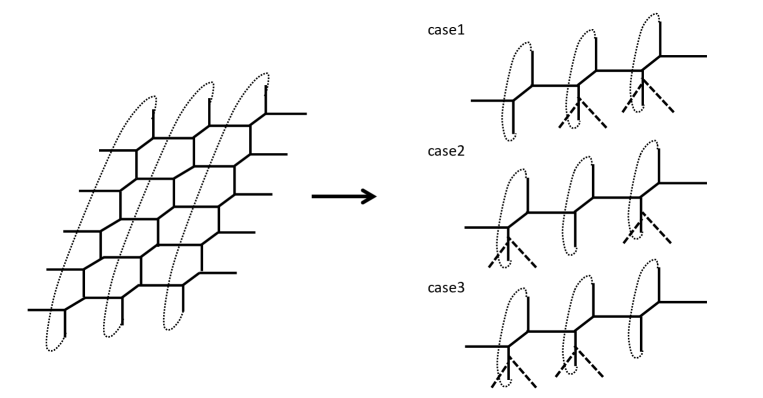
Refer to caption
Figure 10: The geometric transition which emerge the two defect branes. The summation of them corresponds to the qq𝑞𝑞qq-character of 𝟑¯¯3\bar{\bf{3}}.

Similarly the remaining terms in (3.61) are obtained as

𝖸1(q1x)𝖸2(q1x)=𝖸1(q1x)×1𝖸2(q1x)(case 2)subscript𝖸1superscript𝑞1𝑥subscript𝖸2superscript𝑞1𝑥subscript𝖸1superscript𝑞1𝑥1subscript𝖸2superscript𝑞1𝑥case 2\displaystyle\frac{\mathsf{Y}_{1}(q^{-1}x)}{\mathsf{Y}_{2}(q^{-1}x)}=\mathsf{Y}_{1}(q^{-1}x)\times\frac{1}{\mathsf{Y}_{2}(q^{-1}x)}\quad(\text{case 2}) (3.63)
1𝖸1(q2x)=𝖸2(q1x)𝖸1(q2x)×1𝖸2(q1x)(case 3)1subscript𝖸1superscript𝑞2𝑥subscript𝖸2superscript𝑞1𝑥subscript𝖸1superscript𝑞2𝑥1subscript𝖸2superscript𝑞1𝑥case 3\displaystyle\frac{1}{\mathsf{Y}_{1}(q^{-2}x)}=\frac{\mathsf{Y}_{2}(q^{-1}x)}{\mathsf{Y}_{1}(q^{-2}x)}\times\frac{1}{\mathsf{Y}_{2}(q^{-1}x)}\quad(\text{case 3}) (3.64)

Thus the qq𝑞𝑞qq-character of 3¯¯3\bar{\textbf{3}} for A2subscript𝐴2A_{2} quiver is given by summing all the possible configurations with two defect branes shown in Fig. 10.

3.4 Generic quiver

The argument discussed above is extended to generic (simply-laced) quiver gauge theory.

3.4.1 Arsubscript𝐴𝑟A_{r} quiver

For Arsubscript𝐴𝑟A_{r} quiver, there exist r𝑟r weights, associated with the gauge nodes, and the fundamental representation is obtained from each (highest) weight, which is the antisymmetric representation of SU(r+1𝑟1r+1). The qq𝑞𝑞qq-character of the degree n𝑛n antisymmetric representation Rnsuperscriptsubscript𝑅𝑛R_{n}^{\prime} (n=1,,r𝑛1𝑟n=1,\ldots,r) is given by [19]

χRn(Ar;q1,q2)subscript𝜒subscriptsuperscript𝑅𝑛subscript𝐴𝑟subscript𝑞1subscript𝑞2\displaystyle\chi_{R^{\prime}_{n}}(A_{r};q_{1},q_{2}) =<𝖳n(x)>absentexpectationsubscript𝖳𝑛𝑥\displaystyle=\Big{<}\mathsf{T}_{n}(x)\Big{>}
:=(k=1n𝔔k)1𝖯1(qnx)1i1<<inr+1k=1nΛik(qn+kx)assignabsentsuperscriptsuperscriptsubscriptproduct𝑘1𝑛subscript𝔔𝑘1subscript𝖯1superscript𝑞𝑛𝑥subscript1subscript𝑖1subscript𝑖𝑛𝑟1delimited-⟨⟩superscriptsubscriptproduct𝑘1𝑛subscriptΛsubscript𝑖𝑘superscript𝑞𝑛𝑘𝑥\displaystyle:=\left(\prod_{k=1}^{n}\mathfrak{Q}_{k}\right)^{-1}\mathsf{P}_{1}(q^{-n}x)\sum_{1\leq i_{1}<\cdots<i_{n}\leq r+1}\left<\prod_{k=1}^{n}\Lambda_{i_{k}}(q^{-n+k}x)\right>
=<𝖸n(x)>+𝔮n𝖸n1(q1x)𝖸n+1(x)𝖸n(q1x)+absentexpectationsubscript𝖸𝑛𝑥subscript𝔮𝑛delimited-⟨⟩subscript𝖸𝑛1superscript𝑞1𝑥subscript𝖸𝑛1𝑥subscript𝖸𝑛superscript𝑞1𝑥\displaystyle=\Big{<}\mathsf{Y}_{n}(x)\Big{>}+\mathfrak{q}_{n}\left<\frac{\mathsf{Y}_{n-1}(q^{-1}x)\mathsf{Y}_{n+1}(x)}{\mathsf{Y}_{n}(q^{-1}x)}\right>+\cdots (3.65)

where 𝔮nsubscript𝔮𝑛\mathfrak{q}_{n} is the gauge coupling of the n𝑛n-th gauge node, and we define

Λi(x)subscriptΛ𝑖𝑥\displaystyle\Lambda_{i}(x) =𝔔i𝖸i(x)𝖸i1(q1x)absentsubscript𝔔𝑖subscript𝖸𝑖𝑥subscript𝖸𝑖1superscript𝑞1𝑥\displaystyle=\mathfrak{Q}_{i}\,\frac{\mathsf{Y}_{i}(x)}{\mathsf{Y}_{i-1}(q^{-1}x)} (3.66)

with 𝖸0(x)=𝖯1(x)subscript𝖸0𝑥subscript𝖯1𝑥\mathsf{Y}_{0}(x)=\mathsf{P}_{1}(x), 𝖸r+1(x)=𝖯r(x)subscript𝖸𝑟1𝑥subscript𝖯𝑟𝑥\mathsf{Y}_{r+1}(x)=\mathsf{P}_{r}(x) and

𝔔i=k=1i1𝔮k.subscript𝔔𝑖superscriptsubscriptproduct𝑘1𝑖1subscript𝔮𝑘\displaystyle\mathfrak{Q}_{i}=\prod_{k=1}^{i-1}\mathfrak{q}_{k}\,. (3.67)

We can see that the qq𝑞𝑞qq-character is generated by the iWeyl reflection

𝖸n(x)𝔮n𝖸n1(q1x)𝖸n+1(x)𝖸n(q1x).subscript𝖸𝑛𝑥subscript𝔮𝑛subscript𝖸𝑛1superscript𝑞1𝑥subscript𝖸𝑛1𝑥subscript𝖸𝑛superscript𝑞1𝑥\displaystyle\mathsf{Y}_{n}(x)\ \longrightarrow\ \mathfrak{q}_{n}\,\frac{\mathsf{Y}_{n-1}(q^{-1}x)\mathsf{Y}_{n+1}(x)}{\mathsf{Y}_{n}(q^{-1}x)}\,. (3.68)

In this case there are r+1𝑟1r+1 NS5-branes, so that r+1𝑟1r+1 possibilities for the brane insertion. Indeed the factor Λi(x)subscriptΛ𝑖𝑥\Lambda_{i}(x) defined as (3.66) corresponds to the insertion of single defect brane. Thus the qq𝑞𝑞qq-character of Rnsuperscriptsubscript𝑅𝑛R_{n}^{\prime} is realized as the summation of all the possible configurations with n𝑛n brane insertions, since it involves a product of n𝑛n ΛΛ\Lambda-factors as shown in (3.65).

3.4.2 DE𝐷𝐸DE quiver

Let us then discuss DE𝐷𝐸DE quiver theory. In this case, it is not straightforwardly possible to obtain the toric Calabi–Yau threefold reproducing DE𝐷𝐸DE quiver gauge theory, due to the trivalent node in the quiver. Recently it has been proposed that DE𝐷𝐸DE-type gauge theory can be constructed from the (non-toric) Calabi–Yau geometry [57], and thus it is expected that we can discuss the qq𝑞𝑞qq-character by inserting the defect brane to such a DE𝐷𝐸DE-type configuration.

The simplest non-trivial DE𝐷𝐸DE-type theory is D4subscript𝐷4D_{4} quiver. In this case there are four fundamental representations corresponding to the nodes in D4subscript𝐷4D_{4} quiver, three 8-dimensional and one 28-dimensional representations. The three 8-representations are essentially equivalent to each other, which is so-called the SO(8) triality. In particular, for the 28-representation, the corresponding qq𝑞𝑞qq-character involves a derivative term, due to the collision limit of the 𝖸𝖸\mathsf{Y}-operators [19, 27], corresponding to the vanishing cycle as discussed in Sec. 3.2.3, and it would be interesting to study the geometric meaning of the collision limit.

3.4.3 Beyond ADE𝐴𝐷𝐸ADE quiver

For ADE𝐴𝐷𝐸ADE quiver, all the fundamental representations are finite dimensional, and thus the (qq𝑞𝑞qq-)character is given by a finite (elementary symmetric) polynomial of {Λi}subscriptΛ𝑖\{\Lambda_{i}\}, which is a ratio of the 𝖸𝖸\mathsf{Y}-operator (3.66). In general, we can consider the quiver, which does not correspond to the finite ADE𝐴𝐷𝐸ADE-type Dynkin diagram, namely affine and hyperbolic quivers. Although, in such a case, the fundamental representations become infinite dimensional, we can discuss the qq𝑞𝑞qq-character generated by the iWeyl reflection. For example, the affine quiver A^rsubscript^𝐴𝑟\hat{A}_{r} is realized using the infinitely-long linear quiver Asubscript𝐴A_{\infty} by imposing periodicity. Thus there are infinitely many possibilities for the brane insertion. This is a geometric interpretation of the infinite sum in the affine qq𝑞𝑞qq-character. For the simplest case A^0subscript^𝐴0\hat{A}_{0} corresponding to 4d 𝒩=2𝒩superscript2\mathcal{N}=2^{*} (5d 𝒩=1𝒩superscript1\mathcal{N}=1^{*}) theory, the qq𝑞𝑞qq-character is described as a summation over the partition [19, 25].

4 Summary and Discussion

In this paper, we have proposed the prescription of the geometric transition in the refined topological string enforced along the preferred direction. In order to obtain a proper contribution of the brane insertion, in addition to the specialization of the Kähler moduli, we have to shift the variable by hand to satisfy consistency, which becomes trivial in the unrefined limit. We then have applied this prescription to the codimension-4 defect operator, called the 𝖸𝖸\mathsf{Y}-operator as its stringy realization. The pole singularity of the 𝖸𝖸\mathsf{Y}-operator is cancelled out in a proper combination of the 𝖸𝖸\mathsf{Y}-operators, which is given by the qq𝑞𝑞qq-character. We have examined the pole cancellation in the qq𝑞𝑞qq-character as a nontrivial check of our prescription of the refined geometric transition.

Let us finally provide several open questions which we would like to resolve. As commented, the refined large N𝑁N duality between the resolved and deformed conifold has been clarified in terms of the refined Chern–Simons theory [15]. Nevertheless, the corresponding brane configuration is not clear from their argument, and as the first issue, we would pursue that our geometric transition may give a actual brane picture compatible with their result. Second, it may be possible that our prescription in Section 2.2 is generalized so as to incorporate the labels (p,q)𝑝𝑞(p,q) of the fivebrane charges, as mentioned there. The third thing is concerned with the exact definition of the refined version of the open topological vertex formalism. As far as we know, it is not yet established, and thus, the direct computation of the open string amplitude respecting the Lagrangian brane on the inner brane is still a nontrivial problem. In the unrefined case, the Schur function is suitable to capture the holonomy of D-branes corresponding to the insertion of the Lagrangian brane. It is expected from the results of [15] that the Schur function would be replaced with the Macdonald function in the refined case as done for the refined topological vertex in [10]. Combining the expression obtained via the refined geometric transition, we hope that the successful direct approach would be reported in the near future.

We also hold some technical and qualitative issues on the 𝖸𝖸\mathsf{Y}-operator. In the topological string approach, there is an ambiguity of the normalization. Actually the 𝖸𝖸\mathsf{Y}-operator and the qq𝑞𝑞qq-character have factors independent of the partition μ𝜇\mu, and we need to add such a factor by hand to obtain a proper result. It would be interesting to clarify a systematic way to discuss the μ𝜇\mu-independent factor in the framework of refined topological string.

The brane configuration of the 𝖸𝖸\mathsf{Y}-operator proposed in this paper is due to the comparison with the gauge theory definition. The current construction of the codimension-4 𝖸𝖸\mathsf{Y}-operator uses the codimension-2 surface defects with the q𝑞q-brane and anti-q𝑞q-brane. Such a relation between defect operators with different codimensions is not yet obvious. One possible interpretation is the tachyon condensation, which could be related to the (refined) supergroup Chern–Simons theory [41]. For example, it is interesting to compare the Y-operator contribution with the partition function of the refined U(1|||1) Chern–Simons theory [58]. More detailed analysis is necessary for understanding its geometric meaning in refined theory.

Acknowledgments

We would like to thank Shamil Shakirov, Masato Taki, Satoshi Yamaguchi, and Yegor Zenkevich for giving helpful comments. The work of T. K. was supported in part by Keio Gijuku Academic Development Funds, JSPS Grant-in-Aid for Scientific Research (No. JP17K18090), the MEXT-Supported Program for the Strategic Research Foundation at Private Universities “Topological Science” (No. S1511006), and JSPS Grant-in-Aid for Scientific Research on Innovative Areas “Topological Materials Science” (No. JP15H05855). The work of H. M. and Y. S. was supported in part by the JSPS Research Fellowship for Young Scientists.

Appendix A Definitions and notations

A.1 Mathematical preliminaries

Young diagram

To define the Young diagram, we take the decreasing sequence of nonnegative integers that is regularly used for the instanton counting problem. Let (i,j)𝑖𝑗(i,j) be positions of boxes in the diagram (shown in Fig. 11(a)), then we denote as μ𝜇\mu a Young diagram of the following set of l𝑙l-tuple diagrams (Fig. 11(b)):

μ𝜇\displaystyle\mu ={μi0|μ1μ2μl},absentconditional-setsubscript𝜇𝑖subscriptabsent0subscript𝜇1subscript𝜇2subscript𝜇𝑙\displaystyle=\left\{\mu_{i}\in\mathbb{Z}_{\geq 0}|\mu_{1}\geq\mu_{2}\geq\cdots\geq\mu_{l}\right\}, μtsuperscript𝜇𝑡\displaystyle\mu^{t} ={μjt0|μjt=#{i|μij}},absentconditional-setsuperscriptsubscript𝜇𝑗𝑡subscriptabsent0superscriptsubscript𝜇𝑗𝑡#conditional-set𝑖subscript𝜇𝑖𝑗\displaystyle=\left\{\mu_{j}^{t}\in\mathbb{Z}_{\geq 0}|\mu_{j}^{t}=\#\{i|\mu_{i}\geq j\}\right\}, (A.1)

where the transpose of μ𝜇\mu is indicated by the superscript t𝑡t (Fig. 11(c)). For a given Young diagram μ𝜇\mu, we use the following simplified symbols:

|μ|𝜇\displaystyle|\mu| =i=1lμi,absentsuperscriptsubscript𝑖1𝑙subscript𝜇𝑖\displaystyle=\sum_{i=1}^{l}\mu_{i}, μ2superscriptnorm𝜇2\displaystyle||\mu||^{2} =i=1lμi2,absentsuperscriptsubscript𝑖1𝑙superscriptsubscript𝜇𝑖2\displaystyle=\sum_{i=1}^{l}\mu_{i}^{2}, (i,j)μf(i,j)subscriptproduct𝑖𝑗𝜇𝑓𝑖𝑗\displaystyle\prod_{(i,j)\in\mu}f(i,j) =i=1lj=1μif(i,j).absentsuperscriptsubscriptproduct𝑖1𝑙superscriptsubscriptproduct𝑗1subscript𝜇𝑖𝑓𝑖𝑗\displaystyle=\prod_{i=1}^{l}\prod_{j=1}^{\mu_{i}}f(i,j). (A.2)

The first one in (A.2) is the total number of boxes of μ𝜇\mu. The partitions {μi}subscript𝜇𝑖\{\mu_{i}\} and {μjt}superscriptsubscript𝜇𝑗𝑡\{\mu_{j}^{t}\} concretely characterize the instanton partition function, which can be removed by using

j=1μi(μij)=j=1μi(j1)for fixed i,i=1μjt(μjti)=i=1μjt(i1)for fixed j.superscriptsubscript𝑗1subscript𝜇𝑖subscript𝜇𝑖𝑗absentsuperscriptsubscript𝑗1subscript𝜇𝑖𝑗1missing-subexpressionfor fixed isuperscriptsubscript𝑖1superscriptsubscript𝜇𝑗𝑡superscriptsubscript𝜇𝑗𝑡𝑖absentsuperscriptsubscript𝑖1superscriptsubscript𝜇𝑗𝑡𝑖1missing-subexpressionfor fixed j\displaystyle\begin{aligned} \sum_{j=1}^{\mu_{i}}\left(\mu_{i}-j\right)&=\sum_{j=1}^{\mu_{i}}\left(j-1\right)&&\text{for fixed $i$},\\ \sum_{i=1}^{\mu_{j}^{t}}\left(\mu_{j}^{t}-i\right)&=\sum_{i=1}^{\mu_{j}^{t}}\left(i-1\right)&&\text{for fixed $j$}.\end{aligned} (A.3)

In the paper, these are implicitly applied as expressing the 𝖸𝖸\mathsf{Y}-operator in a convenient fashion from the general form obtained via the refined geometric transition in Section 2.2.
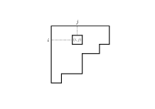
Refer to caption (a) Positions of boxes Refer to caption (b) l𝑙l-tuple diagram Refer to caption (c) Transpose
Figure 11: The Young diagram and its parameters.

Theta function

The topological string amplitude for the compactified web diagram of our interest is nicely expressed in terms of the theta function,

θ1(z|τ)=ieπiτ4eπizk=1(1e2πikτ)(1e2πikτe2πiz)(1e2πi(k1)τe2πiz),subscript𝜃1conditional𝑧𝜏𝑖superscript𝑒𝜋i𝜏4superscript𝑒𝜋i𝑧superscriptsubscriptproduct𝑘11superscript𝑒2𝜋i𝑘𝜏1superscript𝑒2𝜋i𝑘𝜏superscript𝑒2𝜋𝑖𝑧1superscript𝑒2𝜋i𝑘1𝜏superscript𝑒2𝜋i𝑧\displaystyle\theta_{1}(z|\tau)=-ie^{\pi\mathrm{i}\tau\over 4}e^{\pi\mathrm{i}z}\prod_{k=1}^{\infty}\left(1-e^{2\pi\mathrm{i}k\tau}\right)\left(1-e^{2\pi\mathrm{i}k\tau}e^{2\pi iz}\right)\left(1-e^{2\pi\mathrm{i}(k-1)\tau}e^{-2\pi\mathrm{i}z}\right), (A.4)

where a variable is z𝑧z\in\mathbb{C}, and τ𝜏\tau\in\mathbb{C} is a constant with Im(τ)>0Im𝜏0\text{Im}(\tau)>0. Equivalently, the theta function is frequently used in the multiplicative form,

θ1(x;q)=iq18x12(q,qx,x1;q),subscript𝜃1𝑥𝑞isuperscript𝑞18superscript𝑥12subscript𝑞𝑞𝑥superscript𝑥1𝑞\displaystyle\theta_{1}(x;q)=-\mathrm{i}q^{1\over 8}x^{1\over 2}(q,qx,x^{-1};q)_{\infty}, (A.5)

where x:=e2πizassign𝑥superscript𝑒2𝜋i𝑧x:=e^{2\pi\mathrm{i}z}, q:=e2πiτassign𝑞superscript𝑒2𝜋i𝜏q:=e^{2\pi\mathrm{i}\tau}, and the q𝑞q-Pochhammer symbol (q𝑞q-shifted factorial) is defined by

(x;q)n={1for n=0,k=0n1(1xqk)for n1,k=1n(1xqk)1for n1.\displaystyle(x;q)_{n}=\left\{\begin{aligned} &1&&\mbox{for }n=0,\\[7.5pt] &\prod_{k=0}^{n-1}(1-xq^{k})&&\mbox{for }n\geq 1,\\ &\prod_{k=1}^{-n}(1-xq^{-k})^{-1}&&\mbox{for }n\leq-1.\end{aligned}\right. (A.6)

In addition, (x;q):=limn(x;q)nassignsubscript𝑥𝑞subscript𝑛subscript𝑥𝑞𝑛(x;q)_{\infty}:=\lim_{n\to\infty}(x;q)_{n} with |q|<1𝑞1|q|<1 and we use the shorthand notation

(x1,x2,,xr;q)n:=(x1;q)n(x2;q)n(xr;q)n.assignsubscriptsubscript𝑥1subscript𝑥2subscript𝑥𝑟𝑞𝑛subscriptsubscript𝑥1𝑞𝑛subscriptsubscript𝑥2𝑞𝑛subscriptsubscript𝑥𝑟𝑞𝑛\displaystyle(x_{1},x_{2},\cdots,x_{r};q)_{n}:=(x_{1};q)_{n}(x_{2};q)_{n}\cdots(x_{r};q)_{n}. (A.7)

Note that (A.4) and (A.5) are nothing but the Jacobi’s triple product identity. This theta function actually has the simple inversion property and satisfies the q𝑞q-difference equation,

θ1(x1;q)subscript𝜃1superscript𝑥1𝑞\displaystyle\theta_{1}(x^{-1};q) =θ1(x;q),absentsubscript𝜃1𝑥𝑞\displaystyle=-\theta_{1}(x;q), (A.8)
θ1(xqn;q)subscript𝜃1𝑥superscript𝑞𝑛𝑞\displaystyle\theta_{1}(xq^{n};q) =(x)nqn22θ1(x;q)for n.absentsuperscript𝑥𝑛superscript𝑞superscript𝑛22subscript𝜃1𝑥𝑞for n\displaystyle=(-x)^{-n}q^{-\frac{n^{2}}{2}}\theta_{1}(x;q)\hskip 10.00002pt\text{for $n\in\mathbb{Z}$}. (A.9)

We further give another type of the theta function defined by

θ(x;q)=1(q;q)n(1)nq12n(n1)xn=(x,qx1;q).𝜃𝑥𝑞1subscript𝑞𝑞subscript𝑛superscript1𝑛superscript𝑞12𝑛𝑛1superscript𝑥𝑛subscript𝑥𝑞superscript𝑥1𝑞\displaystyle\theta(x;q)=\frac{1}{(q;q)_{\infty}}\sum_{n\in\mathbb{Z}}(-1)^{n}q^{\frac{1}{2}n(n-1)}x^{n}=(x,qx^{-1};q)_{\infty}. (A.10)

This theta function is simply translated into θ1(x;q)subscript𝜃1𝑥𝑞\theta_{1}(x;q) via the Jacobi’s triple product identity,

θ1(x;q)=iq18x12(q;q)θ(x;q).subscript𝜃1𝑥𝑞isuperscript𝑞18superscript𝑥12subscript𝑞𝑞𝜃𝑥𝑞\displaystyle\theta_{1}(x;q)=\mathrm{i}q^{1\over 8}x^{-{1\over 2}}(q;q)_{\infty}\,\theta(x;q). (A.11)

We can immediately verify that this theta function actually satisfies the q𝑞q-difference equations,

θ(x1;q)𝜃superscript𝑥1𝑞\displaystyle\theta(x^{-1};q) =x1θ(x;q)=θ(xq;q),absentsuperscript𝑥1𝜃𝑥𝑞𝜃𝑥𝑞𝑞\displaystyle=-x^{-1}\theta(x;q)=\theta(xq;q), (A.12)
θ(xqn;q)𝜃𝑥superscript𝑞𝑛𝑞\displaystyle\theta(xq^{n};q) =(x)nqn(n1)2θ(x;q),absentsuperscript𝑥𝑛superscript𝑞𝑛𝑛12𝜃𝑥𝑞\displaystyle=(-x)^{-n}q^{-\frac{n(n-1)}{2}}\theta(x;q), (A.13)
θ(xqn;q;p)m𝜃subscript𝑥superscript𝑞𝑛𝑞𝑝𝑚\displaystyle\theta(xq^{n};q;p)_{m} =(x)nmqnm(n1)2pnm(m1)2θ(x;q;p)m,absentsuperscript𝑥𝑛𝑚superscript𝑞𝑛𝑚𝑛12superscript𝑝𝑛𝑚𝑚12𝜃subscript𝑥𝑞𝑝𝑚\displaystyle=(-x)^{-nm}q^{-\frac{nm(n-1)}{2}}p^{-\frac{nm(m-1)}{2}}\theta(x;q;p)_{m}, (A.14)

where we define

θ(x;q;p)m:=s=0m1θ(xps;q).assign𝜃subscript𝑥𝑞𝑝𝑚superscriptsubscriptproduct𝑠0𝑚1𝜃𝑥superscript𝑝𝑠𝑞\displaystyle\theta(x;q;p)_{m}:=\prod_{s=0}^{m-1}\theta(xp^{s};q). (A.15)

We remark that the q0𝑞0q\to 0 limit of the theta function becomes simply

limq0θ(x;q)=1x.subscript𝑞0𝜃𝑥𝑞1𝑥\displaystyle\lim_{q\to 0}\theta(x;q)=1-x. (A.16)

It will be turned out that this limiting formula is actually the operation of the dimensional reduction from 6d to 5d at the level of the partition function.

Elliptic gamma function

The elliptic gamma function is defined by

Γe(x):=Γ(x;p,q)=n,m01x1pn+1qm+11xpnqm,assignsubscriptΓ𝑒𝑥Γ𝑥𝑝𝑞subscriptproduct𝑛𝑚01superscript𝑥1superscript𝑝𝑛1superscript𝑞𝑚11𝑥superscript𝑝𝑛superscript𝑞𝑚\displaystyle\Gamma_{e}(x):=\Gamma(x;p,q)=\prod_{n,m\geq 0}\frac{1-x^{-1}p^{n+1}q^{m+1}}{1-xp^{n}q^{m}}, (A.17)

with |p|,|q|<1𝑝𝑞1|p|,|q|<1, and x𝑥superscriptx\in\mathbb{C}^{\ast}. For specific values of x𝑥x, the elliptic gamma function get simplified as

Γe(p)=(q;q)(p;p),subscriptΓ𝑒𝑝subscript𝑞𝑞subscript𝑝𝑝\displaystyle\Gamma_{e}(p)=\frac{(q;q)_{\infty}}{(p;p)_{\infty}}, Γe(q)=(p;p)(q;q),subscriptΓ𝑒𝑞subscript𝑝𝑝subscript𝑞𝑞\displaystyle\Gamma_{e}(q)=\frac{(p;p)_{\infty}}{(q;q)_{\infty}}, Γe(1)=12(p;p)(q;q).subscriptΓ𝑒112subscript𝑝𝑝subscript𝑞𝑞\displaystyle\Gamma_{e}(-1)=\frac{1}{2(-p;p)_{\infty}(-q;q)_{\infty}}. (A.18)

The certain combinations of elliptic gamma function are related to the theta function defined above as follows:

Γe(x)Γe(x1)=1θ(x;p)θ(x1;q)=1θ(x;q)θ(x1;p)subscriptΓ𝑒𝑥subscriptΓ𝑒superscript𝑥11𝜃𝑥𝑝𝜃superscript𝑥1𝑞1𝜃𝑥𝑞𝜃superscript𝑥1𝑝\displaystyle\Gamma_{e}(x)\Gamma_{e}(x^{-1})=\frac{1}{\theta(x;p)\theta(x^{-1};q)}=\frac{1}{\theta(x;q)\theta(x^{-1};p)} (A.19)

because p𝑝p and q𝑞q are encoded symmetrically into the elliptic gamma function, in addition, we find the difference equations involving the theta function,

Γe(xp)subscriptΓ𝑒𝑥𝑝\displaystyle\Gamma_{e}(xp) =θ(x;q)Γe(x),Γe(xq)=θ(x;p)Γe(x),formulae-sequenceabsent𝜃𝑥𝑞subscriptΓ𝑒𝑥subscriptΓ𝑒𝑥𝑞𝜃𝑥𝑝subscriptΓ𝑒𝑥\displaystyle=\theta(x;q)\Gamma_{e}(x),\hskip 57.50008pt\Gamma_{e}(xq)=\theta(x;p)\Gamma_{e}(x), (A.20)
Γe(xpn)subscriptΓ𝑒𝑥superscript𝑝𝑛\displaystyle\Gamma_{e}(xp^{n}) =θ(x;q;p)nΓe(x),Γe(xqm)=θ(x;p;q)mΓe(x),formulae-sequenceabsent𝜃subscript𝑥𝑞𝑝𝑛subscriptΓ𝑒𝑥subscriptΓ𝑒𝑥superscript𝑞𝑚𝜃subscript𝑥𝑝𝑞𝑚subscriptΓ𝑒𝑥\displaystyle=\theta(x;q;p)_{n}\Gamma_{e}(x),\hskip 35.00005pt\Gamma_{e}(xq^{m})=\theta(x;p;q)_{m}\Gamma_{e}(x), (A.21)
Γe(xpnqm)subscriptΓ𝑒𝑥superscript𝑝𝑛superscript𝑞𝑚\displaystyle\Gamma_{e}(xp^{n}q^{m}) =(x)mnp12nm(n1)q12nm(m1)θ(x;q;p)nθ(x;p;q)mΓe(x).absentsuperscript𝑥𝑚𝑛superscript𝑝12𝑛𝑚𝑛1superscript𝑞12𝑛𝑚𝑚1𝜃subscript𝑥𝑞𝑝𝑛𝜃subscript𝑥𝑝𝑞𝑚subscriptΓ𝑒𝑥\displaystyle=(-x)^{-mn}p^{-\frac{1}{2}nm(n-1)}q^{-\frac{1}{2}nm(m-1)}\theta(x;q;p)_{n}\theta(x;p;q)_{m}\Gamma_{e}(x). (A.22)

for n,m𝑛𝑚n,m\in\mathbb{Z}. Note that the first line represents the finite difference equations of the first order [59] that can lead to the second line, in other words, the last relation can be derived in the recursive manner from the first one. Furthermore, there are the limiting relations [59],

limp0Γe(x)subscript𝑝0subscriptΓ𝑒𝑥\displaystyle\lim_{p\to 0}\Gamma_{e}(x) =1(x;q),absent1subscript𝑥𝑞\displaystyle=\frac{1}{(x;q)_{\infty}}, (A.23)
limx1(1x)Γe(x)subscript𝑥11𝑥subscriptΓ𝑒𝑥\displaystyle\lim_{x\to 1}(1-x)\Gamma_{e}(x) =1(p;p)(q;q).absent1subscript𝑝𝑝subscript𝑞𝑞\displaystyle=\frac{1}{(p;p)_{\infty}(q;q)_{\infty}}. (A.24)

Moreover, we have the reflection identity,

Γe((pq)a2xb)Γe((pq)2a2xb)=1.subscriptΓ𝑒superscript𝑝𝑞𝑎2superscript𝑥𝑏subscriptΓ𝑒superscript𝑝𝑞2𝑎2superscript𝑥𝑏1\displaystyle\Gamma_{e}\left((pq)^{\frac{a}{2}}x^{b}\right)\Gamma_{e}\left((pq)^{\frac{2-a}{2}}x^{-b}\right)=1. (A.25)

The usage of the elliptic gamma function is underlying a nontrivial property linking its specific ratio to the theta function involving Young diagrams [60] (see also [61]),

(i,j)μθ(Qpμijtνjti+1;q)(i,j)νθ(Qpνi+j1tμjt+i;q)=i,j1Γe(Qtji+1;p,q)Γe(Qpμiνjtji;p,q)Γe(Qtji;p,q)Γe(Qpμiνjtji+1;p,q).subscriptproduct𝑖𝑗𝜇𝜃𝑄superscript𝑝subscript𝜇𝑖𝑗superscript𝑡superscriptsubscript𝜈𝑗𝑡𝑖1𝑞subscriptproduct𝑖𝑗𝜈𝜃𝑄superscript𝑝subscript𝜈𝑖𝑗1superscript𝑡superscriptsubscript𝜇𝑗𝑡𝑖𝑞subscriptproduct𝑖𝑗1subscriptΓ𝑒𝑄superscript𝑡𝑗𝑖1𝑝𝑞subscriptΓ𝑒𝑄superscript𝑝subscript𝜇𝑖subscript𝜈𝑗superscript𝑡𝑗𝑖𝑝𝑞subscriptΓ𝑒𝑄superscript𝑡𝑗𝑖𝑝𝑞subscriptΓ𝑒𝑄superscript𝑝subscript𝜇𝑖subscript𝜈𝑗superscript𝑡𝑗𝑖1𝑝𝑞\displaystyle\prod_{(i,j)\in\mu}\theta(Qp^{\mu_{i}-j}t^{\nu_{j}^{t}-i+1};q)\prod_{(i,j)\in\nu}\theta(Qp^{-\nu_{i}+j-1}t^{-\mu_{j}^{t}+i};q)=\prod_{i,j\geq 1}\frac{\Gamma_{e}(Qt^{j-i+1};p,q)\Gamma_{e}(Qp^{\mu_{i}-\nu_{j}}t^{j-i};p,q)}{\Gamma_{e}(Qt^{j-i};p,q)\Gamma_{e}(Qp^{\mu_{i}-\nu_{j}}t^{j-i+1};p,q)}. (A.26)

Note that it has been reported in [4] that there exists a similar formula involving the gamma function for the Nekrasov function for the 4d theory. Further, the 5d Nekrasov function is similarly written in terms of the q𝑞q-gamma function.

A.2 Refined topological vertex

In this paper, we rely on the Iqbal–Kozçaz–Vafa formalism [11] for the refined topological vertex Cλμν(t,q)subscript𝐶𝜆𝜇𝜈𝑡𝑞C_{\lambda\mu\nu}(t,q) given by

Cλμν(t,q)=tμt22qμ2+ν22Z~ν(t,q)η(qt)|η|+|λ||μ|2sλt/η(tρqν)sμ/η(tνtqρ),subscript𝐶𝜆𝜇𝜈𝑡𝑞superscript𝑡superscriptnormsuperscript𝜇𝑡22superscript𝑞superscriptnorm𝜇2superscriptnorm𝜈22subscript~𝑍𝜈𝑡𝑞subscript𝜂superscript𝑞𝑡𝜂𝜆𝜇2subscript𝑠superscript𝜆𝑡𝜂superscript𝑡𝜌superscript𝑞𝜈subscript𝑠𝜇𝜂superscript𝑡superscript𝜈𝑡superscript𝑞𝜌\displaystyle C_{\lambda\mu\nu}(t,q)=t^{-\frac{||\mu^{t}||^{2}}{2}}q^{\frac{||\mu||^{2}+||\nu||^{2}}{2}}\tilde{Z}_{\nu}(t,q)\sum_{\eta}\left(\frac{q}{t}\right)^{\frac{|\eta|+|\lambda|-|\mu|}{2}}s_{\lambda^{t}/\eta}(t^{-\rho}q^{-\nu})s_{\mu/\eta}(t^{-\nu^{t}}q^{-\rho}), (A.27)

where sλ/μ(x)subscript𝑠𝜆𝜇𝑥s_{\lambda/\mu}(x) is the skew Schur function and

Z~ν(t,q)subscript~𝑍𝜈𝑡𝑞\displaystyle\tilde{Z}_{\nu}(t,q) =(i,j)ν11qνijtνjti+1,absentsubscriptproduct𝑖𝑗𝜈11superscript𝑞subscript𝜈𝑖𝑗superscript𝑡superscriptsubscript𝜈𝑗𝑡𝑖1\displaystyle=\prod_{(i,j)\in\nu}\frac{1}{1-q^{\nu_{i}-j}t^{\nu_{j}^{t}-i+1}}, ρ𝜌\displaystyle\rho ={12,32,52,}.absent123252\displaystyle=\left\{-{1\over 2},\,-{3\over 2},\,-{5\over 2},\cdots\right\}. (A.28)

The function Z~ν(t,q)subscript~𝑍𝜈𝑡𝑞\tilde{Z}_{\nu}(t,q) is essentially the Macdonald function Pν(x;q,t)subscript𝑃𝜈𝑥𝑞𝑡P_{\nu}(x;q,t) [62]

Z~ν(t,q)=tνT22Pν(tρ;q,t).subscript~𝑍𝜈𝑡𝑞superscript𝑡superscriptnormsuperscript𝜈T22subscript𝑃𝜈superscript𝑡𝜌𝑞𝑡\displaystyle\widetilde{Z}_{\nu}(t,q)=t^{-{||\nu^{\text{T}}||^{2}\over 2}}P_{\nu}(t^{-\rho};q,t). (A.29)

We do not go further details of the refined topological vertex and trace back the calculation of the partition function (2.6) that has been accomplished in [43]. Note that the parameters (q,t1)𝑞superscript𝑡1(q,t^{-1}) are replaced in the main context of the paper with (q1,q2)subscript𝑞1subscript𝑞2(q_{1},q_{2}), respectively. We would like to comment on the fact that this partition function is absolutely reproduced by using the Awata–Kanno formalism for Cλμν(t,q)subscript𝐶𝜆𝜇𝜈𝑡𝑞C_{\lambda\mu\nu}(t,q) [10, 63].

Appendix B Regularity

In this appendix we show the regularity of the qq𝑞𝑞qq-character in the case of A1subscript𝐴1A_{1}, A2subscript𝐴2A_{2} quiver with the single 𝖸𝖸\mathsf{Y}-operator, and A1subscript𝐴1A_{1} quiver with two 𝖸𝖸\mathsf{Y}-operators. The strategy is as follows:

  • 1.

    We write the partition function and the 𝖸𝖸\mathsf{Y}-operator to the infinite product form.

  • 2.

    We calculate the ratio 𝒵μU(1)/𝒵μ+1U(1)superscriptsubscript𝒵𝜇U1superscriptsubscript𝒵𝜇1U1\mathcal{Z}_{\mu}^{{\rm U}(1)}/\mathcal{Z}_{\mu+1}^{{\rm U}(1)} and the product 𝖸μ𝖸μ+1subscript𝖸𝜇subscript𝖸𝜇1\mathsf{Y}_{\mu}\mathsf{Y}_{\mu+1}, where μ+1𝜇1\mu+1 denotes the Young diagram that we add the one box to some row μIsubscript𝜇𝐼\mu_{I}, namely μIμI+1subscript𝜇𝐼subscript𝜇𝐼1\mu_{I}\to\mu_{I}+1.

  • 3.

    Then, we find that the ratio of the partition functions relates to the product of the 𝖸𝖸\mathsf{Y}-operators.

We will demonstrate these steps. Note that we consider the regularity for the variable Qxsubscript𝑄𝑥Q_{x} instead of the x𝑥x-variable while we focus on U(1) theory.

B.1 A1subscript𝐴1A_{1} quiver

B.1.1 U(1)U1{\rm U}(1) gauge theory with single 𝖸𝖸\mathsf{Y}-operator

To begin with, let us consider the simplest case. By using the formula in Appendix A, we write the partition function and the 𝖸𝖸\mathsf{Y}-operator to the infinite product form as follows,

𝒵μU(1)superscriptsubscript𝒵𝜇U1\displaystyle\mathcal{Z}_{\mu}^{{\rm U}(1)} =(1)|μ|(Q1(1)Q1(2)1)|μ|2q2|μ|2q2μ22q1(i,j)μiabsentsuperscript1𝜇superscriptsuperscriptsubscript𝑄11superscriptsubscript𝑄1superscript21𝜇2superscriptsubscript𝑞2𝜇2superscriptsubscript𝑞2superscriptnorm𝜇22superscriptsubscript𝑞1subscript𝑖𝑗𝜇𝑖\displaystyle=(-1)^{|\mu|}(Q_{1}^{(1)}Q_{1}^{(2)^{-1}})^{\frac{|\mu|}{2}}q_{2}^{\frac{|\mu|}{2}}q_{2}^{\frac{||\mu||^{2}}{2}}q_{1}^{\sum_{(i,j)\in\mu}i}
×i,j1Γe(Q1(2)1q21q1ji)Γe(Q1(2)1q2μj1q1ji1)Γe(Q1(1)q1ji+1)Γe(Q1(1)q2μjq1ji)Γe(Q1(2)1q21q1ji1)Γe(Q1(2)1q2μj1q1ji)Γe(Q1(1)q1ji)Γe(Q1(1)q2μjq1ji+1)\displaystyle\quad\times\prod_{i,j\geq 1}\frac{\Gamma_{e}(Q_{1}^{(2)^{-1}}q_{2}^{-1}q_{1}^{j-i})\Gamma_{e}(Q_{1}^{(2)^{-1}}q_{2}^{\mu_{j}-1}q_{1}^{j-i-1})\Gamma_{e}(Q_{1}^{(1)}q_{1}^{j-i+1})\Gamma_{e}(Q_{1}^{(1)}q_{2}^{\mu_{j}}q_{1}^{j-i})}{\Gamma_{e}(Q_{1}^{(2)^{-1}}q_{2}^{-1}q_{1}^{j-i-1})\Gamma_{e}(Q_{1}^{(2)^{-1}}q_{2}^{\mu_{j}-1}q_{1}^{j-i})\Gamma_{e}(Q_{1}^{(1)}q_{1}^{j-i})\Gamma_{e}(Q_{1}^{(1)}q_{2}^{\mu_{j}}q_{1}^{j-i+1})}
×Γe(q21q1ji1)Γe(q2μi+μj1q1ji)Γe(q21q1ji)Γe(q2μi+μj+1q1ji1),absentsubscriptΓ𝑒superscriptsubscript𝑞21superscriptsubscript𝑞1𝑗𝑖1subscriptΓ𝑒superscriptsubscript𝑞2subscript𝜇𝑖subscript𝜇𝑗1superscriptsubscript𝑞1𝑗𝑖subscriptΓ𝑒superscriptsubscript𝑞21superscriptsubscript𝑞1𝑗𝑖subscriptΓ𝑒superscriptsubscript𝑞2subscript𝜇𝑖subscript𝜇𝑗1superscriptsubscript𝑞1𝑗𝑖1\displaystyle\quad\quad\quad\times\frac{\Gamma_{e}(q_{2}^{-1}q_{1}^{j-i-1})\Gamma_{e}(q_{2}^{-\mu_{i}+\mu_{j}-1}q_{1}^{j-i})}{\Gamma_{e}(q_{2}^{-1}q_{1}^{j-i})\Gamma_{e}(q_{2}^{-\mu_{i}+\mu_{j}+1}q_{1}^{j-i-1})}, (B.1)
𝖸μ(x)subscript𝖸𝜇𝑥\displaystyle\mathsf{Y}_{\mu}(x) =ieiπτ4Qx12i1θ(Qxq2μiq1i1)θ(Qxq2μiq1i),absentisuperscript𝑒i𝜋𝜏4superscriptsubscript𝑄𝑥12subscriptproduct𝑖1𝜃subscript𝑄𝑥superscriptsubscript𝑞2subscript𝜇𝑖superscriptsubscript𝑞1𝑖1𝜃subscript𝑄𝑥superscriptsubscript𝑞2subscript𝜇𝑖superscriptsubscript𝑞1𝑖\displaystyle=-{\rm i}e^{\frac{{\rm i}\pi\tau}{4}}Q_{x}^{\frac{1}{2}}\prod_{i\geq 1}\frac{\theta(Q_{x}q_{2}^{\mu_{i}}q_{1}^{i-1})}{\theta(Q_{x}q_{2}^{\mu_{i}}q_{1}^{i})}, (B.2)

where we denote the elliptic gamma function Γe(x;q21,Qτ)=:Γe(x)\Gamma_{e}(x;q_{2}^{-1},Q_{\tau})=:\Gamma_{e}(x) for simplicity, and Qx=Q1/xsubscript𝑄𝑥subscript𝑄1𝑥Q_{x}=Q_{1}/x. Note that the μ𝜇\mu-independent factors are interpreted as the one-loop contribution, and the remaining ones are the full partition function. By using the reflection of the theta function θ1(x)=θ1(x1)subscript𝜃1𝑥subscript𝜃1superscript𝑥1\theta_{1}(x)=-\theta_{1}(x^{-1}), the 𝖸𝖸\mathsf{Y}-operator can also be written as

𝖸μ(x)=ieiπτ4Qx12i1θ(Qx1q2μiq1i+1)θ(Qx1q2μiq1i).subscript𝖸𝜇𝑥isuperscript𝑒i𝜋𝜏4superscriptsubscript𝑄𝑥12subscriptproduct𝑖1𝜃superscriptsubscript𝑄𝑥1superscriptsubscript𝑞2subscript𝜇𝑖superscriptsubscript𝑞1𝑖1𝜃superscriptsubscript𝑄𝑥1superscriptsubscript𝑞2subscript𝜇𝑖superscriptsubscript𝑞1𝑖\displaystyle\mathsf{Y}_{\mu}(x)={\rm i}e^{\frac{{\rm i}\pi\tau}{4}}Q_{x}^{-\frac{1}{2}}\prod_{i\geq 1}\frac{\theta(Q_{x}^{-1}q_{2}^{-\mu_{i}}q_{1}^{-i+1})}{\theta(Q_{x}^{-1}q_{2}^{-\mu_{i}}q_{1}^{-i})}. (B.3)

This coincides with the definition in [26], up to a trivial factor. Let us consider the ratio 𝒵μU(1)/𝒵μ+1U(1)superscriptsubscript𝒵𝜇U1superscriptsubscript𝒵𝜇1U1\mathcal{Z}_{\mu}^{{\rm U}(1)}/\mathcal{Z}_{\mu+1}^{{\rm U}(1)} and the product 𝖸μ(q1x)𝖸μ+1(x)subscript𝖸𝜇superscript𝑞1𝑥subscript𝖸𝜇1𝑥\mathsf{Y}_{\mu}(q^{-1}x)\mathsf{Y}_{\mu+1}(x). After some calculations, we have

𝒵μU(1)𝒵μ+1U(1)=q2μI1q1I(Q1(1)Q1(2)1)12θ(Qm1q2μIq1I1)θ(Qmq2μI+1q1I)i1,iIθ(q2μI+μi1q1iI1)θ(q2μi+μIq1Ii)θ(q2μI+μi1q1iI)θ(q2μi+μIq1Ii1),superscriptsubscript𝒵𝜇U1superscriptsubscript𝒵𝜇1U1superscriptsubscript𝑞2subscript𝜇𝐼1superscriptsubscript𝑞1𝐼superscriptsuperscriptsubscript𝑄11superscriptsubscript𝑄1superscript2112𝜃superscriptsubscript𝑄𝑚1superscriptsubscript𝑞2subscript𝜇𝐼superscriptsubscript𝑞1𝐼1𝜃subscript𝑄𝑚superscriptsubscript𝑞2subscript𝜇𝐼1superscriptsubscript𝑞1𝐼subscriptproductformulae-sequence𝑖1𝑖𝐼𝜃superscriptsubscript𝑞2subscript𝜇𝐼subscript𝜇𝑖1superscriptsubscript𝑞1𝑖𝐼1𝜃superscriptsubscript𝑞2subscript𝜇𝑖subscript𝜇𝐼superscriptsubscript𝑞1𝐼𝑖𝜃superscriptsubscript𝑞2subscript𝜇𝐼subscript𝜇𝑖1superscriptsubscript𝑞1𝑖𝐼𝜃superscriptsubscript𝑞2subscript𝜇𝑖subscript𝜇𝐼superscriptsubscript𝑞1𝐼𝑖1\displaystyle\frac{\mathcal{Z}_{\mu}^{{\rm U}(1)}}{\mathcal{Z}_{\mu+1}^{{\rm U}(1)}}=\frac{-q_{2}^{-\mu_{I}-1}q_{1}^{-I}(Q_{1}^{(1)}Q_{1}^{(2)^{-1}})^{-\frac{1}{2}}}{\theta(Q_{m}^{-1}q_{2}^{\mu_{I}}q_{1}^{I-1})\theta(Q_{m}q_{2}^{\mu_{I}+1}q_{1}^{I})}\prod_{i\geq 1,i\neq I}\frac{\theta(q_{2}^{-\mu_{I}+\mu_{i}-1}q_{1}^{i-I-1})\theta(q_{2}^{-\mu_{i}+\mu_{I}}q_{1}^{I-i})}{\theta(q_{2}^{-\mu_{I}+\mu_{i}-1}q_{1}^{i-I})\theta(q_{2}^{-\mu_{i}+\mu_{I}}q_{1}^{I-i-1})}, (B.4)
𝖸μ(q1x)𝖸μ+1(x)=q212q112eiπτ2i1θ(Qx1q2μi1q1i)θ(Qxq2μiq1i1)θ(Qx1q2μi1q1i1)θ(Qxq2μiq1i),subscript𝖸𝜇superscript𝑞1𝑥subscript𝖸𝜇1𝑥superscriptsubscript𝑞212superscriptsubscript𝑞112superscript𝑒i𝜋𝜏2subscriptproduct𝑖1𝜃superscriptsubscript𝑄𝑥1superscriptsubscript𝑞2subscript𝜇𝑖1superscriptsubscript𝑞1𝑖𝜃subscript𝑄𝑥superscriptsubscript𝑞2subscriptsuperscript𝜇𝑖superscriptsubscript𝑞1𝑖1𝜃superscriptsubscript𝑄𝑥1superscriptsubscript𝑞2subscript𝜇𝑖1superscriptsubscript𝑞1𝑖1𝜃subscript𝑄𝑥superscriptsubscript𝑞2subscriptsuperscript𝜇𝑖superscriptsubscript𝑞1𝑖\displaystyle\mathsf{Y}_{\mu}(q^{-1}x)\mathsf{Y}_{\mu+1}(x)=q_{2}^{-\frac{1}{2}}q_{1}^{-\frac{1}{2}}e^{\frac{{\rm i}\pi\tau}{2}}\prod_{i\geq 1}\frac{\theta(Q_{x}^{-1}q_{2}^{-\mu_{i}-1}q_{1}^{-i})\theta(Q_{x}q_{2}^{\mu^{\prime}_{i}}q_{1}^{i-1})}{\theta(Q_{x}^{-1}q_{2}^{-\mu_{i}-1}q_{1}^{-i-1})\theta(Q_{x}q_{2}^{\mu^{\prime}_{i}}q_{1}^{i})}, (B.5)

where μ+1=:μ\mu+1=:\mu^{\prime} denotes the Young diagram that we add the one box to some row μIsubscript𝜇𝐼\mu_{I}, namely μIμI+1subscript𝜇𝐼subscript𝜇𝐼1\mu_{I}\to\mu_{I}+1, as we defined in the beginning of this section. Then by using the relation

𝖯(x)=Qx1(Q1(1)Q1(2)1)12q12eiπτ2θ(Q1(1)Qx1)θ(Q1(2)1q1Qx1),𝖯𝑥subscriptsuperscript𝑄1𝑥superscriptsuperscriptsubscript𝑄11superscriptsubscript𝑄1superscript2112superscript𝑞12superscript𝑒i𝜋𝜏2𝜃superscriptsubscript𝑄11superscriptsubscript𝑄𝑥1𝜃superscriptsubscript𝑄1superscript21superscript𝑞1superscriptsubscript𝑄𝑥1\displaystyle\mathsf{P}(x)=Q^{-1}_{x}(Q_{1}^{(1)}Q_{1}^{(2)^{-1}})^{\frac{1}{2}}q^{-\frac{1}{2}}e^{\frac{{\rm i}\pi\tau}{2}}\theta(Q_{1}^{(1)}Q_{x}^{-1})\theta(Q_{1}^{(2)^{-1}}q^{-1}Q_{x}^{-1}), (B.6)

we find

𝒵μU(1)𝒵μ+1U(1)=𝔮1𝖸μ(q1x)𝖸μ+1(x)𝖯(x)|Qx=q2μI1q1I,superscriptsubscript𝒵𝜇U(1)superscriptsubscript𝒵𝜇1U(1)evaluated-atsuperscript𝔮1subscript𝖸𝜇superscript𝑞1𝑥subscript𝖸𝜇1𝑥𝖯𝑥subscript𝑄𝑥superscriptsubscript𝑞2subscript𝜇𝐼1superscriptsubscript𝑞1𝐼\displaystyle\frac{\mathcal{Z}_{\mu}^{\text{U(1)}}}{\mathcal{Z}_{\mu+1}^{\text{U(1)}}}=-\mathfrak{q}^{-1}\frac{\mathsf{Y}_{\mu}(q^{-1}x)\mathsf{Y}_{\mu+1}(x)}{\mathsf{P}(x)}\Biggr{|}_{Q_{x}=q_{2}^{-\mu_{I}-1}q_{1}^{-I}}\,, (B.7)

which implies

ResQx=q2μI1q1I[𝖸μ+1(x)𝒵μ+1U(1)+𝔮𝖯(x)𝖸μ(q1x)𝒵μU(1)]=0subscript𝑄𝑥superscriptsubscript𝑞2subscript𝜇𝐼1superscriptsubscript𝑞1𝐼Resdelimited-[]subscript𝖸𝜇1𝑥superscriptsubscript𝒵𝜇1U(1)𝔮𝖯𝑥subscript𝖸𝜇superscript𝑞1𝑥superscriptsubscript𝒵𝜇U(1)0\displaystyle\underset{Q_{x}=q_{2}^{-\mu_{I}-1}q_{1}^{-I}}{\operatorname{Res}}\left[\mathsf{Y}_{\mu+1}(x)\mathcal{Z}_{\mu+1}^{\text{U(1)}}+\mathfrak{q}\,\frac{\mathsf{P}(x)}{\mathsf{Y}_{\mu}(q^{-1}x)}\mathcal{Z}_{\mu}^{\text{U(1)}}\right]=0 (B.8)

This means that the 𝖸𝖸\mathsf{Y}-operators 𝖸μ(x)subscript𝖸𝜇𝑥\mathsf{Y}_{\mu}(x) and 𝖸μ(q1x)1subscript𝖸𝜇superscriptsuperscript𝑞1𝑥1\mathsf{Y}_{\mu}(q^{-1}x)^{-1} have the poles, but the summation is regular since these poles cancelled with each other. Therefore we obtain the 𝖳𝖳\mathsf{T}-operator average for U(1) theory (3.27), which is regular for arbitrary Qxsubscript𝑄𝑥Q_{x}, by the summation over the partition μ𝜇\mu.

B.1.2 U(1) gauge theory with two 𝖸𝖸\mathsf{Y}-operators

In this subsection we show the regularity for the U(1)U1{\rm U}(1) theory with the two 𝖸𝖸\mathsf{Y}-operators. The calculation is almost done in the previous subsection. In this case we have to rewrite the factor 𝖲(x)𝖲𝑥\mathsf{S}(x) in terms of the 𝖸𝖸\mathsf{Y}-operator. This factor can be written as

𝖲(x1x2)=𝖲(q1x2x1)=θ(q11Qx1Qx21)θ(q21Qx1Qx21)θ(q1Qx1Qx21)θ(Qx1Qx21).𝖲subscript𝑥1subscript𝑥2𝖲superscript𝑞1subscript𝑥2subscript𝑥1𝜃superscriptsubscript𝑞11subscript𝑄subscript𝑥1superscriptsubscript𝑄subscript𝑥21𝜃superscriptsubscript𝑞21subscript𝑄subscript𝑥1superscriptsubscript𝑄subscript𝑥21𝜃superscript𝑞1subscript𝑄subscript𝑥1superscriptsubscript𝑄subscript𝑥21𝜃subscript𝑄subscript𝑥1superscriptsubscript𝑄subscript𝑥21\displaystyle\mathsf{S}\biggl{(}\frac{x_{1}}{x_{2}}\biggr{)}=\mathsf{S}\biggl{(}q^{-1}\frac{x_{2}}{x_{1}}\biggr{)}=\frac{\theta(q_{1}^{-1}Q_{x_{1}}Q_{x_{2}}^{-1})\theta(q_{2}^{-1}Q_{x_{1}}Q_{x_{2}}^{-1})}{\theta(q^{-1}Q_{x_{1}}Q_{x_{2}}^{-1})\theta(Q_{x_{1}}Q_{x_{2}}^{-1})}. (B.9)

We remark Qx1=Q1/x1subscript𝑄subscript𝑥1subscript𝑄1subscript𝑥1Q_{x_{1}}=Q_{1}/x_{1} and Qx2=Q1/x2subscript𝑄subscript𝑥2subscript𝑄1subscript𝑥2Q_{x_{2}}=Q_{1}/x_{2}. Also we show the ration of the 𝖸𝖸\mathsf{Y}-operator,

𝖸μ+1(x)𝖸μ(x)=θ(Qxq2μI+1q1I1)θ(Qxq2μIq1I)θ(Qxq2μI+1q1I)θ(Qxq2μIq1I1),subscript𝖸𝜇1𝑥subscript𝖸𝜇𝑥𝜃subscript𝑄𝑥superscriptsubscript𝑞2subscript𝜇𝐼1superscriptsubscript𝑞1𝐼1𝜃subscript𝑄𝑥superscriptsubscript𝑞2subscript𝜇𝐼superscriptsubscript𝑞1𝐼𝜃subscript𝑄𝑥superscriptsubscript𝑞2subscript𝜇𝐼1superscriptsubscript𝑞1𝐼𝜃subscript𝑄𝑥superscriptsubscript𝑞2subscript𝜇𝐼superscriptsubscript𝑞1𝐼1\displaystyle\frac{\mathsf{Y}_{\mu+1}(x)}{\mathsf{Y}_{\mu}(x)}=\frac{\theta(Q_{x}q_{2}^{\mu_{I}+1}q_{1}^{I-1})\theta(Q_{x}q_{2}^{\mu_{I}}q_{1}^{I})}{\theta(Q_{x}q_{2}^{\mu_{I}+1}q_{1}^{I})\theta(Q_{x}q_{2}^{\mu_{I}}q_{1}^{I-1})}, (B.10)
𝖸μ+1(q1x)𝖸μ(q1x)=θ(Qx1q2μI2q1I)θ(Qx1q2μI1q1I1)θ(Qx1q2μI2q1I1)θ(Qx1q2μI1q1I).subscript𝖸𝜇1superscript𝑞1𝑥subscript𝖸𝜇superscript𝑞1𝑥𝜃superscriptsubscript𝑄𝑥1superscriptsubscript𝑞2subscript𝜇𝐼2superscriptsubscript𝑞1𝐼𝜃superscriptsubscript𝑄𝑥1superscriptsubscript𝑞2subscript𝜇𝐼1superscriptsubscript𝑞1𝐼1𝜃superscriptsubscript𝑄𝑥1superscriptsubscript𝑞2subscript𝜇𝐼2superscriptsubscript𝑞1𝐼1𝜃superscriptsubscript𝑄𝑥1superscriptsubscript𝑞2subscript𝜇𝐼1superscriptsubscript𝑞1𝐼\displaystyle\frac{\mathsf{Y}_{\mu+1}(q^{-1}x)}{\mathsf{Y}_{\mu}(q^{-1}x)}=\frac{\theta(Q_{x}^{-1}q_{2}^{-\mu_{I}-2}q_{1}^{-I})\theta(Q_{x}^{-1}q_{2}^{-\mu_{I}-1}q_{1}^{-I-1})}{\theta(Q_{x}^{-1}q_{2}^{-\mu_{I}-2}q_{1}^{-I-1})\theta(Q_{x}^{-1}q_{2}^{-\mu_{I}-1}q_{1}^{-I})}. (B.11)

These two expressions are related each other,

𝖸μ+1(x1)𝖸μ(x1)=𝖲(x1x2)|Qx2=q2μI1q1I,𝖸μ+1(q1x1)𝖸μ(q1x1)=𝖲(x1x2)|Qx2=q2μI1q1I.\displaystyle\frac{\mathsf{Y}_{\mu+1}(x_{1})}{\mathsf{Y}_{\mu}(x_{1})}=\mathsf{S}\biggl{(}\frac{x_{1}}{x_{2}}\biggr{)}\biggl{|}_{Q_{x_{2}}=q_{2}^{-\mu_{I}-1}q_{1}^{-I}},~{}\frac{\mathsf{Y}_{\mu+1}(q^{-1}x_{1})}{\mathsf{Y}_{\mu}(q^{-1}x_{1})}=\mathsf{S}\biggl{(}\frac{x_{1}}{x_{2}}\biggr{)}\biggl{|}_{Q_{x_{2}}=q_{2}^{-\mu_{I}-1}q_{1}^{-I}}. (B.12)

One can obtain the similar equations for Qx2subscript𝑄subscript𝑥2Q_{x_{2}}. Then, according to the discussion in the appendix B.1.1, we can show the regularity for the arbitrary Qx1subscript𝑄subscript𝑥1Q_{x_{1}} and Qx2subscript𝑄subscript𝑥2Q_{x_{2}}.

However, when we take the collision limit Qx1=Qx2subscript𝑄subscript𝑥1subscript𝑄subscript𝑥2Q_{x_{1}}=Q_{x_{2}}, the 𝖲𝖲\mathsf{S}-factor might have the pole. In order to consider this matter, let us consider the following case,

Qx1=Qx,Qx2=wQxformulae-sequencesubscript𝑄subscript𝑥1subscript𝑄𝑥subscript𝑄subscript𝑥2𝑤subscript𝑄𝑥\displaystyle Q_{x_{1}}=Q_{x},~{}Q_{x_{2}}=wQ_{x} (B.13)

and take the limit w1𝑤1w\to 1. Then, by using the following formula

θ(x;p)=(x;p)(px1;p)x1(1x)(p;p)2,𝜃𝑥𝑝subscript𝑥𝑝subscript𝑝superscript𝑥1𝑝superscript𝑥11𝑥superscriptsubscript𝑝𝑝2\displaystyle\theta(x;p)=(x;p)_{\infty}(px^{-1};p)_{\infty}\ \stackrel{{\scriptstyle x\to 1}}{{\longrightarrow}}\ (1-x)(p;p)_{\infty}^{2}, (B.14)

and

𝒪(wx)𝒪𝑤𝑥\displaystyle\mathcal{O}(wx) =𝒪(elogx+logw)absent𝒪superscript𝑒𝑥𝑤\displaystyle=\mathcal{O}(e^{\log x+\log w})
=𝒪(elogx)+logwlogx𝒪(elogx)+O((logw)2)absent𝒪superscript𝑒𝑥𝑤𝑥𝒪superscript𝑒𝑥𝑂superscript𝑤2\displaystyle=\mathcal{O}(e^{\log x})+\log w\frac{\partial}{\partial\log x}\mathcal{O}(e^{\log x})+O((\log w)^{2})
=𝒪(x)(1w)logx𝒪(x)+O((1w)2),absent𝒪𝑥1𝑤𝑥𝒪𝑥𝑂superscript1𝑤2\displaystyle=\mathcal{O}(x)-(1-w)\frac{\partial}{\partial\log x}\mathcal{O}(x)+O((1-w)^{2}), (B.15)
(logw=log(1(1w))=(1w)+O((1w)2))𝑤11𝑤1𝑤𝑂superscript1𝑤2\displaystyle\qquad\Bigl{(}\log w=\log(1-(1-w))=-(1-w)+O((1-w)^{2})\Bigr{)}

we have

𝖯(wx)𝖲(w1)𝖸μ(x)𝖸μ(qwx)+𝖯(x)𝖲(w)𝖸μ(wx)𝖸μ(qx)𝖯𝑤𝑥𝖲superscript𝑤1subscript𝖸𝜇𝑥subscript𝖸𝜇𝑞𝑤𝑥𝖯𝑥𝖲𝑤subscript𝖸𝜇𝑤𝑥subscript𝖸𝜇𝑞𝑥\displaystyle\mathsf{P}(wx)\mathsf{S}(w^{-1})\frac{\mathsf{Y}_{\mu}(x)}{\mathsf{Y}_{\mu}(qwx)}+\mathsf{P}(x)\mathsf{S}(w)\frac{\mathsf{Y}_{\mu}(wx)}{\mathsf{Y}_{\mu}(qx)}
=𝖲(w1)𝖸μ(x)absent𝖲superscript𝑤1subscript𝖸𝜇𝑥\displaystyle=\mathsf{S}(w^{-1})\mathsf{Y}_{\mu}(x)
×(𝖯(x)(1w)logx𝖯(x)+O((1w)2))(1𝖸μ(qx)+(1w)logx𝖸μ(qx)𝖸μ2(qx)+O((1w)2))absent𝖯𝑥1𝑤subscriptlog𝑥𝖯𝑥𝑂superscript1𝑤21subscript𝖸𝜇𝑞𝑥1𝑤subscriptlog𝑥subscript𝖸𝜇𝑞𝑥subscriptsuperscript𝖸2𝜇𝑞𝑥𝑂superscript1𝑤2\displaystyle\quad\times\biggl{(}\mathsf{P}(x)-(1-w)\partial_{{\rm log}x}\mathsf{P}(x)+O((1-w)^{2})\biggr{)}\biggl{(}\frac{1}{\mathsf{Y}_{\mu}(qx)}+(1-w)\frac{\partial_{{\rm log}x}\mathsf{Y}_{\mu}(qx)}{\mathsf{Y}^{2}_{\mu}(qx)}+O((1-w)^{2})\biggr{)}
+𝖯(x)𝖲(w)1𝖸μ(qx)(𝖸μ(x)(1w)logx𝖸μ(x)+O((1w)2))𝖯𝑥𝖲𝑤1subscript𝖸𝜇𝑞𝑥subscript𝖸𝜇𝑥1𝑤subscriptlog𝑥subscript𝖸𝜇𝑥𝑂superscript1𝑤2\displaystyle\quad+\mathsf{P}(x)\mathsf{S}(w)\frac{1}{\mathsf{Y}_{\mu}(qx)}\biggl{(}\mathsf{Y}_{\mu}(x)-(1-w)\partial_{{\rm log}x}\mathsf{Y}_{\mu}(x)+O((1-w)^{2})\biggr{)}
w1𝖯(x)𝖸μ(x)𝖸μ(qx)(𝔠(q1,q2)θ(q1)θ(q2)θ(q)(Qτ,Qτ)2logxlog[𝖸μ(x)𝖸μ(qx)𝖯(x)]),𝑤1absent𝖯𝑥subscript𝖸𝜇𝑥subscript𝖸𝜇𝑞𝑥𝔠subscript𝑞1subscript𝑞2𝜃subscript𝑞1𝜃subscript𝑞2𝜃𝑞superscriptsubscriptsubscript𝑄𝜏subscript𝑄𝜏2subscript𝑥logdelimited-[]subscript𝖸𝜇𝑥subscript𝖸𝜇𝑞𝑥𝖯𝑥\displaystyle\xrightarrow{w\to 1}\mathsf{P}(x)\frac{\mathsf{Y}_{\mu}(x)}{\mathsf{Y}_{\mu}(qx)}\biggl{(}\mathfrak{c}(q_{1},q_{2})-\frac{\theta(q_{1})\theta(q_{2})}{\theta(q)(Q_{\tau},Q_{\tau})_{\infty}^{2}}\partial_{\log x}{\rm log}\biggl{[}\frac{\mathsf{Y}_{\mu}(x)\mathsf{Y}_{\mu}(qx)}{\mathsf{P}(x)}\biggr{]}\biggr{)}, (B.16)

where

𝔠(q1,q2)𝔠subscript𝑞1subscript𝑞2\displaystyle\mathfrak{c}(q_{1},q_{2}) =limw1(𝖲(w)+𝖲(w1))absentsubscript𝑤1𝖲𝑤𝖲superscript𝑤1\displaystyle=\lim_{w\to 1}(\mathsf{S}(w)+\mathsf{S}(w^{-1}))
=limw1[w1θ(w)w[θ(q11w)θ(q21w)θ(q1w)]+w11θ(w1)w1[θ(q11w1)θ(q21w1)θ(q1w1)]].absentsubscript𝑤1delimited-[]𝑤1𝜃𝑤subscript𝑤delimited-[]𝜃superscriptsubscript𝑞11𝑤𝜃superscriptsubscript𝑞21𝑤𝜃superscript𝑞1𝑤superscript𝑤11𝜃superscript𝑤1subscriptsuperscript𝑤1delimited-[]𝜃superscriptsubscript𝑞11superscript𝑤1𝜃superscriptsubscript𝑞21superscript𝑤1𝜃superscript𝑞1superscript𝑤1\displaystyle=\lim_{w\to 1}\Biggl{[}\frac{w-1}{\theta(w)}\partial_{w}\biggl{[}\frac{\theta(q_{1}^{-1}w)\theta(q_{2}^{-1}w)}{\theta(q^{-1}w)}\biggr{]}+\frac{w^{-1}-1}{\theta(w^{-1})}\partial_{w^{-1}}\biggl{[}\frac{\theta(q_{1}^{-1}w^{-1})\theta(q_{2}^{-1}w^{-1})}{\theta(q^{-1}w^{-1})}\biggr{]}\Biggr{]}. (B.17)

One can show that this coefficient 𝔠(q1,q2)𝔠subscript𝑞1subscript𝑞2\mathfrak{c}(q_{1},q_{2}) is regular. Therefore, even if Qx1=Qx2subscript𝑄subscript𝑥1subscript𝑄subscript𝑥2Q_{x_{1}}=Q_{x_{2}}, the expectation value of the 𝖳𝖳\mathsf{T}-operator is regular.

B.2 A2subscript𝐴2A_{2} quiver

Let us consider the regularity for the 𝖳𝖳\mathsf{T}-operator average in A2subscript𝐴2A_{2} quiver theory. Again by using some formulas in Appendix A, we obtain

𝒵μ1,μ2U(1)×U(1)=superscriptsubscript𝒵subscript𝜇1subscript𝜇2U1U1absent\displaystyle\mathcal{Z}_{\mu_{1},\mu_{2}}^{{\rm U}(1)\times{\rm U}(1)}= q2μ122+|μ1|2q1(i,j)μ1iq2μ222+|μ2|2q1|μ2|(i,j)μ2isuperscriptsubscript𝑞2superscriptnormsubscript𝜇122subscript𝜇12superscriptsubscript𝑞1subscript𝑖𝑗subscript𝜇1𝑖superscriptsubscript𝑞2superscriptnormsubscript𝜇222subscript𝜇22superscriptsubscript𝑞1subscript𝜇2subscript𝑖𝑗subscript𝜇2𝑖\displaystyle q_{2}^{\frac{||\mu_{1}||^{2}}{2}+\frac{|\mu_{1}|}{2}}q_{1}^{\sum_{(i,j)\in\mu_{1}}i}q_{2}^{-\frac{||\mu_{2}||^{2}}{2}+\frac{|\mu_{2}|}{2}}q_{1}^{|\mu_{2}|-\sum_{(i,j)\in\mu_{2}}i}
×i,j1Γe(Q1(2)q1ji+1)Γe(Q1(2)q2μ2,i+μ1,jq1ji)Γe(Q1(2)q1ji)Γe(Q1(2)q2μ2,i+μ1,jq1ji+1)\displaystyle\times\prod_{i,j\geq 1}\frac{\Gamma_{e}(Q_{1}^{(2)}q_{1}^{j-i+1})\Gamma_{e}(Q_{1}^{(2)}q_{2}^{-\mu_{2,i}+\mu_{1,j}}q_{1}^{j-i})}{\Gamma_{e}(Q_{1}^{(2)}q_{1}^{j-i})\Gamma_{e}(Q_{1}^{(2)}q_{2}^{-\mu_{2,i}+\mu_{1,j}}q_{1}^{j-i+1})}
×i,j1Γe(q21q1ji1)Γe(q2μ1,i+μ1,j+1q1ji)Γe(q21q1ji)Γe(q2μ1,i+μ1,j1q1ji1)Γe(q21q1ji1)Γe(q2μ2,i+μ2,j1q1ji)Γe(q21q1ji)Γe(q2μ2,i+μ2,j1q1ji1)\displaystyle\times\prod_{i,j\geq 1}\frac{\Gamma_{e}(q_{2}^{-1}q_{1}^{j-i-1})\Gamma_{e}(q_{2}^{-\mu_{1,i}+\mu_{1,j}+1}q_{1}^{j-i})}{\Gamma_{e}(q_{2}^{-1}q_{1}^{j-i})\Gamma_{e}(q_{2}^{-\mu_{1,i}+\mu_{1,j}-1}q_{1}^{j-i-1})}\frac{\Gamma_{e}(q_{2}^{-1}q_{1}^{j-i-1})\Gamma_{e}(q_{2}^{-\mu_{2,i}+\mu_{2,j}-1}q_{1}^{j-i})}{\Gamma_{e}(q_{2}^{-1}q_{1}^{j-i})\Gamma_{e}(q_{2}^{-\mu_{2,i}+\mu_{2,j}-1}q_{1}^{j-i-1})}
×i,j1Γe(Q1(1)1q21q1ji)Γe(Q1(1)1q2μ1,j1q1ji1)Γe(Q1(3)1q21q1ji)Γe(Q1(3)1q2μ2,i1q1ji1)Γe(Q1(1)1q21q1ji1)Γe(Q1(1)1q2μ1,j1q1ji)Γe(Q1(3)1q21q1ji1)Γe(Q1(3)1q2μ2,i1q1ji).\displaystyle\times\prod_{i,j\geq 1}\frac{\Gamma_{e}(Q_{1}^{(1)^{-1}}q_{2}^{-1}q_{1}^{j-i})\Gamma_{e}(Q_{1}^{(1)^{-1}}q_{2}^{\mu_{1,j}-1}q_{1}^{j-i-1})\Gamma_{e}(Q_{1}^{(3)^{-1}}q_{2}^{-1}q_{1}^{j-i})\Gamma_{e}(Q_{1}^{(3)^{-1}}q_{2}^{-\mu_{2,i}-1}q_{1}^{j-i-1})}{\Gamma_{e}(Q_{1}^{(1)^{-1}}q_{2}^{-1}q_{1}^{j-i-1})\Gamma_{e}(Q_{1}^{(1)^{-1}}q_{2}^{\mu_{1,j}-1}q_{1}^{j-i})\Gamma_{e}(Q_{1}^{(3)^{-1}}q_{2}^{-1}q_{1}^{j-i-1})\Gamma_{e}(Q_{1}^{(3)^{-1}}q_{2}^{-\mu_{2,i}-1}q_{1}^{j-i})}. (B.18)

Then, we have

𝒵μ1,μ2U(1)×U(1)𝒵μ1+1,μ2U(1)×U(1)=superscriptsubscript𝒵subscript𝜇1subscript𝜇2U1U1superscriptsubscript𝒵subscript𝜇11subscript𝜇2U1U1absent\displaystyle\frac{\mathcal{Z}_{\mu_{1},\mu_{2}}^{{\rm U}(1)\times{\rm U}(1)}}{\mathcal{Z}_{\mu_{1}+1,\mu_{2}}^{{\rm U}(1)\times{\rm U}(1)}}= 𝔮11q2μ1,I1q1Iθ(Q1(3)1q1μ1,Iq2I1)i1θ(Q1(2)q2μ1,Iμ2,i+1q1Ii)θ(Q1(2)q2μ1,Iμ2,i+1q1Ii+1)superscriptsubscript𝔮11superscriptsubscript𝑞2subscript𝜇1𝐼1superscriptsubscript𝑞1𝐼𝜃superscriptsubscript𝑄1superscript31superscriptsubscript𝑞1subscript𝜇1𝐼superscriptsubscript𝑞2𝐼1subscriptproduct𝑖1𝜃superscriptsubscript𝑄12superscriptsubscript𝑞2subscript𝜇1𝐼subscript𝜇2𝑖1superscriptsubscript𝑞1𝐼𝑖𝜃superscriptsubscript𝑄12superscriptsubscript𝑞2subscript𝜇1𝐼subscript𝜇2𝑖1superscriptsubscript𝑞1𝐼𝑖1\displaystyle\mathfrak{q}_{1}^{-1}\frac{q_{2}^{-\mu_{1,I}-1}q_{1}^{-I}}{\theta(Q_{1}^{(3)^{-1}}q_{1}^{\mu_{1,I}}q_{2}^{I-1})}\prod_{i\geq 1}\frac{\theta(Q_{1}^{(2)}q_{2}^{\mu_{1,I}-\mu_{2,i}+1}q_{1}^{I-i})}{\theta(Q_{1}^{(2)}q_{2}^{\mu_{1,I}-\mu_{2,i}+1}q_{1}^{I-i+1})}
×i1,iIθ(q2μ1,I+μ1,i1q1iI1)θ(q2μ1,i+μ1,Iq1Ii)θ(q2μ1,I+μ1,i1q1iI)θ(q2μ1,i+μ1,Iq1Ii1),\displaystyle\qquad\qquad\qquad\qquad\times\prod_{i\geq 1,i\neq I}\frac{\theta(q_{2}^{-\mu_{1,I}+\mu_{1,i}-1}q_{1}^{i-I-1})\theta(q_{2}^{-\mu_{1,i}+\mu_{1,I}}q_{1}^{I-i})}{\theta(q_{2}^{-\mu_{1,I}+\mu_{1,i}-1}q_{1}^{i-I})\theta(q_{2}^{-\mu_{1,i}+\mu_{1,I}}q_{1}^{I-i-1})}, (B.19)
𝒵μ1,μ2U(1)×U(1)𝒵μ1,μ2+1U(1)×U(1)=superscriptsubscript𝒵subscript𝜇1subscript𝜇2U1U1superscriptsubscript𝒵subscript𝜇1subscript𝜇21U1U1absent\displaystyle\frac{\mathcal{Z}_{\mu_{1},\mu_{2}}^{{\rm U}(1)\times{\rm U}(1)}}{\mathcal{Z}_{\mu_{1},\mu_{2}+1}^{{\rm U}(1)\times{\rm U}(1)}}= 𝔮21q2μ2,Iq1I1θ(Q1(1)1q2μ2,I1q1I)i1θ(Q1(2)q2μ2,I+μ1,iq1iI+1)θ(Q1(2)q2μ2,I+μ1,iq1iI)superscriptsubscript𝔮21superscriptsubscript𝑞2subscript𝜇2𝐼superscriptsubscript𝑞1𝐼1𝜃superscriptsubscript𝑄1superscript11superscriptsubscript𝑞2subscript𝜇2𝐼1superscriptsubscript𝑞1𝐼subscriptproduct𝑖1𝜃superscriptsubscript𝑄12superscriptsubscript𝑞2subscript𝜇2𝐼subscript𝜇1𝑖superscriptsubscript𝑞1𝑖𝐼1𝜃superscriptsubscript𝑄12superscriptsubscript𝑞2subscript𝜇2𝐼subscript𝜇1𝑖superscriptsubscript𝑞1𝑖𝐼\displaystyle\mathfrak{q}_{2}^{-1}\frac{q_{2}^{\mu_{2,I}}q_{1}^{I-1}}{\theta(Q_{1}^{(1)^{-1}}q_{2}^{-\mu_{2,I}-1}q_{1}^{-I})}\prod_{i\geq 1}\frac{\theta(Q_{1}^{(2)}q_{2}^{-\mu_{2,I}+\mu_{1,i}}q_{1}^{i-I+1})}{\theta(Q_{1}^{(2)}q_{2}^{-\mu_{2,I}+\mu_{1,i}}q_{1}^{i-I})}
×i1,iIθ(q2μ2,I+μ2,i1q1iI1)θ(q2μ2,i+μ2,Iq1Ii)θ(q2μ2,I+μ2,i1q1iI)θ(q2μ2,i+μ2,Iq1Ii1).\displaystyle\qquad\qquad\qquad\qquad\times\prod_{i\geq 1,i\neq I}\frac{\theta(q_{2}^{-\mu_{2,I}+\mu_{2,i}-1}q_{1}^{i-I-1})\theta(q_{2}^{-\mu_{2,i}+\mu_{2,I}}q_{1}^{I-i})}{\theta(q_{2}^{-\mu_{2,I}+\mu_{2,i}-1}q_{1}^{i-I})\theta(q_{2}^{-\mu_{2,i}+\mu_{2,I}}q_{1}^{I-i-1})}. (B.20)

The product of 𝖸𝖸\mathsf{Y}-operators is given by (B.5). Then, we find that

𝒵μ1,μ2U(1)×U(1)𝒵μ1+1,μ2U(1)×U(1)=𝔮11𝖸μ1(q1x)𝖸μ1+1(x)𝖯1(x)𝖸μ2(x)|Qx=q2μ1,I1q1I,\displaystyle\frac{\mathcal{Z}_{\mu_{1},\mu_{2}}^{{\rm U}(1)\times{\rm U}(1)}}{\mathcal{Z}_{\mu_{1}+1,\mu_{2}}^{{\rm U}(1)\times{\rm U}(1)}}=-\mathfrak{q}_{1}^{-1}\frac{\mathsf{Y}_{\mu_{1}}(q^{-1}x)\mathsf{Y}_{\mu_{1}+1}(x)}{\mathsf{P}_{1}(x)\mathsf{Y}_{\mu_{2}}(x)}\Biggl{|}_{Q_{x}=q_{2}^{-\mu_{1,I}-1}q_{1}^{-I}},~{} (B.21)
𝒵μ1,μ2U(1)×U(1)𝒵μ1,μ2+1U(1)×U(1)=𝔮21𝖸μ2(x)𝖸μ2+1(q1x)𝖯2(x)𝖸μ1(q1x)|Qx=Q1(2)1q2μ2,I1q1I.\displaystyle\frac{\mathcal{Z}_{\mu_{1},\mu_{2}}^{{\rm U}(1)\times{\rm U}(1)}}{\mathcal{Z}_{\mu_{1},\mu_{2}+1}^{{\rm U}(1)\times{\rm U}(1)}}=-\mathfrak{q}_{2}^{-1}\frac{\mathsf{Y}_{\mu_{2}}(x)\mathsf{Y}_{\mu_{2}+1}(q^{-1}x)}{\mathsf{P}_{2}(x)\mathsf{Y}_{\mu_{1}}(q^{-1}x)}\Biggl{|}_{Q_{x}=Q_{1}^{(2)^{-1}}q_{2}^{-\mu_{2,I}-1}q_{1}^{-I}}. (B.22)

Note that the variable x𝑥x is given by (3.52). Therefore the average <𝖳1(x)>expectationsubscript𝖳1𝑥\Big{<}\mathsf{T}_{1}(x)\Big{>} is regular for the arbitrary x𝑥x.

References