Incremental DFS algorithms: a theoretical and experimental study

Abstract

Depth First Search (DFS) tree is a fundamental data structure used for solving various graph problems. For a given graph $G=(V,E)$ on $n$ vertices and $m$ edges, a DFS tree can be built in $O(m+n)$ time. In the last 20 years, a few algorithms have been designed for maintaining a DFS tree efficiently under insertion of edges. For undirected graphs, there are two prominent algorithms, namely, ADFS1 and ADFS2 [ICALP14] that achieve total update time of $O(n^{3/2}\sqrt{m})$ and $O(n^{2})$ respectively. For directed acyclic graphs, the only non-trivial algorithm, namely, FDFS [IPL97] requires total $O(mn)$ update time. However, even after 20 years of this result, there does not exist any nontrivial incremental algorithm for a DFS tree in directed graphs with $o(m^{2})$ worst case bound.

In this paper, we carry out extensive experimental and theoretical evaluation of the existing algorithms for maintaining incremental DFS in random graphs and real world graphs and derive the following interesting results.

1. For insertion of uniformly random sequence of $n\choose 2$ edges, each of ADFS1, ADFS2 and FDFS perform equally well and are found to take $\Theta(n^{2})$ time experimentally. This is quite surprising because the worst case bounds of ADFS1 and FDFS are greater than $\Theta(n^{2})$ by a factor of $\sqrt{m/n}$ and $m/n$ respectively, which we prove to be tight. We complement this experimental result by probabilistic analysis of these algorithms proving $\tilde{O}(n^{2})$ bound on the time complexity. For this purpose, we derive results about the structure of a DFS tree in a random graph. These results are of independent interest in the domain of random graphs.

2. The insight that we developed about DFS tree in random graphs leads us to design an extremely simple algorithm for incremental DFS that works for both undirected and directed graphs. Moreover, this algorithm theoretically matches and experimentally outperforms the performance of the state-of-the-art algorithm in dense random graphs. Furthermore, it can also be used as a single-pass semi-streaming algorithm for computing incremental DFS and strong connectivity for random graphs using $O(n\log n)$ space.

3. Even for real world graphs, which are usually sparse, both ADFS1 and FDFS turn out to be much better than their theoretical bounds. Here again, we present two simple algorithms for incremental DFS for directed and undirected graphs respectively, which perform very well on real graphs. In fact our proposed algorithm for directed graphs almost always matches the performance of FDFS.

1 Introduction

Depth First Search (DFS) is a well known graph traversal technique. Right from the seminal work of Tarjan [49], DFS traversal has played the central role in the design of efficient algorithms for many fundamental graph problems, namely, biconnected components, strongly connected components, topological sorting [49], bipartite matching [23], dominators [50] and planarity testing [24].

A DFS traversal produces a rooted spanning tree (or forest), called DFS tree (forest). Let $G=(V,E)$ be a graph on $n=|V|$ vertices and $m=|E|$ edges. It takes $O(m+n)$ time to perform a DFS traversal and generate its DFS tree (forest). Given any ordered rooted spanning tree, the non-tree edges of the graph can be classified into four categories as follows. An edge directed from a vertex to its ancestor in the tree is called a back edge. Similarly, an edge directed from a vertex to its descendant in the tree is called a forward edge. Further, an edge directed from right to left in the tree is called a cross edge. The remaining edges directed from left to right in the tree are called anti-cross edges. A necessary and sufficient condition for such a tree to be a DFS tree is the absence of anti-cross edges. In case of undirected graphs, this condition reduces to absence of all cross edges.

Most of the graph applications in the real world deal with graphs that keep changing with time. These changes can be in the form of insertion or deletion of edges. An algorithmic graph problem is modeled in the dynamic environment as follows. There is an online sequence of insertion and deletion of edges and the aim is to maintain the solution of the given problem after every edge update. To achieve this aim, we need to maintain some clever data structure for the problem such that the time taken to update the solution after an edge update is much smaller than that of the best static algorithm. A dynamic algorithm is called an incremental algorithm if it supports only insertion of edges.

In spite of the fundamental nature of the DFS tree, very few incremental algorithms have been designed for a DFS tree. A short summary of the current-state-of-the-art of incremental algorithms for DFS tree is as follows. An obvious incremental algorithm is to recompute the whole DFS tree in $O(m+n)$ time from scratch after every edge insertion. Let us call it SDFS henceforth. It was shown by Kapidakis [27] that a DFS tree can be computed in $O(n\log n)$ time on random graph [16, 7] if we terminate the traversal as soon as all vertices are visited. Let us call this variant as SDFS-Int. Notice that both these algorithms recompute the DFS tree from scratch after every edge insertion. Let us now move onto the algorithms that avoid this recomputation from scratch.

The first incremental DFS algorithm, namely FDFS, was given by Franciosa et al. [18] for directed acyclic graphs, requiring total update time of $O(mn)$. For undirected graphs, Baswana and Khan [6] presented two algorithms, namely ADFS1 and ADFS2, that achieve total update time of $O(n^{3/2}\sqrt{m})$ and $O(n^{2})$ respectively. However, the worst case update time to process an edge for these algorithms is still $O(m)$. Recently, an incremental algorithm [4], namely WDFS, giving a worst case guarantee of $O(n\log^{3}n)$ on the update time was designed. However, till date there is no non-trivial incremental algorithm for DFS tree in general directed graphs. Refer to Table 1 for a comparison of these results.

Despite having several algorithms for incremental DFS, not much is known about their empirical performance. For various algorithms [37, 2, 3], the average-case time complexity (average performance on random graphs) have been proven to be much less than their worst case complexity. A classical example is the algorithm by Micali and Vazirani [38] for maximum matching. Its average case complexity have been proved to be only $O(m\log n)$ [41, 3], despite having a worst case complexity of $O(m\sqrt{n})$. An equally important aspect is the empirical performance of an algorithm on real world graphs. After all, the ideal goal is to design an algorithm having a theoretical guarantee of efficiency in the worst case as well as superior performance on real graphs. Often such an experimental analysis also leads to the design of simpler algorithms that are extremely efficient in real world applications. Thus, such an analysis bridges the gap between theory and practice. The experimental analysis of different algorithms for several dynamic graph problems have been performed including connectivity [1, 25], minimum spanning trees [44, 10], shortest paths [14, 21, 47], etc.

Algorithm	Graph	Time per update	Total time
SDFS [49]	Any	$O(m)$	$O(m^{2})$
SDFS-Int [27]	Random	$O(n\log n)$ expected	$O(mn\log n)$ expected
FDFS [18]	DAG	$O(n)$ amortized	$O(mn)$
ADFS1 [6]	Undirected	$O(n^{3/2}/\sqrt{m})$ amortized	$O(n^{3/2}\sqrt{m})$
ADFS2 [6]	Undirected	$O(n^{2}/m)$ amortized	$O(n^{2})$
WDFS [4]	Undirected	$O(n\log^{3}n)$	$O(mn\log^{3}n)$

Table 1: Comparison of different algorithms for maintaining incremental DFS of a graph.

Our study focuses on only incremental DFS algorithms as most dynamic graphs in real world are dominated by insertion updates [29, 33, 13]. Moreover, in every other dynamic setting, only a single dynamic DFS algorithm is known [4, 5], making a comparative study impractical.

1.1 Our result

In this paper, we contribute to both experimental analysis and average-case analysis of the algorithms for incremental DFS. Our analysis reveals the following interesting results.

1. Experimental performance of the existing algorithms
   We first evaluated the performance of the existing algorithms on the insertion of a uniformly random sequence of $n\choose 2$ edges. The most surprising revelation of this evaluation was the similar performance of ADFS1 and ADFS2, despite the difference in their worst case bounds (see Table 1). Further, even FDFS performed better on random graphs taking just $\Theta(n^{2})$ time. This is quite surprising because the worst case bounds of ADFS1 and FDFS are greater than $\Theta(n^{2})$ by a factor of $\sqrt{m/n}$ and $m/n$ respectively. We then show the tightness of their analysis [6, 18] by constructing worst case examples for them (see Appendix B and C). Their superior performance on random graphs motivated us to explore the structure of a DFS tree in a random graph.

2. Structure of DFS tree in random graphs
   A DFS tree of a random graph can be seen as a broomstick: a possibly long path without any branching (stick) followed by a bushy structure (bristles). As the graph becomes denser, we show that the length of the stick would increase significantly and establish the following result.

   Theorem 1.1.

   For a random graph $G(n,m)$ with $m=2^{i}n\log n$, its DFS tree will have a stick of length at least $n-n/2^{i}$ with probability $1-O(1/n)$.

   The length of stick evaluated from our experiments matches perfectly with the value given by Theorem 1.1. It follows from the broomstick structure that the insertion of only the edges with both endpoints in the bristles can change the DFS tree. As follows from Theorem 1.1, the size of bristles decreases as the graph becomes denser. With this insight at the core, we are able to establish $\tilde{O}(n^{2})$ bound on ADFS1 and FDFS for a uniformly random sequence of $n\choose 2$ edge insertions.

   Remark: It was Sibeyn [48] who first suggested viewing a DFS tree as a broomstick while studying the height of a DFS tree in random graph. However, his definition of stick allowed a few branches on the stick as well. Note that our added restriction (absence of branches on the stick) is extremely crucial in deriving our results as is evident from the discussion above.

3. New algorithms for random and real world graphs
   We use the insight about the broomstick structure and Theorem 1.1 to design a much simpler incremental DFS algorithm (referred as SDFS2) that works for both undirected graphs and directed graphs. Despite being very simple, it is shown to theoretically match (upto $\tilde{O}(1)$ factors) and experimentally outperform the performance of ADFS and FDFS for dense random graphs.

   For real graphs both ADFS and FDFS were found to perform much better than other algorithms including SDFS2. With the insights from ADFS/FDFS, we design two simple algorithms for undirected and directed graphs respectively (both referred as SDFS3), which perform much better than SDFS2. In fact, for directed graphs SDFS3 almost matches the performance of FDFS for most real graphs considered, despite being much simpler to implement as compared to FDFS.

4. Semi-Streaming Algorithms
   Interestingly, both SDFS2 and SDFS3 can also be used as single-pass semi-streaming algorithms for computing a DFS tree of a random graph using $O(n\log n)$ space. This immediately also gives a single-pass semi-streaming algorithm using the same bounds for answering strong connectivity queries incrementally. Strong connectivity is shown [8, 26] to require a working memory of $\Omega(\epsilon m)$ to answer these queries with probability greater than $(1+\epsilon)/2$ in general graphs. Hence, our algorithms not only give a solution for the problem in semi-streaming setting but also establish the difference in hardness of the problem in semi-streaming model for general and random graphs.

1.2 Organization of the article

We now present the outline of our paper. In Section 2, we describe the various notations used throughout the paper in addition to the experimental settings and the datasets used as input. Section 3 gives a brief overview of the existing algorithms for maintaining incremental DFS. The experimental evaluation of these algorithms on random undirected graphs is presented in Section 4. In the light of inferences drawn from this evaluation, the experiments to understand the structure of the DFS tree for random graphs is presented in Section 5. Then, we theoretically establish the properties of this structure and provide a tighter analysis of the aforementioned algorithms for random graphs in Section 6. The new algorithm for incremental DFS inspired by the broomstick structure of the DFS tree is presented and evaluated in Section 7. In Section 8, we evaluate the existing algorithms on real graphs and proposes simpler algorithms that perform very well on real graphs. Finally, Section 9 presents some concluding remarks and the scope for future work.

2 Preliminary

For all the experiments described in this paper, we add a pseudo root to the graph, i.e., a dummy vertex $s$ that is connected to all vertices in the graph $G$. All the algorithms thus start with an empty graph augmented with the pseudo root $s$ and its edges, and maintain a DFS tree rooted at $s$ after every edge insertion. It can be easily observed that each subtree rooted at any child of $s$ is a DFS tree of a connected component of the graph. Given the graph $G$ under insertion of edges, the following notations will be used throughout the paper.

• $T:$  A DFS tree of $G$ at any time during the algorithm.

• $path(x,y):$ Path from the vertex $x$ to the vertex $y$ in $T$.

• $T(x):$ The subtree of $T$ rooted at a vertex $x$.

• $LCA(u,v):$ The lowest common ancestor of $u$ and $v$ in $T$.

The two prominent models for studying random graphs are $G(n,m)$ [7] and $G(n,p)$ [15, 16]. A random graph $G(n,m)$ consists of the first $m$ edges of a uniformly random permutation of all possible edges in a graph with $n$ vertices. In a random graph $G(n,p)$, every edge is added to the graph with a probability of $p$ independent of other edges. Further, a graph property $\cal P$ is called a monotone increasing graph property if $G\in\cal P$ implies that $G+e\in\cal P$, where $G+e$ represents the graph $G$ with an edge $e$ added to it. We now state the following classical results for random graphs that shall be used in our analysis.

Theorem 2.1.

[19] Graph $G(n,m)$ with $m=\frac{n}{2}(\log n+c)$ is connected with probability at least $e^{-e^{-c}}$ for any constant $c$.

Theorem 2.2.

[19] For a monotone increasing graph property $\cal P$ and $p=m/{n\choose 2}$, $Pr[G(n,p)\in{\cal P}]$ is equivalent to $Pr[G(n,m)\in{\cal P}]$ up to small constant factors.

2.1 Experimental Setting

In our experimental study on random graphs, the performance of different algorithms is analyzed in terms of the number of edges processed, instead of the time taken. This is because the total time taken by an algorithm is dominated by the time taken to process the graph edges (see Appendix A for details). Furthermore, comparing the number of edges processed provides a deeper insight in the performance of the algorithm (see Section 4). Also, it makes this study independent of the computing platform making it easier to reproduce and verify. For random graphs, each experiment is averaged over several test cases to get the expected behavior. For the sake of completeness, the corresponding experiments are also replicated measuring the time taken by different algorithms in Appendix E. However, for real graphs the performance is evaluated by comparing the time taken and not the edges processed. This is to ensure an exact evaluation of the relative performance of different algorithms.

2.2 Datasets

In our experiments we considered the following types of datasets.

• Random Graphs: The initial graph is the star graph, formed by adding an edge from the pseudo root $s$ to each vertex. The update sequence is generated based on Erdős Rényi $G(n,m)$ model by choosing the first $m$ edges of a random permutation of all the edges in the graph. For the case of DAGs, the update sequence is generated based on extension of $G(n,m)$ model for DAGs [12].

• Real graphs: We use a number of publically available datasets [29, 33, 13] derived from real world. These include graphs related to Internet topology, collaboration networks, online communication, friendship networks and other interactions (for details refer to Section 8.3).

3 Existing algorithms

In this section we give a brief overview of the results on maintaining incremental DFS. The key ideas used in these algorithms are crucial to understand their behavior on random graphs.

Static DFS algorithm (SDFS)

The basic static algorithm for evaluating the DFS tree of a graph was given by Tarjan [49]. In the incremental version of the same, SDFS essentially computes the whole DFS tree from scratch after every edge insertion.

Static DFS algorithm with interrupt (SDFS-Int)

Static DFS tree was shown to have much better performance for a random graph by Kapidakis [27]. Only difference from SDFS is that the algorithm terminates as soon as all the vertices of the graph are marked visited. Again, the algorithm recompute the DFS tree from scratch after every edge insertion though requiring only $O(n\log n)$ time for random graphs.

Incremental DFS for DAG/directed graph (FDFS)

FDFS [18] maintains the post-order (or DFN) numbering of vertices in the DFS tree, which is used to rebuild the DFS tree efficiently. On insertion of an edge $(x,y)$ in the graph, it first checks whether $(x,y)$ is an anti-cross edge by verifying if DFN$[x]<$DFN$[y]$. In case $(x,y)$ is not an anti-cross edge, it simply updates the graph and terminates. Otherwise, it performs a partial DFS on the vertices reachable from $y$ in the subgraph induced by the vertices with DFN number between DFN$[x]$ and DFN$[y]$. In case of DAGs, this condition essentially represents a candidate set of vertices that lie in the subtrees hanging on the right of $path(LCA(x,y),x)$ or on the left of $path(LCA(x,y),y)$. FDFS thus removes these reachable vertices from the corresponding subtrees and computes their DFS tree rooted at $y$ to be hanged from the edge $(x,y)$. The DFN number of all the vertices in candidate set is then updated to perform the next insertion efficiently. The authors also noted that FDFS can be trivially extended to directed graphs. Here, the candidate set includes the subtrees hanging on the right of $path(LCA(x,y),x)$ until the entire subtree containing $y$ (say $T^{\prime}$). Note that for DAGs instead of entire $T^{\prime}$, just the subtrees of $T^{\prime}$ hanging on the left of $path(LCA(x,y),y)$ are considered. However, the authors did not give any bounds better than $O(m^{2})$ for FDFS in directed graphs.

Incremental DFS for undirected graphs (ADFS)

ADFS [6] (refers to both ADFS1 and ADFS2) maintains a data structure that answers LCA and level ancestor queries. On insertion of an edge $(x,y)$ in the graph, ADFS first verifies whether $(x,y)$ is a cross edge by computing $w=LCA(x,y)$ and ensuring that $w$ is not equal to either $x$ or $y$. In case $(x,y)$ is a back edge, it simply updates the graph and terminates. Otherwise, let $u$ and $v$ be the children of $w$ such that $x\in T(u)$ and $y\in T(v)$. Without loss of generality, let $x$ be lower than $y$ in the $T$. ADFS then rebuilds $T(v)$ hanging it from $(x,y)$ as follows. It first reverses $path(y,v)$ which converts many back edges in $T(v)$ to cross edges. It then collects these cross edges and iteratively inserts them back to the graph using the same procedure. The only difference between ADFS1 and ADFS2 is the order in which these collected cross edges are processed. ADFS1 processes these edges arbitrarily, whereas ADFS2 processes the cross edge with the highest endpoint first. For this purpose ADFS2 uses a non-trivial data structure. We shall refer to this data structure as $\cal D$.

Incremental DFS with worst case guarantee (WDFS)

Despite several algorithms for maintaining DFS incrementally, the worst case time to update the DFS tree after an edge insertion was still $O(m)$. Baswana et al. [4] presented an incremental algorithm, giving a worst case guarantee of $O(n\log^{3}n)$ on the update time. The algorithm builds a data structure using the current DFS tree, which is used to efficiently rebuild the DFS tree after an edge update. However, building this data structure requires $O(m)$ time and hence the same data structure is used to handly multiple updates ($\approx\tilde{O}(m/n)$). The data structure is then rebuilt over a period of updates using a technique called overlapped periodic rebuilding. Now, the edges processed for updating a DFS tree depends on the number of edges inserted since the data structure was last updated. Thus, whenever the data structure is updated, there is a sharp fall in the number of edges processed per update resulting in a saw like structure on the plot of number of edges processed per update.

4 Experiments on Random Undirected graphs

We now compare the empirical performance of the existing algorithms for incrementally maintaining a DFS tree of a random undirected graph.

Figure 1: For various existing algorithms, the plot shows (a) Total number of edges processed (logarithmic scale) for insertion of $m={n\choose 2}$ edges for different values of $n$ , (b) Total number of edges processed for $n=1000$ and up to $n\sqrt{n}$ edge insertions, (c) Number of edges processed per update for $n=1000$ and up to $n\sqrt{n}$ edge insertions. See Figure 11 for corresponding time plot.

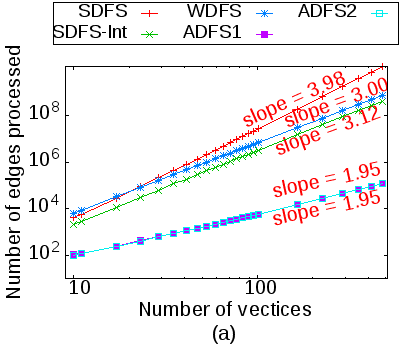
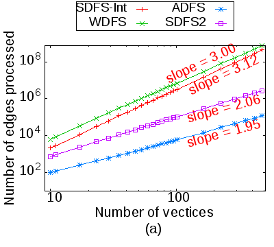
We first compare the total number of edges processed by the existing algorithms for insertion of $m={n\choose 2}$ edges, as a function of number of vertices in Figure 1 (a). Since the total number of edges is presented in logarithmic scale, the slope $x$ of a line depicts the growth of the total number of edges as $O(n^{x})$. The performance of SDFS, SDFS-Int and WDFS resemble their asymptotic bounds described in Table 1. For small values of $n$, WDFS performs worse than SDFS and SDFS-Int because of large difference between the constant terms in their asymptotic bounds, which is evident from their y-intercepts. However, the effect of constant term diminishes as the value of $n$ is increased. The most surprising aspect of this experiment is the exceptional performance of ADFS1 and ADFS2. Both ADFS1 and ADFS2 perform extremely faster than the other algorithms. Furthermore, ADFS1 and ADFS2 perform equally well despite the difference in their asymptotic complexity (see Table 1).

Inference $I_{1}$:  ADFS1 and ADFS2 perform equally well and much faster than other algorithms.

Remark: Inference $I_{1}$ is surprising because the complexity of ADFS1 and ADFS2 has been shown [6] to be $O(n^{3/2}\sqrt{m})$ and $O(n^{2})$ respectively. Moreover, we present a sequence of $m$ edge insertions where ADFS1 takes $\Omega(n^{3/2}\sqrt{m})$ time in Appendix B, proving the tightness of its analysis. Further, ADFS2 takes slightly more time than ADFS1, in order to maintain the data structure $\cal D$ (see Figure 11).

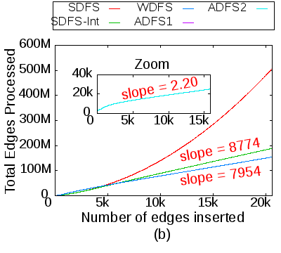
We now compare the total number of edges processed by the existing algorithms as a function of number of inserted edges in Figure 1 (b). The slopes of SDFS-Int, WDFS and ADFS represent the number of edges processed per edge insertion. Here again, the performance of SDFS, SDFS-Int and WDFS resembles with their worst case values (see Table 1). Similarly, both ADFS1 and ADFS2 perform equally well as noted in the previous experiment. When the graph is sparse ($m<<n\log^{3}n$), WDFS performs worse than SDFS because of high cost of update per edge insertion (see Table 1). Further, as expected the plots of SDFS-Int and WDFS grow linearly in $m$. This is because their update time per insertion is independent of $m$. However, the plots of ADFS1 and ADFS2 are surprising once again, because they become almost linear as the graph becomes denser. In fact, once the graph is no longer sparse, each of them processes $\approx 2$ edges per edge insertion to maintain the DFS tree. This improvement in the efficiency of ADFS1 and ADFS2 for increasing value of $m$ is counter-intuitive since more edges may be processed to rebuild the DFS tree as the graph becomes denser.

Inference $I_{2}$:  ADFS1/ADFS2 processes $\approx 2$ edges per insertion after the insertion of $O(n)$ edges.

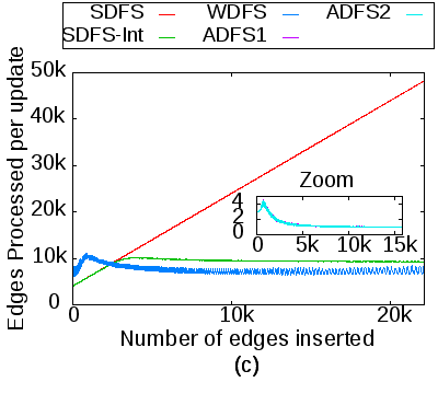
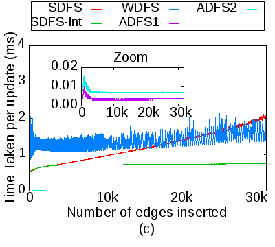
Finally, to investigate the exceptional behavior of ADFS1 and ADFS2, we compare the number of edges processed per edge insertion by the existing algorithms as a function of number of inserted edges in Figure 1 (c). Again, the expected behavior of SDFS, SDFS-Int and WDFS matches with their worst case bounds described in Table 1. The plot of WDFS shows the saw like structure owing to overlapped periodic rebuilding of the data structure used by the algorithm (see Section 3). Finally, the most surprising result of the experiment is the plot of ADFS1 and ADFS2 shown in the zoomed component of the plot. The number of edges processed per edge insertion sharply increases to roughly $5$ (for $n=1000$) when $m$ reaches $O(n)$ followed by a sudden fall to reach $1$ asymptotically. Note that the inserted edge is also counted among the processed edges, hence essentially the number of edges processed to update the DFS tree asymptotically reaches zero as the graph becomes dense. This particular behavior is responsible for the exceptional performance of ADFS1 and ADFS2.

Inference $I_{3}$:  Number of edges processed by ADFS1/ADFS2 for updating the DFS tree asymptotically reaches zero as the graph becomes denser.

To understand the exceptional behavior of ADFS1 and ADFS2 for random graphs inferred in $I_{1}$, $I_{2}$ and $I_{3}$, we investigate the structure of a DFS tree for random graphs in the following section.

5 Structure of a DFS tree: The broomstick

We know that SDFS, SDFS-Int and WDFS invariably rebuild the entire DFS tree on insertion of every edge. We thus state the first property of ADFS that differentiates it from other existing algorithms.

Property $P_{1}$:  ADFS rebuilds the DFS tree only on insertion of a cross edge.

Figure 2: The variation of (a) $p_{c}:$ Probability of next inserted edge being a cross edge, and (b) $l_{s}:$ Length of broomstick, with graph density. Different lines denote different number of vertices, starting at different points.

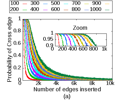
Let $T$ be any DFS tree of the random graph $G(n,m)$. Let $p_{c}$ denote the probability that the next randomly inserted edge is a cross edge in $T$. We first perform an experimental study to determine the behavior of $p_{c}$ as the number of edges in the graph increases. Figure 2 (a) shows this variation of $p_{c}$ for different values of $n$. The value $p_{c}$ starts decreasing sharply once the graph has $\Theta(n)$ edges. Eventually, $p_{c}$ asymptotically approaches $0$ as the graph becomes denser. Surely ADFS crucially exploits this behavior of $p_{c}$ in random graphs (using Property $P_{1}$). In order to understand the reason behind this behavior of $p_{c}$, we study the structure of a DFS tree of a random graph.

Broomstick Structure

The structure of a DFS tree can be described as that of a broomstick as follows. From the root of the DFS tree there exists a downward path on which there is no branching, i.e., every vertex has exactly one child. We refer to this path as the stick of the broomstick structure. The remaining part of the DFS tree (except the stick) is called the bristles of the broomstick.

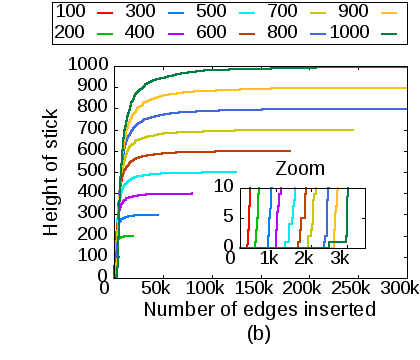
Let $l_{s}$ denote the length of the stick in the broomstick structure of the DFS tree. We now study the variation of $l_{s}$ as the edges are inserted in the graph. Figure 2 (b) shows this variation of $l_{s}$ for different values of $n$. Notice that the stick appears after the insertion of roughly $n\log n$ edges (see the zoomed part of Figure 2 (b)). After that $l_{s}$ increases rapidly to reach almost $90\%$ of its height within just $\approx 3n\log n$ edges, followed by a slow growth asymptotically approaching its maximum height only near $O(n^{2})$ edges. Since any newly inserted edge with at least one endpoint on the stick necessarily becomes a back edge, the sharp decrease in $p_{c}$ can be attributed to the sharp increase in $l_{s}$. We now theoretically study the reason behind the behavior of $l_{s}$ using properties of random graphs, proving explicit bounds for $l_{s}$ described in Theorem 1.1.

5.1 Length of the stick

The appearance of broomstick after insertion of $n\log n$ edges as shown in Figure 2 (b) can be explained by the connectivity threshold for random graphs (refer to Theorem 2.1). Until the graph becomes connected (till $\Theta(n\log n)$ edges), each component hangs as a separate subtree from the pseudo root $s$, limiting the value of $l_{s}$ to $0$. To analyze the length of $l_{s}$ for $m=\Omega(n\log n)$ edges, we first prove a succinct bound on the probability of existence of a long path without branching during a DFS traversal in $G(n,p)$ in the following lemma.

Lemma 5.1.

Given a random graph $G(n,p)$ with $p=(\log n_{0}+c)/n_{0}$, for any integer $n_{0}\leq n$ and $c\geq 1$, there exists a path without branching of length at least $n-n_{0}$ in the DFS tree of $G$ with probability at least $1-2/e^{c}$.

Proof.

Consider any arbitrary vertex $u=x_{1}$, the DFS traversal starting from $x_{1}$ continues along a path without branching so long as the currently visited vertex has at least one unvisited neighbor. Let $x_{j}$ denotes the $j^{th}$ vertex visited during the DFS on $G(n,p)$ starting from $x_{1}$. The probability that $x_{j}$ has at least one neighbor in the unvisited graph is $1-(1-p)^{n-j}$. We shall now calculate the probability that $\langle x_{1},\ldots,x_{n-n_{0}}\rangle$ is indeed a path. 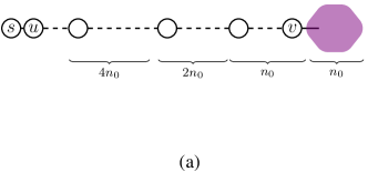Let $v=x_{n-n_{0}}$. We partition this sequence from $v$ towards $u$ into contiguous subsequences such that the first subsequence has length $n_{0}$ and $(i+1)^{th}$ subsequence has length $2^{i}n_{0}$ (see Figure 3 (a)). The probability of occurrence of a path corresponding to the $i^{th}$ subsequence is at least

$\left(1-\left(1-\frac{\log n_{0}+c}{n_{0}}\right)^{2^{i}n_{0}}\right)^{2^{i}n_{0}}\geq\left(1-\left(\frac{1}{n_{0}e^{c}}\right)^{2^{i}}\right)^{2^{i}n_{0}}\geq 1-\left(\frac{1}{e^{c}}\right)^{2^{i}}$

Hence, the probability that DFS from $u$ traverses a path of length $n-n_{0}$ is at least $\Pi_{i=0}^{\log_{2}n}\left(1-\frac{1}{t^{2^{i}}}\right)$ for $t=e^{c}$. The value of this expression is lower bounded by $1-\frac{2}{e^{c}}$ using the inequality
$\Pi_{i=0}^{i=\log_{2}t}\left(1-\frac{1}{t^{2^{i}}}\right)>1-\frac{2}{t}$, that holds for every $c\geq 1$ since it implies $t>2$. ∎

In order to establish a tight bound on the length of stick, we need to choose the smallest value of $n_{0}$ such that once we have a DFS path of length $n-n_{0}$ without branching, the subgraph induced by the remaining $n_{0}$ vertices is still connected. If the number of edges in this subgraph is $m_{0}$, according to Theorem 2.1, $n_{0}$ has to satisfy the following inequality.

$m_{0}=\frac{n_{0}^{2}}{n^{2}}m\geq\frac{n_{0}}{2}(\log n_{0}+c)$

It follows from Theorem 2.1 that the subgraph on $n_{0}$ vertices will be connected with probability at least $e^{-e^{-c}}\geq 1-e^{-c}$. Combining this observation with Lemma 5.1 and Theorem 2.2, it follows that the probability that DFS tree of $G(n,m)$ is a broomstick with stick length $\geq n-n_{0}$ is at least $1-\frac{c_{1}}{e^{c}}$ (for a small constant $c_{1}$). This probability tends to 1 for any increasing function $c(n)$, where $c(n)\geq 1$ for all $n$. We would like to state the following corollary that will be used later on.

Corollary 5.1.

For any random graph $G(n,m)$ with $m=2^{i}n\log n$, its DFS tree will have bristles of size at most $n/2^{i}$ with probability $1-O(1/n)$.

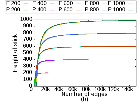
To demonstrate the tightness of our analysis we compare the length of the stick as predicted theoretically (for $c=1$) with the length determined experimentally in Figure 3 (b), which is shown to match exactly. This phenomenon emphasizes the accuracy and tightness of our analysis.

Figure 3: Estimating the length of ’stick’ in the DFS tree. (a) Partitioning the stick. (b) Comparison of experimentally evaluated (E) and theoretically predicted (P) value of length of the stick in the broomstick structure for different number of vertices.

6 Implications of broomstick property

Though the broomstick structure of DFS tree was earlier studied by Sibeyn [48], the crucial difference in defining the ‘stick’ to be without branches proved to be extremely significant. To emphasize its significance we now present a few applications of the broomstick structure of DFS tree, in particular Corollary 5.1 to state some interesting results. Note that the absence of branches on the stick is extremely crucial for all of the following applications.

Lemma 6.1.

For a uniformly random sequence of edge insertions, the number of edge insertions with both endpoints in bristles of the DFS tree will be $O(n\log n)$

Proof.

We split the sequence of edge insertions into phases and analyze the expected number of edges inserted in bristles in each phase. In the beginning of first phase there are $n\log n$ edges. In the $i^{th}$ phase, the number of edges in the graph grow from $2^{i-1}n\log n$ to $2^{i}n\log n$. It follows from Corollary 5.1 that $n_{i}$, the size of bristles in the $i^{th}$ phase will be at most $n/2^{i-1}$ with probability $1-O(1/n)$. Notice that each edge inserted during $i^{th}$ phase will choose its endpoints randomly uniformly. Therefore, the expected number of edges with both endpoints in bristles during the $i$th phase would be

$$m_{i}=\frac{n_{i}^{2}}{n^{2}}m\leq 2^{i}n\log n/2^{2(i-1)}=n\log n/2^{i-2}$$

Hence, the expected number of edges inserted with both endpoints in bristles is $\sum_{i=1}^{\log n}m_{i}=O(n\log n)$. ∎

In order to rebuild the DFS tree after insertion of a cross edge, it is sufficient to rebuild only the bristles of the broomstick, leaving the stick intact (as cross edges cannot be incident on it). Corollary 5.1 describes that the size of bristles decreases rapidly as the graph becomes denser making it easier to update the DFS tree. This crucial insight is not exploited by the algorithm SDFS, SDFS-Int or WDFS. We now state the property of ADFS that exploits this insight implicitly.

Property $P_{2}$:  ADFS modifies only the bristles of the DFS tree keeping the stick intact.

We define an incremental algorithm for maintaining a DFS for random graph to be bristle oriented if executing the algorithm $\cal A$ on $G$ is equivalent to executing the algorithm on the subgraph induced by the bristles. Clearly, ADFS is bristle oriented owing to property $P_{2}$ and the fact that it processes only the edges with both endpoints in rerooted subtree (refer to Section 3). We now state an important result for any bristle oriented algorithm (and hence ADFS) as follows.

Lemma 6.2.

For any bristle oriented algorithm $\cal A$ if the expected total time taken to insert the first $2n\log n$ edges of a random graph is $O(n^{\alpha}\log^{\beta}n)$ (where $\alpha>0$ and $\beta\geq 0$), the expected total time taken to process any sequence of $m$ edge insertions is $O(m+n^{\alpha}\log^{\beta}n)$.

Proof.

Recall the phases of edge insertions described in the proof of Lemma 6.1, where in the $i^{th}$ phase the number of edges in the graph grow from $2^{i-1}n\log n$ to $2^{i}n\log n$. The size of bristles at the beginning of $i^{th}$ phase is $n_{i}=n/2^{i-1}$ w.h.p.. Further, note that the size of bristles is reduced to half during the first phase, and the same happens in each subsequent phase w.h.p. (see Corollary 5.1). Also, the expected number of edges added to subgraph represented by the bristles in $i^{th}$ phase is $O(n_{i}\log n_{i})$ (recall the proof of Lemma 6.1). Since $\cal A$ is bristle oriented, it will process only the subgraph induced by the bristles of size $n_{i}$ in the $i^{th}$ phase. Thus, if $\cal A$ takes $O(n^{\alpha}\log^{\beta}n)$ time in first phase, the time taken by $\cal A$ in the $i^{th}$ phase is $O(n_{i}^{\alpha}\log^{\beta}n_{i})$. The second term $O(m)$ comes from the fact that we would need to process each edge to check whether it lies on the stick. This can be easily done in $O(1)$ time by marking the vertices on the stick. The total time taken by $\cal A$ is $O(n^{\alpha}\log^{\beta}n)$ till the end of the first phase and in all subsequent phases is given by the following

$$=m+\sum_{i=2}^{\log n}cn_{i}^{\alpha}\log^{\beta}n_{i} \leq\sum_{i=2}^{\log n}c\Big{(}\frac{n}{2^{i-1}}\Big{)}^{\alpha}\log^{\beta}\Big{(}\frac{n}{2^{i-1}}\Big{)}$$

$$\leq m+cn^{\alpha}\log^{\beta}n\sum_{i=2}^{\log n}\frac{1}{2^{(i-1)\alpha}} (\text{for $\beta\geq 0$})$$

$$\leq m+c*c^{\prime}n^{\alpha}\log^{\beta}n (\sum_{i=2}^{\log n}\frac{1}{2^{(i-1)\alpha}}=c^{\prime},\text{for $\alpha>0$})$$

Thus, the total time taken by $\cal A$ is $O(m+n^{\alpha}\log^{\beta}n)$. ∎

Lemma 6.1 and Lemma 6.2 immediately implies the similarity of ADFS1 and ADFS2 as follows.

Equivalence of ADFS1 and ADFS2

On insertion of a cross edge, ADFS performs a path reversal and collects the back edges that are now converted to cross edges, to be iteratively inserted back into the graph. ADFS2 differs from ADFS1 only by imposing a restriction on the order in which these collected edges are processed. However, for sparse graphs ($m=O(n)$) this restriction does not change its worst case performance (see Table 1). Now, Lemma 6.2 states that the time taken by ADFS to incrementally process any number of edges is of the order of the time taken to process a sparse graph (with only $2n\log n$ edges). Thus, ADFS1 performs similar to ADFS2 even for dense graphs. Particularly, the time taken by ADFS1 for insertion of any $m\leq{n\choose 2}$ edges is $O(n^{2}\sqrt{\log n})$, i.e., $O(n^{3/2}m_{0}^{1/2})$ for $m_{0}=2n\log n$. Thus, we have the following theorem.

Theorem 6.1.

Given a uniformly random sequence of arbitrary length, the expected time complexity of ADFS1 for maintaining a DFS tree incrementally is $O(n^{2}\sqrt{\log n})$.

Remark: The factor of $O(\sqrt{\log n})$ in the bounds of ADFS1 and ADFS2 comes from the limitations of our analysis whereas empirically their performance matches exactly.

7 New algorithms for Random Graphs

Inspired by Lemma 6.1 and Lemma 6.2 we propose the following new algorithms.

Simple variant of SDFS (SDFS2) for random undirected graphs

We propose a bristle oriented variant of SDFS which satisfies the properties $P_{1}$ and $P_{2}$ of ADFS, i.e., it rebuilds only the bristles of the DFS tree on insertion of only cross edges. This can be done by marking the vertices in the bristles as unvisited and performing the DFS traversal from the root of the bristles. Moreover, we also remove the non-tree edges incident on the stick of the DFS tree. As a result, SDFS2 would process only the edges in the bristles, making it bristle oriented. Now, according to Lemma 6.2 the time taken by SDFS2 for insertion of $m=2n\log n$ edges (and hence any $m\leq{n\choose 2}$) is $O(m^{2})=O(n^{2}\log^{2}n)$. Thus, we have the following theorem.

Theorem 7.1.

Given a random graph $G(n,m)$, the expected time taken by SDFS2 for maintaining a DFS tree of $G$ incrementally is $O(n^{2}\log^{2}n)$.

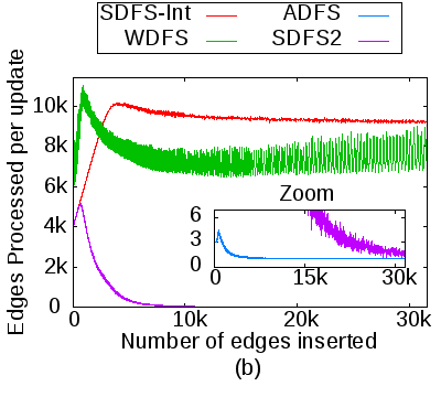
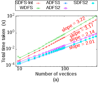
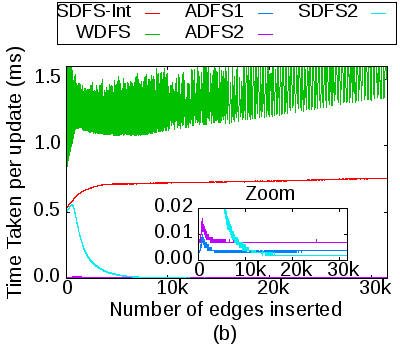
We now compare the performance of the proposed algorithm SDFS2 with the existing algorithms. Figure 4 (a) compares the total number of edges processed for insertion of $m={n\choose 2}$ edges, as a function of number of vertices in the logarithmic scale. As expected SDFS2 processes $\tilde{O}(n^{2})$ edges similar to ADFS. Figure 4 (b) compares the number of edges processed per edge insertion as a function of number of inserted edges. Again, as expected SDFS2 performs much better than WDFS and SDFS-Int, performing asymptotically equal to ADFS as the performance differs only when the graph is very sparse ($\approx n\log n$). Interestingly, despite the huge difference in number of edges processed by SDFS2 with respect to ADFS (see Figure 4 (a)), it is faster than ADFS2 and equivalent to ADFS1 in practice (see Figure 12 (a)).

Figure 4: Comparison of existing and proposed algorithms on undirected graphs: (a) Total number of edges processed for insertion of $m={n\choose 2}$ edges for different values of $n$ in logarithmic scale (b) Number of edges processed per edge insertion for $n=1000$ and up to $n\sqrt{n}$ edge insertions. See Figure 12 for corresponding time plot.

Experiments on directed graphs and directed acyclic graphs

The proposed algorithm SDFS2 also works for directed graphs. It is easy to show that Corollary 5.1 also holds for directed graphs (with different constants). Thus, the properties of broomstick structure and hence the analysis of SDFS2 can also be proved for directed graphs using similar arguments. The significance of this algorithm is highlighted by the fact that there does not exists any algorithm for maintenance of incremental DFS for general directed graphs requiring $o(m^{2})$ time. Moreover, FDFS also performs very well and satisfies the properties $P_{1}$ and $P_{2}$ (similar to ADFS in undirected graphs). Note that extension of FDFS for directed graphs is not known to have complexity any better than $O(m^{2})$, yet for random directed graphs we can prove it to be $\tilde{O}(n^{2})$ using Lemma 6.2.

Figure 5: Comparison of existing and proposed algorithms on directed graphs: (a) Total number of edges processed for insertion of $m={n\choose 2}$ edges for different values of $n$ in logarithmic scale (b) Number of edges processed per edge insertion for $n=1000$ and up to $n\sqrt{n}$ edge insertions. See Figure 13 for corresponding time plot.

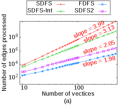
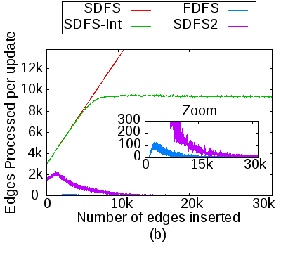
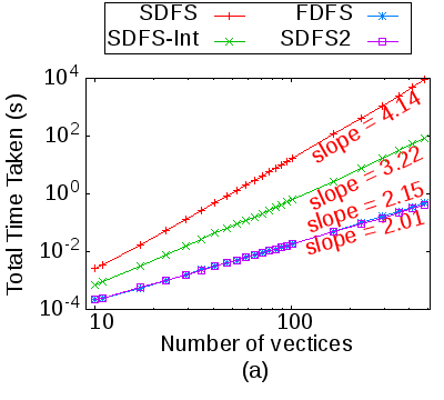
We now compare the performance of the proposed algorithm SDFS2 with the existing algorithms in the directed graphs. Figure 5 (a) compares the total number of edges processed for insertion of $m={n\choose 2}$ edges, as a function of number of vertices in the logarithmic scale. As expected SDFS2 processes $\tilde{O}(n^{2})$ edges similar to FDFS. Figure 5 (b) compares the number of edges processed per edge insertion as a function of number of inserted edges for directed graphs. Thus, the proposed SDFS2 performs much better than SDFS, and asymptotically equal to FDFS. Again despite the huge difference in number of edges processed by SDFS2 with respect to FDFS, it is equivalent to FDFS in practice (see Figure 5 (a) and Figure 13 (a)).

Figure 6: Comparison of existing and proposed algorithms on DAGs: (a) Total number of edges processed for insertion of $m={n\choose 2}$ edges for different values of $n$ in logarithmic scale (b) Number of edges processed per edge insertion for $n=1000$ and up to $n\sqrt{n}$ edge insertions. See Figure 14 for corresponding time plots. (c) Comparison of variation of length of broomstick for 1000 vertices and different values of $m$. Different lines denote the variation for different type of graphs. Zoomed portion shows the start of each line.

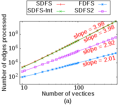
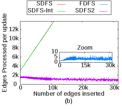
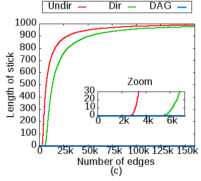
Finally, we compare the performance of the proposed algorithm SDFS2 with the existing algorithms in DAGs. Figure 6 (a) compares the total number of edges processed for insertion of $m={n\choose 2}$ edges, as a function of number of vertices in the logarithmic scale. Both SDFS and SDFS-Int perform equally which was not the case when the experiment was performed on undirected (Figure 1) or directed graphs (Figure 5). Moreover, SDFS2 processes around $\tilde{O}(n^{3})$ edges which is more than the proven bound of $\tilde{O}(n^{2})$ for undirected and directed graphs. However, FDFS processes $\tilde{O}(n^{2})$ edges as expected. Figure 6 (b) compares the number of edges processed per edge insertion as a function of number of inserted edges. Again, both SDFS and SDFS-Int perform similarly and SDFS2 does not perform asymptotically equal to FDFS even for dense graphs. Notice that the number of edges processed by SDFS2 does not reach a peak and then asymptotically move to zero as in case of undirected and general directed graphs. Also, FDFS performs much better (similar to ADFS for undirected graphs) for DAGs as compared to directed graphs. Again, despite superior performance on random DAGs, for general DAGs it can be shown that the analysis of FDFS is indeed tight (see Appendix C).

To understand the reason behind this poor performance of SDFS-Int and SDFS2 on DAGs, we compare the variation in length of broomstick for the undirected graphs, general directed graphs and DAGs in Figure 6 (c). The length of the broomstick varies as expected for undirected and general directed graphs but always remains zero for DAGs. This is because the stick will appear only if the first neighbor of the pseudo root $s$ visited by the algorithm is the first vertex (say $v_{1}$) in the topological ordering of the graph. Otherwise $v_{1}$ hangs as a separate child of $s$ because it not reachable from any other vertex in the graph. Since the edges in $G(n,m)$ model are permuted randomly, with high probability $v_{1}$ may not be the first vertex to get connected to $s$. The same argument can be used to prove branchings at every vertex on the stick. Hence, with high probability there would be some bristles even on the pseudo root $s$. This explains why SDFS-Int performs equal to SDFS as it works same as SDFS until all the vertices are visited. SDFS2 only benefits from the inserted edges being reverse cross edges which are valid in a DFS tree and hence avoids rebuilding on every edge insertion. Thus, Corollary 5.1 and hence the bounds for SDFS2 proved in Theorem 7.1 are not valid for the case of DAGs as resulting in performance described above. Moreover, the absence of the broomstick phenomenon can also be proved for other models of random graphs for DAGs [12] using the same arguments.

Finally, Lemma 6.1 also inspires the following interesting applications of SDFS2 in the semi-streaming environment as follows.

Semi-streaming algorithms

In the streaming model we have two additional constraints. Firstly, the input data can be accessed only sequentially in the form of a stream. The algorithm can do multiple passes on the stream, but cannot access the entire stream. Secondly, the working memory is considerably smaller than the size of the entire input stream. For graph algorithms, a semi-streaming model allows the size of the working memory to be $\tilde{O}(n)$.

The DFS tree can be trivially computed using $O(n)$ passes over the input graph in the semi-streaming environment, each pass adding one vertex to the DFS tree. However, computing the DFS tree in even $\tilde{O}(1)$ passes is considered hard [17]. To the best of our knowledge, it remains an open problem to compute the DFS tree using even $o(n)$ passes in any relaxed streaming environment [42, 46]. Now, some of the direct applications of a DFS tree in undirected graphs are answering connectivity, bi-connectivity and 2-edge connectivity queries. All these problems are addressed efficiently in the semi-streaming environment using a single pass by the classical work of Westbrook and Tarjan [53]. On the other hand, for the applications of a DFS tree in directed graphs as strong connectivity, strong lower bounds of space for single-pass semi-streaming algorithms have been shown . Borradaile et al. [8] showed that any algorithm requires a a working memory of $\Omega(\epsilon m)$ to answer queries of strong connectivity, acyclicity or reachability from a vertex require with probability greater than $(1+\epsilon)/2$.

We now propose a semi-streaming algorithm for maintaining Incremental DFS for random graphs. The key idea to limit the storage space required by this algorithm is to just discard those edges from the stream whose at least one endpoint is on the stick of the DFS tree. As described earlier, this part of DFS tree corresponding to the stick will never be modified by the insertion of any edge. If both the endpoints of the edge lie in bristles, we update the DFS tree using ADFS/SDFS2. Lemma 6.1 implies that the expected number of edges stored will be $O(n\log n)$. In case we use SDFS2 (for directed graphs) we also delete the non-tree edges incident on the stick. Hence, we have the following theorem.

Theorem 7.2.

Given a random graph $G(n,m)$, there exists a single pass semi-streaming algorithm for maintaining the DFS tree incrementally, that requires $O(n\log n)$ space.

Further, for random graphs even strong connectivity can be solved using a single pass in the streaming environment by SDFS2 as follows. Now, SDFS2 keeps only the tree edges and the edges in the bristles. For answering strong connectivity queries, we additionally store the highest edge from each vertex on the stick. The strongly connected components can thus be found by a single traversal on the DFS tree [49]. Thus, our semi-streaming algorithm SDFS2 not only gives a solution for strong connectivity in the streaming setting but also establishes the difference in its hardness for general graphs and random graphs. To the best of our knowledge no such result was known for any graph problem in streaming environment prior to our work. Thus, we have the following theorem.

Theorem 7.3.

Given a random graph $G(n,m)$, there exists a single pass semi-streaming algorithm for maintaining a data structure that answers strong connectivity queries in $G$ incrementally, requiring $O(n\log n)$ space.

8 Incremental DFS on real graphs

We now evaluate the performance of existing and proposed algorithms on real graphs. Recall that for random graphs, bristles represent the entire DFS tree until the insertion of $\Theta(n\log n)$ edges. This forces SDFS2 to rebuild the whole tree requiring total $\Omega(n^{2})$ time even for sparse random graphs, whereas ADFS and FDFS only partially rebuild the DFS tree and turn out to be much better for sparse random graphs (see Figure 4 (b), 5 (b) and 6 (b)). Now, most graphs that exist in real world are known to be sparse [36]. Here again, both ADFS and FDFS perform much better as compared to SDFS2 and other existing algorithms. Thus, we propose another simple variant of SDFS (SDFS3), which is both easy to implement and performs very well even on real graphs (much better than SDFS2).

8.1 Proposed algorithms for real graphs (SDFS3)

The primary reason behind the superior performance of ADFS and FDFS is the partial rebuilding of the DFS tree upon insertion of an edge. However, the partial rebuilding by SDFS2 is significant only when the broomstick has an appreciable size, which does not happen until the very end in most of the real graphs. With this insight, we propose new algorithms for directed and undirected graphs. The aim is to rebuild only that region of the DFS tree which is affected by the edge insertion.

• Undirected Graphs
  On insertion of a cross edge $(x,y)$, ADFS rebuilds one of the two candidate subtrees hanging from $LCA(x,y)$ containing $x$ or $y$. We propose algorithm SDFS3 that will rebuild only the smaller subtree (less number of vertices) among the two candidate subtrees (say $x\in T_{1}$ and $y\in T_{2}$). This heuristic is found to be extremely efficient compared to rebuilding one of $T_{1}$ or $T_{2}$ arbitrarily. The smaller subtree, say $T_{2}$, can be identified efficiently by simultaneous traversal in both $T_{1}$ and $T_{2}$. and terminate as soon as either one is completely traversed. This takes time of the order of $|T_{2}|$. We then mark the vertices of $T_{2}$ as unvisited and start the traversal from $y$ in $T_{2}$, hanging the newly created subtree from edge $(x,y)$.

• Directed Graphs
  On insertion of an anti-cross edge $(x,y)$, FDFS rebuilds the vertices reachable from $y$ in the subgraph induced by a candidate set of subtrees described in Section 3. FDFS identifies this affected subgraph using the DFN number of the vertices. Thus, this DFN number also needs to be updated separately after rebuilding the DFS tree. This is done by building an additional data structure while the traversal is performed, which aids in updating the DFN numbers efficiently. We propose SDFS3 to simply mark all the subtrees in this candidate set as unvisited and proceed the traversal from $(x,y)$. The traversal then continues from each unvisited root of the subtrees marked earlier, implicitly restoring the DFN number of each vertex.

8.2 Experimental Setup

The algorithms are implemented in C++ using STL (standard template library), and built with GNU g++ compiler (version 4.4.7) with optimization flag $-O3$. The correctness of our code was exhaustively verified on random inputs by ensuring the absence of anti-cross edges (or cross edge) in directed (or undirected) graphs. Our experiments were run on Intel Xeon E5-2670V 2.5 GHz 2 CPU-IvyBridge (20-cores per node) on HP-Proliant-SL-230s-Gen8 servers with 1333 MHz DDR3 RAM of size 768 GB per node. Each experiment was performed using a single dedicated processor.

8.3 Datasets used for evaluation on Real Graphs

We consider the following types of graphs in our experiments:

• Internet topology: These datasets represent snapshots of network topology on CAIDA project (asCaida [32, 33]), Oregon Route Views Project’s Autonomous Systems (ass733 [32, 33]) and Internet autonomous systems (intTop [54, 29]).

• Collaboration networks: These datasets represent the collaboration networks as recorded on arxiv’s High-Energy-Physics groups of Phenomenology (arxvPh [31, 13, 29]) and Theory (arxvTh [31, 13, 29]), and on DBLP (dblp [34, 13, 29]).

• Online communication: These datasets represent communication of linux kernel messages (lnKMsg [29]), Gnutella peer-to-peer file sharing network (gnutella [45, 33]), Slashdot’s message exchange (slashDt [20, 29]), Facebook’s wall posts (fbWall [52, 29]), Democratic National Committee’s (DNC) email correspondence (dncCoR [29]), Enron email exchange (enron [28, 29]), Digg’s reply correspondence (digg [11, 29]) and UC Irvine message exchange (ucIrv [43, 29])

• Friendship networks: These datasets represent the friendship networks of Flickr (flickr [40, 29], Digg (diggNw [22, 29]), Epinion (epinion [35, 29]), Facebook (fbFrnd [52, 29]) and Youtube (youTb [39, 29]).

• Other interactions: These datasets represent the other networks as Chess game interactions (chess [29]), user loans on Prosper (perLoan [29]), hyperlink network of Wikipedia (wikiHy [39, 29]), voting in elections on Wikipedia (wikiEl [30, 29]) and conflict resolution on Wikipedia (wikiC [9, 29]).

In some of these datasets there are some rare instances in which edges are deleted (not present in new snapshot). Thus, in order to use these datasets for evaluation of incremental algorithms we ignore the deletion of these edges (and hence reinsertion of deleted edges). Moreover, in several datasets the edges are inserted in form of batches (having same insertion time), where the number of batches are significantly lesser than the number of inserted edges. Almost all the algorithms (except FDFS and SDFS3) can be tweaked to handle such batch insertions more efficiently, updating the DFS tree once after insertion of an entire batch, instead of treating every edge insertion individually.

Dataset	$n$	$m|m^{*}$	$\frac{m}{n}|\frac{m}{m^{*}}$	ADFS1	ADFS2	SDFS3	SDFS2	SDFS	WDFS
ass733	7.72K	21.47K	2.78	1.00	1.88	34.12	639.50	1.13K	2.99K
		721.00	29.77	1.00	2.71	38.43	35.57	54.14	95.43
intTop	34.76K	107.72K	3.10	1.00	2.14	111.32	3.78K	8.15K	14.65K
		18.27K	5.89	1.00	6.07	99.47	320.49	1.83K	2.24K
fbFrnd	63.73K	817.03K	12.82	1.00	2.18	146.58	2.02K	14.67K	11.75K
		333.92K	2.45	1.00	8.10	141.07	491.24	7.63K	4.27K
wikiC	116.84K	2.03M	17.36	1.00	1.82	249.45	3.09K	$>$22.56K	$>$22.56K
		205.59K	9.86	1.00	2.26	246.49	2.69K	4.39K	3.35K
arxvTh	22.91K	2.44M	106.72	1.00	1.81	28.31	3.41K	$>$39.96K	9.72K
		210.00	11.64K	1.00	6.74	32.01	8.63	13.24	2.84K
arxvPh	28.09K	3.15M	112.07	1.00	2.38	57.94	2.54K	$>$36.29K	11.32K
		2.26K	1.39K	1.00	8.25	70.75	103.23	192.22	3.17K
dblp	1.28M	3.32M	2.59	1.00	1.60	$>$22.07K	$>$22.07K	$>$22.07K	$>$22.07K
		1.72M	1.93	1.00	1.84	$>$21.26K	$>$21.26K	$>$21.26K	$>$21.26K
youTb	3.22M	9.38M	2.91	1.00	3.53	$>$347.00	$>$347.00	$>$347.00	$>$347.00
		203.00	46.18K	1.26	2.26	$>$322.18	1.00	1.00	260.73

Table 2: Comparison of time taken by different algorithms, relative to the fastest (shown in bold), for maintaining incremental DFS on real undirected graphs. See Table 4 for corresponding table comparing the exact performance of different algorithms.

Dataset	$n$	$m|m^{*}$	$\frac{m}{n}|\frac{m}{m^{*}}$	FDFS	SDFS3	SDFS2	SDFS
dncCoR	1.89K	5.52K	2.92	1.55	1.00	2.27	9.86
		4.01K	1.38	1.55	1.00	2.00	7.18
ucIrv	1.90K	20.30K	10.69	1.69	1.00	2.25	21.81
		20.12K	1.01	1.78	1.00	2.35	22.14
chess	7.30K	60.05K	8.22	1.94	1.00	2.54	20.00
		100.00	600.46	52.04	26.14	1.00	1.00
diggNw	30.40K	85.25K	2.80	1.00	1.33	3.60	14.50
		81.77K	1.04	1.00	1.38	3.78	11.96
asCaida	31.30K	97.84K	3.13	1.00	4.31	13.60	64.71
		122.00	801.98	12.57	42.62	1.01	1.00
wikiEl	7.12K	103.62K	14.55	1.01	1.00	2.58	51.80
		97.98K	1.06	1.00	1.00	2.53	52.38
slashDt	51.08K	130.37K	2.55	1.03	1.00	2.78	5.85
		84.33K	1.55	1.04	1.00	2.07	3.79
lnKMsg	27.93K	237.13K	8.49	1.82	1.00	2.40	23.24
		217.99K	1.09	1.77	1.00	2.30	23.13
fbWall	46.95K	264.00K	5.62	1.29	1.00	2.49	14.84
		263.12K	1.00	1.31	1.00	2.73	17.11
enron	87.27K	320.15K	3.67	1.00	1.55	5.66	67.58
		73.87K	4.33	1.00	1.48	2.61	14.00
gnutella	62.59K	501.75K	8.02	1.23	1.00	2.54	19.13
		9.00	55.75K	1.17K	1.04K	1.03	1.00
epinion	131.83K	840.80K	6.38	1.32	1.00	2.29	17.77
		939.00	895.42	95.27	93.62	1.00	1.00
digg	279.63K	1.73M	6.19	1.00	1.18	3.96	$>$29.28
		1.64M	1.05	1.00	1.34	4.08	$>$30.92
perLoan	89.27K	3.33M	37.31	1.00	7.10	30.70	$>$639.03
		1.26K	2.65K	2.13	13.18	1.00	1.01
flickr	2.30M	33.14M	14.39	-	-	-	-
		134.00	247.31K	$>$476.50	$>$476.50	1.01	1.00
wikiHy	1.87M	39.95M	21.36	-	-	-	-
		2.20K	18.18K	$>$69.26	$>$69.26	1.00	1.13

Table 3: Comparison of time taken by different algorithms, relative to the fastest (shown in bold), for maintaining incremental DFS on real directed graphs. If all algorithms exceed 100hrs giving no fastest algorithm, their corresponding relative time is not shown (-). See Table 5 for corresponding table comparing the exact performance of different algorithms.

8.4 Evaluation

The comparison of the performance of the existing and the proposed algorithms for real undirected graphs and real directed graphs is shown in Table 2 and Table 3 respectively. To highlight the relative performance of different algorithms, we present the time taken by them relative to that of the fastest algorithm (see Appendix F for the exact time and memory used by different algorithms). In case the time exceeded $100$hrs the process was terminated, and we show the relative time in the table with a ’$>$’ sign and the ratio corresponding to $100$hrs. For each dataset, the first row corresponds to the experiments in which the inserted edges are processed one by one, and the second row corresponds to the experiments in which the inserted edges are processed in batches ($m^{*}$ denotes the corresponding number of batches). The density of a graph can be judged by comparing the average degree ($m/n$) with the number of vertices ($n$). Similarly, the batch density of a graph can be judged by comparing the average size of a batch ($m/m^{*}$) with the number of vertices ($n$).

For undirected graphs, Table 2 clearly shows that ADFS1 outperforms all the other algorithms irrespective of whether the edges are processed one by one or in batches (except youTb). Moreover, despite ADFS2 having better worst case bounds than ADFS1, the overhead of maintaining its data structure $\cal D$ leads to inferior performance as compared to ADFS1. Also, SDFS2 significantly improves over SDFS ($>2$ times). However, by adding a simple heuristic, SDFS3 improves over SDFS2 by a huge margin ($>10$ times) which becomes even more significant when the graph is very dense (arxvT and arxvPh). Also, note that even SDFS3 performs a lot worse than ADFS ($>30$ times) despite having a profound improvement over SDFS2. Further, despite having good worst case bounds, WDFS seems to be only of theoretical interest and performs worse than even SDFS in general. However, if the graph is significantly dense (fbFrnd, wikiC, arxvT and arxvPh), WDFS performs better than SDFS but still far worse than SDFS2. Now, in case of batch updates, SDFS3 is the only algorithm that is unable to exploit the insertion of edges in batches. Hence, SDFS3 performs worse than SDFS2 and even SDFS if the batch density is significantly high (arxvTh and youTb). Finally, if the batch density is extremely high (youTb), the simplicity of SDFS and SDFS2 results in a much better performance than even ADFS.

Observations: For real undirected graphs • ADFS outperforms all other algorithms by a huge margin, with ADFS1 always performing mildly better than ADFS2. • SDFS2 mildly improves SDFS, whereas SDFS3 significantly improves SDFS2. • WDFS performs even worse than SDFS for sparse graphs.

For directed graphs, Table 3 shows that both FDFS and SDFS3 perform almost equally well (except perLoan) and outperform all other algorithms when the edges are processed one by one. In general SDFS3 outperforms FDFS marginally when the graph is dense (except slashDt and perLoan). The significance of SDFS3 is further highlighted by the fact that it is much simpler to implement as compared to FDFS. Again, SDFS2 significantly improves over SDFS ($>2$ times). Further, by adding a simple heuristic, SDFS3 improves over SDFS2 ($>2$ times), and this improvement becomes more pronounced when the graph is very dense (perLoan). Now, in case of batch updates, both FDFS and SDFS3 are unable to exploit the insertion of edges in batches. Hence, they perform worse than SDFS and SDFS2 for batch updates, if the average size of a batch is at least $600$. SDFS and SDFS2 perform almost equally well in such cases with SDFS performing marginally better than SDFS2 when the batch density is significantly high (asCaida, gnutella and flickr).

Observations: For real directed graphs • FDFS and SDFS3 outperform all other algorithms unless batch density is high, where trivial SDFS is better. • SDFS3 performs better than FDFS in dense graphs. • SDFS2 mildly improves SDFS, and SDFS3 mildly improves SDFS2.

Overall, we propose the use of ADFS1 and SDFS3 for undirected and directed graphs respectively. Although SDFS3 performs very well on real graphs, its worst case time complexity is no better than that of SDFS on general graphs (see Appendix D). Finally, in case the batch density of the input graph is substantially high, we can simply use the trivial SDFS algorithm.

Remark: The improvement of SDFS3 over SDFS2 is substantially better on undirected graphs than on directed graphs. Even then ADFS1 outperforms SDFS3 by a huge margin. Also, when the batch density is extremely high (youTb), ADFS1 performs only mildly slower than the fastest algorithm (SDFS). These observations further highlight the significance of ADFS1 in practice.

9 Conclusions

Our experimental study of existing algorithms for incremental DFS on random graphs presented some interesting inferences. Upon further investigation, we discovered an important property of the structure of DFS tree in random graphs: the broomstick structure. We then theoretically proved the variation in length of the stick of the DFS tree as the graph density increases, which also exactly matched the experimental results. This led to several interesting applications, including the design of an extremely simple algorithm SDFS2. This algorithm theoretically matches and experimentally outperforms the state-of-the-art algorithm in dense random graphs. It can also be used as a single pass semi-streaming algorithm for incremental DFS as well as strong connectivity in random graphs, which also establishes the difference in hardness of strong connectivity in general graphs and random graphs. Finally, for real world graphs, which are usually sparse, we propose a new simple algorithm SDFS3 which performs much better than SDFS2. Despite being extremely simple, it almost always matches the performance of FDFS in directed graphs. However, for undirected graphs ADFS was found to outperform all algorithms (including SDFS3) by a huge margin motivating its use in practice.

For future research directions, recall that ADFS (see Inference $I_{2}$) performs extremely well even on sparse random graphs. Similarly, the performance of FDFS and SDFS3 is also very good even on sparse random graphs. However, none of these have asymptotic bounds any better than $\tilde{O}(n^{2})$. After preliminary investigation, we believe that the asymptotic bounds for ADFS and FDFS (in DAGs) should be $O(m+n\text{polylog}n)$ for random graphs. Also, we believe that the asymptotic bounds for SDFS3 and FDFS (in directed graphs) should be $O(m+n^{4/3}\text{polylog}n)$ for random graphs. It would be interesting to see if it is possible to prove these bounds theoretically.

Appendix A Performance analysis in terms of edges

Figure 7: Comparison of total time taken and time taken by LCA/LA data structure by the most efficient algorithms for insertion of $m={n\choose 2}$ edges for different values of $n$.

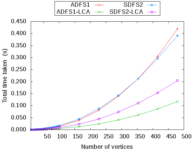
Most of the algorithms analyzed in this paper require dynamic maintenance of a data structure for answering LCA and LA (level ancestor) queries. The LCA/LA data structures used by Baswana and Khan [6] takes $O(1)$ amortized time to maintain the data structure for every vertex whose ancestor is changed in the DFS tree. However, it is quite difficult to implement and seems to be more of theoretical interest. Thus, we use a far simpler data structure whose maintenance require $O(\log n)$ time for every vertex whose ancestor is changed in the DFS tree. Figure 7 shows that the time taken by these data structures is insignificant in comparison to the total time taken by the algorithm. Analyzing the number of edges processed instead of time taken allows us to ignore the time taken for maintaining and querying this LCA/LA data structure. Moreover, the performance of ADFS and FDFS is directly proportional to the number of edges processed along with some vertex updates (updating DFN numbers for FDFS and LCA/LA structure for ADFS). However, the tasks related to vertex updates can be performed in $\tilde{O}(1)$ time using dynamic trees [51]. Thus, the actual performance of these algorithms is truly depicted by the number of edges processed, justifying our evaluation of relative performance of different algorithms by comparing the number of edges processed.

Appendix B Worst Case Input for ADFS1

Figure 8: Example to demonstrate the tightness of the ADFS1. (a) Beginning of a phase with vertex sets $A$, $B$ and $X$. (b) Phase begins with addition of two vertex sets $C$ and $D$. The first stage begins with the insertion of a back edge $(a_{1},b_{k+1})$ and a cross edge $(b_{1},c_{k})$. (c) The rerooted subtree with the edges in $A\times X$ and $(b_{k+1},a_{1})$ as cross edges. (d) Final DFS tree after the first stage. (e) Final DFS tree after first phase. (f) New vertex sets $A^{\prime}$, $B^{\prime}$ and $X$ for the next phase.

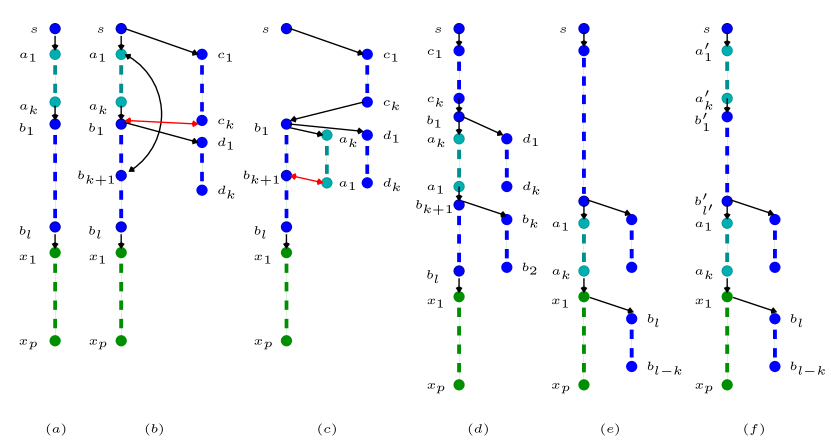
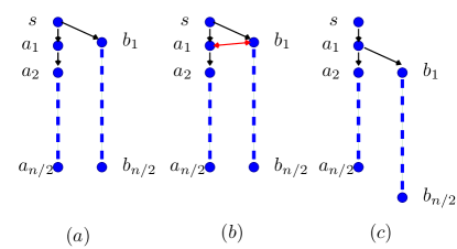
We now describe a sequence of $\Theta(m)$ edge insertions for which ADFS1 takes $\Theta(n^{3/2}m^{1/2})$ time. Consider a graph $G=(V,E)$ where the set of vertices $V$ is divided into two sets $V^{\prime}$ and $I$, each of size $\Theta(n)$. The vertices in $V^{\prime}$ are connected in the form of a chain (see Figure 8 (a)) and the vertices in $I$ are isolated vertices. Thus, it is sufficient to describe only the maintenance of DFS tree for the vertices in set $V^{\prime}$, as the vertices in $I$ will exist as isolated vertices connected to the dummy vertex $s$ in the DFS tree (recall that $s$ is the root of the DFS tree).

We divide the sequence of edge insertions into $n_{p}$ phases, where each phase is further divided into $n_{s}$ stages. At the beginning of each phase, we identify three vertex sets from the set $V^{\prime}$, namely $A=\{a_{1},...,a_{k}\}$, $B=\{b_{1},...,b_{l}\}$ and $X=\{x_{1},...,x_{p}\}$, where $k,l,p\leq n$ are integers whose values will be fixed later. The value of $l$ is $p$ in the first phase and decreases by $k$ in each subsequent phase. Figure 8 (a) shows the DFS tree of the initial graph. We add $p*k$ edges of the set $A\times X$ to the graph. Clearly, the DFS tree does not change since all the inserted edges are back edges. Further, we extract two sets of vertices $C=\{c_{1},...,c_{k}\}$ and $D=\{d_{1},...,d_{k}\}$ from $I$ and connect them in the form of a chain as shown in Figure 8 (b).

Now, the first stage of each phase starts with the addition of the back edge $(a_{1},b_{k+1})$ followed by the cross edge $(b_{1},c_{k})$. As a result ADFS1 will reroot the tree $T(a_{1})$ as shown in the Figure 8 (c) (extra $O(1)$ vertices from $I$ are added to $C$ to ensure the fall of $T(a_{1})$ instead of $T(c_{1})$). This rerooting makes $(b_{k+1},a_{1})$ a cross edge. Moreover, all $p*k$ edges of set $A\times X$ also become cross edges. ADFS1 will collect all these edges and process them in $\Omega(p*k)$ time. Since the algorithm can process these edges arbitrarily, it can choose to process $(b_{k+1},a_{1})$ first. It will result in the final DFS tree as shown in Figure 8 (d), converting all the cross edges in $A\times X$ to back edges and bringing an end to the first stage. Note the similarity between Figure 8 (b) and Figure 8 (d): the set $C$ is replaced by the set $D$, and the set $D$ is replaced by the top $k$ vertices of $B$. Hence, in the next stage the same rerooting event can be repeated by adding the edges $(a_{k},b_{2k+1})$ and $(b_{k+1},d_{k})$, and so on for the subsequent stages. Now, in every stage the length of $B$ decreases by $k$ vertices. Hence, the stage can be repeated $n_{s}=O(l/k)$ times in the phase, till $A$ reaches next to $X$ as shown in Figure 8 (e). This completes the first phase. Now, in the next phase, first $k$ vertices of the new tree forms the set $A^{\prime}$ followed by the vertices of $B^{\prime}$ leading up to the previous $A$ as shown in Figure 8 (f). Since the initial size of $I$ is $\Theta(n)$ and the initial size of $B$ is $l<n$, this process can continue for $n_{p}=O(l/k)$ phases. Hence, each phase reduces the size of $I$ as well as $B$ by $k$ vertices.

Hence, at the beginning of each phase, we extract $2*k$ isolated vertices from $I$ and add $p*k$ edges to the graph. In each stage, we extract $O(1)$ vertices from $I$ and add just 2 edges to the graph in such a way that will force ADFS1 to process $p*k$ edges to update the DFS tree. Thus, the total number of edges added to the graph is $p*k*n_{p}$ and the total time taken by ADFS1 is $p*k*n_{p}*n_{s}$, where $n_{p}=O(l/k)$ and $n_{s}=O(l/k)$. Substituting $l=n,p=m/n$ and $k=\sqrt{m/n}$ we get the following theorem for any $n\leq m\leq{n\choose 2}$.

Theorem B.1.

For each value of $n\leq m\leq{n\choose 2}$, there exists a sequence of $m$ edge insertions for which ADFS1 requires $\Theta(n^{3/2}m^{1/2})$ time to maintain the DFS tree.

Remark: The core of this example is the rerooting event occurring in each stage that takes $\Theta(m^{3/2}/n^{3/2})$ time. This event is repeated systematically $n_{s}*n_{p}$ times to force the algorithm to take $\Theta(n^{3/2}m^{1/2})$ time. However, this is possible only because ADFS1 processes the collected cross edges arbitrarily: processing the cross edge $(b_{k},a_{1})$ first amongst all the collected cross edges. Note that, had the algorithm processed any other cross edge first (as in case of ADFS2), we would have reached the end of a phase in a single stage. The overall time taken by the algorithm for this example would then be just $\Theta(m)$.

Appendix C Worst Case Input for FDFS

We now describe a sequence of $O(m)$ edge insertions in a directed acyclic graph for which FDFS takes $\Theta(mn)$ time to maintain DFS tree. Consider a directed acyclic graph $G=(V,E)$ where the set of vertices $V$ is divided into two sets $A=\{a_{1},a_{2},...,a_{n/2}\}$ and $B=\{b_{1},b_{2},...,b_{n/2}\}$, each of size $n/2$. The vertices in both $A$ and $B$ are connected in the form of a chain (see Figure 9 (a), which is the DFS tree of the graph). Additionally, set of vertices in $B$ are connected using $m-n/2$ edges (avoiding cycles), i.e. there can exist edges between $b_{i}$ and $b_{j}$, where $i<j$. For any $n\leq m\leq{n\choose 2}$, we can add $\Theta(m)$ edges to $B$ as described above. Now, we add $n/2$ more edges as described below.

Figure 9: Example to demonstrate the tightness of analysis of FDFS. (a) Initial DFS tree of the graph $G$. (b) Insertion of a cross edge $(a_{1},b_{1})$. (c) The resultant DFS tree.

We first add the edge $(a_{1},b_{1})$ as shown in Figure 9 (b). On addition of an edge $(x,y)$, FDFS processes all outgoing edges of the vertices having rank $\phi(x)<\phi^{\prime}\leq\phi(y)$, where $\phi$ is the post order numbering of the DFS tree. Clearly, the set of such vertices is the set $B$. Hence, all the $\Theta(m)$ edges in $B$ will be processed to form the final DFS tree as shown in Figure 8 (c). We next add the edge $(a_{2},b_{1})$ which will again lead to processing of all edges in $B$, and so on. This process can be repeated $n/2$ times adding each $(a_{i},b_{1})$, for $i=1,2,...,n/2$ iteratively. Thus, for $n/2$ edge insertions, FDFS processes $\Theta(m)$ edges each, requiring a total of $\Theta(mn)$ time to maintain the DFS tree. Hence, overall time required for insertion of $m$ edges is $\Theta(mn)$, as FDFS has a worst case bound of $O(mn)$. Thus, we have the following theorem.

Theorem C.1.

For each value of $n\leq m\leq{n\choose 2}$, there exists a sequence of $m$ edge insertions for which FDFS requires $\Theta(mn)$ time to maintain the DFS tree.

Appendix D Worst Case Input for SDFS3

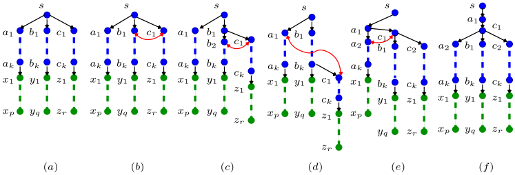
We now describe a sequence of $m$ edge insertions for which SDFS3 takes $\Theta(m^{2})$ time. Consider a graph $G=(V,E)$ where the set of vertices $V$ is divided into two sets $V^{\prime}$ and $I$, each of size $\Theta(n)$. The vertices in $V^{\prime}$ are connected in the form of a three chains (see Figure 10 (a)) and the vertices in $I$ are isolated vertices. Thus, it is sufficient to describe only the maintenance of DFS tree for the vertices in set $V^{\prime}$, as the vertices in $I$ will exist as isolated vertices connected to the dummy vertex $s$ in the DFS tree (recall that $s$ is the root of the DFS tree).

We divide the sequence of edge insertions into $k$ phases, where each phase is further divided into $k$ stages. At the beginning of each phase, we identify three chains having vertex sets from the set $V^{\prime}$, namely $A=\{a_{1},...,a_{k}\}$, $X=\{x_{1},...,x_{p}\}$ in the first chain, $B=\{b_{1},...,b_{l}\}$ and $Y=\{y_{1},...,y_{q}\}$ in the second chain and $C=\{c_{1},...,c_{k}\}$, $Z=\{z_{1},...,z_{r}\}$ in the third chain as shown in Figure 10 (a). The constants $k,p,q,r=\Theta(\sqrt{m})$ such that $q>r+k$ and $p\approx q+r+k$. We then add $e_{Z}=\Theta(m)$ edges to the set $Z$, $e_{y}=e_{z}+k+1$ edges to $Y$ and $e_{x}=e_{z}+e_{y}$ edges to $X$, which is overall still $\Theta(m)$. The size of $A$ and $C$ is $k$ in the first phase and decreases by $1$ in each the subsequent phases. Figure 10 (a) shows the DFS tree of the initial graph.

Now, the first stage of the phase starts with addition of the cross edge $(b_{1},c_{1})$ as shown in Figure 10 (b). Clearly, $s$ is the LCA of the inserted edge and SDFS3 would rebuild the smaller of the two subtrees $T(b_{1})$ and $T(c_{1})$. Since $q>r$, SDFS3 would hang $T(c_{1})$ through edge $(b_{1},c_{1})$ and perform partial DFS on $T(c_{1})$ requiring to process $\Theta(m)$ edges in $Z$. This completes the first stage with the resultant DFS tree shown in the Figure 10 (c). This process continues for $k$ stages, where in $i^{th}$ stage, $T(c_{1})$ would initially hang from $b_{i-1}$ and $(b_{i},c_{1})$ would be inserted. The DFS tree at the end of $k^{th}$ stage is shown in Figure 10 (d). At the end of $k$ stages, every vertex in $B$ is connected to the vertex $c_{1}$, hence we remove it from $C$ for the next phase. For this we first add the edge $(a_{1},c_{1})$. Since both $T(b_{1})$ and $T(a_{1})$ have approximately same number of vertices (as $p\approx q+r+k$), we add constant number of vertices (if required) to $Z$ from $I$ to ensure $T(b_{1})$ is rebuilt. The resultant DFS tree is shown in Figure 10 (e). Finally, we add $(a_{2},c_{1})$. Again both $T(c_{1})$ and $T(a_{2})$ have approximately same number of vertices, so we add constant number of vertices from $I$ to $X$ ensuring $T(a_{2})$ is rebuild as shown in Figure 10 (f). Note the similarity between Figures 10 (a) and 10 (f). In the next phase, the only difference is that $A^{\prime}=\{a_{2},...,a_{k}\}$, $C^{\prime}=\{c_{2},...,c_{k}\}$ and $s^{\prime}=c_{1}$. In each phase one vertex each from $A$ and $C$ are removed and constant number of vertices from $I$ are removed. Hence the phase can be repeated $k$ times.

Thus, we have $k$ phases each having $k$ stages. Further, in each stage we add a single cross edge forcing SDFS3 to process $\Theta(m)$ edges to rebuild the DFS tree. Thus, the total number of edges added to the graph is $k*k=\Theta(m)$ and the total time taken by ADFS1 is $k*k*\Theta(m)=\Theta(m^{2})$. Hence, we get the following theorem for any $n\leq m\leq{n\choose 2}$.

Figure 10: Example to demonstrate the tightness of the SDFS3. (a) Beginning of a phase with vertex sets $A$, $B$ and $X$. (b) Phase begins with addition of two vertex sets $C$ and $D$. The first stage begins by inserting a back edge $(a_{1},b_{k})$ and a cross edge $(b_{1},c_{k})$. (c) The rerooted subtree with the edges in $A\times X$ and $(b_{k},a_{1})$ as cross edges. (d) Final DFS tree after the first stage. (e) Final DFS tree after first phase. (f) New vertex sets $A^{\prime}$, $B^{\prime}$ and $X$ for the next phase.

Theorem D.1.

For each value of $n\leq m\leq{n\choose 2}$, there exists a sequence of $m$ edge insertions for which SDFS3 requires $\Theta(m^{2})$ time to maintain the DFS tree.

Remark: The worst case example mentioned above (say $G_{1}$) would also work without $X,Y$ and $Z$. Consider a second example (say $G_{2}$), where we take size of $A=2*k+2$,$B=k+1$ and $C=k$ and the vertices of $C$ have $\Theta(m)$ edges amongst each other. The same sequence of edge insertions would also force SDFS3 to process $\Theta(m^{2})$ edges. However, $G_{1}$ also ensures the same worst case bound for SDFS3 if it chooses the subtree with lesser edges instead of the subtree with lesser vertices, which is an obvious workaround of the example $G_{2}$. The number of edges $e_{x},e_{y}$ and $e_{z}$ are chosen precisely to counter that argument.

Appendix E Time Plots for experiments

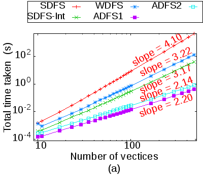
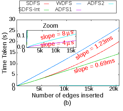
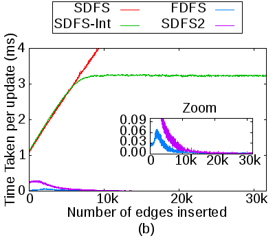
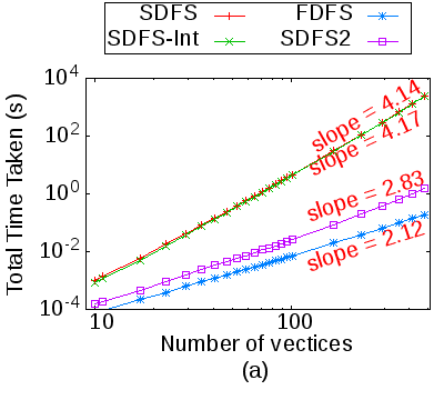
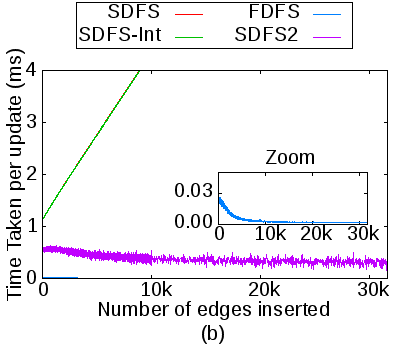
In this section we present the corresponding time plots for experiments performed earlier which were measured in terms of number of edges processed. The comparison of the existing incremental algorithms for random undirected graphs are shown in Figure 11. The comparison of the existing and proposed algorithms for random undirected graphs, random directed graphs and random DAGs are shown in Figure 12, Figure 13 and Figure 14 respectively.

Figure 11: For various existing algorithms, the plot shows (a) Total time taken (logarithmic scale) for insertion of $m={n\choose 2}$ edges for different values of $n$ , (b) Total time taken for $n=1000$ and up to $n\sqrt{n}$ edge insertions, (c) Time taken per update for $n=1000$ and up to $n\sqrt{n}$ edge insertions.

Figure 12: Comparison of existing and proposed algorithms on undirected graphs: (a) Total time taken for insertion of $m={n\choose 2}$ edges for different values of $n$. (b) Time taken per edge insertion for $n=1000$ and up to $n\sqrt{n}$ edge insertions.

Figure 13: Comparison of existing and proposed algorithms on directed graphs: (a) Total time taken for insertion of $m={n\choose 2}$ edges for different values of $n$ in logarithmic scale (b) Time taken per edge insertion for $n=1000$ and up to $n\sqrt{n}$ edge insertions.

Figure 14: Comparison of existing and proposed algorithms on DAGs: (a) Total time taken for insertion of $m={n\choose 2}$ edges for different values of $n$ in logarithmic scale (b) Time taken per edge insertion for $n=1000$ and up to $n\sqrt{n}$ edge insertions.

Appendix F Exact performance comparison for real graphs

The performance of different algorithms in terms of time and memory required on real undirected graphs and real directed graphs is shown in Table 4 and Table 5 respectively.

Dataset	$n$	$m|m^{*}$	$\frac{m}{n}|\frac{m}{m^{*}}$	ADFS1		ADFS2		SDFS3		SDFS2		SDFS		WDFS
ass733	7.72K	21.47K	2.78	0.08s	35.09M	0.15s	37.17M	2.73s	39.91M	51.16s	33.25M	1.51m	33.25M	3.99m	450.06M
		721.00	29.77	0.07s	35.11M	0.19s	36.66M	2.69s	31.98M	2.49s	32.77M	3.79s	32.77M	6.68s	385.61M
intTop	34.76K	107.72K	3.10	0.50s	160.14M	1.07s	162.58M	55.66s	150.17M	31.50m	152.12M	1.13h	148.95M	2.04h	2.57G
		18.27K	5.89	0.55s	160.80M	3.34s	169.44M	54.71s	150.84M	2.94m	151.81M	16.76m	146.00M	20.51m	2.56G
fbFrnd	63.73K	817.03K	12.82	10.26s	817.67M	22.39s	837.23M	25.06m	725.08M	5.75h	747.55M	41.80h	748.66M	33.48h	15.13G
		333.92K	2.45	10.46s	816.72M	1.41m	844.47M	24.59m	724.12M	1.43h	745.77M	22.17h	746.42M	12.40h	15.14G
wikiC	116.84K	2.03M	17.36	15.96s	1.89G	29.01s	1.91G	1.11h	1.65G	13.71h	1.67G	$>$100.00h	-	$>$100.00h	-
		205.59K	9.86	15.78s	1.89G	35.67s	1.91G	1.08h	1.65G	11.77h	1.67G	19.23h	1.67G	14.68h	38.50G
arxvTh	22.91K	2.44M	106.72	9.01s	2.10G	16.28s	2.11G	4.25m	1.81G	8.53h	1.81G	$>$100.00h	-	24.33h	39.48G
		210.00	11.64K	8.04s	2.61G	54.22s	2.77G	4.29m	2.34G	1.16m	2.33G	1.77m	2.33G	6.34h	3.94G
arxvPh	28.09K	3.15M	112.07	9.92s	2.69G	23.59s	2.71G	9.58m	2.33G	7.00h	2.32G	$>$100.00h	-	31.19h	50.80G
		2.26K	1.39K	8.15s	2.69G	1.12m	2.70G	9.61m	2.33G	14.02m	2.32G	26.11m	2.32G	7.18h	26.12G
dblp	1.28M	3.32M	2.59	16.31s	4.51G	26.12s	5.14G	$>$100.00h	-	$>$100.00h	-	$>$100.00h	-	$>$100.00h	-
		1.72M	1.93	16.93s	4.51G	31.17s	4.76G	$>$100.00h	-	$>$100.00h	-	$>$100.00h	-	$>$100.00h	-
youTb	3.22M	9.38M	2.91	17.29m	13.29G	1.02h	14.04G	$>$100.00h	-	$>$100.00h	-	$>$100.00h	-	$>$100.00h	-
		203.00	46.18K	23.44m	13.27G	42.08m	11.55G	$>$100.00h	-	18.67m	12.28G	18.62m	12.28G	80.93h	165.80G

Table 4: Comparison of time taken by different algorithms in seconds(s)/minutes(m)/hours(h) and memory required in kilobytes(K)/megabytes(M)/gigabytes(G) for maintaining incremental DFS on real undirected graphs.

Dataset	$n$	$m|m^{*}$	$\frac{m}{n}|\frac{m}{m^{*}}$	FDFS		SDFS3		SDFS2		SDFS
dncCoR	1.89K	5.52K	2.92	0.34s	9.22M	0.22s	8.61M	0.50s	8.50M	2.17s	8.50M
		4.01K	1.38	0.34s	9.22M	0.22s	8.62M	0.44s	8.48M	1.58s	8.47M
ucIrv	1.90K	20.30K	10.69	0.88s	17.47M	0.52s	15.30M	1.17s	22.94M	11.34s	15.17M
		20.12K	1.01	0.87s	17.47M	0.49s	15.28M	1.15s	15.16M	10.85s	15.14M
chess	7.30K	60.05K	8.22	26.03s	44.58M	13.39s	38.42M	34.00s	38.20M	4.46m	45.98M
		100.00	600.46	26.54s	52.48M	13.33s	43.75M	0.51s	43.94M	0.51s	44.64M
diggNw	30.40K	85.25K	2.80	2.23m	85.05M	2.98m	82.64M	8.03m	82.36M	32.33m	81.58M
		81.77K	1.04	2.32m	85.95M	3.21m	77.41M	8.77m	80.56M	27.70m	77.92M
asCaida	31.30K	97.84K	3.13	35.21s	97.45M	2.53m	87.00M	7.98m	87.95M	37.98m	86.48M
		122.00	801.98	35.19s	91.64M	1.99m	86.92M	2.82s	80.75M	2.80s	80.75M
wikiEl	7.12K	103.62K	14.55	16.21s	65.69M	16.02s	61.53M	41.27s	66.11M	13.83m	56.23M
		97.98K	1.06	16.27s	69.36M	16.24s	63.88M	41.16s	59.02M	14.18m	58.25M
slashDt	51.08K	130.37K	2.55	14.30m	127.23M	13.85m	123.47M	38.50m	116.55M	1.35h	122.88M
		84.33K	1.55	15.24m	126.61M	14.61m	122.08M	30.21m	116.94M	55.39m	122.12M
lnKMsg	27.93K	237.13K	8.49	9.52m	161.89M	5.22m	139.08M	12.51m	139.38M	2.02h	138.66M
		217.99K	1.09	9.51m	161.91M	5.38m	138.72M	12.35m	139.58M	2.07h	138.66M
fbWall	46.95K	264.00K	5.62	27.11m	200.05M	21.08m	175.05M	52.52m	174.80M	5.21h	174.81M
		263.12K	1.00	29.63m	200.03M	22.68m	175.03M	1.03h	174.77M	6.47h	174.80M
enron	87.27K	320.15K	3.67	10.32m	258.92M	16.00m	240.08M	58.40m	235.11M	11.63h	235.12M
		73.87K	4.33	11.31m	258.94M	16.80m	240.08M	29.48m	234.94M	2.64h	234.94M
gnutella	62.59K	501.75K	8.02	29.11m	345.39M	23.64m	286.66M	1.00h	284.78M	7.54h	284.88M
		9.00	55.75K	13.49m	288.19M	11.96m	245.27M	0.71s	245.27M	0.69s	245.28M
epinion	131.83K	840.80K	6.38	3.28h	556.69M	2.50h	487.06M	5.71h	478.86M	44.34h	479.22M
		939.00	895.42	3.09h	640.75M	3.04h	580.38M	1.95m	570.61M	1.95m	570.59M
digg	279.63K	1.73M	6.19	3.42h	1.13G	4.02h	986.58M	13.53h	977.58M	$>$100.00h	-
		1.64M	1.05	3.23h	1.13G	4.32h	986.58M	13.20h	977.55M	$>$100.00h	-
perLoan	89.27K	3.33M	37.31	9.39m	1.33G	1.11h	1.31G	4.80h	1.31G	$>$100.00h	-
		1.26K	2.65K	9.18m	1.33G	56.78m	1.31G	4.31m	1.31G	4.35m	1.31G
flickr	2.30M	33.14M	14.39	$>$100.00h	-	$>$100.00h	-	$>$100.00h	-	$>$100.00h	-
		134.00	247.31K	$>$100.00h	-	$>$100.00h	-	12.69m	15.00G	12.59m	15.00G
wikiHy	1.87M	39.95M	21.36	$>$100.00h	-	$>$100.00h	-	$>$100.00h	-	$>$100.00h	-
		2.20K	18.18K	$>$100.00h	-	$>$100.00h	-	1.44h	16.99G	1.63h	16.99G

Table 5: Comparison of performance of different algorithms in terms of time in seconds(s)/minutes(m)/hours(h) and memory required in kilobytes(K)/megabytes(M)/gigabytes(G) for maintaining incremental DFS on real directed graphs.

References

- [1] David Alberts, Giuseppe Cattaneo, and Giuseppe F. Italiano. An empirical study of dynamic graph algorithms. ACM Journal of Experimental Algorithmics, 2:5, 1997.
- [2] Paola Alimonti, Stefano Leonardi, and Alberto Marchetti-Spaccamela. Average case analysis of fully dynamic reachability for directed graphs. ITA, 30(4):305–318, 1996.
- [3] H. Bast, Kurt Mehlhorn, Guido Schäfer, and Hisao Tamaki. Matching algorithms are fast in sparse random graphs. Theory Comput. Syst., 39(1):3–14, 2006.
- [4] Surender Baswana, Shreejit Ray Chaudhury, Keerti Choudhary, and Shahbaz Khan. Dynamic DFS in undirected graphs: breaking the O(m) barrier. In SODA, pages 730–739, 2016.
- [5] Surender Baswana and Keerti Choudhary. On dynamic DFS tree in directed graphs. In MFCS, Proceedings, Part II, pages 102–114, 2015.
- [6] Surender Baswana and Shahbaz Khan. Incremental algorithm for maintaining DFS tree for undirected graphs. In ICALP, Proceedings, Part I, pages 138–149, 2014.
- [7] Béla Bollobás. The evolution of random graphs. Transactions of the American Mathematical Society, 286 (1):257–274, 1984.
- [8] Glencora Borradaile, Claire Mathieu, and Theresa Migler. Lower bounds for testing digraph connectivity with one-pass streaming algorithms. CoRR, abs/1404.1323, 2014.
- [9] Ulrik Brandes, Patrick Kenis, Jürgen Lerner, and Denise van Raaij. Computing wikipedia edit networks. 2009.
- [10] Giuseppe Cattaneo, Pompeo Faruolo, Umberto Ferraro Petrillo, and Giuseppe F. Italiano. Maintaining dynamic minimum spanning trees: An experimental study. Discrete Applied Mathematics, 158(5):404–425, 2010.
- [11] Munmun De Choudhury, Hari Sundaram, Ajita John, and Dorée Duncan Seligmann. Social synchrony: Predicting mimicry of user actions in online social media. In Proc. Int. Conf. on Computational Science and Engineering, pages 151–158, 2009.
- [12] Daniel Cordeiro, Grégory Mounié, Swann Perarnau, Denis Trystram, Jean-Marc Vincent, and Frédéric Wagner. Random graph generation for scheduling simulations. In 3rd International Conference on Simulation Tools and Techniques, SIMUTools ’10, Malaga, Spain - March 16 - 18, 2010, page 60, 2010.
- [13] Erik Demaine and Mohammad Taghi Hajiaghayi. Bigdnd: Big dynamic network data. http://projects.csail.mit.edu/dnd/, 2014.
- [14] Camil Demetrescu and Giuseppe F. Italiano. Experimental analysis of dynamic all pairs shortest path algorithms. ACM Trans. Algorithms, 2(4):578–601, 2006.
- [15] Paul Erdős and Alfréd Rényi. On random graphs I. Publicationes Mathematicae (Debrecen), 6:290–297, 1959.
- [16] P. Erdős and A Rényi. On the evolution of random graphs. In Publication of the Mathematical Institute of the Hungarian Academy of Sciences, pages 17–61, 1960.
- [17] Martin Farach-Colton, Tsan-sheng Hsu, Meng Li, and Meng-Tsung Tsai. Finding articulation points of large graphs in linear time. In Algorithms and Data Structures, WADS, pages 363–372, 2015.
- [18] Paolo Giulio Franciosa, Giorgio Gambosi, and Umberto Nanni. The incremental maintenance of a depth-first-search tree in directed acyclic graphs. Inf. Process. Lett., 61(2):113–120, 1997.
- [19] A. Frieze and M. Karoński. Introduction to Random Graphs. Cambridge University Press, 2015.
- [20] Vicenç Gómez, Andreas Kaltenbrunner, and Vicente López. Statistical analysis of the social network and discussion threads in Slashdot. In Proc. Int. World Wide Web Conf., pages 645–654, 2008.
- [21] Robert Görke, Pascal Maillard, Andrea Schumm, Christian Staudt, and Dorothea Wagner. Dynamic graph clustering combining modularity and smoothness. ACM Journal of Experimental Algorithmics, 18, 2013.
- [22] T. Hogg and K. Lerman. Social dynamics of Digg. EPJ Data Science, 1(5), 2012.
- [23] John E. Hopcroft and Richard M. Karp. An algorithm for maximum matchings in bipartite graphs. SIAM J. Comput., 2(4):225–231, 1973.
- [24] John E. Hopcroft and Robert Endre Tarjan. Efficient planarity testing. J. ACM, 21(4):549–568, 1974.
- [25] Raj Iyer, David R. Karger, Hariharan Rahul, and Mikkel Thorup. An experimental study of polylogarithmic, fully dynamic, connectivity algorithms. ACM Journal of Experimental Algorithmics, 6:4, 2001.
- [26] Abhabongse Janthong. Streaming algorithm for determining a topological ordering of a digraph. UG Thesis, Brown University, 2014.
- [27] S. Kapidakis. Average-case analysis of graph-searching algorithms. PhD Thesis, Princeton University, no. 286, 1990.
- [28] Bryan Klimt and Yiming Yang. The Enron corpus: A new dataset for email classification research. In Proc. European Conf. on Machine Learning, pages 217–226, 2004.
- [29] Jérôme Kunegis. Konect - the koblenz network collection. http://konect.uni-koblenz.de/networks/, October 2016.
- [30] Jure Leskovec, Daniel Huttenlocher, and Jon Kleinberg. Governance in social media: A case study of the Wikipedia promotion process. In Proc. Int. Conf. on Weblogs and Social Media, 2010.
- [31] Jure Leskovec, Jon Kleinberg, and Christos Faloutsos. Graph evolution: Densification and shrinking diameters. ACM Trans. Knowledge Discovery from Data, 1(1):1–40, 2007.
- [32] Jure Leskovec, Jon M. Kleinberg, and Christos Faloutsos. Graphs over time: densification laws, shrinking diameters and possible explanations. In Proceedings of the Eleventh ACM SIGKDD International Conference on Knowledge Discovery and Data Mining, Chicago, Illinois, USA, August 21-24, 2005, pages 177–187, 2005.
- [33] Jure Leskovec and Andrej Krevl. SNAP Datasets: Stanford large network dataset collection. http://snap.stanford.edu/data/, June 2014.
- [34] Michael Ley. The DBLP computer science bibliography: Evolution, research issues, perspectives. In Proc. Int. Symposium on String Processing and Information Retrieval, pages 1–10, 2002.
- [35] Paolo Massa and Paolo Avesani. Controversial users demand local trust metrics: an experimental study on epinions.com community. In Proc. American Association for Artificial Intelligence Conf., pages 121–126, 2005.
- [36] Guy Melancon. Just how dense are dense graphs in the real world?: A methodological note. In Proceedings of the 2006 AVI Workshop on BEyond Time and Errors: Novel Evaluation Methods for Information Visualization, BELIV ’06, pages 1–7, 2006.
- [37] Ulrich Meyer. Single-source shortest-paths on arbitrary directed graphs in linear average-case time. In Proceedings of the Twelfth Annual Symposium on Discrete Algorithms, January 7-9, 2001, Washington, DC, USA., pages 797–806, 2001.
- [38] Silvio Micali and Vijay V. Vazirani. An o(sqrt(v) e) algorithm for finding maximum matching in general graphs. In 21st Annual Symposium on Foundations of Computer Science, Syracuse, New York, USA, 13-15 October 1980, pages 17–27, 1980.
- [39] Alan Mislove. Online Social Networks: Measurement, Analysis, and Applications to Distributed Information Systems. PhD thesis, Rice University, Department of Computer Science, May 2009.
- [40] Alan Mislove, Hema Swetha Koppula, Krishna P. Gummadi, Peter Druschel, and Bobby Bhattacharjee. Growth of the flickr social network. In Proceedings of the 1st ACM SIGCOMM Workshop on Social Networks (WOSN’08), August 2008.
- [41] Rajeev Motwani. Average-case analysis of algorithms for matchings and related problems. J. ACM, 41(6):1329–1356, 1994.
- [42] Thomas C. O’Connell. A survey of graph algorithms under extended streaming models of computation. In Fundamental Problems in Computing: Essays in Honor of Professor Daniel J. Rosenkrantz, pages 455–476, 2009.
- [43] Tore Opsahl and Pietro Panzarasa. Clustering in weighted networks. Social Networks, 31(2):155–163, 2009.
- [44] Celso C. Ribeiro and Rodrigo F. Toso. Experimental analysis of algorithms for updating minimum spanning trees on graphs subject to changes on edge weights. In Experimental Algorithms, 6th International Workshop, WEA 2007, Rome, Italy, June 6-8, 2007, Proceedings, pages 393–405, 2007.
- [45] Matei Ripeanu, Adriana Iamnitchi, and Ian T. Foster. Mapping the gnutella network. IEEE Internet Computing, 6(1):50–57, 2002.
- [46] Jan Matthias Ruhl. Efficient Algorithms for New Computational Models. PhD thesis, Department of Computer Science, MIT, Cambridge, MA, 2003.
- [47] Dominik Schultes and Peter Sanders. Dynamic highway-node routing. In Experimental Algorithms, 6th International Workshop, WEA 2007, Rome, Italy, June 6-8, 2007, Proceedings, pages 66–79, 2007.
- [48] J.F. Sibeyn. Depth First Search on Random Graphs, volume 6 of Report -. Department of Computing Science, Umeå University, 2001.
- [49] Robert Endre Tarjan. Depth-first search and linear graph algorithms. SIAM J. Comput., 1(2):146–160, 1972.
- [50] Robert Endre Tarjan. Finding dominators in directed graphs. SIAM J. Comput., 3(1):62–89, 1974.
- [51] Robert Endre Tarjan. Dynamic trees as search trees via euler tours, applied to the network simplex algorithm. Mathematical Programming, 78:169–177, 1997.
- [52] Bimal Viswanath, Alan Mislove, Meeyoung Cha, and Krishna P. Gummadi. On the evolution of user interaction in facebook. In Proceedings of the 2nd ACM SIGCOMM Workshop on Social Networks (WOSN’09), August 2009.
- [53] Jeffery Westbrook and Robert Endre Tarjan. Maintaining bridge-connected and biconnected components on-line. Algorithmica, 7(5&6):433–464, 1992.
- [54] Beichuan Zhang, Raymond Liu, Daniel Massey, and Lixia Zhang. Collecting the internet as-level topology. SIGCOMM Computer Communication Review, 35(1):53–61, 2005.