A simple person’s approach to understanding the contagion condition for spreading processes on generalized random networks

To appear in “Spreading Dynamics in Social Systems”;
Eds. Sune Lehmann and Yong-Yeol Ahn, Springer Nature.

Abstract

We present derivations of the contagion condition for a range of spreading mechanisms on families of generalized random networks and bipartite random networks. We show how the contagion condition can be broken into three elements, two structural in nature, and the third a meshing of the contagion process and the network. The contagion conditions we obtain reflect the spreading dynamics in a clear, interpretable way. For threshold contagion, we discuss results for all-to-all and random network versions of the model, and draw connections between them.

I Introduction

Given a local contagion mechanism acting on a random network, and a seed set of nodes $\mathcal{N}_{0}$, we would like to know the answers to a series of increasingly specific questions:

1. Is a global spreading event possible? We’ll define a “global spreading event” as one that reaches a non-zero fraction of a network in the infinite limit.

2. If a global spreading event is possible, what’s the probability of one occurring?

3. What’s the distribution of final sizes for all spreading events?

4. Global or not, how does the spreading from the seed set $\mathcal{N}_{0}$ unfold in time?

Now, if we know the full time course of a spreading event (Q4) (see Gleeson and Cahalane (2007)), we evidently will be able to answer questions 1, 2, and 3. We might be tempted to take on only the more challenging analytical work and call it day (or appropriate time frame of suffering required). But it turns out to be useful to address each question separately

While we will take on these questions for simple model distillations only, their real-world counterparts are some of the most important ones we face. What’s the probability that a certain fraction of a population will contract influenza? Could an ecosystem collapse? Indeed, the biggest question for many systems is:

1. If we have limited knowledge of a network and limited control, how do we optimally facilitate or prevent spreading Lazarsfeld and Merton (1954); Watts and Dodds (2007)?

In this chapter, we’ll focus on Q1, determining the contagion condition for a range of contagion processes on random networks including bipartite ones. We will do so by plainly encoding the course of the spreading process itself into the contagion condition.

We will take the basic contagion mechanism to be one for which there are node states: Susceptible (S) and Infected (I). We will also prevent nodes from recovering or becoming susceptible; once nodes are infected, they remain so. In mathematical epidemiology, such models are referred to as SI, where S stands for Susceptible and I for Infected. Two other commonly studied models are SIR and SIRS, where a recovered immune state R is allowed for both and the possibility of cycling in the latter.

For the most part, we will be considering infinite random networks. If needed, we will define such networks as the limit of a one parameter family of networks (e.g., Erdös-Rényi networks with increasing $N$ and mean degree held constant). As a rough guide for simulations, using around $N=10^{4}$ nodes is typically sufficient for yield results that visually conform well to theoretical ones (e.g., fractional size of the largest component in Erdös-Rényi networks).

II Elements of simple contagion on random networks

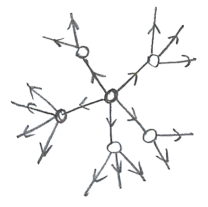
The key feature of random networks for spreading is that they are locally pure branching structures. This remains true for a large number of variations on random networks such as correlated random networks and bipartite affiliation graphs. Successful spreading away from a single seed (which could be one of many seeds) can only occur if nodes are susceptible when just one of their neighbors is infected (see Fig. 1). We will refer to these easily susceptible nodes as critical nodes (called vulnerable nodes in Watts (2002)). Denoting a network’s entire node set as $\Omega$, global spreading will only be possible if there is a connected subnetwork of critical nodes that forms a giant component, the critical mass network $\Omega_{\textnormal{crit}}$.

This set of critical nodes behaves in the same way as a critical mass one does for collective action Olson (1971); Granovetter (1978); Oliver et al. (1985); Oliver (1993) but there is now an internal dynamic. If one node is infected within the critical mass network $\Omega_{\textnormal{crit}}$, then spreading to some fraction of the critical mass network and beyond is possible, depending on the probablistic nature of the contagion process.

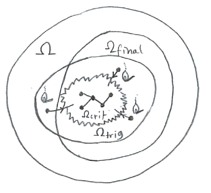
There are two other subnetworks that need to be characterized to understand spreading on random networks. First, containing the critical mass network and all non-critical nodes connected to the critical mass network is the triggering component, $\Omega_{\textnormal{trig}}$. Knowledge of this structure is required to determine the probability of a global spreading event Harris et al. (2014). Second, we have $\Omega_{\textnormal{final}}$ which is the extent of infection realized for any spreading event. For random networks, the distribution of the fractional size of $\Omega_{\textnormal{final}}$ will be either unimodal (the contagion process always succeeds) or bimodal (initial failure is possible).

If Fig. 2, we show how the three subnetworks $\Omega_{\textnormal{crit}}$, $\Omega_{\textnormal{trig}}$, and $\Omega_{\textnormal{final}}$ potentially overlap. A global spreading event is only possible if $\Omega_{\textnormal{crit}}$ takes up a non-zero fraction of the network. Some limiting cases allow for surprising kinds of robust-yet-fragile contagion, such as $\Omega_{\textnormal{crit}}$ being vanishingly small while any successful infection spreads to the full network Watts (2002).

Figure 1: Random networks are locally pure branching structures. For the initial stages of the spread shown, nodes can only experience the infection from a single neighbor. For spreading to take off from a simple seed, the network must contain a connected macroscopic critical mass network $\Omega_{\textnormal{crit}}$ of nodes susceptible to a single neighbor becoming infected.

Figure 2: One possible arrangement of the three essential subnetworks for a contagion process on a random network: the critical mass network $\Omega_{\textnormal{crit}}$, the triggering component $\Omega_{\textnormal{trig}}$, and the final extent of a global spreading process, $\Omega_{\textnormal{final}}$. In general, $\Omega_{\textnormal{crit}}\subset\Omega_{\textnormal{trig}}$, $\Omega_{\textnormal{crit}}\subset\Omega_{\textnormal{final}}$, and $\Omega_{\textnormal{trig}},\Omega_{\textnormal{final}}\subset\Omega.$

III The Contagion Condition

We would like to devise some kind of general, quick test algorithm into which we would be able to feed any contagion mechanism and any network, whether constructed or real. Such an algorithm would generate what we’ll call a Contagion Condition, and would only be worthwhile if it avoided simulating all possible spreading events and instead computed a composite test statistic. Upon running a system through our algorithm we would simply receive a “Yes” or “No”. Scaling up, we could then test an array of systems in parallel and for the “Yes” responses, we would proceed to explore those systems in detail (e.g., those cities which are susceptible to Zombie outbreaks Munz et al. (2009)).

III.1 Contagion condition for one-shot spreading processes

For random network models, our test algorithm can be formulated in a physically-minded way. We will step through the building of the contagion condition for one-shot, permanent infection spreading on generalized, uncorrelated random networks and then expand from there.

By one-shot spreading, we mean that each newly infected node has one chance in the next time step to infect its uninfected neighbors. That is, if node $i$ fails to infect a specific neighbor $i^{\prime}$, then $i$ cannot attempt to infect $i^{\prime}$ again in any following time step. Permanent infection means that nodes do not recover.

For a node $i$ with degree $k$, we will write $i$’s probability of infection given $j$ of its neighbors are infected as $B_{kj}$. While our focus on the initial spread on random networks means we need only consider the probability nodes are infected by one of their neighbors, $B_{k1}$, we must consider the response to multiple simultaneous infections for later stages of global spreading on random networks Gleeson and Cahalane (2007); Gleeson (2008), more complicated contagion mechanisms, and, more importantly if we care about the real world, networks with non-zero clustering Watts and Strogatz (1998); Newman (2003).

As is often the case with networks, we open up better ways to understand and explain phenomena if we focus on edges rather than nodes. This is not entirely natural as for many problems we are ultimately concerned with how nodes behave and, for contagion especially, we can readily map ourselves directly onto individual nodes (will my next movie fail?). But once we lose this anchoring and shift to thinking first about edges with nodes in the background, clearer paths emerge.

So, instead of framing spreading as rooted in node infection rates, we consider the dynamics of infected edges. For our purposes, an infected edge will be one emanating from an infected node, and we will have to consider direction even for undirected networks.

We need to determine one number for our system, what we’ll call the gain ratio, $\mathbf{R}$ Dodds et al. (2011). We define $\mathbf{R}$ as the expected number of newly infected edges that will be generated by a single infected edge leading to an uninfected node. (In epidemiology, the gain ratio would be equivalent to the reproduction number, $R_{0}$.)

For the moment, let’s assume we have computed $\mathbf{R}$ for a system. Because sparse random networks are locally pure branching structures (see Fig. 1), the spread emanating from a single seed will also be a simple branching one. Early on, there will be no interactions between any two newly infected edges leading to the same uninfected node.

The fraction of newly infected edges at time $t$, $f_{(\cdot)}^{\textnormal{inf}}(t)$, must then follow an elementary evolution:

$$f_{(\cdot)}^{\textnormal{inf}}(t)=\mathbf{R}f_{(\cdot)}^{\textnormal{inf}}(t-1).$$ (1)

The subscript for the count $f^{\textnormal{inf}}$ will indicate the edge’s type which for our initial system is irrelevant, hence $(\cdot)$.

The early growth will therefore be exponential with

$$f_{(\cdot)}^{\textnormal{inf}}(t)=\mathbf{R}^{t}f_{(\cdot)}^{\textnormal{inf}}(0),$$ (2)

where $f_{(\cdot)}^{\textnormal{inf}}(0)$ equals the degree of the seed node. We might guess that we can write down the exact evolution as $f_{(\cdot)}^{\textnormal{inf}}(t)=\mathbf{R}^{t}f_{(\cdot)}^{\textnormal{inf}}(0),$ but the initial step is sneakily different. Well get to this issue later on.

Global spreading will evidently be possible only if

$$\mathbf{R}>1,$$ (3)

and this very simple criterion will be our Contagion Condition.

The above equations maintain the same form if we consider not one seed but a random seed set taking up a non-zero fraction of the random network. Writing $\rho_{t}$ as the fraction of edges emanating from newly infected nodes at time $t$, we have, again for the initial phase of spreading:

$$\rho_{t}=\mathbf{R}\rho_{t-1},$$ (4)

which leads to

$$\rho_{t}=\mathbf{R}^{t}\rho_{0}.$$ (5)

We now determine the gain ratio $\mathbf{R}$ for the simple class of one-shot contagion on random network systems. In doing so, we show that the Contagion Condition is worthwhile beyond being a simple diagnostic as, with the right treatment, it can be also seen to carry physical intuition.

In determining $\mathbf{R}$, there are three (3) pieces to consider: two are structural and a function of the network, and the third couples the contagion mechanism to the network.

1. We start on an edge that has just become infected and look toward the uninfected node that has now become exposed. The properly normalized probability that this node has degree $k$ is

   $$Q_{k}=\frac{kP_{k}}{\langle k\rangle}$$ (6)

   because each degree $k$ node can be reached along its $k$ edges. This skewing of the degree distribution is a result of some renown as it drives the Simon-like rich-get-richer models of network growth of Price de Solla Price (1965, 1976) and Barabási and Albert Barabási and Albert (1999), and also underlies the friendship paradox and its generalizations Eom and Jo (2014); Momeni and Rabbat (2016): Your friends are quite likely to be different from you, and often in disappointing ways such as by having more friends or wealth on average.

2. Second, we have the action of contagion mechanism. As have already defined, with probability $B_{k1}$ the node of degree $k$ is infected by the single incoming infected edge. With probability $1-B_{k1}$, the infection fails.

3. Depending on whether or not the infection is successful, we know that in the next time step the contagion mechanism will generate either 0 or $k-1$ new infected edges.

Putting these pieces together, we have

$$\mathbf{R}=\sum_{k=0}^{\infty}\underbrace{\frac{kP_{k}}{\langle k\rangle}}_{\mbox{ \scriptsize\begin{tabular}[]{l}prob. of\\ connecting to\\ a degree $k$ node\\ \end{tabular} }}\bullet\underbrace{B_{k1}}_{\mbox{\scriptsize\begin{tabular}[]{l}Prob. of\\ infection\end{tabular} }}\bullet\underbrace{(k-1)}_{\mbox{\scriptsize\begin{tabular}[]{l}\# outgoing\\ infected\\ edges\end{tabular} }}$$ (15)

$$+\ \sum_{k=0}^{\infty}\underbrace{\frac{kP_{k}}{\langle k\rangle}}_{\mbox{ \scriptsize\begin{tabular}[]{l}prob. of\\ connecting to\\ a degree $k$ node\\ \end{tabular} }}\bullet\underbrace{(1-B_{k1})}_{\mbox{\scriptsize\begin{tabular}[]{l}Prob. of\\ no infection\end{tabular} }}\bullet\underbrace{(\ 0\ )}_{\mbox{\scriptsize\begin{tabular}[]{l}\# outgoing\\ infected\\ edges\end{tabular} }}$$ (24)

The second piece evaporates and we have our contagion condition:

$$\ \mathbf{R}=\sum_{k=0}^{\infty}\frac{kP_{k}}{\langle k\rangle}\bullet B_{k1}\bullet(k-1)>1.\$$ (25)

Again, the value here is that this structure of $\mathbf{R}$ encodes the contagion mechanism in a clear way. As such, we resist any urge to rearrange the form of Eq. (25) for a more elegant form. As we move to more general systems, the three part form of two pieces for the network and one for the contagion mechanism will be maintained, and the criterion of a single number exceeding unity, $\mathbf{R}>1$, will elevate to being the largest eigenvalue of a gain ratio matrix exceeding unity.

We now move through a few examples of other kinds of systems involving contagion mechanisms acting on network structures.

III.2 Contagion condition for multiple-shot spreading processes

We have presumed a one-shot contagion process in our derivation of Eq. (25). In loosening this restriction to spreading processes that may involve repeated attempts to infect a node with the possible recovery of the infected node allowed as well, we can compute $B_{k1}$ as the long term probability of infection. The form of gain ratio remains the same and therefore so does the contagion condition given in Eq. (25).

III.3 Remorseless spreading and the giant component condition

We step back from contagion momentarily to show that we can also determine whether or not a random network has a giant component. This is now a structural test absent any processes. A network will have a giant component if it is, on average, locally expanding. That is, if we travel along a randomly chosen edge, we will reach a node which has, on average, more than one other edge emanating from it. But this is just a remorseless version of our one-shot contagion mechanism, one where infection always succeeds, i.e., $B_{k1}=1$.

Setting $B_{k1}=1$ in Eq. (25), we have the giant component condition:

$$\mathbf{R}=\sum_{k=0}^{\infty}\frac{kP_{k}}{\langle k\rangle}\bullet(k-1)>1,$$ (26)

where we have again used the physical sense of a gain ratio.

III.4 Simple contagion on generalized random networks

If $B_{k1}=B<1$, A fraction (1-$B$) of all edges will not transmit infection, and the contagion condition becomes

$$\mathbf{R}=\sum_{k=0}^{\infty}\frac{kP_{k}}{\langle k\rangle}\bullet B\bullet(k-1)>1.$$ (27)

This is a bond percolation model Stauffer and Aharony (1992), and Eq. (27) can be seen as a giant component condition for a network with (1-$B$) of its edges removed. The resultant network has a degree distribution $\tilde{P}_{k}=B^{k}\sum_{i=k}^{\infty}\binom{i}{k}(1-B)^{i-k}P_{i},$ and evidently, as $B$ decreases, only increasingly more connected networks will be able to facilitate spreading.

III.5 Other routes to determining the contagion and giant component conditions

There are many other ways to arrive at the contagion condition in Eq. (25) and the giant component condition in Eq. (26). The path taken affects the form of the condition and may limit understandability Dodds et al. (2011). For example, the giant component condition was determined by Molloy and Reed Molloy and Reed (1995) in 1995 and presented as

$$\sum_{k=0}^{\infty}k(k-2)P_{k}>0.$$ (28)

While equivalent to Eq. (26), the framing of local expansion is obscured.

For a simple spreading mechanism with $B_{k1}=B$, Newman Newman (2003), for example, used generatingfunctionology methods Wilf (2006) to first determine the average size of finite components and then find when this quantity diverged. For Granovetter’s social contagion threshold model on random networks Granovetter (1978), Watts took the same approach Watts (2002). This size divergence is a hallmark of phase transitions in statistical mechanical systems in general, and while it can be used to find the critical point, doing so would ideally be at the level of a consistency check.

For the giant component condition, a somewhat more direct approach using generating functions Newman et al. (2001) is based on the probability distribution that the node at the randomly chosen end of a randomly chosen edge has $k$ other edges is

$$R_{k}=Q_{k+1}=\frac{1}{{\langle k\rangle}}(k+1)P_{k+1}.$$ (29)

Writing the generating function for the degree distribution as $F_{P}(x)=\sum_{k=0}^{\infty}P_{k}x^{k}$, we have $F_{R}(x)=F^{\prime}_{P}(x)/F^{\prime}_{P}(1),$ where we have used $\langle k\rangle=F^{\prime}_{P}(1)$, an elementary result for determining averages with generating functions Wilf (2006). The average number of other edges found at a randomly-arrived-at node is $F^{\prime}_{R}(1)=F^{\prime\prime}_{P}(1)/F^{\prime}_{P}(x)=\frac{\langle k(k-1)\rangle}{\langle k\rangle}.$ This is exactly our gain ratio and we now have

$$\frac{\langle k(k-1)\rangle}{\langle k\rangle}>1$$ (30)

for the giant component condition. Again, while Eqs. 26 and 30 are equivalent, the latter does not have an immediate physical interpretation—it’s just a condition.

III.6 Simple contagion on generalized directed random networks

Figure 3: For general directed networks, a node has $k_{\textnormal{i}}$ incident edges and $k_{\textnormal{o}}$ emanating edges governed by a a joint distribution $P_{k_{\textnormal{i}},k_{\textnormal{o}}}$.

For purely directed networks, we allow each node to have an in-degree $k_{\textnormal{i}}$ and an out-degree $k_{\textnormal{o}}$ with probability $P_{k_{\textnormal{i}},k_{\textnormal{o}}}$ (see Fig. 3). The same arguments that gave us Eq. (25) now end with:

$$\mathbf{R}=\sum_{k_{\textnormal{i}}=0}^{\infty}\sum_{k_{\textnormal{o}}=0}^{\infty}\frac{k_{\textnormal{i}}P_{k_{\textnormal{i}},k_{\textnormal{o}}}}{\langle k_{\textnormal{i}}\rangle}\bullet B_{k_{\textnormal{i}},1}\bullet k_{\textnormal{o}}>1.$$ (31)

The three components of the contagion condition have the same interpretation as before.

III.7 Simple contagion on mixed, correlated random networks

Figure 4: Nodes in mixed random networks have $k_{\textnormal{u}}$ undirected edges, $k_{\textnormal{i}}$ incident edges, and $k_{\textnormal{o}}$ emanating edges. Node degree is represented by the vector $\vec{k}=[\ k_{\textnormal{u}}\ k_{\textnormal{i}}\ k_{\textnormal{o}}\ ]^{\textnormal{T}}$ and degrees are sampled from a joint distribution $P_{\vec{k}}$.

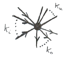
We jump to a more complex possibility of mixed random networks with a combination of directed and undirected (or bidirectional) edges as well as arbitrary degree-degree correlations between nodes, as introduced in  Boguñá and Ángeles Serrano (2005).

Nodes may have three types of edges: $k_{\textnormal{u}}$ undirected edges, $k_{\textnormal{i}}$ incoming directed edges, and $k_{\textnormal{o}}$ outgoing directed edges. The degree distribution is now a function of a three-vector:

$$P_{\vec{k}}\ \mbox{where}\ \vec{k}=[\ k_{\textnormal{u}}\ \ k_{\textnormal{i}}\ \ k_{\textnormal{o}}\ ]^{\textnormal{T}}.$$ (32)

As for directed networks, we require in- and out-degree averages to match up: $\langle k_{\textnormal{i}}\rangle=\langle k_{\textnormal{o}}\rangle.$ We add two point correlations per Boguñá and Ángeles Serrano (2005); Dodds et al. (2011) through three conditional probabilities:

• $P^{(\textnormal{{u})}}(\vec{k}\,|\,\vec{k}^{\prime})$ = probability that an undirected edge leaving a degree $\vec{k}^{\prime}$ nodes arrives at a degree $\vec{k}$ node.

• $P^{(\textnormal{{i})}}(\vec{k}\,|\,\vec{k}^{\prime})$ = probability that an edge leaving a degree $\vec{k}^{\prime}$ nodes arrives at a degree $\vec{k}$ node is an in-directed edge relative to the destination node.

• $P^{(\textnormal{{o})}}(\vec{k}\,|\,\vec{k}^{\prime})$ = probability that an edge leaving a degree $\vec{k}^{\prime}$ nodes arrives at a degree $\vec{k}$ node is an out-directed edge relative to the destination node.

We now require more refined (detailed) balance along both undirected and directed edges (see Fig. 5). Specifically, we must have Boguñá and Ángeles Serrano (2005); Dodds et al. (2011): $P^{(\textnormal{{u})}}(\vec{k}\,|\,\vec{k}^{\prime})\frac{k_{\textnormal{u}}^{\prime}P(\vec{k}^{\prime})}{\langle k_{\textnormal{u}}^{\prime}\rangle}=P^{(\textnormal{{u})}}(\vec{k}^{\prime}\,|\,\vec{k})\frac{k_{\textnormal{u}}P(\vec{k})}{\langle k_{\textnormal{u}}\rangle},$ and $P^{(\textnormal{{i})}}(\vec{k}\,|\,\vec{k}^{\prime})\frac{k_{\textnormal{o}}^{\prime}P(\vec{k}^{\prime})}{\langle k_{\textnormal{o}}^{\prime}\rangle}=P^{(\textnormal{{o})}}(\vec{k}^{\prime}\,|\,\vec{k})\frac{k_{\textnormal{i}}P(\vec{k})}{\langle k_{\textnormal{i}}\rangle}.$

For all example systems so far, the gain ratio has been a single number. For mixed random networks, infections along directed edges may cause infections along undirected edges and so on. We will need to count undirected and directed edge infections separately, the growth of infections for a one-shot contagion process will obey the following dynamic:

$$\left[\begin{array}[]{c}f_{\vec{k}}^{\textnormal{({u})}}(t+1)\\ f_{\vec{k}}^{\textnormal{({o})}}(t+1)\end{array}\right]=\sum_{\vec{k}^{\prime}}\textbf{R}_{\vec{k}\vec{k}^{\prime}}\left[\begin{array}[]{c}f_{\vec{k}^{\prime}}^{\textnormal{({u})}}(t)\\ f_{\vec{k}^{\prime}}^{\textnormal{({o})}}(t)\end{array}\right],$$ (33)

where we now identify a gain ratio tensor:

$$\textbf{R}_{\vec{k}\vec{k}^{\prime}}=$$ (37)

$$\left[\begin{array}[]{ll}P^{(\textnormal{{u})}}(\vec{k}\,|\,\vec{k}^{\prime})\bullet B_{\vec{k}\vec{k}^{\prime}}\bullet(k_{\textnormal{u}}-1)&P^{(\textnormal{{i})}}(\vec{k}\,|\,\vec{k}^{\prime})\bullet B_{\vec{k}\vec{k}^{\prime}}\bullet k_{\textnormal{u}}\\ P^{(\textnormal{{u})}}(\vec{k}\,|\,\vec{k}^{\prime})\bullet B_{\vec{k}\vec{k}^{\prime}}\bullet k_{\textnormal{o}}&P^{(\textnormal{{i})}}(\vec{k}\,|\,\vec{k}^{\prime})\bullet B_{\vec{k}\vec{k}^{\prime}}\bullet k_{\textnormal{o}}\end{array}\right].$$

For a gain ratio matrix or tensor, our contagion condition is now a test of whether or not the largest eigenvalue exceeds 1.

Figure 5: For mixed random networks, node degree correlations may be measured along undirected and/or directed edges.

III.8 Contagion on correlated random networks with arbitrary node and edge types

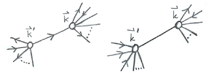
We make one last step of generalization for correlated random networks Dodds et al. (2011). As per Fig. 6, we allow arbitrary types of nodes and edges along with arbitrary correlations between node-edge pairs. For multi-shot contagion, we have

$$f_{\vec{\alpha}}(d+1)=\sum_{\vec{\alpha}^{\prime}}R_{\vec{\alpha}\vec{\alpha}^{\prime}}f_{\vec{\alpha}^{\prime}}(d)$$ (38)

where $R_{\vec{\alpha}\vec{\alpha}^{\prime}}$ is the gain ratio matrix and has the form:

$$R_{\vec{\alpha}\vec{\alpha}^{\prime}}=P_{\vec{\alpha}\vec{\alpha}^{\prime}}\bullet k_{\vec{\alpha}\vec{\alpha}^{\prime}}\bullet B_{\vec{\alpha}\vec{\alpha}^{\prime}}.$$ (39)

Here,

• $P_{\vec{\alpha}\vec{\alpha}^{\prime}}$ = conditional probability that a type $\lambda^{\prime}$ edge emanating from a type $\nu^{\prime}$ node leads to a type $\nu$ node.

• $k_{\vec{\alpha}\vec{\alpha}^{\prime}}$ = potential number of newly infected edges of type $\lambda$ emanating from nodes of type $\nu$.

• $B_{\vec{\alpha}\vec{\alpha}^{\prime}}$ = probability that a type $\nu$ node is eventually infected by a single infected type $\lambda^{\prime}$ link arriving from a neighboring node of type $\nu^{\prime}$.

Finally, we can write down our generalized contagion condition as:

$$\max{|\mu|}:\mu\in\sigma\left(\mathbf{R}\right)>1,$$ (40)

where $\sigma(\mathbf{R})$ denotes the eigenvalue spectrum of $\mathbf{R}$.

Figure 6: Element of a general correlated random network where edges and nodes may take on arbitrary characteristics. Node and edge type are specified as $\alpha=(\nu,\lambda)$.

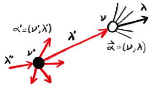
III.9 Simple contagion on bipartite random networks

Figure 7: Example of a bipartite affiliation network and the induced networks. Center: A small story-trope bipartite graph. The induced trope network and the induced story network are on the left and right. The dashed edge in the bipartite affiliation network indicates an edge added to the system, resulting in the dashed edges being added to the two induced networks.

Figure 8: Spreading on a random bipartite network can be seen as bouncing back and forth between the two connected populations. The gain ratio for simple contagion on a bipartite random network is the product of two gain ratios as shown in Eq. (III.9).

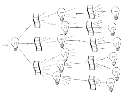
Bipartite networks (or affiliation graphs) connect two populations through some association, and induce networks within each population Newman et al. (2001); Ahn et al. (2011); Teng et al. (2012); Hidalgo et al. (2007); Goh et al. (2007); García-Pérez et al. (2014). Bipartite structures and variants are natural representations of many real networked systems with a classic example being boards and directors. The induced distributions are formed by connecting all pairs of boards that share at least one director and all pairs of directors that belong to the same board.

Base models for real bipartite systems are random bipartite networks which are formed by randomly connecting two populations with specified degree distributions. Random bipartite networks are able to reproduce induced degree distributions, which may be non-trivial in form Newman et al. (2001).

To help with our analysis, we’ll consider a random bipartite network between stories and tropes tvt . Each story contains one or more trope, and each trope is part of one more stories. Stories sharing tropes are then linked as are tropes found in the same story. In Fig. 7, we show a small example (center) along with the induced trope-trope and story-story networks.

For spreading between stories we may wish to imagine we’re in the BookWorld of the Thursday Next series Fforde (2001).

We’ll use this notation for our two inter-affiliated types: for stories and for tropes.

Consider a story-trope system with $N_{\textnormal{\faFilm}}$ denoting the number of stories, $N_{\textnormal{\faLightbulbO}}$ the number of tropes, and $m_{\textnormal{\faFilm},\textnormal{\faLightbulbO}}$ the number of edges connecting stories and tropes.

Let’s have some underlying distributions for numbers of affiliations: $P^{(\textnormal{\faFilm})}_{k}$ (a story has $k$ tropes) and $P^{(\textnormal{\faLightbulbO})}_{k}$ (a trope is in $k$ stories).

Some bookkeeping arises with balance requirements. Writing $\langle k\rangle_{\textnormal{\faFilm}}$ as the average number of tropes per story, and $\langle k\rangle_{\textnormal{\faLightbulbO}}$ as the average number of stories containing a given trope, we must have: $N_{\textnormal{\faFilm}}\cdot\langle k\rangle_{\textnormal{\faFilm}}=m_{\textnormal{\faFilm},\textnormal{\faLightbulbO}}=N_{\textnormal{\faLightbulbO}}\cdot\langle k\rangle_{\textnormal{\faLightbulbO}}.$

Let’s first get to the giant component condition before talking about contagion.

Just as for random networks, we focus on edges begetting edges, and we will need the distributions analogous to $Q_{k}$, Eq. (6). We randomly select an edge connecting a story to a trope . Traveling from the trope to the story, we have that the probability the story contains $k$ total tropes is:

$$Q^{(\textnormal{\faFilm})}_{k}=\frac{kP^{(\textnormal{\faFilm})}_{k}}{\sum_{j=0}^{N_{\textnormal{\faFilm}}}jP^{(\textnormal{\faFilm})}_{j}}=\frac{kP^{(\textnormal{\faFilm})}_{k}}{\langle k\rangle_{\textnormal{\faFilm}}}.$$ (41)

Heading instead towards the trope , we find the probability that the trope is in $k$ total stories is

$$Q^{(\textnormal{\faLightbulbO})}_{k}=\frac{kP^{(\textnormal{\faLightbulbO})}_{k}}{\sum_{j=0}^{N_{\textnormal{\faLightbulbO}}}jP^{(\textnormal{\faLightbulbO})}_{j}}=\frac{kP^{(\textnormal{\faLightbulbO})}_{k}}{\langle k\rangle_{\textnormal{\faLightbulbO}}}.$$ (42)

To determine the giant component condition for the induced network of stories (to choose a side), let’s start with a randomly chosen edge and travel from the story to the trope. As shown starting on the left of Fig. 8, we hit the trope and then travel to the other stories containing that trope. This bouncing back and forth between tropes and stories continues and because the connections are random and if the system is large enough, no story or trope is returned to early on. Just as for random networks, there are no short loops (technically, finitely many in the infinite limit).

We are thus able to depict the expanding branching in Fig. 8 and we can see that the giant component condition will involve the product of the gain ratio for each distribution.

$$\mathbf{R}=\mathbf{R}_{\textnormal{\faFilm}}\cdot\mathbf{R}_{\textnormal{\faLightbulbO}}=$$

$$\left[\sum_{k=0}^{\infty}\frac{kP^{(\textnormal{\faFilm})}_{k}}{\langle k\rangle_{\textnormal{\faFilm}}}\bullet(k-1)\right]\left[\sum_{k=0}^{\infty}\frac{kP^{(\textnormal{\faLightbulbO})}_{k}}{\langle k\rangle_{\textnormal{\faLightbulbO}}}\bullet(k-1)\right]>1$$

As for gain ratios for random networks we can arrive at this result through the use of generating functions and other approaches. Regardless of the path, more mathematically pleasing variants are always available such as Newman et al. (2001):

$$\sum_{k=0}^{\infty}\sum_{k^{\prime}=0}^{\infty}kk^{\prime}(kk^{\prime}-k-k^{\prime})P^{(\textnormal{\faFilm})}_{k}P^{(\textnormal{\faLightbulbO})}_{k^{\prime}}=0,$$ (44)

but, again, we have stripped the physics away.

Introducing a simple contagion can be done as before by allowing tropes to infect other tropes in the same story (with probability $B_{k1}^{(\textnormal{\faLightbulbO})}$) and stories to affect other stories if they share a trope (with probability $B_{k1}^{(\textnormal{\faFilm})}$) We adjust Eq. (III.9) to obtain:

$$\mathbf{R}=\mathbf{R}_{\textnormal{\faFilm}}\cdot\mathbf{R}_{\textnormal{\faLightbulbO}}=$$

$$\left[\sum_{k=0}^{\infty}\frac{kP^{(\textnormal{\faFilm})}_{k}}{\langle k\rangle_{\textnormal{\faFilm}}}\bullet B_{k1}^{(\textnormal{\faFilm})}\bullet(k-1)\right]$$

$$\times\left[\sum_{k=0}^{\infty}\frac{kP^{(\textnormal{\faLightbulbO})}_{k}}{\langle k\rangle_{\textnormal{\faLightbulbO}}}\bullet B_{k1}^{(\textnormal{\faLightbulbO})}\bullet(k-1)\right]>1$$

III.10 Threshold contagion on generalized random networks

We turn to our last example: threshold contagion, an important simple model of social contagion Schelling (1971, 1973, 1978); Granovetter (1978); Granovetter and Soong (1983, 1986, 1988); Watts (2002). In basic threshold contagion models, all individuals observe the infection status of their neighbors at each time step, and become infected if their internal threshold is exceeded. In the present and following section, we will explore the contagion condition for threshold models on all-to-all networks and random networks, and examine the early course of a global spreading event reflecting on the nature of early adopters.

In Granovetter’s mean-field or all-to-all network version Granovetter (1978), individuals are always aware of the overall fraction of the population that is infected. We write the fraction of the population that is infected at time $t$ as $a_{t}$. If we have a general threshold distribution $f(\phi)$, then the fraction of the population whose threshold will be exceeded at time $t$ and hence be infected at time $t+1$ is:

$$\phi_{t+1}=\int_{0}^{\phi_{t}}f(u)\textnormal{d}u=\left.F(u)\right|_{0}^{\phi_{t}}=F(\phi_{t})-F(0)$$ (46)

where $F$ is the cumulative distribution of $f$ (if $F(0)>0$, then the system has nodes that will always be on regardless of the state of others). Thus, we have system whose dynamics are described by a map of the unit interval. We are interested in small seeds for the mean-field version, i.e., $\phi_{0}\rightarrow 0$. In this limit, global spreading occurs if (1) $F(0)>0$ meaning the population will always activate spontaneously, or (2) $\phi=0$ is a fixed point but is unstable (meaning $F(0)=0$ and $F^{\prime}(0)>1$). If $\phi=0$ is a stable fixed point (meaning $F(0)=0$ and $F^{\prime}(0)<1$), then spreading may still occur but not for vanishingly small seeds. Perhaps surprisingly, the same process on a network may give rise to spreading from a single seed, as we explain this in the next section.

For the random network version due to Watts Watts (2002), and again taking a general threshold distribution $f(\phi)$ a degree $k$ node will be part of the critical mass network with probability:

$$B_{k1}=\int_{0}^{1/k}f(\phi)\textnormal{d}\phi.$$ (47)

The gain ratio remains the same as the one given in Eq. (25).

We now link the contagion conditions for the all-to-all network and random network versions of social contagion.

III.11 Connecting the contagion condition for all-to-all and random networks for threshold contagion

Figure 9: Plots comparing the behavior of the model on all-to-all networks (plots A and C) and random networks (B and D) for two different example threshold distributions. The insets to plots A and C show the two underlying threshold distributions, which are unimodal and bimodal respectively, and the corresponding cumulative distributions are presented in the main plots of A and C. Plots B and D show global spreading event intervals for random networks with the same threshold distributions as A and C respectively. The black lines in B and D indicate the average size of global spreading events that exceed $0.05N$, and the dashed lines the average size of the largest critical mass network (sizes are normalized by $N$) The threshold distribution in plot A leads to a bounded global spreading event interval on random networks while the distribution in plot C leads to an unbounded one. In plot D, the average size of the largest critical mass network decays to 0 as $\langle k\rangle\rightarrow\infty$. The results in plots B and D are derived from $10^{3}$ networks with $N=10^{4}$ and one seed per network.

We make the simple observation that if we examine the threshold model’s behavior on a random network and allow the average degree $\langle k\rangle$ to increase, then the results will tend towards what we would observe on an all-to-all network. Since the limiting behavior of the contagion model on all-to-all networks is governed by the presence or absence of fixed points of the cumulative threshold distribution $F$, we are therefore able to state what the model’s behavior on random networks must tend towards as $\langle k\rangle$ increases based solely on the form of $F$.

We consider two examples of threshold distribution $f$ to facilitate our discussion. First, for a general threshold distribution $f$, it is useful for us to define a global spreading event interval as the range of $\langle k\rangle$ for which global spreading events are possible on a random network. A simple example involving a bounded global spreading event interval and a non-trivial threshold distribution $f$ is represented in Figs. 9A–B. The main plot of Fig. 9A shows the cumulative distribution $F$, and the inset shows the threshold distribution $f$. The all-to-all network model, 9A, exhibits a simple kind of critical mass behavior: the infection level approaches unity if the initial activated fraction $\phi_{0}$ is above the sole unstable fixed point, or else it dies away. Thus for all-to-all networks, a small initial infection level will always fail to yield global infection. For global spreading events to occur on all-to-all networks, some alternative seeding mechanism (an advertising campaign, perhaps) must precede the word-of-mouth dynamics so as to create a sufficiently large $\phi_{0}$.

By contrast, global spreading events can arise from a single infected individual in a sparse random network with exactly the same distribution of thresholds, as shown in Fig. 9B. The reason is that when individuals are connected to a limited number of alters within a population, the fraction of their neighbors that are infected may now be nonzero and thus may exceed their threshold (in infinite all-to-all networks, this fraction is always 0 for finite seeds). By effectively reducing the knowledge individuals have of the overall population—by increasing their ignorance—global spreading events become possible. Related observations invoke pluralistic ignorance Kuran (1991, 1997) and the importance of small groups in facilitating collective action Olson (1971) by circumventing the free rider problem.

Thus, when the threshold distribution $f$ is fixed, we observe a connection between the results for spreading on all-to-all networks and random networks. Bounded global spreading event intervals can only occur when the mean-field version exhibits a critical mass property, i.e., when there exists a stable fixed point at the origin $\phi=0$ (i.e., $F(0)=0$ and $F^{\prime}(0)<1$). We know this because no small seed will ever be able to generate a global spreading event in the all-to-all case and that as the average degree of a random network increases, so too must its similarity in behavior to that of all-to-all networks. Furthermore, if there is a stable fixed point at the origin, whether or not global spreading events are possible at all in any random network depends on the global spreading event condition being satisfied. In other words, ignorance does not always help the spread of influence—some threshold distributions never lead to the contagion condition being satisfied for any value of $\langle k\rangle$.

Unbounded global spreading event intervals arise when there are sufficient individuals who will be vulnerable even if their degree is very high, i.e., when the threshold distribution has enough weight at or near $\phi=0$. An example of an unbounded global spreading event interval is given in Fig. 9D with the underlying threshold distribution and its cumulative shown in Figs. 9C. Since small seeds always take off in the all-to-all network version, as network connectivity is increased, global spreading events continue to occur and the global spreading event interval is unbounded. The size of the largest critical mass network is nonzero for all finite $\langle k\rangle$, though it tends to 0 in the limit $\langle k\rangle\rightarrow\infty$. For highly connected random networks, the final size of the global spreading event again depends on the fixed points of $F$. For example, in Fig. 9B, global spreading events typically reach the full size of the giant component which corresponds to an upper stable fixed point of $F$ at $\phi=1$. In Fig. 9D, we see global spreading events only reach half the size of the population, corresponding to the stable fixed point of $F$ at $\phi=1/2$.

We thus see that in moving from all-to-all networks to random networks, the behavior of the threshold model changes qualitatively in the sense that there exist threshold distributions for which global spreading events started by a small seed cannot occur on an all-to-all network, yet may occur on sparse, random networks.

IV Concluding remarks:

For any parameterized system that may afford global spreading, the contagion condition is a fundamental criterion to determine. We have outlined the contagion condition for a range of contagion mechanisms acting on generalized random networks, showing that the condition can be derived so as to bear a clear imprint of the mechanism at work. A similar approach can be used to lay out the triggering probability of a global spreading event in a readable form Harris et al. (2014).

While generating function approaches provided many of the first breakthroughs giving the possibility and probability of spreading Newman et al. (2001); Watts et al. (2002) and have yielded powerful access to many other results, they have tended to obscure the forms of the simplest ones such as the contagion condition. These techniques are also inherently indirect as they work by avoiding the giant component and characterizing only finite ones. Later work focusing on fractional seeds was able to go directly into the giant component and determine not just the final size but full time dynamics of global spreading events Gleeson and Cahalane (2007); Gleeson (2008), and we recommend continued pursuit of this line of attack going forward.

References

- Gleeson and Cahalane (2007) J. P. Gleeson and D. J. Cahalane, Phys. Rev. E 75, 056103 (2007).
- Lazarsfeld and Merton (1954) P. Lazarsfeld and R. Merton, in Freedom and Control in Modern Society, edited by M. Berger, T. Abel, and C. Page (Van Nostrand, New York, 1954) pp. 18–66.
- Watts and Dodds (2007) D. J. Watts and P. S. Dodds, Journal of Consumer Research 34, 441 (2007).
- Watts (2002) D. J. Watts, Proc. Natl. Acad. Sci. 99, 5766 (2002).
- Olson (1971) M. Olson, The Logic of Collective Action: Public Goods and the Theory of Groups, Revised ed., Harvard Economic Studies (Harvard University Press, Cambridge, MA, 1971).
- Granovetter (1978) M. Granovetter, Am. J. Sociol. 83, 1420 (1978).
- Oliver et al. (1985) P. E. Oliver, G. Marwell, and R. Teixeira, The American Journal of Sociology 91, 522 (1985).
- Oliver (1993) P. E. Oliver, Annual Review of Sociology 19, 271 (1993).
- Harris et al. (2014) K. D. Harris, J. L. Payne, and P. S. Dodds, “Direct, physically-motivated derivation of triggering probabilities for contagion processes acting on correlated random networks,” (2014), http://arxiv.org/abs/1108.5398.
- Munz et al. (2009) P. Munz, I. Hudea, J. Imad, and R. J. Smith?, in Infectious Disease Modelling Research Progress, edited by J. M. Tchuenche and C. Chiyaka (Nova Science Publishers, Inc., 2009) pp. 133–150.
- Gleeson (2008) J. P. Gleeson, Phys. Rev. E 77, 046117 (2008).
- Watts and Strogatz (1998) D. J. Watts and S. J. Strogatz, Nature 393, 440 (1998).
- Newman (2003) M. E. J. Newman, SIAM Rev. 45, 167 (2003).
- Dodds et al. (2011) P. S. Dodds, K. D. Harris, and J. L. Payne, Phys. Rev. E 83, 056122 (2011).
- de Solla Price (1965) D. J. de Solla Price, Science 149, 510 (1965).
- de Solla Price (1976) D. J. de Solla Price, J. Amer. Soc. Inform. Sci. 27, 292 (1976).
- Barabási and Albert (1999) A.-L. Barabási and R. Albert, Science 286, 509 (1999).
- Eom and Jo (2014) Y.-H. Eom and H.-H. Jo, Nature Scientific Reports 4, 4603 (2014).
- Momeni and Rabbat (2016) N. Momeni and M. Rabbat, PloS one 11, e0143633 (2016).
- Stauffer and Aharony (1992) D. Stauffer and A. Aharony, Introduction to Percolation Theory, Second ed., patterns (Taylor & Francis, Washington, D.C., 1992).
- Molloy and Reed (1995) M. Molloy and B. Reed, Random Structures and Algorithms 6, 161 (1995).
- Wilf (2006) H. S. Wilf, Generatingfunctionology, 3rd ed., combinatorics (A K Peters, Natick, MA, 2006).
- Newman et al. (2001) M. E. J. Newman, S. H. Strogatz, and D. J. Watts, Phys. Rev. E 64, 026118 (2001).
- Boguñá and Ángeles Serrano (2005) M. Boguñá and M. Ángeles Serrano, Phys. Rev. E 72, 016106 (2005).
- Ahn et al. (2011) Y.-Y. Ahn, S. E. Ahnert, J. P. Bagrow, and A.-L. Barabási, Nature Scientific Reports 1, 196 (2011).
- Teng et al. (2012) C.-Y. Teng, Y.-R. Lin, and L. A. Adamic, in Proceedings of the 3rd Annual ACM Web Science Conference, WebSci ’12 (ACM, New York, NY, USA, 2012) pp. 298–307.
- Hidalgo et al. (2007) C. A. Hidalgo, B. Klinger, A.-L. Barabási, and R. Hausman, Science 317, 482 (2007).
- Goh et al. (2007) K.-I. Goh, M. E. Cusick, D. Valle, B. Childs, M. Vidal, and A.-L. Barabási, Proc. Natl. Acad. Sci. 104, 8685 (2007).
- García-Pérez et al. (2014) L. P. García-Pérez, M. A. Serrano, and M. Boguñá, “The complex architecture of primes and natural numbers,” (2014), http://arxiv.org/abs/1402.3612.
- (30) TV Tropes, http://tvtropes.org.
- Fforde (2001) J. Fforde, The Eyre Affair: A Thursday Next Novel (New English Library, London, 2001).
- Schelling (1971) T. C. Schelling, J. Math. Sociol. 1, 143 (1971).
- Schelling (1973) T. C. Schelling, J. Conflict Resolut. 17, 381 (1973).
- Schelling (1978) T. C. Schelling, Micromotives and Macrobehavior, complexity (Norton, New York, 1978).
- Granovetter and Soong (1983) M. S. Granovetter and R. Soong, Journal of Mathematical Sociology 9, 165 (1983).
- Granovetter and Soong (1986) M. S. Granovetter and R. Soong, J. Econ. Behav. Organ. 7, 83 (1986).
- Granovetter and Soong (1988) M. Granovetter and R. Soong, Sociological Methodology 18, 69 (1988).
- Kuran (1991) T. Kuran, World Politics 44, 7 (1991).
- Kuran (1997) T. Kuran, Private Truths, Public Lies: The Social Consequences of Preference Falsification, Reprint ed. (Harvard University Press, Cambridge, MA, 1997).
- Watts et al. (2002) D. J. Watts, P. S. Dodds, and M. E. J. Newman, Science 296, 1302 (2002).