Atmospheric Stellar Parameters from Cross-Correlation Functions

Abstract

The increasing number of spectra gathered by spectroscopic sky surveys and transiting exoplanet follow-up has pushed the community to develop automated tools for atmospheric stellar parameters determination. Here we present a novel approach that allows the measurement of temperature ($T_{\rm eff}$), metallicity ([Fe/H]) and gravity (log g) within a few seconds and in a completely automated fashion. Rather than performing comparisons with spectral libraries, our technique is based on the determination of several cross-correlation functions (CCFs) obtained by including spectral features with different sensitivity to the photospheric parameters. We use literature stellar parameters of high signal-to-noise (SNR), high-resolution HARPS spectra of FGK Main Sequence stars to calibrate $T_{\rm eff}$, [Fe/H] and log g as a function of CCFs parameters. Our technique is validated using low SNR spectra obtained with the same instrument. For FGK stars we achieve a precision of $\sigma_{\textrm{$T_{\rm eff}$}}=50$ K, $\sigma_{\textrm{\mbox{log\,{\it g}}}}=0.09~{}\textrm{dex}$ and $\sigma_{\textrm{\mbox{[{\rm Fe}/{\rm H}]}}}=0.035~{}\textrm{dex}$ at $\textrm{\mbox{SNR}}=50$, while the precision for observation with SNR $\gtrsim$ 100 and the overall accuracy are constrained by the literature values used to calibrate the CCFs. Our approach can be easily extended to other instruments with similar spectral range and resolution, or to other spectral range and stars other than FGK dwarfs if a large sample of reference stars is available for the calibration. Additionally, we provide the mathematical formulation to convert synthetic equivalent widths to CCF parameters as an alternative to direct calibration. We have made our tool publicly available.

1 Introduction

The advent of large-scale high-resolution spectroscopic surveys aimed at characterizing the properties of thousands to millions of stars, such as The Apache Point Observatory Galactic Evolution Experiment (APOGEE, Majewski, APOGEE Team & APOGEE-2 Team 2016), the Gaia-ESO survey, and The GALactic Archaeology with HERMES (GALAH, Zucker et al. 2012), has pushed the community towards the development of pipelines to automatically determine the fundamental parameters and chemical abundances of stars. Methods based on multivariate analyses relying on neural networks and machine learning are under constant improvement (see or example Xiang et al. 2017 and references therein), alongside the more classical approaches of matching the observed spectrum with a library of observed (e. g., Yee, Petigura & von Braun 2017) or synthetic spectra (see Endl & Cochran 2016 and Allende Prieto 2016 for a detailed review) or relying on the contrast or equivalent widths ratios of several spectral lines (e. g., see Teixeira et al. 2016)

A widespread approach to measure the radial velocity (RV) of a star consists in cross-correlating the observed spectrum with a list of spectral lines in the wavelength rest-frame. It is reasonable to assume that the resulting cross-correlation function (CCF) reflects the mean shape of the observed spectral lines in the CCF list, which in turn depend on the photospheric parameters of the star. In fact, a similar path based on autocorrelation functions has been already followed in the past by Ratnatunga & Freeman (1989) and later by Beers et al. (1999) to estimate the metallicity of a large sample of stars. In this paper we demonstrate that it is possible to quickly and reliably measure effective temperature $T_{\rm eff}$, gravity log g, and metallicity [Fe/H] of a star by simply determining the CCF of its spectrum, when the chosen spectral lines are selected according to their sensitivity to the photospheric parameters.

The main advantage of the CCF approach is that no stellar continuum normalization of the spectrum under analysis is required, thus removing one of the most daunting and uncertain steps in photospheric parameter estimation (e. g., Malavolta et al. 2014). Our approach can deliver accurate and precise parameters for FGK main sequence stars within a few seconds and without any human intervention.

This paper is organized as follow. After a brief review of the so-called numerical CCF technique, we derive an analytical formulation to link the CCF with the equivalent width (EW) of the individual lines used to build the CCF. We then introduce our method to calibrate the area of the CCF with respect to stellar atmospheric parameters from high-resolution and high SNR HARPS and HARPS-N spectra, obtained in both cases by co-addition of several exposures at lower SNR with these instruments. Two different calibrations are presented. The first calibration is purely empirical and it provides effective temperature and metallicity from the observed CCF area for stars with parameters within the ranges $\textrm{$T_{\rm eff}$}\simeq[4500,6500]$ K, $\textrm{\mbox{log\,{\it g}}}\simeq[4.2,4.8]$ and $\textrm{\mbox{[{\rm Fe}/{\rm H}]}}\simeq[-1.0,0.5]$, i. e., solar-type stars. The second calibration is based on the transformation of synthetic equivalent widths of ionized elements into CCF areas and it allows the determination of gravity. Finally we validate the performance of our technique using the individual, low SNR exposures of each star obtained for exoplanet-search purposes, and determine the precision on the atmospheric parameters as a function of SNR.

2 Cross-correlation function using a numerical mask

The CORAVEL-type cross-correlation function, or numerical CCF (Baranne et al., 1996; Pepe et al., 2002), consists in the numerical transposition of the optical cross-correlation made by instrument like CORAVEL (Baranne, Mayor & Poncet, 1979), and it has been used in countless studies to measure the RVs of stars (e. g., De Medeiros et al. 2014 and references therein). The core of this technique resides in a binary mask where only the wavelength of the spectral lines to be included in the CCF computation have non-null values; the CCF is computed step by step for each point of the RV space by multiplying, in the wavelength space, the observed spectrum with the binary mask (shifted to the RV of the sampling point), and then integrating the result. Following this definition, the outcome is a CCF where the minimum corresponds to the most likely RV of the star (e. g., Mayor & Queloz 1995 and Malavolta et al. 2015).

A HARPS extracted spectrum is not usually ready for the CCF determination and some precautions must be taken in order to ensure that different exposures of a given star result in CCFs with the same characteristic parameters, after correcting for the observed radial velocity of the star. This is particularly true in our case, since we want to compare CCF parameters such as the Full Width at Half Maximum (FWHM) and the depth (also referred to as contrast) from different stars, and we must be sure that observed differences in the CCF parameters are intrinsic to the star and not due to the different observing conditions. The preparatory steps required before computing the CCF are described in the next section.

3 Preparing the spectra for the CCF

The artifacts affecting a stellar spectrum can be divided in two main categories, i. e., the different observing conditions that affect the stellar light before entering the instrument, and the imprinting of the instrument itself on the observed spectrum. Instrumental effects are corrected by taking calibration images such as bias, dark and spectra of featureless sources, e. g., an halogen lamp. Nowadays modern data reduction pipelines perform this step automatically.

Changes in the observational conditions can affect the scientific outcome in many subtle ways. For example, due to differential refraction the position of the star in the focal plane of the telescope differs depending of its wavelength, with the effect getting worse at increasing airmass. To compensate for this effect, modern telescope are provided with atmospheric dispersion correctors (ADC) which uses tabulated data to correct for the expected diffraction at telescope focus. Differences between tabulated and effective refraction at observing time will still introduce a variation of the spectral distribution (or simply spectral slope) of the stellar continuum. Additionally, the presence of aerosols or dust in the air, which absorption optical depth decreases with wavelength, can change the slope of the continuum by decreasing the SNR on the blue side of the spectrum.

Generally speaking, any effect that causes a variation of the spectral distribution will alter the CCF simply because less weight will be given to those lines that have suffered flux loss. Spectral reduction pipelines (such the Data Reduction Software of HARPS and HARPS-N) use a few standard templates to calibrate the flux distribution, but the choice of the template is usually left to the observer. When a star is observed to measure planet-induced RV variations, the only prerequisite is that all the observations should be corrected with the same arbitrary template. In this work we are looking for variations in the CCF as a function of the stellar parameters, so we must ensure that all the observations have been corrected for spectral distribution variations in an homogeneous way.

We decided to use a synthetic spectrum with Solar parameters as the reference template to determine the spectral slope function $a$ for a given observation (the detailed algorithm is described in Section 4). This function describes the difference in spectral distribution of the star with respect to the reference template, and at the same time it compensate for variations in the spectral slope due to changing observational conditions. We denote with $f_{s}$ a stellar spectrum $f$ that has been corrected for the spectral slope, and with $c$ and $c_{s}$ the two functions required to normalize $f$ and $f_{s}$ respectively to unitary flux over 1 Å, as commonly done before performing equivalent width measurements.

After spectral slope correction, the continuum function $c_{s}$ of the science spectrum is related to the template flux-calibrated continuum $c_{t}$ through a scaling factor $m$, which is simply the ratio between the template flux and the corrected science flux at the reference wavelength $\lambda_{\rm ref}$ (Equation 1).

$$\begin{split}&c_{s}(\lambda)=mc_{t}(\lambda)\\ &m=\frac{f_{s}(\lambda_{\rm ref})}{f_{t}(\lambda_{\rm ref})}=\frac{a(\lambda)*f(\lambda_{\rm ref})}{f_{t}(\lambda_{\rm ref})}\end{split}$$ (1)

As a consequence, the stellar continuum function is given by Equation (2).

$$\begin{split}c(\lambda,p)&=mc_{t}(\lambda)/a(\lambda)\\ \end{split}$$ (2)

The advantage of using the factor $m$ and Equation (2) is that now there is no need to determine the local continuum of the observed spectrum in order to compute the CCF from spectra obtained with varying observing conditions. Since the continuum normalization is the most difficult task in the analysis of low SNR spectrum, the advantage is considerable. The drawback is that now the obtained values will depend on the goodness of the spectral slope correction in restoring the correct flux as a function of wavelength. This task however can be easily performed, as we will show in Section 4.

4 Correction of spectral distribution variations

Here we describe a general algorithm to bring the observed spectra to a standard reference flux distribution, in order to remove differences between exposures due to changes in observing conditions, as introduced in Section 3. The correction is performed using a spectrum with $\textrm{ $T_{\rm eff}$}=5750$ K, $\textrm{\mbox{log\,{\it g}}}=4.5$ and $\textrm{\mbox{[{\rm Fe}/{\rm H}]}}=0.00$ from the synthetic stellar library of Coelho et al. (2005). This library provides the continuum stellar flux for each spectrum; it has high resolution spectra ($R>200000$) and it covers a wide range of wavelengths (from $300$ n m to $1.0$ $\mu$ m). Any other library with similar characteristics works equally well. The algorithm to obtain the flux correction function $a(\lambda)$ for an echelle spectrum includes the following steps:

• Before proceeding, the spectra must be corrected for the blaze function, to remove order-dependent instrumental effects.

• For each extracted order the average flux for unit wavelength is determined. Integration is performed on the central half of the extracted order (from pixel 1024 to 3072 for HARPS spectra); the mean wavelength between the two integration limits is taken as reference value for the wavelength.

• The same operation is performed on the template spectrum.

• The factor $m$ (Equation 1) is obtained by dividing the integrated flux from the reference order (in our case, the order centered on $5500$ Å) of the observed spectra by the respective value of the template.

• The observed-derived values are divided by $m$ and by the respective template-derived values to determine the normalized star-sun ratio for each wavelength step.

• The correction factor as a function of wavelength is obtained by interpolating the normalized star-template ratios with a B-spline of the 4th order.

We noticed that some points in our HARPS spectra have a correction factor systematically lower in some wavelength domains, e. g., in the 3900-4000 Å  region: this is due to the presence of strong lines (in the mentioned region, the CaII H-K doublet) where the differences between the observed spectra and the template become important; the affected orders are excluded from the fit in the last step. An example of the procedure is shown in Figure 1, where the flux correction has been applied to 75 exposures of the star HD125612.

Figure 1: Upper panel: Normalized flux ratio with respect to a synthetic template for 75 exposures of HD125612. Each point represents the value computed form an individual order. Points are color-coded according to the airmass of each exposure. The continuous line represents the correction factor as a function of wavelength for each exposure. Bottom panel: residuals between the star-template ratios and the corresponding correction function.

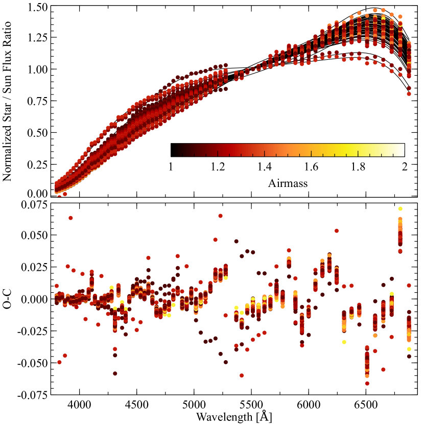
The resulting function is a combination of the systematic spectral difference between the star and the template, a general trend caused by the wavelength-dependent light loss due to either the telescope (e. g., mirror coating) or the instrument (e. g., CCD sensitivity curve), and small variations resulting from the difference between actual atmospheric refraction effect and the one predicted by the ADC for a given airmass.

5 The link between the CCF and the Equivalent Width

Determination of atmospheric parameters is based on the measurement of the equivalent width (EW) of spectral lines, and the numerical CCF is the direct transposition of spectral lines from wavelength to radial velocity space. We need to find an analytical formulation to compute the area subtended by the CCF starting from a set of EWs.

Spectral lines on the linear part of the curve of growth are usually approximated with a gaussian shape (Gray, 2005). An EW is obtained by measuring the depth of a line in the normalized spectrum $d$ (also known as the contrast of the line) and its full width half maximum $\Gamma$ in the wavelength space. Radial velocities of stars are always well below the relativistic limits (i. e., ${\rm RV}_{star}<1000$ km s^-1), so we can use the classical Doppler formula to transpose the EW in the radial velocity space, as in Equation (3).

$$\begin{split}{\rm EW}&=\frac{\sqrt{2\pi}}{2\sqrt{2\ln{2}}}d_{\lambda}\Gamma_{\lambda}\\ &=\frac{\sqrt{2\pi}}{2\sqrt{2\ln{2}}}\frac{\lambda_{0}}{c}d_{{\rm RV}}\Gamma_{{\rm RV}}\\ &=\frac{\lambda_{0}}{c}A_{{\rm CCF}}\end{split}$$ (3)

The normalized area $A_{{\rm CCF}}$ subtended by the CCF is equivalent to the EW of Equation (3) only when a single line is considered. Following Pepe et al. (2002), the observed CCF is obtained by coadding the individual CCFs from each line in the mask, without a prior normalization for their respective continuum. Consequently the corresponding area $A_{{\rm CCF}}$ is given by the sum of the areas of each spectral line $i$ in the CCF mask weighted by their continuum levels in the RV space. The value of the continuum level at the center of the CCF (i. e., ${\rm RV}=0$) for a generic line $i$ is obtained by applying the definition of the CCF to the continuum function $c(\lambda)$ at the wavelength $\lambda_{i}$ corresponding to the center of the spectral line, with $\delta^{i}_{\lambda}$ being the size of the bin used to compute the CCF, as in Equation (4).

$$c^{i}_{{\rm CCF}}(0)=\int_{\lambda_{i}-\delta^{i}_{\lambda}/2}^{\lambda_{i}+\delta^{i}_{\lambda}/2}c(\lambda)d\lambda\simeq\delta_{\lambda}c(\lambda_{i})$$ (4)

In a generic case it would be difficult to obtain the integrand from Equation (4). In practice, $\delta_{\lambda}$ is always chosen to be very small compared to the instrumental FWHM, so we can approximate $c(\lambda)$ as constant between the integration limits.

Using Equation (2) from Section 3, the expected CCF area as a function of the EWs of the spectral lines in the CCF mask can be determined (Equation 5).

$$\begin{split}A_{{\rm CCF}}&=\frac{\sum_{i}\delta^{i}_{\lambda}c(\lambda_{i})A_{i}}{c_{{\rm CCF}}(0)}\\ &=\frac{1}{c_{{\rm CCF}}(0)}\sum_{i}{\frac{\delta^{i}_{\lambda}mc_{t}(\lambda_{i})}{a(\lambda_{i})}A_{i}}\\ &=\frac{1}{c_{{\rm CCF}}(0)}\sum_{i}{\frac{\delta^{i}_{\lambda}mc_{t}(\lambda_{i})}{a(\lambda_{i})}\frac{\lambda_{i}}{c}{\rm EW}_{i}}\end{split}$$ (5)

All the variables in the right side of Equation (5) are known a priori ($c_{t}$, $\delta^{i}_{\lambda}$) or can be obtained by the observations themselves ($m$, $a$, $c_{{\rm CCF}}(0)$ using the sides of the CCF function), while the EW for each line $i$ in the CCF mask can be computed with a spectrum synthesis code. This result allows the determination of the expected CCF area as a function of the atmospheric parameters and the creation of a synthetic calibration.

6 Characteristic of the sample of stars

bf It is essential to have a calibration sample of stars that widely span the range in the stellar parameters that we want to calibrate. At our disposal we have $1111$ stars from several HARPS long-term programs (Mayor et al., 2003; Lo Curto et al., 2010; Santos et al., 2011). Since these stars are the targets of extensive exoplanet search surveys, a large number of exposures have been collected during several years of HARPS operations: this allows us to use the same stars as calibrators when considering the coadded, high SNR spectrum, and as test case when a single low SNR spectrum is under study.

Figure 2: The stellar atmosphere parameters of the calibration sample, derived by Adibekyan et al. (2012) using high SNR spectra. Except for $\xi_{\rm t}$, no trend between atmosphere parameters is present.

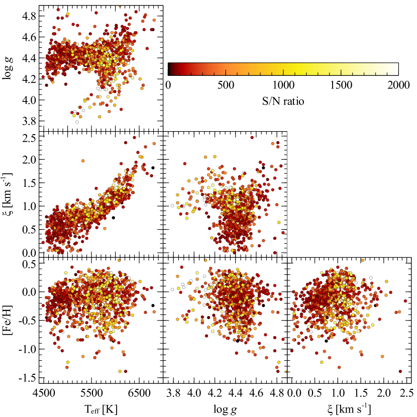
Stellar atmosphere parameters have been derived by Adibekyan et al. (2012) from co-added spectra using classical EW analysis. They employed empirical transition probabilities using Solar spectra as reference, thus making their analysis differential with respect to the Sun. The automatic continuum determination and EW  measurements performed with ARES (Sousa et al., 2007), ensure a high degree of homogeneity in the parameters derived for this sample. The distribution of the atmosphere parameters are displayed in Figure 2: the sample contains only dwarf stars with $\overline{\mbox{log\,{\it g}}}\simeq 4.4$, with a few exceptions. The targets span a wide range in $T_{\rm eff}$  and [Fe/H] without any correlation between the two parameters. A clear trend of micro-turbulence $\xi_{\rm t}$ with effective temperature is clearly visible. Since this relationship is well known and has been studied in the past (see for example the calibration of Tsantaki et al. 2013) we will not use the CCFs to derive this parameter. The quoted errors are $\sigma_{\textrm{$T_{\rm eff}$}}=30~{}$ K, $\sigma_{\textrm{\mbox{log\,{\it g}}}}=0.06~{}\textrm{dex}$ and $\sigma_{\textrm{\mbox{[{\rm Fe}/{\rm H}]}}}=0.03~{}\textrm{dex}$ on average. These uncertainties are internal of the method and do not include systematic source of errors such as the use of a specific set of stellar atmosphere models or departure from local thermodynamic equilibrium (LTE).

7 Line selection for the CCF masks

The HARPS Data Reduction Software (DRS) automatically determines an overall CCF and its parameters (central RV, FWHM and contrast) at the end of each exposure using one of the CCF masks provided by the DRS. Each mask contains several thousands of lines chosen among several chemical elements and ionization states and weighted according to the amount of radial velocity information they carry. For example, deep and sharp lines have larger weights simply because their RVs are easier to measure (Pepe et al., 2002). Three CCF masks are available, based on synthetic spectra of G2, K5 and M2 dwarf stars, in order to take into account the variation of line depths and flux distribution with the spectral type of the star. Since every line carries information on the radial velocity shift of the star regardless its chemical origin, and the principal goal of the instrument is to measure the differential shift of the star to a precision better than $1\textrm{m}/\textrm{s}$, all the available unsaturated lines are included in each mask in order to increase the SNR of the CCF.

In this work we are pursuing a different goal: to determine a correspondence between the characteristics of the CCF and the atmosphere parameters of the stars. For our purposes, significant noise can be added to the derived relationships by inclusion of lines with unknown atomic parameters or from chemical elements that can have large star-to-star abundance variations. We must make a more stringent selection of the lines included in the CCF mask in order to preserve the relationship between photospheric parameters and CCF characteristics without sacrificing excessively the SNR of the CCF.

To select a good sample of lines for our mask, we started with the list from Malavolta et al. (2016). This list includes 498 atomic line parameters from Sousa et al. (2011), which is in turn an extension of the iron line list from Sousa et al. (2007), and several chemical elements from Neves et al. (2009). Transition probabilities log gf have been updated to match the Solar EWs with the elemental abundances of Asplund et al. (2009). Our results will be then differential with respect to the Sun.

We briefly describe the procedure followed to derive the line list. The initial line list, along with the atomic parameters (including an initial estimate of the oscillator strengths) is taken from the VALD4 online database (Piskunov et al. 1995, Kupka et al. 2000) using the solar stellar parameters as input ($\textrm{$T_{\rm eff}$}=5777$ K, $\textrm{\mbox{log\,{\it g}}}=4.44$, $\xi=1.0$ km s^-1) in the spectral region from 4500 Å  to 6910 Å. The following criteria are followed:

• Lines must not be strongly blended in the Kurucz Solar Flux Atlas (Kurucz 2005 and references therein).

• Lines must not be too weak ($\textrm{EW}<5\,m$Å) or too strong ($\textrm{EW}>200\,m$Å)

• Lines must not reside in the wings of strong lines (e. g.H$\alpha$, H$\beta$ and MgI lines)

• EWs measured in the Kurucz Solar Flux Atlas and in the solar reflected light spectrum of the Ceres asteroid (obtained with HARPS) must agree within 10%.

• EWs of the lines can be appropriately measured using the ARES program (Sousa et al., 2007).

Finally empirical oscillator strengths are obtained through an inverse analysis with the ewfind driver of the LTE Spectral Synthesis code MOOG (Sneden, 1973) and the measured EWs from the solar spectrum, assuming for the Sun the parameters listed in Santos, Israelian & Mayor (2004).

The provided wavelengths are used as input positions by the ARES program to perform a Gaussian fit of the spectral lines in order to derive their EWs. However these wavelengths lack the required precision to be directly used in a cross-correlation mask, i. e., spectral lines are provided with a precision of $0.01$ Å, corresponding to a potential misplacement of the CCF of $0.545$ km s^-1 at $5500$ Å. We re-determined the central wavelengths of the lines by performing a multi-gaussian fit of each spectral line in the list on several solar spectra observed with HARPS. The new values are already included in Table 1.

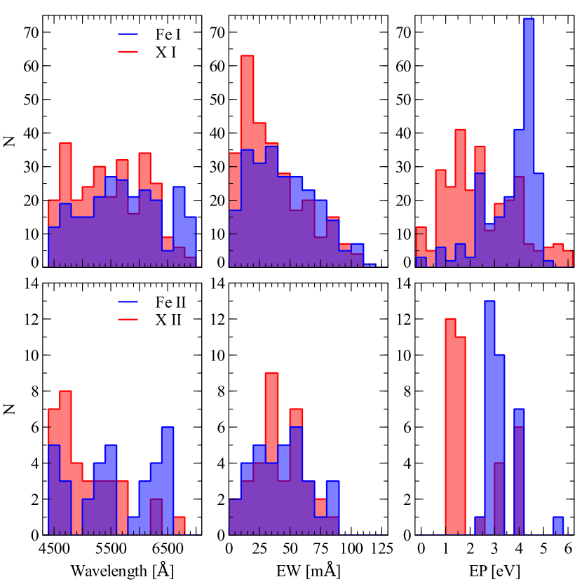
In Figure 3 the distributions of the selected lines versus the basic atomic line parameters are displayed. The selected lines are homogeneously distributed in wavelength and cover a good range in excitation potential (EP) and equivalent width as measured in the solar spectrum.

Figure 3: Distribution of selected neutral lines (upper panels) and ionized lines (lower panels) of Fe (blue histograms) and other “X” elements according to their wavelength, equivalent width (EW) measured in the solar spectrum and excitation potential (EP). The blue and red histograms are plotted separately, leading to overlapping (purple) parts of the histograms.

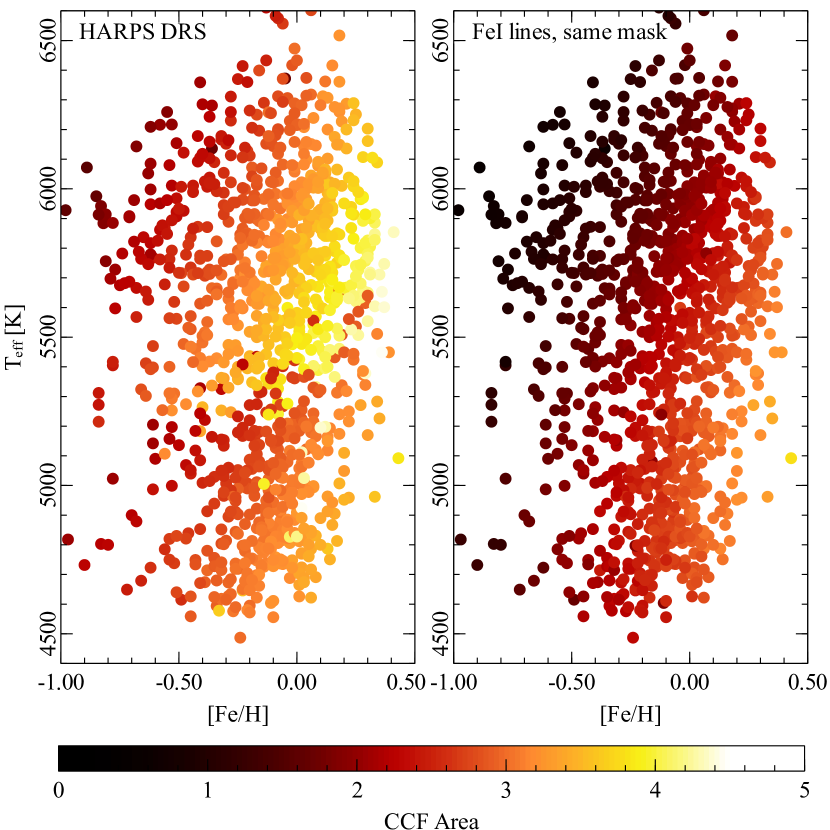
In Figure 4 the measured continuum-normalized area of the CCF determined by the HARPS pipeline (left panel) as a function of effective temperature and metallicity is compared with the CCF area obtained when only FeI lines are used (right panel), for the same set of stars in Figure 2. The jump in color in the left panel is due to the mask and flux correction template used for different spectral types, and it is the main reason why we cannot use the CCF information provided by the DRS pipeline. The area of the CCF varies smoothly when it is homogeneously derived for all the star in the sample. In both panels a degeneracy between temperature and metallicity is visible for a given CCF area. Every line depends on both the effective temperature of the photosphere and the abundance of the chemical element that is producing the line, and this behavior is conserved when the lines are co-added into a CCF. It is clear then that a single CCF area is not enough to constrain both metallicity and temperature if available. This is true regardless of the binary mask used for the CCF construction.

Figure 4: In the left panel, the CCF Area in function as determined by the HARPS DRS in the $T_{\rm eff}$- [Fe/H] plane; the jump in the area values is due to the different mask and spectral template used by the DRS for a given star. In the right panel, the area of the CCF as a function of the atmospheric parameters when using only FeI lines. In both panel, it is evident a degeneracy between $T_{\rm eff}$ and [Fe/H] for a given CCF area.

Fortunately, spectral lines react to temperature changes in different ways according to their atomic parameters. In classical stellar atmospheric parameters determination, a key parameter when determining the effective temperature of the star is the excitation potential (EP), i. e., the energy required to excite an atom to a given state from the ground state.

The presence of a trend between the abundances of individual Fe I lines (directly derived from their EWs) and the excitation potential is a clear sign of an incorrect $T_{\rm eff}$ assumed for the stellar model. The relationship between temperature and theoretical equivalent widths for lines with different excitation potentials is demonstrated with several examples in Figure 5. For each value of the effective temperature the EWs have been determined using a Kurucz model atmosphere with $\mbox{log\,{\it g}}=4.44$, $\mbox{$\xi_{\rm t}$}=1.0$ km s^-1 and $\mbox{[{\rm Fe}/{\rm H}]}=0.00$ using the ewfind driver of MOOG. Calculations have been performed for three neutral Fe lines and a ionized one. Helpful analytical expressions for EW curves as functions of temperature, excitation and ionization potentials are derived in Gray (2005).

Figure 5: Theoretical EWs curve for Iron lines with different excitation potentials and ionization state as a function of the effective temperature. Values have been calculated using Kurucz atmosphere models with log g, $\xi_{\rm t}$, and [Fe/H] fixed at the Solar values.

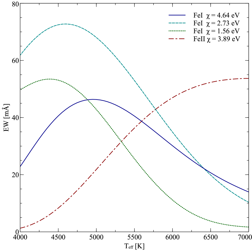
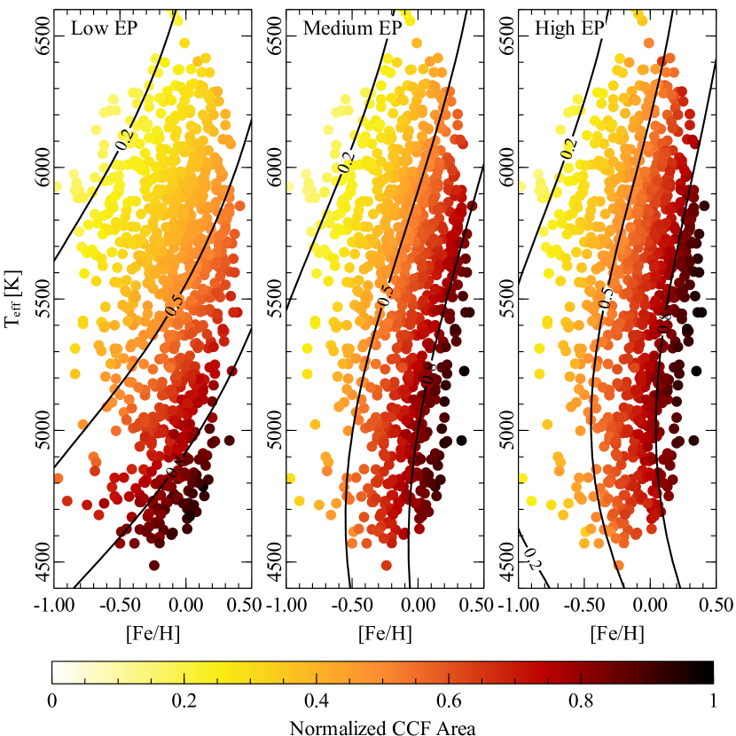
We can take advantage of the fact that at a given temperature the EW  curve of each line has a different slope, depending on its excitation potential, to create CCF masks whose associated areas have different gradients in the temperature-metallicity plane of Figure 4. We split our original linelist into three CCF masks:

(i) a mask with low excitation potential lines, comprising 243 lines with $\mbox{EP}<3.0$ eV ; (ii) a mask with 94 intermediate EP lines ($3.0<\mbox{EP}<4.0$ eV); (iii) a mask with 183 high excitation potential lines ($\mbox{EP}>4.0$ eV)

The list of spectral lines used in this work, their atomic parameters, and their mask membership are given in Table 1. The values obtained with these three mask will be identified respectively by the symbols $A_{low}$, $A_{med}$ and $A_{high}$ .

Table 1: Chemical elements, atomic parameters, solar EW from Adibekyan et al. (2012), contrast value of the spectral line as observed in the Solar spectra, and mask membership for all the spectral lines used in this work. Only a sample is given here, the full table will be available in the online version of the paper.

Chemical species	Wavelength [Å]	EP	log gf	$EW_{sun}$	Contrast	Maska
FeI	4554.462	2.870	-2.752	42.6	0.350	L
FeI	4561.413	2.760	-2.879	40.0	0.368	L
FeI	4574.722	2.280	-2.823	63.8	0.621	L
…	…	…	…	…	…	…

• L: low EP lines; M: intermediate EP lines; H: high EP lines; I: ionized lines.

In Figure 6 we can see that the iso-areas lines have different slopes for each mask, with stronger slope variations for cooler stars. As a result, a given combination of CCF areas will identify an unique point in the temperature-metallicity plane, i. e.only a single $($$T_{\rm eff}$,[Fe/H]$)$ pair can match the observed CCF Area, thus breaking the $T_{\rm eff}$- [Fe/H] degeneracy.

Figure 6: CCF areas as a function of temperature and metallicity, using the three masks defined in Section 7. Areas have been normalized to the maximum value of each mask for illustrative purpose only. Iso-area lines with values 0.2, 0.5 and 0.8 have been drawn to highlight the behaviour of the CCF areas derived with different masks.

8 Modeling the Temperature-Metallicity plane

In the temperature range of FGK dwarf stars most of the elements are in their first ionization stage, so weak lines formed by neutral elements are insensitive to pressure changes (Gray, 2005). In the previous section we described CCF masks composed of neutral-species transitions, with which we can derive an empirical calibration for $T_{\rm eff}$ and [Fe/H] which is suitable for dwarf stars (log g $\simeq 4.4\pm 0.3\,\textrm{dex}$) without requiring a precise knowledge of stellar gravity.

The easiest way to determine $T_{\rm eff}$ and [Fe/H] from the available CCF areas is to calibrate the two parameters as functions of the available CCF Area from high SNR spectra:

$$\textrm{$T_{\rm eff}$}=f_{1}(A_{\textrm{low}},A_{\textrm{med}},A_{\textrm{high}})$$ (6)

$$\textrm{\mbox{[{\rm Fe}/{\rm H}]}}=f_{2}(A_{\textrm{low}},A_{\textrm{med}},A_{\textrm{high}})$$ (7)

The two functions $f_{1}$ and $f_{2}$ can be represented in any form, i. e., either an analytical function or a list of tabulated values to be interpolated.

The coefficients of the functions are determined through Least Squares minimization using as input data $T_{\rm eff}$ and [Fe/H] from literature, and the CCF areas of the three masks measured on high SNR spectra.

The internal precision of the calibration is tested determining $T_{\rm eff}$ and [Fe/H] from the same area values used to determine the function coefficients. Figure 7 and Figure 8 show the difference between the stellar parameters used to calibrate Equations (6) and (7) as a function of the measured CCF areas, and the value returned by these functions when the same area values are given as input.

After exploring several possibilities, we decided to model $f_{1}$ and $f_{2}$ with three-dimensional Chebyshev polynomial functions of the first kind of order $6x6x6$. The Chebyshev polynomials are defined in the range $[-1,1]$, so the mid-points $A^{\textrm{mean}}$ and range $A^{\textrm{range}}$ for each variable must be chosen a priori. The variable transformation is defined by Equation (8).

$$A^{\prime}=(A^{\textrm{measured}}-A^{\textrm{mean}})/A^{\textrm{range}}$$ (8)

Figure 7: The internal precision of temperature determination using our technique is shown by taking the difference between the values used to determine $T_{\rm eff}$ as a function of CCF areas, and the values returned by the calibrated function Equation (6) for the same CCF areas. Blue lines show the precision of EWmeasurements, i. e., the values used to calibrate the function, red lines show the $1-\sigma$ precision of our calibration.

Figure 8: As in Figure 7, but for metallicity

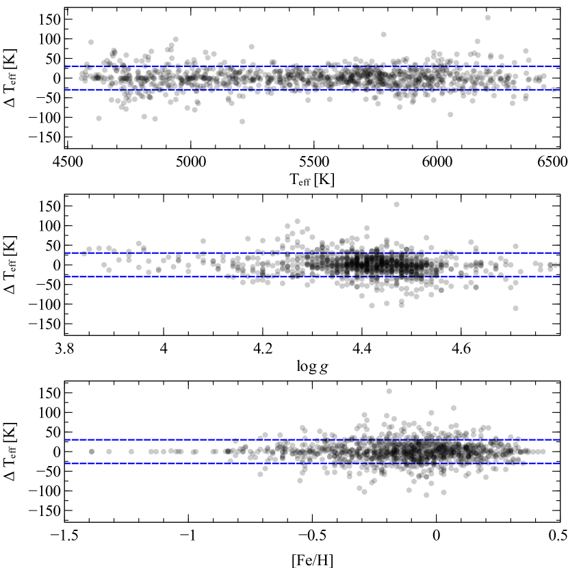
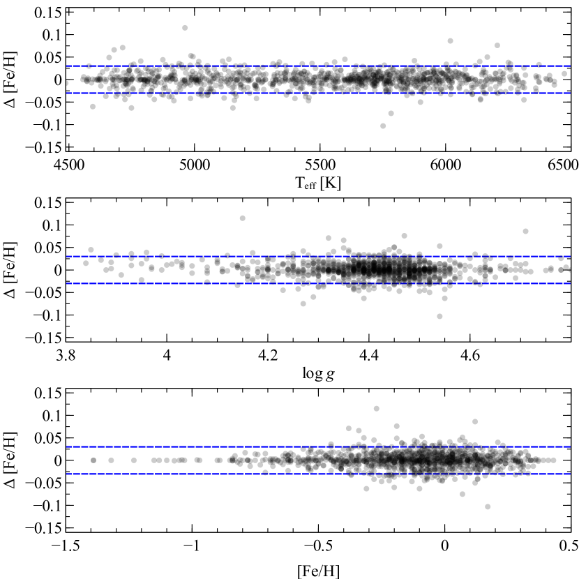
This choice led to an internal precision comparable with the spectroscopic formal error of the atmospheric parameters, and the absence of any systematic trend in the residuals. We obtained $\sigma_{\textrm{$T_{\rm eff}$}}=22$ K and $\sigma_{\textrm{\mbox{[{\rm Fe}/{\rm H}]}}}=0.02~{}\textrm{dex}$, against a reported precision of $\sigma_{\textrm{$T_{\rm eff}$}}=30$ K and $\sigma_{\textrm{\mbox{[{\rm Fe}/{\rm H}]}}}=0.03~{}\textrm{dex}$ from EW determination.

Once the coefficients of $f_{1}$ and $f_{2}$ have been determined, the only parameters required for $T_{\rm eff}$ and [Fe/H] determination are:

• the three line-lists in Tables 1;

• the coefficients of the Functions (6) and (7);

• the two parameters for each variables needed for Equation (8);

The CCFs must be computed with the same technique as described in Section 2; since the areas are normalized to the continuum level, the size of the bin in the mask is not relevant. Flux correction plays a major role, since it is changing the weights of single lines when assembling the CCF, and it should be performed as described in Section 4. Note that the general trend of stellar flux correction shown in Figure 1 is due to the technical characteristics of the telescope and spectrograph, and can be determined a priori. However, as a consequence the derived photospheric parameters will be affected by a larger uncertainties for not correcting night-by-night deviations from the general flux shape.

Generally speaking, the CCFs of the calibration sample and the CCF of a star with unknown parameters must be computed following the same algorithm, to ensure a correct determination of the stellar parameters.

9 Calibration of gravity

In principle, all the lines are sensitive to pressure changes: with increasing density, a larger number of absorbers per volume is available and the atomic lines are stronger. For cool stars however the strengths of neutral lines of most elements do not depend much on gravity, as discussed by Gray (2005) (see again Figures 7 and Figure 8).

On the other hand, lines arising from the ionized species of most elements are often very dependent on gravity. The rate of ionization of atoms depends on temperature, but the recombination rate is a function of temperature and gravity (Saha equation): recombination reduces the number of ionized atoms and it is faster with increasing pressure (gravity), thus lines from the most ionized states are very sensitive to this parameters.

In classical EW analyses, an initial guess at gravity is made to determine $T_{\rm eff}$ and [Fe/H] from neutral iron lines. Using the new determinations of the two parameters, the gravity estimate is improved by imposing ionization equilibrium of iron, i. e., the abundance derived from FeII lines must match that from FeI lines. The two steps are repeated until the three parameters converge.

We can proceed in a similar fashion to calibrate log g as a function of CCF area. Following the approach in Section 7 and Section 8, we define a CCF mask including isolated, unsaturated ionized lines for several elements, taken from Sousa et al. (2010) and Neves et al. (2009) and listed in Table 1 (identified with the mask flag I).

We firstly attempted to calibrate gravity as a function of the three CCF areas from neutral lines plus the CCF area using ionized lines, as done with $T_{\rm eff}$ and [Fe/H], but the coverage in gravity of our sample was not sufficient to derive a direct calibration of log g, not even when $T_{\rm eff}$ and [Fe/H] were externally provided. Keeping in mind that the CCF area from the ionized lines mask is also a function of temperature and metallicity, we followed this strategy to calibrate log g as a function of $A_{CCF}^{\star}$:

1. For each star, the CCF area using the ionized line mask $A_{CCF}^{\star}$ is measured.

2. For each star, the expected CCF area from EWs $A_{{\rm EW}}^{\star}$ is determined using Equation (5) and the atmospheric stellar parameters from literature;

3. The correction factor $F_{C}=A_{\textrm{{\rm CCF}}}^{\star}/A_{\textrm{{\rm EW}}}^{\star}$ is determined using stars with $\textrm{\mbox{log\,{\it g}}}=4.4\pm 0.1$ and modeled with a 2D Chebyshev polynomial function of the first kind (order $2\times 2$) as a function of temperature and metallicity (Figure 9).

4. For each star, $A_{\textrm{{\rm EW}}}^{\textrm{\mbox{log\,{\it g}}}}$ is evaluated for a grid of log g  values in the range $[3.6,4.9]$ and step 0.1 dex, as in step (ii).

5. $A_{\textrm{{\rm EW}}}^{\textrm{\mbox{log\,{\it g}}}}$ are rescaled to the expected $A_{CCF}^{\textrm{\mbox{log\,{\it g}}}}$ values by using the function $F_{c}$ determined in step (iii).

6. For each log g  grid point, $A_{CCF}^{\textrm{\mbox{log\,{\it g}}}}$ is modeled as a function of $T_{\rm eff}$  and [Fe/H]  with a 2D Chebyshev polynomial (order $3\times 3$).

Figure 9: The correction factor $F_{C}(\textrm{$T_{\rm eff}$},\textrm{\mbox{[{\rm Fe}/{\rm H}]}})$ required to rescale the synthesis-derived CCF areas to the actual values measured in stars. Only stars with $4.3<\mbox{log\,{\it g}}<4.5$ have been included here. The resulting 2D Chebyshev polynomial fit is represented by the solid lines.

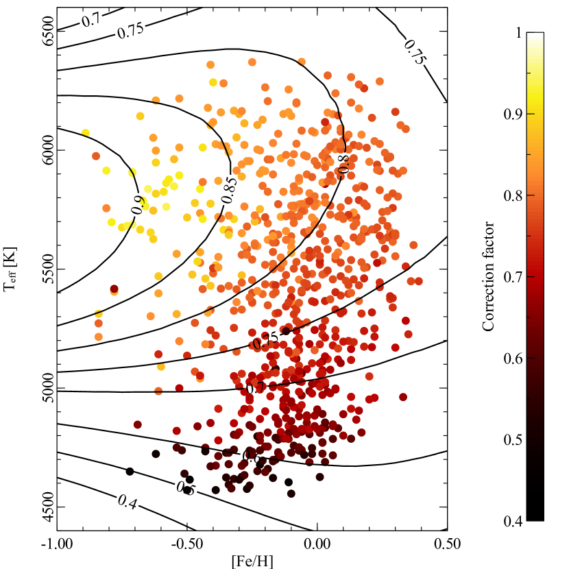
The difference between synthetic and observed values for the CCF areas, modeled with the function $F_{c}$, is mainly due to the influence of nearby spectral lines which lower the observed CCF continuum but are not taken in account in Equation (5). This explains why the ratio $F_{C}$ is systematically lower than unity and gets lower at cooler temperatures, where spectral lines grow in depth.

EWs are calculated using the ewfind driver of MOOG. For the continuum determination, we decided to use the synthetic flux-calibrated stellar spectrum closest to the Sun from the Coelho et al. (2005) stellar library, which has $\textrm{$T_{\rm eff}$}=5750$ K, $\textrm{\mbox{log\,{\it g}}}=4.5~{}\textrm{dex}$, $\textrm{\mbox{[{\rm Fe}/{\rm H}]}}=0.0~{}\textrm{dex}$. The systematic flux variations introduced by using a single synthesis as reference for a broad range of spectral types is taken automatically into account in the calibration of $F_{C}(\textrm{$T_{\rm eff}$},\textrm{\mbox{[{\rm Fe}/{\rm H}]}})$.

Following the approach described above, to determine the stellar gravity $T_{\rm eff}$  and [Fe/H]  must be provided as input, using for example the values derived in Section 8). The values of $A_{\textrm{{\rm CCF}}}^{\textrm{\mbox{log\,{\it g}}}}$ computed at $T_{\rm eff}$  and [Fe/H]  are then retrieved for each point of the log g  grid and interpolated, with log g as a function of $A_{\textrm{{\rm CCF}}}$. Finally the gravity value is determined by using the $A^{\star}_{{\rm CCF}}$ measured from the spectrum with the ionized lines mask.

As done for $T_{\rm eff}$  and [Fe/H]  in Section 8, we test the internal precision of the calibration by comparing the derived log g’s for the calibrators and the log g${}_{\textrm{{\rm EW}}}$ values from the literature. In the top panel of Figure 10, the difference between these two values $\Delta\textrm{\mbox{log\,{\it g}}}$ is plotted against the gravity from literature. A clear trend with the gravity of the star is present, possibly caused by our approach in determining the correction factor $F_{C}(\textrm{$T_{\rm eff}$},\textrm{\mbox{[{\rm Fe}/{\rm H}]}})$, which appears to be function of log g  as well. Since we do not have enough data to calibrate the correction factor as a function of gravity, a different approach has to be taken.

Figure 10: Upper panel: The difference between CCF-derived and EW-derived gravity is plotted against gravity from literature. Middle panel: the difference between the CCF area determined using the ionized lines mask and the expected synthetic value is plotted as a function of the gravity derived with the CCF approach. A quadratic fit is performed to model the systematic trend. Lower panel: The difference between the value obtained from the CCF calibration after correcting for the systematic trend and the one from EW  analysis is plotted against literature gravity.

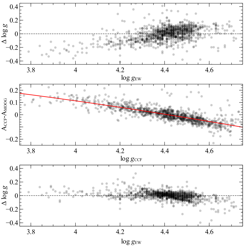
In the middle panel of Figure 10 the difference between the CCF area determined using the ionized lines mask and the expected synthetic value is plotted as a function of the gravity derived from the CCF area. The red line represents a quadratic fit to the overall trend. The scatter around this line is $\sigma{\Delta A}=0.026$, which is around $1-2\%$ of the average value of the CCF area. We decided to model such difference as a function of the derived gravity instead of the literature gravity so that we can apply this correction even for star without any a priori knowledge of the gravity. Following this approach, an approximation of gravity is firstly determined using the measured CCF area, the area correction value is determined using the derived value of gravity and added to the previously measured CCF area, and then this corrected value is used to get the final estimate of gravity. The bottom panel of Figure 10 is a replica of the upper panel, with the CCF-derived gravity now determined after applying the model introduced in the middle panel.

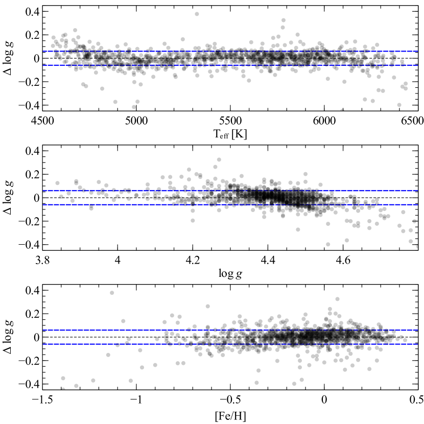
Results for calibrators stars are presented in Figure 11 in a similar fashion as done for temperature and metallicity. The dispersion in the residual distribution is of the same order of the average formal error ($\sigma_{\mbox{log\,{\it g}}}=0.076\,\textrm{dex}$ versus $<\sigma>_{\mbox{log\,{\it g}}}=0.06\,\textrm{dex}$), although a residual trend with temperature and metallicity is still present and at higher values of gravity and lower temperatures the calibration seems to be less reliable. While a more complex approach than the one presented in this section should be followed to correct for the systematic deviations in Figure 10, we note that the amplitude of the residual trend is smaller than the average error of the calibration stars (blue dashed lines in the Figure), meaning that no real improvement of the results would be obtained. Therefore we preferred to rely on our simpler but more robust approach.

Figure 11: As in Figure 7, but for gravity

10 Atmospheric parameters as a function of SNR

We applied the technique described in the previous sections to each individual exposure obtained with HARPS within the planet-search survey described in Section 6, and compared the outcome with the EW-based atmospheric parameters obtained after stacking together the exposures. These observations have been gathered in different weather condition and sometimes with different integration times, but usually for a given star the observations are clustered around the SNR  expected for average observing conditions. The number of observations varies largely from star to star, from a few observations to several hundreds, depending on the specific goal for that target (e. g., characterize its activity rather than discovering new planets). We analyzed a total of $\simeq 56000$ spectra, but we decided to retain for each star a maximum of 10 randomly selected determinations of the atmospheric parameters to better represent the dispersion of the parameters as a function of SNR, i. e., to avoid biasing the plot towards stars with many observations.

Temperature and metallicity are derived using the direct calibration introduced in Section 8; gravity is then derived as described in Section 9, using the obtained stellar parameters as input. It is important to notice that these calibrations, although very precise, are reliable only in the range of parameters used to derive the functions (6) and (7).

Figure 12: Difference between the CCF-derived atmospheric parameters for individual HARPS spectra and the EW-derived parameters from high-SNR  stacked spectra, as a function of the SNR. Temperature and metallicity have been derived using the direct calibration, while for gravity we used the former two parameters as input. Cyan points represent the $1\sigma$ dispersion for several bins of SNR. The red line is the inverse square root law fit of the dispersion as a function of the SNR. Blue dashed lines represent the average error from EW-derived parameters.

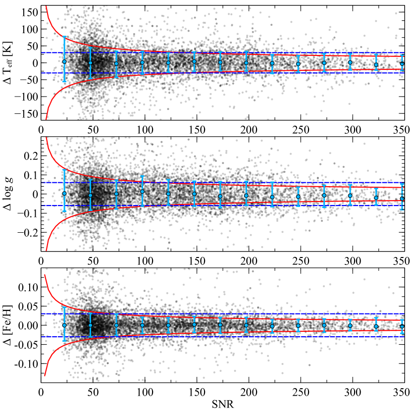
To determine the precision as a function of SNR, the $\sigma$ of the distribution of the difference has been computed for several bins of SNR. At low SNR a simple inverse square-root law of SNR  provides a very good fit of the points, proving that our measurements are photon-limited. For $\textrm{\mbox{SNR}}=50$ we have a precision of $\sigma_{\textrm{$T_{\rm eff}$}}=50$ K, $\sigma_{\textrm{\mbox{log\,{\it g}}}}=0.09~{}\textrm{dex}$ and $\sigma_{\textrm{\mbox{[{\rm Fe}/{\rm H}]}}}=0.035~{}\textrm{dex}$, while the accuracy of the technique is provided by the accuracy of the atmosphere parameters of the calibrators. The precision of our technique is limited by the goodness of the calibration at a SNR  between 100 and 150, so for SNR  similar or greater than these values the average error from EW  analysis should be considered as an estimate for the associated errors.

11 Discussion

We have presented a new technique to quickly determine reliable stellar atmosphere parameters for FGK Main Sequence stars using several CCFs specifically built to be more sensitive to a given atmosphere parameter respect to the others. Our approach relies on a set of high-resolution, high SNR  stars already classified spectroscopically, which defines the limit on the accuracy of our technique.

We have developed this approach with two goals in mind. The first goal is to enable the spectroscopic classification of stellar objects at observing time, a few seconds after the end of the exposure, with a precise tool that is quick and easy to use at the same time. This tool can be extremely useful when performing time series of poorly characterized target, e. g., follow-up of faint planet-host candidates, to exclude stars that do not match a criteria selection (e. g., stars that are not solar-type stars) after one or two observations with a considerable optimization of telescope time. The second goal is to determine atmospheric parameters of faint objects observed at very low SNR  with high-resolution spectroscopy, when an equivalent width analysis is still not feasible even after co-addition of all the available spectra.

To find the relationship between CCFs parameters and photosphere parameters we have used a dataset of high-resolution, high SNR  spectra of 1111 stars with accurate parameters derived using equivalent widths from literature. The spectrum of each star is actually the result of a co-addition of several spectra at lower SNR, since these data have been gathered for exoplanet search. The lower SNR  spectra have allowed us to understand the effective precision of our technique on real data.

Two different calibrations have been presented. The first is purely empirical and it provides temperature and metallicity from the observed CCF areas for stars with parameters in the ranges $\textrm{$T_{\rm eff}$}\simeq[4500,6500]$ K, $\textrm{\mbox{log\,{\it g}}}\simeq[4.2,4.8]$ and $\textrm{\mbox{[{\rm Fe}/{\rm H}]}}\simeq[-1.0,0.5]$ (solar-type and slightly evolved stars). We achieve a precision of $\sigma_{\textrm{$T_{\rm eff}$}}=50$ K and $\sigma_{\textrm{\mbox{[{\rm Fe}/{\rm H}]}}}=0.035~{}\textrm{dex}$ at $\textrm{\mbox{SNR}}=50$, with the precision being an inverse square-root law of SNR. The second calibration is based on the transformation of synthetic equivalent width in CCF areas and it allows the determination of gravity when temperature and metallicity are provided as input. For gravity we reach a precision of $\sigma_{\textrm{\mbox{log\,{\it g}}}}=0.09~{}\textrm{dex}$, with this value taking into account the errors in $T_{\rm eff}$ and [Fe/H] introduced by the empirical calibration. In both cases the precision for HARPS spectra with SNR $\gtrsim$ 100 and the overall accuracy are limited by the set of stars used as reference. Given the very high SNR of the calibration sample, better performance can be achieved by expanding the parameter space covered by the calibration stars, e. g., by including stars at lower metallicity, rather than increasing the number of observations of the stars already in the sample.

We have developed this open-source tool for HARPS and HARPS-N data and for FGK Main Sequence stars, but our approach can be easily extended to other instruments with similar or larger spectral range and similar resolution, or to other spectral range and stars with different characteristics (e. g., Red Giant Branch stars or M dwarfs) if a large sample of reference stars is available to calibrate the CCFs as a function of photospheric parameters. When either of the two cases above does not apply, we provide the mathematical formulation required to transform synthetic EWs to CCF areas. Our tool will allow an easy, quick and reliable characterization of candidate transiting planets from present and future transit surveys such as NGTS (Chazelas et al., 2012), TESS (Ricker et al., 2014) and PLATO (Rauer et al., 2014).

References

- Adibekyan et al. (2012) Adibekyan V. Z., Sousa S. G., Santos N. C., Delgado Mena E., González Hernández J. I., Israelian G., Mayor M., Khachatryan G., 2012, A&A, 545, 32
- Allende Prieto (2016) Allende Prieto C., 2016, Astronomische Nachrichten, 337, 837
- Asplund et al. (2009) Asplund M., Grevesse N., Sauval A. J., Scott P., 2009, ARA&A, 47, 481
- Baranne, Mayor & Poncet (1979) Baranne A., Mayor M., Poncet J. L., 1979, Vistas in Astronomy, 23, 279
- Baranne et al. (1996) Baranne A. et al., 1996, Astron Astrophys Sup, 119, 373
- Beers et al. (1999) Beers T. C., Rossi S., Norris J. E., Ryan S. G., Shefler T., 1999, AJ, 117, 981
- Chazelas et al. (2012) Chazelas B. et al., 2012, in Proc. SPIE, Vol. 8444, Ground-based and Airborne Telescopes IV, p. 84440E
- Coelho et al. (2005) Coelho P., Barbuy B., Meléndez J., Schiavon R. P., Castilho B. V., 2005, A&A, 443, 735
- De Medeiros et al. (2014) De Medeiros J. R., Alves S., Udry S., Andersen J., Nordström B., Mayor M., 2014, A&A, 561, A126
- Endl & Cochran (2016) Endl M., Cochran W. D., 2016, PASP, 128, 094502
- Gray (2005) Gray D. F., 2005, The Observation and Analysis of Stellar Photospheres
- Kupka et al. (2000) Kupka F. G., Ryabchikova T. A., Piskunov N. E., Stempels H. C., Weiss W. W., 2000, Baltic Astronomy, 9, 590
- Kurucz (2005) Kurucz R. L., 2005, Memorie della Societa Astronomica Italiana Supplementi, 8, 189
- Lo Curto et al. (2010) Lo Curto G. et al., 2010, A&A, 512, 48
- Majewski, APOGEE Team & APOGEE-2 Team (2016) Majewski S. R., APOGEE Team, APOGEE-2 Team, 2016, Astronomische Nachrichten, 337, 863
- Malavolta et al. (2016) Malavolta L. et al., 2016, A&A, 588, A118
- Malavolta et al. (2015) Malavolta L., Piotto G., Bedin L. R., Sneden C., Nascimbeni V., Sommariva V., 2015, MNRAS, 454, 2621
- Malavolta et al. (2014) Malavolta L., Sneden C., Piotto G., Milone A. P., Bedin L. R., Nascimbeni V., 2014, AJ, 147, 25
- Mayor et al. (2003) Mayor M. et al., 2003, The Messenger, 114, 20
- Mayor & Queloz (1995) Mayor M., Queloz D., 1995, Nature, 378, 355
- Neves et al. (2009) Neves V., Santos N. C., Sousa S. G., Correia A. C. M., Israelian G., 2009, A&A, 497, 563
- Pepe et al. (2002) Pepe F., Mayor M., Galland F., Naef D., Queloz D., Santos N. C., Udry S., Burnet M., 2002, A&A, 388, 632
- Piskunov et al. (1995) Piskunov N. E., Kupka F., Ryabchikova T. A., Weiss W. W., Jeffery C. S., 1995, Astron Astrophys Sup, 112, 525
- Ratnatunga & Freeman (1989) Ratnatunga K. U., Freeman K. C., 1989, ApJ, 339, 126
- Rauer et al. (2014) Rauer H. et al., 2014, Experimental Astronomy, 38, 249
- Ricker et al. (2014) Ricker G. R. et al., 2014, in Proc. SPIE, Vol. 9143, Space Telescopes and Instrumentation 2014: Optical, Infrared, and Millimeter Wave, p. 914320
- Santos, Israelian & Mayor (2004) Santos N. C., Israelian G., Mayor M., 2004, A&A, 415, 1153
- Santos et al. (2011) Santos N. C. et al., 2011, A&A, 526, 112
- Sneden (1973) Sneden C., 1973, Astrophysical Journal, 184, 839
- Sousa et al. (2010) Sousa S. G., Alapini A., Israelian G., Santos N. C., 2010, A&A, 512, A13
- Sousa et al. (2007) Sousa S. G., Santos N. C., Israelian G., Mayor M., Monteiro M. J. P. F. G., 2007, A&A, 469, 783
- Sousa et al. (2011) Sousa S. G., Santos N. C., Israelian G., Mayor M., Udry S., 2011, A&A, 533, A141
- Teixeira et al. (2016) Teixeira G. D. C., Sousa S. G., Tsantaki M., Monteiro M. J. P. F. G., Santos N. C., Israelian G., 2016, ArXiv e-prints
- Tsantaki et al. (2013) Tsantaki M., Sousa S. G., Adibekyan V. Z., Santos N. C., Mortier A., Israelian G., 2013, A&A, 555, A150
- Xiang et al. (2017) Xiang M.-S. et al., 2017, MNRAS, 464, 3657
- Yee, Petigura & von Braun (2017) Yee S. W., Petigura E. A., von Braun K., 2017, ArXiv e-prints
- Zucker et al. (2012) Zucker D. B., de Silva G., Freeman K., Bland-Hawthorn J., Hermes Team, 2012, in Astronomical Society of the Pacific Conference Series, Vol. 458, Galactic Archaeology: Near-Field Cosmology and the Formation of the Milky Way, Aoki W., Ishigaki M., Suda T., Tsujimoto T., Arimoto N., eds., p. 421