Implementing NLO DGLAP evolution in Parton Showers

Abstract

We present a parton shower which implements the DGLAP evolution of parton densities and fragmentation functions at next-to-leading order precision up to effects stemming from local four-momentum conservation. The Monte-Carlo simulation is based on including next-to-leading order collinear splitting functions in an existing parton shower and combining their soft enhanced contributions with the corresponding terms at leading order. Soft double counting is avoided by matching to the soft eikonal. Example results from two independent realizations of the algorithm, implemented in the two event generation frameworks P YTHIA and S HERPA , illustrate the improved precision of the new formalism.

I Introduction

Parton shower algorithms describing QCD and QED multiple radiation have been a central ingredient of simulation programs for particle physics experiments at the energy frontier Buckley et al. (2011). After their inception about three decades ago, where the focus was on QCD radiation in the final state Fox and Wolfram (1980), efficient algorithms for initial state radiation were developed Sjöstrand (1985), which amount to evolution back in “time” from the hard scattering to the incoming beam hadrons. The study of quantum interference effects in successive emissions led to the notion of QCD coherence in parton evolution Azimov et al. (1985a, b), and angular ordering was identified as a convenient scheme that incorporates such effects Webber (1984); Marchesini and Webber (1984, 1988). As an alternative scheme, the color dipole model Gustafson and Pettersson (1988); Lönnblad (1992) includes QCD coherence in a natural way. Matrix-element corrections have been investigated as a source of coherence Bengtsson and Sjöstrand (1987a, b).

After about a decade of work on matching Frixione and Webber (2002); Höche et al. (2012); Hamilton et al. (2013a, b); Höche et al. (2015, 2014) and merging Catani et al. (2001); Lönnblad (2002); Krauss (2002); Mangano et al. (2007); Alwall et al. (2008); Höche et al. (2009); Hamilton and Nason (2010); Höche et al. (2013); Plätzer (2013); Lönnblad and Prestel (2013a, b); Frederix and Frixione (2012) algorithms, the necessity of increased control over the parton shower for a more seamless combination with fixed-order calculations at higher orders triggered a resurgence of interest in improving parton-shower algorithms themselves. As a consequence, new parton showers Sjöstrand and Skands (2005); Schumann and Krauss (2008); Dinsdale et al. (2007); Winter and Krauss (2008); Giele et al. (2008); Plätzer and Gieseke (2011); Ritzmann et al. (2013); Höche and Prestel (2015), have been constructed that are based on ordering subsequent emissions in transverse momenta, and there were also new constructions with improved and generalized angular ordering parameters Gieseke et al. (2003). The possibility of including next-to-leading order corrections into parton showers was explored over three decades ago Kato and Munehisa (1987, 1989, 1991); Kato et al. (1992), and it was revisited recently in a different framework Hartgring et al. (2013); Li and Skands (2016). Next-to-leading order corrections to a single final-state gluon emission off a $q\bar{q}$ dipole have been presented in Hartgring et al. (2013) as a first higher-order extension of the antenna shower formalism. How this approach maps onto NLO DGLAP evolution was briefly addressed in Li and Skands (2016), which furthermore introduced final-state double-gluon radiation into this formalism. In addition to this, NLO splitting functions have been recomputed using a novel regularization scheme Jadach et al. (2011); Gituliar et al. (2014), with the aim to improve parton-shower simulations. The dependence of NLO matching terms on the parton-shower evolution variable has also been investigated Jadach et al. (2016).

This publication is dedicated to the construction of a parton shower that implements the next-to-leading order (NLO) DGLAP equations up to momentum conserving effects. We employ the non-flavor changing NLO splitting functions in the $\overline{\rm MS}$ scheme in their integrated form Curci et al. (1980); Furmanski and Petronzio (1980); Floratos et al. (1981a, b); Heinrich and Kunszt (1998); Ellis and Vogelsang , and we include the flavor-changing NLO splitting kernels fully differentially using the method presented in Höche and Prestel (2017). We identify the contribution to the NLO splitting functions which is already included in the leading-order (LO) realization of the parton-shower, and correspondingly subtract it from the NLO splitting function. This term is given by the two-loop cusp anomalous dimension, which is usually included at LO using the CMW scheme Catani et al. (1991). After its subtraction, the remaining splitting function is purely collinear, and no double-counting arises upon implementing it as a higher-order correction to the existing splitting kernels of the parton shower. However, the NLO parts of the splitting functions are negative in large parts of the phase space which presents a technical challenge. We overcome this problem through the weighting algorithm first proposed in Höche et al. (2010); Lönnblad (2012). Our approach can be considered as a first step towards a fully next-to-leading order accurate parton shower and acts as a baseline for further development. Future projects will need to address the leading-color approximation and the simulation of soft emissions beyond the leading order. The Monte-Carlo techniques developed here are expected to become useful in this context as well. A clear phenomenological benefit of the present implementation is that consistency between the parton shower and NLO PDF evolution is achieved for the very first time.

The outline of this paper is as follows. Section II introduces the parton-shower formalism at leading order and establishes the connection to the DGLAP equation in order to identify the correct treatment of the final-state Sudakov factor. Section III outlines the specific implementation in the D IRE parton showers Höche and Prestel (2015). First results and applications are presented in Sec. IV. Section V contains our conclusions.

II Extension of the parton-shower formalism

In this section we will highlight the correspondence between the parton shower formalism and the analytic structure of the DGLAP evolution equations Gribov and Lipatov (1972); *Dokshitzer:1977sg; *Altarelli:1977zs, on which the parton shower is based. We will thereby focus on the refinements needed in order to realize NLO accurate parton evolution. This includes the implementation of the complete set of splitting kernels at $\mathcal{O}(\alpha_{s}^{2})$, a subset of which are the flavor-changing kernels discussed in Höche and Prestel (2017). Another significant change concerns the implementation of symmetry factors. In the computation of the NLO splitting functions Curci et al. (1980); Furmanski and Petronzio (1980); Floratos et al. (1981a, b); Heinrich and Kunszt (1998); Ellis and Vogelsang , it is assumed that a certain final-state parton is identified, while the parton shower treats all particles democratically. If the full set of splitting functions – both at leading and at next-to-leading order – is implemented naively, the emission probability will thus be overestimated. At leading-order the problem can be solved by adding simple symmetry factors. At next-to-leading order the solution will be different, as the splitting functions include contributions from three-particle final states that have been integrated out. We will show in the following how this problem can be approached Höche and Prestel (2017).

II.1 Unconstrained evolution with identified final-states

The DGLAP equations are schematically identical for initial and final state. However, their implementation in parton-shower programs differs between the two, owing to the fact that Monte-Carlo simulations are typically performed for inclusive final states. The inclusive evolution equations for the fragmentation functions $D_{a}(x,Q^{2})$ for parton of type $a$ to fragment into a hadron read

$$\frac{{\rm d}\,xD_{a}(x,t)}{{\rm d}\ln t}=\sum_{b=q,g}\int_{0}^{1}{\rm d}\tau\int_{0}^{1}{\rm d}z\,\frac{\alpha_{s}}{2\pi}\big{[}zP_{ab}(z)\big{]}_{+}\,\tau D_{b}(\tau,t)\,\delta(x-\tau z)\;,$$ (1)

where the $P_{ab}$ are the unregularized DGLAP evolution kernels, and the plus prescription is defined to enforce the momentum and flavor sum rules:

$$\big{[}zP_{ab}(z)\big{]}_{+}=\lim\limits_{\varepsilon\to 0}\bigg{[}zP_{ab}(z)\,\Theta(1-z-\varepsilon)-\delta_{ab}\sum_{c\in\{q,g\}}\frac{\Theta(z-1+\varepsilon)}{\varepsilon}\int_{0}^{1-\varepsilon}{\rm d}\zeta\,\zeta\,P_{ac}(\zeta)\bigg{]}\;.$$ (2)

For finite $\varepsilon$, the endpoint subtraction in Eq. (2) can be interpreted as the approximate virtual plus unresolved real corrections, which are included in the parton shower because the Monte-Carlo algorithm naturally implements a unitarity constraint Jadach and Skrzypek (2004). The precise value of $\varepsilon$ in this case depends on the infrared cutoff on the evolution variable, and is determined by local four-momentum conservation in the parton branching process. For $0<\varepsilon\ll 1$, Eq. (1) changes to

$$\frac{1}{D_{a}(x,t)}\,\frac{{\rm d}D_{a}(x,t)}{{\rm d}\ln t}=-\sum_{c=q,g}\int_{0}^{1-\varepsilon}{\rm d}\zeta\,\zeta\,\frac{\alpha_{s}}{2\pi}P_{ac}(\zeta)\,+\sum_{b=q,g}\int_{x}^{1-\varepsilon}\frac{{\rm d}z}{z}\,\frac{\alpha_{s}}{2\pi}\,P_{ab}(z)\,\frac{D_{b}(x/z,t)}{D_{a}(x,t)}\;.$$ (3)

Using the Sudakov form factor

$$\Delta_{a}(t_{0},t)=\exp\bigg{\{}-\int_{t_{0}}^{t}\frac{{\rm d}\bar{t}}{\bar{t}}\sum_{c=q,g}\int_{0}^{1-\varepsilon}{\rm d}\zeta\,\zeta\,\frac{\alpha_{s}}{2\pi}P_{ac}(\zeta)\bigg{\}}$$ (4)

the generating function for splittings of parton $a$ is defined as

$$\mathcal{D}_{a}(x,t,\mu^{2})=D_{a}(x,t)\Delta_{a}(t,\mu^{2})\,.$$ (5)

Equation (3) can now be written in the simple form

$$\frac{{\rm d}\ln\mathcal{D}_{a}(x,t,\mu^{2})}{{\rm d}\ln t}=\sum_{b=q,g}\int_{x}^{1-\varepsilon}\frac{{\rm d}z}{z}\,\frac{\alpha_{s}}{2\pi}\,P_{ab}(z)\,\frac{D_{b}(x/z,t)}{D_{a}(x,t)}\;.$$ (6)

The generalization to an $n$-parton state, $\vec{a}=\{a_{1},\ldots,a_{n}\}$, with jets and incoming hadrons resolved at scale $t$ can be made in terms of parton distribution functions (PDFs) $f$, and fragmenting jet functions, $\mathcal{G}$ Procura and Stewart (2010); Jain et al. (2011). If we define the generating function for this state as $\mathcal{F}_{\vec{a}}(\vec{x},t,\mu^{2})$, we can formulate its evolution equation in terms of a sum of the right hand side of Eq. (6), where each term in the sum corresponds to a resolved jet in the final state or a hadron in the initial state. This equation can be solved using Markovian Monte-Carlo techniques in the form of a parton shower Buckley et al. (2011). In most cases, however, parton showers implement final-state branchings in unconstrained evolution, which means that final-state hadrons are not resolved. We can use Eq. (3) (which also applies to $\mathcal{G}$ Procura and Stewart (2010); Jain et al. (2011)), to write the corresponding differential decay probability for such an evolution as

$$\begin{split}\frac{{\rm d}}{{\rm d}\ln t}\ln\bigg{(}\frac{\mathcal{F}_{\vec{a}}(\vec{x},t,\mu^{2})}{\prod_{j\in\rm FS}\mathcal{G}_{a_{j}}(x_{j},t)}\bigg{)}=&\sum_{i\in{\rm IS}}\sum_{b=q,g}\int_{x_{i}}^{1-\varepsilon}\frac{{\rm d}z}{z}\,\frac{\alpha_{s}}{2\pi}\,P_{ba_{i}}(z)\,\frac{f_{b}(x_{i}/z,t)}{f_{a_{i}}(x_{i},t)}+\sum_{j\in{\rm FS}}\sum_{b=q,g}\int_{0}^{1-\varepsilon}{\rm d}z\,z\,\frac{\alpha_{s}}{2\pi}\,P_{a_{j}b}(z)\;.\end{split}$$ (7)

As highlighted in Jadach and Skrzypek (2004), it is necessary to use the Sudakov factor, Eq. (4), in final-state parton showers beyond the leading order. At the leading order, the factor $\zeta$ in Eq. (4) simply replaces the commonly used symmetry factor for $g\to g$ splitting and it also accounts for the proper counting of the number of active flavors. However, at the next-to-leading order it becomes an identifier for the parton that undergoes evolution, which is essential in order to obtain the correct anomalous dimensions upon integration of the NLO DGLAP evolution kernels. We will thus define the final-state Sudakov factor in our implementation according to Eq. (4).

II.2 Splitting functions

The crucial ingredient of NLO DGLAP evolution are the $\mathcal{O}(\alpha_{s}^{2})$ corrections to the evolution kernels. These corrections depend on the scheme in which PDFs and fragmentation functions are renormalized. We will work in the $\overline{\rm MS}$ scheme, which allows us to use the results of Curci et al. (1980). Technical challenges in the implementation of the splitting functions in the parton shower include the overlap with the CMW scheme for setting the renormalization scale commonly used in leading-order parton showers Catani et al. (1991) as well as the fact that the evolution kernels are negative in large parts of the accessible phase space. We will discuss these problems in a general context in the following and give more details on the implementation in the Dire parton showers in Sec. III.

At $\mathcal{O}(\alpha_{s})$, the unregularized DGLAP splitting functions are

$$\begin{split}P_{qq}^{(0)}(z)=&\;C_{F}\bigg{[}\frac{1+z^{2}}{1-z}\bigg{]}\;,\qquad P_{gq}^{(0)}(z)=T_{R}\Big{[}1-2z(1-z)\Big{]}\;,\\ P_{gg}^{(0)}(z)=&\;2C_{A}\bigg{[}\frac{z}{1-z}+\frac{1-z}{z}+z(1-z)\bigg{]}\;.\end{split}$$ (8)

At $\mathcal{O}(\alpha_{s}^{2})$, the quark splitting functions are typically written in terms of singlet (S) and non-singlet (V) components as

$$\begin{split}P_{qq}^{(1)}(z)=&\;p_{qq}^{V(1)}(z)+p_{qq}^{S(1)}(z)\;,\qquad&P_{q\bar{q}}^{(1)}(z)=&\;p_{q\bar{q}}^{V(1)}(z)+p_{qq}^{S(1)}(z)\;,\qquad&P_{qq^{\prime}}^{(1)}(z)=&\;P_{q\bar{q}^{\prime}}^{(1)}(z)=p_{qq}^{S(1)}(z)\;.\end{split}$$ (9)

In the timelike case, their components are

$$\begin{split}p_{qq}^{S(1)}(z)=&\;C_{F}T_{F}\left[\,(1+x)\log^{2}x-\left(\frac{8}{3}z^{2}+9z+5\right)\log z+\frac{56}{9}z^{2}+4z-8-\frac{20}{9z}\,\right]\;,\\ p_{qq}^{V(1)}(z)=&\;p^{(0)}_{qq}(z)\left[\Big{(}\beta_{0}\log z+\Gamma^{(2)}\Big{)}+2C_{F}\log z\left(\log\frac{1-z}{z}+\frac{3}{4}\right)+\frac{C_{A}}{2}\log^{2}z\right]-\frac{4}{3}C_{F}T_{F}(1-z)\\ &-C_{F}^{2}\,\left[\left(\frac{7}{2}+\frac{3}{2}z\right)\log z-\frac{1}{2}(1+z)\log^{2}z+5(1-z)\right]+C_{F}C_{A}\,\left[(1+z)\log z+\frac{20}{3}(1-z)\right]\;.\end{split}$$ (10)

The flavor-changing splitting kernels, $P_{qq^{\prime}}^{(1)}$ and $P_{q\bar{q}}^{(1)}$ first appear at $\mathcal{O}(\alpha_{s}^{2})$. They are new channels contributing to the real-emission corrections to $P_{qq}^{(0)}$. In order to account for their more involved flavor structure, we must simulate them fully differentially in the $1\to 3$ phase space. To this end, we use the method presented in Höche and Prestel (2017). All other splitting functions have an analogous $1\to 2$ topology and are implemented using this topology.

Several new structures appear in the next-to-leading order splitting functions, which require a modification of the branching algorithm used at the leading-order. Firstly, the NLO splitting functions may exhibit new types of apparent singularities, like the term $-20/9\,C_{F}T_{F}/z$ contributing to $p_{qq}^{S(1)}$. Such terms are regulated by the symmetry factor in Eq. (4), which highlights again that without the correct definition of the Sudakov factor one cannot construct a meaningful Monte-Carlo implementation, as the resulting integrals would have unphysical divergences.

In addition, $p_{qq}^{V(1)}$ and $P_{gg}^{(1)}$ include the two-loop cusp anomalous dimension, given by Catani et al. (1991)

$$\Gamma^{(2)}=\left(\frac{67}{18}-\frac{\pi^{2}}{6}\right)C_{A}-\frac{10}{9}\,T_{F}.$$ (11)

This term is routinely included in standard parton-shower Monte Carlo simulation, typically through a redefinition of the scale at which the strong coupling is evaluated Catani et al. (1991). It must therefore be subtracted from $p_{qq}^{V(1)}$ and $P_{gg}^{(1)}$ before these splitting functions can be included. After the subtraction, no soft enhanced terms remain, and the result is a purely collinear splitting function. This is important to avoid double counting of singular limits in the parton shower Marchesini and Webber (1988). Furthermore, $p_{qq}^{V(1)}$ and $P_{gg}^{(1)}$ also contain a term originating from the renormalization of the strong coupling constant, which is given by the leading-order splitting function times $\beta_{0}\log z$, where

$$\beta_{0}=\frac{11}{6}\,C_{A}-\frac{2}{3}\,T_{F}\;.$$ (12)

The leading contribution from this term upon integration over $z$ is generated in combination with the soft factor $2/(1-z)$ of the leading-order splitting function, and gives a contribution $-\beta_{0}\pi^{2}/3$ to the collinear anomalous dimension.

III Implementation in the Dire parton shower

Our numerical simulations are based on the D IRE parton shower, presented in Höche and Prestel (2015). This section first presents a brief overview of the model as implemented at leading order, before moving to the modifications needed for an implementation of the next-to-leading order contributions.

III.1 Parton-shower model at leading order

The evolution and splitting parameters $\kappa$ and $z_{j}$ used in D IRE for splittings of a combined parton $ij$ to partons $i$ and $j$ in the presence of a spectator $k$ are given by

$$\kappa_{j,ik}^{2}=\frac{4\,(p_{i}p_{j})\,(p_{j}p_{k})}{Q^{4}}\quad\text{and}\quad z_{j}=\frac{2\,p_{j}p_{k}}{Q^{2}}\;.$$ (13)

In this context, $Q^{2}$ plays the role of the maximally attainable momentum squared, which is defined as $Q^{2}_{\rm FF}=2(p_{i}+p_{j})p_{k}+2p_{i}p_{j}$ for final-state splittings with final-state spectator, $Q^{2}_{\rm FI}=Q^{2}_{\rm IF}=2(p_{i}+p_{j})p_{k}$ for final(initial)-state splittings with initial(final)-state spectator, and $Q^{2}_{\rm II}=2p_{i}p_{k}$ for initial-state splittings with initial-state spectator. The splitting functions for initial-state branchings are given by the modified DGLAP splitting functions Höche and Prestel (2015)

$$\begin{split}P^{(0)}_{qq}(z,\,\kappa^{2})=&\;2C_{F}\left[\frac{1-z}{(1-z)^{2}+\kappa^{2}}-\frac{1+z}{2}\right]\;,\quad&P^{(0)}_{qg}(z,\,\kappa^{2})=&\;2C_{F}\left[\frac{z}{z^{2}+\kappa^{2}}-\frac{2-z}{2}\right]\\ P^{(0)}_{gg}(z,\,\kappa^{2})=&\;2C_{A}\left[\frac{1-z}{(1-z)^{2}+\kappa^{2}}+\frac{z}{z^{2}+\kappa^{2}}-2+z(1-z)\right]\;,\quad&P^{(0)}_{gq}(z,\,\kappa^{2})=&\;T_{R}\left[z^{2}+(1-z)^{2}\right]\,.\end{split}$$ (14)

where $z=1-z_{j}$. It is interesting to note that the dimensionless quantity $\kappa^{2}$ plays the role of the IR regulator in the very same fashion as the principal value regulator $\delta^{2}$ introduced in Eq. (3.13) of Curci et al. (1980). In our algorithm, $\kappa$ has a physical interpretation, as the scaled transverse momentum in the soft limit. As such, it also sets the renormalization and factorization scale through $\mu_{R/F}^{2}=\kappa^{2}Q^{2}$. For final-state branchings, the matching to the differential cross section in the soft limit requires the replacement

$$P^{(0)}_{gg}\to P^{s(0)}_{gg}(1-z_{j},\kappa_{j,ik}^{2})+P^{s(0)}_{gg}(1-z_{i},\kappa_{i,jk}^{2})\;,$$ (15)

where the $j$-soft part of the splitting function is given by

$$P^{s(0)}_{gg}(z,\,\kappa^{2})=2C_{A}\left[\frac{1-z}{(1-z)^{2}+\kappa^{2}}-1+\frac{z(1-z)}{2}\right]\;.$$ (16)

In a similar fashion we have

$$P^{(0)}_{qg}\to P^{(0)}_{qg}(1-z_{j},\kappa_{i,jk}^{2})\;.$$ (17)

The two terms in Eq. (15) correspond to different color flows in the parton shower. For the first term partons $i$ and $k$ are considered radiators and $j$ is the soft gluon insertion, while for the second term partons $j$ and $k$ are the radiators and $i$ is the soft gluon insertion. Therefore, in the first term gluon $j$ is color-connected to the spectator parton, while in the second term gluon $i$ is color-connected to the spectator. The two contributions are evolved using the two different variables $\kappa_{j,ik}^{2}$ and $\kappa_{i,jk}^{2}$. Following standard practice to improve the logarithmic accuracy of the parton shower, the soft enhanced term of the splitting functions, Eqs. (14), is rescaled by $1+\alpha_{s}(t)/(2\pi)\,\Gamma^{(2)}$ Catani et al. (1991). We do not absorb this rescaling into a redefinition of the strong coupling, as this would generate higher-logarithmic contributions stemming from the interaction with the purely collinear parts of the splitting functions.

III.2 Extension to the next-to-leading order

We now describe the extensions of the D IRE parton shower that are necessary to construct a simulation which describes the DGLAP evolution of parton distributions and fragmentation functions at next-to leading order precision. As an important construction paradigm, we consider contributions at different orders in the strong coupling as separate evolution kernels, and we restrict ourselves to the inclusive radiation pattern where possible. The latter implies that in general we do not attempt to simulate the emission of an unordered pair of partons according to the triple collinear splitting functions. The notable exception to this is the treatment of flavor-changing splitting functions, where the implementation of a $1\to 2$ rather than a $1\to 3$ transition is not possible due to local flavor conservation. The generation of these contributions is described in detail in Höche and Prestel (2017). The main remaining complication in the implementation of the integrated NLO splitting functions arises from the fact that they assume negative values in large regions of phase space, hence we potentially need to generate branchings based on negative “probabilities”. To this end we use the method developed in Höche et al. (2010, 2012); Lönnblad (2012).

We start by formally replacing the leading-order splitting functions of Eq. (14) with the combined leading-order plus next-to-leading order evolution kernels.

$$P_{ab}(z,\kappa^{2})=P^{(0)}_{ab}(z,\kappa^{2})+\frac{\alpha_{s}}{2\pi}\,P^{(1)}_{ab}(z,\kappa^{2})\;.$$ (18)

As described in Sec. II, the soft enhanced part of $P_{qq}^{(1)}$ and $P_{gg}^{(1)}$ matches the term $\alpha_{s}/(2\pi)\Gamma^{(2)}\,2C_{a}/(1-z)$, at leading order, which is included in the implementation of the leading-order parton shower by rescaling the soft enhanced part of the splitting functions. We therefore subtract this contribution from the NLO splitting kernel and define

$$P^{(1)}_{ab}(z,\kappa^{2})\to P^{(1)}_{ab}(z)-\delta_{ab}\,\frac{2C_{a}}{1-z}\,\Gamma^{(2)}\;.$$ (19)

In addition, we include in the soft enhanced part of the leading-order splitting function the three-loop coefficient $\Gamma^{(3)}$, computed in Becher and Neubert (2011)

$$P^{(0)}_{ab}(z,\kappa^{2})\to P^{(0)}_{ab}(z,\kappa^{2})+\delta_{ab}\,2C_{a}\frac{1-z}{(1-z)^{2}+\kappa^{2}}\frac{\alpha_{s}}{2\pi}\left[\,\Gamma^{(2)}+\frac{\alpha_{s}}{2\pi}\Gamma^{(3)}\,\right]\;.$$ (20)

For final-state gluon evolution this requires the independent modification of both terms in Eq. (15).

Scale variations can be performed in the D IRE showers by using a method similar to Andersen et al. . When varying the argument of the strong coupling, i.e. replacing $\alpha_{s}(t)\to\alpha_{s}(c\,t)\,f(c,t)$, with $c$ a constant, the appropriate counterterm at $\mathcal{O}(\alpha_{s}^{2})$, which multiplies the leading-order splitting functions, $P_{ab}^{(0)}$, reads

$$\begin{split}f(c,t)=\prod_{i=0}^{n_{\text{th}}+1}\left[\,1-\frac{\alpha_{s}}{2\pi}\,\beta_{0}(\bar{t})L\,\right]\;,\quad\text{where}\quad L=\log\frac{t_{i}}{t_{i-1}},\quad\bar{t}=\frac{t_{i}+t_{i+1}}{2}\;.\end{split}$$ (21)

We use the multiplicative threshold matching described in Andersen et al. , as the additive matching generates artificially large deviations in the case of two-loop and three-loop running of the coupling. The product in Eq. (21) runs over the number $n_{\text{th}}$ of parton mass thresholds in the interval $(t,c\cdot t)$ with $t_{0}=t$, $t_{n_{\text{th}}+1}=c\cdot t$ and $t_{i}$ are the encompassed parton mass thresholds. If $c<1$, the ordering is reversed to recover the correct sign. $\beta_{0}(\bar{t})$ is the QCD beta function coefficient, which depends on the scale $\bar{t}$ through the number of active parton flavors.

IV Dire predictions

We have implemented our new algorithms into the D IRE parton showers, which implies two entirely independent realizations within the general purpose event generation frameworks P YTHIA  Sjöstrand (1985); Sjöstrand et al. (2015) and S HERPA  Gleisberg et al. (2004, 2009). This section presents a first application of our new algorithm to the simulation of the reactions $e^{+}e^{-}\to$hadrons, $pp\to e^{+}\nu_{e}$ and $pp\to h$. We compare the magnitude of the next-to-leading order corrections and the size of their uncertainties to the respective leading-order predictions. Note that we only quote the renomalization scale uncertainties, which are the ones that can be expected to decrease when moving from leading to next-to-leading order evolution. There are of course other uncertainties, for example those related to the kinematics mapping and the choice of the evolution variable in the parton shower. However, these effects arise identically both at leading and at next-to-leading order, and they are therefore not included in the uncertainty bands. In addition, nonperturbative effects will contribute their own uncertainty, which is somewhat harder to quantify. However, it is expected that a reduced perturbative uncertainty will lead to a more realistic extraction of nonperturbative model parameters, and that the uncertianties on those parameters can therefore be reduced as well.

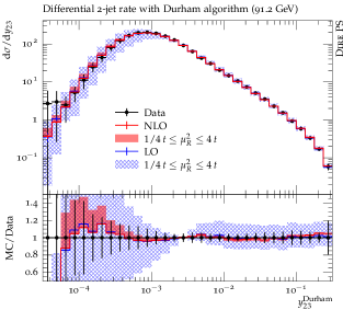
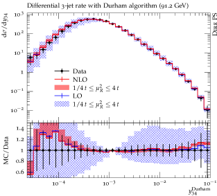
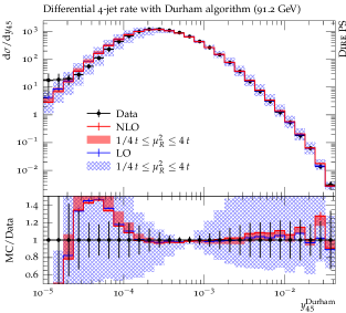
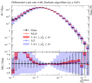
Figure 1 shows predictions from our new implementation compared to leading-order results from the D IRE parton shower for differential jet rates in the Durham scheme compared to experimental results from the JADE and OPAL collaborations Pfeifenschneider et al. (2000). Results have been obtained with D IRE +S HERPA using the default settings of S HERPA version 2.2.3. The perturbative region is to the right of the plots, and $y\sim 2.8\cdot 10^{-3}$ corresponds to the $b$-quark mass. The simulation of nonperturbative effects dominates the predictions below $\sim 10^{-4}$. In the perturbative region, the results are in excellent agreement with the experimental measurements. The shapes of distributions receive only minor changes compared to the leading-order result, however, the uncertainties are greatly reduced.

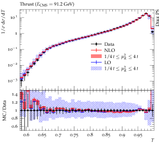
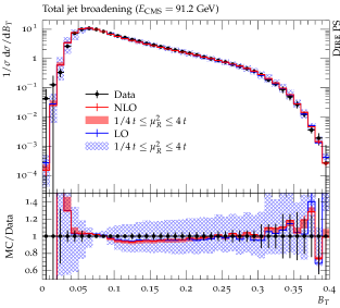
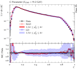
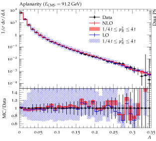
Figure 2 shows a comparison for event shapes measured by the ALEPH collaboration Heister et al. (2004). The perturbative region is to the right of the plot, except for the thrust distribution, where it is to the left. We notice some deviation in the predictions for jet broadening and for the $C$-parameter, which are largely unchanged compared to the leading-order prediction. These deviations are mostly within the 2$\sigma$ uncertainty of the experimental measurements, and they occur close to the nonperturbative region, which indicates that they may be related to hadronization effects.

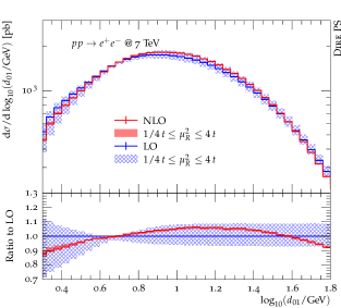
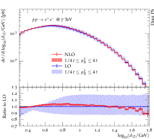
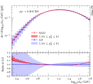
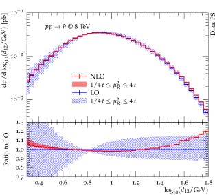
In Figure 3, we illustrate the effect of NLO kernels on differential jet resolutions in Drell-Yan lepton-pair production as well as on Higgs-boson production in gluon fusion. In both cases, the impact of varying the renormalization scale in the parton shower is greatly reduced upon inclusion of NLO corrections, and shape-changes of $\mathcal{O}(10\%)$ can be observed. It is interesting to note that these shape changes have the opposite effect in Drell-Yan lepton pair and Higgs boson production. This effect could not have been obtained by changing the argument of $\alpha_{s}$ at leading order only, as in Eq. (21).

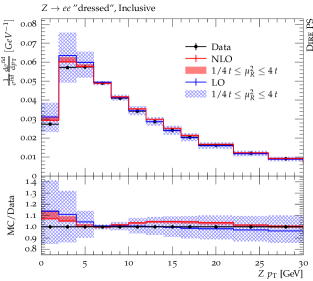
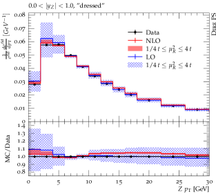
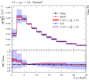
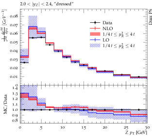
Figure 4 confronts D IRE with Drell-Yan transverse momentum spectra measured by ATLAS Aad et al. (2014). We limit the comparison to the soft and semi-hard region of transverse momenta, $p_{T}<30$ GeV. Parton shower predictions are insufficient in the hard region, and the shower is usually supplemented with fixed-order calculations through matching or merging in order to improve upon this deficiency. Note that no tuning of D IRE +P YTHIA has been performed, neither in the default version nor for the present publication. Our results have been obtained with P YTHIA  8.226, using the NNPDF 3.0 (NLO) PDF set Ball et al. (2015), $\alpha_{s}(M_{Z})=0.118$ throughout the simulation. The ISR/FSR shower cut-off has been set to $3$ GeV², and a primordial transverse momentum of $k_{\perp}=2$ GeV was used. All other parameters are given by the default tune of P YTHIA  8 Skands et al. (2014). NLO corrections improve the agreement with data particularly in the region where resummation has a large impact.

Figure 1: Results for leading and next-to-leading order DGLAP evolution in comparison to LEP data from Pfeifenschneider et al. (2000).

Figure 2: Results for leading and next-to-leading order DGLAP evolution in comparison to LEP data from Heister et al. (2004).

Figure 3: Predictions for leading and next-to-leading order DGLAP evolution for the differential $k_{T}$-jet resolution parameters in $pp\to e^{+}e^{-}+X$ (LHC $\sqrt{s}=7$ TeV) and $pp\to h+X$ (LHC $\sqrt{s}=8$ TeV).

Figure 4: Results for leading and next-to-leading order DGLAP evolution in comparison to ATLAS data from Aad et al. (2014).

V Summary

In this paper we have presented an extension of the parton shower formalism to include, for the first time, the DGLAP evolution at next-to-leading order precision for both initial and final state radiation. The new terms are of order $\alpha_{S}^{2}$, and they fall into three categories: Soft terms $\propto 1/(1-z)$ which are multiplied by the two-loop cusp anomalous dimension, and which are routinely included in parton shower simulations through a suitable rescaling of the argument of the strong coupling. In addition there are genuine, non-trivial higher-order terms which modify already existing leading order terms. Although they are negative over a wide region of phase space we can include them as separate terms through existing reweighting techniques. Finally, there are new structures which correspond to flavor-changing transitions of the type $q\to q^{\prime}$ or $q\to\bar{q}$ and which originate in genuine $1\to 3$ transitions. The algorithm for their simulation is detailed in a separate publication. Including all these terms corresponds to adding the process-independent collinear enhanced NLO corrections present in standard DGLAP evolution into the parton shower. The overall effect of this increased precision is twofold. While for $e^{-}e^{+}$ annihilations to hadrons the central values of distributions experience only marginal shifts, the situation is different for distributions at hadron colliders. This is exemplified by the transverse momentum distribution of $Z$-bosons produced at tree-level in $q\bar{q}$ annihilation and the differential jet rates in $Z$ and Higgs boson production through gluon fusion, respectively, which experience some shifts of up to about 10% relative to corresponding leading order distributions. In both cases, the uncertainty from variations of the renormalization scale by factors of two is significantly reduced when going from leading to next-to-leading order precision. For the first time, we are able to quote a realistic renormalization scale uncertainty as we only add renormalization counterterms which appear at the perturbative order to which we control the expansion of the splitting functions.

While the work presented here represents a significant improvement over existing parton showers, it includes only parts of the higher-order corrections. We did not improve upon the leading color approximation typically used in the parton shower. Ways to include such corrections have been discussed in Plätzer and Sjödahl (2012). Furthermore, we did not include the effect of higher-order soft terms, i.e. the effect of multiple unordered soft emissions. We expect these terms to have only limited impact on inclusive observables such as standard event shapes or the transverse momentum of singlet particles produced at hadron colliders. They will mostly contribute to the further stabilization of perturbative predictions for these observables. However, we appreciate that they will certainly impact on non-global observables such as out-of-cone radiation which in turn renders their inclusion an important task for the future.

Appendix A Next-to-leading order splitting functions

The components of the unregularized space-like quark splitting functions in Eq. (9) are given by

$$\begin{split}p_{qq}^{V(1)}(z)=&\;p^{(0)}_{qq}(z)\left[\Big{(}\beta_{0}\log z+\Gamma^{(2)}\Big{)}-2C_{F}\log z\left(\log(1-z)+\frac{3}{4}\right)+\frac{C_{A}}{2}\log^{2}z\right]-\frac{4}{3}C_{F}T_{F}(1-z)\\ &-C_{F}^{2}\,\left[\left(\frac{3}{2}+\frac{7}{2}z\right)\log z+\frac{1}{2}(1+z)\log^{2}z+5(1-z)\right]+C_{F}C_{A}\,\left[(1+z)\log z+\frac{20}{3}(1-z)\right]\;,\\ \end{split}$$ (22)

$$p_{qq}^{S(1)}(z)=C_{F}T_{F}\bigg{[}-(1+z)\log^{2}z+\left(\frac{8}{3}z^{2}+5z+1\right)\log z-\frac{56}{9}z^{2}+6z-2+\frac{20}{9z}\,\bigg{]}\;.$$ (23)

$$\begin{split}p_{qg}^{(1)}(z)=&\;p_{qg}^{(0)}(z)\bigg{[}\,2\beta_{0}\log(1-z)-T_{F}\left(\frac{4}{3}z+\frac{20}{9}\right)-C_{F}\Big{(}3\log(1-z)+\log^{2}(1-z)\Big{)}\bigg{]}\\ &+C_{F}^{2}\,\bigg{[}-\frac{5}{2}-\frac{7z}{2}+\left(2+\frac{7z}{2}\right)\log z-\left(1-\frac{z}{2}\right)\log^{2}z-2z\log(1-z)\bigg{]}\\ &+C_{F}C_{A}\,\bigg{[}\,\frac{28}{9}+\frac{65z}{18}+\frac{44z^{2}}{9}-\left(12+5z+\frac{8z^{2}}{3}\right)\log z+(4+z)\log^{2}z+2z\log(1-z)\\ &\qquad+S_{2}(z)\hat{p}^{(0)}_{qg}(-z)+\left(\frac{1}{2}-2\log z\log(1-z)+\frac{1}{2}\log^{2}z+\log^{2}(1-z)-\frac{\pi^{2}}{6}\right)\,\hat{p}^{(0)}_{qg}(z)\bigg{]}\;.\end{split}$$ (24)

We use the auxiliary function $S_{2}$ defined in Ellis et al. (1996)

$$\begin{split}S_{2}(z)=\;&-2\,{\rm Li}_{2}\Big{(}\frac{1}{1+z}\Big{)}+\frac{1}{2}\log^{2}z-\log^{2}(1-z)+\frac{\pi^{2}}{6}\;.\end{split}$$ (25)

The unregularized gluon splitting functions at NLO are given by

$$\begin{split}p_{gq}^{(1)}(z)=&\;C_{F}T_{F}\bigg{[}\,p_{gq}^{(0)}(z)\,\bigg{(}2\log^{2}\left(\frac{1-z}{z}\right)-4\log\left(\frac{1-z}{z}\right)-\frac{2\pi^{2}}{3}+10\bigg{)}\\ &\quad\quad+4-9z-(1-4z)\log z-(1-2z)\log^{2}z+4\log(1-z)\bigg{]}+C_{A}S_{2}(z)p_{gq}^{(0)}(-z)\\ &+C_{A}T_{F}\bigg{[}\,p_{gq}^{(0)}(z)\bigg{(}\,-\log^{2}z+\frac{44}{3}\log z-2\log^{2}(1-z)+4\log(1-z)+\frac{\pi^{2}}{3}-\frac{218}{9}\bigg{)}\\ &\quad\quad+\frac{182}{9}+\frac{14z}{9}+\frac{40}{9z}+\left(\frac{136z}{3}-\frac{38}{3}\right)\log z-4\log(1-z)-(2+8z)\log^{2}z\bigg{]}\;.\end{split}$$ (26)

$$\begin{split}p_{gg}^{(1)}(z)=&\;p^{(0)}_{gg}(z)\,\bigg{[}\,\Gamma^{(2)}+C_{A}\bigg{(}-2\log z\log(1-z)+\frac{1}{2}\log^{2}z\bigg{)}\bigg{]}\,+\,C_{A}S_{2}(z)p^{(0)}_{gg}(-z)\\ &+C_{F}T_{F}\,\bigg{[}\,-16+8z+\frac{20z^{2}}{3}+\frac{4}{3z}-(6+10z)\log z-(2+2z)\log^{2}z\bigg{]}\\ &+C_{A}T_{F}\bigg{[}\,2-2z+\frac{26}{9}\left(z^{2}-\frac{1}{z}\right)-\frac{4}{3}(1+z)\log z\bigg{]}\\ &+C_{A}^{2}\bigg{[}\,\frac{27}{2}(1-z)+\frac{67}{9}\left(z^{2}-\frac{1}{z}\right)-\left(\frac{25}{3}-\frac{11z}{3}+\frac{44z^{2}}{3}\right)\log z+4(1+z)\log^{2}z\bigg{]}\,.\end{split}$$ (27)

The components of the unregularized time-like quark splitting functions in Eq. (9) are given by

$$\begin{split}p_{qq}^{V(1)}(z)=&\;p^{(0)}_{qq}(z)\left[\Big{(}\beta_{0}\log z+\Gamma^{(2)}\Big{)}+2C_{F}\log z\left(\log\frac{1-z}{z}+\frac{3}{4}\right)+\frac{C_{A}}{2}\log^{2}z\right]-\frac{4}{3}C_{F}T_{F}(1-z)\\ &-C_{F}^{2}\,\left[\left(\frac{7}{2}+\frac{3}{2}z\right)\log z-\frac{1}{2}(1+z)\log^{2}z+5(1-z)\right]+C_{F}C_{A}\,\left[(1+z)\log z+\frac{20}{3}(1-z)\right]\;,\\ \end{split}$$ (28)

$$p_{qq}^{S(1)}(z)=\;C_{F}T_{F}\left[\,(1+x)\log^{2}x-\left(\frac{8}{3}z^{2}+9z+5\right)\log z+\frac{56}{9}z^{2}+4z-8-\frac{20}{9z}\,\right]\;.$$ (29)

$$\begin{split}p_{qg}^{(1)}(z)=&\;C_{F}^{2}\,\bigg{[}\,\hat{p}_{qg}^{(0)}(z)\bigg{(}\,\log^{2}(1-z)+4\log z\log(1-z)-8S_{1}(z)-\frac{4}{3}\pi^{2}\bigg{)}\\ &\quad\quad-\frac{1}{2}+\frac{9z}{2}-\left(8-\frac{z}{2}\right)\log z+2z\log(1-z)+\left(1-\frac{z}{2}\right)\log^{2}z\bigg{]}+C_{A}S_{2}(z)p_{qg}^{(0)}(-z)\\ &+C_{F}C_{A}\,\bigg{[}\,\frac{62}{9}-\frac{35z}{18}-\frac{44z^{2}}{9}+\left(2+12z+\frac{8}{3}z^{2}\right)\log z-2z\log(1-z)-(4+z)\log^{2}z\\ &\qquad-\hat{p}_{qg}^{(0)}(z)\bigg{(}2\log z\log(1-z)+3\log z+\frac{3}{2}\log^{2}z+\log^{2}(1-z)-8S_{1}(z)-\frac{7\pi^{2}}{6}-\frac{17}{18}\bigg{)}\bigg{]}\;.\end{split}$$ (30)

We use the auxiliary function $S_{1}$ defined in Ellis et al. (1996)

$$\begin{split}S_{1}(z)=\;&{\rm Li}_{2}(z)+\log z\log(1-z)-\frac{\pi^{2}}{6}\;.\end{split}$$ (31)

The unregularized gluon splitting functions at NLO are given by

$$\begin{split}p_{gq}^{(1)}(z)=&\;T^{2}_{F}\bigg{[}\,-\frac{8}{3}-p_{gq}^{(0)}(z)\left(\frac{16}{9}+\frac{8}{3}\log z+\frac{8}{3}\log(1-z)\right)\bigg{]}\\ &+C_{F}T_{F}\bigg{[}\,p_{gq}^{(0)}(z)\,\left(-2\log^{2}(z(1-z))-2\log\left(\frac{1-z}{z}\right)+16S_{1}(z)+2\pi^{2}-10\right)\\ &\qquad-2+3z-(7-8z)\log z-4\log(1-z)+(1-2z)\log^{2}z\bigg{]}+C_{A}S_{2}(z)p_{gq}^{(0)}(-z)\\ &+C_{A}T_{F}\bigg{[}\,-\frac{152}{9}+\frac{166z}{9}-\frac{40}{9z}-\left(\frac{76z}{3}+\frac{4}{3}\right)\log z+4\log(1-z)+(2+8z)\log^{2}z\\ &\qquad+\hat{p}_{gq}^{(0)}(z)\bigg{(}\,8\log z\log(1-z)-\log^{2}z-\frac{4}{3}\log z+\frac{10}{3}\log(1-z)\\ &\qquad\qquad+2\log^{2}(1-z)-16S_{1}(z)-\frac{7\pi^{2}}{3}+\frac{178}{9}\bigg{)}\bigg{]}\\ \end{split}$$ (32)

$$\begin{split}p_{gg}^{(1)}(z)=&\;p^{(0)}_{gg}(z)\,\bigg{[}2\beta_{0}\log z+\Gamma^{(2)}+\,C_{A}\log z\,\bigg{(}2\log(1-z)-\frac{3}{2}\log^{2}z\bigg{)}\bigg{]}\,+\,C_{A}S_{2}(z)p^{(0)}_{gg}(-z)\\ &+C_{F}T_{F}\,\bigg{[}\,-4+12z-\frac{164}{9}z^{2}\left(10+14z+\frac{16z^{2}}{3}+\frac{16}{3z}\right)\log z+\frac{92}{9z}+2(1+z)\log^{2}z\bigg{]}\\ &+C_{A}T_{F}\bigg{[}\,2-2z+\frac{26}{9}\left(z^{2}-\frac{1}{z}\right)-\frac{4}{3}(1+z)\log z\bigg{]}\\ &+C_{A}^{2}\bigg{[}\,\frac{27}{2}(1-z)+\frac{67}{9}\left(z^{2}-\frac{1}{z}\right)+\left(\frac{11}{3}-\frac{25}{3}z+\frac{44}{3z}\right)\log z-4(1+z)\log^{2}z\bigg{]}\,.\end{split}$$ (33)

References

- Buckley et al. (2011) A. Buckley et al., Phys. Rept. 504, 145 (2011), arXiv:1101.2599 [hep-ph] .
- Fox and Wolfram (1980) G. C. Fox and S. Wolfram, Nucl. Phys. B168, 285 (1980).
- Sjöstrand (1985) T. Sjöstrand, Phys. Lett. B157, 321 (1985).
- Azimov et al. (1985a) Y. I. Azimov, Y. L. Dokshitzer, V. A. Khoze, and S. I. Troyan, Z. Phys. C27, 65 (1985a).
- Azimov et al. (1985b) Y. I. Azimov, Y. L. Dokshitzer, V. A. Khoze, and S. I. Troian, Phys. Lett. 165B, 147 (1985b).
- Webber (1984) B. R. Webber, Nucl. Phys. B238, 492 (1984).
- Marchesini and Webber (1984) G. Marchesini and B. R. Webber, Nucl. Phys. B238, 1 (1984).
- Marchesini and Webber (1988) G. Marchesini and B. R. Webber, Nucl. Phys. B310, 461 (1988).
- Gustafson and Pettersson (1988) G. Gustafson and U. Pettersson, Nucl. Phys. B306, 746 (1988).
- Lönnblad (1992) L. Lönnblad, Comput. Phys. Commun. 71, 15 (1992).
- Bengtsson and Sjöstrand (1987a) M. Bengtsson and T. Sjöstrand, Nucl. Phys. B289, 810 (1987a).
- Bengtsson and Sjöstrand (1987b) M. Bengtsson and T. Sjöstrand, Phys. Lett. B185, 435 (1987b).
- Frixione and Webber (2002) S. Frixione and B. R. Webber, JHEP 06, 029 (2002), hep-ph/0204244 .
- Höche et al. (2012) S. Höche, F. Krauss, M. Schönherr, and F. Siegert, JHEP 09, 049 (2012), arXiv:1111.1220 [hep-ph] .
- Hamilton et al. (2013a) K. Hamilton, P. Nason, C. Oleari, and G. Zanderighi, JHEP 05, 082 (2013a), arXiv:1212.4504 [hep-ph] .
- Hamilton et al. (2013b) K. Hamilton, P. Nason, E. Re, and G. Zanderighi, JHEP 1310, 222 (2013b), arXiv:1309.0017 [hep-ph] .
- Höche et al. (2015) S. Höche, Y. Li, and S. Prestel, Phys. Rev. D91, 074015 (2015), arXiv:1405.3607 [hep-ph] .
- Höche et al. (2014) S. Höche, Y. Li, and S. Prestel, Phys. Rev. D90, 054011 (2014), arXiv:1407.3773 [hep-ph] .
- Catani et al. (2001) S. Catani, F. Krauss, R. Kuhn, and B. R. Webber, JHEP 11, 063 (2001), hep-ph/0109231 .
- Lönnblad (2002) L. Lönnblad, JHEP 05, 046 (2002), hep-ph/0112284 .
- Krauss (2002) F. Krauss, JHEP 0208, 015 (2002), hep-ph/0205283 .
- Mangano et al. (2007) M. L. Mangano, M. Moretti, F. Piccinini, and M. Treccani, JHEP 01, 013 (2007), hep-ph/0611129 .
- Alwall et al. (2008) J. Alwall et al., Eur. Phys. J. C53, 473 (2008), arXiv:0706.2569 [hep-ph] .
- Höche et al. (2009) S. Höche, F. Krauss, S. Schumann, and F. Siegert, JHEP 05, 053 (2009), arXiv:0903.1219 [hep-ph] .
- Hamilton and Nason (2010) K. Hamilton and P. Nason, JHEP 06, 039 (2010), arXiv:1004.1764 [hep-ph] .
- Höche et al. (2013) S. Höche, F. Krauss, M. Schönherr, and F. Siegert, JHEP 1304, 027 (2013), arXiv:1207.5030 [hep-ph] .
- Plätzer (2013) S. Plätzer, JHEP 1308, 114 (2013), arXiv:1211.5467 [hep-ph] .
- Lönnblad and Prestel (2013a) L. Lönnblad and S. Prestel, JHEP 1303, 166 (2013a), arXiv:1211.7278 [hep-ph] .
- Lönnblad and Prestel (2013b) L. Lönnblad and S. Prestel, JHEP 1302, 094 (2013b), arXiv:1211.4827 [hep-ph] .
- Frederix and Frixione (2012) R. Frederix and S. Frixione, JHEP 1212, 061 (2012), arXiv:1209.6215 [hep-ph] .
- Sjöstrand and Skands (2005) T. Sjöstrand and P. Z. Skands, Eur. Phys. J. C39, 129 (2005), hep-ph/0408302 .
- Schumann and Krauss (2008) S. Schumann and F. Krauss, JHEP 03, 038 (2008), arXiv:0709.1027 [hep-ph] .
- Dinsdale et al. (2007) M. Dinsdale, M. Ternick, and S. Weinzierl, Phys. Rev. D76, 094003 (2007), arXiv:0709.1026 [hep-ph] .
- Winter and Krauss (2008) J.-C. Winter and F. Krauss, JHEP 07, 040 (2008), arXiv:0712.3913 [hep-ph] .
- Giele et al. (2008) W. T. Giele, D. A. Kosower, and P. Z. Skands, Phys. Rev. D78, 014026 (2008), arXiv:0707.3652 [hep-ph] .
- Plätzer and Gieseke (2011) S. Plätzer and S. Gieseke, JHEP 01, 024 (2011), arXiv:0909.5593 [hep-ph] .
- Ritzmann et al. (2013) M. Ritzmann, D. A. Kosower, and P. Skands, Phys. Lett. B718, 1345 (2013), arXiv:1210.6345 [hep-ph] .
- Höche and Prestel (2015) S. Höche and S. Prestel, Eur. Phys. J. C75, 461 (2015), arXiv:1506.05057 [hep-ph] .
- Gieseke et al. (2003) S. Gieseke, P. Stephens, and B. Webber, JHEP 12, 045 (2003), arXiv:hep-ph/0310083 .
- Kato and Munehisa (1987) K. Kato and T. Munehisa, Phys. Rev. D36, 61 (1987).
- Kato and Munehisa (1989) K. Kato and T. Munehisa, Phys. Rev. D39, 156 (1989).
- Kato and Munehisa (1991) K. Kato and T. Munehisa, Comput. Phys. Commun. 64, 67 (1991).
- Kato et al. (1992) K. Kato, T. Munehisa, and H. Tanaka, Z. Phys. C54, 397 (1992).
- Hartgring et al. (2013) L. Hartgring, E. Laenen, and P. Skands, JHEP 10, 127 (2013), arXiv:1303.4974 [hep-ph] .
- Li and Skands (2016) H. T. Li and P. Skands, (2016), arXiv:1611.00013 [hep-ph] .
- Jadach et al. (2011) S. Jadach, A. Kusina, M. Skrzypek, and M. Slawinska, JHEP 08, 012 (2011), arXiv:1102.5083 [hep-ph] .
- Gituliar et al. (2014) O. Gituliar, S. Jadach, A. Kusina, and M. Skrzypek, Phys. Lett. B732, 218 (2014), arXiv:1401.5087 [hep-ph] .
- Jadach et al. (2016) S. Jadach, A. Kusina, W. Placzek, and M. Skrzypek, JHEP 08, 092 (2016), arXiv:1606.01238 [hep-ph] .
- Curci et al. (1980) G. Curci, W. Furmanski, and R. Petronzio, Nucl. Phys. B175, 27 (1980).
- Furmanski and Petronzio (1980) W. Furmanski and R. Petronzio, Phys. Lett. B97, 437 (1980).
- Floratos et al. (1981a) E. G. Floratos, R. Lacaze, and C. Kounnas, Phys. Lett. B98, 89 (1981a).
- Floratos et al. (1981b) E. G. Floratos, R. Lacaze, and C. Kounnas, Phys. Lett. B98, 285 (1981b).
- Heinrich and Kunszt (1998) G. Heinrich and Z. Kunszt, Nucl. Phys. B519, 405 (1998), hep-ph/9708334 .
- (54) R. K. Ellis and W. Vogelsang, hep-ph/9602356 .
- Höche and Prestel (2017) S. Höche and S. Prestel, (2017), arXiv:1705.00742 [hep-ph] .
- Catani et al. (1991) S. Catani, B. R. Webber, and G. Marchesini, Nucl. Phys. B349, 635 (1991).
- Höche et al. (2010) S. Höche, S. Schumann, and F. Siegert, Phys. Rev. D81, 034026 (2010), arXiv:0912.3501 [hep-ph] .
- Lönnblad (2012) L. Lönnblad, (2012), arXiv:1211.7204 [hep-ph] .
- Gribov and Lipatov (1972) V. N. Gribov and L. N. Lipatov, Sov. J. Nucl. Phys. 15, 438 (1972).
- Dokshitzer (1977) Y. L. Dokshitzer, Sov. Phys. JETP 46, 641 (1977).
- Altarelli and Parisi (1977) G. Altarelli and G. Parisi, Nucl. Phys. B126, 298 (1977).
- Jadach and Skrzypek (2004) S. Jadach and M. Skrzypek, Acta Phys. Polon. B35, 745 (2004), hep-ph/0312355 .
- Procura and Stewart (2010) M. Procura and I. W. Stewart, Phys. Rev. D81, 074009 (2010), [Erratum: Phys. Rev.D83,039902(2011)], arXiv:0911.4980 [hep-ph] .
- Jain et al. (2011) A. Jain, M. Procura, and W. J. Waalewijn, JHEP 05, 035 (2011), arXiv:1101.4953 [hep-ph] .
- Becher and Neubert (2011) T. Becher and M. Neubert, Eur. Phys. J. C71, 1665 (2011), arXiv:1007.4005 [hep-ph] .
- (66) J. R. Andersen et al., arXiv:1605.04692 [hep-ph] .
- Sjöstrand et al. (2015) T. Sjöstrand, S. Ask, J. R. Christiansen, R. Corke, N. Desai, P. Ilten, S. Mrenna, S. Prestel, C. O. Rasmussen, and P. Z. Skands, Comput. Phys. Commun. 191, 159 (2015), arXiv:1410.3012 [hep-ph] .
- Gleisberg et al. (2004) T. Gleisberg, S. Höche, F. Krauss, A. Schälicke, S. Schumann, and J. Winter, JHEP 02, 056 (2004), hep-ph/0311263 .
- Gleisberg et al. (2009) T. Gleisberg, S. Höche, F. Krauss, M. Schönherr, S. Schumann, F. Siegert, and J. Winter, JHEP 02, 007 (2009), arXiv:0811.4622 [hep-ph] .
- Pfeifenschneider et al. (2000) P. Pfeifenschneider et al. (JADE and OPAL), Eur. Phys. J. C17, 19 (2000), arXiv:hep-ex/0001055 .
- Heister et al. (2004) A. Heister et al. (ALEPH), Eur. Phys. J. C35, 457 (2004).
- Aad et al. (2014) G. Aad et al. (ATLAS), JHEP 09, 145 (2014), arXiv:1406.3660 [hep-ex] .
- Ball et al. (2015) R. D. Ball et al. (NNPDF), JHEP 04, 040 (2015), arXiv:1410.8849 [hep-ph] .
- Skands et al. (2014) P. Skands, S. Carrazza, and J. Rojo, Eur. Phys. J. C74, 3024 (2014), arXiv:1404.5630 [hep-ph] .
- Plätzer and Sjödahl (2012) S. Plätzer and M. Sjödahl, JHEP 1207, 042 (2012), arXiv:1201.0260 [hep-ph] .
- Ellis et al. (1996) R. K. Ellis, W. J. Stirling, and B. R. Webber, QCD and collider physics, 1st ed., Vol. 8 (Cambridge Monogr. Part. Phys. Nucl. Phys. Cosmol., 1996) p. 435.