Quaternion Gaussian matrices satisfy the RIP

Agnieszka Badeńska1 Łukasz Błaszczyk1,2
badenska@mini.pw.edu.pl l.blaszczyk@mini.pw.edu.pl
1 Faculty of Mathematics 2 Institute of Radioelectronics
and Information Science and Multimedia Technology
Warsaw University of Technology Warsaw University of Technology
ul. Koszykowa 75 ul. Nowowiejska 15/19
00-662 Warszawa, Poland 00-665 Warszawa, Poland

Keywords: quaternion Gaussian random matrix, restricted isometry property, sparse signals.


Abstract

We prove that quaternion Gaussian random matrices satisfy the restricted isometry property (RIP) with overwhelming probability. We also explain why the restricted isometry random variables (RIV) approach is not appropriate for drawing conclusions on restricted isometry constants.

1 Introduction

One of the conditions which guarantees exact reconstruction of a sparse signal (real, complex or quaternion) – by 1subscript1\ell_{1}-norm minimization – from a few number of its linear measurements is that the measurement matrix satisfies the celebrated restricted isometry property (RIP) with a sufficiently small constant. The notion of restricted isometry constants was introduced by Candès and Tao in [4] and repeatedly considered afterwards. The concept was also generalized to quaternion signals [1, 2].

Definition 1.1.

Let 𝚽m×n𝚽superscript𝑚𝑛\mathbf{\Phi}\in\mathbb{H}^{m\times n} and s{1,,n}𝑠1𝑛s\in\{1,\ldots,n\}. The s𝑠s-restricted isometry constant of 𝚽𝚽\mathbf{\Phi} is the smallest number δssubscript𝛿𝑠\delta_{s} with the property that

(1δs)𝕩22𝚽𝕩22(1+δs)𝕩221subscript𝛿𝑠superscriptsubscriptdelimited-∥∥𝕩22superscriptsubscriptdelimited-∥∥𝚽𝕩221subscript𝛿𝑠superscriptsubscriptdelimited-∥∥𝕩22\left(1-\delta_{s}\right)\left\lVert{\mathbbm{x}}\right\rVert_{2}^{2}\leq\left\lVert{\mathbf{\Phi}\mathbbm{x}}\right\rVert_{2}^{2}\leq\left(1+\delta_{s}\right)\left\lVert{\mathbbm{x}}\right\rVert_{2}^{2} (1.1)

for all s𝑠s-sparse quaternion vectors 𝕩n𝕩superscript𝑛\mathbbm{x}\in\mathbb{H}^{n}.

Recall that we call a vector (signal) s𝑠s-sparse if it has at most s𝑠s nonzero coordinates and \mathbb{H} denotes the quaternion algebra.

It is known that e.g. real Gaussian and Bernoulli random matrices, also partial Discrete Fourier Transform matrices satisfy the RIP (with overwhelming probability) [5], however, until recently there were no known examples of quaternion matrices satisfying this condition. In [1, Lemma 3.2] we proved that if a real matrix 𝚽m×n𝚽superscript𝑚𝑛\mathbf{\Phi}\in\mathbb{R}^{m\times n} satisfies the inequalities (1.1) for real s𝑠s-sparse vectors 𝕩n𝕩superscript𝑛\mathbbm{x}\in\mathbb{R}^{n}, then it also satisfies it – with the same constant δssubscript𝛿𝑠\delta_{s} – for s𝑠s-sparse quaternion vectors 𝕩n𝕩superscript𝑛\mathbbm{x}\in\mathbb{H}^{n}. This was a first step towards developing theoretical background of compressed sensing methods in the quaternion algebra, since we also showed that it is possible to reconstruct sparse quaternion vectors from a small number of their linear measurements if an appropriate restricted isometry constant of a real measurement matrix 𝚽m×n𝚽superscript𝑚𝑛\mathbf{\Phi}\in\mathbb{R}^{m\times n} is sufficiently small [1, Corollary 5.1].

Later we extended the above-mentioned result to the full quaternion setting – with the expected assumption that a quaternion measurement matrix 𝚽m×n𝚽superscript𝑚𝑛\mathbf{\Phi}\in\mathbb{H}^{m\times n} satisfies the RIP with a sufficiently small constant [2, Corollary 5.1]. The question of existence of quaternion matrices satisfying the RIP was, however, still open. Let us also mention a very interesting recent result of N. Gomes, S. Hartmann and U. Kähler concerning the quaternion Fourier matrices – arising in color representation of images [6]. They showed that with high probability such matrices allow a sparse reconstruction (again by 1subscript1\ell_{1}-norm minimization) [6, Theorem 3.2]. Their proof is straightforward and does not use the RIP notion, however, they also point out that it is not clear whether quaternion sampling matrices fulfill the RIP condition.

It has been believed that quaternion Gaussian random matrices satisfy the RIP and, therefore, they have been widely used in numerical experiments [3, 7, 17] but there was a lack of theoretical justification for this conviction. In this article we prove that this hypothesis is true, i.e. quaternion Gaussian random matrices satisfy the RIP, and we provide estimates on matrix sizes that guarantee the RIP with overwhelming probability (Theorem 4.2). The existence of quaternion matrices satisfying the RIP, together with the main results of [2], constitute the theoretical foundation of the classical compressed sensing methods in the quaternion algebra.

Apart from the aforementioned numerical experiments, our main motivation was the article [2], which revealed the need for quaternion matrices satisfying the RIP. In our research we got interested in the articles [8, 9, 10], the authors of which claim they had found a simpler proof of the RIP for real and complex Gaussian random matrices. This brought us to study the ratio random variable, so-called Rayleigh quotient

=𝚽𝕩22𝕩22superscriptsubscriptdelimited-∥∥𝚽𝕩22superscriptsubscriptdelimited-∥∥𝕩22\mathcal{R}=\frac{\left\lVert{\mathbf{\Phi}\mathbbm{x}}\right\rVert_{2}^{2}}{\left\lVert{\mathbbm{x}}\right\rVert_{2}^{2}}

for 𝚽m×n𝚽superscript𝑚𝑛\mathbf{\Phi}\in\mathbb{H}^{m\times n} and non-zero, s𝑠s-sparse vector 𝕩n𝕩superscript𝑛\mathbbm{x}\in\mathbb{H}^{n}, and eventually finding its distribution, i.e. Γ(2m,2m)Γ2𝑚2𝑚\Gamma(2m,2m), which does not depend on 𝕩𝕩\mathbbm{x}, (Lemma 3.1). Its mean (expectation) equals 111 and its variance equals 12m12𝑚\frac{1}{2m}. Recall that in the real case \mathcal{R} has distribution Γ(m2,m2)Γ𝑚2𝑚2\Gamma\left(\frac{m}{2},\frac{m}{2}\right) with the same mean but four times bigger variance 2m2𝑚\frac{2}{m} [8]. It clearly explains higher rate of correct sparse signals reconstructions in the quaternion case in compare with the real case of the same size (see [2, Section 6]).

Having proved Lemma 3.1, we were initially hoping to mimic the approach from [8, 9, 10] to obtain the proof of the RIP for quaternion Gaussian matrices, however, in our humble opinion it contains certain inaccuracies, which we want to briefly point out before proceeding further (we refer to [8] for more details). The authors call a vector 𝕩𝕩\mathbbm{x} s𝑠s-sparse if it has exactly s𝑠s non-zero coordinates and introduce left and right s𝑠s-restricted isometry constants (RIC) as

δsL=1min#supp𝕩=s𝚽𝕩22𝕩22,δsR=max#supp𝕩=s𝚽𝕩22𝕩221,formulae-sequencesuperscriptsubscript𝛿𝑠𝐿1subscript#supp𝕩𝑠superscriptsubscriptdelimited-∥∥𝚽𝕩22superscriptsubscriptdelimited-∥∥𝕩22superscriptsubscript𝛿𝑠𝑅subscript#supp𝕩𝑠superscriptsubscriptdelimited-∥∥𝚽𝕩22superscriptsubscriptdelimited-∥∥𝕩221\delta_{s}^{L}=1-\min_{\#\operatorname{supp}\,\mathbbm{x}=s}\frac{\left\lVert{\mathbf{\Phi}\mathbbm{x}}\right\rVert_{2}^{2}}{\left\lVert{\mathbbm{x}}\right\rVert_{2}^{2}},\qquad\delta_{s}^{R}=\max_{\#\operatorname{supp}\,\mathbbm{x}=s}\frac{\left\lVert{\mathbf{\Phi}\mathbbm{x}}\right\rVert_{2}^{2}}{\left\lVert{\mathbbm{x}}\right\rVert_{2}^{2}}-1, (1.2)

where #supp𝕩#supp𝕩\#\operatorname{supp}\,\mathbbm{x} denotes the cardinality of the support set of 𝕩𝕩\mathbbm{x} (i.e. the number of its nonzero coordinates). Note that it differs substantially from our approach from Definition 1.1 (max(δsL,δsR)superscriptsubscript𝛿𝑠𝐿superscriptsubscript𝛿𝑠𝑅\max(\delta_{s}^{L},\delta_{s}^{R}) might be smaller than δssubscript𝛿𝑠\delta_{s} and we loose monotonicity of δssubscript𝛿𝑠\delta_{s} with respect to s𝑠s). Moreover, the set of vectors with a fixed cardinality of the support does not have the structure of a module over the ring \mathbb{H} anymore, hence the above variables may not be well-defined (one might need to use inf/supinfimumsupremum\inf/\sup instead).

After noticing that all ratio random variables 𝚽𝕩22𝕩22superscriptsubscriptdelimited-∥∥𝚽𝕩22superscriptsubscriptdelimited-∥∥𝕩22\frac{\left\lVert{\mathbf{\Phi}\mathbbm{x}}\right\rVert_{2}^{2}}{\left\lVert{\mathbbm{x}}\right\rVert_{2}^{2}} have the same distribution, which does not depend on the choice of 𝕩𝕩\mathbbm{x}, the aforementioned authors only consider one vector 𝕩Ssuperscript𝕩𝑆\mathbbm{x}^{S} with supp𝕩S=Ssuppsuperscript𝕩𝑆𝑆\operatorname{supp}\,\mathbbm{x}^{S}=S for every support set S𝑆S with #S=s#𝑆𝑠\#S=s and define the following variable, called restricted isometry random variable (RIV)

ΔsR=maxS:#S=s{𝚽𝕩S22𝕩S22 for some 𝕩S with supp𝕩S=S}1superscriptsubscriptΔ𝑠𝑅subscript:𝑆#𝑆𝑠superscriptsubscriptdelimited-∥∥𝚽superscript𝕩𝑆22superscriptsubscriptdelimited-∥∥superscript𝕩𝑆22 for some superscript𝕩𝑆 with suppsuperscript𝕩𝑆𝑆1\Delta_{s}^{R}=\max_{S:\#S=s}\left\{\frac{\left\lVert{\mathbf{\Phi}\mathbbm{x}^{S}}\right\rVert_{2}^{2}}{\left\lVert{\mathbbm{x}^{S}}\right\rVert_{2}^{2}}\;\text{ for some }\mathbbm{x}^{S}\text{ with }\operatorname{supp}\,\mathbbm{x}^{S}=S\right\}-1

(ΔsLsuperscriptsubscriptΔ𝑠𝐿\Delta_{s}^{L} analogously), that is omitting max/min\max/\min over uncountable sets of vectors supported on appropriate sets S𝑆S. That is true that for a fixed vector and full ensemble of Gaussian matrices all Rayleigh quotients \mathcal{R} have the same distribution, yet the vector that realizes the max/min\max/\min on a fixed support set S𝑆S depends on the realization matrix in general, therefore the distribution of max{𝚽𝕩22𝕩22:supp𝕩=S}:superscriptsubscriptdelimited-∥∥𝚽𝕩22superscriptsubscriptdelimited-∥∥𝕩22supp𝕩𝑆\max\left\{\frac{\left\lVert{\mathbf{\Phi}\mathbbm{x}}\right\rVert_{2}^{2}}{\left\lVert{\mathbbm{x}}\right\rVert_{2}^{2}}:\operatorname{supp}\mathbbm{x}=S\right\} very likely differs from the distribution of a single \mathcal{R} for a fixed vector. Therefore, one cannot draw any conclusions concerning δsLsuperscriptsubscript𝛿𝑠𝐿\delta_{s}^{L}, δsRsuperscriptsubscript𝛿𝑠𝑅\delta_{s}^{R} or δssubscript𝛿𝑠\delta_{s} based on the upper estimates of ΔsLsuperscriptsubscriptΔ𝑠𝐿\Delta_{s}^{L}, ΔsRsuperscriptsubscriptΔ𝑠𝑅\Delta_{s}^{R} since obviously

ΔsLδsLδsandΔsRδsRδs.formulae-sequencesuperscriptsubscriptΔ𝑠𝐿superscriptsubscript𝛿𝑠𝐿subscript𝛿𝑠andsuperscriptsubscriptΔ𝑠𝑅superscriptsubscript𝛿𝑠𝑅subscript𝛿𝑠\Delta_{s}^{L}\leq\delta_{s}^{L}\leq\delta_{s}\quad\text{and}\quad\Delta_{s}^{R}\leq\delta_{s}^{R}\leq\delta_{s}.

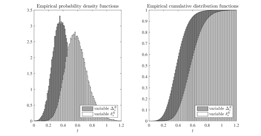
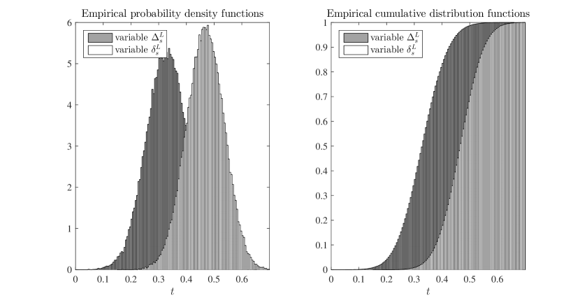
Empirical distributions of RICs and RIVs are presented in section 5 in Fig. 1 and 2.

Finally, the authors of [8] claim to have derived the precise distribution functions of ΔsRsuperscriptsubscriptΔ𝑠𝑅\Delta_{s}^{R} and ΔsLsuperscriptsubscriptΔ𝑠𝐿\Delta_{s}^{L} using, what they call, an ’i.i.d. representation’, even though they admit that the Rayleigh quotients for different supports are not independent if the support sets intersect. In fact, they suggest a lower estimate of the cumulative distribution functions (CDF) of the RIVs by the CDF of a maximum of (ns)binomial𝑛𝑠{n\choose s} (the number of support sets) i.i.d. variables of the same distribution as \mathcal{R} [8, Appendix E, Step 1], however, their proof is very unsatisfactory due to the lack of theoretical justification for the presented inequalities. For the case of two random variables what they really use is so-called positive dependence, proved for certain distributions (including Gamma and Chi-square) in more general case, i.e.

(X1A,X2A)(X1A)(X2A)formulae-sequencesubscript𝑋1𝐴subscript𝑋2𝐴subscript𝑋1𝐴subscript𝑋2𝐴\mathbb{P}(X_{1}\in A,X_{2}\in A)\geq\mathbb{P}(X_{1}\in A)\cdot\mathbb{P}(X_{2}\in A)

for all measurable sets A𝐴A\subset\mathbb{R} (see e.g. [11]). For the bigger number of variables with Gamma distribution this result was extended to a certain extent [13] but – to our best knowledge – there is no proof for the general case.

To sum up, it might be somewhat interesting to study the RIVs in the compressed sensing analysis, however, it brings no information on the upper estimate of the restricted isometry constants. Therefore, this approach is not useful for attempts of proving the RIP. In fact, the eigenvalue approach, i.e. analysis of moduli of eigenvalues of Hermitian matrices 𝚽S𝚽Ssuperscriptsubscript𝚽𝑆subscript𝚽𝑆\mathbf{\Phi}_{S}^{*}\mathbf{\Phi}_{S}, criticized by the authors of [8], is the right direction – it is well known that the restricted isometry constants can be expressed in terms of these eigenvalues (also in the quaternion case – cf. [2, Lemma 2.1]). Currently however, we do not know distribution of the eigenvalues of 𝚽S𝚽Ssuperscriptsubscript𝚽𝑆subscript𝚽𝑆\mathbf{\Phi}_{S}^{*}\mathbf{\Phi}_{S} in the quaternion case.

That is why our proof of the RIP of quaternion Gaussian random matrices refers to the classical approach for real sub-Gaussian random matrices [5, section 9.1], which uses the notion of sub-exponential (locally sub-Gaussian) random variables and a γ𝛾\gamma-covering of a unit ball. We are aware that our result (Theorem 4.2) is not optimal, and in the current form only applies to the case of big n𝑛n and very small s𝑠s, but it is a first step towards further thorough analysis of the quaternion random matrices and their applications in compressed sensing.

The article is organized as follows. First, we briefly recall basic facts about the quaternion algebra and quaternion matrices. Third section is devoted to quaternion random variables and matrices. We define the quaternion Gaussian random variable with mean zero and variance σ2superscript𝜎2\sigma^{2}, denoted by X𝒩(0,σ2)similar-to𝑋subscript𝒩0superscript𝜎2X\sim\mathcal{N}_{\mathbb{H}}\left(0,\sigma^{2}\right), where in particular we always assume independence of its components – note that this aspect was not clear in [17]. We also provide distribution of the Rayleigh quotient \mathcal{R} for quaternion Gaussian random matrices and justify that it is sub-exponential with appropriate parameters. In the fourth section we prove the main result of the article, i.e. the RIP for quaternion Gaussian random matrices. Finally, we present outcomes of numerical simulations illustrating the theoretical considerations and we conclude with a short résumé of the obtained results and our further research perspectives.

2 Quaternions

Denote by \mathbb{H} the algebra of (Hamilton or real) quaternions

q=a+b𝐢+c𝐣+d𝐤,wherea,b,c,dformulae-sequence𝑞𝑎𝑏𝐢𝑐𝐣𝑑𝐤where𝑎𝑏𝑐𝑑q=a+b\mathbf{i}+c\mathbf{j}+d\mathbf{k},\quad\textrm{where}\quad a,b,c,d\in\mathbb{R}

endowed with the standard norm

|q|=qq¯=a2+b2+c2+d2,𝑞𝑞¯𝑞superscript𝑎2superscript𝑏2superscript𝑐2superscript𝑑2|q|=\sqrt{q\overline{q}}=\sqrt{a^{2}+b^{2}+c^{2}+d^{2}},

where q¯=ab𝐢c𝐣d𝐤¯𝑞𝑎𝑏𝐢𝑐𝐣𝑑𝐤\overline{q}=a-b\mathbf{i}-c\mathbf{j}-d\mathbf{k} is the conjugate of q𝑞q. Recall that multiplication is associative but in general not commutative in the quaternion algebra and is defined by the following rules

𝐢2=𝐣2=𝐤2=𝐢𝐣𝐤=1and𝐢𝐣=𝐣𝐢=𝐤,𝐣𝐤=𝐤𝐣=𝐢,𝐤𝐢=𝐢𝐤=𝐣.formulae-sequencesuperscript𝐢2superscript𝐣2superscript𝐤2𝐢𝐣𝐤1and𝐢𝐣𝐣𝐢𝐤𝐣𝐤𝐤𝐣𝐢𝐤𝐢𝐢𝐤𝐣\mathbf{i}^{2}=\mathbf{j}^{2}=\mathbf{k}^{2}=\mathbf{i}\mathbf{j}\mathbf{k}=-1\quad\text{and}\quad\mathbf{i}\mathbf{j}=-\mathbf{j}\mathbf{i}=\mathbf{k},\quad\mathbf{j}\mathbf{k}=-\mathbf{k}\mathbf{j}=\mathbf{i},\quad\mathbf{k}\mathbf{i}=-\mathbf{i}\mathbf{k}=\mathbf{j}.

Multiplication is distributive with respect to addition and has a neutral element 111\in\mathbb{H}, hence \mathbb{H} forms a ring, which is usually called a noncommutative field.

In this article we consider vectors with quaternion coordinates, i.e. elements of nsuperscript𝑛\mathbb{H}^{n}. Algebraically nsuperscript𝑛\mathbb{H}^{n} is a module over the ring \mathbb{H}, usually called the quaternion vector space (although it is not a vector space, since \mathbb{H} is not a field). For any n𝑛n\in\mathbb{N} we consider the Hermitian form ,:n×n:superscript𝑛superscript𝑛\left\langle{\cdot,\cdot}\right\rangle\colon\mathbb{H}^{n}\times\mathbb{H}^{n}\to\mathbb{H} with quaternion values

𝕩,𝕪=𝕪𝕩=i=1nyi¯xi,for𝕩=(x1,,xn)T,𝕪=(y1,,yn)Tn,formulae-sequence𝕩𝕪superscript𝕪𝕩superscriptsubscript𝑖1𝑛¯subscript𝑦𝑖subscript𝑥𝑖for𝕩superscriptsubscript𝑥1subscript𝑥𝑛𝑇𝕪superscriptsubscript𝑦1subscript𝑦𝑛𝑇superscript𝑛\left\langle{\mathbbm{x},\mathbbm{y}}\right\rangle=\mathbbm{y}^{*}\mathbbm{x}=\sum_{i=1}^{n}\overline{y_{i}}x_{i},\quad\textrm{for}\quad\mathbbm{x}=(x_{1},\ldots,x_{n})^{T},\;\mathbbm{y}=(y_{1},\ldots,y_{n})^{T}\in\mathbb{H}^{n},

where 𝕪=𝕪¯Tsuperscript𝕪superscript¯𝕪𝑇\mathbbm{y}^{*}=\overline{\mathbbm{y}}^{T}, which satisfies axioms of an inner product (in terms of the right quaternion vector space, i.e. considering the right scalar multiplication) and the Cauchy-Schwarz inequality with respect to the norm

𝕩2=𝕩,𝕩=i=1n|xi|2,for any 𝕩=(x1,,xn)Tn.formulae-sequencesubscriptdelimited-∥∥𝕩2𝕩𝕩superscriptsubscript𝑖1𝑛superscriptsubscript𝑥𝑖2for any 𝕩superscriptsubscript𝑥1subscript𝑥𝑛𝑇superscript𝑛\left\lVert{\mathbbm{x}}\right\rVert_{2}=\sqrt{\left\langle{\mathbbm{x},\mathbbm{x}}\right\rangle}=\sqrt{\sum_{i=1}^{n}|x_{i}|^{2}},\quad\textrm{for any }\mathbbm{x}=(x_{1},\ldots,x_{n})^{T}\in\mathbb{H}^{n}.

See [2, Section 2] for the details.

We are particularly interested in matrices with quaternion entries with usual multiplication rules. A matrix 𝚽m×n𝚽superscript𝑚𝑛\mathbf{\Phi}\in\mathbb{H}^{m\times n} defines a \mathbb{H}-linear transformation 𝚽:nm:𝚽superscript𝑛superscript𝑚\mathbf{\Phi}:\mathbb{H}^{n}\to\mathbb{H}^{m} (in terms of the right quaternion vector space) which acts by the standard matrix-vector multiplication. By 𝚽superscript𝚽\mathbf{\Phi}^{*} we denote the adjoint matrix, i.e. 𝚽=𝚽¯Tsuperscript𝚽superscript¯𝚽𝑇\mathbf{\Phi}^{*}=\overline{\mathbf{\Phi}}^{T}, which defines the adjoint \mathbb{H}-linear transformation, i.e.

𝕩,𝚽𝕪=(𝚽𝕪)𝕩=𝕪𝚽𝕩=𝚽𝕩,𝕪for𝕩n,𝕪m.formulae-sequence𝕩superscript𝚽𝕪superscriptsuperscript𝚽𝕪𝕩superscript𝕪𝚽𝕩𝚽𝕩𝕪for𝕩superscript𝑛𝕪superscript𝑚\left\langle{\mathbbm{x},\mathbf{\Phi}^{*}\mathbbm{y}}\right\rangle=\left(\mathbf{\Phi}^{*}\mathbbm{y}\right)^{*}\mathbbm{x}=\mathbbm{y}^{*}\mathbf{\Phi}\mathbbm{x}=\left\langle{\mathbf{\Phi}\mathbbm{x},\mathbbm{y}}\right\rangle\quad\textrm{for}\quad\mathbbm{x}\in\mathbb{H}^{n},\;\mathbbm{y}\in\mathbb{H}^{m}.

Recall also that a linear transformation (matrix) 𝚿n×n𝚿superscript𝑛𝑛\mathbf{\Psi}\in\mathbb{H}^{n\times n} is called Hermitian if 𝚿=𝚿superscript𝚿𝚿\mathbf{\Psi}^{*}=\mathbf{\Psi}. Obviously, 𝚽𝚽superscript𝚽𝚽\mathbf{\Phi}^{*}\mathbf{\Phi} is Hermitian for any 𝚽m×n𝚽superscript𝑚𝑛\mathbf{\Phi}\in\mathbb{H}^{m\times n}.

Below we recall certain property of quaternion Hermitian matrices [2, Lemma 2.1], which will be used later on.

Lemma 2.1.

Suppose 𝚿n×n𝚿superscript𝑛𝑛\mathbf{\Psi}\in\mathbb{H}^{n\times n} is Hermitian. Then

𝚿22=max𝕩n,𝕩2=1|𝚿𝕩,𝕩|=max𝕩n{𝟎}|𝚿𝕩,𝕩|𝕩22,subscriptdelimited-∥∥𝚿22subscriptformulae-sequence𝕩superscript𝑛subscriptdelimited-∥∥𝕩21𝚿𝕩𝕩subscript𝕩superscript𝑛0𝚿𝕩𝕩superscriptsubscriptdelimited-∥∥𝕩22\left\lVert{\mathbf{\Psi}}\right\rVert_{2\to 2}=\max_{\mathbbm{x}\in\mathbb{H}^{n},\left\lVert{\mathbbm{x}}\right\rVert_{2}=1}\left|\left\langle{\mathbf{\Psi}\mathbbm{x},\mathbbm{x}}\right\rangle\right|=\max_{\mathbbm{x}\in\mathbb{H}^{n}\setminus\{\mathbf{0}\}}\frac{\left|\left\langle{\mathbf{\Psi}\mathbbm{x},\mathbbm{x}}\right\rangle\right|}{\left\lVert{\mathbbm{x}}\right\rVert_{2}^{2}},

where 22subscriptdelimited-∥∥22\left\lVert{\cdot}\right\rVert_{2\to 2} is the standard operator norm in the right quaternion vector space nsuperscript𝑛\mathbb{H}^{n} endowed with the norm 2subscriptdelimited-∥∥2\left\lVert{\cdot}\right\rVert_{2}, i.e.

𝚿22=max𝕩n{𝟎}𝚿𝕩2𝕩2=max𝕩n,𝕩2=1𝚿𝕩2.\left\lVert{\mathbf{\Psi}}\right\rVert_{2\to 2}=\max_{\mathbbm{x}\in\mathbb{H}^{n}\setminus\{\mathbf{0}\}}\frac{\left\lVert{\mathbf{\Psi}\mathbbm{x}}\right\rVert_{2}}{\left\lVert{\mathbbm{x}}\right\rVert_{2}}=\max_{\mathbbm{x}\in\mathbb{H}^{n},\left\lVert{\mathbbm{x}}\right\rVert_{2}=1}\left\lVert{\mathbf{\Psi}\mathbbm{x}}\right\rVert_{2}.

3 Quaternion Gaussian random matrices

For a real random variable X𝑋X we will denote its expectation (mean) by 𝔼X𝔼𝑋\mathbb{E}\,X and its variance by VarXVar𝑋\operatorname{Var}X. For Gamma distribution Γ(α,β)Γ𝛼𝛽\Gamma(\alpha,\beta) with shape parameter α>0𝛼0\alpha>0 and rate parameter β>0𝛽0\beta>0, i.e. random variable X𝑋X with the probability density function

γα,β(x)=βαΓ(α)xα1eβxfor x(0,+),formulae-sequencesubscript𝛾𝛼𝛽𝑥superscript𝛽𝛼Γ𝛼superscript𝑥𝛼1superscript𝑒𝛽𝑥for 𝑥0\gamma_{\alpha,\beta}(x)=\frac{\beta^{\alpha}}{\Gamma(\alpha)}x^{\alpha-1}e^{-\beta x}\quad\text{for }\,x\in(0,+\infty),

we have that

𝔼X=αβandVarX=αβ2.formulae-sequence𝔼𝑋𝛼𝛽andVar𝑋𝛼superscript𝛽2\mathbb{E}\,X=\frac{\alpha}{\beta}\quad\text{and}\quad\operatorname{Var}X=\frac{\alpha}{\beta^{2}}.

Recall also that a sum of squares of k𝑘k independent standard Gaussian random variables 𝒩(0,1)𝒩01\mathcal{N}(0,1) has Chi-square distribution with k𝑘k degrees of freedom, i.e. χ2(k)=Γ(k2,12)superscript𝜒2𝑘Γ𝑘212\chi^{2}(k)=\Gamma\left(\frac{k}{2},\frac{1}{2}\right).

Quaternion random variables have not been studied so far as thoroughly as their real or complex counterparts. However, during last two decades they attracted the attention of researches both in theoretical and applied sciences [12, 15]. Quaternion random variable X𝑋X is defined by four real random variables

X=X0+X1𝐢+X2𝐣+X3𝐤𝑋subscript𝑋0subscript𝑋1𝐢subscript𝑋2𝐣subscript𝑋3𝐤X=X_{0}+X_{1}\mathbf{i}+X_{2}\mathbf{j}+X_{3}\mathbf{k}

and as such can be associated with the four-dimensional real random vector (X1,X2,X3,X4)subscript𝑋1subscript𝑋2subscript𝑋3subscript𝑋4\left(X_{1},X_{2},X_{3},X_{4}\right). There are several definitions of a quaternion Gaussian random variable [15]. The most general (so-called R-Gaussian) calls the quaternion variable X𝑋X Gaussian if (X1,X2,X3,X4)subscript𝑋1subscript𝑋2subscript𝑋3subscript𝑋4\left(X_{1},X_{2},X_{3},X_{4}\right) is a Gaussian random vector in 4superscript4\mathbb{R}^{4}.

In this article we will only consider quaternion R-Gaussian random variables with independent components. More precisely, we will assume that

Xi𝒩(0,σ24),i=1,,4,andXi are pairwise independent.formulae-sequencesimilar-tosubscript𝑋𝑖𝒩0superscript𝜎24𝑖14andsubscript𝑋𝑖 are pairwise independent.X_{i}\sim\mathcal{N}\left(0,\frac{\sigma^{2}}{4}\right),\;i=1,\ldots,4,\quad\text{and}\quad X_{i}\text{ are pairwise independent.}

Such variables X=X0+X1𝐢+X2𝐣+X3𝐤𝑋subscript𝑋0subscript𝑋1𝐢subscript𝑋2𝐣subscript𝑋3𝐤X=X_{0}+X_{1}\mathbf{i}+X_{2}\mathbf{j}+X_{3}\mathbf{k} will be called Gaussian with mean zero and variance σ2superscript𝜎2\sigma^{2} and denoted by X𝒩(0,σ2)similar-to𝑋subscript𝒩0superscript𝜎2X\sim\mathcal{N}_{\mathbb{H}}\left(0,\sigma^{2}\right).

In what follows we will consider quaternion random matrices with independent entries sampled from quaternion Gaussian distribution, which has been defined above. Let us emphasize once again that we will always assume independence of components of quaternion Gaussian random variables.

Lemma 3.1.

Let 𝚽=(ϕij)m×n𝚽subscriptitalic-ϕ𝑖𝑗superscript𝑚𝑛\mathbf{\Phi}=\left(\mathbf{\phi}_{ij}\right)\in\mathbb{H}^{m\times n} be a quaternion Gaussian random matrix whose entries are independent random variables with the distribution 𝒩(0,1m)subscript𝒩01𝑚\mathcal{N}_{\mathbb{H}}\left(0,\frac{1}{m}\right) and let 0𝕩n0𝕩superscript𝑛0\neq\mathbbm{x}\in\mathbb{H}^{n}. Then the random variable

=𝚽𝕩22𝕩22superscriptsubscriptdelimited-∥∥𝚽𝕩22superscriptsubscriptdelimited-∥∥𝕩22\mathcal{R}=\frac{\left\lVert{\mathbf{\Phi}\mathbbm{x}}\right\rVert_{2}^{2}}{\left\lVert{\mathbbm{x}}\right\rVert_{2}^{2}}

has Gamma distribution Γ(2m,2m)Γ2𝑚2𝑚\Gamma(2m,2m) and it does not depend on 𝕩𝕩\mathbbm{x}. In particular, 𝔼=1𝔼1\mathbb{E}\,\mathcal{R}=1 and Var=12mVar12𝑚\operatorname{Var}\mathcal{R}=\frac{1}{2m}.

Proof.

Since 𝚽𝕩𝕩2=𝚽(𝕩𝕩22)𝚽𝕩subscriptdelimited-∥∥𝕩2𝚽𝕩superscriptsubscriptdelimited-∥∥𝕩22\frac{\mathbf{\Phi}\mathbbm{x}}{\left\lVert{\mathbbm{x}}\right\rVert_{2}}=\mathbf{\Phi}\left(\frac{\mathbbm{x}}{\left\lVert{\mathbbm{x}}\right\rVert_{2}^{2}}\right), without loss of generality we can assume that 𝕩2=1subscriptdelimited-∥∥𝕩21\left\lVert{\mathbbm{x}}\right\rVert_{2}=1 and hence =𝚽𝕩22superscriptsubscriptdelimited-∥∥𝚽𝕩22\mathcal{R}=\left\lVert{\mathbf{\Phi}\mathbbm{x}}\right\rVert_{2}^{2}. Let us decompose the matrix 𝚽𝚽\mathbf{\Phi} into its components:

𝚽=𝚽𝐫+𝚽𝐢𝐢+𝚽𝐣𝐣+𝚽𝐤𝐤,where𝚽𝐫,𝚽𝐢,𝚽𝐣,𝚽𝐤m×n,formulae-sequence𝚽subscript𝚽𝐫subscript𝚽𝐢𝐢subscript𝚽𝐣𝐣subscript𝚽𝐤𝐤wheresubscript𝚽𝐫subscript𝚽𝐢subscript𝚽𝐣subscript𝚽𝐤superscript𝑚𝑛\displaystyle\mathbf{\Phi}=\mathbf{\Phi}_{\mathbf{r}}+\mathbf{\Phi}_{\mathbf{i}}\mathbf{i}+\mathbf{\Phi}_{\mathbf{j}}\mathbf{j}+\mathbf{\Phi}_{\mathbf{k}}\mathbf{k},\quad\text{where}\quad\mathbf{\Phi}_{\mathbf{r}},\mathbf{\Phi}_{\mathbf{i}},\mathbf{\Phi}_{\mathbf{j}},\mathbf{\Phi}_{\mathbf{k}}\in\mathbb{R}^{m\times n},

and analogously every matrix entry can be written as

ϕij=ϕ𝐫,ij+ϕ𝐢,ij𝐢+ϕ𝐣,ij𝐣+ϕ𝐤,ij𝐤withϕe,ijfore{𝐫,𝐢,𝐣,𝐤}.formulae-sequencesubscriptitalic-ϕ𝑖𝑗subscriptitalic-ϕ𝐫𝑖𝑗subscriptitalic-ϕ𝐢𝑖𝑗𝐢subscriptitalic-ϕ𝐣𝑖𝑗𝐣subscriptitalic-ϕ𝐤𝑖𝑗𝐤withformulae-sequencesubscriptitalic-ϕ𝑒𝑖𝑗for𝑒𝐫𝐢𝐣𝐤\displaystyle\mathbf{\phi}_{ij}=\mathbf{\phi}_{\mathbf{r},ij}+\mathbf{\phi}_{\mathbf{i},ij}\mathbf{i}+\mathbf{\phi}_{\mathbf{j},ij}\mathbf{j}+\mathbf{\phi}_{\mathbf{k},ij}\mathbf{k}\quad\text{with}\quad\mathbf{\phi}_{e,ij}\in\mathbb{R}\quad\text{for}\quad e\in\{\mathbf{r},\mathbf{i},\mathbf{j},\mathbf{k}\}.

We will use the same indices to denote components of the vector 𝕩=(x1,,xn)T𝕩superscriptsubscript𝑥1subscript𝑥𝑛𝑇\mathbbm{x}=(x_{1},\ldots,x_{n})^{T}.

Let 𝚽𝕩=𝕪=(y1,,ym)T𝚽𝕩𝕪superscriptsubscript𝑦1subscript𝑦𝑚𝑇\mathbf{\Phi}\mathbbm{x}=\mathbbm{y}=(y_{1},\ldots,y_{m})^{T}, then

yksubscript𝑦𝑘\displaystyle y_{k} ==1nϕkx==1n(ϕ𝐫,k+ϕ𝐢,k𝐢+ϕ𝐣,k𝐣+ϕ𝐤,k𝐤)(x𝐫,+x𝐢,𝐢+x𝐣,𝐣+x𝐤,𝐤)absentsuperscriptsubscript1𝑛subscriptitalic-ϕ𝑘subscript𝑥superscriptsubscript1𝑛subscriptitalic-ϕ𝐫𝑘subscriptitalic-ϕ𝐢𝑘𝐢subscriptitalic-ϕ𝐣𝑘𝐣subscriptitalic-ϕ𝐤𝑘𝐤subscript𝑥𝐫subscript𝑥𝐢𝐢subscript𝑥𝐣𝐣subscript𝑥𝐤𝐤\displaystyle=\sum\limits_{\ell=1}^{n}\mathbf{\phi}_{k\ell}x_{\ell}=\sum\limits_{\ell=1}^{n}(\mathbf{\phi}_{\mathbf{r},k\ell}+\mathbf{\phi}_{\mathbf{i},k\ell}\mathbf{i}+\mathbf{\phi}_{\mathbf{j},k\ell}\mathbf{j}+\mathbf{\phi}_{\mathbf{k},k\ell}\mathbf{k})\cdot(x_{\mathbf{r},\ell}+x_{\mathbf{i},\ell}\mathbf{i}+x_{\mathbf{j},\ell}\mathbf{j}+x_{\mathbf{k},\ell}\mathbf{k})
==1n(ϕ𝐫,kx𝐫,ϕ𝐢,kx𝐢,ϕ𝐣,kx𝐣,ϕ𝐤,kx𝐤,)absentsuperscriptsubscript1𝑛subscriptitalic-ϕ𝐫𝑘subscript𝑥𝐫subscriptitalic-ϕ𝐢𝑘subscript𝑥𝐢subscriptitalic-ϕ𝐣𝑘subscript𝑥𝐣subscriptitalic-ϕ𝐤𝑘subscript𝑥𝐤\displaystyle=\sum\limits_{\ell=1}^{n}(\mathbf{\phi}_{\mathbf{r},k\ell}x_{\mathbf{r},\ell}-\mathbf{\phi}_{\mathbf{i},k\ell}x_{\mathbf{i},\ell}-\mathbf{\phi}_{\mathbf{j},k\ell}x_{\mathbf{j},\ell}-\mathbf{\phi}_{\mathbf{k},k\ell}x_{\mathbf{k},\ell})
+=1n(ϕ𝐢,kx𝐫,+ϕ𝐫,kx𝐢,ϕ𝐤,kx𝐣,+ϕ𝐣,kx𝐤,)𝐢superscriptsubscript1𝑛subscriptitalic-ϕ𝐢𝑘subscript𝑥𝐫subscriptitalic-ϕ𝐫𝑘subscript𝑥𝐢subscriptitalic-ϕ𝐤𝑘subscript𝑥𝐣subscriptitalic-ϕ𝐣𝑘subscript𝑥𝐤𝐢\displaystyle\quad+\sum\limits_{\ell=1}^{n}(\mathbf{\phi}_{\mathbf{i},k\ell}x_{\mathbf{r},\ell}+\mathbf{\phi}_{\mathbf{r},k\ell}x_{\mathbf{i},\ell}-\mathbf{\phi}_{\mathbf{k},k\ell}x_{\mathbf{j},\ell}+\mathbf{\phi}_{\mathbf{j},k\ell}x_{\mathbf{k},\ell})\mathbf{i}
+=1n(ϕ𝐣,kx𝐫,+ϕ𝐤,kx𝐢,+ϕ𝐫,kx𝐣,ϕ𝐢,kx𝐤,)𝐣superscriptsubscript1𝑛subscriptitalic-ϕ𝐣𝑘subscript𝑥𝐫subscriptitalic-ϕ𝐤𝑘subscript𝑥𝐢subscriptitalic-ϕ𝐫𝑘subscript𝑥𝐣subscriptitalic-ϕ𝐢𝑘subscript𝑥𝐤𝐣\displaystyle\quad+\sum\limits_{\ell=1}^{n}(\mathbf{\phi}_{\mathbf{j},k\ell}x_{\mathbf{r},\ell}+\mathbf{\phi}_{\mathbf{k},k\ell}x_{\mathbf{i},\ell}+\mathbf{\phi}_{\mathbf{r},k\ell}x_{\mathbf{j},\ell}-\mathbf{\phi}_{\mathbf{i},k\ell}x_{\mathbf{k},\ell})\mathbf{j}
+=1n(ϕ𝐤,kx𝐫,ϕ𝐣,kx𝐢,+ϕ𝐢,kx𝐣,+ϕ𝐫,kx𝐤,)𝐤superscriptsubscript1𝑛subscriptitalic-ϕ𝐤𝑘subscript𝑥𝐫subscriptitalic-ϕ𝐣𝑘subscript𝑥𝐢subscriptitalic-ϕ𝐢𝑘subscript𝑥𝐣subscriptitalic-ϕ𝐫𝑘subscript𝑥𝐤𝐤\displaystyle\quad+\sum\limits_{\ell=1}^{n}(\mathbf{\phi}_{\mathbf{k},k\ell}x_{\mathbf{r},\ell}-\mathbf{\phi}_{\mathbf{j},k\ell}x_{\mathbf{i},\ell}+\mathbf{\phi}_{\mathbf{i},k\ell}x_{\mathbf{j},\ell}+\mathbf{\phi}_{\mathbf{r},k\ell}x_{\mathbf{k},\ell})\mathbf{k}
=:y𝐫,k+y𝐢,k𝐢+y𝐣,k𝐣+y𝐤,k𝐤.\displaystyle=:y_{\mathbf{r},k}+y_{\mathbf{i},k}\mathbf{i}+y_{\mathbf{j},k}\mathbf{j}+y_{\mathbf{k},k}\mathbf{k}.

Recall that

ϕe,ij𝒩(0,14m)fore{𝐫,𝐢,𝐣,𝐤},i{1,,m},j{1,,n}.formulae-sequencesimilar-tosubscriptitalic-ϕ𝑒𝑖𝑗𝒩014𝑚forformulae-sequence𝑒𝐫𝐢𝐣𝐤formulae-sequence𝑖1𝑚𝑗1𝑛\mathbf{\phi}_{e,ij}\sim\mathcal{N}\left(0,\frac{1}{4m}\right)\quad\text{for}\quad e\in\{\mathbf{r},\mathbf{i},\mathbf{j},\mathbf{k}\},\quad i\in\{1,\ldots,m\},\quad j\in\{1,\ldots,n\}.

Hence for each e{𝐫,𝐢,𝐣,𝐤}𝑒𝐫𝐢𝐣𝐤e\in\{\mathbf{r},\mathbf{i},\mathbf{j},\mathbf{k}\} and every k{1,,m}𝑘1𝑚k\in\{1,\ldots,m\}, random variables ye,ksubscript𝑦𝑒𝑘y_{e,k} are Gaussian (as linear combinations of Gaussian random variables) with 𝔼ye,k=0𝔼subscript𝑦𝑒𝑘0\mathbb{E}\,y_{e,k}=0 and Varye,k=14mVarsubscript𝑦𝑒𝑘14𝑚\operatorname{Var}y_{e,k}=\frac{1}{4m} – since all ϕe,ksubscriptitalic-ϕ𝑒𝑘\mathbf{\phi}_{e,k\ell} are independent and

Vary𝐫,kVarsubscript𝑦𝐫𝑘\displaystyle\operatorname{Var}y_{\mathbf{r},k} ==1n(x𝐫,2Varϕ𝐫,k+x𝐢,2Varϕ𝐢,k+x𝐣,2Varϕ𝐣,k+x𝐤,2Varϕ𝐤,k)absentsuperscriptsubscript1𝑛superscriptsubscript𝑥𝐫2Varsubscriptitalic-ϕ𝐫𝑘superscriptsubscript𝑥𝐢2Varsubscriptitalic-ϕ𝐢𝑘superscriptsubscript𝑥𝐣2Varsubscriptitalic-ϕ𝐣𝑘superscriptsubscript𝑥𝐤2Varsubscriptitalic-ϕ𝐤𝑘\displaystyle=\sum\limits_{\ell=1}^{n}(x_{\mathbf{r},\ell}^{2}\operatorname{Var}\mathbf{\phi}_{\mathbf{r},k\ell}+x_{\mathbf{i},\ell}^{2}\operatorname{Var}\mathbf{\phi}_{\mathbf{i},k\ell}+x_{\mathbf{j},\ell}^{2}\operatorname{Var}\mathbf{\phi}_{\mathbf{j},k\ell}+x_{\mathbf{k},\ell}^{2}\operatorname{Var}\mathbf{\phi}_{\mathbf{k},k\ell})
=14m=1n(x𝐫,2+x𝐢,2+x𝐣,2+x𝐤,2)=𝕩224m=14m.absent14𝑚superscriptsubscript1𝑛superscriptsubscript𝑥𝐫2superscriptsubscript𝑥𝐢2superscriptsubscript𝑥𝐣2superscriptsubscript𝑥𝐤2superscriptsubscriptdelimited-∥∥𝕩224𝑚14𝑚\displaystyle=\frac{1}{4m}\sum\limits_{\ell=1}^{n}(x_{\mathbf{r},\ell}^{2}+x_{\mathbf{i},\ell}^{2}+x_{\mathbf{j},\ell}^{2}+x_{\mathbf{k},\ell}^{2})=\frac{\left\lVert{\mathbbm{x}}\right\rVert_{2}^{2}}{4m}=\frac{1}{4m}.

For the remaining components analogously.

Independence of the variables ϕe,ksubscriptitalic-ϕ𝑒𝑘\mathbf{\phi}_{e,k\ell} implies also independence of ye,ksubscript𝑦𝑒𝑘y_{e,k} and ye,subscript𝑦𝑒y_{e,\ell} for every fixed e{𝐫,𝐢,𝐣,𝐤}𝑒𝐫𝐢𝐣𝐤e\in\{\mathbf{r},\mathbf{i},\mathbf{j},\mathbf{k}\} and all pairs k,{1,,m}𝑘1𝑚k,\ell\in\{1,\ldots,m\}, k𝑘k\neq\ell. In order to verify independence of y𝐫,ksubscript𝑦𝐫𝑘y_{\mathbf{r},k} and y𝐢,ksubscript𝑦𝐢𝑘y_{\mathbf{i},k}, k{1,,m}𝑘1𝑚k\in\{1,\ldots,m\}, observe that

Cov(y𝐫,k,y𝐢,k)Covsubscript𝑦𝐫𝑘subscript𝑦𝐢𝑘\displaystyle\operatorname{Cov}(y_{\mathbf{r},k},y_{\mathbf{i},k}) =𝔼(y𝐫,ky𝐢,k)𝔼y𝐫,k𝔼y𝐢,kabsent𝔼subscript𝑦𝐫𝑘subscript𝑦𝐢𝑘𝔼subscript𝑦𝐫𝑘𝔼subscript𝑦𝐢𝑘\displaystyle=\mathbb{E}\,(y_{\mathbf{r},k}\cdot y_{\mathbf{i},k})-\mathbb{E}\,y_{\mathbf{r},k}\cdot\mathbb{E}\,y_{\mathbf{i},k}
=𝔼[(=1n(ϕ𝐫,kx𝐫,ϕ𝐢,kx𝐢,ϕ𝐣,kx𝐣,ϕ𝐤,kx𝐤,))\displaystyle=\mathbb{E}\,\left[\left(\sum\limits_{\ell=1}^{n}(\mathbf{\phi}_{\mathbf{r},k\ell}x_{\mathbf{r},\ell}-\mathbf{\phi}_{\mathbf{i},k\ell}x_{\mathbf{i},\ell}-\mathbf{\phi}_{\mathbf{j},k\ell}x_{\mathbf{j},\ell}-\mathbf{\phi}_{\mathbf{k},k\ell}x_{\mathbf{k},\ell})\right)\right.
(p=1n(ϕ𝐢,kpx𝐫,p+ϕ𝐫,kpx𝐢,pϕ𝐤,kpx𝐣,p+ϕ𝐣,kpx𝐤,p))]\displaystyle\qquad\quad\left.\cdot\left(\sum\limits_{p=1}^{n}(\mathbf{\phi}_{\mathbf{i},kp}x_{\mathbf{r},p}+\mathbf{\phi}_{\mathbf{r},kp}x_{\mathbf{i},p}-\mathbf{\phi}_{\mathbf{k},kp}x_{\mathbf{j},p}+\mathbf{\phi}_{\mathbf{j},kp}x_{\mathbf{k},p})\right)\right]
==1n𝔼((ϕ𝐫,kx𝐫,ϕ𝐢,kx𝐢,ϕ𝐣,kx𝐣,ϕ𝐤,kx𝐤,)\displaystyle=\sum\limits_{\ell=1}^{n}\mathbb{E}\,\big{(}(\mathbf{\phi}_{\mathbf{r},k\ell}x_{\mathbf{r},\ell}-\mathbf{\phi}_{\mathbf{i},k\ell}x_{\mathbf{i},\ell}-\mathbf{\phi}_{\mathbf{j},k\ell}x_{\mathbf{j},\ell}-\mathbf{\phi}_{\mathbf{k},k\ell}x_{\mathbf{k},\ell})
(ϕ𝐢,kx𝐫,+ϕ𝐫,kx𝐢,ϕ𝐤,kx𝐣,+ϕ𝐣,kx𝐤,))\displaystyle\qquad\quad\cdot(\mathbf{\phi}_{\mathbf{i},k\ell}x_{\mathbf{r},\ell}+\mathbf{\phi}_{\mathbf{r},k\ell}x_{\mathbf{i},\ell}-\mathbf{\phi}_{\mathbf{k},k\ell}x_{\mathbf{j},\ell}+\mathbf{\phi}_{\mathbf{j},k\ell}x_{\mathbf{k},\ell})\big{)}
==1n(x𝐫,x𝐢,𝔼ϕ𝐫,k2x𝐢,x𝐫,𝔼ϕ𝐢,k2x𝐣,x𝐤,𝔼ϕ𝐣,k2+x𝐤,x𝐣,𝔼ϕ𝐤,k2)absentsuperscriptsubscript1𝑛subscript𝑥𝐫subscript𝑥𝐢𝔼superscriptsubscriptitalic-ϕ𝐫𝑘2subscript𝑥𝐢subscript𝑥𝐫𝔼superscriptsubscriptitalic-ϕ𝐢𝑘2subscript𝑥𝐣subscript𝑥𝐤𝔼superscriptsubscriptitalic-ϕ𝐣𝑘2subscript𝑥𝐤subscript𝑥𝐣𝔼superscriptsubscriptitalic-ϕ𝐤𝑘2\displaystyle=\sum\limits_{\ell=1}^{n}(x_{\mathbf{r},\ell}x_{\mathbf{i},\ell}\mathbb{E}\,\mathbf{\phi}_{\mathbf{r},k\ell}^{2}-x_{\mathbf{i},\ell}x_{\mathbf{r},\ell}\mathbb{E}\,\mathbf{\phi}_{\mathbf{i},k\ell}^{2}-x_{\mathbf{j},\ell}x_{\mathbf{k},\ell}\mathbb{E}\,\mathbf{\phi}_{\mathbf{j},k\ell}^{2}+x_{\mathbf{k},\ell}x_{\mathbf{j},\ell}\mathbb{E}\,\mathbf{\phi}_{\mathbf{k},k\ell}^{2})
=14m=1n(x𝐫,x𝐢,x𝐢,x𝐫,x𝐣,x𝐤,+x𝐤,x𝐣,)=0,absent14𝑚superscriptsubscript1𝑛subscript𝑥𝐫subscript𝑥𝐢subscript𝑥𝐢subscript𝑥𝐫subscript𝑥𝐣subscript𝑥𝐤subscript𝑥𝐤subscript𝑥𝐣0\displaystyle=\frac{1}{4m}\sum\limits_{\ell=1}^{n}(x_{\mathbf{r},\ell}x_{\mathbf{i},\ell}-x_{\mathbf{i},\ell}x_{\mathbf{r},\ell}-x_{\mathbf{j},\ell}x_{\mathbf{k},\ell}+x_{\mathbf{k},\ell}x_{\mathbf{j},\ell})=0,

since 𝔼ϕe,k2=Varϕe,k=14m𝔼superscriptsubscriptitalic-ϕ𝑒𝑘2Varsubscriptitalic-ϕ𝑒𝑘14𝑚\mathbb{E}\,\mathbf{\phi}_{e,k\ell}^{2}=\operatorname{Var}\mathbf{\phi}_{e,k\ell}=\frac{1}{4m}. The same way one argues that covariance of the remaining pairs is also zero. Recall that real Gaussian random vectors have independent components if and only if their covariance equals zero.

We get, therefore, that all ye,ksubscript𝑦𝑒𝑘y_{e,k}, e{𝐫,𝐢,𝐣,𝐤}𝑒𝐫𝐢𝐣𝐤e\in\{\mathbf{r},\mathbf{i},\mathbf{j},\mathbf{k}\} and k{1,,m}𝑘1𝑚k\in\{1,\ldots,m\}, are independent (real) random variables with distribution 𝒩(0,14m)𝒩014𝑚\mathcal{N}\left(0,\frac{1}{4m}\right) and hence 4mye,k𝒩(0,1)similar-to4𝑚subscript𝑦𝑒𝑘𝒩01\sqrt{4m}\,y_{e,k}\sim\mathcal{N}(0,1). This implies that

4m=4m𝕪22==1m((4my𝐫,)2+(4my𝐢,)2+(4my𝐣,)2+(4my𝐤,)2)4𝑚superscriptsubscriptdelimited-∥∥4𝑚𝕪22superscriptsubscript1𝑚superscript4𝑚subscript𝑦𝐫2superscript4𝑚subscript𝑦𝐢2superscript4𝑚subscript𝑦𝐣2superscript4𝑚subscript𝑦𝐤2\displaystyle 4m\mathcal{R}=\left\lVert{\sqrt{4m}\mathbbm{y}}\right\rVert_{2}^{2}=\sum\limits_{\ell=1}^{m}\left(\left(\sqrt{4m}y_{\mathbf{r},\ell}\right)^{2}+\left(\sqrt{4m}y_{\mathbf{i},\ell}\right)^{2}+\left(\sqrt{4m}y_{\mathbf{j},\ell}\right)^{2}+\left(\sqrt{4m}y_{\mathbf{k},\ell}\right)^{2}\right)

is a sum of 4m4𝑚4m squares of independent standard Gaussian random variables 𝒩(0,1)𝒩01\mathcal{N}(0,1) and consequently, 4m4𝑚4m\mathcal{R} has Chi-square distribution χ2(4m)=Γ(2m,12)superscript𝜒24𝑚Γ2𝑚12\chi^{2}(4m)=\Gamma(2m,\frac{1}{2}). We conclude that \mathcal{R} has distribution Γ(2m,2m)Γ2𝑚2𝑚\Gamma(2m,2m), independently of 𝕩𝕩\mathbbm{x}. This random variable has mean 2m2m=12𝑚2𝑚1\frac{2m}{2m}=1 and variance 2m(2m)2=12m2𝑚superscript2𝑚212𝑚\frac{2m}{(2m)^{2}}=\frac{1}{2m}. ∎

As we previously remarked, in the real case \mathcal{R} has distribution Γ(m2,m2)Γ𝑚2𝑚2\Gamma\left(\frac{m}{2},\frac{m}{2}\right), that is with four times bigger variance [8]. It explains the aforementioned better results of quaternion sparse vectors reconstruction in compare with the real case [2, Fig. 1 and Fig. 2 (a)], since a quaternion Gaussian random matrix statistically has smaller restricted isometry constant than its real counterpart.

Let us now proceed with the tools needed for the proof of the RIP. Recall that a real random variable X𝑋X is called sub-exponential (locally sub-Gaussian[16] if there exist σ2>0superscript𝜎20\sigma^{2}>0 and δ>0𝛿0\delta>0 such that

𝔼(et(X𝔼X))exp(σ2t22)for |t|δ.formulae-sequence𝔼superscripte𝑡𝑋𝔼𝑋superscript𝜎2superscript𝑡22for 𝑡𝛿\displaystyle\mathbb{E}\,\big{(}\mathrm{e}^{t(X-\mathbb{E}\,X)}\big{)}\leq\exp\left(\frac{\sigma^{2}t^{2}}{2}\right)\quad\text{for }\left|{t}\right|\leq\delta.

We will denote it XSubExp(σ2,δ)similar-to𝑋SubExpsuperscript𝜎2𝛿X\sim\mathrm{SubExp}(\sigma^{2},\delta). Equivalently, one may write that

M(t)=𝔼(etX)exp(t𝔼X+σ2t22)for |t|δ,formulae-sequence𝑀𝑡𝔼superscripte𝑡𝑋𝑡𝔼𝑋superscript𝜎2superscript𝑡22for 𝑡𝛿M(t)=\mathbb{E}\,\left(\mathrm{e}^{tX}\right)\leq\exp\left(t\,\mathbb{E}\,X+\frac{\sigma^{2}t^{2}}{2}\right)\quad\text{for }\left|{t}\right|\leq\delta,

where M(t)𝑀𝑡M(t) is the moment generating function.

It is known that a random variable with Gamma distribution is sub-exponential with any σ2>VarXsuperscript𝜎2Var𝑋\sigma^{2}>\operatorname{Var}X for some δ>0𝛿0\delta>0 [16]. Below we recall a simple proof of this fact, with σ2superscript𝜎2\sigma^{2} and δ𝛿\delta chosen for our purposes, in which we shall use the following form of the moment generating function of the Gamma distribution Γ(α,β)Γ𝛼𝛽\Gamma(\alpha,\beta)

M(t)=1(1tβ)αfort<β.formulae-sequence𝑀𝑡1superscript1𝑡𝛽𝛼for𝑡𝛽M(t)=\frac{1}{\left(1-\frac{t}{\beta}\right)^{\alpha}}\quad\text{for}\;t<\beta.
Lemma 3.2.

Let X𝑋X has distribution Γ(α,β)Γ𝛼𝛽\Gamma(\alpha,\beta). Then XSubExp(52VarX,β5)similar-to𝑋SubExp52Var𝑋𝛽5X\sim\mathrm{SubExp}\left(\frac{5}{2}\operatorname{Var}X,\frac{\beta}{5}\right).

Proof.

Indeed, take |t|β5𝑡𝛽5|t|\leq\frac{\beta}{5}, which equivalently means that |t|β15𝑡𝛽15\frac{|t|}{\beta}\leq\frac{1}{5}. Then

𝔼(et(Xαβ))𝔼superscript𝑒𝑡𝑋𝛼𝛽\displaystyle\mathbb{E}\,\big{(}e^{t(X-\frac{\alpha}{\beta})}\big{)} =1(1tβ)αetαβ=(1+tβ+(tβ)21tβ)αetαβabsent1superscript1𝑡𝛽𝛼superscripte𝑡𝛼𝛽superscript1𝑡𝛽superscript𝑡𝛽21𝑡𝛽𝛼superscripte𝑡𝛼𝛽\displaystyle=\frac{1}{\left(1-\frac{t}{\beta}\right)^{\alpha}}\cdot\mathrm{e}^{-t\frac{\alpha}{\beta}}=\left(1+\frac{t}{\beta}+\frac{(\frac{t}{\beta})^{2}}{1-\frac{t}{\beta}}\right)^{\alpha}\cdot\mathrm{e}^{-t\frac{\alpha}{\beta}}
1tβ45(1+tβ+54(tβ)2)αetαβ1𝑡𝛽45superscript1𝑡𝛽54superscript𝑡𝛽2𝛼superscripte𝑡𝛼𝛽\displaystyle\!\!\!\!\!\overset{1-\frac{t}{\beta}\geq\frac{4}{5}}{\leq}\left(1+\frac{t}{\beta}+\frac{5}{4}\left(\frac{t}{\beta}\right)^{2}\right)^{\alpha}\cdot\mathrm{e}^{-t\frac{\alpha}{\beta}}
exp(α(tβ+54(tβ)2))exp(tαβ)absent𝛼𝑡𝛽54superscript𝑡𝛽2𝑡𝛼𝛽\displaystyle\leq\exp\left(\alpha\cdot\left(\frac{t}{\beta}+\frac{5}{4}\left(\frac{t}{\beta}\right)^{2}\right)\right)\cdot\exp\left(-t\frac{\alpha}{\beta}\right)
=exp(1252αβ2t2),absent1252𝛼superscript𝛽2superscript𝑡2\displaystyle=\exp\left(\frac{1}{2}\cdot\frac{5}{2}\frac{\alpha}{\beta^{2}}\cdot t^{2}\right),

where we used well known estimation 1+xex1𝑥superscripte𝑥1+x\leq\mathrm{e}^{x} for x𝑥x\in\mathbb{R}. Hence σ2=52αβ2=52VarXsuperscript𝜎252𝛼superscript𝛽252Var𝑋\sigma^{2}=\frac{5}{2}\frac{\alpha}{\beta^{2}}=\frac{5}{2}\operatorname{Var}X and δ=β5𝛿𝛽5\delta=\frac{\beta}{5}. ∎

In what follows we will also use the following known fact [16]: if XSubExp(σ2,δ)similar-to𝑋SubExpsuperscript𝜎2𝛿X\sim\mathrm{SubExp}(\sigma^{2},\delta), then

(|X𝔼X|t)2exp(t22σ2)for0tσ2δ.formulae-sequence𝑋𝔼𝑋𝑡2superscript𝑡22superscript𝜎2for0𝑡superscript𝜎2𝛿\mathbb{P}\left(\left|{X-\mathbb{E}\,X}\right|\geq t\right)\leq 2\exp\left(-\frac{t^{2}}{2\sigma^{2}}\right)\quad\text{for}\quad 0\leq t\leq\sigma^{2}\delta.
Corollary 3.3.

The random variable Γ(2m,2m)similar-toΓ2𝑚2𝑚\mathcal{R}\sim\Gamma(2m,2m) from Lemma 3.1 is sub-exponential with parameters σ2=5212m=54msuperscript𝜎25212𝑚54𝑚\sigma^{2}=\frac{5}{2}\cdot\frac{1}{2m}=\frac{5}{4m} and δ=2m5𝛿2𝑚5\delta=\frac{2m}{5}. Hence

(|1|t)2exp(t22σ2)for0t12,formulae-sequence1𝑡2superscript𝑡22superscript𝜎2for0𝑡12\mathbb{P}\left(\left|{\mathcal{R}-1}\right|\geq t\right)\leq 2\exp\left(-\frac{t^{2}}{2\sigma^{2}}\right)\quad\text{for}\quad 0\leq t\leq\frac{1}{2},

and therefore

0𝕩n0t12(|𝚽𝕩22𝕩22|t𝕩22)2exp(t22σ2).subscriptfor-all0𝕩superscript𝑛subscriptfor-all0𝑡12superscriptsubscriptdelimited-∥∥𝚽𝕩22superscriptsubscriptdelimited-∥∥𝕩22𝑡superscriptsubscriptdelimited-∥∥𝕩222superscript𝑡22superscript𝜎2\forall_{0\neq\mathbbm{x}\in\mathbb{H}^{n}}\quad\forall_{0\leq t\leq\frac{1}{2}}\quad\mathbb{P}\left(\left|{\left\lVert{\mathbf{\Phi}\mathbbm{x}}\right\rVert_{2}^{2}-\left\lVert{\mathbbm{x}}\right\rVert_{2}^{2}}\right|\geq t\left\lVert{\mathbbm{x}}\right\rVert_{2}^{2}\right)\leq 2\exp\left(-\frac{t^{2}}{2\sigma^{2}}\right). (3.1)

4 Proof of the RIP

As it was stated in the introduction, we say that a matrix 𝚽m×n𝚽superscript𝑚𝑛\mathbf{\Phi}\in\mathbb{H}^{m\times n} satisfies the s𝑠s-restricted isometry property (for quaternion vectors) with a constant δs0subscript𝛿𝑠0\delta_{s}\geq 0 if the inequalities (1.1) holds for all s𝑠s-sparse quaternion vectors 𝕩n𝕩superscript𝑛\mathbbm{x}\in\mathbb{H}^{n}. The smallest number δs0subscript𝛿𝑠0\delta_{s}\geq 0 with this property is called the s𝑠s-restricted isometry constant. Without loss of generality one can only consider s𝑠s-sparse unit vectors, i.e. 𝕩2=1subscriptdelimited-∥∥𝕩21\left\lVert{\mathbbm{x}}\right\rVert_{2}=1. Moreover, in [2, Lemma 3.2] we proved that the s𝑠s-restricted isometry constant δssubscript𝛿𝑠\delta_{s} of 𝚽m×n𝚽superscript𝑚𝑛\mathbf{\Phi}\in\mathbb{H}^{m\times n} equivalently equals

δs=maxS{1,,n},#Ss𝚽S𝚽S𝐈𝐝22,\delta_{s}=\max_{S\subset\{1,\ldots,n\},\#S\leq s}\left\lVert{\mathbf{\Phi}_{S}^{*}\mathbf{\Phi}_{S}-\mathbf{Id}}\right\rVert_{2\to 2}, (4.1)

where 𝚽Ssubscript𝚽𝑆\mathbf{\Phi}_{S} is the submatrix of 𝚽𝚽\mathbf{\Phi} consisting of columns with indices from S{1,,n}𝑆1𝑛S\subset\{1,\ldots,n\}.

We begin with the following result in which we fix the support S{1,,n}𝑆1𝑛S\subset\{1,\ldots,n\}.

Lemma 4.1.

Let 𝚽m×n𝚽superscript𝑚𝑛\mathbf{\Phi}\in\mathbb{H}^{m\times n} be a quaternion Gaussian matrix whose entries ϕijsubscriptitalic-ϕ𝑖𝑗\mathbf{\phi}_{ij} are independent quaternion random variables with distribution 𝒩(0,1m)subscript𝒩01𝑚\mathcal{N}_{\mathbb{H}}(0,\frac{1}{m}). Moreover, let the set S{1,,n}𝑆1𝑛S\subset\{1,\ldots,n\} be such that #S=sn#𝑆𝑠𝑛\#S=s\leq n. For any δ(0,13)𝛿013\delta\in\left(0,\frac{1}{\sqrt{3}}\right) and ε(0,1)𝜀01\varepsilon\in(0,1), if

m103δ2(14s+ln(2ε)),𝑚103superscript𝛿214𝑠2𝜀m\geq\frac{10}{3}\delta^{-2}\left(14s+\ln\left(\frac{2}{\varepsilon}\right)\right),

then with probability at least 1ε1𝜀1-\varepsilon we have that

𝚽S𝚽S𝐈𝐝22<δ.subscriptdelimited-∥∥superscriptsubscript𝚽𝑆subscript𝚽𝑆𝐈𝐝22𝛿\left\lVert{\mathbf{\Phi}_{S}^{*}\mathbf{\Phi}_{S}-\mathbf{Id}}\right\rVert_{2\to 2}<\delta.
Proof.

Fix a set S{1,,n}𝑆1𝑛S\subset\{1,\ldots,n\} with #S=s#𝑆𝑠\#S=s and denote

𝒜S={𝕩n:supp𝕩S𝕩2=1}.\mathcal{A}_{S}=\left\{\mathbbm{x}\in\mathbb{H}^{n}:\quad\operatorname{supp}\,\mathbbm{x}\subset S\quad\wedge\quad\left\lVert{\mathbbm{x}}\right\rVert_{2}=1\right\}.

This set can be associated with the unit sphere 𝒮4s1superscript𝒮4𝑠1{\mathcal{S}}^{4s-1} in 4ssuperscript4𝑠\mathbb{R}^{4s}.

Take a number 0<γ<120𝛾120<\gamma<\frac{1}{2} (the exact value of γ𝛾\gamma will be specified later). By [5, Proposition C.3] there exists a γ𝛾\gamma-covering 𝒜γsubscript𝒜𝛾\mathcal{A}_{\gamma} of 𝒜Ssubscript𝒜𝑆\mathcal{A}_{S} such that

#𝒜γ(1+2γ)4s.#subscript𝒜𝛾superscript12𝛾4𝑠\#\mathcal{A}_{\gamma}\leq\left(1+\frac{2}{\gamma}\right)^{4s}.

For any 0δ~120~𝛿120\leq\tilde{\delta}\leq\frac{1}{2}, using (3.1), we get that

(𝕪𝒜γ|𝚽𝕪22𝕪22|δ~𝕪22)subscript𝕪subscript𝒜𝛾superscriptsubscriptdelimited-∥∥𝚽𝕪22superscriptsubscriptdelimited-∥∥𝕪22~𝛿superscriptsubscriptdelimited-∥∥𝕪22\displaystyle\mathbb{P}\left(\exists_{\mathbbm{y}\in\mathcal{A}_{\gamma}}\quad\left|{\left\lVert{\mathbf{\Phi}\mathbbm{y}}\right\rVert_{2}^{2}-\left\lVert{\mathbbm{y}}\right\rVert_{2}^{2}}\right|\geq\tilde{\delta}\left\lVert{\mathbbm{y}}\right\rVert_{2}^{2}\right) =(𝕪𝒜γ{|𝚽𝕪22𝕪22|δ~𝕪22})absentsubscript𝕪subscript𝒜𝛾superscriptsubscriptdelimited-∥∥𝚽𝕪22superscriptsubscriptdelimited-∥∥𝕪22~𝛿superscriptsubscriptdelimited-∥∥𝕪22\displaystyle=\mathbb{P}\left(\bigcup\limits_{\mathbbm{y}\in\mathcal{A}_{\gamma}}\left\{\left|{\left\lVert{\mathbf{\Phi}\mathbbm{y}}\right\rVert_{2}^{2}-\left\lVert{\mathbbm{y}}\right\rVert_{2}^{2}}\right|\geq\tilde{\delta}\left\lVert{\mathbbm{y}}\right\rVert_{2}^{2}\right\}\right)
𝕪𝒜γ(|𝚽𝕪22𝕪22|δ~𝕪22)absentsubscript𝕪subscript𝒜𝛾superscriptsubscriptdelimited-∥∥𝚽𝕪22superscriptsubscriptdelimited-∥∥𝕪22~𝛿superscriptsubscriptdelimited-∥∥𝕪22\displaystyle\leq\sum\limits_{\mathbbm{y}\in\mathcal{A}_{\gamma}}\mathbb{P}\left(\left|{\left\lVert{\mathbf{\Phi}\mathbbm{y}}\right\rVert_{2}^{2}-\left\lVert{\mathbbm{y}}\right\rVert_{2}^{2}}\right|\geq\tilde{\delta}\left\lVert{\mathbbm{y}}\right\rVert_{2}^{2}\right)
#𝒜γ2exp(δ~22σ2)absent#subscript𝒜𝛾2superscript~𝛿22superscript𝜎2\displaystyle\leq\#\mathcal{A}_{\gamma}\cdot 2\exp\left(-\frac{\tilde{\delta}^{2}}{2\sigma^{2}}\right)
2(1+2γ)4sexp(δ~22σ2)absent2superscript12𝛾4𝑠superscript~𝛿22superscript𝜎2\displaystyle\leq 2\left(1+\frac{2}{\gamma}\right)^{4s}\exp\left(-\frac{\tilde{\delta}^{2}}{2\sigma^{2}}\right)

with σ2=54msuperscript𝜎254𝑚\sigma^{2}=\frac{5}{4m}. This implies that

(𝕪𝒜γ|𝚽𝕪22𝕪22|<δ~𝕪22)12(1+2γ)4sexp(δ~22σ2).subscriptfor-all𝕪subscript𝒜𝛾superscriptsubscriptdelimited-∥∥𝚽𝕪22superscriptsubscriptdelimited-∥∥𝕪22~𝛿superscriptsubscriptdelimited-∥∥𝕪2212superscript12𝛾4𝑠superscript~𝛿22superscript𝜎2\mathbb{P}\left(\forall_{\mathbbm{y}\in\mathcal{A}_{\gamma}}\quad\left|{\left\lVert{\mathbf{\Phi}\mathbbm{y}}\right\rVert_{2}^{2}-\left\lVert{\mathbbm{y}}\right\rVert_{2}^{2}}\right|<\tilde{\delta}\left\lVert{\mathbbm{y}}\right\rVert_{2}^{2}\right)\geq 1-2\left(1+\frac{2}{\gamma}\right)^{4s}\exp\left(-\frac{\tilde{\delta}^{2}}{2\sigma^{2}}\right).

Since 𝒜γ𝒜Ssubscript𝒜𝛾subscript𝒜𝑆\mathcal{A}_{\gamma}\subset\mathcal{A}_{S}, we obviously have that

𝕪𝒜γ|𝚽𝕪22𝕪22|<δ~𝕪22𝕪𝒜γ|𝚽S𝕪S22𝕪S22|<δ~𝕪S22formulae-sequencesubscriptfor-all𝕪subscript𝒜𝛾superscriptsubscriptdelimited-∥∥𝚽𝕪22superscriptsubscriptdelimited-∥∥𝕪22~𝛿superscriptsubscriptdelimited-∥∥𝕪22subscriptfor-all𝕪subscript𝒜𝛾superscriptsubscriptdelimited-∥∥subscript𝚽𝑆subscript𝕪𝑆22superscriptsubscriptdelimited-∥∥subscript𝕪𝑆22~𝛿superscriptsubscriptdelimited-∥∥subscript𝕪𝑆22\forall_{\mathbbm{y}\in\mathcal{A}_{\gamma}}\quad\left|{\left\lVert{\mathbf{\Phi}\mathbbm{y}}\right\rVert_{2}^{2}-\left\lVert{\mathbbm{y}}\right\rVert_{2}^{2}}\right|<\tilde{\delta}\left\lVert{\mathbbm{y}}\right\rVert_{2}^{2}\quad\Leftrightarrow\quad\forall_{\mathbbm{y}\in\mathcal{A}_{\gamma}}\quad\left|{\left\lVert{\mathbf{\Phi}_{S}\mathbbm{y}_{S}}\right\rVert_{2}^{2}-\left\lVert{\mathbbm{y}_{S}}\right\rVert_{2}^{2}}\right|<\tilde{\delta}\left\lVert{\mathbbm{y}_{S}}\right\rVert_{2}^{2} (4.2)

and

|𝚽S𝕪S22𝕪S22|=|(𝚽S𝚽S𝐈𝐝)𝕪S,𝕪S|.superscriptsubscriptdelimited-∥∥subscript𝚽𝑆subscript𝕪𝑆22superscriptsubscriptdelimited-∥∥subscript𝕪𝑆22superscriptsubscript𝚽𝑆subscript𝚽𝑆𝐈𝐝subscript𝕪𝑆subscript𝕪𝑆\left|{\left\lVert{\mathbf{\Phi}_{S}\mathbbm{y}_{S}}\right\rVert_{2}^{2}-\left\lVert{\mathbbm{y}_{S}}\right\rVert_{2}^{2}}\right|=\left|{\left\langle{(\mathbf{\Phi}_{S}^{*}\mathbf{\Phi}_{S}-\mathbf{Id})\mathbbm{y}_{S},\mathbbm{y}_{S}}\right\rangle}\right|.

For a matrix 𝚽𝚽\mathbf{\Phi} satisfying (4.2) denote 𝚿=𝚽S𝚽S𝐈𝐝𝚿superscriptsubscript𝚽𝑆subscript𝚽𝑆𝐈𝐝\mathbf{\Psi}=\mathbf{\Phi}_{S}^{*}\mathbf{\Phi}_{S}-\mathbf{Id}. Since all vectors in 𝒜γsubscript𝒜𝛾\mathcal{A}_{\gamma} are unit and supported on S𝑆S, (4.2) implies that

𝕪𝒜γ|𝚿𝕪S,𝕪S|<δ~𝕪S22=δ~𝕪22=δ~.subscriptfor-all𝕪subscript𝒜𝛾𝚿subscript𝕪𝑆subscript𝕪𝑆~𝛿superscriptsubscriptdelimited-∥∥subscript𝕪𝑆22~𝛿superscriptsubscriptdelimited-∥∥𝕪22~𝛿\forall_{\mathbbm{y}\in\mathcal{A}_{\gamma}}\quad\left|\left\langle{\mathbf{\Psi}\mathbbm{y}_{S},\mathbbm{y}_{S}}\right\rangle\right|<\tilde{\delta}\left\lVert{\mathbbm{y}_{S}}\right\rVert_{2}^{2}=\tilde{\delta}\left\lVert{\mathbbm{y}}\right\rVert_{2}^{2}=\tilde{\delta}.

By the definition of a γ𝛾\gamma-covering, for every 𝕩𝒜S𝕩subscript𝒜𝑆\mathbbm{x}\in\mathcal{A}_{S} there is some 𝕪𝒜γ𝕪subscript𝒜𝛾\mathbbm{y}\in\mathcal{A}_{\gamma} such that 𝕩𝕪2γ<12subscriptdelimited-∥∥𝕩𝕪2𝛾12\left\lVert{\mathbbm{x}-\mathbbm{y}}\right\rVert_{2}\leq\gamma<\frac{1}{2}. Since both 𝕩𝕩\mathbbm{x} and 𝕪𝕪\mathbbm{y} are unit and supported on S𝑆S, using properties of the Hermitian norm and quaternion Cauchy-Schwarz inequality, we get that

|𝚿𝕩S,𝕩S|𝚿subscript𝕩𝑆subscript𝕩𝑆\displaystyle\left|{\left\langle{\mathbf{\Psi}\mathbbm{x}_{S},\mathbbm{x}_{S}}\right\rangle}\right| =|𝚿𝕪S,𝕪S+𝚿𝕩S,𝕩S𝕪S+𝚿(𝕩S𝕪S),𝕪S|absent𝚿subscript𝕪𝑆subscript𝕪𝑆𝚿subscript𝕩𝑆subscript𝕩𝑆subscript𝕪𝑆𝚿subscript𝕩𝑆subscript𝕪𝑆subscript𝕪𝑆\displaystyle=\left|{\left\langle{\mathbf{\Psi}\mathbbm{y}_{S},\mathbbm{y}_{S}}\right\rangle+\left\langle{\mathbf{\Psi}\mathbbm{x}_{S},\mathbbm{x}_{S}-\mathbbm{y}_{S}}\right\rangle+\left\langle{\mathbf{\Psi}(\mathbbm{x}_{S}-\mathbbm{y}_{S}),\mathbbm{y}_{S}}\right\rangle}\right|
|𝚿𝕪S,𝕪S|+𝚿22𝕩2𝕩𝕪2+𝚿22𝕩𝕪2𝕪2absent𝚿subscript𝕪𝑆subscript𝕪𝑆subscriptdelimited-∥∥𝚿22subscriptdelimited-∥∥𝕩2subscriptdelimited-∥∥𝕩𝕪2subscriptdelimited-∥∥𝚿22subscriptdelimited-∥∥𝕩𝕪2subscriptdelimited-∥∥𝕪2\displaystyle\leq\left|{\left\langle{\mathbf{\Psi}\mathbbm{y}_{S},\mathbbm{y}_{S}}\right\rangle}\right|+\left\lVert{\mathbf{\Psi}}\right\rVert_{2\to 2}\left\lVert{\mathbbm{x}}\right\rVert_{2}\left\lVert{\mathbbm{x}-\mathbbm{y}}\right\rVert_{2}+\left\lVert{\mathbf{\Psi}}\right\rVert_{2\to 2}\left\lVert{\mathbbm{x}-\mathbbm{y}}\right\rVert_{2}\left\lVert{\mathbbm{y}}\right\rVert_{2}
<δ~+2γ𝚿22.absent~𝛿2𝛾subscriptdelimited-∥∥𝚿22\displaystyle<\tilde{\delta}+2\gamma\left\lVert{\mathbf{\Psi}}\right\rVert_{2\to 2}.

In view of Lemma 2.1, since 𝚿𝚿\mathbf{\Psi} is Hermitian, taking supremum over all 𝕩𝒜S𝕩subscript𝒜𝑆\mathbbm{x}\in\mathcal{A}_{S}, we obtain

𝚿22<δ~+2γ𝚿22𝚿22<δ~12γ.formulae-sequencesubscriptdelimited-∥∥𝚿22~𝛿2𝛾subscriptdelimited-∥∥𝚿22subscriptdelimited-∥∥𝚿22~𝛿12𝛾\left\lVert{\mathbf{\Psi}}\right\rVert_{2\to 2}<\tilde{\delta}+2\gamma\left\lVert{\mathbf{\Psi}}\right\rVert_{2\to 2}\quad\Rightarrow\quad\left\lVert{\mathbf{\Psi}}\right\rVert_{2\to 2}<\frac{\tilde{\delta}}{1-2\gamma}.

Denoting δ=δ~12γ12112γ𝛿~𝛿12𝛾12112𝛾\delta=\frac{\tilde{\delta}}{1-2\gamma}\leq\frac{1}{2}\cdot\frac{1}{1-2\gamma} we get that

(𝚽S𝚽S𝐈𝐝22<δ)subscriptdelimited-∥∥superscriptsubscript𝚽𝑆subscript𝚽𝑆𝐈𝐝22𝛿\displaystyle\mathbb{P}\left(\left\lVert{\mathbf{\Phi}_{S}^{*}\mathbf{\Phi}_{S}-\mathbf{Id}}\right\rVert_{2\to 2}<\delta\right) (𝕪𝒜γ|𝚽𝕪22𝕪22|<δ~𝕪22)absentsubscriptfor-all𝕪subscript𝒜𝛾superscriptsubscriptdelimited-∥∥𝚽𝕪22superscriptsubscriptdelimited-∥∥𝕪22~𝛿superscriptsubscriptdelimited-∥∥𝕪22\displaystyle\geq\mathbb{P}\left(\forall_{\mathbbm{y}\in\mathcal{A}_{\gamma}}\quad\left|{\left\lVert{\mathbf{\Phi}\mathbbm{y}}\right\rVert_{2}^{2}-\left\lVert{\mathbbm{y}}\right\rVert_{2}^{2}}\right|<\tilde{\delta}\left\lVert{\mathbbm{y}}\right\rVert_{2}^{2}\right)
12(1+2γ)4sexp(δ~22σ2)absent12superscript12𝛾4𝑠superscript~𝛿22superscript𝜎2\displaystyle\geq 1-2\left(1+\frac{2}{\gamma}\right)^{4s}\exp\left(-\frac{\tilde{\delta}^{2}}{2\sigma^{2}}\right)
=12(1+2γ)4sexp(25δ2(12γ)2m).absent12superscript12𝛾4𝑠25superscript𝛿2superscript12𝛾2𝑚\displaystyle=1-2\left(1+\frac{2}{\gamma}\right)^{4s}\exp\left(-\frac{2}{5}\delta^{2}(1-2\gamma)^{2}\,m\right).

It implies that if

m52δ2(12γ)2(4sln(1+2γ)+ln(2ε)),𝑚52superscript𝛿2superscript12𝛾24𝑠12𝛾2𝜀m\geq\frac{5}{2}\cdot\frac{\delta^{-2}}{(1-2\gamma)^{2}}\left(4s\cdot\ln\left(1+\frac{2}{\gamma}\right)+\ln\left(\frac{2}{\varepsilon}\right)\right),

then

(𝚽S𝚽S𝐈𝐝22<δ)1ε.subscriptdelimited-∥∥superscriptsubscript𝚽𝑆subscript𝚽𝑆𝐈𝐝22𝛿1𝜀\mathbb{P}\left(\left\lVert{\mathbf{\Phi}_{S}^{*}\mathbf{\Phi}_{S}-\mathbf{Id}}\right\rVert_{2\to 2}<\delta\right)\geq 1-\varepsilon. (4.3)

Taking γ=2e7/216.23102𝛾2superscript𝑒7216.23superscript102\gamma=\frac{2}{e^{7/2}-1}\approx 6.23\cdot 10^{-2}, for which 1(12γ)2431superscript12𝛾243\frac{1}{(1-2\gamma)^{2}}\leq\frac{4}{3} and ln(1+2γ)=7212𝛾72\ln\left(1+\frac{2}{\gamma}\right)=\frac{7}{2}, we finally obtain that for any positive δ1223=13𝛿122313\delta\leq\frac{1}{2}\cdot\frac{2}{\sqrt{3}}=\frac{1}{\sqrt{3}}, if

m103δ2(14s+ln(2ε)),𝑚103superscript𝛿214𝑠2𝜀m\geq\frac{10}{3}\delta^{-2}\left(14s+\ln\left(\frac{2}{\varepsilon}\right)\right),

then (4.3) holds, which concludes the proof. ∎

We are ready to prove the main result.

Theorem 4.2.

Let 𝚽m×n𝚽superscript𝑚𝑛\mathbf{\Phi}\in\mathbb{H}^{m\times n} be a quaternion Gaussian matrix whose entries ϕijsubscriptitalic-ϕ𝑖𝑗\mathbf{\phi}_{ij} are independent quaternion random variables with distribution 𝒩(0,1m)subscript𝒩01𝑚\mathcal{N}_{\mathbb{H}}(0,\frac{1}{m}). For any δ(0,13)𝛿013\delta\in\left(0,\frac{1}{\sqrt{3}}\right) and ε(0,1)𝜀01\varepsilon\in(0,1), if

m103δ2(15s+ln(2ε)+sln(ns)),𝑚103superscript𝛿215𝑠2𝜀𝑠𝑛𝑠m\geq\frac{10}{3}\delta^{-2}\left(15s+\ln\left(\frac{2}{\varepsilon}\right)+s\ln\left(\frac{n}{s}\right)\right),

then with probability at least 1ε1𝜀1-\varepsilon the s𝑠s-restricted isometry constant δssubscript𝛿𝑠\delta_{s} of 𝚽𝚽\mathbf{\Phi} satisfies δs<δsubscript𝛿𝑠𝛿\delta_{s}<\delta.

Proof.

Using (4.1), the proof of Lemma 4.1 and well known estimates of the Newton’s symbol we get that

(δsδ)subscript𝛿𝑠𝛿\displaystyle\mathbb{P}(\delta_{s}\geq\delta) =(maxS:#S=s𝚽S𝚽S𝐈𝐝22δ)\displaystyle=\mathbb{P}\left(\max\limits_{S\colon\#S=s}\left\lVert{\mathbf{\Phi}_{S}^{*}\mathbf{\Phi}_{S}-\mathbf{Id}}\right\rVert_{2\to 2}\geq\delta\right)
=(S:#S=s𝚽S𝚽S𝐈𝐝22δ)absentsubscript:𝑆#𝑆𝑠subscriptdelimited-∥∥superscriptsubscript𝚽𝑆subscript𝚽𝑆𝐈𝐝22𝛿\displaystyle=\mathbb{P}\left(\exists_{S\colon\#S=s}\quad\left\lVert{\mathbf{\Phi}_{S}^{*}\mathbf{\Phi}_{S}-\mathbf{Id}}\right\rVert_{2\to 2}\geq\delta\right)
=(S:#S=s{𝚽S𝚽S𝐈𝐝22δ})absentsubscript:𝑆#𝑆𝑠subscriptdelimited-∥∥superscriptsubscript𝚽𝑆subscript𝚽𝑆𝐈𝐝22𝛿\displaystyle=\mathbb{P}\left(\bigcup\limits_{S\colon\#S=s}\left\{\left\lVert{\mathbf{\Phi}_{S}^{*}\mathbf{\Phi}_{S}-\mathbf{Id}}\right\rVert_{2\to 2}\geq\delta\right\}\right)
S:#S=s(𝚽S𝚽S𝐈𝐝22δ)absentsubscript:𝑆#𝑆𝑠subscriptdelimited-∥∥superscriptsubscript𝚽𝑆subscript𝚽𝑆𝐈𝐝22𝛿\displaystyle\leq\sum\limits_{S\colon\#S=s}\mathbb{P}\left(\left\lVert{\mathbf{\Phi}_{S}^{*}\mathbf{\Phi}_{S}-\mathbf{Id}}\right\rVert_{2\to 2}\geq\delta\right)
(ns)2(1+2γ)4sexp(25δ2(12γ)2m)absentbinomial𝑛𝑠2superscript12𝛾4𝑠25superscript𝛿2superscript12𝛾2𝑚\displaystyle\leq{n\choose s}\cdot 2\left(1+\frac{2}{\gamma}\right)^{4s}\exp\left(-\frac{2}{5}\delta^{2}(1-2\gamma)^{2}\,m\right)
2(ens)s(1+2γ)4sexp(25δ2(12γ)2m).absent2superscripte𝑛𝑠𝑠superscript12𝛾4𝑠25superscript𝛿2superscript12𝛾2𝑚\displaystyle\leq 2\left(\frac{\mathrm{e}n}{s}\right)^{s}\left(1+\frac{2}{\gamma}\right)^{4s}\exp\left(-\frac{2}{5}\delta^{2}(1-2\gamma)^{2}\,m\right).

Therefore if

m52δ2(12γ)2(sln(ens)+4sln(1+2γ)+ln(2ε)),𝑚52superscript𝛿2superscript12𝛾2𝑠e𝑛𝑠4𝑠12𝛾2𝜀m\geq\frac{5}{2}\cdot\frac{\delta^{-2}}{(1-2\gamma)^{2}}\left(s\ln\left(\frac{\mathrm{e}n}{s}\right)+4s\cdot\ln\left(1+\frac{2}{\gamma}\right)+\ln\left(\frac{2}{\varepsilon}\right)\right),

then (δs<δ)1εsubscript𝛿𝑠𝛿1𝜀\mathbb{P}(\delta_{s}<\delta)\geq 1-\varepsilon. Taking again γ=2e7/21𝛾2superscript𝑒721\gamma=\frac{2}{e^{7/2}-1} we get the thesis. ∎

5 Numerical experiment

For the sake of illustrating our discussion regarding the RICs and the RIVs [8, 9, 10], we performed a numerical experiment of evaluating empirical distributions of the random variables δsRsuperscriptsubscript𝛿𝑠𝑅\delta_{s}^{R}, δsLsuperscriptsubscript𝛿𝑠𝐿\delta_{s}^{L}, ΔsRsuperscriptsubscriptΔ𝑠𝑅\Delta_{s}^{R} and ΔsLsuperscriptsubscriptΔ𝑠𝐿\Delta_{s}^{L} for the case of real Gaussian matrices 𝚽m×n𝚽superscript𝑚𝑛\mathbf{\Phi}\in\mathbb{R}^{m\times n}. The experiment was carried out in MATLAB R2016a on a standard PC machine, with Intel(R) Core(TM) i7-4790 CPU (3.60GHz), 16GB RAM and with Microsoft Windows 10 Pro.

In order to efficiently derive empirical distributions, we set the size of Gaussian matrices 𝚽m×n𝚽superscript𝑚𝑛\mathbf{\Phi}\in\mathbb{R}^{m\times n} to m=64𝑚64m=64, n=8𝑛8n=8, and the sparsity of unit (𝕩2=1subscriptdelimited-∥∥𝕩21\left\lVert{\mathbbm{x}}\right\rVert_{2}=1) vectors 𝕩n𝕩superscript𝑛\mathbbm{x}\in\mathbb{R}^{n} to s=5𝑠5s=5. This choice of n𝑛n and s𝑠s gave us (ns)=56binomial𝑛𝑠56{n\choose s}=56 different support sets S{1,,n}𝑆1𝑛S\subset\{1,\ldots,n\} with #S=s#𝑆𝑠\#S=s, and for each support S𝑆S we drew 103superscript10310^{3} unit vectors 𝕩n𝕩superscript𝑛\mathbbm{x}\in\mathbb{R}^{n} with supp𝕩=Ssupp𝕩𝑆\operatorname{supp}\mathbbm{x}=S. Hence, for every realization of the random variable 𝚽𝚽\mathbf{\Phi}, we took maximum over the set consisting of 5610356superscript10356\cdot 10^{3} elements to estimate distributions of δsRsuperscriptsubscript𝛿𝑠𝑅\delta_{s}^{R} and δsLsuperscriptsubscript𝛿𝑠𝐿\delta_{s}^{L}. Estimating distributions of ΔsRsuperscriptsubscriptΔ𝑠𝑅\Delta_{s}^{R} and ΔsLsuperscriptsubscriptΔ𝑠𝐿\Delta_{s}^{L} required only one vector 𝕩𝕩\mathbbm{x} with supp𝕩=Ssupp𝕩𝑆\operatorname{supp}\mathbbm{x}=S for each support set S𝑆S . The matrix sample consisted of 105superscript10510^{5} realizations of the random variable 𝚽𝚽\mathbf{\Phi}.

Results of this experiment, i.e. empirical probability and cumulative distribution functions, are shown in Fig.1 and 2. As one can see, knowledge of any upper bound of the variables ΔsRsuperscriptsubscriptΔ𝑠𝑅\Delta_{s}^{R} and ΔsLsuperscriptsubscriptΔ𝑠𝐿\Delta_{s}^{L} (with certain probability) brings no estimate on the upper bound of the RICs δsRsuperscriptsubscript𝛿𝑠𝑅\delta_{s}^{R} and δsLsuperscriptsubscript𝛿𝑠𝐿\delta_{s}^{L}.

Refer to caption

Figure 1: Empirical distributions of δsRsuperscriptsubscript𝛿𝑠𝑅\delta_{s}^{R} and ΔsRsuperscriptsubscriptΔ𝑠𝑅\Delta_{s}^{R} for Gaussian random matrices 𝚽m×n𝚽superscript𝑚𝑛\mathbf{\Phi}\in\mathbb{R}^{m\times n}, n=8𝑛8n=8, m=64𝑚64m=64, s=5𝑠5s=5.

Refer to caption

Figure 2: Empirical distributions of δsLsuperscriptsubscript𝛿𝑠𝐿\delta_{s}^{L} and ΔsLsuperscriptsubscriptΔ𝑠𝐿\Delta_{s}^{L} for Gaussian random matrices 𝚽m×n𝚽superscript𝑚𝑛\mathbf{\Phi}\in\mathbb{R}^{m\times n}, n=8𝑛8n=8, m=64𝑚64m=64, s=5𝑠5s=5.

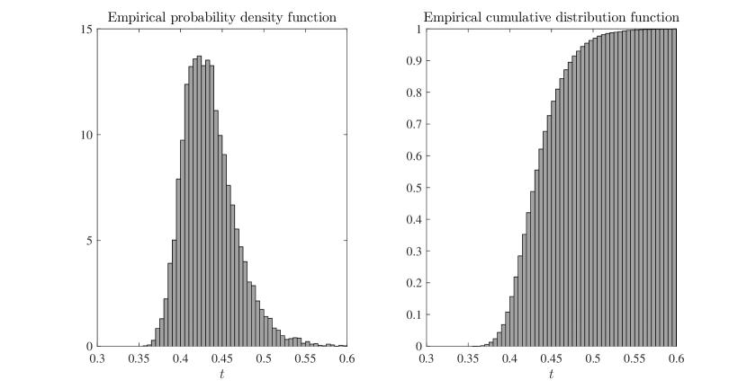
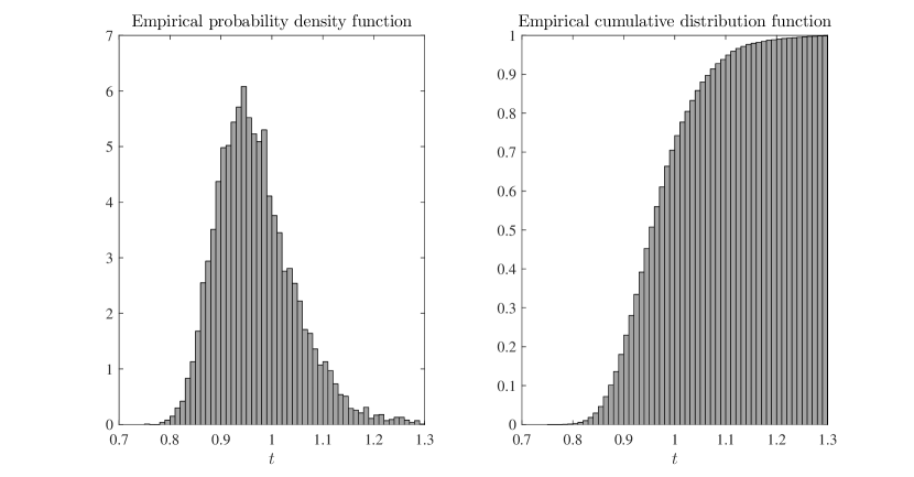
In the second experiment we derived empirical distribution of the restricted isometry constant δssubscript𝛿𝑠\delta_{s} for quaternion Gaussian random matrices and compared it with the case of real Gaussian random matrices. We carried out the simulations for matrices 𝚽𝕂m×n𝚽superscript𝕂𝑚𝑛\mathbf{\Phi}\in\mathbb{K}^{m\times n}, where 𝕂=𝕂\mathbb{K}=\mathbb{H} or 𝕂=𝕂\mathbb{K}=\mathbb{R}, with parameters n=256𝑛256n=256, m=64𝑚64m=64, and for unit s𝑠s-sparse vectors 𝕩𝕂n𝕩superscript𝕂𝑛\mathbbm{x}\in\mathbb{K}^{n} such that s=m2=32𝑠𝑚232s=\frac{m}{2}=32.

Recall that the s𝑠s-restricted isometry constant can be equivalently defined as

δs=max|𝚽𝕩221|,subscript𝛿𝑠superscriptsubscriptdelimited-∥∥𝚽𝕩221\delta_{s}=\max\left|{\left\lVert{\mathbf{\Phi}\mathbbm{x}}\right\rVert_{2}^{2}-1}\right|,

where the maximum is taken over the set of all s𝑠s-sparse vectors 𝕩𝕂n𝕩superscript𝕂𝑛\mathbbm{x}\in\mathbb{K}^{n} such that 𝕩2=1subscriptdelimited-∥∥𝕩21\left\lVert{\mathbbm{x}}\right\rVert_{2}=1. To estimate the cumulative distribution function of the random variable δssubscript𝛿𝑠\delta_{s} for each random matrix 𝚽𝚽\mathbf{\Phi} we drew 105superscript10510^{5} s𝑠s-sparse unit vectors and took maximum over this set. The matrix sample consisted of 104superscript10410^{4} realizations of the random variable 𝚽𝚽\mathbf{\Phi} in both cases. Entries of the matrices were independently sampled from the normal distribution with mean zero and variance 1m1𝑚\frac{1}{m}, i.e. 𝒩(0,1m)𝒩01𝑚\mathcal{N}\left(0,\frac{1}{m}\right) in the real case and 𝒩(0,1m)subscript𝒩01𝑚\mathcal{N}_{\mathbb{H}}\left(0,\frac{1}{m}\right) in the quaternion case.

Results of this experiment – for real and quaternion random matrices – are shown in Fig. 3 and Fig. 4 respectively. In view of the previous theoretical considerations, we can see that (with certain probability) the s𝑠s-restricted isometry constant of a quaternion Gaussian random matrix is small. It proves, in particular, that there exist quaternion matrices satisfying the RIP. Moreover, notice that the s𝑠s-restricted isometry constant of a quaternion random matrix 𝚽m×n𝚽superscript𝑚𝑛\mathbf{\Phi}\in\mathbb{H}^{m\times n} is statistically smaller than its real counterpart for a matrix 𝚽m×n𝚽superscript𝑚𝑛\mathbf{\Phi}\in\mathbb{R}^{m\times n} of the same size. As we previously mentioned, we think that the reason for this phenomenon is smaller variance of the Rayleigh random variable in the quaternion case (Lemma 3.1).
Refer to caption

(a)

(b)

Figure 3: Empirical distributions of δssubscript𝛿𝑠\delta_{s} for Gaussian random matrices 𝚽m×n𝚽superscript𝑚𝑛\mathbf{\Phi}\in\mathbb{R}^{m\times n}, n=256𝑛256n=256, m=64𝑚64m=64, s=32𝑠32s=32.

Refer to caption

(a)

(b)

Figure 4: Empirical distributions of δssubscript𝛿𝑠\delta_{s} for Gaussian random matrices 𝚽m×n𝚽superscript𝑚𝑛\mathbf{\Phi}\in\mathbb{H}^{m\times n}, n=256𝑛256n=256, m=64𝑚64m=64, s=32𝑠32s=32.

Finally, one might be interested in comparing these results with the formulation of Theorem 4.2. We should remember, however, that the estimate in this theorem is significant only for very large n𝑛n (more than few thousand) and snmuch-less-than𝑠𝑛s\ll n (in practice, less than a dozen) and in our experiment, due to computational reasons, n=256𝑛256n=256 and s=32𝑠32s=32. As we also commented, we are aware that this result is not sharp and the numerical experiment additionally suggests that it can be improved in future.

6 Conclusion

This article brings positive answer to the question about existence of quaternion matrices satisfying the RIP. We confirm that – as it was conjectured – restricted isometry constants of Gaussian quaternion matrices are small with big probability (and typically smaller than their real counterparts). Together with our previous result, in which we proved that quaternion measurement matrices with small RIP constants allow exact reconstruction of sparse quaternion vectors, it explains success of compressed sensing based experiments in the quaternion algebra and brings hope for their wider applications.

The main result, however, in the current form is not sharp. One of the reasons is that we used techniques previously applied to the case of real subgaussian random matrices. It would be interesting in the future to study distribution of singular values of quaternion Gaussian matrices in order to improve our result. Other direction of the further research might be search for other quaternion matrices satisfying the RIP, in particular, those more desired from the application point of view, e.g. partial quaternion DFT matrix.


Acknowledgments

The research was supported in part by WUT grant No. 504/02499/1120. The work conducted by the second author was supported by a scholarship from Fundacja Wspierania Rozwoju Radiokomunikacji i Technik Multimedialnych.


References

  • [1] A. Badeńska, Ł. Błaszczyk, Compressed sensing for real measurements of quaternion signals, preprint (2015), arXiv:1605.07985.
  • [2] A. Badeńska, Ł. Błaszczyk, Compressed sensing in the quaternion algebra, preprint (2017), arXiv:1704.08202.
  • [3] Q. Barthélemy, A. Larue, J. Mars, Color Sparse Representations for Image Processing: Review, Models, and Prospects, IEEE Trans Image Process, (2015), 1–12.
  • [4] E. J. Candès, T. Tao, Decoding by linear programming, IEEE Trans. Inform. Theory 51 (12) (2005) 4203–4215.
  • [5] S. Foucart, H. Rauhut, A mathematical introduction to compressive sensing, Applied and Numerical Harmonic Analysis, Birkhäuser/Springer, New York (2013).
  • [6] N. Gomes, S. Hartmann, U. Kähler, Compressed Sensing for Quaternionic Signals, Complex Anal. Oper. Theory 11 (2017), 417–455.
  • [7] M. B. Hawes, W. Liu, A Quaternion-Valued Reweighted Minimisation Approach to Sparse Vector Sensor Array Design, Proceedings of the 19th International Conference on Digital Signal Processing, (2014), 426–430.
  • [8] O. James, H.-N. Lee, Restricted Isometry Random Variables: Probability Distributions, RIC Prediction and Phase Transition Analysis for Gaussian Encoders, preprint (2015), arXiv:1410.1956v4.
  • [9] O. James, On the RIP of Real and Complex Gaussian Sensing Matrices via RIV framework in Sparse Signal Recovery Analysis, IEEE sponsored 2nd International Conference on Electronics and Communications System (2015).
  • [10] O. James, Revisiting the RIP of Real and Complex Gaussian Sensing Matrices Through RIV Framework, Wireless Pers Commun, 87 (2016), no. 2, 513–526.
  • [11] D. R. Jensen, A note on positive dependence and the structure of bivariate distributions, SIAM J. Appl. Math. 20 (1971), 749–753.
  • [12] N. Le Bihan, The geometry of proper quaternion random variables, Signal Processing 138 (2017), 106–116.
  • [13] T. Royen, Some probability inequalities for multivariate gamma and normal distributions, Far East J. Theor. Stat. 51 (2015), no. 1-2, 17–36.
  • [14] J. F. Sturm, Using SeDuMi 1.02, A Matlab toolbox for optimization over symmetric cones, Optimization Methods and Software 11 (1999), no. 1-4, 625–653.
  • [15] N. N. Vakhania, G. Z. Chelidze, Quaternion Gaussian random variables, (Russian) Teor. Veroyatn. Primen. 54 (2009), no. 2, 337–344; translation in Theory Probab. Appl. 54 (2010), no. 2, 363–369.
  • [16] M. Wainwright, Basic tail and concentration bounds, High-dimmensional statistics: A non-asymptotic viewpoint (Ed. M. Wainwright), manuscript (2016(.
  • [17] J. Wu, X. Zhang, X. Wang, L. Senhadji, H. Shu, L1-norm minimization for quaternion signals, Journal of Southeast University 1 (2013) 33–37.