Transverse parton momenta in single inclusive hadron production in ${e^{+}}{e^{-}}$ annihilation processes.

Abstract

We study the transverse momentum distributions of single inclusive hadron production in ${e^{+}}{e^{-}}$ annihilation processes. Although the only available experimental data are scarce and quite old, we find that the fundamental features of transverse momentum dependent (TMD) evolution, historically addressed in Drell-Yan processes and, more recently, in Semi-inclusive deep inelastic scattering processes, are visible in ${e^{+}}{e^{-}}$ annihilations as well. Interesting effects related to its non-perturbative regime can be observed.
We test two different parameterizations for the $p_{\perp}$ dependence of the cross section: the usual Gaussian distribution and a power-law model. We find the latter to be more appropriate in describing this particular set of experimental data, over a relatively large range of $p_{\perp}$ values. We use this model to map some of the features of the data within the framework of TMD evolution, and discuss the caveats of this and other possible interpretations, related to the one-dimensional nature of the available experimental data.

1 Introduction

Transverse momentum dependent distribution and fragmentation functions (TMDs) are fundamental tools to understand the structure of nucleons in terms of their elementary constituents, quarks and gluons. TMDs are non-perturbative quantities which embed important correlations among partonic and hadronic intrinsic properties, like spin or orbital angular momentum, and their internal transverse motion.

TMD parton distribution functions can be interpreted, at leading twist, as number densities of partons carrying a light-cone momentum fraction $x$ of the parent nucleon momentum $P$. Unpolarized and polarized TMD distribution functions have extensively been studied in Drell-Yan processes and semi-inclusive deep inelastic scattering (SIDIS) in the past; new-generation, dedicated experiments are currently running (like Drell-Yan at COMPASS or at RHIC) or are being planned (like the Electron-Ion Collider in the US and the AFTER proposal at CERN-LHC).

Of equal importance are the TMD fragmentation functions, which embed fundamental information on the hadronization process, where a hadron $h$, carrying a light-cone fraction $z$ of the fragmenting parent parton, is produced. TMD fragmentation functions can be measured in single- or double-inclusive hadron production in $e^{+}e^{-}$ annihilation processes or, in a more involved way, in SIDIS, where they necessarily couple to a TMD distribution function. Even with the best SIDIS data presently available, several complications remain to be solved. Extensive recent studies can be found, for example, in Refs. [1, 2, 3, 4, 5]

In $e^{+}e^{-}$ collisions, at c.m. energies below the $Z^{0}$ mass, the electron and positron predominantly annihilate to form a single virtual photon, which can subsequently produce a $q\bar{q}$ pair. The quark and anti-quark will then convert into hadrons. At sufficiently high energies, these multi-hadronic events are expected to form two back-to-back jets (due to the limited transverse momentum along the original quark direction). Single inclusive distributions in variables relative to the jet direction, which is expected to be the quark direction, will therefore give information about the fragmentation of quarks into hadrons. In particular, the dependence of the inclusive distributions in momentum transverse to the jet axis will provide the $golden\;channel$ toward the phenomenological extraction of TMD FFs. An illustration of this process is given in Figure 1.

While much effort has been put into measuring and extracting unpolarized and even polarized TMD PDFs (the Sivers function is a well-known example), little or no experimental information on TMD FFs is presently available. BELLE and BaBar Collaborations have recently presented new multi-dimensional data analyses of the Collins asymmetry in $e^{+}e^{-}\to h_{1}\,h_{2}\,X$ processes, which have allowed a first glance to the intrinsic transverse motion of partons inside hadrons through the extraction of the Collins function, a polarized, chirally-odd TMD fragmentation function. Relevant recent literature on this and other $e^{+}e^{-}$ related subjects are presented in Refs. [6, 7, 8, 9]. However, no modern measurements exist of the unpolarized TMD FFs, although a thorough knowledge of this function would be of fundamental importance for any TMD study.

While waiting for up-to-date, high statistics and (possibly) multidimensional results on the $p_{\perp}$ distribution of $e^{+}e^{-}$ unpolarized cross sections (the BELLE Collaboration has already presented some of their preliminary Monte Carlo simulations at SPIN 2016 [10]), we concentrate on a set of rather old measurements of single inclusive hadron production in $e^{+}e^{-}$ annihilation processes, $e^{+}e^{-}\to h\,X$, by the TASSO Collaboration at PETRA (DESY) [11, 12]: $p_{\perp}$ distributions were provided for four different c.m. energies between 14 and 44 GeV, corresponding to charged particle production summed over all charges and all particle species, with no flavor separation. Cross sections are given as functions of $p_{\perp}$, integrated over the energy fraction $z_{h}=2E_{h}/\sqrt{s}$ of the detected hadron $h$. Note that, up to corrections of order $p_{\perp}^{2}/s$, $z_{h}$ coincides with the light-cone momentum fraction $z$. Although no information is offered about possible cuts applied to $z_{h}$, average values are provided for each c.m. energy set, as summarized in Table 1: they correspond to rather low values, ranging from $\langle z_{h}\rangle$ = 0.13 at 14 Gev to $\langle z_{h}\rangle$ = 0.08 at 44 GeV. Together with TASSO data, we also consider the analogous MARKII Collaboration measurements [13], collected at the SLAC storage ring PEP, at a fixed c.m. energy of 29 GeV, and PLUTO data on the average transverse momentum square [14], collected at PETRA (DESY).

Crucial to all these data is the correct determination of the jet axis, to which the $p_{\perp}$ distributions are most sensitive, beside proper treatment of geometric acceptance effects, trigger bias, kinematics cuts and radiative corrections. These corrections, obtained by comparison to Monte Carlo simulations, are somehow model dependent. Clearly all these issues introduce very large uncertainties which, according to modern standards, were largely underestimated.

Figure 1: Illustration of a typical hadronic event from the $e^{+}e^{-}$ annihilation process, showing the reconstructed jet axis, the hadron momentum $P_{h}$ and its transverse component $p_{\perp}$, perpendicular to the jet axis.

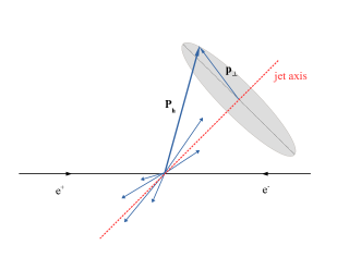
Although these data are affected by several limitations (no hadron separation, limited coverage, $z_{h}$ integration, difficulties in reconstructing the jet axis, etc), they represent an extremely interesting example of a direct measurement of intrinsic transverse momenta. In fact, as mentioned above, the jet axis resulting from each $e^{+}e^{-}$ scattering identifies the direction of the fragmenting $q\bar{q}$ pair ($q$ and $\bar{q}$ should be back to back in the $e^{+}e^{-}$ c.m. frame if radiative effects are appropriately subtracted), and the detected $p_{\perp}$ represents a direct measurement of the transverse momentum of the final hadron with respect to the fragmenting parent parton, see Figure 1.

The purpose of this article is two-folded: first, we will devise and test an appropriate functional form to describe the $p_{\perp}$ distributions measured by TASSO and MARKII, achieving as much information as we possibly can on the TMD unpolarized FF; then, a careful interpretation of our results will be provided focusing on the features related to TMD factorization within a TMD evolution scheme, in the non-perturbative regime.

As these measurements offer quite limited information, we will not be able to perform a detailed extraction of the TMD fragmentation functions as done in the past [15, 16, 17, 2, 8]. However, we will observe that interesting signatures of TMD factorization in the non perturbative regime can be detected in these data sets. In particular, we will find indications that a power-law $p_{\perp}$ behavior, different from the Gaussian parametrization of the TMD FFs we usually used in our previous analyses, might reproduce these data more successfully, especially as $p_{\perp}$ grows larger then a few hundred MeV and we enter the region in which TMD evolution effects start to become more visible.

Experiment	c.m. energy	$\langle z_{h}\rangle$
TASSO	14 GeV	0.13
	22 GeV	0.11
	35 GeV	0.09
	44 GeV	0.08
MARK II	29 GeV	0.09
PLUTO	7.7 GeV	–
	9.4 GeV	–
	12.0 GeV	–
	13.0 GeV	–
	17.0 GeV	–
	22.0 GeV	–
	27.6 GeV	–

Table 1: Upper and central panels: center of mass energies and corresponding $z_{h}$ mean values for the TASSO and MARK II cross sections. Lower panel: center of mass energies corresponding to PLUTO measurements of $\langle p_{\perp}^{2}\rangle$.

2 Formalism

Similarly to the collinear case [18], the ${e^{+}}{e^{-}}\to hX$ cross section can be casted in the following form:

$$\frac{d\sigma^{h}}{dz\,d^{2}\mbox{\boldmath$p$}_{\perp}}=L_{\mu\nu}W^{\mu\nu}=\frac{4\pi\alpha^{2}}{3s}\,z\,F_{1}^{h}(z,p_{\perp};Q^{2})\,.$$ (1)

Within TMD-factorization, up to power suppressed terms, the hadronic tensor $W$ can be expressed as

$$W^{\mu\nu}=W^{\mu\nu}_{TMD}+W^{\mu\nu}_{coll}\;.$$ (2)

The first term on the right hand side of Eq. (2), $W^{\mu\nu}_{TMD}$, corresponds to the region of small transverse momenta, while the second, $W^{\mu\nu}_{coll}$, is calculable within collinear factorization and contains corrections that become important at larger values of $p_{\perp}$. In the case at hand, as there is only one observed final hadron, one may write for the TMD term:

$$W^{\mu\nu}_{TMD}\propto\sum_{f}|{\cal H}_{f}(Q;\mu)|^{\mu\nu}D_{h/f}(z,\mbox{\boldmath$p$}_{\perp};\mu,\zeta_{D}),$$ (3)

where $Q$ is the hard scale of the process, $z$ and $\mbox{\boldmath$p$}_{\perp}$ are the observed hadronic variables, $\mu$ is the renormalization scale, while $\zeta_{D}$ is a regulator for the light-cone divergences that arise in TMD-factorization. The hard factor ${\cal H}_{f}$ can be calculated in perturbation theory, while the TMD FF is defined by the relations

$$D_{h/f}(z,z\mbox{\boldmath$k$}_{\perp};\mu,\zeta_{D})\equiv\frac{1}{(2\pi)^{2}}\int d^{2}\mbox{\boldmath$b$}_{\perp}e^{-i\mbox{\boldmath$k$}_{\perp}\cdot\,\mbox{\boldmath$b$}_{\perp}}\tilde{D}_{h/f}(z,\mbox{\boldmath$b$}_{\perp};\mu,\zeta_{D})\,,$$ (4)

$$\tilde{D}_{h/f}(z,\mbox{\boldmath$b$}_{\perp};\mu,\zeta_{D})\equiv$$

$$\;\sum_{j}\Bigg{[}\tilde{C}_{j/f}\otimes d_{h/j}(z;\mu_{b})/z^{2}\Bigg{]}$$

$$\times\,{\rm exp}\Bigg{\{}\int_{\mu_{b}}^{\mu}\frac{d\tilde{\mu}}{\tilde{\mu}}\Big{[}\gamma_{D}(\alpha_{s}(\tilde{\mu});1)-\gamma_{K}(\alpha_{s}(\tilde{\mu}))\log\left(\frac{\zeta_{D}}{\tilde{\mu}}\right)\Big{]}\Bigg{\}}$$

$$\times\,{\rm exp}\Bigg{\{}\tilde{K}(b_{*};\mu_{b})\log\left(\frac{\zeta_{D}}{\mu_{b}}\right)\Bigg{\}}$$

$$\times\,{\rm exp}\Bigg{\{}g_{h/j}(z,b_{\perp})+g_{K}(b_{\perp})\log\left(\sqrt{\frac{\zeta_{D}}{\zeta_{D}^{(0)}}}\right)\Bigg{\}}\,.\hphantom{qqqqq}$$ (5)

Notice the conjugate variable to $\mbox{\boldmath$b$}_{\perp}$ is $\mbox{\boldmath$k$}_{\perp}$ rather than $\mbox{\boldmath$p$}_{\perp}$ ($\mbox{\boldmath$k$}_{\perp}$ is the component of the fragmenting parton momentum transverse to the final hadron, in a reference frame in which the latter is purely longitudinal). Details on the various ingredients of Eq. (5) can be found in Refs. [18, 19]. For our purposes it suffices to note that in the first three factors of Eq. (5) all the ingredients are calculable within perturbation theory, except for the collinear fragmentation function $d_{h/j}$. Notice that the Wilson coefficients, $\tilde{C}_{j/f}$, the integral of the anomalous dimensions, $\gamma_{D}$ and $\gamma_{K}$, and the the Collins-Soper (CS) kernel, $\tilde{K}$, depend on $b_{\perp}$ only through the quantity $b_{*}$, which is set to remain smaller than some maximum $b_{max}$. The last factor in Eq. (5) contains only non-perturbative information.

There is some freedom in the definition of Eq. (5), encompassed in the arbitrary quantities $\mu$, $\mu_{b}$, $b_{*}$, $\zeta_{D}$, $\zeta_{D}^{(0)}$. For our analysis we adopt the usual choices [19], $\mu\to Q$, $\zeta_{D}\to Q^{2}$ and $\mu_{b}=2e^{-\gamma_{E}}/b_{*}$, where $\gamma_{E}$ is the Euler-Mascheroni constant. With these choices the CS kernel $\tilde{K}$ vanishes at order $\alpha_{s}$, so the third factor in Eq. (5) reduces to one. To this same order, the factor containing the anomalous dimensions $\gamma_{D}$ and $\gamma_{K}$ can be expressed in a closed analytic form. For our purposes, it will be useful to classify the result of this integral in terms of its dependencies on $Q$ and $b_{*}$, namely

$${\rm exp}\Bigg{\{}\int_{\mu_{b}}^{\mu}\frac{d\tilde{\mu}}{\tilde{\mu}}\Big{[}\gamma_{D}(g(\tilde{\mu});1)-\gamma_{K}(g(\tilde{\mu}))\log\left(\frac{\zeta_{D}}{\tilde{\mu}}\right)\Big{]}\Bigg{\}}$$

$$\longrightarrow{\cal N}_{\Gamma}(Q)\,f_{\;\Gamma}(b_{*},Q_{0})\,\exp\Bigg{\{}\lambda_{\Gamma}(b_{*})\log\left(\frac{Q}{Q_{0}}\right)\Bigg{\}}\,,$$ (6)

for which we have used the results of the Appendices in Ref. [3]. The quantities ${\cal N}_{\Gamma}(Q)$, $f_{\;\Gamma}(b_{*},Q_{0})$ and $\lambda_{\Gamma}(b_{*})$ are flavor independent functions that encode the most prominent perturbative effects in the definition of the TMD FF. The last of these three functions,

$$\lambda_{\Gamma}(b_{*})\equiv\frac{32}{27}\log\left(\log\frac{2e^{-\gamma_{E}}}{\Lambda_{QCD}\;b_{*}}\right)\,,$$ (7)

is the most interesting since it correlates $b_{*}$ with $Q$, which means it has the effect of modifying the shape of the TMD FF under evolution. With these considerations, one may write for the TMD FF:

$$\tilde{D}_{h/f}(z,\mbox{\boldmath$b$}_{\perp};\mu,\zeta_{D})=$$

$${\cal N}_{\Gamma}(Q)\sum_{j}\Bigg{[}\tilde{C}_{j/f} \otimes d_{h/j}(z;\mu_{b})/z^{2}\Bigg{]}e^{g_{h/j}(z,b_{\perp})}\,f_{\;\Gamma}(b_{*},Q_{0})$$

$$\times\exp\Bigg{\{}\Big{(} \lambda_{\Gamma}(b_{*})+g_{K}(b_{\perp})\Big{)}\log\left(\frac{Q}{Q_{0}}\right)\Bigg{\}}\,.$$ (8)

Therefore, except for the overall normalization factor ${\cal N}_{\Gamma}(Q)$, the effects of evolution at order $\alpha_{s}$ can be mapped to either the non-perturbative function $g_{K}(b_{\perp})$, or the perturbative quantity $\lambda_{\Gamma}(b_{*})$.

In the region where TMD effects dominate (see Eqs. (1)-(3)), flavor independence of $g_{K}$ and $\lambda_{\Gamma}$ in Eq. (2) implies

$${\cal F}^{-1}\left\{\frac{d\sigma^{h}}{dz\,d^{2}\mbox{\boldmath$p$}_{\perp}}\right\}\propto\, \exp\Bigg{\{}\Big{(}\lambda_{\Gamma}(b_{*})+g_{K}(b_{\perp})\Big{)}\log\left(\frac{Q}{Q_{0}}\right)\Bigg{\}}\,\Bigg{|}_{b_{\perp}\to z\;b_{\perp}}\,,$$ (9)

where the symbol ${\cal F}^{-1}$ indicates the two-dimensional inverse Fourier transform, from momentum to impact parameter space, and the transformation $b_{\perp}\to z\;b_{\perp}$ is needed to account for the extra factor of $z$ that appears in the definition of Eq. (3), compared to the TMD term in the hadronic tensor in Eq. (2). In the following section we will use relations (7)-(9) to make an interpretation of our results.

3 Data fitting and results

A full analysis within a TMD-evolution scheme should include all of the contributions in Eq. (2), as well as a matching prescription to interpolate between regions of small and large $p_{\perp}$, as originally prescribed in Ref. [20]. It is important to stress that all of these ingredients provide crucial constraints that any full analysis should include. Some recent studies related to the complications involved in the matching prescriptions for SIDIS processes are presented in Refs. [21, 4]. However, for such type of analyses, multidimensional data sets are most suitable, where one can completely disentangle the effects of different kinematics variables. In the case of the measurements of Ref. [11, 12, 13, 14], the large systematic uncertainties induced by $z$-integration can only render limited insight on TMD-effects. However, it is still interesting to investigate what information about evolution can be extracted from these measurements. In fact, even for these $z$-integrated cross sections, one may expect the shape of the $p_{\perp}$ distributions to be affected by TMD-evolution effects.

In order to address this question it becomes essential to make an estimate of where the large transverse momentum corrections start becoming important in the TASSO and MARKII data sets. To do so, we start by considering the errors of the TMD approximation, which are of order ${\cal O}(k_{\perp}/Q)={\cal O}(p_{\perp}/zQ)$. In general, one expects that at $p_{\perp}\sim zQ$, the cross section should receive contributions from the collinear term in Eq. (2). Using the average values of Table 1, one may estimate that this contributions should be significant at $p_{\perp}\sim 2\,{\rm GeV}$. We identify this as the matching region. In this article we will attempt to extract information only about the non-perturbative evolution carried by $g_{K}$ in Eq. (2), so we will constrain our analysis to the region of $p_{\perp}<1.0\;{\rm GeV}$. Note that we also impose a lower cut on $p_{\perp}$, such that $p_{\perp}>0.03$ GeV; this amounts to excluding the first data point in the TASSO data sets.

In order to relate the shape of the data to possible TMD-evolution effects, one needs a model that can reproduce the transverse momentum distribution of the final hadron $h$. Then, by looking at the $b_{\perp}$-space, one may connect the parameters of the model to some of the information contained in the definition of Eq. (5), as discussed in Ref. [3].

At least two functional forms have been shown to appropriately describe transverse momentum distributions [3, 2].

• Gaussian form: it is the most commonly used parametrization for phenomenological studies, it has been shown to reproduce experimental data very successfully in both Drell-Yan and SIDIS processes. It has the advantage of being easy to integrate analytically.

• Power-law: it is very flexible, even with a limited number of free parameters. Not only can it appropriately reproduce the behavior of the cross section at small $p_{\perp}$, but it can also incorporate its tail at larger $p_{\perp}$ values.

We will consider both of these functional forms in order to describe the low-$p_{\perp}$ region of the data. Our aim is to focus on the kinematics ranges where TMD-effects are dominant. As discussed above, one may estimate that perturbative effects will start to become important roughly around $p_{\perp}\sim 2\,{\rm GeV}$, but could in fact be non-negligible at even smaller values of transverse momentum, especially as the data we consider are integrated over $z$. Our working hypothesis is that for $p_{\perp}<1\;{\rm GeV}$ the TMD-term in Eq. (2) is the largest contribution to the cross section.

We model the structure function $F_{1}$ in Eq. (1) so that

$$\frac{d\sigma^{h}}{dz\,d^{2}\mbox{\boldmath$p$}_{\perp}} = \frac{4\pi\alpha^{2}}{3s}\sum\limits_{q}{{e_{q}}^{2}}\,D_{q}^{h}(z,{p_{\perp}};{Q^{2}})$$ (10)

$$= \frac{4\pi\alpha^{2}}{3s}\sum\limits_{q}{{e_{q}}^{2}}\,D_{q}^{h}(z,Q^{2})\;h(p_{\perp})\,,$$

which extends the leading order expression for the collinear cross section. In Eq. (10), the sum runs over all $q$ and $\bar{q}$ flavors, and we have assumed that the TMD fragmentation function may be written as

$$D_{q}^{h}(z,{p_{\perp}})=D_{q}^{h}(z)\;h(p_{\perp})\,,$$ (11)

where $D_{q}^{h}(z)$ is the collinear, unpolarized FF (which we take from Ref. [22]). The function $h(p_{\perp})$ incorporates all of the $p_{\perp}$ dependence of the TMD FF, it is flavor independent and it is normalized so that it integrates to unity.

The TASSO collaboration provides cross sections differential in $p_{\perp}$, normalized to the fully inclusive cross section, which at leading order read

$$\sigma_{tot}\overset{LO}{=}\sigma_{0}=\frac{4\pi\alpha^{2}}{3s}\,\sum_{q}{{e_{q}}^{2}},$$ (12)

so that our fits will involve the expression

$$\frac{1}{\sigma_{0}}\frac{d\sigma^{h}}{dp_{\perp}}=2\pi p_{\perp}\left[\int\!\!dz\,\frac{\sum_{q}e_{q}^{2}\,D_{q}^{h}(z;Q^{2})}{\sum_{q}e_{q}^{2}}\right]h(p_{\perp})\,.$$ (13)

A note of caution is necessary at this point. The TASSO distributions in $p_{\perp}$ at different energies cannot be described by simply using the model of Eq. (13). Instead, one must incorporate a treatment for their normalizations at different values of $Q$. While this may be in conflict with a possible probabilistic interpretation of the function $h(p_{\perp})$, it should not affect our conclusions regarding TMD evolution, since for that, we will focus on aspects of the $p_{\perp}$ distributions that regard their shape, but not the precise values of their maxima. We note that accounting for all the features of these data may be challenging even within a full TMD analysis, as large systematic errors may translate into out-of-control normalizations when dealing with $z$-integrated data.

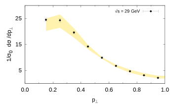
The fits in the next subsections are performed on the TASSO $p_{\perp}$-distributions only. We will use the MARK II $p_{\perp}$-dependent normalized cross section and the PLUTO measurements of $\langle p_{\perp}^{2}\rangle$ to cross-check our results. When appropriate, error bands corresponding to a $2\sigma$ confidence level are provided, obtained by generating random points in the parameter space for which $\chi_{i}^{2}\in[\chi_{0}^{2},\chi_{0}^{2}+\Delta\chi^{2}]$, where $\chi_{0}^{2}$ is the minimal value given by the fit and $\Delta\chi^{2}$ depends on the number of parameters of the model; the relevant cases in our fits involve either $6$ or $7$ free parameters, which correspond to $\Delta\chi^{2}$ values of $12.85$ and $14.34$, respectively.

3.1 Gaussian shape at low $p_{\perp}$

We start by applying a Gaussian model with a constant width:

$$h(p_{\perp})=\frac{{e^{-{p_{\perp}}^{2}/\langle{{p_{\perp}}^{2}}\rangle}}}{{\pi\langle{{p_{\perp}}^{2}}\rangle}}\,.$$ (14)

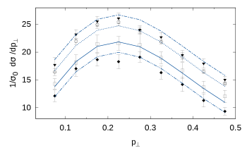
As mentioned earlier, in order to describe the data we need an appropriate treatment for the normalization. Unexpectedly, we find that using different multiplicative constants, one for each energy, is not enough to obtain a good fit, even in the limited region of $p_{\perp}<0.5$ GeV (see the first entry in Table 2). Instead, by also introducing a $Q$-dependent shift for the cross sections, so that one has

$$N\;\frac{1}{\sigma_{0}}\frac{{d{\sigma^{h}}}}{{dz\,{d^{2}}{{\bf p}_{\perp}}}}+\delta\,Q\,,$$ (15)

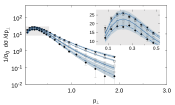
one can obtain a good description of the data, as seen in the second entry of Table 2 and on the upper panel of Figure 2. This unconventional prescription to deal with the normalization, while leaving little room for a partonic interpretation for the function $h(p_{\perp})$, allows us to verify quantitatively that as far as the width of the $p_{\perp}$ distribution is concerned, no significant change can be observed with growing Q. One may not conclude, however, that TMD-effects do not appear in these transverse momentum ranges, but rather that the data analyzed do not have the necessary accuracy to show possible width changes in this region. Thus, one must try to extend the description of the data to larger values of $p_{\perp}$.

Figure 2: Gaussian description of the TASSO $p_{\perp}$ distributions at 4 different c.m. energies [12]. On the upper panel the Gaussian model with constant width, see Eqs. (14) and (15), up to $p_{\perp}=0.5$ GeV. On the lower panel the Gaussian model with the Q dependent width of Eq. (16), up to $p_{\perp}=1.0$ GeV.

Parametrization	Normalization	Gaussian width	$\chi^{2}_{pt}$
Gaussian - I	$N=\{N_{14},N_{22},N_{35},N_{44}\}$	$\langle p_{\perp}^{2}\rangle=$ constant
$p_{\perp}\in[0.03-0.50]$ GeV	$N_{14}=2.3\pm 0.2$,     $N_{22}=2.7\pm 0.2$	$\langle p_{\perp}^{2}\rangle=0.118\pm 0.004$ GeV2	5.9
36 data points	$N_{35}=3.1\pm 0.1$,     $N_{44}=3.2\pm 0.1$
Gaussian - II	$N$, $\delta\,Q$	$\langle p_{\perp}^{2}\rangle=$ constant
$p_{\perp}\in[0.03-0.50]$ GeV	$N=1.8\pm 0.2$	$\langle p_{\perp}^{2}\rangle=0.098\pm 0.005$ GeV2	0.74
36 data points	$\delta=0.22\pm 0.03$
Gaussian - III	$N=\{N_{14},N_{22},N_{35},N_{44}\}$	$\langle p_{\perp}^{2}\rangle=2g_{1}+2g_{2}z^{2}\log\frac{Q}{3.2}$
$p_{\perp}\in[0.03-1.00]$ GeV	$N_{14}=2.7\pm 0.2$,    $N_{22}=3.3\pm 0.3$	$g_{1}=0.013\pm 0.004$ GeV2	2.7
56 data points	$N_{35}=4.0\pm 0.1$,    $N_{44}=4.3\pm 0.2$	$g_{2}=2.6\pm 0.3$ GeV2

Table 2: Fits of the TASSO four sets of cross sections, corresponding to the Gaussian parameterization of the $p_{\perp}$ distributions. Parametrization I refers to the usual choice of Eq. (14), Parametrization II refers to the Gaussian corrected by a Q-dependent shift, see Eq. (15), while Parametrization III corresponds to a Gaussian distribution with a Q dependent width, as in Eq. (16).

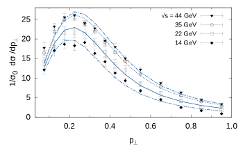
For $p_{\perp}>0.5\,{\rm GeV}$, a noticeable dependence of the distributions on the c.m energy suggests that a $Q$-dependent width may be appropriate. However, even with this extension of the model, describing the data past this point turns out to be extremely difficult. To illustrate this, we consider the functional form

$$\langle p_{\perp}^{2}\rangle=2\,g_{1}+2\,g_{2}\;z^{2}\log\left(\frac{Q}{2\,Q_{0}}\right)\,,$$ (16)

which allows for some comparison to previous phenomenological studies [23, 24] where, within a CSS evolution scheme, a Gaussian behavior of the non-perturbative Sudakov factor in the $b_{\perp}$ space was assumed. This time, we use a multiplicative constant for each value of $Q$ ($\delta=0$ in Eq. (15)), and fix $Q_{0}=1.6\,{\rm GeV}$. The last entry of Table 2 shows the results of the fit for $p_{\perp}<1\,{\rm GeV}$, using the extended Gaussian model corresponding to Eq. (16). The obtained minimal $\chi^{2}$ value points to a rather low quality of the description of the data. The corresponding plot, in the lower panel of Figure 2, shows that there is some tension between a successful description of the peak at low $p_{\perp}$ and an equally good description of the tail at larger $p_{\perp}$ values. As we will show in the next subsection, the power-law can in fact accommodate for both of these features of the data.

3.2 Power-law shape at low and moderate $p_{\perp}$

So far, we have tried the Gaussian ansatz for the $p_{\perp}$ distributions. We have found that the data favors a constant width, for values up to $p_{\perp}=0.5\,{\rm GeV}$. However, this can only be achieved by introducing a $Q$-dependent shift, which cannot be easily interpreted within a partonic picture. The Gaussian class of models does not seem to be appropriate for larger values of $p_{\perp}$.

In order to describe the data up to $p_{\perp}=1\,{\rm GeV}$, we test a power-law parametrization, given by

$$h(p_{\perp})=2(\alpha-1)\mbox{\small M}^{2\;(\alpha-1)}\frac{1}{\left(p_{\perp}^{2}+\mbox{\small M}^{2}\right)^{\alpha}}\,,$$ (17)

where the factor $2(\alpha-1)\mbox{\small M}^{2\;(\alpha-1)}$ is set so that $h(p_{\perp})$ integrates to unity. The two-dimensional inverse Fourier transform of this function has an exponentially decaying asymptotic behavior, consistent with what would be expected from general arguments within quantum field theory, as discussed in Refs. [18, 25]. In impact parameter space the power-law becomes

$${\cal F}^{-1} \left\{\frac{1}{\left(p_{\perp}^{2}+\mbox{\small M}^{2}\right)^{\alpha}}\right\}=\frac{1}{2^{\alpha}\,\pi\,\Gamma(\alpha)}\left(\frac{b_{\perp}}{\mbox{\small M}}\right)^{\alpha-1}\!\!\!K_{1-\alpha}(b_{\perp}\mbox{\small M})$$

$$\overset{{\rm large}\,b_{\perp}}{\longrightarrow}\frac{1}{2^{\alpha}\,\pi\,\Gamma(\alpha)}\left(\frac{b_{\perp}}{\mbox{\small M}}\right)^{\alpha-1}\!\!\!\sqrt{\frac{\pi}{2}}\frac{e^{-b_{\perp}\mbox{\scriptsize M}}}{\sqrt{b_{\perp}\mbox{\small M}}}\left[1+{\cal O}\left(\frac{1}{b_{\perp}\mbox{\small M}}\right)\right]\,,$$ (18)

where $K_{1-\alpha}(b_{\perp}\mbox{\small M})$ is the modified Bessel function of the second kind. In what follows, we use an independent normalization for each value of $Q$. As discussed before, we are interested in the shape of the distributions, rather than on their overall normalizations.

In the power-law parametrization of the $p_{\perp}$-differential cross section, the parameter $\mbox{\small M}^{2}$ is related to the position of its peak, $p_{{}_{\!\!0}}{}_{\!\!{\kern 1.12003pt}\perp}{}$, by the relation $\mbox{\small M}^{2}=\,\big{(}2\,\alpha-1\big{)}p_{{}_{\!\!0}}{}_{\!\!{\kern 1.12003pt}\perp}{}^{\!2}$. Since the studied distributions reach their maximum at roughly the same value of transverse momentum, $p_{\perp}\approx 0.212\,{\rm GeV}$, for all values of the c.m. energy, in our main analysis we have imposed the conditions that

$$\mbox{\small M}^{2}= \,\big{(}2\,\alpha-1\big{)}p_{{}_{\!\!0}}{}_{\!\!{\kern 1.12003pt}\perp}{}^{\!2}$$

$$p_{{}_{\!\!0}}{}_{\!\!{\kern 1.12003pt}\perp}{}= \,0.212\,{\rm GeV}\,.$$ (19)

We have verified that setting $\mbox{\small M}^{2}$ free, does in fact satisfy Eqs. (3.2) within errors. It is, however, useful to reduce the number of parameters by directly imposing these relations.

First, to test that the power-law can appropriately describe the data, we conducted simple independent fits for each value of the c.m. energy, which renders one value of $\alpha$ for each $Q$. The most interesting aspect of this preliminary fit is that it shows a clear dependence of the parameter $\alpha$ on $Q$, despite the use of independent normalizations. The trend of the values for $\alpha$ is displayed in Figure 3, which shows a decrease of the its optimal value with $Q$. Due to the large uncertainties in the determination of $\alpha$, there are likely several functional forms that can accommodate the observed behavior. In order to make an educated guess for a suitable $Q$-dependence in $\alpha$, we assume that the integration over $z$ does not alter the structure of the relation in Eq. (9), namely

$${\cal F}^{-1}\left\{\frac{d\sigma^{h}}{d^{\,2}\mbox{\boldmath$p$}_{\perp}}\right\}\propto \exp\Bigg{\{}\tilde{g}(b_{\perp})\log\left(\frac{Q}{Q_{0}}\right)\Bigg{\}}\,\,,$$ (20)

for some function $\tilde{g}(b_{\perp})$. Thus, one can see that a logarithmic behavior for $\alpha$ may be appropriate by looking at the asymptotic limit of the power-law in $b_{\perp}$-space, Eq. (3.2). First, for the values $\alpha_{0}$ and $\alpha$ that describe the data at two given values $Q_{0}$ and $Q$, if (20) holds, one should have

$$b_{\perp}^{\,\alpha_{0}}\,\exp\Bigg{\{}\tilde{g}(b_{\perp})\log\left(\frac{Q}{Q_{0}}\right)\Bigg{\}}\propto b_{\perp}^{\,\alpha}\,,$$ (21)

in the large-$b_{\perp}$ limit. This can be achieved if

$$\tilde{g}(b_{\perp})\overset{{\rm large}\,\,b_{\perp}}{\longrightarrow}\tilde{\alpha}\log(\nu\,b_{\perp})\,,$$ (22)

for some values $\tilde{\alpha}$ and $\nu$, which in turn provides the relation

$$\alpha=\alpha_{0}+\tilde{\alpha}\log\left(\frac{Q}{Q_{0}}\right)\,.$$ (23)

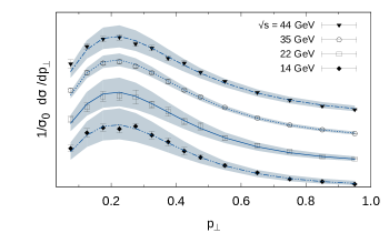
We have implemented Eq. (23) into a fit and confirmed that in fact it reproduces well the TASSO data. Results are shown on the third panel of Table 3, and in the top plot in Figure 4, which includes errors corresponding to a $2\sigma$ confidence level. We compare these results to the MARK II data set in the bottom panel of Figure 4.

The argument presented above, leading to a logarithmic $Q$-dependence for the power $\alpha$, has some caveats. First, it depends on whether Eq. (20) is approximately correct. Furthermore since it considers only the asymptotic large-$b_{\perp}$ behavior of Eq. (3.2), Eq. (23) does not need to hold for values larger than $p_{\perp}\sim\mbox{\small M}$. Therefore, even if one can describe the data, any interpretation of the logarithmic behavior of $\alpha$, in terms of the ingredients that define the TMD FF, Eq. (5), should be taken with great caution. Nonetheless, it is worthwhile to explore this possibility.

Notice that the function $\tilde{g}$ acquires its behavior from $\lambda_{\Gamma}$ and $g_{K}$. Since the first varies slowly with $b_{\perp}$, and in fact does freeze to a constant value at large enough $b_{\perp}$ (see Eq. (7)), one may see Eq. (23) as the manifestation of a logarithmic large-$b_{\perp}$ trend for $g_{k}(b_{\perp})$, analogous to Eq. (22). A behavior consistent with discussions in Refs. [3, 25]. However, we stress that one may well reproduce the data by using different assumptions. As a counter example we consider a simple picture where the cross section takes the form

$$\frac{d\sigma}{dz\,d^{2}\mbox{\boldmath$p$}_{\perp}}\propto\left(\frac{1}{p_{\perp}^{2}+z\,\tilde{\mbox{\small M}}^{2}}\right)^{\,\beta_{1}+\,\beta_{2}\,z}\,,$$ (24)

and where one accounts for the integration over $z$ by some average value $\langle z\rangle$, leading to

$$\frac{d\sigma}{d^{2}\mbox{\boldmath$p$}_{\perp}}\propto\left(\frac{1}{p_{\perp}^{2}+\langle z\rangle\,\tilde{\mbox{\small M}}^{2}}\right)^{\,\beta_{1}+\,\beta_{2}\,\langle z\rangle}\,,$$ (25)

where the parameters $\beta_{1}$, $\beta_{2}$ and $\tilde{\mbox{\small M}}$ are to be determined by a fit. In this case, it is indeed possible to obtain a good description of the data by using the experimental average values of $z$ of Table 1, since they exhibit a seemingly logarithmic trend. However, it is difficult to make a connection to TMD evolution since the values in Table 1 are in general affected by correlations between $Q$ and $z$ of different origin. In fact, notice that the condition of Eq. (3.2) implies a logarithmic behavior for our fit parameter $\mbox{\small M}^{2}$. It is possible that, for instance, the effects of the TMD evolution, encoded in $g_{K}$, result in changes in the power $\alpha$ that fit the data, while the changes in $\mbox{\small M}^{2}$ are the result of correlations induced by the integration over $z$. It seems, however, that the lack of information about the $z$-dependence of the TMD FF in the TASSO and MARK II measurements hinders a more solid conclusion about TMD evolution effects in these data sets.

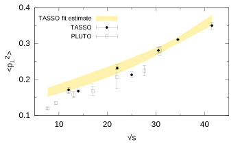
Finally, it is useful to test the model of Eqs. (17) and (23) for larger values of $p_{\perp}$. In fact, this is necessary to calculate $\langle p_{\perp}^{2}\rangle$, since it implies integration over the full range of $p_{\perp}$. For this, we keep the first of the constraints (3.2), but free the parameter $p_{{}_{\!\!0}}{}_{\!\!{\kern 1.12003pt}\perp}{}$. First, we perform a fit including data up to $p_{\perp}=2\,{\rm GeV}$. As seen in Figure 5 and the last entry of Table 3, the model can successfully accommodate this extended range of $p_{\perp}$. This range is, however, not enough to reproduce to a good accuracy the corresponding TASSO measurements of $\langle p_{\perp}^{2}\rangle$. Thus, we further extend the range analysis of TASSO data to values up to $p_{\perp}=3\,{\rm GeV}$ and use the resulting minimal parameters to estimate $\langle p_{\perp}^{2}\rangle$. Figure 6 shows our estimate and the data from TASSO and PLUTO.

Parametrization	Normalization	parameters	$\chi^{2}_{pt}$
	$N=\{N_{14},N_{22},N_{35},N_{44}\}$
Power-law - I	$N_{14}=2.6\pm 0.1$	$\alpha=\{\alpha_{14},\alpha_{22},\alpha_{35},\alpha_{44}\}$	$\chi^{2}_{14}=0.35$
$p_{\perp}\in[0.03-1.00]$ GeV	$N_{22}=3.2\pm 0.2$		$\chi^{2}_{22}=0.30$
$14\times 4$ data point	$N_{35}=4.0\pm 0.1$	$\alpha_{14}=3.3\pm 0.4$,    $\alpha_{22}=2.5\pm 0.3$	$\chi^{2}_{35}=0.88$
	$N_{44}=4.4\pm 0.2$	$\alpha_{35}=2.2\pm 0.1$,    $\alpha_{44}=2.0\pm 0.1$	$\chi^{2}_{14}=0.84$
Power-law - II	$N_{14}=2.6\pm 0.2$	$\alpha$ = constant
$p_{\perp}\in[0.03-1.00]$ GeV	$N_{22}=3.3\pm 0.2$
$56$ data points	$N_{35}=4.0\pm 0.1$	$\alpha=2.2\pm 0.1$	2.87
	$N_{44}=4.2\pm 0.2$
Power-law - III	$N_{14}=2.6\pm 0.2$	$\alpha$ = $\alpha_{0}+\tilde{\alpha}\log(Q/Q_{0})$
$p_{\perp}\in[0.03-1.00]$ GeV	$N_{22}=3.3\pm 0.2$	$Q_{0}=14\,{\rm GeV}$
$56$ data points	$N_{35}=4.0\pm 0.1$		0.66
	$N_{44}=4.4\pm 0.2$	$\alpha_{0}=3.1\pm 0.4$,    $\tilde{\alpha}=-1.0\pm 0.4$
Power-law - IV	$N_{14}=2.6\pm 0.2$	$\alpha$ = $\alpha_{0}+\tilde{\alpha}\log(Q/Q_{0})$
$p_{\perp}\in[0.03-2.00]$	$N_{22}=3.2\pm 0.3$	$Q_{0}=14\,{\rm GeV}$
$76$ data points	$N_{35}=4.0\pm 0.1$	$\alpha_{0}=3.5\pm 0.3$,    $\tilde{\alpha}=-1.1\pm 0.3$	0.95
	$N_{44}=4.3\pm 0.2$	$p_{{}_{\!\!0}}{}_{\!\!{\kern 1.12003pt}\perp}{}=0.219\pm 0.005$

Table 3: Fits of the TASSO four cross sections, corresponding to the power-law parameterization of the $p_{\perp}$ distributions. Parametrization I refers to 4 independent fits (one for each data set corresponding to a different c.m. energy) using the functional form of Eq. (17), with constant $\alpha$ and $\mbox{\small M}^{2}$ parameters. Parametrization II refers to the simultaneous fit of the four data sets, using the functional form of Eq. (17), with constant $\alpha$ and $\mbox{\small M}^{2}$ parameters. Parametrization III refers to the simultaneous fit of the four data sets, using the functional form of Eq. (17), with Q-dependent $\alpha$ and $\mbox{\small M}^{2}$ parameters.

Figure 3: Values of $\alpha$ in Eq. (17) that best describe the distributions of [12]. The triangles represent the minimal values of independent fits, performed for each value of the center of the c.m energy $\sqrt{s}=Q$. The shaded bands indicate the corresponding uncertainty.

Figure 4: In the top panel we show the results from our fit to TASSO experimental data using the power-law of Eqs. (17) and (23), in the range $0.03\,{\rm GeV}<p_{\perp}<1.0\,{\rm GeV}$. To avoid overlapping and provide a clear display of the $2\sigma$ error bands, we plot the distributions for different energies applying an arbitrary shift. In the bottom panel we compare the results from the fit to TASSO data to the MARK II cross section. Note that a different normalization and its uncertainties have to be determined independently for this data set. We dont display the first bin, centered at $p_{\perp}=0.05$ GeV.

Figure 5: Results obtained by using the power-law of Eqs. (17) and (23) compared to TASSO $p_{\perp}$-dependent distributions [12], in the range $0.03\,{\rm GeV}<p_{\perp}<2.0\,{\rm GeV}$. Error bands are computed using a $2\sigma$-confidence level, as explained in Section 3.

Figure 6: Estimation of the transverse momentum mean value, $\langle p_{\perp}^{2}\rangle$, obtained by using the parameters extracted by fitting the TASSO $p_{\perp}$ distributions up to 3.0 GeV. Empty squares correspond to PLUTO data [14] while filled diamonds correspond to TASSO measurements [12]. The shaded area represents the uncertainty of our calculation and is computed as explained in Section 3.

4 Final remarks

TMD FFs embed the essence of hadronization, one of the most important manifestations of QCD in the non-perturbative regime. It is therefore important to gather as much information as possible on these soft quantities, which cannot be computed, but have to be inferred from experiment. Over the last few years, several analyses have been performed to extract the polarized TMD FFs, like the Collins function, using the measurements of the Collins asymmetries in $e^{+}e^{-}\to h_{1}h_{2}X$ processes provided by BELLE and BaBar Collaborations, which delivered multidimensional data (in bins of $z_{1}$, $z_{2}$, $p_{\perp 1}$, $p_{\perp 2}$) with impressive statistics and very high precision. Unfortunately, no analogous data have been provided on the $p_{\perp}$-distributions of the unpolarized cross sections, or multiplicities, to allow for the extraction of the unpolarized TMD FFs. The absence of these fundamental bricks encumbers the analysis of any other polarized, as well as unpolarized, process.

At present, the only available data are some old (and almost forgotten) measurements of $e^{+}e^{-}\to hX$ cross sections from TASSO and MARKII Collaborations. Although these are one-dimensional data and are affected by large uncertainties, as discussed in Section 1, they have the unique advantage of delivering measurements at different c.m. energies; therefore, they can provide a valuable starting point not only to learn about the unpolarized TMD FFs, but also to study the physiognomy of their TMD evolution.

In this article we assess the extent to which the effects of TMD evolution can be observed in these data. For this purpose, our main tool is an analysis based on a simple partonic picture in which the cross section is factorized, as in Refs. [15, 16, 17, 2, 8]. While these types of analysis typically use a Gaussian form, we also test a power-law behavior to describe the data, as suggested in Ref. [3]. We extend this class of models to the case in which the parameterization is supplemented by some Q dependence, and use these results to provide an interpretation within a TMD evolution framework, see Eq. (5), discussing the caveats related to the limited amount of information provided by these data.

We start by modeling the $p_{\perp}$ dependence of the cross section by a Gaussian shape and fit the four sets of TASSO cross section data (corresponding to four different c.m. energies) to extract the corresponding free parameters, see Table 2. Our analysis shows that the Gaussian distribution can only describe the data up to $p_{\perp}\sim 0.5$ GeV, provided the cross sections are adjusted with an ad-hoc, additive term $\delta Q$. In this region no $Q$-evolution effects can be observed in the Gaussian width of the $p_{\perp}$-distributions. The difficulties related to the interpretation of these results, however, leads us to consider a different parameterization.

We then focus on a power-law parametrization of the $p_{\perp}$ dependence of the cross section, which shows to be more appropriate than the Gaussian model and provides a successful description of the TASSO $p_{\perp}$-distributions over a much larger range of $p_{\perp}$ values. As a consistency check, we compare the results of our main fits on TASSO data, reported in the last two panels of Table3, with the MARK II and PLUTO data. We find a reasonable agreement of our model in both cases. Finally, we provide an argument to explain that the Q dependence in the power-law can be consistent with a logarithmic behavior, in the large $b_{\perp}$ limit, of the function $g_{K}$, which encodes the non-perturbative evolution effects in the definition of the TMD FF.

The nature of these data forces us to be cautious with the interpretation of our results. In fact, it seems unlikely that these data by themselves would allow to disentangle the TMD effects from other $Q$-dependence in the data. This is related to the integration over $z$, which induces a degree of ambiguity in the possible interpretations. Thus, one should further test any conjecture with multi-dimensional data.

In the foreseeable future, unpolarized single-hadron production at fixed energies by BELLE and BaBar Collaborations, differential in both $z$ and $p_{\perp}$, may indeed provide enough constraints on the $z$-dependence of the fragmentation process, allowing for the possibility of a full TMD analysis when combined with the TASSO and MARK II data.

References

- [1] A. Signori, A. Bacchetta, M. Radici, G. Schnell, Investigations into the flavor dependence of partonic transverse momentum, JHEP 1311 (2013) 194. arXiv:1309.3507, doi:10.1007/JHEP11(2013)194.
- [2] M. Anselmino, M. Boglione, J. Gonzalez Hernandez, S. Melis, A. Prokudin, Unpolarised Transverse Momentum Dependent Distribution and Fragmentation Functions from SIDIS Multiplicities, JHEP 1404 (2014) 005. arXiv:1312.6261, doi:10.1007/JHEP04(2014)005.
- [3] C. A. Aidala, B. Field, L. P. Gamberg, T. C. Rogers, Limits on transverse momentum dependent evolution from semi-inclusive deep inelastic scattering at moderate , Phys. Rev. D89 (9) (2014) 094002. arXiv:1401.2654, doi:10.1103/PhysRevD.89.094002.
- [4] J. Collins, L. Gamberg, A. Prokudin, T. C. Rogers, N. Sato, B. Wang, Relating Transverse Momentum Dependent and Collinear Factorization Theorems in a Generalized Formalism, Phys. Rev. D94 (3) (2016) 034014. arXiv:1605.00671, doi:10.1103/PhysRevD.94.034014.
- [5] M. Boglione, J. Collins, L. Gamberg, J. O. Gonzalez-Hernandez, T. C. Rogers, N. Sato, Kinematics of Current Region Fragmentation in Semi-Inclusive Deeply Inelastic Scattering, Phys. Lett. B766 (2017) 245–253. arXiv:1611.10329, doi:10.1016/j.physletb.2017.01.021.
- [6] Z.-B. Kang, A. Prokudin, P. Sun, F. Yuan, Nucleon tensor charge from Collins azimuthal asymmetry measurements, Phys. Rev. D91 (2015) 071501. arXiv:1410.4877, doi:10.1103/PhysRevD.91.071501.
- [7] A. Bacchetta, M. G. Echevarria, P. J. G. Mulders, M. Radici, A. Signori, Effects of TMD evolution and partonic flavor on e+ e- annihilation into hadrons, JHEP 11 (2015) 076. arXiv:1508.00402, doi:10.1007/JHEP11(2015)076.
- [8] M. Anselmino, M. Boglione, U. D’Alesio, J. O. G. Hernandez, S. Melis, F. Murgia, A. Prokudin, Collins functions for pions from SIDIS and new data: a first glance at their transverse momentum dependencearXiv:1510.05389.
- [9] M. Anselmino, M. Boglione, U. D’Alesio, J. O. Gonzalez Hernandez, S. Melis, F. Murgia, A. Prokudin, Extracting the Kaon Collins function from hadron pair production data, Phys. Rev. D93 (3) (2016) 034025. arXiv:1512.02252, doi:10.1103/PhysRevD.93.034025.
- [10] R. Seidl, Fragmentation Measurements in BELLE (2016) , Talk presented at SPIN 2016, 22nd International Spin Symposium Illinois and Indiana University, September 25–30, 2016.
- [11] M. Althoff, et al., Jet Production and Fragmentation in e+ e- Annihilation at 12-GeV to 43-GeV, Z. Phys. C22 (1984) 307–340. doi:10.1007/BF01547419.
- [12] W. Braunschweig, et al., Global Jet Properties at 14-GeV to 44-GeV Center-of-mass Energy in Annihilation, Z. Phys. C47 (1990) 187–198. doi:10.1007/BF01552339.
- [13] A. Petersen, et al., Multi - Hadronic Events at E(c.m.) = 29-GeV and Predictions of QCD Models from E(c.m.) = 29-GeV to E(c.m.) = 93-GeV, Phys. Rev. D37 (1988) 1. doi:10.1103/PhysRevD.37.1.
- [14] C. Berger, et al., Measurement of Transverse Momenta in Annihilation Jets at PETRA, Z. Phys. C22 (1984) 103. doi:10.1007/BF01572156.
- [15] M. Anselmino, et al., The role of cahn and sivers effects in deep inelastic scattering, Phys. Rev. D71 (2005) 074006. arXiv:hep-ph/0501196.
- [16] M. Anselmino, M. Boglione, U. D’Alesio, A. Kotzinian, F. Murgia, et al., Transversity and Collins functions from SIDIS and e+ e- data, Phys. Rev. D75 (2007) 054032. arXiv:hep-ph/0701006, doi:10.1103/PhysRevD.75.054032.
- [17] M. Anselmino, M. Boglione, S. Melis, A Strategy towards the extraction of the Sivers function with TMD evolution, Phys. Rev. D86 (2012) 014028. arXiv:1204.1239, doi:10.1103/PhysRevD.86.014028.
-
[18]
J. Collins,
Foundations of
perturbative QCD, Cambridge University Press, 2013.
URL http://www.cambridge.org/de/knowledge/isbn/item5756723 - [19] S. M. Aybat, T. C. Rogers, TMD Parton Distribution and Fragmentation Functions with QCD Evolution, Phys. Rev. D83 (2011) 114042. arXiv:1101.5057, doi:10.1103/PhysRevD.83.114042.
- [20] J. C. Collins, D. E. Soper, G. F. Sterman, Transverse Momentum Distribution in Drell-Yan Pair and W and Z Boson Production, Nucl. Phys. B250 (1985) 199. doi:10.1016/0550-3213(85)90479-1.
- [21] M. Boglione, J. O. G. Hernandez, S. Melis, A. Prokudin, A study on the interplay between perturbative QCD and CSS/TMD formalism in SIDIS processes, JHEP 02 (2015) 095. arXiv:1412.1383, doi:10.1007/JHEP02(2015)095.
- [22] D. de Florian, R. Sassot, M. Stratmann, Global analysis of fragmentation functions for protons and charged hadrons, Phys.Rev. D76 (2007) 074033. arXiv:0707.1506, doi:10.1103/PhysRevD.76.074033.
- [23] F. Landry, R. Brock, P. M. Nadolsky, C. P. Yuan, Tevatron Run-1 boson data and Collins-Soper-Sterman resummation formalism, Phys. Rev. D67 (2003) 073016. arXiv:hep-ph/0212159, doi:10.1103/PhysRevD.67.073016.
- [24] A. V. Konychev, P. M. Nadolsky, Universality of the Collins-Soper-Sterman nonperturbative function in gauge boson production, Phys. Lett. B633 (2006) 710–714. arXiv:hep-ph/0506225, doi:10.1016/j.physletb.2005.12.063.
- [25] J. Collins, T. Rogers, Understanding the large-distance behavior of transverse-momentum-dependent parton densities and the Collins-Soper evolution kernel, Phys. Rev. D91 (7) (2015) 074020. arXiv:1412.3820, doi:10.1103/PhysRevD.91.074020.