The faint end of the red sequence galaxy luminosity function: unveiling surface brightness selection effects with the CLASH clusters. ††thanks: Based on publicly available HST data acquired with ACS through the CLASH and COSMOS surveys. Also based on Subaru Suprime-Cam archive data collected at the Subaru Telescope, which is operated by the National Astronomical Observatory of Japan.
Characterizing the evolution of the faint end of the cluster red sequence (RS) galaxy luminosity function (GLF) with redshift is a milestone in understanding galaxy evolution. However, the community is still divided in that respect, hesitating between an enrichment of the RS due to efficient quenching of blue galaxies from to present-day or a scenario in which the RS is built at a higher redshift and does not evolve afterwards. Recently, it has been proposed that surface brightness (SB) selection effects could possibly solve the literature disagreement, accounting for the diminishing of the RS faint population in ground based observations. We investigate this hypothesis by comparing the RS GLFs of 16 CLASH clusters computed independently from ground-based Subaru/Suprime-Cam V and Ip or Ic and space-based HST/ACS F606W and F814W images in the redshift range . We stack individual cluster GLFs in two redshift ( and ) and two mass ( and ) bins, and also measure the evolution with the enclosing radius from 0.5 Mpc up to the virial radius for the Subaru large field of view data. Finally, we simulate the low redshift clusters at higher redshift to investigate SB dimming effects.
We find similar RS GLFs for space and ground based data, with a difference of 0.2 in the faint end parameter when stacking all clusters together and a maximum difference of 0.9 in the case of the high redshift stack, demonstrating a weak dependence on the type of observations in the probed range of redshift and mass. When considering the full sample, we estimate and with HST and Subaru respectively. We note a mild variation of the faint end between the high and low redshift subsamples at a 1.7 and 2.6 significance. We investigate the effect of SB dimming by simulating our low redshift galaxies at high redshift. We measure an evolution in the faint end slope of less than 1 in this case, implying that the observed signature is moderately larger than one would expect from SB dimming alone, and indicating a true evolution in the faint end slope. Finally, we find no variation with mass or radius in the probed range of these two parameters. We therefore conclude that quenching is mildly affecting cluster galaxies at leading to a small enrichment of the RS until today, and that the different faint end slopes observed in the literature are probably due to specific cluster-to-cluster variation.
Key Words.:
Galaxies: cluster: general - galaxies: luminosity function, mass function - galaxies: evolution - galaxies: formation1 Introduction
The study of nearby galaxy clusters led to the consensus that they contain a rich population of red, mostly early type, galaxies. These galaxies lie on the so-called red sequence (RS) in a color magnitude diagram, and their galaxy luminosity function (GLF) shows a flat faint end (e.g. Gaidos, 1997; Paolillo et al., 2001). However, the evolution of the faint red sequence population at higher redshift (until ) is still debated. Some authors detect a strong decrease of this population at higher redshift and optical wavelength (e.g. Smail et al., 1998; De Lucia et al., 2004; Tanaka et al., 2005; De Lucia et al., 2007; Stott et al., 2007; Gilbank et al., 2008; Rudnick et al., 2009; Vulcani et al., 2011; Martinet et al., 2015), highlighting an efficient quenching of the blue galaxies in dense environments. Others find a red sequence GLF faint end constant with redshift in the same wavelength range (e.g. Andreon, 2006; De Propris et al., 2007, 2013). Recently, Zenteno et al. (2016) also reported a mild evolution of the RS GLF faint end at a level in the redshift range . Solving this apparent contradiction in the literature is mandatory for understanding the evolution of galaxies, and in particular the process that drives the quenching of the star forming galaxies in clusters.
Interestingly, most of the studies in favor of a constant GLF faint end are based on Hubble Space Telescope (HST) data, e.g. Andreon (2006); De Propris et al. (2013). One of the most promising effects to solve the literature discrepancy is therefore surface brightness (SB) selection. As proposed by De Propris et al. (2013) space based data should detect a higher number of faint galaxies than ground based data as the darker sky in space increases the surface brightness sensitivity compared to most ground-based surveys, and this could explain why the faint end RS population is lower in some studies. Another explanation could be the area in which cluster properties are measured. The HST field of view being typically much lower than that of ground based telescopes, HST observations will only probe the core of clusters. There could also be a dependence of the faint end population on cluster mass, with a more efficient quenching in the larger clusters, though there could be substantial cluster-to-cluster variation at a given cluster mass. In addition to possible difference between ground based and space based image sensitivity to SB, the SB dimming with redshift could explain the observed RS faint end evolution without a need for additional quenching. Although cluster member selection can also contribute to the literature discrepancy, we do not study its effect in the present paper.
The goal of this paper is to shed light on the redshift evolution of the RS faint end of cluster GLFs at optical wavelengths. To uncover SB selection effects, we study the GLFs of clusters independently from HST/ACS space-based data and Subaru/Suprime-Cam ground-based data. We make use of the CLASH clusters which span the redshift range and have images in both instruments. The comparison of the GLF faint end derived from space and ground based data allows to quantify the effect of SB selection that might occur. We also simulate SB dimming to see whether it could explain the faint end evolution. In addition we make use of the accurate masses derived from weak and strong lensing in Umetsu et al. (2016) to study the variation of the faint end with cluster mass. Finally, we compute GLFs from the cluster cores out to various fractions of the virial radii with the Suprime-Cam data to investigate any dependence of the faint end on radius.
The paper is structured as follows. We first review the data we are using in Sect. 2. We then describe the methodology to compute individual and composite RS GLFs in Sect. 3. We show our results in Sect. 4 and interpret them in the discussion (Sect. 5). We use AB magnitudes throughout the paper, and assume a flat CDM cosmology with and .
2 Data
2.1 Clusters: CLASH
We study a sub-sample of 16 clusters from the Cluster Lensing And Supernova survey with Hubble (CLASH) sample (Postman et al., 2012) in the redshift range . We first select the 18 clusters having both HST and Subaru data in the I and V bands to be able to select red sequence galaxies in a color-magnitude diagram independently from space and ground based data. We have to discard two clusters from this sample: MACSJ0647 because of a large star halo that plagues the cluster region, and MACSJ1931 because it is crowded with bright stars.
We make use of the reduced HST Advanced Camera for Survey (ACS) (Ford et al., 2003) and Subaru Suprime-Cam (Miyazaki et al., 2002) images made public by the CLASH collaboration, and refer the reader to the CLASH overview paper (Postman et al., 2012) for details on the reduction process.
The coordinates and redshifts of the 16 retained clusters are displayed in Table 1, along with the available images and their PSF FWHM in HST/ACS F814W and F606W bands, and Subaru/Suprime-Cam Ic or Ip and V bands. When both Ic and Ip filters are available, we use Ic because most of the sample is imaged in Ic and it is closer to the F814W band, decreasing the magnitude shift applied when homogenizing the magnitudes to the HST/ACS filters. The positions correspond to the X-ray centers except for MACSJ2129 for which the center is derived from the optical image. The seeing for the Subaru images is taken from the CLASH data web-page (https://archive.stsci.edu/prepds/clash/), and is computed using PSFEx (Bertin, 2011) for the HST images. We note that the HST PSF varies around its nominal value of in the optical due to single image estimates with low star density. These variations are acceptable given that we do not perform any weak lensing measurement on these data. When available, we also display the critical radius and the total mass computed from joint weak and strong lensing, and magnification by Umetsu et al. (2016). Finally, we show the maximum usable radius for the comparison between HST and Subaru GLFs, given the HST limited field of view.
| Cluster | RA | DEC | z | / | ||||||
|---|---|---|---|---|---|---|---|---|---|---|
| / | ||||||||||
| Abell 209 | 01:31:52.57 | -13:36:38.8 | 0.206 | 0.06 | 0.17 | -/0.66 | 0.73 | 382 | 2268 | 15.40 3.42 |
| Abell 383 | 02:48:03.36 | -03:31:44.7 | 0.187 | 0.09 | 0.06 | 0.86/0.57 | 0.63 | 379 | 1829 | 7.98 2.66 |
| MACSJ0329-02 | 03:29:41.68 | -02:11:47.7 | 0.450 | 0.25 | 0.15 | 0.90/- | 0.55 | 643 | 1742 | 8.65 1.97 |
| MACSJ0429-02 | 04:29:36.10 | -02:53:08.0 | 0.399 | 0.14 | 0.09 | 1.28/- | 1.14 | 610 | 1840 | 9.76 3.50 |
| MACSJ0717+37 | 07:17:31.65 | +37:45:18.5 | 0.548 | 0.14 | 0.15 | -/0.96 | 0.69 | 807 | 2358 | 26.77 5.36 |
| MACSJ0744+39 | 07:44:52.80 | +39:27:24.4 | 0.686 | 0.08 | 0.06 | 0.82/0.87 | 0.71 | 859 | 2030 | 18.03 4.96 |
| Abell 611 | 08:00:56.83 | +36:03:24.1 | 0.288 | 0.10 | 0.08 | 0.76/0.81 | 0.85 | 389 | 2223 | 15.76 4.49 |
| MACSJ1115+01 | 11:15:52.05 | +01:29:56.6 | 0.352 | 0.09 | 0.06 | 0.96/- | 0.95 | 562 | 2250 | 16.66 3.85 |
| MACSJ1206-08 | 12:06:12.28 | -08:48:02.4 | 0.440 | 0.05 | 0.16 | 0.71/- | 0.95 | 643 | 2220 | 18.17 4.23 |
| RXJ1347-1145 | 13:47:30.59 | -11:45:10.1 | 0.451 | 0.11 | 0.09 | 1.14/- | 0.75 | 677 | 2720 | 34.25 8.78 |
| MACSJ1423+24 | 14:23:47.76 | +24:04:40.5 | 0.545 | 0.08 | 0.13 | 0.86/- | 0.96 | 751 | - | - |
| RXJ1532.9+3021 | 15:32:53.78 | +30:20:58.7 | 0.345 | 0.08 | 0.14 | 1.11/- | 0.71 | 553 | 1508 | 5.98 2.32 |
| MACSJ1720+35 | 17:20:16.95 | +35:36:23.6 | 0.391 | 0.09 | 0.12 | 1.04/- | 0.82 | 559 | 2091 | 14.50 4.30 |
| MACSJ2129-07 | 21:29:26.06 | -07:41:28.8 | 0.570 | 0.05 | 0.09 | 0.55/- | 0.72 | 800 | - | - |
| RXJ2129+0005 | 21:29:39.94 | +00:05:18.8 | 0.234 | 0.11 | 0.06 | -/1.00 | 0.71 | 421 | 1680 | 6.14 1.79 |
| MS 2137.3-2353 | 21:40:15.18 | -23:39:40.7 | 0.313 | 0.12 | 0.09 | 1.20/- | 1.15 | 516 | 2160 | 13.56 5.27 |
2.2 Field: COSMOS
The field galaxies are measured from the COSMOS survey. We use the HST/ACS images in the F814W and F606W filters and the Subaru/Suprime-Cam images in the Ip and V bands, as reduced by the 3D-HST team (http://3dhst.research.yale.edu/Home.html). Details on the image reduction can be found in Brammer et al. (2012); Skelton et al. (2014) for the HST data and in Taniguchi et al. (2007); Capak et al. (2007) for Subaru. We use the same telescopes and instruments as those of the cluster images to avoid any contamination from different SB selections. The final area of this catalog after masking is 0.0468 deg2, which is more than ten times larger than any of the cluster fields.
3 Galaxy luminosity functions: method
This section describes the methods used to build the cluster GLFs, and to analyze them. In a nutshell, we detect objects with SExtractor, separate stars from galaxies in a SB-magnitude diagram, select cluster RS galaxies in a color-magnitude diagram, compute rest-frame magnitudes using mean k-correction values derived with LePhare, convert all magnitudes to the F814W and F606W filters, remove COSMOS background galaxies and compute the GLFs normalized to a 1 deg2 area, using Poisson error counts. Each step is done independently on the ground Subaru and on the space HST data, so that we can safely compare both GLFs. The GLFs are then fitted with a Schechter function (Schechter, 1976), to the completeness magnitude limit computed for every image, and stacked with the Colless method (Colless, 1989). The paragraphs below give the details of the analysis.
3.1 Detecting objects
While it is tempting to use the higher resolution HST data to detect objects and then measure the magnitudes in the Subaru data at the object positions, we refrain from doing so because we do not want to affect the faint galaxy selection. Indeed, if we want to show evidence of any SB selection effect, we need to detect objects independently in the HST and Subaru data. For the same reasons, we do not want to use already available catalogs, to make sure the detections are done separately, and also to be able to use the detection configuration when estimating the completeness of the images (see Sect. 3.6).
Objects are detected using SExtractor (Bertin & Arnouts, 1996) in the F814W (resp. Ic/Ip) image for HST (resp. Subaru). Object properties are then measured at the detected locations in double image mode in the F606W (resp. V) band. Instead of using the same detection parameters for HST and Subaru images, we adapt the configuration files allowing to recover all the objects while avoiding spurious detections. This approach is closer to what is found in the literature, since one always tries to get as much information as possible from one’s dataset. We also recall that the resolutions of the two cameras, and the PSFs of each instrument, are different, requiring different detection parameters: the ACS images have a pixel size of 0.03 and a mean PSF FWHM of 0.10, and the Subaru images a pixel size of 0.2 and a mean PSF FWHM of 0.87. Hence, we detect objects in HST images with a minimum area (DETECT_MINAREA) of 5 pixels and a minimum threshold (DETECT_THRESH) of 3 times the background level, and in Subaru images with a DETECT_MINAREA of 3 pixels and a DETECT_THRESH of 1.5. These values are also different for the COSMOS data because they have been re-binned to a pixel scale of 0.06” for both HST and Subaru. The DETECT_MINAREA and DETECT_THRESH keyword are set to 3 pixels and 1.5 for the HST COSMOS images and to 5 pixels and 3 for the Subaru COSMOS images. We check on every image that all objects that can be visually identified are detected and that no spurious detections are included after masking. This last step is done by detecting objects in the inverted image (multiplied by -1) with the same detection configuration. These objects therefore correspond to spurious detections only. We find no false detection below the completeness magnitude limit after masking. We adopt a relatively aggressive deblending strategy (DEBLEND_NTHRESH of 32 and DEBLEND_MINCONT of 0.002) to be able to detect faint cluster galaxies that could be masked by larger foreground objects.
We mask the areas which could lead to spurious detections: image edges, CCD inter-chips in the case of the ACS data, and bright saturated stars. These masks are applied to every image whether it has been acquired with HST or Subaru because for each cluster we want to study exactly the same region with both cameras.
Magnitudes are measured via the MAG_AUTO algorithm implemented in SExtractor, and are corrected for Milky Way dust extinction using maps from Schlegel et al. (1998). This correction factor is applied as a magnitude shift directly in the zero point of each image. We also set the minimum aperture radius to 5 pixels in SExtractor so that it is larger than the PSF, avoiding the computations of aperture corrections for the MAG_AUTO measurement when the minimum Kron radius is smaller than the PSF (e.g. Rudnick et al., 2009). We check this last point by visualizing with DS9 the apertures in which the magnitudes are measured on the images, and find that they encompass the full galaxies up to the confusion with background noise. This last step is done by comparing pixel values on aperture edges with background estimates from SExtractor.
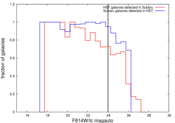
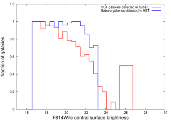
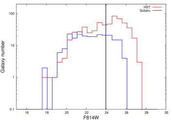
We quantify the difference between the HST and Subaru detections by computing the fraction of galaxies detected in one instrument that is also detected in the other one. We first cross match the catalogs, with a nearest neighbor approach and a maximum distance criterion of , which roughly corresponds to the size of the Subaru PSF. We then measure the fraction of redetected objects, in bins of magnitude, and central SB, and show them for cluster RXJ1347 in Fig. 1. The central SB is estimated as the magnitude in a radius centered on each galaxy, and divided by the aperture area. We see that almost all galaxies detected with Subaru are also detected in HST, and that for magnitudes fainter than 21, Subaru starts to miss galaxies compared to HST, with about 30% of galaxies missed at the Subaru 90% completeness limit. The effect is even clearer when plotting the histograms as a function of SB. We also note a small drop at magnitude , although not significant because corresponding only to one or two galaxies in a bin populated by about 10 galaxies. These two plots show that there is a clear difference due to the SB selection effects between Subaru and HST, but we note that this effect also applies to field galaxies.
3.2 Selecting red sequence galaxies
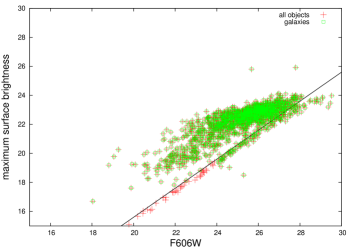
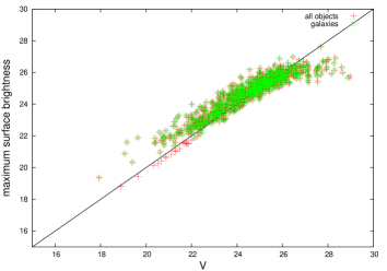
Galaxies are separated from stars in a maximum SB versus magnitude diagram. Point like sources have their maximum SB proportional to their magnitude and can thus be isolated in this diagram up to a certain magnitude. This separation is done independently for the HST and Subaru catalogs, in the filter where the star sequence is best visualized. We discard stars up to F814W=23 for HST and Ic/Ip=21 for Subaru in the I band, and up to F606W=24 and V=22 when the selection is done in the V band. Above these magnitudes it becomes difficult to make a distinction between stars and small galaxies. The magnitude limit is higher for HST because of the smaller PSF which allows for a better separation. We note from the Besançon model (Robin et al., 2003) of the Milky Way star distribution, that the number of stars above i=21 becomes quite low compared to the observed number of galaxies, so the remaining faint stars should not significantly affect the GLF faint end. In addition, these stars should be bluer than cluster galaxies in the studied redshift range, and are very unlikely to be selected in the RS. As an illustration of the star galaxy separation we show in Fig. 2 the diagrams of maximum SB versus magnitude with the star cuts overplotted for cluster RXJ1347.
We then cut the catalog to a circular area centered on the cluster. The radius of this disk is set to the maximum value such that the cluster area is fully included in the HST/ACS field of view (see Table 1). This physical radius is then smaller for low redshift clusters. This choice is made to use all possible data, and because we found that the stacked GLF does not depend on the external radius. See Sect. 4.6 in which we make use of the large field of view of the Subaru/Suprime-Cam images to compute stacked GLFs in various radii.
It has been known for a long time that in a color-magnitude diagram cluster galaxies follow a relation now called the red sequence, which has a very small scatter (Bower et al., 1992). The RS therefore makes the selection of cluster galaxies straightforward when the filter pair samples the 4000 Å break (see e.g. Gladders & Yee, 2000). We plot a F606W-F814W versus F814W diagram for HST and V-Ic versus Ic or V-Ip versus Ip for Subaru. These filters are chosen to bracket the 4000 Å break at the cluster redshifts (), highlighting the red sequence. The RS is fitted by a linear function with a slope fixed to (Durret et al., 2011). We use the same slope for every cluster as it has been shown that the slope does not significantly vary in this redshift range (e.g. De Lucia et al., 2007), which is also what we observe in our color-magnitude diagrams. The zeropoint is first set to the early type galaxy color value in Fukugita et al. (1995) at the cluster redshift, and then re-evaluated in a fit to the RS with a width of in color and using only galaxies brighter than I=23. The final width of the RS is set to , a classical value in the literature (e.g. De Lucia et al., 2007; Martinet et al., 2015). Additionally, Durret et al. (2016) studied the impact of the width of the RS on cluster member selection, and found that this value is a good trade off between including many cluster galaxies and limiting the contamination from field galaxies. As an example we show the HST and Subaru color-magnitude diagrams of RXJ1347 in Fig. 3. The RS is well defined in both data sets. We observe a higher number of galaxies in the HST catalog, especially at the faint end, highlighting the higher sensitivity of space-based telescopes, which can be in part attributed to the SB selection effect described and simulated in De Propris et al. (2013), and shown in Fig. 1 of the present analysis. We note however that the field images are affected in the same way, so that more faint field galaxies are observed in HST than in Subaru.
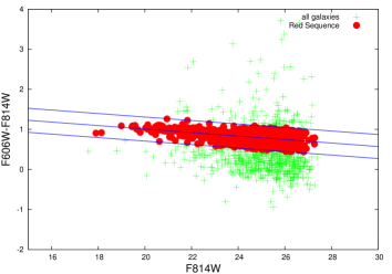
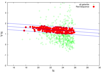
Selecting cluster galaxies through the RS, while requiring only two optical bands, does not allow us to study the blue, often late type, cluster galaxies, which lie below the RS. This can be achieved when galaxy redshifts are available, and has been applied using photometric redshifts in e.g. Martinet et al. (2015). In the present study we will therefore only compute the GLFs for the RS cluster galaxies.
3.3 Computing rest-frame magnitudes
We use LePhare (Arnouts et al., 1999; Ilbert et al., 2006) to compute k-corrections and magnitude shifts to obtain rest-frame magnitudes in the F814W and F606W optical bands for both space and ground based data. Galaxy spectral energy distributions (SEDs) are modeled with emission lines from Polletta et al. (2006, 2007) and extinction laws from Calzetti & Heckman (1999). We then select early type galaxy templates at around each cluster redshift, as those are the most representative of the RS cluster galaxy population. The k-correction and magnitude shifts are set to the mean value over the selected sub-sample of galaxy templates.
We note that RS cluster galaxies have all the same redshifts and similar colors. Therefore, their k-corrections are similar, and we can apply the values computed above to every RS galaxy of each cluster. One consequence is that the histogram of magnitudes for the RS galaxies is not distorted but simply shifted when going from apparent to rest-frame magnitudes. This approach assumes that galaxies with the same redshift and V-I color have the same k-correction, which is found to be reasonable in the Sloan Digital Sky Survey (www.sdss.org) galaxies (Chilingarian et al., 2010). It additionally supposes that the k-corrections are similar across the RS width. Using the online k-correction calculator of Chilingarian et al. (2010); Chilingarian & Zolotukhin (2012) for galaxies below , we estimate the variation of the k-correction across the color scatter in the case of RXJ1347. We find a corresponding k-correction scatter of in the I band and in the V band. We note that these values remain small and do not significantly bias our GLFs which are binned in 0.5 magnitudes. This method is also the best we can do given that we have only two optical bands and therefore cannot perform a proper SED fitting.
3.4 Subtracting field galaxies
Field galaxies are extracted from the COSMOS field the same way as cluster galaxies. Galaxies are separated from stars in a maximum SB versus magnitude diagram up to F814W=23 for HST and Ip=22 for Subaru. For each cluster we apply the same color cut to the field galaxies to select only the galaxies that lie in the cluster RS. We then apply the same k-correction as that computed from the cluster galaxy templates. This approach gives wrong rest-fame magnitudes for the field galaxies because they can be at different redshifts from that of the cluster. However, as the k-correction is assumed to be the same for all selected cluster galaxies, removing field galaxies k-corrected in this way is equivalent to removing field galaxies in apparent magnitude. Normalized field galaxy counts are thus removed from cluster galaxy counts, applying the same k-correction to both samples and binning in slices of 0.5 magnitude.
We recall that the COSMOS area used in the present study is deg2 which is more than ten times larger than any of the cluster area. We investigate possible cosmic variance effects by computing the galaxy number counts as a function of magnitude in 8 independent subareas of our background catalog. Each of these subregions covers one tenth of the full catalog, and is representative of a typical cluster area. We find no significant deviation of the normalized galaxy counts in these subregions from the counts in the full background catalog. This approach underestimates the cosmic variance, that could still affect our results at larger scales, but we cannot probe it with the small area of our background images. For example Muzzin et al. (2013) showed that even the full COSMOS field has a void at , and is therefore subject to cosmic variance.
3.5 Building cluster GLFs
Galaxies are counted in bins of 0.5 magnitude and normalized to one square degree, accounting for masked areas. Error bars are Poisson errors, and correspond to the quadratic sum of the errors on cluster and field counts. The normalization is done after computing the errors to avoid artificially decreasing the error bars.
3.6 Measuring the completeness
Completeness is a crucial point in GLF studies. Overestimating the completeness limit can lead to wrong low faint counts, while underestimating it can mask possible decreases at the faint end. We note that an overestimation is worst because it introduces bins with wrong number counts while the underestimation only artificially degrades the depth of the data. Hence, it is better to adopt a conservative approach when estimating the completeness limit.
The completeness is measured independently for each image, using simulated stars. We apply the same code as in Martinet et al. (2015). We first use our measured PSF to model a set of stars with various magnitudes, and a Gaussian 2D SB profile. We then implement these stars into the original image and try to re-detect them using SExtractor with the same configuration file than that used for the object detection (see Sect. 3.1). Doing so with a thousand stars for each bin of magnitude allows to accurately determine the completeness of the data. The 90% completeness limit is set to the last bin of magnitude at which we still re-detect 90% of the simulated stars, minus 0.5 to take into account the fact that stars are easier to detect than galaxies. Adami et al. (2006) estimated the 90% completeness level for point-like sources and for low surface brightness galaxies in their data, and compared these limits with a deeper catalog. This led them to “assume for galaxies a mean completeness 0.5 mag brighter than the point source 90% completeness levels, whatever the band” (Adami et al., 2007). The positions at which simulated stars are implemented in the images are chosen randomly. Therefore some stars could fall on existing objects biasing the estimate of the completeness limit. This bias should however be small given the small area of the images covered by objects compared to empty regions.
While we measure the completeness for each image, we choose to use the Subaru completeness limits for the deeper HST images, in order to compare GLFs from both telescopes in the same magnitude range. We note that in most cases, this does not significantly affect the fits to the HST GLFs because the Subaru completeness limit is already several bins deeper than the characteristic magnitude , though the errors on the parameters are slightly degraded due to the loss of the faintest bins.
3.7 Fitting cluster GLFs
| (1) |
where is the characteristic absolute magnitude at which the GLF bends from bright to faint galaxies, the faint-end slope of the GLF, and a normalization factor.
We evaluate these three parameters by minimizing the between the Schechter function and the data up to the completeness limit. Parameter error bars correspond to the 1 confidence level, and are computed from the covariance matrix, evaluated at the best parameter values. The final value of the fit is converted into a confidence probability assuming a distribution with three degrees of freedom (,,). This probability of the to be lower than the measured value is equal to the incomplete gamma function estimated at , where is the number of degrees of freedom. For , we find:
| (2) |
There is a known excess of bright galaxies compared to the Schechter function in the case of clusters. While some authors account for this excess, for example by fitting a combination of a Schechter and a Gaussian (e.g. Biviano et al., 1995), we choose to use a simple Schechter function for several reasons. First, using a more complex function with a higher number of parameters decreases the significance of the fit. This is mainly a concern for the high redshift clusters which cover fewer bins of magnitude. Second, the very bright end of the GLF has very high Poisson errors (as high as the signal for the bin containing the Brightest Cluster Galaxy (BCG)), and thus does not significantly affect Schechter parameter estimates. We verify this statement on the stack GLF estimating Schechter parameters taking or not the brightest bins into account, and find a variation of the order of 0.1. Therefore, we can safely neglect this excess when studying the faint end of cluster GLFs.
3.8 Stacking cluster GLFs
Individual cluster GLFs are stacked using Colless stacks (e.g. Colless, 1989; Martinet et al., 2015). The idea of this method is, for each bin of magnitude, to average cluster counts from every cluster that is 90% complete at least up to that bin. Individual counts are first normalized by the cluster richness to avoid being dominated by large clusters. In this study we define the richness as the number of galaxies brighter than the brightest completeness limit of the clusters included in the stack. To get physical galaxy counts, each final bin value is multiplied by the mean richness of all clusters included in that bin.
While this method allows to use the maximum amount of information from the cluster data set, its interpretation requires some care. The main issue is that the number of clusters is different in each magnitude bin. In particular the faintest bins are only populated by clusters with the faintest completeness limit. To avoid the GLF faint end being dominated by one or two very complete clusters, we only take into account the bins that include at least four clusters. This number is chosen based on Martinet et al. (2015) who found that for a given completeness limit, the estimated Schechter parameters tend to remain the same when adding more clusters in the stack. In addition, each bin of magnitude corresponds to a different mean redshift, which can have important consequences given the large redshift range of the studied cluster sample (). Since the absolute magnitude completeness limit is brighter at higher redshifts (assuming that all data have approximately the same depth), the faint bins of the GLF are dominated by the lower redshift clusters. This problem can be attenuated by stacking clusters in redshift bins, though this decreases the significance of the signal.
4 Galaxy luminosity functions: results
We first show the individual (Sect. 4.1) and stacked cluster GLFs (Sect. 4.2). We then study the evolution of the stacked GLFs with redshift (Sect. 4.3) and mass (Sect. 4.4) for the HST and Subaru data. We also investigate binning both in redshift and mass to break the degeneracy between the two parameters (Sect. 4.5). In the case of Subaru, we compute the GLFs as a function of radius as well (Sect. 4.6). Finally, we use simulations to study the effect of SB dimming (Sect. 4.7). As we found that the studied GLFs behave identically in the F606W and F814W filters, we only show them in the latter filter, to improve the paper readability.
4.1 Individual cluster GLFs
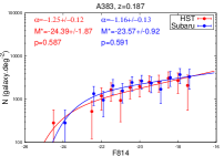
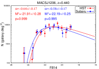
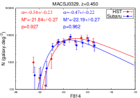
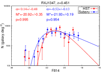
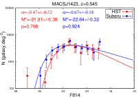
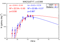
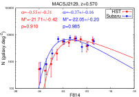
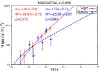
Figure 4 shows the individual cluster GLFs in the F814W band. We note a good overall agreement between the Subaru (in blue) and HST GLFs (in red). As a general trend we find that the faint end seems to be flatter for the lower redshifts. However, the Schechter parameters from the fits have large error bars, and a large dispersion across clusters. This highlights the need for stacking to infer precise results on the faint end slope and the characteristic magnitude . The Schechter parameters from the fits to individual clusters are displayed in Appendix A.
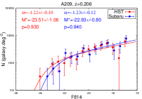
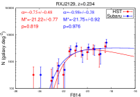
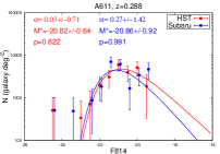
|
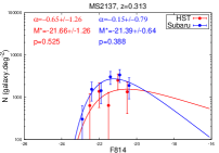
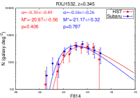
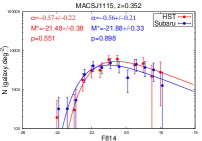
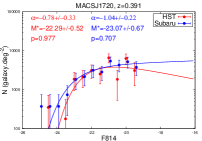
|
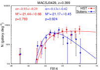
|
|
4.2 Stacked cluster GLFs
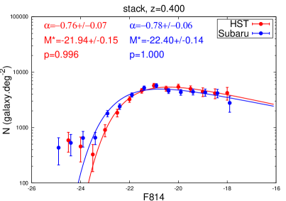
The stacked GLFs for all 16 clusters are presented in Fig. 5. We find a very good agreement between the HST and Subaru GLFs, with equal faint end slopes given the error bars and only a slightly higher for Subaru. We find for HST and for Subaru, the mean redshift of clusters being , and the fit extending to more than . Even at this depth we cannot investigate the possible upturn of the GLF which is seen in the very faint population of nearby clusters (e.g. Popesso et al., 2006). We also note an expected excess at the very bright end of the GLF, as discussed in Sect. 3.7. GLFs included in the stack are computed within a circle centered on the cluster center with the largest possible radius given the HST field of view. Therefore each cluster covers a different area but we show in Sect. 4.6 that the stacked GLFs do not depend on the radius in which they are computed in the range [0.5:2.5] Mpc, and with the present completeness limits.
Comparable results are found in the F606W filter, but since the data are not as deep as in the F814W filter we do not show them here.
4.3 Evolution with redshift
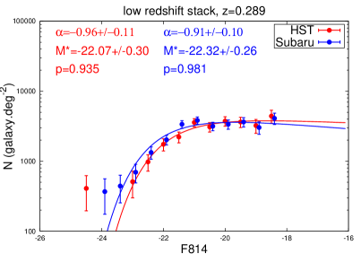
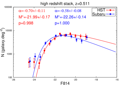
As the faint end of the Colless stack is dominated by the most complete, hence the lowest redshift clusters, we separate our sample into two redshift bins. This allows us to better quantify the evolution of the faint end with redshift. The low redshift sample is composed of 8 clusters with , and the high redshift sample of 8 clusters with . Results are displayed in Fig. 6.
The redshift segregation highlights some possible differences between the HST and Subaru GLFs, but we still note a decrease of the faint end when the redshift increases. In the lower redshift case, both GLFs agree, and we find and for HST and Subaru data respectively. We note that the faint end now agrees with a flat faint end value (), for a mean redshift of . In the high redshift case, the faint ends computed with HST and Subaru data differ at a 0.9 level, with and , providing a hint of a SB selection effect, but not at a significant level. The change in between the low and high redshift cases is 1.7 and 2.6 for HST and Subaru respectively. While faint object selections are different for HST and Subaru, leading to higher faint galaxy counts in the former instrument at high redshift, we still find a decreasing faint end with increasing redshift. In Sect. 4.7 we use simulations to check whether the observed evolution with redshift can be attributed to SB dimming.
4.4 Dependence on mass
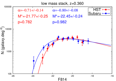
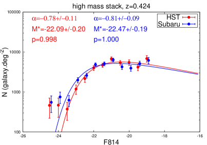
Using total masses computed from joint weak and strong lensing by Umetsu et al. (2016), and given in Table 1, we can separate clusters into low mass () and high mass () samples. Two clusters in the present study are not part of the Umetsu et al. (2016) sample. However they can be safely classified as low mass for MACSJ1423 and high mass for MACSJ2129, according to the strong lensing analysis of Zitrin et al. (2011). In addition, Martinet et al. (2016) derived a weak lensing mass of for MACSJ1423, in agreement with its strong lensing classification. Given that we only discriminate clusters according to a mass threshold, accurate masses are not required, providing that the threshold is excluded by the mass error bars, which is the case for most of our clusters. There are 6 low mass clusters and 10 high mass. We could have chosen a mass threshold such that we have 8 clusters in every stack, but this would result in having clusters of masses in the low mass sample, while a cluster of is already a very massive cluster. The low-mass sample has a median mass of , and the high-mass of .
Results are shown in Fig. 7. The faint ends from HST and Subaru agree within the error bars while the characteristic magnitudes are brighter for Subaru, especially when considering the low mass sample. We find no significant evolution of the GLF faint end slope with mass, for both sets of data, with and for HST low and high mass clusters, and and for Subaru low and high mass clusters respectively. However, we note that there might be a degeneracy with redshift, as the low mass sample has a mean redshift and the high mass . If high mass clusters were showing flatter faint ends, this could compensate for redshift evolution.
4.5 Breaking the degeneracy between redshift and mass
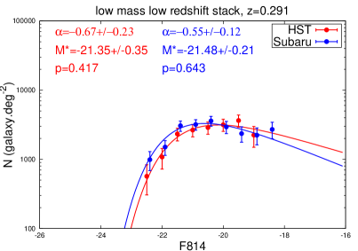
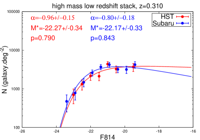
In this section we try to break the degeneracy between redshift and mass by making four samples: low mass/low z (4 clusters), low mass/high z (2 clusters), high mass/low z (5 clusters), and high mass/high z (5 clusters). Given the few clusters in the low mass/high z, and the large error bars due to brighter completeness limit in the high mass/high z sample, we can only investigate the low mass/low z and high mass/low z samples. The median masses for these two samples are and for the low and high mass respectively.
Results are displayed in Fig. 8. The HST and Subaru GLFs agree given the large error bars. We find faint end slopes and for HST low and high mass low z samples, and and for Subaru low and high mass low z samples. This tends to show that once the degeneracy with redshift is broken, the high mass clusters show a flatter faint end than the low mass. However, this hint is detected at only 1.1 and 1.2, so it would require a larger sample to be verified.
 |
 |
4.6 Dependence on outer radius
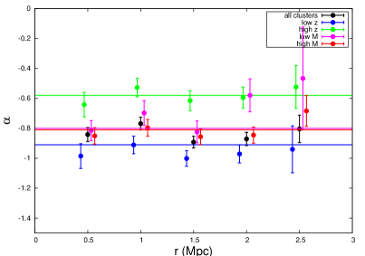
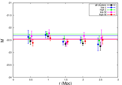
We also take advantage of the large field of view of the Subaru data to investigate how the GLFs may vary with the radius in which they are calculated. For this, we first compute individual cluster GLFs in increasing disks with the following radii: 0.5 Mpc, 1 Mpc, 1.5 Mpc, 2 Mpc, and 2.5 Mpc, before stacking them together. In this way, we cover different areas from the cluster core to the virial radius.
We show in Fig. 9 the parameters and as a function of radius for the whole sample (black dots), for the low (blue) and high (green) redshift samples, and for the low (magenta) and high (red) mass samples, for Subaru data in the F814W filter. We find no significant variation of the faint end slope with radius, with values of consistent with those found in the previous sections (horizontal lines). The characteristic magnitudes slightly vary for radii greater than 1 Mpc, but only at a 1 level. These results suggest that the GLFs are dominated by the cluster core, and they don’t change when the radius of the considered region increases, at least with the present completeness limit. The only variation seen is in the low mass sample at radii greater than 2 Mpc. These clusters being less rich, they start to be dominated by field galaxies when extending to high radii, leading to less negative faint end slopes representative of field GLFs (e.g. Zucca et al., 2006; Martinet et al., 2015). We note however that it does not affect the other results of the paper, as clusters are studied in radii lower than 1 Mpc in the rest of this study due to the limited size of the HST images.
4.7 Simulating surface brightness dimming
In Sect. 4.3 we found that the GLF faint end shows a mild dependence on redshift in our sample. We now want to assess if this redshift evolution can be attributed to the dimming of galaxy SB with redshift. Indeed, SB has a dependence on redshift: . A factor is due to the dimming of the flux when the same galaxy is observed at higher redshift and the other factor accounts for the change in the angular area. Although we expect to miss some of the higher redshift galaxies due to the SB dimming, we note that the dimming is the same for both datasets, and is therefore a separate problem from that of the SB selection effect between datasets.
If we note the angular radius and the physical radius of a galaxy, those are linked through the angular distance :
| (3) |
where is the comoving distance and the redshift of the galaxy. Assuming that the physical radius of a galaxy is the same whichever the redshift111Ignoring size evolution is a conservative estimate as galaxies are smaller at high redshift (van Dokkum & van der Marel, 2007) and this would make their SB brighter., one can write the fractional change in angular radius from a redshift to .
| (4) |
To calculate the change in total flux of the galaxy we not only have to consider the change in luminosity distance and the k-correction, but also the change in luminosity that comes from the luminosity evolution of each galaxy. We adopt the luminosity evolution inferred from the fundamental plane evolution, assuming that this evolution is purely luminosity dependent (i.e. that there is no evolution in the physical size). We use equation (10) of van Dokkum & van der Marel (2007) (recalled in eq. 5 below) who measured the fundamental plane evolution in the redshift range which includes the redshift interval of the present study.
| (5) |
For passive evolution, the mass of the galaxy remains constant and eq. 5 allows to calculate of the change in luminosity in the B band. We furthermore add a k-correction to this relation, noted , to shift it to the F814 filter, and calculate the change in luminosity:
| (6) |
The k-correction is computed using LePhare with the same templates as in the rest of the paper, but adding the B filter to the analysis.
We can now compute the flux dimming which depends on the luminosity distance and on the luminosity ratio of eq. 6. The conversion from bolometric flux to the given filters is taken into account in the k-correction in the luminosity term and therefore does not appear in this equation.
| (7) |
We can use the set of equations given above to compute the SB dimming of cluster galaxies when we shift them from low redshift to high redshift. In particular we want to simulate images of the low redshift cluster sample as they would appear at higher redshift. We shift every low redshift cluster by the difference in mean redshift of the high and low redshift samples. Comparing the stacked GLFs of the low and high redshift simulated images to those of the observed data allows to check whether SB dimming can explain the observed redshift evolution or not.
Simulations are made with the GalSim software (Rowe et al., 2015),
using galaxies measured on the observed images. The PSF is measured
on each image with PSFEx, and Sersic profiles convolved with this
PSF are fitted to galaxies using SExtractor. The parameters from this
fit are then used in GalSim to simulate galaxies as single Sersic
profiles with half-light radius, Sersic index, flux, and position
from the original image. In the case of the high-redshift simulations, we apply the evolution given in eqs. 4 & 7 to the radii and fluxes measured on the low-redshift galaxies before using these quantities in the simulations. These profiles are then convolved with an
analytic Moffat PSF with (following prescriptions from Trujillo et al., 2001) and the measured
FWHM, before being inserted into the images. The pixel scale is the same as
in the data (0.03” for HST and 0.2” for Subaru) and we add
Gaussian random noise with the sky rms value measured in the image
by SExtractor. We keep the same noise seed for the fiducial
simulations (with the low redshift clusters) and the high redshift ones.
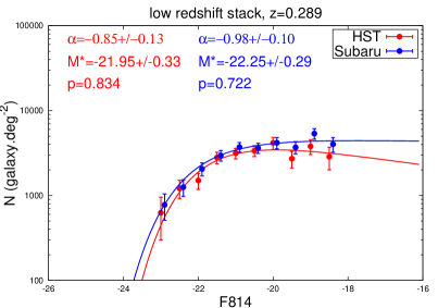
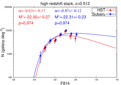
Figure 10 shows the stacked GLFs for the low redshift simulated sample and the same clusters evolved to the mean redshift of the high redshift sample. These GLFs are to be compared with the observed redshift evolution (Fig. 6). First we see that the simulated low-redshift GLF is not identical to the observed one due to the fact that the simulations are simplistic compared to real data. However the simulated and observed GLFs agree within the error bars with a difference of 0.6 for HST and 0.5 for Subaru, validating our simulation pipeline.
Looking at the simulated high-redshift sample we find that the slope of the GLF has slightly decreased compared to the low redshift simulation. We find that the slope for the simulated clusters varies by 1.0 and 0.7 from low to high redshift respectively for HST and Subaru. We interpret this change as coming from SB selection. These values are to be compared with the 1.7 and 2.6 variation in the case of the observations. We therefore conclude that SB dimming is not sufficient to explain alone the observed redshift evolution of the faint end of the GLF. The small observed evolution may also be due to our relatively small redshift baseline, and a larger range of redshifts would be valuable to secure our findings. We also investigate how robust these results are to the knowledge of the fundamental plane by computing the variation of the faint end slope when applying the error bars of eq. 5. The slope of the evolved stacked GLF varies of and , in the case of HST and Subaru respectively, when considering these error bars. We note that is not significantly affected by SB dimming, which we can expect as the bright galaxies should be visible regardless of the SB dimming.
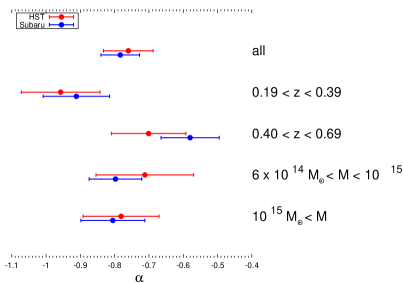
5 Discussion
We compute the stacked GLFs for 16 CLASH clusters based on independent
HST and Subaru analyses in order to study the faint end and the
characteristic magnitude of cluster RS GLFs in the redshift range
, and their evolution with redshift and mass. A
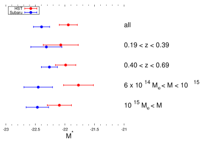
summary of the main results can be found in Fig. 11,
where we plot and values for the whole sample and for the
subsamples in the different redshift and mass ranges. The use of both
space and ground based data enables us to discuss selection effects, while simulations permit to investigate the effect of SB dimming with redshift (cf. Fig. 10). In addition, the Subaru large field of view allows
to study the dependence on radius, and results on this point are
displayed in Fig. 9 in
Sect. 4.6. Based on these figures, the main results
of our analysis are the following:
1. We find no dependence of or on radius in the range
0.5 to 2.5 Mpc, except for low mass clusters at radius greater than 2 Mpc. This probably means that cluster GLFs are dominated by
the cluster core in the probed magnitude range. We can therefore
be certain that the smaller size of the HST field of view is not
responsible for the different faint end behaviors observed in the
literature.
2. We find no evolution of either with redshift or mass,
suggesting that the bright population is similar in the studied
redshift and mass ranges. We recall that the lowest mass of our
clusters is , so they are all quite massive,
explaining that they have similar abundances of bright
galaxies. However, we find that the value derived from HST is
magnitude fainter than that from Subaru. A possible
explanation would be a leakage of stars into the GLF bright end, as
the star-galaxy separation is not as good in the Subaru data due to
the larger PSF. However, we could not find evidence for this by visual
inspection, as it is difficult to discriminate between
stars and galaxies with circular shapes at these magnitudes. Another explanation might reside in the low statistics of the background subtraction at the bright end, which could introduce small differences between the bright ends of the two data sets.
3. Using the whole sample (), we find a decreasing faint end for both datasets with consistent values between HST () and Subaru (). Separating between a low redshift () and high redshift () samples, we find an evolution of the faint end slope of 1.7 with HST and 2.6 with Subaru. There is thus a mild decrease of the faint end slope (less negative ) with increasing redshift over the range (). This evolution is in good agreement with recent papers in the literature: in particular Zenteno et al. (2016) found a decrease of the RS faint end at for a wider range of redshifts (), but with of their clusters being in the same redshift range as ours.
De Propris et al. (2013) claimed that the evolution in the faint end slope has a significant contribution from surface brightness selection effects. They used HST data of differing depths on a single cluster (MS 1358.4+6254) to show that surface brightness selection effects become important above the formal magnitude limit of their data and that they affect the red sequence GLF at magnitudes z24.5 for 2.7 ksec HST exposures (see their Fig. 18). Given that the faint red sequence for their cluster has , this implies that the SB selection effects in their sample become important at . On the other hand, our CLASH data are significantly deeper than theirs (4.1 ksec) and we limit our GLFs at . Therefore, the real SB selection effects noticed in De Propris et al. (2013) should not be playing a role in our space-based results.
In addition, De Propris et al. (2013) claim that previous estimates of
the evolution in the red sequence GLF
(e.g. De Lucia et al., 2007; Rudnick et al., 2009) were also due to SB effects.
Both of those works were based on the same ground-based data with a
formal magnitude limit of I or 24.5 (for the low and high redshift
clusters respectively) and the evolution in the GLF was seen over
the faintest 2 magnitudes. We cannot directly address the role of
SB effects in the EDisCS results without detailed simulations on
those data (see below for such simulations for our clusters) but the
similarity between our HST and Subaru GLFs imply that the EDisCS
evolution in the GLF is not dominated by SB effects.
4. We artificially evolved the low redshift clusters to high
redshifts, through simulations taking into account the fundamental
plane evolution and SB dimming. Computing the GLFs
from these simulations we find no evolution of with redshift
and no significant evolution of , namely and
for HST and Subaru respectively. Surface brightness dimming
therefore cannot explain the redshift evolution of the GLF
observed in the data.
5. We see no significant trend of the faint end with mass, but
maybe because all of our clusters are quite massive. We note that this
result agrees with the weak dependence on mass found in
e.g. De Lucia et al. (2007); Gilbank et al. (2008); Rudnick et al. (2009). Cerulo et al. (2016)
found hints that more massive clusters could have flatter GLFs for
high redshift clusters (), but it seems not to be the case
at lower redshifts, at least in the mass range probed here.
Though SB selection effects and SB dimming affect the high redshift cluster GLFs, they are not sufficient to explain alone the deficit of RS galaxies up to , which therefore requires some physical process such as quenching of star formation. As there is also no dependence of the GLFs on the image field of view, the number of possible explanations to the differences found in the literature becomes smaller. One last point worth investigating is the selection of clusters, as all studies, including the present one, select small sets of clusters (typically a few to a few tens of clusters), and are based on different criteria. The only way to uncover this problem is to build a very large sample of galaxy clusters, such as the one that will be available in upcoming large optical surveys.
Acknowledgements.
We thank the referee for useful comments which improved the quality and readability of the paper. We are very grateful to the CLASH team for making their data publicly available. For the same reason we also thank the 3D-HST team for the COSMOS reduced images. Finally we thank the GalSim team and Emmanuel Bertin for their respective public software and additionally Emmanuel for useful discussions. Florence Durret acknowledges long-term support from CNES. Gregory Rudnick acknowledges support of NSF funding from proposals 1517815 and 1211358.References
- Adami et al. (2007) Adami, C., Durret, F., Mazure, A., et al. 2007, A&A, 462, 411
- Adami et al. (2006) Adami, C., Picat, J. P., Savine, C., et al. 2006, A&A, 451, 1159
- Andreon (2006) Andreon, S. 2006, MNRAS, 369, 969
- Arnouts et al. (1999) Arnouts, S., Cristiani, S., Moscardini, L., et al. 1999, MNRAS, 310, 540
- Bertin (2011) Bertin, E. 2011, in Astronomical Society of the Pacific Conference Series, Vol. 442, Astronomical Data Analysis Software and Systems XX, ed. I. N. Evans, A. Accomazzi, D. J. Mink, & A. H. Rots, 435
- Bertin & Arnouts (1996) Bertin, E. & Arnouts, S. 1996, A&AS, 117, 393
- Biviano et al. (1995) Biviano, A., Durret, F., Gerbal, D., et al. 1995, A&A, 297, 610
- Bower et al. (1992) Bower, R. G., Lucey, J. R., & Ellis, R. S. 1992, MNRAS, 254, 601
- Brammer et al. (2012) Brammer, G. B., van Dokkum, P. G., Franx, M., et al. 2012, ApJS, 200, 13
- Calzetti & Heckman (1999) Calzetti, D. & Heckman, T. M. 1999, ApJ, 519, 27
- Capak et al. (2007) Capak, P., Aussel, H., Ajiki, M., et al. 2007, ApJS, 172, 99
- Cerulo et al. (2016) Cerulo, P., Couch, W. J., Lidman, C., et al. 2016, MNRAS, 457, 2209
- Chilingarian et al. (2010) Chilingarian, I. V., Melchior, A.-L., & Zolotukhin, I. Y. 2010, MNRAS, 405, 1409
- Chilingarian & Zolotukhin (2012) Chilingarian, I. V. & Zolotukhin, I. Y. 2012, MNRAS, 419, 1727
- Colless (1989) Colless, M. 1989, MNRAS, 237, 799
- De Lucia et al. (2004) De Lucia, G., Poggianti, B. M., Aragón-Salamanca, A., et al. 2004, ApJ, 610, L77
- De Lucia et al. (2007) De Lucia, G., Poggianti, B. M., Aragón-Salamanca, A., et al. 2007, MNRAS, 374, 809
- De Propris et al. (2013) De Propris, R., Phillipps, S., & Bremer, M. N. 2013, MNRAS, 434, 3469
- De Propris et al. (2007) De Propris, R., Stanford, S. A., Eisenhardt, P. R., Holden, B. P., & Rosati, P. 2007, AJ, 133, 2209
- Durret et al. (2011) Durret, F., Laganá, T. F., & Haider, M. 2011, A&A, 529, A38
- Durret et al. (2016) Durret, F., Márquez, I., Acebrón, A., et al. 2016, A&A, 588, A69
- Ford et al. (2003) Ford, H. C., Clampin, M., Hartig, G. F., et al. 2003, in Proc. SPIE, Vol. 4854, Future EUV/UV and Visible Space Astrophysics Missions and Instrumentation., ed. J. C. Blades & O. H. W. Siegmund, 81–94
- Fukugita et al. (1995) Fukugita, M., Shimasaku, K., & Ichikawa, T. 1995, PASP, 107, 945
- Gaidos (1997) Gaidos, E. J. 1997, AJ, 113, 117
- Gilbank et al. (2008) Gilbank, D. G., Yee, H. K. C., Ellingson, E., et al. 2008, ApJ, 673, 742
- Gladders & Yee (2000) Gladders, M. D. & Yee, H. K. C. 2000, AJ, 120, 2148
- Ilbert et al. (2006) Ilbert, O., Arnouts, S., McCracken, H. J., et al. 2006, A&A, 457, 841
- Martinet et al. (2016) Martinet, N., Clowe, D., Durret, F., et al. 2016, A&A, 590, A69
- Martinet et al. (2015) Martinet, N., Durret, F., Guennou, L., et al. 2015, A&A, 575, A116
- Miyazaki et al. (2002) Miyazaki, S., Komiyama, Y., Sekiguchi, M., et al. 2002, PASJ, 54, 833
- Muzzin et al. (2013) Muzzin, A., Marchesini, D., Stefanon, M., et al. 2013, ApJ, 777, 18
- Paolillo et al. (2001) Paolillo, M., Andreon, S., Longo, G., et al. 2001, A&A, 367, 59
- Polletta et al. (2007) Polletta, M., Tajer, M., Maraschi, L., et al. 2007, ApJ, 663, 81
- Polletta et al. (2006) Polletta, M. d. C., Wilkes, B. J., Siana, B., et al. 2006, ApJ, 642, 673
- Popesso et al. (2006) Popesso, P., Biviano, A., Böhringer, H., & Romaniello, M. 2006, A&A, 445, 29
- Postman et al. (2012) Postman, M., Coe, D., Benítez, N., et al. 2012, ApJS, 199, 25
- Robin et al. (2003) Robin, A. C., Reylé, C., Derrière, S., & Picaud, S. 2003, A&A, 409, 523
- Rowe et al. (2015) Rowe, B. T. P., Jarvis, M., Mandelbaum, R., et al. 2015, Astronomy and Computing, 10, 121
- Rudnick et al. (2009) Rudnick, G., von der Linden, A., Pelló, R., et al. 2009, ApJ, 700, 1559
- Schechter (1976) Schechter, P. 1976, ApJ, 203, 297
- Schlegel et al. (1998) Schlegel, D. J., Finkbeiner, D. P., & Davis, M. 1998, ApJ, 500, 525
- Skelton et al. (2014) Skelton, R. E., Whitaker, K. E., Momcheva, I. G., et al. 2014, ApJS, 214, 24
- Smail et al. (1998) Smail, I., Edge, A. C., Ellis, R. S., & Blandford, R. D. 1998, MNRAS, 293, 124
- Stott et al. (2007) Stott, J. P., Smail, I., Edge, A. C., et al. 2007, ApJ, 661, 95
- Tanaka et al. (2005) Tanaka, M., Kodama, T., Arimoto, N., et al. 2005, MNRAS, 362, 268
- Taniguchi et al. (2007) Taniguchi, Y., Scoville, N., Murayama, T., et al. 2007, ApJS, 172, 9
- Trujillo et al. (2001) Trujillo, I., Aguerri, J. A. L., Cepa, J., & Gutiérrez, C. M. 2001, MNRAS, 328, 977
- Umetsu et al. (2016) Umetsu, K., Zitrin, A., Gruen, D., et al. 2016, ApJ, 821, 116
- van Dokkum & van der Marel (2007) van Dokkum, P. G. & van der Marel, R. P. 2007, ApJ, 655, 30
- Vulcani et al. (2011) Vulcani, B., Poggianti, B. M., Aragón-Salamanca, A., et al. 2011, MNRAS, 412, 246
- Zenteno et al. (2016) Zenteno, A., Mohr, J. J., Desai, S., et al. 2016, MNRAS, 462, 830
- Zitrin et al. (2011) Zitrin, A., Broadhurst, T., Barkana, R., Rephaeli, Y., & Benítez, N. 2011, MNRAS, 410, 1939
- Zucca et al. (2006) Zucca, E., Ilbert, O., Bardelli, S., et al. 2006, A&A, 455, 879
Appendix A Individual cluster GLFs: Schechter parameters
The Schechter parameters for the individual cluster GLFs are given in Table A.1.
| F606W | F814W | ||||||||||
|---|---|---|---|---|---|---|---|---|---|---|---|
| M* | * () | comp | M* | * () | comp | ||||||
| A383 | 0.19 | ||||||||||
| HST | -1.12 0.17 | -21.5 0.7 | 2176 1306 | -16.2 | 0.787 | -1.25 0.12 | -24.4 1.9 | 706 674 | -17.4 | 0.587 | |
| Subaru | -0.90 0.19 | -21.3 0.6 | 4073 1886 | -16.2 | 0.971 | -1.16 0.13 | -23.6 0.9 | 1474 899 | -17.4 | 0.591 | |
| A209 | 0.21 | ||||||||||
| HST | -1.22 0.12 | -22.7 1.1 | 1672 1219 | -16.0 | 0.956 | -1.22 0.10 | -23.5 1.1 | 1461 933 | -16.8 | 0.930 | |
| Subaru | -1.29 0.09 | -23.4 1.1 | 1126 775 | -16.0 | 0.769 | -1.23 0.12 | -22.9 0.8 | 1738 1085 | -16.7 | 0.940 | |
| RXJ2129 | 0.23 | ||||||||||
| HST | -0.70 0.50 | -20.7 0.8 | 5706 3897 | -17.9 | 0.751 | -0.75 0.48 | -21.2 0.8 | 5504 3880 | -18.1 | 0.819 | |
| Subaru | -1.05 0.35 | -21.3 0.9 | 3651 3240 | -17.9 | 0.969 | -0.98 0.38 | -21.8 0.9 | 3894 3406 | -18.1 | 0.976 | |
| A611 | 0.29 | ||||||||||
| HST | -0.06 1.05 | -20.4 0.9 | 13874 4078 | -19.0 | 0.640 | 0.03 0.71 | -20.8 0.6 | 14141 3173 | -19.1 | 0.622 | |
| Subaru | 0.63 1.88 | -20.0 1.0 | 12367 8026 | -19.0 | 0.834 | 0.27 1.42 | -20.9 0.9 | 12888 2328 | -19.1 | 0.991 | |
| MS2137 | 0.31 | ||||||||||
| HST | -1.81 2.56 | -22.0 4.2 | 1147 8555 | -20.3 | 0.182 | -0.65 1.26 | -21.7 1.3 | 3450 3608 | -20.3 | 0.525 | |
| Subaru | -1.38 1.32 | -21.8 2.0 | 3109 8242 | -20.3 | 0.064 | -0.15 0.79 | -21.4 0.6 | 7942 2276 | -20.3 | 0.388 | |
| RXJ1532 | 0.34 | ||||||||||
| HST | -0.33 0.66 | -20.5 0.7 | 10413 4063 | -17.7 | 0.502 | -0.30 0.49 | -21.0 0.6 | 10409 3365 | -18.1 | 0.406 | |
| Subaru | -0.37 0.42 | -20.6 0.7 | 10024 4002 | -17.7 | 0.960 | -0.16 0.26 | -21.2 0.3 | 12004 2017 | -18.1 | 0.787 | |
| MACSJ1115 | 0.35 | ||||||||||
| HST | -0.41 0.36 | -21.1 0.4 | 11353 3508 | -18.1 | 0.984 | -0.57 0.22 | -21.5 0.4 | 12807 3714 | -17.6 | 0.551 | |
| Subaru | -0.59 0.26 | -21.1 0.3 | 10480 3211 | -18.1 | 0.799 | -0.56 0.21 | -21.9 0.3 | 10336 2977 | -17.6 | 0.898 | |
| MACSJ1720 | 0.39 | ||||||||||
| HST | -0.80 0.35 | -22.0 0.6 | 7384 4198 | -18.6 | 0.916 | -0.78 0.33 | -22.3 0.5 | 7173 3573 | -19.4 | 0.977 | |
| Subaru | -1.23 0.30 | -22.4 1.0 | 3225 3216 | -18.6 | 0.624 | -1.04 0.22 | -23.1 0.7 | 4552 2796 | -19.4 | 0.707 | |
| MACSJ0429 | 0.40 | ||||||||||
| HST | - | - | - | -19.2 | - | -0.93 0.29 | -21.4 0.7 | 6864 4177 | -18.0 | 0.783 | |
| Subaru | 0.40 0.80 | -20.1 0.5 | 12688 2863 | -19.2 | 0.860 | -0.13 0.42 | -21.2 0.5 | 11973 2930 | -18.0 | 0.924 | |
| MACSJ1206 | 0.44 | ||||||||||
| HST | -0.64 0.17 | -21.4 0.3 | 19228 4481 | -18.4 | 0.999 | -0.64 0.17 | -21.9 0.3 | 18184 4269 | -18.8 | 0.999 | |
| Subaru | -0.70 0.15 | -21.9 0.3 | 15520 3896 | -18.4 | 0.906 | -0.58 0.17 | -22.2 0.3 | 18173 4074 | -18.8 | 0.995 | |
| MACSJ0329 | 0.45 | ||||||||||
| HST | -0.66 0.29 | -21.5 0.3 | 17008 5178 | -19.1 | 0.990 | -0.54 0.23 | -21.8 0.3 | 18812 4508 | -19.4 | 0.927 | |
| Subaru | -0.55 0.29 | -21.6 0.4 | 16801 4957 | -19.1 | 0.942 | -0.47 0.22 | -22.2 0.3 | 17184 3932 | -19.4 | 0.962 | |
| RXJ1347 | 0.45 | ||||||||||
| HST | 0.19 0.62 | -20.4 0.4 | 18248 2539 | -18.6 | 0.996 | 0.14 0.48 | -20.9 0.4 | 17931 2431 | -18.4 | 0.995 | |
| Subaru | -0.01 0.45 | -20.6 0.4 | 18032 3032 | -18.6 | 0.971 | -0.52 0.13 | -21.9 0.2 | 13436 2238 | -18.4 | 0.954 | |
| MACSJ1423 | 0.55 | ||||||||||
| HST | -0.59 0.42 | -21.7 0.6 | 9613 4589 | -19.5 | 0.564 | -0.47 0.32 | -21.9 0.4 | 10500 3341 | -19.0 | 0.766 | |
| Subaru | -0.59 0.34 | -21.6 0.5 | 10491 3959 | -19.5 | 0.638 | -0.67 0.18 | -22.6 0.3 | 9187 2760 | -19.0 | 0.924 | |
| MACSJ0717 | 0.55 | ||||||||||
| HST | -1.11 0.51 | -22.5 0.7 | 11048 9466 | -21.0 | 0.783 | -0.84 0.44 | -22.5 0.6 | 15871 9138 | -20.5 | 0.836 | |
| Subaru | -0.73 0.49 | -21.8 0.4 | 18568 7307 | -21.0 | 0.997 | -0.62 0.28 | -22.7 0.4 | 16367 4885 | -20.5 | 0.987 | |
| MACSJ2129 | 0.57 | ||||||||||
| HST | -0.43 1.13 | -21.2 1.0 | 17761 10170 | -20.2 | 0.618 | -0.55 0.31 | -21.7 0.4 | 15777 5236 | -19.1 | 0.910 | |
| Subaru | -0.52 0.45 | -21.4 0.4 | 19823 5473 | -20.2 | 0.337 | -0.37 0.16 | -22.0 0.2 | 18698 2794 | -19.1 | 0.985 | |
| MACSJ0744 | 0.69 | ||||||||||
| HST | - | - | - | -21.5 | - | -2.00 0.41 | -24.9 2.7 | 371 1416 | -21.3 | 0.013 | |
| Subaru | - | - | - | -21.5 | - | -1.59 0.31 | -25.6 2.9 | 361 960 | -21.3 | 0.994 |