Models and algorithms for the next generation of glass transition studies
Abstract
Successful computer studies of glass-forming materials need to overcome both the natural tendency to structural ordering and the dramatic increase of relaxation times at low temperatures. We present a comprehensive analysis of eleven glass-forming models to demonstrate that both challenges can be efficiently tackled using carefully designed models of size polydisperse supercooled liquids together with an efficient Monte Carlo algorithm where translational particle displacements are complemented by swaps of particle pairs. We study a broad range of size polydispersities, using both discrete and continuous mixtures, and we systematically investigate the role of particle softness, attractivity and non-additivity of the interactions. Each system is characterized by its robustness against structural ordering and by the efficiency of the swap Monte Carlo algorithm. We show that the combined optimisation of the potential’s softness, polydispersity and non-additivity leads to novel computer models with excellent glass-forming ability. For such models, we achieve over ten orders of magnitude gain in the equilibration timescale using the swap Monte Carlo algorithm, thus paving the way to computational studies of static and thermodynamic properties under experimental conditions. In addition, we provide microscopic insights into the performance of the swap algorithm which should help optimizing models and algorithms even further.
I Introduction
Computer simulations play an increasingly important role in elucidating the nature of the glass transition because they allow particle-level resolution of any relevant static or dynamic observable Berthier and Biroli (2011). While a similar spatial resolution can now be achieved in experiments performed with colloids Hunter and Weeks (2012), less direct microscopic information is available from experimental studies of molecular liquids Ediger (2000). Regarding timescales, however, colloidal experiments and computer simulations cover at best the first 4-5 decades of the dynamic slowing down of systems approaching a glass transition Brambilla et al. (2009), whereas 12-13 orders of magnitude of glassy slowdown can be analyzed in molecular liquids Blochowicz et al. (2005). Therefore, the exquisite level of detail gained from simulations in the description of the onset of slow dynamics concerns a dynamical regime which is separated from experiments on molecular glasses by about eight orders of magnitude. The dichotomy between accessible length-scales and timescales is a major challenge for glass transition studies Richert and Angell (1998); Debenedetti and Stillinger (2001); Berthier and Biroli (2011).
There are several promising experimental advances which could improve either the dynamic range of colloidal experiments Hell (2007) or the spatial resolution in molecular supercooled liquids Ashtekar et al. (2010). In addition, new protocols to prepare molecular glasses corresponding to even larger relaxation times are being developed Swallen et al. (2007). On the simulation front, the situation appears challenging, as the increase in the time window accessible to computer simulations has been rather slow, amounting to a gain of about 3 orders of magnitude over the last 30 years Barrat et al. (1990); Kob and Andersen (1995); Brambilla et al. (2009), and this is mostly due to improvements in computer hardware. A rough extrapolation of this trend would pessimistically suggest that it could take another 100 years for simulations to close the gap with experimentally relevant thermodynamic conditions. The recent advent of graphic processing units and accelerators in the high-performance computing arena suggests that progress could be made at a faster pace if novel technologies become available. Exploiting them in the context of molecular simulations Anderson et al. (2008); Colberg and Höfling (2011); Bailey et al. (2015); Anderson et al. (2013); Meyer (2013) requires nonetheless a substantial investment in code development and low-level optimization.
The above summary suggests that it is desirable to develop alternative strategies, which do not simply rely on the brute force increase of computing power. A possible path is to take advantage of the flexibility offered by simulations and implement algorithms that simulate equilibrium material properties more efficiently Newman and Barkema (1999). Several such strategies have already been explored. A first line of research concerns the development of collective particle displacements to improve sampling efficiency Dress and Krauth (1995); Santen and Krauth (2000); Bernard and Krauth (2011). This approach follows the method employed to study phase transitions in spin systems Swendsen and Wang (1987); Binder (1992). For instance, the event-chain Monte Carlo algorithm has proved useful in the study of two-dimensional melting Bernard and Krauth (2011), but its gain in efficiency for the three-dimensional dense fluids considered here is at most a factor of 40 Isobe and Krauth (2015), which remains insufficient to close the gap with experiments. A crucial aspect for the efficiency of this approach is the choice of the correct type of collective move, which still requires some a priori knowledge of the relaxation path used by the system Vink (2014). This, however, is precisely one of the informations that remains to be understood in fragile glass-forming materials.
A different simulation strategy is the replica-exchange technique, where simulations of the same system are conducted in parallel over a range of state points, and infrequent exchanges between neighboring state points are performed Hukushima and Nemoto (1996); Hukushima et al. (1998); Yamamoto and Kob (2000); Odriozola and Berthier (2011). The idea is that navigating through different state points would facilitate the crossing of large barriers in a complex free energy landscape, and indeed the technique was first developed to study spin glasses Hukushima and Nemoto (1996). In dense fluids the reported speedup is again of about two orders of magnitude Yamamoto and Kob (2000); Odriozola and Berthier (2011), with the additional drawback that the replica-exchange technique scales very poorly with the number of particles and looses most of its efficiency for system sizes of thousands of particles, which are typically used in studies of the bulk glass transition Odriozola and Berthier (2011). Therefore, replica exchange works best for studies of equilibrium phase transitions in small systems, as confirmed in a series of recent studies Kob and Berthier (2013); Ozawa et al. (2015); Berthier (2013); Berthier and Jack (2015). Different algorithms such as Wang-Landau sampling Faller and de Pablo (2003) and population dynamics Callaham and Machta (2017) have also been employed in the context of glass studies.
The swap Monte Carlo algorithm is another longstanding simulation technique that has been used in computer studies of the glass transition. The algorithm was first introduced to study the equation of state of a non-additive hard sphere system Gazzillo and Pastore (1989) and later rediscovered in the context of the glass transition of a binary mixture of soft spheres Grigera and Parisi (2001). The swap algorithm has since been mostly used in the glass context, for both binary mixtures Biroli et al. (2008); Cammarota et al. (2009, 2010); Cavagna et al. (2012) and for continuously polydisperse systems Pronk and Frenkel (2004); Fernández et al. (2007, 2010). For the binary mixture of Ref. Bernu et al. (1987a), the reported speedup in terms of equilibration times is a factor of 180, independent of temperature Fernández et al. (2006). The glass-forming ability of this model is, however, poor due to the appearance of ordered phases Brumer and Reichman (2004); Grigera and Parisi (2001); Fernández et al. (2007). Little quantitative information is available concerning the efficiency of the swap algorithm for continuously polydisperse soft Brumer and Reichman (2004); Fernández et al. (2007, 2010) and hard spheres Santen and Krauth (2001). In an effort to improve the stability of discrete mixtures, Gutierrez et al. recently introduced a ternary mixture of soft spheres to study the increase of a static length-scale Gutiérrez et al. (2015). Very low temperatures were studied and a claim of a 10-decade efficiency gain was made. We demonstrate below that changing from a binary to a ternary mixture indeed improves the thermodynamic stability, but the claims made in Gutiérrez et al. (2015) do not resist our detailed analysis of the structure and thermalization dynamics of the model. We will demonstrate that the efficiency gain for this model is much more modest and the accessible dynamical window is increased by about 2-3 orders of magnitude.
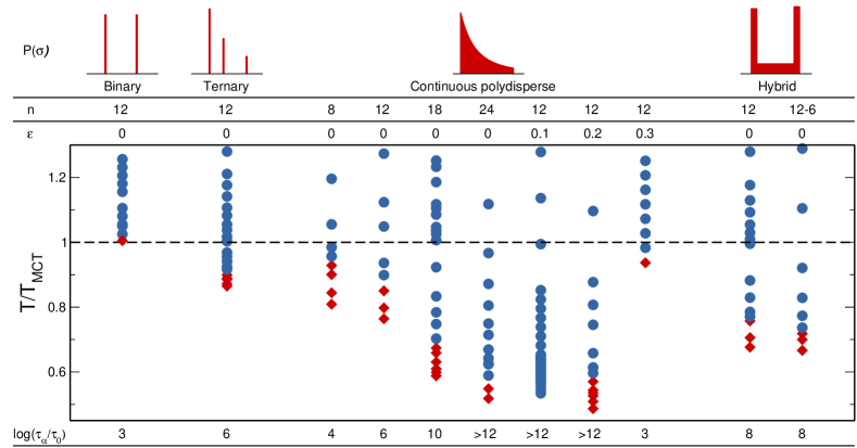
The aim of our work is to bring the swap algorithm to a whole new level of performance. We present a systematic study of glass-forming ability and thermalization efficiency over a broad range of glass-forming models, varying the particle size distribution and the nature of the pair interactions, while optimizing the swap Monte Carlo algorithm. Our main result, summarized in Fig. 1, is the discovery that particular combinations of parameters yield both excellent glass-forming ability and a dramatic decrease of the computer time needed to obtain thermalized configurations at low temperatures. This insight has already led to some new results on related phenomena, such as jamming Berthier et al. (2016a) and the Gardner transition Berthier et al. (2016b).
As shown in Fig. 1, we systematically change the size distribution, using a variety of discrete and continuous mixtures, we vary the softness of the pair repulsion, its additivity, and we add attractive forces. For each case, we determine both the temperature regime where the model is structurally unstable (shown with red symbols) and the temperature regime where the disordered fluid states is stable at equilibrium (shown with blue symbols). The vertical axis represents the temperature , scaled by the location of the corresponding mode-coupling crossover, . Although somewhat arbitrary, this rescaling demonstrates the efficiency of the thermalization because conventional computer simulations typically fail to reach equilibrium in the regime . Despite the differences between systems, several of them can be thermalized in the supercooled liquid state at significantly lower temperatures than ordinary simulations. We demonstrate that this temperature regime corresponds, for some of these models, to a range of relaxation times of more than twelve decades, which implies that we can access in equilibrium a temperature regime that is even lower than the experimental glass transition temperature, . We show that this corresponds to a speed-up of the thermalization of about ten orders of magnitude at .
The two key factors enabling such progress are the use of an appropriate size polydispersity to prevent both crystallization (when polydispersity is too small) and phase separation (when it gets too large), and a particle size distribution that allows for a large acceptance rate for particle swaps, in turn leading to a fast thermalization and equilibrium sampling of phase space.
The outline of the article is as follows. Sec. II is dedicated to the simulation strategy and technicalities. Results for two families of systems (mixtures and continuous polydisperse systems) are reported and discussed respectively in Secs. III and IV. We give a physical insight on swap dynamical relaxation and heterogeneities in Sec. V. Sec. VI deals with the introduction of a model designed to maximize the algorithm efficiency. Finally, Sec. VII presents our conclusions and offers further perspectives for future work.
II Details of the simulations
II.1 Algorithm, interactions and size distributions
We simulate systems of particles in a cubic box of side with periodic boundary conditions Allen and Tildesley (1989). Throughout the paper we will compare results obtained from two kinds of simulation methods: standard Monte Carlo simulations in the canonical ensemble Frenkel and Smit (2001) and swap Monte Carlo simulations Gazzillo and Pastore (1989); Grigera and Parisi (2001). Both simulation algorithms involve the same displacement moves, in which we pick up one particle at random and attempt to translate it by a displacement vector randomly drawn in a cube of linear size . The move is accepted using the Metropolis acceptance rule, which ensures that detailed balance is obeyed at each temperature . For each model, the typical jump length is fixed to a fraction of the average particle diameter, which results in an acceptance rate ranging typically from about 60 at high temperatures to at low temperatures. This approach to simulating glass-formers has been validated by direct comparison with molecular dynamics results for the specific case of a binary mixture Berthier and Kob (2007).
In addition to displacement moves, during a swap Monte Carlo simulation we also attempt to exchange the diameters of two randomly chosen particles. The diameter exchange is again accepted based on the Metropolis criterion. At every Monte Carlo step, such a “swap move” is attempted with probability . We emphasize that swap moves preserve detailed balance and thus guarantee an equilibrium sampling of phase space Newman and Barkema (1999). In other words, despite the “nonphysical” nature of the swap moves (in an experiment, particles would not exchange their diameters spontaneously) the swap Monte Carlo dynamics enables a proper sampling of the equilibrium thermodynamic properties of the model. In previous implementations of the swap Monte Carlo, particle swaps were described as particles exchanging their positions, instead of their diameters Grigera and Parisi (2001). Both descriptions are of course fully equivalent, but our choice offers the advantage that single particle dynamics can be followed in time, because particles do not make arbitrarily large jumps during the swap moves. Standard time correlation functions based on particle displacements can thus be measured in swap and ordinary Monte Carlo simulations in the exact same way. Dynamic measurements are a crucial tool to assess the thermalization of our swap simulations, just as they are for standard simulations of supercooled liquids. One Monte Carlo sweep is then defined as consecutive attempts to either displace or swap particles diameters, and one such sweep will represent in the following our time unit.
In this work we study three different classes of systems, with particle size distributions as sketched in Fig. 1. They are either discrete or continuous mixtures. Discrete mixtures are characterized by a particle size distribution of the form
| (1) |
where is the total number of components, indicates the fractional composition of each species, and is the diameter of species . Within the class of continuously polydisperse systems, we focus on a specific kind of size dispersity, which scales as the inverse of the occupied volume:
| (2) |
where is a normalizing constant and and are the minimum and the maximum diameter values, respectively. This functional form ensures that the volume fraction occupied by particles within a given bin size is constant. Such a scaling property has been shown to enhance glass-forming ability in discrete mixtures Zhang et al. (2015a), but we have not tested this hypothesis in great detail for the present systems.
Finally, we introduce a second type of continuous particle size distributions, which combine the salient features of both discrete and continuous mixtures. For this reason we call them “hybrid” distributions, see Fig. 1. Mathematically, the distributions read
| (3) |
where is the Heaviside function and is defined as before. In this approach each component of the “mixture” is characterized by a flat particle size distribution of width . The goal is to construct models that combine advantages of both discrete mixtures, which are typically good glass-formers, and continuous distributions, for which swap dynamics is very efficient.
We quantify the degree of polydispersity of a system by the normalized root mean square deviation
| (4) |
where the brackets indicate an average of the particle size distribution. In the following, we will use as the unit length for each studied model.
We model the interactions between two particles and via a soft repulsive pair potential of the type
| (5) |
where is an exponent controlling the softness of the repulsive potential, and is a function that smooths the potential at the cutoff distance , beyond which the potential is set to zero. Unless otherwise specified, we use Gutiérrez et al. (2015)
| (6) |
The coefficients , , and ensure the continuity of the potential up to the second derivative at the cutoff distance . Additionally, we also studied a polydisperse model where particles interact with the Lennard-Jones potential
| (7) |
for which we simply cutoff and shift the pair potential at the cutoff distance .
Finally, to ensure a high structural stability in our models, we introduce a generalized non-additive interaction rule for the cross diameters in the pair interaction, which reads
| (8) |
Systems characterized by and will be referred to as additive and non-additive systems, respectively. Non-additivity is another ingredient which has been widely used to enhance glass-forming ability in simple binary models Kob and Andersen (1994) and is a consequence of the band structure of the electronic density of states in metallic alloys Hausleitner and Hafner (1992). Physically, the non-additive rule in Eq. (8) implies that particles with identical diameters interact as before, but that small and large particles can have a larger overlap than for additive systems.
II.2 Physical observables
In this section we introduce the basic observables used to characterize the structure and dynamics of the studied models. We will use them to monitor the equilibration and the stability of the fluids under supercooled conditions and to quantify and compare the degree of thermalization achieved by both standard and swap simulations.
We systematically compute the structure factor Hansen and McDonald (2013),
| (9) |
where is the Fourier transform of the microscopic density at wavevector . The behavior of at small wave-number provides information on possible long-range density fluctuations and will be checked to identify signals of instability of the homogeneous fluid. Since we deal with size-disperse systems, we compute partial structure factors associated to each subpopulation. In the case of continuously polydisperse systems, we group particles of comparable size into families labeled by an index , for which we compute the partial structure factor . A strong increase of at small values is associated to phase separation or demixing, and we have monitored this quantity systematically in our models.
Beside particle demixing, the main instability to be overcome is of course crystallization. To detect the presence of crystalline local order, we measure the 6-fold bond-orientational order parameter Tanaka (2012)
| (10) |
where are spherical harmonics. The sum over runs over the neighbors of particle in a sphere of radius corresponding to the minimum of the distribution function of rescaled inter-particle distances, . We inspect the time and temperature variation of , as well as that of the potential energy , to check whether the systems are stable against crystallization.
We provide a systematic characterization of both self and collective dynamics of the models. This enables us to quantify the degree to which swap simulations enhance thermalization compared to standard Monte Carlo. We note that while standard Monte Carlo dynamics Berthier and Kob (2007) can be used to mimic overdamped Brownian dynamics, as appropriate for a colloidal suspension Brambilla et al. (2009), the microscopic dynamics of swap simulations is not physical. We emphasize however that particles’ trajectories remain well-defined, because the swap moves only exchange the particle diameters, not their positions. Thus, even though the microscopic dynamics is nonphysical, time-dependent correlation functions still quantify the timescale over which individual particles diffuse (for self-correlation functions) and over which the density fluctuations relax (for collective correlations). Time correlation functions will be used in the following to determine whether the system has been efficiently thermalized at a given state point.
We characterize the single particle dynamics through the self-part of the intermediate scattering function
| (11) |
where the wavenumber corresponds to the first peak of the total structure factor . Notice that since the particle diameter changes during the course of the simulations, the sum in Eq. (11) runs over all particles, the distinction between large and small particles being immaterial. The structural relaxation time is then defined as the value at which , following common practice. We use the relaxation time measured for standard Monte Carlo simulations to locate the mode-coupling crossover at , which we take as a relevant temperature scale for computer simulations. In order to obtain we fit the standard dynamics (without swap) in the interval with a power law divergence Götze (2009),
| (12) |
When discussing the dynamics of our models, we will also use other functional forms to describe the temperature evolution of the relaxation time. A well-known functional form is the Vogel-Fulcher-Tamman (VFT) law Berthier and Biroli (2011),
| (13) |
where , and are fitting parameters. Because this functional form describes a dynamic singularity at a finite temperature , it produces a very steep temperature dependence. A less pronounced temperature dependence is obtained with the parabolic law Elmatad et al. (2009),
| (14) |
where , and are again free parameters. Notice that no dynamic singularity is predicted from Eq. (14), since captures the onset of slow dynamics and not the divergence of the relaxation time at low temperature. A final form that we use is the Arrhenius law,
| (15) |
with and two fitting parameters.
Using these functional forms will be useful below to estimate the range of relaxation times that swap dynamics allows us to access. Our analysis shows that the VFT law presumably overestimates the growth of the relaxation time whereas the Arrhenius law underestimates it, the parabolic law falling somewhat in-between. Thus the combination of all three fitting functions provides an estimate of the actual physical behavior and a sensible confidence interval in low temperature extrapolations.
The relaxation of collective density fluctuations is measured via the time-dependent overlap function
| (16) |
using a cutoff distance . This quantity provides similar information as the coherent intermediate scattering function at wavevector , but is computationally more advantageous because it presents much smaller statistical fluctuations. From this function, we define a relaxation time for the decorrelation of collective density fluctuations, such that .
For selected models we computed a number of additional static and dynamical observables with the aim of understanding microscopic processes taking place during the swap Monte Carlo simulations. These more specific observables are described later in Sec. V.
II.3 Efficiency of swap moves
Because the swap Monte Carlo is conceptually very simple, there are very few parameters that can be adjusted to optimize its efficiency. We discuss how to achieve maximal efficiency in the present section.
The extent to which swap moves accelerate the sampling of configuration space during a Monte Carlo simulation must depend on the frequency used to attempt such moves, which is given by the probability . There are two obvious limiting cases. For one recovers the dynamics of a standard Monte Carlo simulation without swap moves. For , instead, only swap moves are attempted and the particle positions are never updated, so that by construction structural relaxation cannot take place. The optimal choice for is thus the one that minimizes the structural relaxation time of the system with respect to .
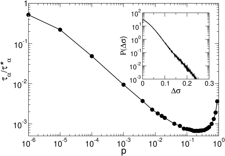
We illustrate the optimisation procedure for a continuously polydisperse particles system interacting via a soft repulsive potential as in Eq. (5) with , with a non-additivity . This model is further discussed in Sec. IV.3. The general trend found for this model is representative of the three classes of systems we investigated and is shown in Fig. 2, where we report the structural relaxation time of the system versus at a constant temperature, . We normalized the relaxation time by the corresponding value in the absence of swap moves at . At this particular temperature, we observe that the structural relaxation time becomes almost three orders of magnitude faster compared to standard dynamics already for very small values of , i.e. of the order of a few percents. We observe a relatively broad minimum around before starts to grow again and diverges for as , when particles stop diffusing for the trivial reason mentioned above. From such a graph, we deduce that is the optimal value for the probability to perform swap moves. We find that this value is fairly robust when temperature is changed or across different models, which presumably stems from the fact that the minimum reported in Fig. 2 is relatively flat. Another remarkable feature of this figure is the very steep decrease of observed for even very small values of suggesting that even a fairly small amount of swap moves is in fact sufficient to facilitate enormously the structural relaxation of the system.
Efficiency considerations should also take into account the CPU time needed to perform a swap move as opposed to a standard displacement. An attempt to swap diameters entails the computation of the local energy variation between the new and the old configuration for two particles, which is twice what is needed for an ordinary displacement move involving only one particle. However, we found that the optimum value for barely changes even when taking this additional effect into account. In terms of CPU time, one MC sweep with takes only longer on average than a standard sweep with . This should be contrasted with the orders of magnitude of gain achieved in terms of structural relaxation time.
Another major advantage of the swap Monte Carlo algorithm is that both its implementation and its efficiency are insensitive to the number of particles in the system, . This contrasts strongly with the replica exchange method, which scales very poorly with Hukushima and Nemoto (1996); Hukushima et al. (1998); Yamamoto and Kob (2000); Odriozola and Berthier (2011).
In general, the acceptance ratio of Monte Carlo moves decreases upon lowering temperature or increasing the density. Similarly, the acceptance ratio of swap moves decreases when the size difference of the two selected particles increases, because a large particle will not easily fit into the hole occupied by a small one. As will be clear in the following, the efficiency of swap moves is highest in continuously polydisperse systems, where the diameter difference between any two particles can be arbitrarily small. In these systems, it is pertinent to avoid attempting exchanges when is too large because the swap move is then essentially always rejected Brumer and Reichman (2004). This point is illustrated in the inset of Fig. 2, where we show , the probability distribution of acceptance rates for swap moves between pairs of particles with a size difference for the same parameters as in the main frame of the figure. We notice that the acceptance rate decays exponentially fast with and becomes vanishingly small when . Following Ref. Brumer and Reichman (2004), we therefore disregard swaps between particles with a diameter difference larger than a certain cutoff. We choose here , which we found to be a reasonable trade-off. We implement this threshold value in a way that preserves detailed balance. In practice, we always choose two particles at random, but we directly reject the swap without evaluating any energy difference if exceeds the chosen cutoff value.
II.4 Equilibration and metastability
Simulations of glass-forming liquids must be long enough to ensure equilibrium sampling of the observables of interest and yet short enough to avoid crystallization or more complex forms of structural ordering. Simple models such as binary mixtures or weakly polydisperse systems have been shown to crystallize over sufficiently long times Brumer and Reichman (2004); Fernández et al. (2010, 2007); Sollich and Wilding (2010a, b); Ingebrigtsen and Tanaka (2015). Computer simulations of glass-forming materials thus always represent a narrow compromise between those two limits that both need to be addressed carefully.
These issues become particularly severe when employing enhanced sampling algorithms, such as swap Monte Carlo moves which are precisely constructed to promote a more efficient exploration of phase space. For instance, crystallization of two-component mixtures of repulsive spheres has been reported in swap Monte Carlo simulations Brumer and Reichman (2004); Fernández et al. (2007); Mártin et al. (2015). The ground-state of polydisperse repulsive particles was studied both with swap Monte Carlo Fernández et al. (2007) and in the semi-grand canonical ensemble Sollich and Wilding (2010a, b). These studies found that for sufficiently high polydispersity the stable structure is a fractionated crystal, where the system presents multiple crystals each involving a fraction of the system overall particle size distribution. However, as noticed in Sollich and Wilding (2010a), the free energy cost of forming an interface between distinct phases is generally high and crystallization may be difficult to observe in practice.
The general conclusion to be drawn from these earlier works is that a model considered as a good glass-forming system when studied using conventional simulations techniques may turn out to be a very poor model when using an enhanced simulation technique that is able to probe a much wider range of temperatures. Indeed, we find that many previously studied types of glass-forming models do not withstand basic stability criteria when the swap technique is applied, forcing us to develop novel numerical models in addition to the optimization of the swap Monte Carlo method.
To make a consistent comparison of the glass-forming ability of the studied models in standard and swap simulations, we follow a rigorous and identical equilibration protocol for all our models. First, we obtain static and dynamical properties of the system by means of standard Metropolis Monte Carlo simulations in the ensemble Frenkel and Smit (2001). From these simulations we extract the average potential energy value, the structure factors and the structural relaxation times. For each model we determine using Eq. (12), which will serve as a reference temperature scale to compare the degree of supercooling across different models. This is not an ideal choice, but it offers the advantage that extrapolation of the relaxation times to low temperatures is not needed.
Swap Monte Carlo simulations start from a configuration equilibrated at the onset temperature Sastry et al. (1998), followed by an instantaneous quench to the target temperature . The following criteria are used to determine whether the system has reached equilibrium at . First, we monitor the potential energy per particle. We inspect both its instantaneous value as a function of time, , to detect aging, as well as its time average as a function of temperature , to detect possible discontinuities or change of slope in the equation of state of the liquid. Second, we ensure that the total mean-squared displacement has reached a value at least larger than . This specific value is relatively immaterial as this criterion only conveniently guides us between state points where particle displacements are large over the numerical time window, from those where particle dynamics is essentially arrested. Finally, we look at the self-incoherent scattering function. For this quantity, we check, within statistical fluctuations, both the absence of aging and the complete decorrelation to zero at long times. Once equilibration has been reached, we perform a first set of simulations to obtain a rough estimate of the structural relaxation time in the presence of swap moves. After this is done, the system is simulated over a total of to measure static and dynamic properties over a sufficiently wide time window. Notice that this thermalization procedure is rather demanding and thermalization thus requires that we are able to perform simulations over a time window which is 2 orders of magnitude longer than the structural relaxation time. We emphasize that such procedure is not specific to the presence of the swap moves. We think that simulation of supercooled liquid should follow similar strict rules to claim that equilibration as well as a proper sampling of phase space has been achieved.
Almost every system we simulated eventually displays some form of structural instability at sufficiently low temperature, such as nucleation of an ordered phase or long wavelength density fluctuations and demixing. These instabilities are detected via the observables introduced in the previous section. To decide whether a given state point remains in a metastable disordered fluid state, we use the following criterion. We perform five independent simulations along the lines described above. If at least one among the five samples shows an instability over a time window of , then we classify this state point as unstable and that the system is a poor glass-former at this temperature. The precise meaning of “instability” is system-dependent and will be specified in each studied case in Secs. III and IV. This criterion is rather strict, as there could still be room for achieving thermalization and performing equilibrium sampling while avoiding structural instability, but this is dangerous as fluctuations related to ordering could interfere with the physics of the metastable disordered state. In addition, we find that when a state point is deemed unstable using our criterion, then lower temperatures are also unstable and the instability rapidly becomes so severe that further studies can not be safely performed. Thus, changing the details of our criterion would simply shift the range of “metastable” temperatures by a very small amount and our conclusions would not be affected.
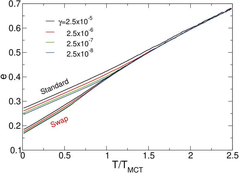
We directly compare the equilibration process between standard and swap simulations in Fig. 3. Starting from a high temperature configuration we progressively quench the system down to zero temperature using a constant cooling rate with values changing logarithmically over a broad interval (. We further average our results using ten independent initial configurations. For standard Monte Carlo simulations, we retrieve the expected behaviour where departure from the equilibrium equation state arises at lower temperature for lower cooling rate, as signalled by a rate dependence of the energy. Using swap simulations, we obtain the very same equation of state at equilibrium, and a similar rate-dependent behaviour at low temperatures. The major difference between the two sets of simulations is that swap simulations clearly fall out of equilibrium at considerably lower temperatures than ordinary Monte Carlo simulations. The agreement of the two sets of curves when they both probe equilibrium is an indication that swap dynamics has been correctly implemented and and provides the correct sampling of phase space. The second information gained from this set of data is the clear indication that the swap Monte Carlo algorithm extends the regime where equilibrium studies are possible by a large amount and is able to produce highly stable glass configurations.
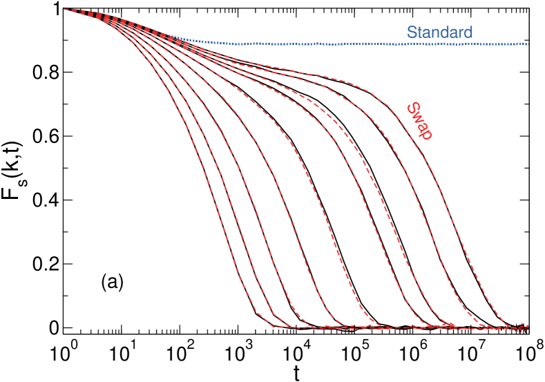
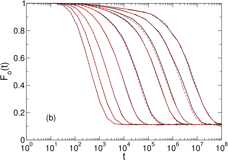
To illustrate our equilibration protocol, we show in Fig. 4(a) the incoherent scattering function for the same system as in Fig. 2 (see also Sec. IV.3) evaluated over the first and the second halves of the simulation at various temperatures. As we can see, the two sets of curves agree within statistical uncertainty over a wide range of temperatures, demonstrating the absence of aging. For the lowest temperature at which thermalization with swap moves is achieved, we show the corresponding relaxation function obtained without swap, which quickly decays to a plateau that extends over the last 6 decades of the simulation. This shows that without swap moves, the dynamics is fully arrested at these low temperatures, and no equilibrium simulations can presently be performed in this regime with conventional computational techniques.
In Fig. 4(b), we show the collective overlap function, Eq. (16), which decorrelates to a density-dependent plateau at long times, as expected in ergodic equilibrium simulations. The two plots of Fig. 4 underline the fact that swap Monte Carlo simulations fully decorrelate both single particle and collective density fluctuations in a regime where standard Monte Carlo simulations may be fully arrested and therefore represent an efficient and reliable method to sample the configuration space.
III Results for discrete mixtures
III.1 Binary mixtures
Simple binary mixtures of repulsive spheres were the first computer models for supercooled liquids simulated using the swap Monte Carlo method Gazzillo and Pastore (1989); Grigera and Parisi (2001). Here, we focus on the “historical” 50:50 binary mixture introduced long ago by Bernu et al. Bernu et al. (1987b), which has been frequently used since its introduction. The pair interaction is given by Eqs. (5) and (8) with and , where are species indexes. The size ratio is , resulting in a polydispersity . The potential is cutoff and shifted at a distance , a specific value which was often used in previous studies Grigera and Parisi (2001); Brumer and Reichman (2004); Mártin et al. (2015). We simulate particles at the number density .
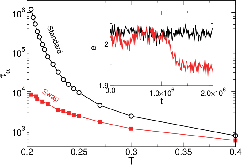
As already demonstrated before Mártin et al. (2015), swap moves help to accelerate sampling in this system, even though their acceptance rates is relatively low, of order . We confirm this finding in Fig. 5 where we compare the structural relaxation time measured during standard and swap Monte Carlo simulations. Over the range of temperatures at which the system can be equilibrated according to our criteria (see Sec. II.4), swap moves result in a speedup of about orders of magnitude at the lowest temperature. Notice that contrary to published analysis Fernández et al. (2006), we find that the efficiency of the swap over the standard Monte Carlo method is strongly temperature-dependent, and efficiency increases rapidly as temperature decreases.
Unfortunately, however, the temperature range that can be analyzed with this system does not change dramatically when swap moves are introduced. In fact, even using standard MC, the system crystallizes at the lowest studied temperature and becomes unstable when , which is marginally larger than the location of the mode-coupling crossover, . Notice that earlier, incorrect determinations of the mode-coupling crossover temperature of this system have misleadingly suggested that temperatures well below could be simulated with this system. In reality, represents the lowest temperature that can be safely studied, swap moves merely providing a more efficient way of producing thermalized configuration in the temperature regime . In other words, swap MC accelerates the dynamics of the system but does not allow the exploration of a temperature regime that is not already accessible with ordinary simulations.
In the inset of Fig. 5 we show the time series of the potential energy of a sample at , where rapid crystallization is observed when swap dynamics is employed. We note that crystallization in this model is well-documented and has been studied in detail in small samples Brumer and Reichman (2004); Berthier et al. (2012). Since complex strategies would be needed to detect and filter out crystallized configurations Mártin et al. (2015) already near the mode-coupling crossover, we conclude that this “historical” model can indeed be efficiently simulated using swap Monte Carlo but is too poor a glass-former to fruitfully explore novel physical regimes.
Within the realm of simple binary mixtures, it is difficult to make further progress using swap Monte Carlo because to increase the structural stability of the system one would need to increase the size ratio (for instance using the more stable well-studied model), but this would imply that the already very low acceptance rate for swap moves would become vanishingly small and swap would thus not be a useful method. Therefore, the trade-off between stability and swap efficiency leaves very little room for a drastic improvement of simulation techniques when binary mixture models of glass-formers are used. Another option is to introduce non-additivity in the interactions, as for instance in the classic Kob-Andersen mixture Kob and Andersen (1994). Rather than for binary mixtures, we will explore this possibility for a different family of models based on continuously polydisperse particles (see Sec. IV).
III.2 A ternary mixture
Given the limits demonstrated above for binary mixtures, a natural strategy is to increase the number of components in the model. Adding more chemical components is indeed a commonly used method to improve the glass-forming ability of metallic alloys. In addition, by increasing the number of components, one can simultaneously increase the polydispersity, and thus the glass-forming ability of the model, while preserving the swap efficiency by introducing particles with size ratios that are small enough for swap moves to be frequently accepted.
This strategy was recently followed in Ref. Gutiérrez et al. (2015), where a ternary mixture of soft spheres was introduced and studied using swap Monte Carlo dynamics. The potential used in that work can be cast in the form of Eq. (5) with a softness parameter and as in Eq. (6), with a cutoff distance . We simulated systems with particles at the number density , as in the original version of the model Gutiérrez et al. (2015). The size ratio between two species is , which is slightly larger than for the binary mixture studied above in Sec. III.1, and compositions , , and , which ensures that all species roughly occupy the same fraction of the total volume. The corresponding size polydispersity is , and so we can expect a smaller tendency for the system to crystallize. Simultaneously, we also expect the acceptance of the swap moves to be much smaller than for the binary mixture. In agreement with Ref. Gutiérrez et al. (2015), we find that the acceptance rate for swaps is of the order at low temperatures. To speed up the simulations, we therefore only attempt swap moves between species and separately, because the probability of accepting swaps between pairs of particles is negligible.
Despite the low acceptance rate, it was claimed in Ref. Gutiérrez et al. (2015) that swap moves allow for a dramatic speedup of the thermalization in this model. In the reduced units described above, we locate the mode-coupling crossover temperature near , and Gutierrez et al. claim to have achieved thermalization down to . Based on dynamic scaling arguments, they estimate that the relaxation time at is , where is the value of the relaxation time near the onset temperature . Thus, the claim is that swap Monte Carlo provides an increase in the accessible window of relaxation times of about 10 orders of magnitude as compared to standard molecular dynamics simulations Gutiérrez et al. (2015).
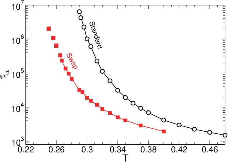
We have repeated and extended these simulations using standard and swap Monte Carlo dynamics. In Fig. 6 we present the temperature evolution of the structural relaxation times for both these dynamics. We confirm that despite the very low acceptance rate of the swap moves, the speedup of the dynamics produced by these rare swaps is important. For instance, at the lowest temperature simulated by standard Monte Carlo, the relaxation time is reduced by a factor of about when swap moves are introduced. Following the evolution of using swap moves, we find however that becomes too large to be accurately measured for and particles in fact barely move over the entire simulation performed at . We conclude therefore that our swap Monte Carlo simulations fail to thermalize the model for . In Ref. Gutiérrez et al. (2015), thermalization was tested by reweighting the probability distribution functions of the potential energy. We could reproduce this thermalization test in our work, thus demonstrating that this test fails to detect the lack of thermalization and proper sampling for the lowest studied temperatures. Measuring the structural relaxation time and the relaxation dynamics is thus a more accurate and more discriminating thermalization test than techniques based on global static observables only.
In addition to the lack of thermalization at low temperatures, we also find signatures of structural instability of the fluid at even higher temperatures, . Below this temperature, our criteria for absence of crystallization or demixing are no longer fulfilled, and the system is eventually unstable within the window of that we use to assess stability. Using shorter time windows before the system crystallizes, we obtain a rough estimate of the relaxation time in the unstable regime, and show these results as disconnected squares in Fig. 6. In Ref. Gutiérrez et al. (2015), the glass-forming ability of the model was not discussed but there may be evidence of ordering in the reported peak of the specific heat. An alternative reason for the absence of ordering in the data of Ref. Gutiérrez et al. (2015) is that the performed simulations covered a smaller time window of about Monte Carlo sweeps, whereas we simulate up to sweeps in our work. Of course, preventing ordering through shorter simulations implies that thermalization becomes more difficult to achieve, and an accurate sampling of phase space is then problematic.
Comparing the stable results for the ternary mixture to the ones of the binary mixture in Fig. 5, it is clear that the efficiency of swap Monte Carlo is essentially preserved, and that thermalization and metastability of the fluid branch have indeed been extended to temperatures below , although the gain is far less spectacular than the one claimed in Ref. Gutiérrez et al. (2015), once thermalization and structural stability are more precisely characterized.
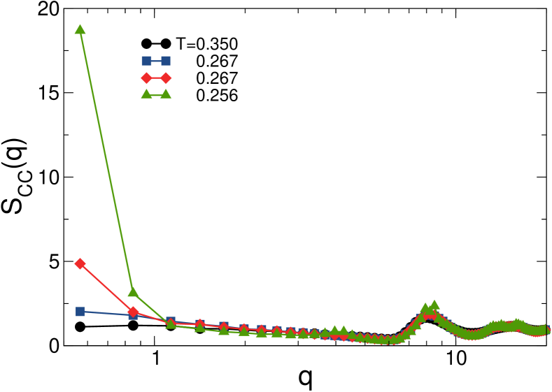
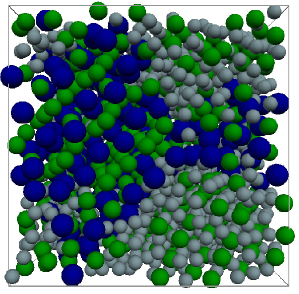
We studied more carefully the structural properties of the ternary mixture using partial structure factors, and we show some representative results in Fig. 7 for at various temperatures. At high temperatures, , we find that the structure factor resembles the one found for ordinary glass-forming models, with a strong first diffraction peak corresponding to the inter-particle distance and a featureless plateau at lower wavevectors. In the low-temperature regime, where swap Monte Carlo is mandatory to achieve thermalization, , we find that increases more strongly as decreases towards 0, which suggests that composition fluctuations are already quite strong in this regime. Even for these state points, which we deemed “stable” based on our stability criterion, longer simulations show that these fluctuations can trigger a demixing in the system, as illustrated for in Fig. 7. We have obtained similarly demixed configurations for temperatures up to , showing that stability is a real issue in this model. Finally, for , the system always demixes within our simulation time, which produces a strong low- peak in the structure factor, see Fig. 7. When the particles are segregated, they then easily crystallize and we obtain configurations such as the ones shown in the inset of Fig. 7. We conclude that maintaining this system in metastable fluid state at low temperatures, , is actually very difficult because (i) thermalization becomes prohibitively difficult and (ii) simulations longer than the thermalization time in this regime produce demixed and ordered configurations.
Finally, to assess more quantitatively the gain in efficiency obtained for this ternary mixture, we have fitted our dynamic relaxation data from standard Monte Carlo simulations to various fitting formula commonly used in the glass literature. Using both a Vogel-Fulcher fit, Eq. (13), which presumably overestimates the data at low , and a parabolic singularity-free formula, Eq. (14), we consistently obtain that the relaxation time at is about . This is two orders of magnitude slower than the lowest temperature simulated without the swap moves, see Fig. 6. At this low temperature , the relaxation time using swap is and so the thermalization speedup due to swap moves is about three orders of magnitude.
Therefore, we confirm that the ternary mixture introduced in Ref. Gutiérrez et al. (2015) can be equilibrated at temperatures below the mode-coupling crossover and we have estimated that this corresponds to an extension of the accessible dynamic regime of about two decades compared to standard simulations. This achievement thus competes favorably with the other computational approaches described in the introduction, but it still does not allow for an exploration of glass physics much closer to the experimental glass transition, which we shall achieve below for continuous polydispersity.
III.3 Five-component mixtures
Because ternary mixtures offered only limited success, we tried to improve both swap move acceptance and the metastability of the liquid phase by performing an exploratory study using two different five-component mixtures. We again adjusted the concentration of the various species so that each component roughly occupies the same volume, and we chose the size ratio between the different families to be small enough that swap moves are accepted with a reasonable acceptance rate.
We studied two systems with diameters roughly linearly spaced between and for a polydispersity , and between and for a polydispersity , Thanks to the reduced size ratio between individual components, the swap acceptance rate increased considerably as compared to the binary and ternary mixtures studied above, and ranges between 10% and 20% depending on temperature. However, both models displayed a strong tendency to demix during swap Monte Carlo simulations and it proved impossible to equilibrate these systems well below following the criteria described above.
We have clearly not exhausted all possible discrete models of glass-formers, as the parameter space becomes very large when the number of components increases. It is possible that some parameter combination provides both a rapid thermalization and a good glass-forming ability, and more work would be needed to explore this hypothesis in a more systematic manner, as done for instance in the context of simplified models of bulk metallic glasses Zhang et al. (2015b).
IV Continuously polydisperse systems
IV.1 Why continuous polydispersity?
The difficulties highlighted in the previous sections arise from the interplay of several competing effects. Reducing the diameter difference between species improves the acceptance of swap moves, and thus accelerates thermalization, but the resulting reduced polydispersity makes the system prone to crystallization. Additionally, we found that simple multi-component mixtures show an important tendency to demixing at low temperature.
To tackle these issues at once, we considered a class of models characterized by a continuous particle size distribution . In such systems, swap moves are more likely to be accepted, because there always exist pairs of particles whose diameters are sufficiently close to one another. We found that the succession of a large number of successful swaps between pairs with similar diameters actually facilitates the thermalization of the system. Physically, the end result is that the diameter of each particle performs a kind of random walk in diameter space. An efficient exploration of the diameter distribution seems to be the key for efficient thermalization, as discussed further below in Sec. V.
In addition, by choosing a sufficiently high degree of polydispersity it may be possible to stabilize the liquid against crystallization and fractionation. Therefore, well-chosen continuous particle size distributions seem able to solve all problems encountered in Sec. III above for discrete mixtures at once.
In this section, we study models in which particles interact via Eq. (5), with the cutoff function given by Eq. (6) and a cut-off distance . We simulate particles at . We also fix the particle size distribution to be of the form given by Eq. (2) and vary parameters such as the pair potential and its additivity. This particle size distribution is controlled by a unique parameter, the size ratio or, equivalently, the size polydispersity . Using insight from preliminary studies on hard sphere systems Berthier et al. (2016a), we fix which implies . This observation is in qualitative agreement with the earlier results of Fernandez et al. Fernández et al. (2007), who simulated repulsive spheres with a flat size dispersion and found an optimal stability for polydispersities in the interval . In these models, the acceptance of swap moves is typically very high, -, and does not change dramatically with temperature.
IV.2 Influence of the particle softness
Our first analysis of models with continuous polydispersity concerns the role of the particle softness. Previous studies have found that softness can have a non-trivial impact on glass properties, such as fragility Michele et al. (2004) and glass-forming ability Zhang et al. (2015a). Here we simulated polydisperse soft particles varying the softness exponent using the values , , , . We focus on a continuously polydisperse model with additive interactions, . In the limit where , the model becomes essentially equivalent to the hard sphere model studied in Ref. Berthier et al. (2016a), which displays excellent stability and efficient thermalization. Therefore, the present family of models appears as the natural extension of these hard sphere results to soft potentials.
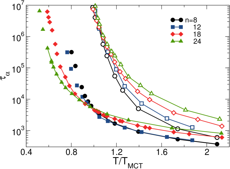
In Fig. 8 we show the structural relaxation times as a function of the temperature for different softness exponents obtained from both standard and swap Monte Carlo simulations. Temperatures are scaled by the corresponding mode-coupling temperature of each model, so that different systems can be represented in the same graph. In all these systems swap moves speed up thermalization significantly. As the exponent increases, i.e. as repulsive forces get steeper, it becomes possible to equilibrate the system at increasingly lower temperatures relative to .
In addition, as for discrete mixtures, the models presented in this section also have a tendency to demix at low temperatures. We have again carefully checked the low- behavior of the partial structure factors that informs us about the presence of large composition fluctuations. Despite the improved stability, we found that the system may still demix at low enough temperatures during the swap Monte Carlo simulations. For these unstable state points, we again use shorter simulations to obtain a rough estimate of the relaxation time, and we show these data using disconnected symbols in Fig. 8. Regarding the structural stability of the models, there is again a clear trend with the softness exponent . We find that softer systems are more prone to structural instability than harder ones. We emphasize that this result is most likely system-specific, since the opposite trend was found in other models of glass-formers Zhang et al. (2015a); Douglass et al. (2016).
Combining the effect of a more efficient thermalization and a better stability of the fluid state, we conclude that models with larger values represent the best choice of parameter within the present family, the system with being stable and efficiently thermalized down to , see Fig. 8. The trend that we find suggests that a system of polydisperse hard spheres with , such as the one recently simulated in Ref. Berthier et al. (2016a), might actually prove the best glass-former in this class of systems with continuous polydispersity, repulsive interactions, and additive interactions.
IV.3 Non-additive interactions
To suppress the tendency to demixing while preserving a continuous form of polydispersity, we have introduced non-additivity in the potential by modifying the sum rule for particle diameters, as described in Eq. (8). Non-additive interactions are known to stabilize the liquid in metallic alloys Zhang et al. (2015a); Kob and Andersen (1994). Moreover, this effect has been demonstrated explicitly in non-additive hard-spheres Gazzillo et al. (1989, 1990). Physically, choosing frustrates phase separation, because particles of different diameters can now stay closer to one another than in the additive case with . To study the effect of non-additivity, we set the softness exponent to and we vary using , and . Note that some results for the case have been already presented in Sec. II above, when discussing the details of the swap algorithm and the thermalization checks.
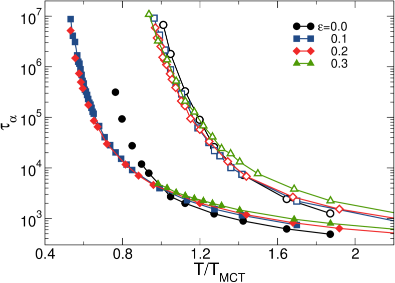
Figure 9 shows the structural relaxation times obtained by varying the degree of non-additivity. As in the previous section, we scale the temperatures by the measured for each model. For comparison, we also redraw the results for the additive system () with . Regarding thermalization efficiency, we find that non-additivity improves the performance of the swap algorithm, as lower temperatures relative to can be studied when , but it is not easy to provide a detailed physical understanding of this result.
Analysis of the low- behavior of the partial structure factors shows that phase separation is strongly suppressed by the non-additivity for both and . At low temperature, however, the system can crystallize, as detected from drops in the time series of the energy and from the appearance of well defined peaks in the structure factor, and we could frequently observe these crystallization events for and . For , the liquid remained stable down to the lowest temperature we could equilibrate with the swap Monte Carlo. This is in fact the only model among the eleven ones studied in this paper that perfectly fulfilled our equilibration and stability criteria throughout the entire accessible temperature range.
The existence of an optimal non-additivity parameter for glass-forming ability presumably results from a competition between demixing, which takes place when , and crystallization, for large . We suggest that the existence of these two distinct paths to ordering actually compete for -, which results in an enhanced frustration and thus a higher structural stability. Similar physical arguments have been proposed in Ref. Zhang et al. (2015b) to explain glass-forming ability of simple non-additive mixtures.
Whereas the additive model with was not the best choice of softness in the previous section, we find that including non-additivity significantly improves both the efficiency of the swap algorithm and the structural stability of this model. We suggest that models with larger (including hard spheres) with non-additive diameters would be even better choices.
It is interesting to contrast the results for the soft repulsion using a continuous size distribution and a non-additivity to the results obtained for the binary mixture in Sec. III.1 for the same pair potential. The conclusion is that the thermalization and stability limits have been decreased from for the binary mixture down to for the present system. This represents a major methodological improvement that we try to quantify in terms of timescales in the next subsection.
IV.4 Experimental timescales are matched by simulations
In the previous section, we showed that by optimizing the additivity and the form of the pair potential, temperatures as low as could be thermalized using swap Monte Carlo in the metastable fluid state. Because ordinary simulations stop near , one may wonder how large is the corresponding gain in terms of structural relaxation times. It is relatively easy to answer this question when the improvement is modest, but this becomes a delicate task in our case, as thermalization is achieved in a temperature regime where the standard dynamics is completely frozen in our observation window and where equilibrium timescales can only be obtained by extrapolation. Extrapolating timescales down to the lowest temperatures where the swap Monte Carlo can thermalize may depend sensitively of the fitting procedure and it therefore requires some care.
We have devised a robust strategy which answers for each model the following question: Is the thermalization speedup due to the swap Monte Carlo algorithm large enough to fill the eight-decade gap between ordinary simulations and experiments? To answer this question for a given model, we employ ordinary Monte Carlo simulations to access a range of relaxation time up to , where represents the value of at the onset of glassy dynamics. In experiments Blochowicz et al. (2005), the glass temperature corresponds to the value , which we will take as our practical definition of . Using the various functional forms described in Sec. II.2, we realized that estimating the location of from numerical measurements of is actually possible with modest uncertainty. More precisely, for a given model we use all three functional forms in Eqs. (13, 14, 15) to estimate the location of from the definition . Despite the qualitative differences between these functional forms, the range of values is reasonably small, typically , with minor variations from one model to the other. Because the VFT law tends to overestimate the increase and the Arrhenius law underestimates it, these two forms respectively provide an upper and a lower bound to the real location of , while estimates from the parabolic law usually fall between those two bounds. Elmatad et al. Elmatad et al. (2009) have shown that the parabolic law accounts for the variation of relaxation times of glass-forming liquids over a broad range of temperatures, ranging from the onset down to the laboratory glass transition. We therefore expect our parabolic extrapolation to provide a reasonable determination of , and the other two temperatures to provide a solid estimate of the interval of confidence.
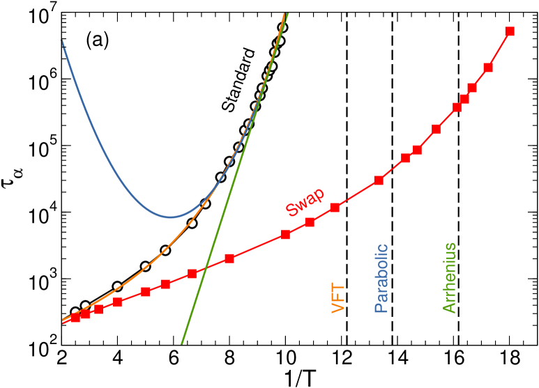
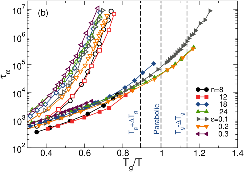
We illustrate this procedure in Fig. 10(a) where we show the temperature evolution of from standard Monte Carlo dynamics for the non-additive model studied in Sec. IV.3, using an Arrhenius representation. We fit these Monte Carlo dynamic data and estimate three different locations for , which delimit the range of possible values for the location of , highlighted with the vertical dashed lines. We then show the evolution of the relaxation time for metastable fluid states when swap Monte Carlo moves are used in the same Arrhenius representation. We find that the swap relaxation time remains modest in the vicinity of , and that this particular system can be thermalized and maintained metastable at temperatures even below the experimental glass temperature . This finding has several important consequences.
-
•
The speedup of the thermalization at is of about 10 () orders of magnitude, implying that computer simulations can now comfortably study that temperature regime in thermal equilibrium.
-
•
The maximal speedup obtained with the swap Monte Carlo is in fact much larger than these 10 orders of magnitude, because temperatures lower than can be thermalized, but estimating that gain becomes very sensitive to the chosen extrapolation.
-
•
For selected models we can now access a temperature regime that even experiments cannot reach, thus opening a novel observational window on the physics of glasses in a regime that has never been probed before, either experimentally or numerically.
To quantify the performance of the swap algorithm, we estimate the range of values for each model studied in this section, and use these fitted values to construct an Angell plot, representing the logarithm of the relaxation times as a function of the scaled inverse temperature, , see Fig. 10(b). In practice, we use the value given by the parabolic which falls in the middle of the fitted range and show the corresponding uncertainty, estimated from VFT and Arrhenius fits, with the vertical dashed lines in Fig. 10(b). Standard Monte Carlo simulations typically stop near -1.5, in the vicinity of the mode-coupling crossover. For most models, the swap algorithm performs so well that the thermalization time at remains modest, . This corresponds to a thermalization speedup at of 10 orders of magnitude. As mentioned before, models with soft potentials and additive interactions are prone to structural instability, and some of them are not stable down to . However for several models, we find that thermalization and fluid metastability can be maintained below .
The discovery of such glass-forming models associated to an efficient algorithm to thermalize them represents the main achievement of our work.
V Microscopic insights into the swap dynamics
V.1 Dynamics of particle diameters
The previous sections demonstrated that swap Monte Carlo moves can enhance thermalization by several orders of magnitude, the effect being most spectacular in continuously polydisperse systems, for which swap moves have a very high acceptance rate. In this section we shed some light on the microscopic mechanisms that are responsible for this acceleration. We carry out this analysis for a non-additive polydisperse model with introduced in Sec. IV.3.
It has been previously suggested that the swap moves increase the particle mobility because they allow the particles to escape the cage formed by their neighbors Grigera and Parisi (2001); Gutiérrez et al. (2015) after a non-local swap move. This view seems correct when one considers that particles exchange their positions, because a caged particle indeed appears to jump instantaneously to a novel position. However, the swapped particle is actually replaced by another particle which is then occupying the caged position itself, and it jumps to a position where another particle was caged too. Therefore, it is not clear that the cage is affected at all after a swap move, and this simple explanation cannot explain the speedup of the dynamics.
This conclusion is more easily grasped when one considers, as we do, that particles simply exchange their diameters during a swap move, without changing position. In that case, the diameter of each caged particle slowly fluctuates in time. For continuous polydisperse systems, these time fluctuations take the form of a random walk in diameter space. Therefore, we conclude that it is rather the slow wandering of the diameter of each particle that allows the system to relax more efficiently towards equilibrium. A naive physical explanation would be that a caged particle with a large diameter could start diffusing by shrinking its radius, thus being able to squeeze and escape through a small channel. We shall now demonstrate that the physics is actually more complicated and more collective than this naive image.
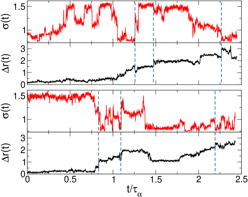
To see this, let us start with some qualitative observations on the time evolution of the diameter of a tagged particle. We show two typical time series of for two different particles in Fig. 11. We rescale the time axis by to better appreciate how much the particle diameter changes over a relaxation time of the system. On short time scales the diameter fluctuates around its initial value, while at longer times it changes and eventually visits all values allowed by the particle size distribution. At low temperature these relaxation events occur suddenly and appear as jumps. Overall, this behavior strongly resembles the typical features of glassy dynamics known from real space analysis of single particle displacements, mimicking very much the cage effect and hopping motion. To reinforce this analogy, we show the time series of the particle displacements for the same two tagged particles in Fig. 11. As expected, they display periods of immobility separated by rapid jumps.
The comparison of the two panels reveals that some of the sudden jumps in diameter space occur at similar times as the sudden jumps of the particle in real space which indicates that diameter dynamics can trigger diffusion. However, we can also detect jumps occurring in real space without clear counterparts in diameter space, and vice versa. These observations suggest that changing the diameter of a single particle is not necessarily enough to trigger a rearrangement, and also that changes in the neighborhood of one particle may be enough to trigger a displacement. Overall, the physical picture is that relaxation in these supercooled states is a collective process and the efficient thermalization with swap cannot be explained on the basis of a simple single-particle argument.
To quantify the correlation between diameter and position dynamics, we define a time correlation associated to the time evolution of the diameters. We define the following auto-correlation function for diameter fluctuations:
| (17) |
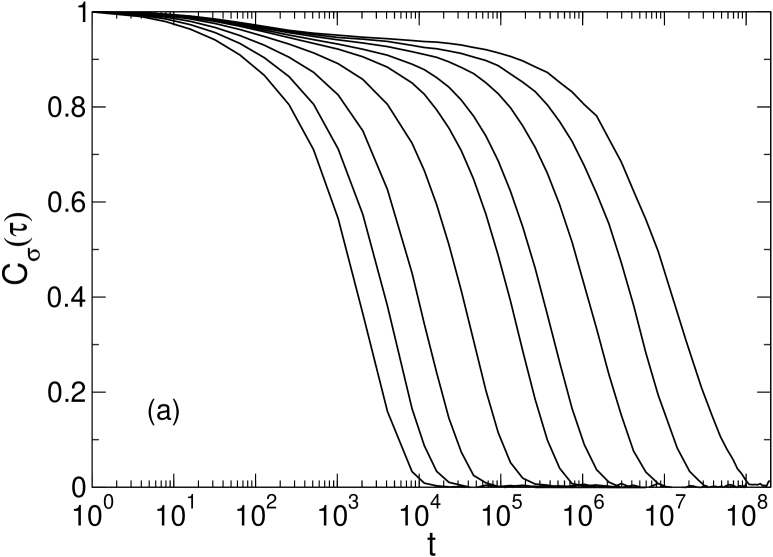
where . This function is normalized so that it evolves from unity when , to zero at large times when diameters become completely uncorrelated from their initial values. The temperature variation of this function is shown in Fig.12(a). By lowering the temperature develops a plateau after an initial short time decay and eventually decorrelates at longer times. This confirms the previous qualitative observations that the diameters remain “caged” around some initial value before complete decorrelation.
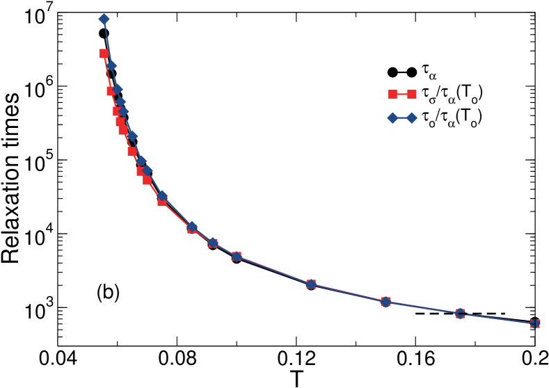
Let us define the diameter decorrelation times as the value of time such that . In Fig. 12(b), we compare the temperature evolution of three different relaxation times for single-particle motion, , for single-particle diameter, , and for collective density fluctuations, . We absorb the observable dependence of these three timescales by rescaling them at a single temperature where the relaxation is fast, namely . The striking result of these measurements is that single particle displacements, density fluctuations and diameter fluctuations all relax on the same timescale. Because diffusion is fully arrested when the diameters do not fluctuate we conclude that it is the efficient dynamics in diameter space which drives the structural relaxation in position space, and therefore, the efficient thermalization of the system.
A further intriguing observation about the role of diameter fluctuations stems from the data shown in Fig. 4, where time correlation functions for standard and swap dynamics are compared at the same very low temperature, where even the swap dynamics is very slow. In that case one observes that the plateau height related to short-time vibrational motion is different in the two dynamics, the amplitude of these vibrations being much larger when the swap dynamics is used. This observation implies that at short times the small fluctuations in particle diameters act as an additional degree of freedom that allows each particle to perform back and forth caged motion over a typical distance that is larger than in the standard dynamics. These larger in-cage fluctuations suggest a possible “softening” of local cages, which seems to correlate well with an acceleration of the dynamics. Such a correlation between short-time motion and structural relaxation is often discussed in the context of glass-forming models Buchenau and Zorn (1992); Scopigno et al. (2003); Dyre (2006); Hansen et al. (2017), and it would be interesting to study it further in the present context.
V.2 Spatially heterogeneous dynamics
The correspondence between the timescales for diameter and position dynamics, accompanied by a lack of strong correlation at the single particle level, suggests that the physics of diffusion in real and diameter space is cooperative in nature. For instance, diffusive events could be happening more easily in a spatial region where the diameter dynamics has been particularly efficient. This hypothesis suggests to investigate the existence of spatial correlations of the dynamical relaxations.
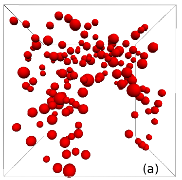
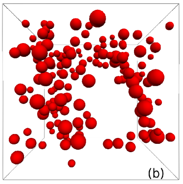
To illustrate this point qualitatively, we show in Fig. 13 two typical configurations at a temperature . We measure the dynamics between an arbitrary initial time and a later time . In Fig. 13(a) we show the particles having the 10 largest displacements in real space over this time lag, whereas in Fig. 13(b) we show the particles having the 10 largest displacements in diameter space. Particles are drawn using rescaled final diameter values. We observe a close similarity between regions of faster diffusing particles and regions of particles with large diameter changes, but we also recognize that the correlation does not hold at the particle level. Thus, we conclude that diameter changes and structural relaxation may affect each other in a non-local fashion.
The spatial correlations of diameter fluctuations can be characterized using the multi-point functions introduced to study cooperative motion in supercooled liquids Toninelli et al. (2005). The generic expression of the dynamical susceptibility related to a time-dependent observable is
| (18) |
It quantifies the extent of spatial correlations associated to the local observable over a time scale Toninelli et al. (2005). Here we measure dynamic susceptibilities associated both to the self-part of density fluctuations, with [see Eq. (11)], and to diameter fluctuations, with [see Eq. (17)]. These functions provide information on the spatially heterogeneous dynamics of particle displacements and of diameter changes, and they typically display a peak around the timescales and , respectively. In Fig. 14 we report the height of these two peaks, and , as a function of the temperature. In addition we also measure and report the behavior of for the standard Monte Carlo dynamics.
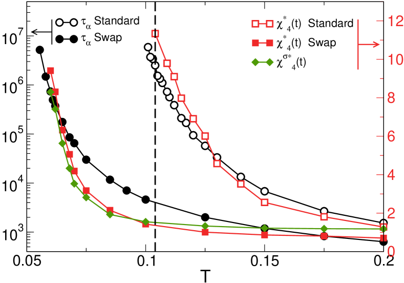
This figure provides two main pieces of information. First, we notice that the temperature dependence of in standard and swap simulations are very different. The behavior for standard Monte Carlo is as reported before Berthier et al. (2007), where increases rapidly from a value when the temperature is decreased below the onset to a value when approaching , in way that mirrors the evolution of the relaxation time , as demonstrated in Fig. 14. The traditional interpretation is that dynamics becomes spatially correlated over larger length-scales as the temperature is lowered. A striking observation is that the swap dynamics near displays essentially no spatial dynamic correlations. By construction, swap moves can affect the dynamics of the system but not its equilibrium static properties. Therefore, we conclude that the growth of the spatial correlations detected by for in standard dynamics is mostly of dynamic, rather than structural, origin. This finding, which agrees qualitatively with previous conclusions Berthier and Jack (2007); Jack et al. (2014), may also explain why the swap algorithm can be very efficient, because if spatial correlations had a strong structural component, then a strong numerical acceleration would likely necessitate the introduction of a more collective algorithm.
The second key information from Fig. 14 is that both quantities and with swap dynamics are quantitatively very close, which confirms that fluctuations in real and in diameter spaces are strongly correlated. Even though the correlation is not strong at the local scale, diameters fluctuations display the same temperature evolution as dynamic heterogeneities. In addition, both quantities follow the growth of the swap relaxation time, the swap algorithm becoming slow at low enough temperatures, at which important spatial correlations of the diameter dynamics become needed to relax to system towards equilibrium.
VI Ideas for the future design of glass-forming models
In this section, we build on the detailed level of understanding of the swap mechanism reached in the previous sections to propose novel directions and ideas to design new glass-forming models for which the swap Monte Carlo approach could be very efficient.
VI.1 “Hybrid” models for binary mixtures
A large number of models studied in the past were based on discrete mixtures Bernu et al. (1987b); Kob and Andersen (1994); Wahnström (1991), as studied in Sec. III. We concluded there that swap was not well-suited for binary mixtures because a large acceptance rate for the swap seems incompatible with a good structural stability. We now show that it is possible to construct models which have the characteristics of binary mixtures, reasonable stability, and can be efficiently simulated using the swap algorithm.
Our idea is to introduce what we call a “hybrid” particle size distribution, as sketched in Fig. 1. These distributions are composed of two main peaks which are a good representation of an binary mixture. In order to have a good glass-forming ability, we choose an equal concentration of particles in these two peaks, and, more importantly, we choose a size ratio which is large enough to avoid the crystallization observed otherwise. Because such a large size ratio implies that swap moves are always rejected, we introduce a third specie in the model, associated to a flat continuous distribution of particle sizes that connects smoothly the two main peaks of the binary mixture. The main idea is that a particle belonging to one of the two main components can be swapped with particles belonging to the intermediate third specie, and it can then slowly tunnel through to reach the other specie. In other words, whereas a direct particle exchange between and is unlikely, the addition of the interpolating specie facilitates such exchanges which can then happen via a large number of intermediate swaps which all have a large acceptance rate.
In practice, we introduce two species () with flat continuous polydispersity around two average diameter values () such that . We add a third specie, , with an average diameter value , which continuously interpolates between small and large diameters. Each specie contains roughly of the particles. The final size distribution is described by Eq. (3) with the chosen parameters , , , , , , , , . The two-body potential is given by Eqs. (5, 6) with and a cut-off distance of . We perform simulations with at . With these parameters, the polydispersity is .
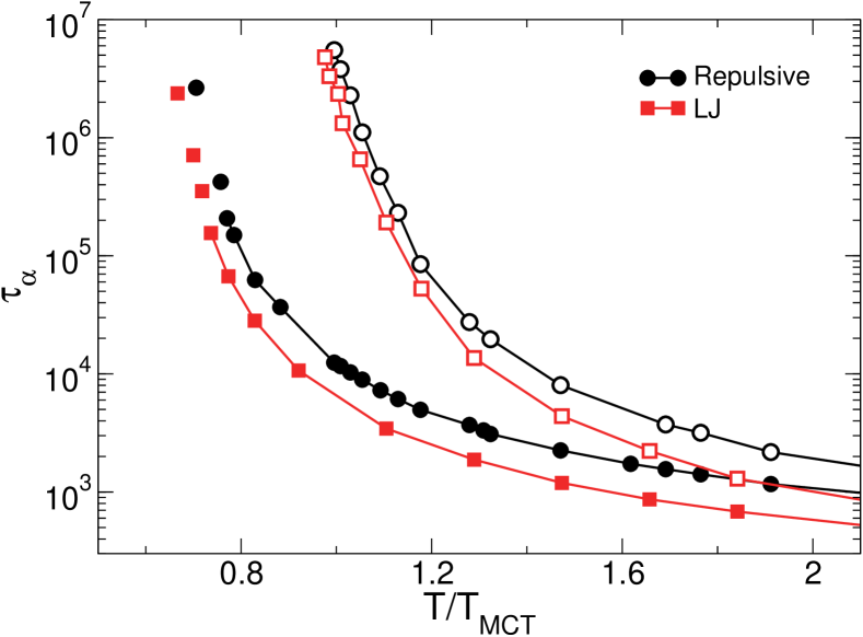
Results for the relaxation times are presented in Fig. 15. As usual, we use disconnected points to represent unstable state points for which short simulations are used to estimate . For this system again, we observe that equilibration is easily attainable for temperatures below , and resistance to ordering is ensured down to relatively low temperatures, . However, at lower temperatures the system again present instabilities due to the tendency to phase separation that we observe through low- values of the structure factor. Preliminary results indicate that using non-additive interactions will most certainly stabilize the system down to even lower temperatures, but the main goal of this section has nevertheless been reached. We have indeed designed a model which is structurally similar to an equimolar binary mixture with size ratio 1.6, but that can be efficiently studied using the swap algorithm down to via the introduction of a third, intermediate specie. Using the same fitting procedure as above, we estimate that these low temperatures allow us to access a total dynamic range of about , so that the swap Monte Carlo method already allows the exploration of a novel temperature regime corresponding to an increase in relaxation times of about 3-4 orders of magnitude as compared to standard Monte Carlo simulations. It would be interesting to study hybrid variants of discrete mixtures, in which the concentration of specie is small enough to be considered as a small perturbation of the original model. Work in this direction is in progress.
VI.2 Lennard-Jones interactions
Up to now, we have studied pair potentials describing repulsive soft spheres with inverse power law repulsion of various softness. However, more realistic pair interactions including attractive forces are often used in studies of supercooled liquids. Perhaps the most studied pair interaction is the Lennard-Jones potential Kob and Andersen (1994), which contains a soft power law repulsion with exponent , combined with a soft power law attraction with exponent , see Eq. (7).
In this final study, we test whether Lennard-Jones interactions can also be efficiently studied using the swap Monte Carlo algorithm. To this end, we start from the previous “hybrid” model studied in Sec. VI.1 and include a power law attraction. Because the potential is now longer-ranged, we use a larger cutoff , and shift the potential by the constant to ensure the continuity of the potential at the cut-off. All other parameters are equal to the ones employed in the hybrid repulsive model above in Sec. VI.1.
We again perform a comparison of the standard and swap dynamics for this Lennard-Jones system, and present the results along the ones of the corresponding repulsive case in Fig. 15. We find that including attractive forces modifies very little both dynamics, apart from a rescaling of the temperature scale: the mode-coupling crossover temperature shifts from 0.680 to 0.543 when including attractive forces Berthier and Tarjus (2011). As a result, the above conclusions regarding stability and thermalization efficiency directly carry out to this Lennard-Jones system. Our main conclusion is therefore that our “feasibility study” is successful and that glass-forming models with Lennard-Jones interactions and a binary-like size distribution can be devised and studied down to very low temperatures using the swap algorithm. Such models will most certainly prove useful in future studies of the glass transition.
VII Perspectives
In this article, we established that a number of glass-forming models with various pair interactions, particle size distributions and degree of non-additivity, can be efficiently simulated using a simple swap Monte Carlo algorithm and remain excellent glass-formers down to very low temperatures. For some models, we have been able to thermalize the metastable fluid down to temperatures that are lower than the laboratory glass transition, which represents the current experimental limit for molecular liquids. Therefore, our paper not only fills the eight orders of magnitude gap between ordinary simulations and experimental work, but it actually goes beyond state-of-the-art experiments and demonstrates that both static and short-time dynamical properties can now be studied in computer simulations in a novel temperature regime. In addition to static quantities, by using thermalised configurations obtained with the swap method as initial conditions for trajectories generated without swap, we believe it is possible to substantially extend the dynamic window for structural relaxation, which may shed new light on the glassy dynamics as well.
Our achievements are summarized in Fig. 1, but throughout the article we have suggested several ways in which our approach could be extended to devise different or more realistic models of glass-forming materials. We have also suggested ways in which the algorithm itself could be improved and described several paths that remain to be explored in future work. We expect these results to trigger a large research activity towards these goals.
Obtaining thermalized states in simple models of supercooled liquids at temperatures comparable to the experimental glass transition paves the way to a number of novel studies, because essentially all simulation work published over the past 30 years could be performed again over a previously inaccessible temperature regime. Some works along these lines have been already published Berthier et al. (2016a, b), and others are currently in progress regarding the thermodynamic properties of deeply supercooled liquids, their local structure, vibrational and mechanical properties, and the existence of a Gardner transition in soft glasses.
Acknowledgements.
We thank G. Biroli, R. Jack, M. Ozawa, I. Procaccia, G. Tarjus, and M. Wyart for useful exchanges about this work. We thank R. Gutierrez for providing additional information regarding simulations performed in Ref. Gutiérrez et al. (2015). The research leading to these results has received funding from the European Research Council under the European Unions Seventh Framework Programme (FP7/2007-2013)/ERC Grant Agreement No. 306845. This work was supported by a grant from the Simons Foundation (# 454933, Ludovic Berthier).References
- Berthier and Biroli (2011) Ludovic Berthier and Giulio Biroli, “Theoretical perspective on the glass transition and amorphous materials,” Rev. Mod. Phys. 83, 587–645 (2011).
- Hunter and Weeks (2012) Gary L. Hunter and Eric R. Weeks, “The physics of the colloidal glass transition,” Rep. Prog. Phys. 75, 066501 (2012).
- Ediger (2000) M. D. Ediger, “Spatially heterogeneous dynamics in supercooled liquids,” Ann. Rev. Phys. Chem. 51, 99 (2000).
- Brambilla et al. (2009) G. Brambilla, D. El Masri, M. Pierno, L. Berthier, L. Cipelletti, G. Petekidis, and A. B. Schofield, “Probing the equilibrium dynamics of colloidal hard spheres above the mode-coupling glass transition,” Phys. Rev. Lett. 102, 085703 (2009).
- Blochowicz et al. (2005) Thomas Blochowicz, Alexander Brodin, and Ernst A. Rössler, “Evolution of the dynamic susceptibility in supercooled liquids and glasses,” in Fractals, Diffusion, and Relaxation in Disordered Complex Systems (Wiley-Blackwell, 2005) pp. 127–256.
- Richert and Angell (1998) R. Richert and C. A. Angell, “Dynamics of glass-forming liquids. V. On the link between molecular dynamics and configurational entropy,” J. Chem. Phys. 108, 9016 (1998).
- Debenedetti and Stillinger (2001) Pablo G. Debenedetti and Frank H. Stillinger, “Supercooled liquids and the glass transition,” Nature 410, 259 (2001).
- Hell (2007) Stefan W. Hell, “Far-field optical nanoscopy,” Science 316, 1153 (2007).
- Ashtekar et al. (2010) Sumit Ashtekar, Gregory Scott, Joseph Lyding, and Martin Gruebele, “Direct Visualization of Two-State Dynamics on Metallic Glass Surfaces Well Below Tg,” J. Phys. Chem. Lett. 1, 1941 (2010).
- Swallen et al. (2007) Stephen F. Swallen, Kenneth L. Kearns, Marie K. Mapes, Yong Seol Kim, Robert J. McMahon, M. D. Ediger, Tian Wu, Lian Yu, and Sushil Satija, “Organic glasses with exceptional thermodynamic and kinetic stability,” Science 315, 353 (2007).
- Barrat et al. (1990) J.-L. Barrat, J.-N. Roux, and J.-P. Hansen, “Diffusion, viscosity and structural slowing down in soft sphere alloys near the kinetic glass transition,” Chem. Phys. 149, 197 (1990).
- Kob and Andersen (1995) Walter Kob and Hans C. Andersen, “Testing mode-coupling theory for a supercooled binary Lennard-Jones mixture. II. Intermediate scattering function and dynamic susceptibility,” Phys. Rev. E 52, 4134–4153 (1995).
- Anderson et al. (2008) Joshua A. Anderson, Chris D. Lorenz, and A. Travesset, “General purpose molecular dynamics simulations fully implemented on graphics processing units,” J. Comp. Phys. 227, 5342 (2008).
- Colberg and Höfling (2011) Peter H. Colberg and Felix Höfling, “Highly accelerated simulations of glassy dynamics using GPUs: Caveats on limited floating-point precision,” Comp. Phys. Commun. 182, 1120 (2011).
- Bailey et al. (2015) Nicholas P. Bailey, Trond S. Ingebrigtsen, Jesper Schmidt Hansen, Arno A. Veldhorst, Lasse Bøhling, Claire A. Lemarchand, Andreas E. Olsen, Andreas K. Bacher, Heine Larsen, Jeppe C. Dyre, and et al., “RUMD: A general purpose molecular dynamics package optimized to utilize GPU hardware down to a few thousand particles,” arXiv:1506.05094 (2015).
- Anderson et al. (2013) Joshua A. Anderson, Eric Jankowski, Thomas L. Grubb, Michael Engel, and Sharon C. Glotzer, “Massively parallel Monte Carlo for many-particle simulations on GPUs,” J. Comp. Phys. 254, 27 (2013).
- Meyer (2013) R. Meyer, “Efficient parallelization of short-range molecular dynamics simulations on many-core systems,” Phys. Rev. E 88, 053309 (2013).
- Newman and Barkema (1999) M. E. J. Newman and G. T. Barkema, Monte Carlo methods in statistical physics (Clarendon Press Oxford University Press, Oxford New York, 1999).
- Dress and Krauth (1995) C. Dress and W. Krauth, “Cluster algorithm for hard spheres and related systems,” J. Phys. A: Math. Gen. 28, L597 (1995).
- Santen and Krauth (2000) Ludger Santen and Werner Krauth, “Absence of thermodynamic phase transition in a model glass former,” Nature 405, 550 (2000).
- Bernard and Krauth (2011) Etienne P. Bernard and Werner Krauth, “Two-step melting in two dimensions: First-order liquid-hexatic transition,” Phys. Rev. Lett. 107, 155704 (2011).
- Swendsen and Wang (1987) Robert H. Swendsen and Jian-Sheng Wang, “Nonuniversal critical dynamics in Monte Carlo simulations,” Phys. Rev. Lett. 58, 86 (1987).
- Binder (1992) Kurt Binder, The Monte-Carlo Methods in Condensed Matter Physics (Springer, Heidelberg, 1992).
- Isobe and Krauth (2015) Masaharu Isobe and Werner Krauth, “Hard-sphere melting and crystallization with event-chain Monte Carlo,” J. Chem. Phys. 143, 084509 (2015).
- Vink (2014) Richard L. C. Vink, “A finite-temperature monte carlo algorithm for network forming materials,” J. Chem. Phys. 140, 104509 (2014).
- Sastry et al. (1998) Srikanth Sastry, Pablo G. Debenedetti, and Frank H. Stillinger, “Signatures of distinct dynamical regimes in the energy landscape of a glass-forming liquid,” Nature 393, 554–557 (1998).
- Hukushima and Nemoto (1996) Koji Hukushima and Koji Nemoto, “Exchange Monte Carlo Method and Application to Spin Glass Simulations,” J. Phys. Soc. Jap. 65, 1604 (1996).
- Hukushima et al. (1998) Koji Hukushima, Hajime Takayama, and Hajime Yoshino, “Exchange Monte Carlo Dynamics in the SK Model,” J. Phys. Soc. Jap. 67, 12 (1998).
- Yamamoto and Kob (2000) Ryoichi Yamamoto and Walter Kob, “Replica-exchange molecular dynamics simulation for supercooled liquids,” Phys. Rev. E 61, 5473 (2000).
- Odriozola and Berthier (2011) Gerardo Odriozola and Ludovic Berthier, “Equilibrium equation of state of a hard sphere binary mixture at very large densities using replica exchange Monte Carlo simulations,” J. Chem. Phys. 134, 054504 (2011).
- Kob and Berthier (2013) Walter Kob and Ludovic Berthier, “Probing a Liquid to Glass Transition in Equilibrium,” Phys. Rev. Lett. 110, 245702 (2013).
- Ozawa et al. (2015) Misaki Ozawa, Walter Kob, Atsushi Ikeda, and Kunimasa Miyazaki, “Equilibrium phase diagram of a randomly pinned glass-former,” Proc. Nat. Acad. Sci. 112, 6914 (2015).
- Berthier (2013) Ludovic Berthier, “Overlap fluctuations in glass-forming liquids,” Phys. Rev. E 88, 022313 (2013).
- Berthier and Jack (2015) Ludovic Berthier and Robert L Jack, “Evidence for a disordered critical point in a glass-forming liquid,” Phys. Rev. Lett. 114, 205701 (2015).
- Faller and de Pablo (2003) Roland Faller and Juan J. de Pablo, “Density of states of a binary Lennard-Jones glass,” J. Chem. Phys. 119, 4405 (2003).
- Callaham and Machta (2017) Jared Callaham and Jonathan Machta, “Population annealing simulations of a binary hard sphere mixture,” arXiv:1701.00263 (2017).
- Gazzillo and Pastore (1989) D. Gazzillo and G. Pastore, “Equation of state for symmetric non-additive hard-sphere fluids: An approximate analytic expression and new Monte Carlo results,” Chem. Phys. Lett. 159, 388 (1989).
- Grigera and Parisi (2001) Tomas S. Grigera and Giorgio Parisi, “Fast Monte Carlo algorithm for supercooled soft spheres,” Phys. Rev. E 63, 045102 (2001).
- Biroli et al. (2008) G. Biroli, J.-P. Bouchaud, A. Cavagna, T. S. Grigera, and P. Verrocchio, “Thermodynamic signature of growing amorphous order in glass-forming liquids,” Nat. Phys. 4, 771 (2008).
- Cammarota et al. (2009) Chiara Cammarota, Andrea Cavagna, Giacomo Gradenigo, Tomas S. Grigera, and Paolo Verrocchio, “Numerical determination of the exponents controlling the relationship between time, length, and temperature in glass-forming liquids,” J. Chem. Phys. 131, 194901 (2009).
- Cammarota et al. (2010) C. Cammarota, A. Cavagna, I. Giardina, G. Gradenigo, T. S. Grigera, G. Parisi, and P. Verrocchio, “Phase-Separation Perspective on Dynamic Heterogeneities in Glass-Forming Liquids,” Phys. Rev. Lett. 105, 055703 (2010).
- Cavagna et al. (2012) Andrea Cavagna, Tomas S. Grigera, and Paolo Verrocchio, “Dynamic relaxation of a liquid cavity under amorphous boundary conditions,” J. Chem. Phys. 136, 204502 (2012).
- Pronk and Frenkel (2004) Sander Pronk and Daan Frenkel, “Melting of polydisperse hard disks,” Phys. Rev. E 69, 066123 (2004).
- Fernández et al. (2007) L. A. Fernández, V. Martín-Mayor, and P. Verrocchio, “Phase Diagram of a Polydisperse Soft-Spheres Model for Liquids and Colloids,” Phys. Rev. Lett. 98, 085702 (2007).
- Fernández et al. (2010) L. A. Fernández, V. Martín-Mayor, B. Seoane, and P. Verrocchio, “Separation and fractionation of order and disorder in highly polydisperse systems,” Phys. Rev. E 82, 021501 (2010).
- Bernu et al. (1987a) B. Bernu, J. P. Hansen, Y. Hiwatari, and G. Pastore, “Soft-sphere model for the glass transition in binary alloys: Pair structure and self-diffusion,” Phys. Rev. A 36, 4891 (1987a).
- Fernández et al. (2006) L. A. Fernández, V. Martín-Mayor, and P. Verrocchio, “Critical behavior of the specific heat in glass formers,” Phys. Rev. E 73, 020501 (2006).
- Brumer and Reichman (2004) Yisroel Brumer and David R. Reichman, “Numerical Investigation of the Entropy Crisis in Model Glass Formers,” J. Phys. Chem. B 108, 6832 (2004).
- Fernández et al. (2007) L. A. Fernández, V. Martín-Mayor, and P. Verrocchio, “Optimized Monte Carlo method for glasses,” Phil. Mag. 87, 581 (2007).
- Santen and Krauth (2001) Ludger Santen and Werner Krauth, “Liquid, Glass and Crystal in Two-dimensional Hard disks,” arxiv:0107459 (2001).
- Gutiérrez et al. (2015) Ricardo Gutiérrez, Smarajit Karmakar, Yoav G Pollack, and Itamar Procaccia, “The static lengthscale characterizing the glass transition at lower temperatures,” EPL (Europhysics Letters) 111, 56009 (2015).
- Berthier et al. (2016a) Ludovic Berthier, Daniele Coslovich, Andrea Ninarello, and Misaki Ozawa, “Equilibrium sampling of hard spheres up to the jamming density and beyond,” Phys. Rev. Lett. 116, 238002 (2016a).
- Berthier et al. (2016b) Ludovic Berthier, Patrick Charbonneau, Yuliang Jin, Giorgio Parisi, Beatriz Seoane, and Francesco Zamponi, “Growing timescales and lengthscales characterizing vibrations of amorphous solids,” Proc. Nat. Acad. Sci. 113, 8397 (2016b).
- Allen and Tildesley (1989) M. P. Allen and D. J. Tildesley, Computer simulation of liquids (Clarendon Press Oxford University Press, Oxford England New York, 1989).
- Frenkel and Smit (2001) D. Frenkel and B. Smit, Understanding Molecular Simulation (Academic, New York, 2nd Ed., 2001).
- Berthier and Kob (2007) L. Berthier and W. Kob, “The Monte Carlo dynamics of a binary Lennard-Jones glass-forming mixture,” J. Phys.: Condens. Matter 19, 205130 (2007).
- Zhang et al. (2015a) Kai Zhang, Meng Fan, Yanhui Liu, Jan Schroers, Mark D. Shattuck, and Corey S. O’Hern, “Beyond packing of hard spheres: The effects of core softness, non-additivity, intermediate-range repulsion, and many-body interactions on the glass-forming ability of bulk metallic glasses,” J. Chem. Phys. 143, 184502 (2015a).
- Kob and Andersen (1994) Walter Kob and Hans C. Andersen, “Scaling behavior in the beta-relaxation regime of a supercooled lennard-jones mixture,” Phys. Rev. Lett. 73, 1376 (1994).
- Hausleitner and Hafner (1992) Ch. Hausleitner and J. Hafner, “Hybridized nearly-free-electron tight-binding-bond approach to interatomic forces in disordered transition-metal alloys. i. theory,” Phys. Rev. B 45, 115 (1992).
- Hansen and McDonald (2013) J. P. Hansen and I. R. McDonald, Theory of simple liquids : with applications to soft matter (Academic Press, Amsterdam Boston, 2013).
- Tanaka (2012) Hajime Tanaka, “Bond orientational order in liquids: Towards a unified description of water-like anomalies, liquid-liquid transition, glass transition, and crystallization,” Eur. Phys. J. E 35 (2012), 10.1140/epje/i2012-12113-y.
- Götze (2009) Wolfgang Götze, Complex dynamics of glass-forming liquids : a mode-coupling theory (Oxford University Press, Oxford New York, 2009).
- Elmatad et al. (2009) Yael S. Elmatad, David Chandler, and Juan P. Garrahan, “Corresponding states of structural glass formers,” J. Phys. Chem. B 113, 5563–5567 (2009).
- Sollich and Wilding (2010a) P. Sollich and N. B. Wilding, “Phase behaviour of polydisperse spheres: simulation strategies and an application to the freezing transition,” J. Chem. Phys. 133, 224102 (2010a).
- Sollich and Wilding (2010b) Peter Sollich and Nigel B. Wilding, “Crystalline Phases of Polydisperse Spheres,” Phys. Rev. Lett. 104, 118302 (2010b).
- Ingebrigtsen and Tanaka (2015) Trond S. Ingebrigtsen and Hajime Tanaka, “Effect of size polydispersity on the nature of lennard-jones liquids,” J. Phys. Chem. B 119, 11052–11062 (2015).
- Mártin et al. (2015) Daniel A. Mártin, Andrea Cavagna, and Tomás S. Grigera, “Specific Heat Anomaly in a Supercooled Liquid with Amorphous Boundary Conditions,” Phys. Rev. Lett. 114, 225901 (2015).
- Bernu et al. (1987b) B. Bernu, J. P. Hansen, Y. Hiwatari, and G. Pastore, “Soft-sphere model for the glass transition in binary alloys: Pair structure and self-diffusion,” Phys. Rev. A 36, 4891–4903 (1987b).
- Berthier et al. (2012) Ludovic Berthier, Giulio Biroli, Daniele Coslovich, Walter Kob, and Cristina Toninelli, “Finite-size effects in the dynamics of glass-forming liquids,” Phys. Rev. E 86 (2012).
- Zhang et al. (2015b) Kai Zhang, Bradley Dice, Yanhui Liu, Jan Schroers, Mark D. Shattuck, and Corey S. O’Hern, “On the origin of multi-component bulk metallic glasses: Atomic size mismatches and de-mixing,” J. Chem. Phys. 143, 054501 (2015b).
- Michele et al. (2004) Cristiano De Michele, Francesco Sciortino, and Antonio Coniglio, “Scaling in soft spheres: fragility invariance on the repulsive potential softness,” J. Phys.: Condens. Matter 16, L489 (2004).
- Douglass et al. (2016) Ian Douglass, Toby Hudson, and Peter Harrowell, “Density and glass forming ability in amorphous atomic alloys: the role of the particle softness,” J. Chem. Phys. 144, 144502 (2016).
- Gazzillo et al. (1989) D. Gazzillo, G. Pastore, and S. Enzo, “Chemical short-range order in amorphous Ni-Ti alloys: an integral equation approach with a non-additive hard-sphere model,” J. Phys.: Condens. Matter 1, 3469 (1989).
- Gazzillo et al. (1990) D Gazzillo, G Pastore, and R Frattini, “The role of excluded volume effects on the structure and chemical short-range order of Ni33Y67 metallic glass,” J. Phys.: Condens. Matter 2, 8463 (1990).
- Buchenau and Zorn (1992) U. Buchenau and R. Zorn, “A relation between fast and slow motions in glassy and liquid selenium,” EPL (Europhysics Letters) 18, 523 (1992).
- Scopigno et al. (2003) T. Scopigno, G. Ruocco, Francesco Sette, and Giulio Monaco, “Is the fragility of a liquid embedded in the properties of its glass?” Science 302, 849–852 (2003).
- Dyre (2006) Jeppe C. Dyre, “Colloquium: The glass transition and elastic models of glass-forming liquids,” Rev. Mod. Phys. 78, 953–972 (2006).
- Hansen et al. (2017) Henriette W. Hansen, Bernhard Frick, Tina Hecksher, Jeppe C. Dyre, and Kristine Niss, “Connection between fragility, mean-squared displacement, and shear modulus in two van der waals bonded glass-forming liquids,” Phys. Rev. B 95, 104202 (2017).
- Toninelli et al. (2005) Cristina Toninelli, Matthieu Wyart, Ludovic Berthier, Giulio Biroli, and Jean-Philippe Bouchaud, “Dynamical susceptibility of glass formers: Contrasting the predictions of theoretical scenarios,” Phys. Rev. E 71, 041505 (2005).
- Berthier et al. (2007) L. Berthier, G. Biroli, J.-P. Bouchaud, W. Kob, K. Miyazaki, and D. R. Reichman, “Spontaneous and induced dynamic fluctuations in glass formers. I. General results and dependence on ensemble and dynamics,” J. Chem. Phys. 126, 184503 (2007).
- Berthier and Jack (2007) Ludovic Berthier and Robert L. Jack, “Structure and dynamics of glass formers: Predictability at large length scales,” Phys. Rev. E 76, 041509 (2007).
- Jack et al. (2014) Robert L. Jack, Andrew J. Dunleavy, and C. Patrick Royall, “Information-theoretic measurements of coupling between structure and dynamics in glass formers,” Phys. Rev. Lett. 113, 095703 (2014).
- Wahnström (1991) Göran Wahnström, “Molecular-dynamics study of a supercooled two-component Lennard-Jones system,” Phys. Rev. A 44, 3752 (1991).
- Berthier and Tarjus (2011) Ludovic Berthier and Gilles Tarjus, “The role of attractive forces in viscous liquids,” J. Chem. Phys. 134, 214503 (2011).