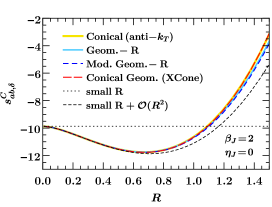
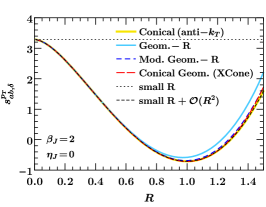
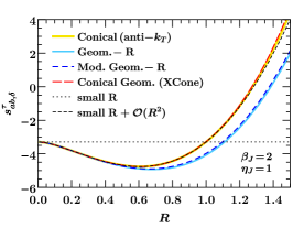
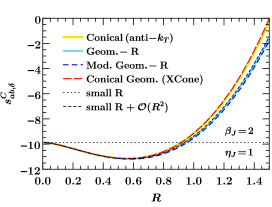
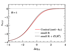
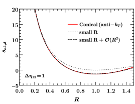
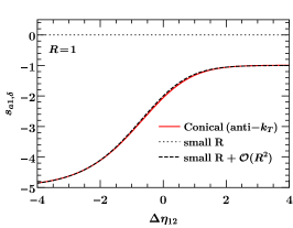
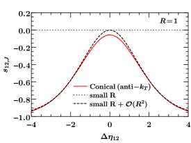
aainstitutetext: Berkeley Center for Theoretical Physics, University of California, Berkeley, CA 94270, U.S.A.bbinstitutetext: Theoretical Physics Group, Lawrence Berkeley National Laboratory, Berkeley, CA 94720, U.S.A.ccinstitutetext: Center for Theoretical Physics, Massachusetts Institute of Technology, Cambridge, MA 02139, U.S.A.ddinstitutetext: Theoretical Division, Los Alamos National Laboratory, Los Alamos, NM 87545, USAeeinstitutetext: Theory Group, Deutsches Elektronen-Synchrotron (DESY), D-22607 Hamburg, Germanyffinstitutetext: Institute for Theoretical Physics Amsterdam and Delta Institute for Theoretical Physics, University of Amsterdam, Science Park 904, 1098 XH Amsterdam, The Netherlandsgginstitutetext: Nikhef, Theory Group, Science Park 105, 1098 XG, Amsterdam, The Netherlands

Soft Functions for Generic Jet Algorithms and Observables at Hadron Colliders

Daniele Bertolini c    Daniel Kolodrubetz c,d    Duff Neill e    Piotr Pietrulewicz c                                        Iain W. Stewart e    Frank J. Tackmann f,g    and Wouter J. Waalewijn dbertolini@lbl.gov dkolodru@mit.edu duff.neill@gmail.com piotr.pietrulewicz@desy.de iains@mit.edu frank.tackmann@desy.de w.j.waalewijn@uva.nl
Abstract

We introduce a method to compute one-loop soft functions for exclusive N𝑁N-jet processes at hadron colliders, allowing for different definitions of the algorithm that determines the jet regions and of the measurements in those regions. In particular, we generalize the N𝑁N-jettiness hemisphere decomposition of ref. Jouttenus:2011wh in a manner that separates the dependence on the jet boundary from the observables measured inside the jet and beam regions. Results are given for several factorizable jet definitions, including anti-kTsubscript𝑘𝑇k_{T}, XCone, and other geometric partitionings. We calculate explicitly the soft functions for angularity measurements, including jet mass and jet broadening, in ppL+1𝑝𝑝𝐿1pp\to L+1 jet and explore the differences for various jet vetoes and algorithms. This includes a consistent treatment of rapidity divergences when applicable. We also compute analytic results for these soft functions in an expansion for a small jet radius R𝑅R. We find that the small-R𝑅R results, including corrections up to 𝒪(R2)𝒪superscript𝑅2\mathcal{O}(R^{2}), accurately capture the full behavior over a large range of R𝑅R.

preprint: DESY 16-137 MIT–CTP 4823 NIKHEF 2016-035  – 23:22

1 Introduction

Exclusive jet processes, i.e. those with a fixed number of hard signal jets in the final state, play a crucial role in the Large Hadron Collider (LHC) physics program. Many important processes, such as Higgs or W/Z𝑊𝑍W/Z boson production or diboson production, are measured in different exclusive jet bins. Furthermore, jet substructure techniques have become increasingly important both in Standard Model and in new physics analyses, and the associated observables often exploit the properties of a fixed number of subjets. Theoretical predictions at increasingly high precision are needed to match the increasing precision of the data. Compared to color-singlet final states, the presence of jets makes perturbative QCD calculations more challenging and the singularity structure more complicated. Furthermore, a fixed number of jets is imposed through a jet veto, which restricts the phase space for additional collinear and soft emissions, and generates large logarithms that often need to be resummed to obtain predictions with the best possible precision.

Soft Collinear Effective Theory (SCET) Bauer:2000ew ; Bauer:2000yr ; Bauer:2001ct ; Bauer:2001yt provides a framework to systematically carry out the resummation of logarithms to higher orders by factorizing the cross section into hard, collinear, and soft functions, and then exploiting their renormalization group evolution. Schematically, the cross section for ppN jets𝑝𝑝𝑁 jetspp\to N\text{ jets} factorizes for many observables in the singular limit as

σN=HN×[BaBbi=1NJi]SN,subscript𝜎𝑁tensor-productsubscript𝐻𝑁delimited-[]subscript𝐵𝑎subscript𝐵𝑏superscriptsubscriptproduct𝑖1𝑁subscript𝐽𝑖subscript𝑆𝑁\displaystyle\sigma_{N}=H_{N}\times\left[B_{a}B_{b}\prod_{i=1}^{N}J_{i}\right]\otimes S_{N}, (1)

where the hard function HNsubscript𝐻𝑁H_{N} contains the virtual corrections to the partonic hard scattering process, the beam functions Ba,bsubscript𝐵𝑎𝑏B_{a,b} contain parton distribution functions and describe collinear initial-state radiation. The jet functions Jisubscript𝐽𝑖J_{i} describe final-state radiation collinear to the direction of the hard partons, and the soft function SNsubscript𝑆𝑁S_{N} describes wide-angle soft radiation. The resummation of large logarithms is achieved by evaluating each component at its natural scale and then renormalization-group evolving all components to a common scale. For an interesting class of observables, the jet and beam functions are of the inclusive type and do not depend on the precise definition of the jet regions. They are known for a variety of jet and beam measurements, typically at one loop or beyond Bauer:2003pi ; Fleming:2003gt ; Becher:2006qw ; Becher:2009th ; Becher:2010pd ; Larkoski:2014uqa ; Stewart:2010qs ; Berger:2010xi ; Becher:2010tm ; Becher:2012qa ; Chiu:2012ir ; Gehrmann:2014yya ; Gaunt:2014xga ; Gaunt:2014cfa ; Luebbert:2016itl . Hard functions are also known for many processes at one loop or beyond (see e.g. ref. Moult:2015aoa and references therein). In this paper, we focus on determining the soft functions that appear for a wide class of jet algorithms and jet measurements. The resummation at NLL and NNLL requires the soft function at one loop. Compared to the beam and jet functions, the perturbative calculation of the soft function generally requires a more sophisticated setup, since it depends not only on the measurements made in the jet and beam regions, but also on the angles between all jet and beam directions and the precise definition of the jet boundaries.

N𝑁N-jettiness Stewart:2010tn is a global event shape that allows one to define exclusive N𝑁N-jet cross sections in a manner that is particularly suitable for higher-order analytic resummation. The calculation of the one-loop soft function for exclusive N𝑁N-jet processes using N𝑁N-jettiness has been carried out for arbitrary N𝑁N in ref. Jouttenus:2011wh . There, N𝑁N-jettiness is used both as the algorithm to partition the phase space into jet and beam regions and as the measurement performed on those regions. To simplify the calculation, the version of N𝑁N-jettiness used in ref. Jouttenus:2011wh was taken to be linear in the constituent four-momenta piμsubscriptsuperscript𝑝𝜇𝑖p^{\mu}_{i},

thrust-like N-jettiness:𝒯Nthrust-like N-jettiness:subscript𝒯𝑁\displaystyle\text{thrust-like $N$-jettiness:}\qquad{\mathcal{T}}_{N} =iminm{2qmpiQm}=iminm{nmpiρm}.absentsubscript𝑖subscript𝑚2subscript𝑞𝑚subscript𝑝𝑖subscript𝑄𝑚subscript𝑖subscript𝑚subscript𝑛𝑚subscript𝑝𝑖subscript𝜌𝑚\displaystyle=\sum_{i}\min_{m}\left\{\frac{2q_{m}\cdot p_{i}}{Q_{m}}\right\}=\sum_{i}\min_{m}\left\{\frac{n_{m}\cdot p_{i}}{\rho_{m}}\right\}\,. (2)

This is essentially a generalization of beam thrust Stewart:2009yx to the case of N𝑁N jets. In eq. (2) the sum runs over the four-momenta piμsubscriptsuperscript𝑝𝜇𝑖p^{\mu}_{i} of all particles that are part of the hadronic final state, and the minimization over m𝑚m runs over the beams and N𝑁N jets identified by the reference momenta qmμ=Emnmμsubscriptsuperscript𝑞𝜇𝑚subscript𝐸𝑚superscriptsubscript𝑛𝑚𝜇q^{\mu}_{m}=E_{m}n_{m}^{\mu} or lightlike vectors nmμ=(1,n^m)superscriptsubscript𝑛𝑚𝜇1subscript^𝑛𝑚n_{m}^{\mu}=(1,\hat{n}_{m}), where Emsubscript𝐸𝑚E_{m} is the jet energy. The directions n^msubscript^𝑛𝑚\hat{n}_{m} for the beams are fixed along the beam axis and for the jets are predetermined by a suitable procedure. Finally, the Qmsubscript𝑄𝑚Q_{m} or ρm=Qm/(2Em)subscript𝜌𝑚subscript𝑄𝑚2subscript𝐸𝑚\rho_{m}=Q_{m}/(2E_{m}) are dimension-one or dimension-zero measure factors. The minimization in eq. (2) assigns each particle to one of the axes, thus partitioning the phase space into N𝑁N jet regions and 222 beam regions. This definition of N𝑁N-jettiness depends only on the choices of jet directions n^msubscript^𝑛𝑚\hat{n}_{m} and measure factors ρmsubscript𝜌𝑚\rho_{m}, which determine the precise partitioning and in particular the size of the jet and beam regions. For the cross section with a measurement of 𝒯Nsubscript𝒯𝑁{\mathcal{T}}_{N}, the 𝒯N0subscript𝒯𝑁0{\mathcal{T}}_{N}\to 0 singular region is fully described by a factorization formula of the form in eq. (1) with inclusive jet and beam functions Stewart:2009yx ; Stewart:2010tn . As 𝒯N0subscript𝒯𝑁0{\mathcal{T}}_{N}\to 0, different choices of jet axes often differ only by power-suppressed effects in the cross section.

N𝑁N-jettiness can also be used more generally as a means of defining an exclusive jet algorithm, which partitions the particles in an event into a beam region and a fixed number of N𝑁N jet regions Stewart:2010tn ; Thaler:2011gf . Here particle i𝑖i is assigned to region m𝑚m for which some generic distance measure dm(pi)subscript𝑑𝑚subscript𝑝𝑖d_{m}(p_{i}) is minimal. These regions are defined by

regionm={particlesi:wheredm(pi)<dj(pi)for alljm}.region𝑚conditional-setparticles𝑖wheresubscript𝑑𝑚subscript𝑝𝑖subscript𝑑𝑗subscript𝑝𝑖for all𝑗𝑚\text{region}\ m=\bigl{\{}\text{particles}\ i:\ \text{where}\ d_{m}(p_{i})<d_{j}(p_{i})\ \text{for all}\ j\neq m\bigr{\}}\,. (3)

This partitioning can be obtained from a generalized version of N𝑁N-jettiness defined by

𝒯N({n^m})=ipTimin{d1(pi),,dN(pi),da(pi),db(pi)}.subscript𝒯𝑁subscript^𝑛𝑚subscript𝑖subscript𝑝𝑇𝑖subscript𝑑1subscript𝑝𝑖subscript𝑑𝑁subscript𝑝𝑖subscript𝑑𝑎subscript𝑝𝑖subscript𝑑𝑏subscript𝑝𝑖{\mathcal{T}}_{N}(\{\hat{n}_{m}\})=\sum_{i}p_{Ti}\min\bigl{\{}d_{1}(p_{i}),\ldots,d_{N}(p_{i}),d_{a}(p_{i}),d_{b}(p_{i})\bigr{\}}\,. (4)

Here the dmsubscript𝑑𝑚d_{m} jet measures depend on pre-defined jet axis n^msubscript^𝑛𝑚\hat{n}_{m}, while the beam measures dasubscript𝑑𝑎d_{a} and dbsubscript𝑑𝑏d_{b} are defined with fixed beam axes along ±z^plus-or-minus^𝑧\pm\hat{z}. Infrared safety requires that all particles in the vicinity of the axis nmμ=(1,n^m)superscriptsubscript𝑛𝑚𝜇1subscript^𝑛𝑚n_{m}^{\mu}=(1,\hat{n}_{m}) are assigned to the respective m𝑚mth region. More precisely the measures have to satisfy dm(pi)<dj(pi)subscript𝑑𝑚subscript𝑝𝑖subscript𝑑𝑗subscript𝑝𝑖d_{m}(p_{i})<d_{j}(p_{i}) for all jm𝑗𝑚j\neq m in the limit piμEinmμsubscriptsuperscript𝑝𝜇𝑖subscript𝐸𝑖subscriptsuperscript𝑛𝜇𝑚p^{\mu}_{i}\to E_{i}n^{\mu}_{m}. Different choices of the dmsubscript𝑑𝑚d_{m} correspond to different N𝑁N-jettiness partitionings, and include for example the Geometric, Conical, and XCone measures Stewart:2010tn ; Jouttenus:2011wh ; Jouttenus:2013hs ; Thaler:2010tr ; Stewart:2015waa . The measure in eq. (2) corresponds to taking pTidm(pi)=(nmpi)/ρmsubscript𝑝𝑇𝑖subscript𝑑𝑚subscript𝑝𝑖subscript𝑛𝑚subscript𝑝𝑖subscript𝜌𝑚p_{Ti}d_{m}(p_{i})=(n_{m}\cdot p_{i})/\rho_{m}. The two beam regions can be combined into a single one by defining the common beam measure

d0(pi)=min{da(pi),db(pi)}.subscript𝑑0subscript𝑝𝑖subscript𝑑𝑎subscript𝑝𝑖subscript𝑑𝑏subscript𝑝𝑖d_{0}(p_{i})=\min\{d_{a}(p_{i}),d_{b}(p_{i})\}\,. (5)

Given a common beam region with a single beam measure d0(pi)subscript𝑑0subscript𝑝𝑖d_{0}(p_{i}), we can always divide it into two separate beam regions for η>0𝜂0\eta>0 and η<0𝜂0\eta<0 by taking for example da(pi)=[1+θ(ηi)]d0(pi)subscript𝑑𝑎subscript𝑝𝑖delimited-[]1𝜃subscript𝜂𝑖subscript𝑑0subscript𝑝𝑖d_{a}(p_{i})=[1+\theta(-\eta_{i})]d_{0}(p_{i}) and db(pi)=[1+θ(ηi)]d0(pi)subscript𝑑𝑏subscript𝑝𝑖delimited-[]1𝜃subscript𝜂𝑖subscript𝑑0subscript𝑝𝑖d_{b}(p_{i})=[1+\theta(\eta_{i})]d_{0}(p_{i}).

Constructing a full jet algorithm requires in addition to the partitioning an infrared-safe method to determine the jet axes n^msubscript^𝑛𝑚\hat{n}_{m}. This could be done by simply taking the directions of the N𝑁N hardest jets obtained from a different (inclusive) jet algorithm. For a standalone N𝑁N-jettiness based jet algorithm, the axes can be obtained by minimizing N𝑁N-jettiness itself over all possible axes,

𝒯N=minn^1,,n^N𝒯N({n^m}),subscript𝒯𝑁subscriptsubscript^𝑛1subscript^𝑛𝑁subscript𝒯𝑁subscript^𝑛𝑚{\mathcal{T}}_{N}=\min_{\hat{n}_{1},\ldots,\hat{n}_{N}}{\mathcal{T}}_{N}(\{\hat{n}_{m}\})\,, (6)

as in refs. Thaler:2011gf ; Stewart:2015waa .

For the calculations in this paper, we consider a very general set of distance measures for determining the partitioning into jet and beam regions as in eq. (4), and a different set of fairly general infrared safe observables measured on these regions. We explore and compare properties of different jet partitionings in sec. 2.2. For the measured observables we consider the generic version of N𝑁N-jettiness variables, 𝒯(m)superscript𝒯𝑚{\mathcal{T}}^{(m)}, given by

𝒯(m)=iregionmfm(ηi,ϕi)pTi.superscript𝒯𝑚subscript𝑖region𝑚subscript𝑓𝑚subscript𝜂𝑖subscriptitalic-ϕ𝑖subscript𝑝𝑇𝑖{\mathcal{T}}^{(m)}=\sum_{i\in\,{\rm region}\,m}f_{m}(\eta_{i},\phi_{i})\,p_{Ti}\,. (7)

Here, ηisubscript𝜂𝑖\eta_{i}, ϕisubscriptitalic-ϕ𝑖\phi_{i}, and pTisubscript𝑝𝑇𝑖p_{Ti} denote the pseudorapidity, azimuthal angle, and transverse momentum of particle i𝑖i in region m𝑚m. The dimensionless functions fmsubscript𝑓𝑚f_{m} encode the angular dependence of the observable and in the collinear limit behave like an angularity, see sec. 2.1. When considering a single beam region we have a common beam measurement 𝒯(0)=𝒯(a)+𝒯(b)superscript𝒯0superscript𝒯𝑎superscript𝒯𝑏{\mathcal{T}}^{(0)}={\mathcal{T}}^{(a)}+{\mathcal{T}}^{(b)}. Earlier analytic calculations of N𝑁N-jettiness cross sections have all been done for the case where the observable and partitioning measure coincide, fm=dmsubscript𝑓𝑚subscript𝑑𝑚f_{m}=d_{m}, in which case the total N𝑁N-jettiness used for the partitioning is equal to the sum over the individual measurements 𝒯N=m𝒯(m)subscript𝒯𝑁subscript𝑚superscript𝒯𝑚{\mathcal{T}}_{N}=\sum_{m}{\mathcal{T}}^{(m)}.

The exact definition of the axes n^msubscript^𝑛𝑚\hat{n}_{m} is irrelevant for the calculation of the soft function. For our purposes we can therefore separate the jet-axes finding from the partitioning and measurement, and we will assume predetermined axes obtained from a suitable algorithm. However, one should make sure to use recoil-free axes Larkoski:2014uqa for angularities to avoid SCETIIsubscriptSCETII{\rm SCET}_{\rm II}-type perpendicular momentum convolutions between soft and jet functions. This is ensured if one defines the axes through a global minimization as in eq. (6).

In this paper, we determine factorization theorems, which describe the singular perturbative contributions in the 𝒯N0subscript𝒯𝑁0{\mathcal{T}}_{N}\to 0 limit for these generic versions of N𝑁N-jettiness. We then establish a generalized hemisphere decomposition for computing the corresponding one-loop soft function. We carry out the computations explicitly for a number of interesting cases. As underlying hard process we consider color-singlet plus jet production, and we discuss results for generic angularities as jet measurements. For the beam measurement we discuss different types of jet vetoes, including beam thrust, beam C𝐶C parameter, and a jet-pTsubscript𝑝𝑇p_{T} veto. We also discuss different partitionings, including anti-kTsubscript𝑘𝑇k_{T} Cacciari:2008gp and XCone Stewart:2015waa ; Thaler:2015xaa . We find that the one-loop soft function can be written in terms of universal analytic contributions and a set of numerical integrals, which explicitly depend on the partitioning and observable (i.e. the specific definitions of the dmsubscript𝑑𝑚d_{m} and fmsubscript𝑓𝑚f_{m}). We show that fully analytical results can be obtained in the limit of small jet radius R𝑅R. Furthermore, we show that the small-R𝑅R expansion works remarkably well for the soft function even for moderate values of R𝑅R, if one includes corrections up to 𝒪(R2)𝒪superscript𝑅2\mathcal{O}(R^{2}).

The rest of the paper is organized as follows. In sec. 2, we discuss in more detail the generalized definition of N𝑁N-jettiness, jet algorithms, and relevant factorization theorems. In sec. 3, we discuss the generalized hemisphere decomposition to calculate the one-loop soft function. In sec. 4, we discuss the explicit results for the case of single-jet production. We conclude in sec. 5. Details of the calculations are given in app. A and app. B, and results for dijet production are discussed in app. C.

2 Jet measurements and jet algorithms

In this section, we discuss the general properties we assume for the jet measurements and for the jet algorithms (partitioning). We consider the cross section for events with at least N𝑁N hard jets in the final state with transverse momenta pT,m1JpTJQsimilar-tosubscriptsuperscript𝑝𝐽𝑇𝑚1superscriptsubscript𝑝𝑇𝐽similar-to𝑄p^{J}_{T,m\geq 1}\sim p_{T}^{J}\sim Q, where Q𝑄Q denotes the center-of-mass energy of the hard process. In sec. 2.1 we define the generalized form of N𝑁N-jettiness measurements, in sec. 2.2 we discuss and compare different jet algorithms, and in sec. 2.3 we present the form of the factorization theorems for different choices of jet and beam measurements.

2.1 Generalized N𝑁N-jettiness measurements

Assuming a partitioning of the phase space into N𝑁N jet regions (m=1,,N𝑚1𝑁m=1,\dots,N) and two beam regions (m=a,b𝑚𝑎𝑏m=a,b), the observable that we will study is defined in each region m𝑚m by the sum over all particle momenta (but excluding the color-singlet final state),111We consider only cases without unconstrained phase space domains, i.e. no regions with nonzero area in (η,ϕ)𝜂italic-ϕ(\eta,\phi) coordinates where fm=0subscript𝑓𝑚0f_{m}=0.

𝒯(m)=iregionm𝒯(m)(pi)with𝒯(m)(pi)=fm(ηi,ϕi)pTi.formulae-sequencesuperscript𝒯𝑚subscript𝑖region𝑚superscript𝒯𝑚subscript𝑝𝑖withsuperscript𝒯𝑚subscript𝑝𝑖subscript𝑓𝑚subscript𝜂𝑖subscriptitalic-ϕ𝑖subscript𝑝𝑇𝑖{\mathcal{T}}^{(m)}=\sum_{i\in\,{\rm region}\,m}{\mathcal{T}}^{(m)}(p_{i})\qquad\text{with}\qquad{\mathcal{T}}^{(m)}(p_{i})=f_{m}(\eta_{i},\phi_{i})\,p_{Ti}\,. (8)

Here ηisubscript𝜂𝑖\eta_{i} and ϕisubscriptitalic-ϕ𝑖\phi_{i} denote the pseudorapidity and azimuthal angle of the particle i𝑖i. The associated jet and beam axes are normalized lightlike directions, and are given in terms of these coordinates by

nm1μ=1coshηm(coshηm,cosϕm,sinϕm,sinhηm),na,bμ=(1,0,0,±1).formulae-sequencesubscriptsuperscript𝑛𝜇𝑚11subscript𝜂𝑚subscript𝜂𝑚subscriptitalic-ϕ𝑚subscriptitalic-ϕ𝑚subscript𝜂𝑚subscriptsuperscript𝑛𝜇𝑎𝑏100plus-or-minus1n^{\mu}_{m\geq 1}=\frac{1}{\cosh\eta_{m}}\Bigl{(}\cosh\eta_{m},\cos\phi_{m},\sin\phi_{m},\sinh\eta_{m}\Bigr{)}\,,\qquad n^{\mu}_{a,b}=(1,0,0,\pm 1)\,. (9)

The fmsubscript𝑓𝑚f_{m} in eq. (8) are dimensionless functions encoding the angular dependence of the observable. To satisfy infrared safety, we require that 𝒯(m)0superscript𝒯𝑚0{\mathcal{T}}^{(m)}\to 0 for soft and nmsubscript𝑛𝑚n_{m}-collinear emissions, implying in particular that

limηifa(ηi,ϕi)eηi=0,limηifb(ηi,ϕi)eηi=0,limηiηm,ϕiϕmfm1(ηi,ϕi)=0.formulae-sequencesubscriptsubscript𝜂𝑖subscript𝑓𝑎subscript𝜂𝑖subscriptitalic-ϕ𝑖superscript𝑒subscript𝜂𝑖0formulae-sequencesubscriptsubscript𝜂𝑖subscript𝑓𝑏subscript𝜂𝑖subscriptitalic-ϕ𝑖superscript𝑒subscript𝜂𝑖0subscriptformulae-sequencesubscript𝜂𝑖subscript𝜂𝑚subscriptitalic-ϕ𝑖subscriptitalic-ϕ𝑚subscript𝑓𝑚1subscript𝜂𝑖subscriptitalic-ϕ𝑖0\lim_{\eta_{i}\to\infty}f_{a}(\eta_{i},\phi_{i})e^{-\eta_{i}}=0\,,\quad\lim_{\eta_{i}\to-\infty}f_{b}(\eta_{i},\phi_{i})e^{\eta_{i}}=0\,,\quad\lim_{\eta_{i}\to\eta_{m},\phi_{i}\to\phi_{m}}f_{m\geq 1}(\eta_{i},\phi_{i})=0\,. (10)

For definiteness we will consider the case that the asymptotic behavior of 𝒯(m)superscript𝒯𝑚{\mathcal{T}}^{(m)} in the vicinity of its axis is given by an angularity measurement, which holds for all common single-differential observables, i.e.,

𝒯(m)(pi)piμEinmμcm(nmpi)βm2(n¯mpi)1βm2,superscriptsubscriptsuperscript𝑝𝜇𝑖subscript𝐸𝑖subscriptsuperscript𝑛𝜇𝑚superscript𝒯𝑚subscript𝑝𝑖subscript𝑐𝑚superscriptsubscript𝑛𝑚subscript𝑝𝑖subscript𝛽𝑚2superscriptsubscript¯𝑛𝑚subscript𝑝𝑖1subscript𝛽𝑚2{\mathcal{T}}^{(m)}(p_{i})\stackrel{{\scriptstyle p^{\mu}_{i}\to E_{i}n^{\mu}_{m}}}{{\longrightarrow}}c_{m}\,\bigl{(}n_{m}\cdot p_{i}\bigr{)}^{\frac{\beta_{m}}{2}}\bigl{(}\bar{n}_{m}\cdot p_{i}\bigr{)}^{1-\frac{\beta_{m}}{2}}\,, (11)

with βm>0subscript𝛽𝑚0\beta_{m}>0 and some normalization factors cmsubscript𝑐𝑚c_{m}. Defining γβa=βb𝛾subscript𝛽𝑎subscript𝛽𝑏\gamma\equiv\beta_{a}=\beta_{b}, this is equivalent to

fa(ηi,ϕi)subscript𝑓𝑎subscript𝜂𝑖subscriptitalic-ϕ𝑖\displaystyle f_{a}(\eta_{i},\phi_{i}) ηicae(1γ)ηi,fb(ηi,ϕi)ηicbe(1γ)ηi,formulae-sequencesuperscriptsubscript𝜂𝑖absentsubscript𝑐𝑎superscript𝑒1𝛾subscript𝜂𝑖superscriptsubscript𝜂𝑖subscript𝑓𝑏subscript𝜂𝑖subscriptitalic-ϕ𝑖subscript𝑐𝑏superscript𝑒1𝛾subscript𝜂𝑖\displaystyle\stackrel{{\scriptstyle\eta_{i}\to\infty}}{{\longrightarrow}}c_{a}\,e^{(1-\gamma)\eta_{i}}\,,\qquad f_{b}(\eta_{i},\phi_{i})\stackrel{{\scriptstyle\eta_{i}\to-\infty}}{{\longrightarrow}}c_{b}\,e^{-(1-\gamma)\eta_{i}}\,,
fm1(ηi,ϕi)subscript𝑓𝑚1subscript𝜂𝑖subscriptitalic-ϕ𝑖\displaystyle f_{m\geq 1}(\eta_{i},\phi_{i}) (ηi,ϕi)(ηm,ϕm)cm(2coshηm)1βm[(ηiηm)2+(ϕiϕm)2]βm2.superscriptsubscript𝜂𝑖subscriptitalic-ϕ𝑖subscript𝜂𝑚subscriptitalic-ϕ𝑚absentsubscript𝑐𝑚superscript2subscript𝜂𝑚1subscript𝛽𝑚superscriptdelimited-[]superscriptsubscript𝜂𝑖subscript𝜂𝑚2superscriptsubscriptitalic-ϕ𝑖subscriptitalic-ϕ𝑚2subscript𝛽𝑚2\displaystyle\stackrel{{\scriptstyle(\eta_{i},\phi_{i})\to(\eta_{m},\phi_{m})}}{{\longrightarrow}}c_{m}\,(2\cosh\eta_{m})^{1-\beta_{m}}\Bigl{[}(\eta_{i}-\eta_{m})^{2}+(\phi_{i}-\phi_{m})^{2}\Bigr{]}^{\frac{\beta_{m}}{2}}\,. (12)

We will discuss several examples in secs. 3 and 4. The behavior of fmsubscript𝑓𝑚f_{m} determines whether the associated collinear and soft sectors are described by a SCETIsubscriptSCETI{\rm SCET}_{\rm I}-type or SCETIIsubscriptSCETII{\rm SCET}_{\rm II}-type theory. The case γ=βm=2𝛾subscript𝛽𝑚2\gamma=\beta_{m}=2 corresponds to the standard SCETIsubscriptSCETI{\rm SCET}_{\rm I} situation with a thrust-like measurement 𝒯(m)(pi)nmpisimilar-tosuperscript𝒯𝑚subscript𝑝𝑖subscript𝑛𝑚subscript𝑝𝑖{\mathcal{T}}^{(m)}(p_{i})\sim n_{m}\cdot p_{i}.

2.2 Jet algorithms

Given a set of jet and beam axes {nm}subscript𝑛𝑚\{n_{m}\}, the partitioning of the phase space into jet and beam regions is determined by the distance measures dm(pi)subscript𝑑𝑚subscript𝑝𝑖d_{m}(p_{i}). As shown in eq. (3), particle i𝑖i is assigned to region m𝑚m if dm(pi)<dj(pi)subscript𝑑𝑚subscript𝑝𝑖subscript𝑑𝑗subscript𝑝𝑖d_{m}(p_{i})<d_{j}(p_{i}) for all jm𝑗𝑚j\neq m, i.e., when it is closest to the m𝑚mth axis.

For m1𝑚1m\geq 1, the distance measures dm(pi)dm(R,nm,pT,mJ,ηi,ϕi)subscript𝑑𝑚subscript𝑝𝑖subscript𝑑𝑚𝑅subscript𝑛𝑚superscriptsubscript𝑝𝑇𝑚𝐽subscript𝜂𝑖subscriptitalic-ϕ𝑖d_{m}(p_{i})\equiv d_{m}(R,n_{m},p_{T,m}^{J},\eta_{i},\phi_{i}) can depend on the jet size parameter R𝑅R and the jet transverse momentum pT,mJsuperscriptsubscript𝑝𝑇𝑚𝐽p_{T,m}^{J}. In sec. 2.3, we will show that for 𝒯NpTJmuch-less-thansubscript𝒯𝑁superscriptsubscript𝑝𝑇𝐽{\mathcal{T}}_{N}\ll p_{T}^{J} and for well-separated jets and beams and sufficiently large jet radii, the differential cross section in the 𝒯(m)superscript𝒯𝑚{\mathcal{T}}^{(m)} can be factorized into hard, collinear, and soft contributions. This requires a jet algorithm which exhibits soft-collinear factorization, such that m𝑚m-collinear emissions are sufficiently collimated to not be affected by different distance measures djmsubscript𝑑𝑗𝑚d_{j\neq m} and do not play a role for the partitioning of the event. Furthermore, the recoil on the location of the jet axes due to soft emissions is power suppressed for the description of the soft dynamics.222Note that for angularities with βm1subscript𝛽𝑚1\beta_{m}\leq 1 the recoil due to soft radiation does matter for the description of the collinear dynamics Larkoski:2014uqa . Thus the partitioning of soft radiation in the event can be obtained by comparing the distance measures dmsubscript𝑑𝑚d_{m} for soft emissions with respect to N+2𝑁2N+2 fixed collinear directions independently of the axes finding and the jet and beam measurements.

We consider the following examples of partitionings for comparisons of numerical results:

  • I:

    Conical Measure (equivalent to anti-kTsubscript𝑘𝑇k_{T} for isolated jets) Thaler:2011gf :

    d0(pi)=1,dm1(pi)=Rim2R2.formulae-sequencesubscript𝑑0subscript𝑝𝑖1subscript𝑑𝑚1subscript𝑝𝑖superscriptsubscript𝑅𝑖𝑚2superscript𝑅2\displaystyle d_{0}(p_{i})=1\,,\qquad d_{m\geq 1}(p_{i})=\frac{R_{im}^{2}}{R^{2}}\,. (13)
  • II:

    Geometric-R𝑅R Measure Jouttenus:2013hs :

    d0(pi)=e|ηi|,dm1(pi)=nmpiρτ(R,ηm)pTi=1ρτ(R,ηm)im22coshηm.formulae-sequencesubscript𝑑0subscript𝑝𝑖superscript𝑒subscript𝜂𝑖subscript𝑑𝑚1subscript𝑝𝑖subscript𝑛𝑚subscript𝑝𝑖subscript𝜌𝜏𝑅subscript𝜂𝑚subscript𝑝𝑇𝑖1subscript𝜌𝜏𝑅subscript𝜂𝑚subscriptsuperscript2𝑖𝑚2subscript𝜂𝑚\displaystyle d_{0}(p_{i})=e^{-|\eta_{i}|}\,,\qquad d_{m\geq 1}(p_{i})=\frac{n_{m}\cdot p_{i}}{\rho_{\tau}(R,\eta_{m})\,p_{Ti}}=\frac{1}{\rho_{\tau}(R,\eta_{m})}\,\frac{\mathcal{R}^{2}_{im}}{2\cosh\eta_{m}}\,. (14)
  • III:

    Modified Geometric-R𝑅R Measure Stewart:2015waa :

    d0(pi)=12coshηi,dm1(pi)=nmpiρC(R,ηm)pTi=1ρC(R,ηm)im22coshηm.formulae-sequencesubscript𝑑0subscript𝑝𝑖12subscript𝜂𝑖subscript𝑑𝑚1subscript𝑝𝑖subscript𝑛𝑚subscript𝑝𝑖subscript𝜌𝐶𝑅subscript𝜂𝑚subscript𝑝𝑇𝑖1subscript𝜌𝐶𝑅subscript𝜂𝑚subscriptsuperscript2𝑖𝑚2subscript𝜂𝑚\displaystyle d_{0}(p_{i})=\frac{1}{2\cosh\eta_{i}}\,,\qquad d_{m\geq 1}(p_{i})=\frac{n_{m}\cdot p_{i}}{\rho_{C}(R,\eta_{m})\,p_{Ti}}=\frac{1}{\rho_{C}(R,\eta_{m})}\,\frac{\mathcal{R}^{2}_{im}}{2\cosh\eta_{m}}\,. (15)
  • IV:

    Conical Geometric Measure (XCone default) Stewart:2015waa :

    d0(pi)=1,dm1(pi)=2coshηm(nmpi)R2pTi=im2R2,formulae-sequencesubscript𝑑0subscript𝑝𝑖1subscript𝑑𝑚1subscript𝑝𝑖2subscript𝜂𝑚subscript𝑛𝑚subscript𝑝𝑖superscript𝑅2subscript𝑝𝑇𝑖superscriptsubscript𝑖𝑚2superscript𝑅2\displaystyle d_{0}(p_{i})=1\,,\qquad d_{m\geq 1}(p_{i})=\frac{2\cosh\eta_{m}(n_{m}\cdot p_{i})}{R^{2}\,p_{Ti}}=\frac{\mathcal{R}_{im}^{2}}{R^{2}}\,, (16)

where ρτsubscript𝜌𝜏\rho_{\tau} and ρCsubscript𝜌𝐶\rho_{C} are discussed below, and the distances in azimuthal angle and rapidity are given by

Rimsubscript𝑅𝑖𝑚\displaystyle R_{im} (ηiηm)2+(ϕiϕm)2,absentsuperscriptsubscript𝜂𝑖subscript𝜂𝑚2superscriptsubscriptitalic-ϕ𝑖subscriptitalic-ϕ𝑚2\displaystyle\equiv\sqrt{(\eta_{i}-\eta_{m})^{2}+(\phi_{i}-\phi_{m})^{2}}\,,
imsubscript𝑖𝑚\displaystyle\mathcal{R}_{im} 2cosh(ηiηm)2cos(ϕiϕm).absent2subscript𝜂𝑖subscript𝜂𝑚2subscriptitalic-ϕ𝑖subscriptitalic-ϕ𝑚\displaystyle\equiv\sqrt{2\cosh(\eta_{i}-\eta_{m})-2\cos(\phi_{i}-\phi_{m})}\,. (17)

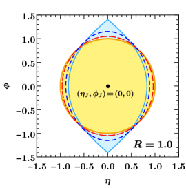
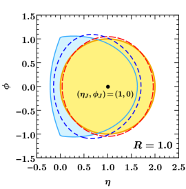
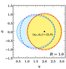
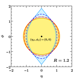
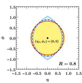
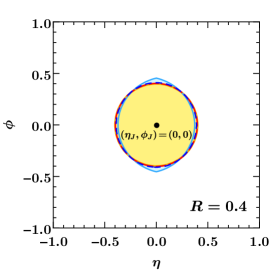
Since these measures only depend on ηisubscript𝜂𝑖\eta_{i} and ϕisubscriptitalic-ϕ𝑖\phi_{i}, we can obtain explicit jet regions in the η𝜂\eta-ϕitalic-ϕ\phi plane. The jet regions for an isolated jet with R=1𝑅1R=1 at different jet rapidities and different R𝑅R at central rapidity are shown in fig. -1379. For small R𝑅R all distance metrics approach a conical partitioning, which means in particular that the deviations from this shape are suppressed by powers of R𝑅R.

Refer to caption
Refer to caption
Refer to caption
Refer to caption
Refer to caption
Refer to caption
Figure -1379: Jet regions (in the limit 𝒯NpTJmuch-less-thansubscript𝒯𝑁superscriptsubscript𝑝𝑇𝐽{\mathcal{T}}_{N}\ll p_{T}^{J}) in the η𝜂\eta-ϕitalic-ϕ\phi-plane for different partitionings for R=1𝑅1R=1 and different ηm=0,1,2subscript𝜂𝑚012\eta_{m}=0,1,2 (top row) and ηm=0subscript𝜂𝑚0\eta_{m}=0 and different R=1.2,0.8,0.4𝑅1.20.80.4R=1.2,0.8,0.4 (bottom row). The conical measure, which is equivalent to anti-kTsubscript𝑘𝑇k_{T}, is shown in yellow, the geometric-R𝑅R measure in light blue, the modified geometric-R𝑅R in blue dashed, and the conical geometric measure (XCone default) in red dashed.

For isolated jets the conical distance measure includes all soft radiation within a distance R𝑅R in η𝜂\eta-ϕitalic-ϕ\phi coordinates from the jet axis into the jet. Thus, in this case the soft partitioning is equivalent to the one obtained in the anti-kTsubscript𝑘𝑇k_{T} algorithm Cacciari:2008gp , which first clusters collinear energetic radiation before clustering soft emissions into the jets (allowing thus for soft-collinear factorization Walsh:2011fz ). As explained above, the algorithm for the jet-axes finding is irrelevant for the description of the soft dynamics and the soft function depends only on the soft partitioning with respect to fixed collinear axes. Thus, the soft function for anti-kTsubscript𝑘𝑇k_{T} jets and N𝑁N-jettiness jets with the conical measure are identical for isolated jets.

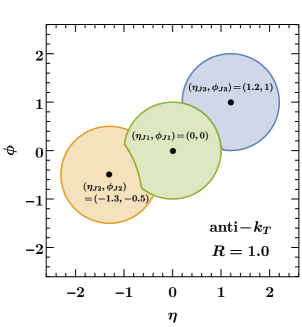
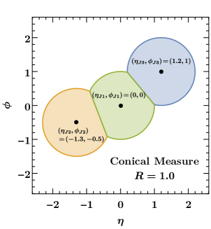
For overlapping jets, the anti-kTsubscript𝑘𝑇k_{T} and N𝑁N-jettiness partitionings differ. The distance metrics in the anti-kTsubscript𝑘𝑇k_{T} algorithm between soft and the clustered collinear radiation depend also on the transverse momenta of the jets, which starts to matter in the singular region 𝒯NpTJmuch-less-thansubscript𝒯𝑁superscriptsubscript𝑝𝑇𝐽{\mathcal{T}}_{N}\ll p_{T}^{J} once two jets start to overlap, i.e. for Rlm<2Rsubscript𝑅𝑙𝑚2𝑅R_{lm}<2R. In this case, anti-kTsubscript𝑘𝑇k_{T} assigns soft radiation in the overlap region to the more energetic jet, while the N𝑁N-jettiness partitioning remains purely geometric. This is illustrated in fig. -1378, for three jets with different transverse momenta that share common jet boundaries. When the distance between two clusters of energetic collinear radiation drops below R𝑅R, anti-kTsubscript𝑘𝑇k_{T} clustering will merge these into a single jet, while the N𝑁N-jettiness partitioning still gives two closeby jets, thus exhibiting a very different behavior.
Refer to caption
Refer to caption
Figure -1378: Partitioning (in the limit 𝒯NpTJmuch-less-thansubscript𝒯𝑁superscriptsubscript𝑝𝑇𝐽{\mathcal{T}}_{N}\ll p_{T}^{J}) for three overlapping jets with pT,1J=2pT,2J=4pT,3Jsubscriptsuperscript𝑝𝐽𝑇12subscriptsuperscript𝑝𝐽𝑇24subscriptsuperscript𝑝𝐽𝑇3p^{J}_{T,1}=2p^{J}_{T,2}=4p^{J}_{T,3} and R=1𝑅1R=1 with distance >Rabsent𝑅>R between their axes. The N𝑁N-jettiness partitioning with the conical distance measure is shown on the left and the anti-kTsubscript𝑘𝑇k_{T} partitioning on the right.

The (modified) geometric-R𝑅R measures in eqs. (14) and (15) have the feature that pTidm(pi)nmpisimilar-tosubscript𝑝𝑇𝑖subscript𝑑𝑚subscript𝑝𝑖subscript𝑛𝑚subscript𝑝𝑖p_{Ti}d_{m}(p_{i})\sim n_{m}\cdot p_{i} is linear in the particle momenta pisubscript𝑝𝑖p_{i}, as for the pure geometric measure in eq. (2) from which they are derived. The geometric-R𝑅R measure was first used in ref. Jouttenus:2013hs to study the jet mass for ppH+1𝑝𝑝𝐻1pp\to H+1 jet, taking advantage of the fact that the soft function for this type of measure was computed in ref. Jouttenus:2011wh . The parameters ρτ(R,ηm)subscript𝜌𝜏𝑅subscript𝜂𝑚\rho_{\tau}(R,\eta_{m}) and ρC(R,ηm)subscript𝜌𝐶𝑅subscript𝜂𝑚\rho_{C}(R,\eta_{m}) are determined by requiring the area in the η𝜂\eta-ϕitalic-ϕ\phi-plane for an isolated jet with rapidity ηmsubscript𝜂𝑚\eta_{m} to be πR2𝜋superscript𝑅2\pi R^{2}, i.e. by solving

ππdϕdηθ[d0(η)dm(ρ,ηm,η,ϕ)]=πR2.superscriptsubscript𝜋𝜋differential-ditalic-ϕsuperscriptsubscriptdifferential-d𝜂𝜃delimited-[]subscript𝑑0𝜂subscript𝑑𝑚𝜌subscript𝜂𝑚𝜂italic-ϕ𝜋superscript𝑅2\int_{-\pi}^{\pi}\!\mathrm{d}\phi\int_{-\infty}^{\infty}\!\!\mathrm{d}\eta\,\theta\bigl{[}d_{0}(\eta)-d_{m}(\rho,\eta_{m},\eta,\phi)\bigr{]}=\pi R^{2}\,. (18)

The solution for ρ𝜌\rho in terms of ηmsubscript𝜂𝑚\eta_{m} and R𝑅R can be computed analytically in an expansion for small R𝑅R, which gives

ρτ(R,ηm)subscript𝜌𝜏𝑅subscript𝜂𝑚\displaystyle\rho_{\tau}(R,\eta_{m}) =R21+tanh|ηm|2{1+2Rπθ(R|ηm|)[1ηm2R2|ηm|RarccosηmR]+𝒪(R2)},absentsuperscript𝑅21subscript𝜂𝑚212𝑅𝜋𝜃𝑅subscript𝜂𝑚delimited-[]1superscriptsubscript𝜂𝑚2superscript𝑅2subscript𝜂𝑚𝑅subscript𝜂𝑚𝑅𝒪superscript𝑅2\displaystyle=R^{2}\frac{1\!+\!\tanh|\eta_{m}|}{2}\biggl{\{}1+\frac{2R}{\pi}\,\theta(R-|\eta_{m}|)\biggl{[}\sqrt{1\!-\!\frac{\eta_{m}^{2}}{R^{2}}}-\frac{|\eta_{m}|}{R}\arccos\frac{\eta_{m}}{R}\biggr{]}\!+\mathcal{O}(R^{2})\biggr{\}},
ρC(R,ηm)subscript𝜌𝐶𝑅subscript𝜂𝑚\displaystyle\rho_{C}(R,\eta_{m}) =R2{1+R24(13tanh2ηm)+𝒪(R4)}.absentsuperscript𝑅21superscript𝑅2413superscript2subscript𝜂𝑚𝒪superscript𝑅4\displaystyle=R^{2}\biggl{\{}1+\frac{R^{2}}{4}\bigl{(}1-3\tanh^{2}\!\eta_{m}\bigr{)}+\mathcal{O}(R^{4})\biggr{\}}\,. (19)

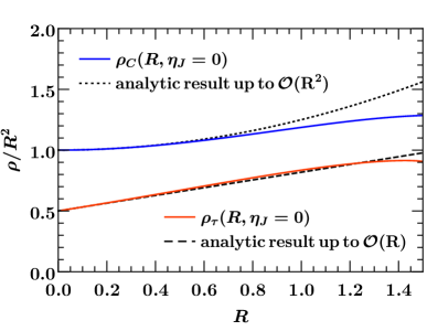
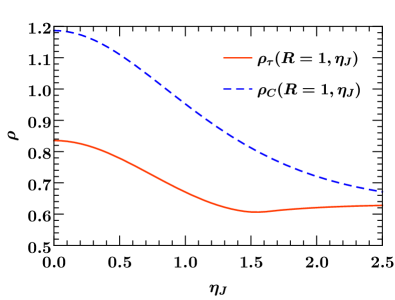
Note that the kink at ηm=0subscript𝜂𝑚0\eta_{m}=0 leads to 𝒪(R)𝒪𝑅\mathcal{O}(R) corrections for ρτsubscript𝜌𝜏\rho_{\tau} for |ηm|<Rsubscript𝜂𝑚𝑅|\eta_{m}|<R. The full R𝑅R dependence is obtained numerically. In fig. -1377, we show ρτsubscript𝜌𝜏\rho_{\tau} and ρCsubscript𝜌𝐶\rho_{C} as functions of R𝑅R for ηm=0subscript𝜂𝑚0\eta_{m}=0 and as functions of ηmsubscript𝜂𝑚\eta_{m} for R=1𝑅1R=1.

Refer to caption
Refer to caption
Figure -1377: Behavior of ρτ(R,ηJ)subscript𝜌𝜏𝑅subscript𝜂𝐽\rho_{\tau}(R,\eta_{J}) and ρC(R,ηJ)subscript𝜌𝐶𝑅subscript𝜂𝐽\rho_{C}(R,\eta_{J}) for the geometric-R𝑅R and modified geometric-R𝑅R measures as functions of R𝑅R at ηJ=0subscript𝜂𝐽0\eta_{J}=0 (left panel) and of ηJsubscript𝜂𝐽\eta_{J} for R=1𝑅1R=1 (right panel).

Compared to the conical measure the shapes of the jet regions are more irregular for the geometric-R𝑅R measures, as seen in fig. -1379. In particular the beam thrust measure in eq. (14) has a cusp at η=0𝜂0\eta=0 due to the absolute value in the beam distance measure, which is not present for the smooth beam C-parameter measure in eq. (15). Furthermore, we also see a distortion from the circular shape for large jet rapidities towards an elongated shape, which is common to both measures since their beam distance measures become identical in the forward region.

Finally, the conical geometric measure was introduced in ref. Stewart:2015waa and corresponds to the XCone default measure. It is designed to combine the linear dependence of pTidm0(pi)subscript𝑝𝑇𝑖subscript𝑑𝑚0subscript𝑝𝑖p_{Ti}d_{m\geq 0}(p_{i}) on the particle momenta of the geometric measures with a nearly conical shape, as can be seen in fig. -1379. One can show that deviations from the circular shape are only of 𝒪(R4)𝒪superscript𝑅4\mathcal{O}(R^{4}) and still independent of the jet rapidity, since the distance measures in eq. (16) only depend on the differences with respect to the jet coordinates. The jet area is πR2𝜋superscript𝑅2\pi R^{2} up to very small corrections of 𝒪(R6)𝒪superscript𝑅6\mathcal{O}(R^{6}), which reach only 1%absentpercent1\approx 1\% even for large R=1.2𝑅1.2R=1.2.

2.3 Factorization for different observable choices

In this section we display the form of the factorized cross section for ppL+N𝑝𝑝𝐿𝑁pp\to L+N jets, where L𝐿L denotes a recoiling color-singlet state, with generic observables in the limit 𝒯NpTJmuch-less-thansubscript𝒯𝑁superscriptsubscript𝑝𝑇𝐽{\mathcal{T}}_{N}\ll p_{T}^{J}. The observables can be categorized according to their parametric behavior close to the jet and beam axes into SCETIsubscriptSCETI{\rm SCET}_{\rm I}-type and SCETIIsubscriptSCETII{\rm SCET}_{\rm II}-type cases. For notational simplicity we assume that the same observable is measured in each jet region (which asymptotically behaves like eq. (11) with ββm1𝛽subscript𝛽𝑚1\beta\equiv\beta_{m\geq 1}). We will mainly focus on the properties of the relevant soft function, which also encodes all dependence of the singular cross section on the distance measure used for the partitioning.

The scaling of the modes in the effective theory follows in general from the constraints on radiation imposed by the N𝑁N-jettiness measurements 𝒯(m)superscript𝒯𝑚{\mathcal{T}}^{(m)} in eq. (8) with m=a,b,1,,N𝑚𝑎𝑏1𝑁m=a,b,1,\dots,N, the jet boundaries determined by the distance measures in eq. (2.3) and potential hierarchies in the hard kinematics. We work in a parametric regime with 𝒯(m)pTJmuch-less-thansuperscript𝒯𝑚superscriptsubscript𝑝𝑇𝐽{\mathcal{T}}^{(m)}\ll p_{T}^{J} and without additional hierarchies in the jet kinematics (which corresponds to a generic SCETSCET{\rm SCET} setup), i.e. assuming hard jets with pT,mJQsimilar-tosuperscriptsubscript𝑝𝑇𝑚𝐽𝑄p_{T,m}^{J}\sim Q, large jet radii R1similar-to𝑅1R\sim 1, well-separated collinear directions nlnm1similar-tosubscript𝑛𝑙subscript𝑛𝑚1n_{l}\cdot n_{m}\sim 1, and nonhierarchical measurements in the different regions 𝒯(l)𝒯(m)similar-tosuperscript𝒯𝑙superscript𝒯𝑚{\mathcal{T}}^{(l)}\sim{\mathcal{T}}^{(m)}. The parametric scaling of the collinear and soft modes is then given by

na,b-collinear:subscript𝑛𝑎𝑏-collinear:\displaystyle n_{a,b}\text{-collinear:} pna,bμsuperscriptsubscript𝑝subscript𝑛𝑎𝑏𝜇\displaystyle p_{n_{a,b}}^{\mu} pTJ(λ4γ,1,λ2γ)na,b,similar-toabsentsuperscriptsubscript𝑝𝑇𝐽subscriptsuperscript𝜆4𝛾1superscript𝜆2𝛾subscript𝑛𝑎𝑏\displaystyle\sim p_{T}^{J}\,(\lambda^{\frac{4}{\gamma}},1,\lambda^{\frac{2}{\gamma}})_{n_{a,b}}\,,
nm1-collinear:subscript𝑛𝑚1-collinear:\displaystyle n_{m\geq 1}\text{-collinear:} pnmμsuperscriptsubscript𝑝subscript𝑛𝑚𝜇\displaystyle\qquad p_{n_{m}}^{\mu} pTJ(λ4β,1,λ2β)nm,similar-toabsentsuperscriptsubscript𝑝𝑇𝐽subscriptsuperscript𝜆4𝛽1superscript𝜆2𝛽subscript𝑛𝑚\displaystyle\sim p_{T}^{J}\,(\lambda^{\frac{4}{\beta}},1,\lambda^{\frac{2}{\beta}})_{n_{m}}\,,
soft: psμsuperscriptsubscript𝑝𝑠𝜇\displaystyle p_{s}^{\mu} pTJ(λ2,λ2,λ2),similar-toabsentsuperscriptsubscript𝑝𝑇𝐽superscript𝜆2superscript𝜆2superscript𝜆2\displaystyle\sim p_{T}^{J}\,(\lambda^{2},\lambda^{2},\lambda^{2})\,, (20)

where we adopt the scaling λ2𝒯N/pTJsimilar-tosuperscript𝜆2subscript𝒯𝑁superscriptsubscript𝑝𝑇𝐽\lambda^{2}\sim\mathcal{T}_{N}/p_{T}^{J}, and give momenta in terms of lightcone coordinates pμ=(np,n¯p,p)nsuperscript𝑝𝜇subscript𝑛𝑝¯𝑛𝑝subscript𝑝perpendicular-to𝑛p^{\mu}=(n\cdot p,\bar{n}\cdot p,p_{\perp})_{n} with respect to the lightcone direction n=(1,n^)𝑛1^𝑛n=(1,\hat{n}) and n¯=(1,n^)¯𝑛1^𝑛\bar{n}=(1,-\hat{n}). The properties of the factorization formulas depend on the values of β𝛽\beta and γ𝛾\gamma and the resulting invariant mass hierarchies between the soft and collinear modes. If β,γ1𝛽𝛾1\beta,\gamma\neq 1 the associated collinear fluctuations live at a different invariant mass scale than the soft modes, leading to a SCETIsubscriptSCETI{\rm SCET}_{\rm I}-type description. Otherwise at least one collinear mode is separated from the soft modes only in rapidity, giving rise to a SCETIIsubscriptSCETII{\rm SCET}_{\rm II}-type theory involving rapidity divergences for the individual bare quantities and a dependence on an associated rapidity RG scale ν𝜈\nu in the renormalized quantities Chiu:2011qc ; Chiu:2012ir . Being fully differential in the hard kinematic phase space ΦNsubscriptΦ𝑁\Phi_{N} and all N𝑁N-jettiness observables 𝒯(m)superscript𝒯𝑚{\mathcal{T}}^{(m)}, the factorization formulae for the four cases with β,γ=1𝛽𝛾1\beta,\gamma=1 and β,γ1𝛽𝛾1\beta,\gamma\neq 1 read:333We do not include effects from Glauber gluon exchange here. For active-parton scattering their perturbative contributions start at 𝒪(αs4)𝒪superscriptsubscript𝛼𝑠4{\cal O}(\alpha_{s}^{4}) Gaunt:2014ska ; Zeng:2015iba and can be calculated and included using the Glauber operator framework of ref. Rothstein:2016bsq . For proton initial states the factorization formulae also do not account for spectator forward scattering effects, since the Glauber Lagrangian of ref. Rothstein:2016bsq has been neglected.

A) γ1𝛾1\gamma\neq 1, β1𝛽1\beta\neq 1 (SCETIsubscriptSCETI{\rm SCET}_{\rm I} beams and SCETIsubscriptSCETI{\rm SCET}_{\rm I} jets): (na,b,1,N𝑛𝑎𝑏1𝑁n\in a,b,1,\dots N)

dσκ(ΦN)d𝒯(a)d𝒯(N)dsubscript𝜎𝜅subscriptΦ𝑁dsuperscript𝒯𝑎dsuperscript𝒯𝑁\displaystyle\frac{\mathrm{d}\sigma_{\kappa}(\Phi_{N})}{\mathrm{d}{\mathcal{T}}^{(a)}\cdots\mathrm{d}{\mathcal{T}}^{(N)}} =(ndkn)tr[H^Nκ(ΦN,μ)S^Nκ({𝒯(m)cmkm},{nm},{dm},μ)]absentsubscriptproduct𝑛dsubscript𝑘𝑛trdelimited-[]superscriptsubscript^𝐻𝑁𝜅subscriptΦ𝑁𝜇superscriptsubscript^𝑆𝑁𝜅superscript𝒯𝑚subscript𝑐𝑚subscript𝑘𝑚subscript𝑛𝑚subscript𝑑𝑚𝜇\displaystyle=\int\Bigl{(}\prod_{n}\mathrm{d}k_{n}\Bigr{)}\,{\rm tr}\Bigl{[}\widehat{H}_{N}^{\kappa}(\Phi_{N},\mu)\,\widehat{S}_{N}^{\kappa}\Bigl{(}\bigl{\{}{\mathcal{T}}^{(m)}-c_{m}k_{m}\bigr{\}},\{n_{m}\},\{d_{m}\},\mu\Bigr{)}\Bigr{]}
×ωaγ1Ba(ωaγ1ka,xa,μ)ωbγ1Bb(ωbγ1kb,xb,μ)j=1Nωjβ1Jj(ωjβ1kj,μ).absentsuperscriptsubscript𝜔𝑎𝛾1subscript𝐵𝑎superscriptsubscript𝜔𝑎𝛾1subscript𝑘𝑎subscript𝑥𝑎𝜇superscriptsubscript𝜔𝑏𝛾1subscript𝐵𝑏superscriptsubscript𝜔𝑏𝛾1subscript𝑘𝑏subscript𝑥𝑏𝜇superscriptsubscriptproduct𝑗1𝑁superscriptsubscript𝜔𝑗𝛽1subscript𝐽𝑗superscriptsubscript𝜔𝑗𝛽1subscript𝑘𝑗𝜇\displaystyle\quad\times\omega_{a}^{\gamma-1}B_{a}\bigl{(}\omega_{a}^{\gamma-1}k_{a},x_{a},\mu\bigr{)}\,\omega_{b}^{\gamma-1}B_{b}\bigl{(}\omega_{b}^{\gamma-1}k_{b},x_{b},\mu\bigr{)}\prod_{j=1}^{N}\omega_{j}^{\beta-1}J_{j}(\omega_{j}^{\beta-1}k_{j},\mu)\,. (21)

B) γ=1𝛾1\gamma=1, β1𝛽1\beta\neq 1 (SCETIIsubscriptSCETII{\rm SCET}_{\rm II} beams and SCETIsubscriptSCETI{\rm SCET}_{\rm I} jets):

dσκ(ΦN)d𝒯(a)d𝒯(N)dsubscript𝜎𝜅subscriptΦ𝑁dsuperscript𝒯𝑎dsuperscript𝒯𝑁\displaystyle\frac{\mathrm{d}\sigma_{\kappa}(\Phi_{N})}{\mathrm{d}{\mathcal{T}}^{(a)}\cdots\mathrm{d}{\mathcal{T}}^{(N)}} =(ndkn)tr[H^Nκ(ΦN,μ)S^Nκ({𝒯(m)cmkm},{nm},{dm},μ,νμ)]absentsubscriptproduct𝑛dsubscript𝑘𝑛trdelimited-[]superscriptsubscript^𝐻𝑁𝜅subscriptΦ𝑁𝜇superscriptsubscript^𝑆𝑁𝜅superscript𝒯𝑚subscript𝑐𝑚subscript𝑘𝑚subscript𝑛𝑚subscript𝑑𝑚𝜇𝜈𝜇\displaystyle=\int\Bigl{(}\prod_{n}\mathrm{d}k_{n}\Bigr{)}\,{\rm tr}\Bigl{[}\widehat{H}_{N}^{\kappa}(\Phi_{N},\mu)\,\widehat{S}_{N}^{\kappa}\Bigl{(}\bigl{\{}{\mathcal{T}}^{(m)}-c_{m}k_{m}\bigr{\}},\{n_{m}\},\{d_{m}\},\mu,\frac{\nu}{\mu}\Bigr{)}\Bigr{]}
×Ba(ka,xa,μ,νωa)Bb(kb,xb,μ,νωb)j=1Nωjβ1Jj(ωjβ1kj,μ).absentsubscript𝐵𝑎subscript𝑘𝑎subscript𝑥𝑎𝜇𝜈subscript𝜔𝑎subscript𝐵𝑏subscript𝑘𝑏subscript𝑥𝑏𝜇𝜈subscript𝜔𝑏superscriptsubscriptproduct𝑗1𝑁superscriptsubscript𝜔𝑗𝛽1subscript𝐽𝑗superscriptsubscript𝜔𝑗𝛽1subscript𝑘𝑗𝜇\displaystyle\quad\times B_{a}\Bigl{(}k_{a},x_{a},\mu,\frac{\nu}{\omega_{a}}\Bigr{)}\,B_{b}\Bigl{(}k_{b},x_{b},\mu,\frac{\nu}{\omega_{b}}\Bigr{)}\prod_{j=1}^{N}\omega_{j}^{\beta-1}J_{j}(\omega_{j}^{\beta-1}k_{j},\mu)\,. (22)

C) γ1𝛾1\gamma\neq 1, β=1𝛽1\beta=1 (SCETIsubscriptSCETI{\rm SCET}_{\rm I} beams and SCETIIsubscriptSCETII{\rm SCET}_{\rm II} jets):

dσκ(ΦN)d𝒯(a)d𝒯(N)dsubscript𝜎𝜅subscriptΦ𝑁dsuperscript𝒯𝑎dsuperscript𝒯𝑁\displaystyle\frac{\mathrm{d}\sigma_{\kappa}(\Phi_{N})}{\mathrm{d}{\mathcal{T}}^{(a)}\cdots\mathrm{d}{\mathcal{T}}^{(N)}} =(ndkn)tr[H^Nκ(ΦN,μ)S^Nκ({𝒯(m)cmkm},{nm},{dm},μ,νμ)]absentsubscriptproduct𝑛dsubscript𝑘𝑛trdelimited-[]superscriptsubscript^𝐻𝑁𝜅subscriptΦ𝑁𝜇superscriptsubscript^𝑆𝑁𝜅superscript𝒯𝑚subscript𝑐𝑚subscript𝑘𝑚subscript𝑛𝑚subscript𝑑𝑚𝜇𝜈𝜇\displaystyle=\int\Bigl{(}\prod_{n}\mathrm{d}k_{n}\Bigr{)}\,{\rm tr}\Bigl{[}\widehat{H}_{N}^{\kappa}(\Phi_{N},\mu)\,\widehat{S}_{N}^{\kappa}\Bigl{(}\bigl{\{}{\mathcal{T}}^{(m)}-c_{m}k_{m}\bigr{\}},\{n_{m}\},\{d_{m}\},\mu,\frac{\nu}{\mu}\Bigr{)}\Bigr{]}
×ωaγ1Ba(ωaγ1ka,xa,μ)ωbγ1Bb(ωbγ1kb,xb,μ)j=1NJj(kj,μ,νωj).absentsuperscriptsubscript𝜔𝑎𝛾1subscript𝐵𝑎superscriptsubscript𝜔𝑎𝛾1subscript𝑘𝑎subscript𝑥𝑎𝜇superscriptsubscript𝜔𝑏𝛾1subscript𝐵𝑏superscriptsubscript𝜔𝑏𝛾1subscript𝑘𝑏subscript𝑥𝑏𝜇superscriptsubscriptproduct𝑗1𝑁subscript𝐽𝑗subscript𝑘𝑗𝜇𝜈subscript𝜔𝑗\displaystyle\quad\times\omega_{a}^{\gamma-1}B_{a}\bigl{(}\omega_{a}^{\gamma-1}k_{a},x_{a},\mu\bigr{)}\,\omega_{b}^{\gamma-1}B_{b}\bigl{(}\omega_{b}^{\gamma-1}k_{b},x_{b},\mu\bigr{)}\prod_{j=1}^{N}J_{j}\Bigl{(}k_{j},\mu,\frac{\nu}{\omega_{j}}\Bigr{)}\,. (23)

D) γ=1𝛾1\gamma=1, β=1𝛽1\beta=1 (SCETIIsubscriptSCETII{\rm SCET}_{\rm II} beams and SCETIIsubscriptSCETII{\rm SCET}_{\rm II} jets):

dσκ(ΦN)d𝒯(a)d𝒯(N)dsubscript𝜎𝜅subscriptΦ𝑁dsuperscript𝒯𝑎dsuperscript𝒯𝑁\displaystyle\frac{\mathrm{d}\sigma_{\kappa}(\Phi_{N})}{\mathrm{d}{\mathcal{T}}^{(a)}\cdots\mathrm{d}{\mathcal{T}}^{(N)}} =(ndkn)tr[H^Nκ(ΦN,μ)S^Nκ({𝒯(m)cmkm},{nm},{dm},μ,νμ)]absentsubscriptproduct𝑛dsubscript𝑘𝑛trdelimited-[]superscriptsubscript^𝐻𝑁𝜅subscriptΦ𝑁𝜇superscriptsubscript^𝑆𝑁𝜅superscript𝒯𝑚subscript𝑐𝑚subscript𝑘𝑚subscript𝑛𝑚subscript𝑑𝑚𝜇𝜈𝜇\displaystyle=\int\Bigl{(}\prod_{n}\mathrm{d}k_{n}\Bigr{)}\,{\rm tr}\Bigl{[}\widehat{H}_{N}^{\kappa}(\Phi_{N},\mu)\,\widehat{S}_{N}^{\kappa}\Bigl{(}\bigl{\{}{\mathcal{T}}^{(m)}-c_{m}k_{m}\bigr{\}},\{n_{m}\},\{d_{m}\},\mu,\frac{\nu}{\mu}\Bigr{)}\Bigr{]}
×Ba(ka,xa,μ,νωa)Bb(kb,xb,μ,νωb)j=1NJj(kj,μ,νωj).absentsubscript𝐵𝑎subscript𝑘𝑎subscript𝑥𝑎𝜇𝜈subscript𝜔𝑎subscript𝐵𝑏subscript𝑘𝑏subscript𝑥𝑏𝜇𝜈subscript𝜔𝑏superscriptsubscriptproduct𝑗1𝑁subscript𝐽𝑗subscript𝑘𝑗𝜇𝜈subscript𝜔𝑗\displaystyle\quad\times B_{a}\Bigl{(}k_{a},x_{a},\mu,\frac{\nu}{\omega_{a}}\Bigr{)}\,B_{b}\Bigl{(}k_{b},x_{b},\mu,\frac{\nu}{\omega_{b}}\Bigr{)}\prod_{j=1}^{N}J_{j}\Bigl{(}k_{j},\mu,\frac{\nu}{\omega_{j}}\Bigr{)}\,. (24)

In eqs. (2.3)–(2.3) the hard function H^Nκsubscriptsuperscript^𝐻𝜅𝑁\widehat{H}^{\kappa}_{N} encodes the hard interaction process for the partonic channel

κa(qa)κb(qb)κ1(q1)κ2(q2)κN(qN)+L(qL),κ={κa,κb;κ1,,κN}formulae-sequencesubscript𝜅𝑎subscript𝑞𝑎subscript𝜅𝑏subscript𝑞𝑏subscript𝜅1subscript𝑞1subscript𝜅2subscript𝑞2subscript𝜅𝑁subscript𝑞𝑁𝐿subscript𝑞𝐿𝜅subscript𝜅𝑎subscript𝜅𝑏subscript𝜅1subscript𝜅𝑁\kappa_{a}(q_{a})\kappa_{b}(q_{b})\to\kappa_{1}(q_{1})\kappa_{2}(q_{2})\dotsb\kappa_{N}(q_{N})+L(q_{L})\,,\qquad\kappa=\{\kappa_{a},\kappa_{b};\kappa_{1},\dots,\kappa_{N}\} (25)

in terms of the massless (label) momenta qmμ=ωmnmμ/2superscriptsubscript𝑞𝑚𝜇subscript𝜔𝑚superscriptsubscript𝑛𝑚𝜇2q_{m}^{\mu}=\omega_{m}n_{m}^{\mu}/2, which satisfy partonic (label) momentum conservation

qaμ+qbμ=q1μ++qNμ+qLμ,superscriptsubscript𝑞𝑎𝜇superscriptsubscript𝑞𝑏𝜇superscriptsubscript𝑞1𝜇superscriptsubscript𝑞𝑁𝜇superscriptsubscript𝑞𝐿𝜇q_{a}^{\mu}+q_{b}^{\mu}=q_{1}^{\mu}+\dotsb+q_{N}^{\mu}+q_{L}^{\mu}\,, (26)

where qLμsuperscriptsubscript𝑞𝐿𝜇q_{L}^{\mu} is the total momentum of the recoiling color-singlet final state. The xa,bsubscript𝑥𝑎𝑏x_{a,b} and label momenta for the initial states are defined via

qa,bμ=ωa,bna,bμ2xa,bEcmna,bμ2.superscriptsubscript𝑞𝑎𝑏𝜇subscript𝜔𝑎𝑏superscriptsubscript𝑛𝑎𝑏𝜇2subscript𝑥𝑎𝑏subscript𝐸cmsuperscriptsubscript𝑛𝑎𝑏𝜇2q_{a,b}^{\mu}=\omega_{a,b}\frac{n_{a,b}^{\mu}}{2}\equiv x_{a,b}E_{\rm cm}\frac{n_{a,b}^{\mu}}{2}\,. (27)

The jet functions Jm1subscript𝐽𝑚1J_{m\geq 1} and beam functions Basubscript𝐵𝑎B_{a}, Bbsubscript𝐵𝑏B_{b} describe the final-state and initial-state collinear dynamics, respectively, and S^Nκsubscriptsuperscript^𝑆𝜅𝑁\widehat{S}^{\kappa}_{N} denotes the soft function. H^Nκsubscriptsuperscript^𝐻𝜅𝑁\widehat{H}^{\kappa}_{N} and S^Nκsubscriptsuperscript^𝑆𝜅𝑁\widehat{S}^{\kappa}_{N} are matrices in color space. The cmsubscript𝑐𝑚c_{m} are the normalization factors of the observable as defined in eq. (11). Due to the requirement 𝒯(m)pTJmuch-less-thansuperscript𝒯𝑚superscriptsubscript𝑝𝑇𝐽{\mathcal{T}}^{(m)}\ll p_{T}^{J} the collinear modes do not resolve the jet boundaries, such that the jet functions are of the inclusive type and have been computed at one-loop in ref. Larkoski:2014uqa for arbitrary values β>0𝛽0\beta>0.444For β=2𝛽2\beta=2 they have been computed before in refs. Bauer:2003pi ; Fleming:2003gt ; Becher:2009th . Note that in the jet functions, for cases C and D (β=1𝛽1\beta=1), a rapidity regularization in close correspondence to refs. Chiu:2011qc ; Chiu:2012ir leads to an additional dependence on the scale ratio ν/ωm𝜈subscript𝜔𝑚\nu/\omega_{m}.

The factorization for the pure SCETIsubscriptSCETI{\rm SCET}_{\rm I} case, for β=γ=2𝛽𝛾2\beta=\gamma=2, is well studied in the literature Stewart:2010tn ; Jouttenus:2011wh and has been applied to phenomenological predictions for single-jet production Jouttenus:2013hs . Also, both cases A and B have been studied in ref. Stewart:2015waa (with the focus on β=2𝛽2\beta=2). In this work, we present for the first time cases C and D, and we will focus on those in the following discussion. These represent a generalization of the previous cases, and assume that the jet and beam axes are insensitive to effects due to mutual recoil or to recoil from soft emissions.

The recoil of the jet axis due to collinear radiation can be relevant for β>1𝛽1\beta>1 (see e.g. ref. Kang:2013nha ), but as discussed in ref. Stewart:2015waa , is avoided by properly aligning the jet axes. For β1𝛽1\beta\leq 1, the jet axis can in addition recoil against soft radiation, leading to nontrivial perpendicular momentum convolutions between the jet, beam, and soft functions for recoil-sensitive axes (see e.g. refs. Dokshitzer:1998kz ; Larkoski:2014uqa ). Recoil-free jet axes avoiding this issue can be defined, e.g., through a global minimization of N𝑁N-jettiness,

𝒯Nsubscript𝒯𝑁\displaystyle{\mathcal{T}}_{N} =minn1,,nNim=a,b,1,,N𝒯(m)(pi)absentsubscriptsubscript𝑛1subscript𝑛𝑁subscript𝑖subscript𝑚𝑎𝑏1𝑁superscript𝒯𝑚subscript𝑝𝑖\displaystyle=\min_{n_{1},\dots,n_{N}}\sum_{i}\sum_{m=a,b,1,\dots,N}{\mathcal{T}}^{(m)}(p_{i})
=minn1,,nNim=a,b,1,,Nfm(ηi,ϕi)pTilmθ(dl(pi)dm(pi)).absentsubscriptsubscript𝑛1subscript𝑛𝑁subscript𝑖subscript𝑚𝑎𝑏1𝑁subscript𝑓𝑚subscript𝜂𝑖subscriptitalic-ϕ𝑖subscript𝑝𝑇𝑖subscriptproduct𝑙𝑚𝜃subscript𝑑𝑙subscript𝑝𝑖subscript𝑑𝑚subscript𝑝𝑖\displaystyle=\min_{n_{1},\dots,n_{N}}\sum_{i}\sum_{m=a,b,1,\dots,N}f_{m}(\eta_{i},\phi_{i})\,p_{Ti}\,\prod_{l\neq m}\theta(d_{l}(p_{i})-d_{m}(p_{i}))\,. (28)

Other sets of axes deviating by only a sufficiently small amount, i.e. by an angle λ2/βmuch-less-thanabsentsuperscript𝜆2𝛽\ll\lambda^{2/\beta}, yield the same result up to power corrections.

The measurement in the beam region requires a separate discussion, as the beam axes are fixed by the collider setup. However, one can still avoid transverse momentum convolutions by making a less granular measurement of the jet energies or transverse momenta, with a procedure analogous to the one discussed in ref. Stewart:2015waa . Momentum conservation in the direction transverse to the beam implies

kTμpT,aμ+pT,bμ=qT,Lμ+m=1NpT,mμ,superscriptsubscript𝑘𝑇𝜇superscriptsubscript𝑝𝑇𝑎𝜇superscriptsubscript𝑝𝑇𝑏𝜇superscriptsubscript𝑞𝑇𝐿𝜇superscriptsubscript𝑚1𝑁superscriptsubscript𝑝𝑇𝑚𝜇\displaystyle k_{T}^{\mu}\equiv p_{T,a}^{\mu}+p_{T,b}^{\mu}=q_{T,L}^{\mu}+\sum_{m=1}^{N}p_{T,m}^{\mu}, (29)

where pT,msubscript𝑝𝑇𝑚p_{T,m} is the transverse component of the m𝑚m-th jet momentum, so that measurements of the jet transverse momenta (or of the pTsubscript𝑝𝑇p_{T} of a recoiling leptonic state) within a bin size ΔpTJpTJλ2/γmuch-greater-thanΔsuperscriptsubscript𝑝𝑇𝐽superscriptsubscript𝑝𝑇𝐽superscript𝜆2𝛾\Delta p_{T}^{J}\gg p_{T}^{J}\lambda^{2/\gamma} for γ>1𝛾1\gamma>1 and ΔpTJpTJλ2much-greater-thanΔsuperscriptsubscript𝑝𝑇𝐽superscriptsubscript𝑝𝑇𝐽superscript𝜆2\Delta p_{T}^{J}\gg p_{T}^{J}\lambda^{2} for γ1𝛾1\gamma\leq 1 allow one to integrate over the unresolved transverse momenta and eliminate residual transverse momentum convolutions. This leads to the appearance of the common beam functions which are known at one-loop for γ=1𝛾1\gamma=1 and γ=2𝛾2\gamma=2 Stewart:2010qs ; Berger:2010xi ; Becher:2010tm ; Becher:2012qa .

The soft function, which we are primarily interested in here, depends on the measurements 𝒯(m)superscript𝒯𝑚{\mathcal{T}}^{(m)} in the different regions, the angles between any collinear directions nlnmsubscript𝑛𝑙subscript𝑛𝑚n_{l}\cdot n_{m}, and the distance measures dmsubscript𝑑𝑚d_{m} involving the jet radius. If either a jet or beam measurement is SCETIIsubscriptSCETII{\rm SCET}_{\rm II} type, it also involves a dependence on the rapidity renormalization scale ν𝜈\nu besides the invariant mass scale μ𝜇\mu. The (bare) soft matrix element is defined as

S^Nκ({km},{nl},{dm})=0|Y^κ({nl})mδ(km𝒯^(m))Y^κ({nl})|0.\displaystyle\widehat{S}^{\kappa}_{N}\bigl{(}\{k_{m}\},\{n_{l}\},\{d_{m}\}\bigr{)}=\Bigl{\langle}0\Bigr{\rvert}\widehat{Y}_{\kappa}^{\dagger}(\{n_{l}\})\prod_{m}\delta(k_{m}-\hat{{\mathcal{T}}}^{(m)})\,\widehat{Y}_{\kappa}(\{n_{l}\})\Bigr{\rvert}0\Bigr{\rangle}\,. (30)

Here 𝒯^(m)superscript^𝒯𝑚\hat{{\mathcal{T}}}^{(m)} denotes the operator that measures 𝒯(m)superscript𝒯𝑚{\mathcal{T}}^{(m)} on all particles in region m𝑚m, i.e.

𝒯^(m)|Xs=iXs𝒯(m)(pi)lmθ[dl(pi)dm(pi)]|Xs.superscript^𝒯𝑚ketsubscript𝑋𝑠subscript𝑖subscript𝑋𝑠superscript𝒯𝑚subscript𝑝𝑖subscriptproduct𝑙𝑚𝜃delimited-[]subscript𝑑𝑙subscript𝑝𝑖subscript𝑑𝑚subscript𝑝𝑖ketsubscript𝑋𝑠\displaystyle\hat{{\mathcal{T}}}^{(m)}|X_{s}\rangle=\sum_{i\in X_{s}}{\mathcal{T}}^{(m)}(p_{i})\prod_{l\neq m}\theta\bigl{[}d_{l}(p_{i})-d_{m}(p_{i})\bigr{]}|X_{s}\rangle\,. (31)

The color matrix Y^κ({nl})subscript^𝑌𝜅subscript𝑛𝑙\widehat{Y}_{\kappa}(\{n_{l}\}) is a product of N+2𝑁2N+2 soft Wilson lines pointing in the collinear directions na,nb,n1,,nNsubscript𝑛𝑎subscript𝑛𝑏subscript𝑛1subscript𝑛𝑁n_{a},n_{b},n_{1},\dots,n_{N}. For a given partonic channel, each of these is given in the color representation of the associated external parton with the appropriate path-ordering prescription. In the following, we use a normalization such that the tree level result for S^Nκsubscriptsuperscript^𝑆𝜅𝑁\widehat{S}^{\kappa}_{N} is diagonal in color space, S^Nκ(0)=𝟏Nmδ(km)subscriptsuperscript^𝑆𝜅0𝑁subscript1𝑁subscriptproduct𝑚𝛿subscript𝑘𝑚\widehat{S}^{\kappa(0)}_{N}={\bf 1}_{N}\prod_{m}\delta(k_{m}).

The full one-loop soft function for processes with at least one final state jet is so far only known for specific cases. In ref. Jouttenus:2011wh it has been computed for the thrust-like N𝑁N-jettiness with β=γ=2𝛽𝛾2\beta=\gamma=2 using them simultaneously for the measurement and partitioning as in eq. (2). In ref. Kasemets:2015uus the one-loop soft function for angularities with β>1𝛽1\beta>1 in e+esuperscript𝑒superscript𝑒e^{+}e^{-} collisions has been calculated also for a common measurement and partitioning. In the following we will extend these calculations to arbitrary angularity measurements (including jet mass) and jet vetoes (including a standard transverse momentum veto) at pp𝑝𝑝pp-colliders with the separate partitionings as described in sec. 2 (including the anti-kTsubscript𝑘𝑇k_{T} case). At one loop, our results with a global measurement in the beam region are identical to those for the corresponding jet-based vetoes.

3 General hemisphere decomposition at one loop
Refer to caption
Refer to caption
Refer to caption
Refer to caption
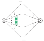
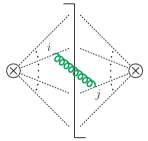
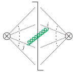
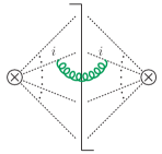
Figure -1376: One loop contributions to the soft function with multiple collinear legs. The vertical line denotes the final-state cut. Diagrams (a) and (b) vanish in Feynman gauge and dimensional regularization, while (c) and (d) lead to eq. (3).

The Feynman diagrams for the computation of the one-loop soft function are displayed in fig. -1376. The virtual diagrams vanish in pure dimensional regularization and the real radiation contribution associated with only one collinear direction vanish in Feynman gauge due to ni2=0superscriptsubscript𝑛𝑖20n_{i}^{2}=0. Thus the one-loop expression is given as a sum over real radiation contributions from different color dipoles each associated with two external hard partons,

S^Nbare(1)({km},{nm},{dm})=i<j𝐓i𝐓jSij({km},{dm})subscriptsuperscript^𝑆bare1𝑁subscript𝑘𝑚subscript𝑛𝑚subscript𝑑𝑚subscript𝑖𝑗subscript𝐓𝑖subscript𝐓𝑗subscript𝑆𝑖𝑗subscript𝑘𝑚subscript𝑑𝑚\displaystyle\widehat{S}^{\mathrm{bare}{(1)}}_{N}(\{k_{m}\},\{n_{m}\},\{d_{m}\})=\sum_{i<j}\mathbf{T}_{i}\cdot\mathbf{T}_{j}\,S_{ij}(\{k_{m}\},\{d_{m}\}) (32)

with i,j=a,b,1,,Nformulae-sequence𝑖𝑗𝑎𝑏1𝑁i,j=a,b,1,\dots,N and

Sij({km},{dm})subscript𝑆𝑖𝑗subscript𝑘𝑚subscript𝑑𝑚\displaystyle S_{ij}(\{k_{m}\},\{d_{m}\}) =2g2(eγEμ24π)ϵddp(2π)d(ν2p0)ηninj(nip)(njp)absent2superscript𝑔2superscriptsuperscript𝑒subscript𝛾𝐸superscript𝜇24𝜋italic-ϵsuperscriptd𝑑𝑝superscript2𝜋𝑑superscript𝜈2subscript𝑝0𝜂subscript𝑛𝑖subscript𝑛𝑗subscript𝑛𝑖𝑝subscript𝑛𝑗𝑝\displaystyle=-2g^{2}\Bigl{(}\frac{e^{\gamma_{E}}\mu^{2}}{4\pi}\Bigr{)}^{\epsilon}\int\!\frac{\mathrm{d}^{d}p}{(2\pi)^{d}}\,\biggl{(}\frac{\nu}{2p_{0}}\biggr{)}^{\eta}\,\frac{n_{i}\cdot n_{j}}{(n_{i}\cdot p)(n_{j}\cdot p)}
×2πδ(p2)θ(p0)F({km},{dm},p).absent2𝜋𝛿superscript𝑝2𝜃superscript𝑝0𝐹subscript𝑘𝑚subscript𝑑𝑚𝑝\displaystyle\quad\times 2\pi\delta(p^{2})\,\theta(p^{0})\,F(\{k_{m}\},\{d_{m}\},p)\,. (33)

We have included a factor to account for the regularization of possible rapidity divergences. Since (ν/(2p0))η(ν/n¯ip)ηsuperscript𝜈2subscript𝑝0𝜂superscript𝜈subscript¯𝑛𝑖𝑝𝜂(\nu/(2p_{0}))^{\eta}\to(\nu/\bar{n}_{i}\cdot p)^{\eta} for pμ(n¯ip)niμ/2superscript𝑝𝜇subscript¯𝑛𝑖𝑝subscriptsuperscript𝑛𝜇𝑖2p^{\mu}\to(\bar{n}_{i}\cdot p)n^{\mu}_{i}/2, the common expressions for the rapidity regularized jet and beam functions can be used. By contrast, naively applying the Wilson line regulator in refs. Chiu:2011qc ; Chiu:2012ir for every single collinear direction would give the factor

(ν|n¯ipnip|)η2×(ν|n¯jpnjp|)η2pμ(n¯ip)niμ2(νn¯ip)η1|n^in^j|η/2.superscript𝜈subscript¯𝑛𝑖𝑝subscript𝑛𝑖𝑝𝜂2superscript𝜈subscript¯𝑛𝑗𝑝subscript𝑛𝑗𝑝𝜂2superscriptsuperscript𝑝𝜇subscript¯𝑛𝑖𝑝subscriptsuperscript𝑛𝜇𝑖2superscript𝜈subscript¯𝑛𝑖𝑝𝜂1superscriptsubscript^𝑛𝑖subscript^𝑛𝑗𝜂2\displaystyle\Bigl{(}\frac{\nu}{|\bar{n}_{i}\cdot p-n_{i}\cdot p|}\Bigr{)}^{\frac{\eta}{2}}\times\Bigl{(}\frac{\nu}{|\bar{n}_{j}\cdot p-n_{j}\cdot p|}\Bigr{)}^{\frac{\eta}{2}}\quad\stackrel{{\scriptstyle p^{\mu}\to(\bar{n}_{i}\cdot p)\frac{n^{\mu}_{i}}{2}}}{{\longrightarrow}}\quad\Bigl{(}\frac{\nu}{\bar{n}_{i}\cdot p}\Bigr{)}^{\eta}\,\frac{1}{|\hat{n}_{i}\cdot\hat{n}_{j}|^{\eta/2}}\,. (34)

The additional factor |n^in^j|η/2superscriptsubscript^𝑛𝑖subscript^𝑛𝑗𝜂2|\hat{n}_{i}\cdot\hat{n}_{j}|^{-\eta/2} leads to different finite 𝒪(η0)𝒪superscript𝜂0\mathcal{O}(\eta^{0}) terms, which would lead to a hard function that differs from the standard MS¯¯MS\overline{\rm MS} result, and hence we chose not to use this regulator here. While refs. Chiu:2011qc ; Chiu:2012ir chose the spatial p3subscript𝑝3p_{3}-component for the regularization, in particular to preserve analyticity properties for virtual corrections, we choose here to only introduce a regulator for real radiation corrections, for which the energy component is suitable.555Rapidity regulators that only act on the real radiation contributions have been used earlier in the literature Becher:2011dz (the regulator we use for our multi-jet situation differs from theirs). An alternative would be a rapidity regulator for the dipole that preserves analyticity and hence can be used for both real and virtual corrections in Sijsubscript𝑆𝑖𝑗S_{ij}, of the form (νninj2|nipnjp|)η.superscript𝜈subscript𝑛𝑖subscript𝑛𝑗2subscript𝑛𝑖𝑝subscript𝑛𝑗𝑝𝜂\displaystyle\Bigl{(}\frac{\nu\,n_{i}\cdot n_{j}}{2|n_{i}\cdot p-n_{j}\cdot p|}\Bigr{)}^{\eta}\,. (35) This regulator does not have an obvious interpretation as coming from the soft Wilson lines. This is related to a moment of the exponential rapidity regulator used in ref. Li:2016axz .

The function F𝐹F incorporates the phase-space constraints on the single soft real emission. In terms of the N𝑁N-jettiness measurements 𝒯(m)(p)superscript𝒯𝑚𝑝{\mathcal{T}}^{(m)}(p) with given distance measures dm(p)subscript𝑑𝑚𝑝d_{m}(p) for m=a,b,1,N𝑚𝑎𝑏1𝑁m=a,b,1,\dots N it reads

F({km},{dm},p)𝐹subscript𝑘𝑚subscript𝑑𝑚𝑝\displaystyle F(\{k_{m}\},\{d_{m}\},p) =mδ(km𝒯(m)(p))lmδ(kl)θ(dl(p)dm(p)).absentsubscript𝑚𝛿subscript𝑘𝑚superscript𝒯𝑚𝑝subscriptproduct𝑙𝑚𝛿subscript𝑘𝑙𝜃subscript𝑑𝑙𝑝subscript𝑑𝑚𝑝\displaystyle=\sum_{m}\delta(k_{m}-{\mathcal{T}}^{(m)}(p))\prod_{l\neq m}\delta(k_{l})\,\theta(d_{l}(p)-d_{m}(p))\,. (36)

To compute the integral in eq. (3) for arbitrary (one-dimensional) measurements and a general phase-space partitioning we generalize the hemisphere decomposition employed in ref. Jouttenus:2011wh . Our method is based on the fact that the full (IR, UV, rapidity) divergent structure of the soft function contribution Sijsubscript𝑆𝑖𝑗S_{ij} is reproduced using arbitrary (IR safe) measurements 𝒯~(i)superscript~𝒯𝑖\tilde{\mathcal{T}}^{(i)}, 𝒯~(j)superscript~𝒯𝑗\tilde{\mathcal{T}}^{(j)} that asymptotically satisfy eq. (11), and using arbitrary distance measures {d~k}subscript~𝑑𝑘\{\tilde{d}_{k}\}, with the only requirement that emissions in the vicinity of the axes nisubscript𝑛𝑖n_{i} and njsubscript𝑛𝑗n_{j} have to be assigned to regions i𝑖i and j𝑗j, respectively. Having found a combination of measures that allows for an analytic calculation one can then compute the mismatch to the correct measurement and phase-space partitioning in terms of finite (numerical) integrals.

The most straightforward choice to enable an analytic calculation with the same singular structure as the full result is to employ directly angularities as measurements in the regions i𝑖i, j𝑗j which are defined by thrust hemispheres, i.e. to use

𝒯~(i)(p)=ci(nip)βi2(n¯ip)1βi2,𝒯~(j)(p)=cj(njp)βj2(n¯jp)1βj2formulae-sequencesuperscript~𝒯𝑖𝑝subscript𝑐𝑖superscriptsubscript𝑛𝑖𝑝subscript𝛽𝑖2superscriptsubscript¯𝑛𝑖𝑝1subscript𝛽𝑖2superscript~𝒯𝑗𝑝subscript𝑐𝑗superscriptsubscript𝑛𝑗𝑝subscript𝛽𝑗2superscriptsubscript¯𝑛𝑗𝑝1subscript𝛽𝑗2\displaystyle\tilde{\mathcal{T}}^{(i)}(p)=c_{i}\,(n_{i}\cdot p)^{\frac{\beta_{i}}{2}}(\bar{n}_{i}\cdot p)^{1-\frac{\beta_{i}}{2}}\,,\quad\tilde{\mathcal{T}}^{(j)}(p)=c_{j}(n_{j}\cdot p)^{\frac{\beta_{j}}{2}}(\bar{n}_{j}\cdot p)^{1-\frac{\beta_{j}}{2}}\, (37)

with the distance measures

d~i(p)=nipρi,d~j(p)=njpρj,d~ki,j(p)=.formulae-sequencesubscript~𝑑𝑖𝑝subscript𝑛𝑖𝑝subscript𝜌𝑖formulae-sequencesubscript~𝑑𝑗𝑝subscript𝑛𝑗𝑝subscript𝜌𝑗subscript~𝑑𝑘𝑖𝑗𝑝\displaystyle\tilde{d}_{i}(p)=\frac{n_{i}\cdot p}{\rho_{i}}\,,\qquad\tilde{d}_{j}(p)=\frac{n_{j}\cdot p}{\rho_{j}}\,,\qquad\tilde{d}_{k\neq i,j}(p)=\infty\,. (38)

We have included factors ρi,ρjsubscript𝜌𝑖subscript𝜌𝑗\rho_{i},\rho_{j} to allow for the possibility of nonequal hemisphere regions i𝑖i and j𝑗j, which we will exploit in sec. 4 to analytically calculate the result in the small-R𝑅R limit. Taking into account the difference to the actual jet boundaries and measurement, we decompose the measurement function F𝐹F for the dipole correction Sijsubscript𝑆𝑖𝑗S_{ij} as

F({kl},{dl},p)𝐹subscript𝑘𝑙subscript𝑑𝑙𝑝\displaystyle F(\{k_{l}\},\{d_{l}\},p) =F~i<j({kl},p)+ΔFi<j({kl},p)+F~j<i({kl},p)+ΔFj<i({kl},p)absentsubscript~𝐹𝑖𝑗subscript𝑘𝑙𝑝Δsubscript𝐹𝑖𝑗subscript𝑘𝑙𝑝subscript~𝐹𝑗𝑖subscript𝑘𝑙𝑝Δsubscript𝐹𝑗𝑖subscript𝑘𝑙𝑝\displaystyle=\tilde{F}_{i<j}(\{k_{l}\},p)+\Delta F_{i<j}(\{k_{l}\},p)+\tilde{F}_{j<i}(\{k_{l}\},p)+\Delta F_{j<i}(\{k_{l}\},p)
+m=a,b,1,,NFijm({kl},{dl},p),subscript𝑚𝑎𝑏1𝑁superscriptsubscript𝐹𝑖𝑗𝑚subscript𝑘𝑙subscript𝑑𝑙𝑝\displaystyle\quad+\sum_{m=a,b,1,\dots,N}F_{ij}^{m}(\{k_{l}\},\{d_{l}\},p)\,, (39)

with all indices distinguishing separate beam regions a,b𝑎𝑏a,b and

F~i<j({kl},p)subscript~𝐹𝑖𝑗subscript𝑘𝑙𝑝\displaystyle\tilde{F}_{i<j}(\{k_{l}\},p) =δ(ki𝒯~(i)(p))θ(njpρjnipρi)liδ(kl),absent𝛿subscript𝑘𝑖superscript~𝒯𝑖𝑝𝜃subscript𝑛𝑗𝑝subscript𝜌𝑗subscript𝑛𝑖𝑝subscript𝜌𝑖subscriptproduct𝑙𝑖𝛿subscript𝑘𝑙\displaystyle=\delta\bigl{(}k_{i}-\tilde{{\mathcal{T}}}^{(i)}(p)\bigr{)}\,\theta\Bigl{(}\frac{n_{j}\cdot p}{\rho_{j}}-\frac{n_{i}\cdot p}{\rho_{i}}\Bigr{)}\,\prod_{l\neq i}\delta(k_{l})\,,
ΔFi<j({kl},p)Δsubscript𝐹𝑖𝑗subscript𝑘𝑙𝑝\displaystyle\Delta F_{i<j}(\{k_{l}\},p) =[δ(ki𝒯(i)(p))δ(ki𝒯~(i)(p))]θ(njpρjnipρi)liδ(kl),absentdelimited-[]𝛿subscript𝑘𝑖superscript𝒯𝑖𝑝𝛿subscript𝑘𝑖superscript~𝒯𝑖𝑝𝜃subscript𝑛𝑗𝑝subscript𝜌𝑗subscript𝑛𝑖𝑝subscript𝜌𝑖subscriptproduct𝑙𝑖𝛿subscript𝑘𝑙\displaystyle=\Bigl{[}\delta\bigl{(}k_{i}-{\mathcal{T}}^{(i)}(p)\bigr{)}-\delta\bigl{(}k_{i}-\tilde{{\mathcal{T}}}^{(i)}(p)\bigr{)}\Bigr{]}\,\theta\Bigl{(}\frac{n_{j}\cdot p}{\rho_{j}}-\frac{n_{i}\cdot p}{\rho_{i}}\Bigr{)}\,\prod_{l\neq i}\delta(k_{l})\,,
Fiji({kl},{dn},p)superscriptsubscript𝐹𝑖𝑗𝑖subscript𝑘𝑙subscript𝑑𝑛𝑝\displaystyle F_{ij}^{i}(\{k_{l}\},\{d_{n}\},p) =[δ(ki𝒯(i)(p))δ(kj)δ(kj𝒯(j)(p))δ(ki)]absentdelimited-[]𝛿subscript𝑘𝑖superscript𝒯𝑖𝑝𝛿subscript𝑘𝑗𝛿subscript𝑘𝑗superscript𝒯𝑗𝑝𝛿subscript𝑘𝑖\displaystyle=\Bigl{[}\delta\bigl{(}k_{i}-{\mathcal{T}}^{(i)}(p)\bigr{)}\,\delta(k_{j})-\delta\bigl{(}k_{j}-{\mathcal{T}}^{(j)}(p)\bigr{)}\,\delta(k_{i})\Bigr{]}
×θ(nipρinjpρj)θ(dj(p)di(p))li,jθ(dl(p)di(p))δ(kl),absent𝜃subscript𝑛𝑖𝑝subscript𝜌𝑖subscript𝑛𝑗𝑝subscript𝜌𝑗𝜃subscript𝑑𝑗𝑝subscript𝑑𝑖𝑝subscriptproduct𝑙𝑖𝑗𝜃subscript𝑑𝑙𝑝subscript𝑑𝑖𝑝𝛿subscript𝑘𝑙\displaystyle\quad\times\theta\Bigl{(}\frac{n_{i}\cdot p}{\rho_{i}}-\frac{n_{j}\cdot p}{\rho_{j}}\Bigr{)}\,\theta\bigl{(}d_{j}(p)-d_{i}(p)\bigr{)}\prod_{l\neq i,j}\theta\bigl{(}d_{l}(p)-d_{i}(p)\bigr{)}\,\delta(k_{l})\,,
Fijmi,j({kl},{dn},p)superscriptsubscript𝐹𝑖𝑗𝑚𝑖𝑗subscript𝑘𝑙subscript𝑑𝑛𝑝\displaystyle F_{ij}^{m\neq i,j}(\{k_{l}\},\{d_{n}\},p) =[δ(km𝒯(m)(p))δ(ki)δ(ki𝒯(i)(p))δ(km)]absentdelimited-[]𝛿subscript𝑘𝑚superscript𝒯𝑚𝑝𝛿subscript𝑘𝑖𝛿subscript𝑘𝑖superscript𝒯𝑖𝑝𝛿subscript𝑘𝑚\displaystyle=\Bigl{[}\delta\bigl{(}k_{m}-{\mathcal{T}}^{(m)}(p)\bigr{)}\,\delta(k_{i})-\delta\bigl{(}k_{i}-{\mathcal{T}}^{(i)}(p)\bigr{)}\,\delta(k_{m})\Bigr{]}
×θ(njpρjnipρi)θ(di(p)dm(p))liθ(dl(p)dm(p))δ(kl)absent𝜃subscript𝑛𝑗𝑝subscript𝜌𝑗subscript𝑛𝑖𝑝subscript𝜌𝑖𝜃subscript𝑑𝑖𝑝subscript𝑑𝑚𝑝subscriptproduct𝑙𝑖𝜃subscript𝑑𝑙𝑝subscript𝑑𝑚𝑝𝛿subscript𝑘𝑙\displaystyle\quad\times\theta\Bigl{(}\frac{n_{j}\cdot p}{\rho_{j}}-\frac{n_{i}\cdot p}{\rho_{i}}\Bigr{)}\,\theta\bigl{(}d_{i}(p)-d_{m}(p)\bigr{)}\prod_{l\neq i}\theta\bigl{(}d_{l}(p)-d_{m}(p)\bigr{)}\,\delta(k_{l})
+(ij).\displaystyle\quad+(i\leftrightarrow j)\,. (40)

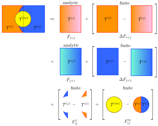
The terms F~j<isubscript~𝐹𝑗𝑖\tilde{F}_{j<i}, ΔFj<iΔsubscript𝐹𝑗𝑖\Delta F_{j<i}, and Fijjsubscriptsuperscript𝐹𝑗𝑖𝑗F^{j}_{ij} in eq. (3) are defined in analogy by replacing ij𝑖𝑗i\leftrightarrow j in these expressions for F~i<jsubscript~𝐹𝑖𝑗\tilde{F}_{i<j}, ΔFi<jΔsubscript𝐹𝑖𝑗\Delta F_{i<j} and Fijisubscriptsuperscript𝐹𝑖𝑖𝑗F^{i}_{ij}. A specific example for this hemisphere decomposition is illustrated in fig. -1375.

The F~i<jsubscript~𝐹𝑖𝑗\tilde{F}_{i<j} denote the measurement of 𝒯~(i)superscript~𝒯𝑖\tilde{\mathcal{T}}^{(i)} in the hemisphere i𝑖i, which can be computed analytically and encodes all divergences. The measurement contribution ΔFi<jΔsubscript𝐹𝑖𝑗\Delta F_{i<j} is present if 𝒯(i)superscript𝒯𝑖{\mathcal{T}}^{(i)} is not identical to the angularity 𝒯~(i)superscript~𝒯𝑖\tilde{\mathcal{T}}^{(i)}. It corrects for this mismatch within the hemisphere boundaries and therefore does not depend on the final partitioning. Since 𝒯(i)superscript𝒯𝑖{\mathcal{T}}^{(i)} and 𝒯~(i)superscript~𝒯𝑖\tilde{\mathcal{T}}^{(i)} yield the same collinear and rapidity divergences and also the soft divergences cancel in the difference of the two IR-safe observables this is a finite correction. The remaining pieces Fijksubscriptsuperscript𝐹𝑘𝑖𝑗F^{k}_{ij} correct the measurement with the hemisphere boundaries to the actual partitioning given in terms of the distance measures {dh}subscript𝑑\{d_{h}\}. Here the superscript m𝑚m indicates that the measurement of 𝒯(m)superscript𝒯𝑚{\mathcal{T}}^{(m)} instead of 𝒯(i)superscript𝒯𝑖{\mathcal{T}}^{(i)} or 𝒯(j)superscript𝒯𝑗{\mathcal{T}}^{(j)} needs to be performed in the associated phase space region where dmsubscript𝑑𝑚d_{m} is minimal. For m=i𝑚𝑖m=i and m=j𝑚𝑗m=j this corresponds to the boundary mismatch corrections between the regions i𝑖i and j𝑗j. The only singularities in the phase space mismatch regions are soft IR divergences which cancel between two IR safe measurements, such that the corresponding correction to the soft function is also finite and can be calculated numerically in terms of finite (observable and partitioning dependent) integrals.
Refer to caption
Figure -1375: Illustration of the hemisphere decomposition of the measurement function in eq. (3) into analytic contributions containing all divergent corrections. The remaining finite corrections accounting for the mismatch in measurement or partitioning can be computed by numerical integrations. The color of the filling indicates which variable is measured. For simplicity we illustrate a case where the correction Fijisuperscriptsubscript𝐹𝑖𝑗𝑖F_{ij}^{i} vanishes.

We decompose the contribution of the ij𝑖𝑗ij dipole to the soft function in direct correspondence with eq. (3)

Sij({kl},{nk},{dm})subscript𝑆𝑖𝑗subscript𝑘𝑙subscript𝑛𝑘subscript𝑑𝑚\displaystyle S_{ij}(\{k_{l}\},\{n_{k}\},\{d_{m}\}) =S~i<j({kl},s^ij)+ΔSi<j({kl},s^ij)+S~j<i({kl},s^ij)+ΔSj<i({kl},s^ij)absentsubscript~𝑆𝑖𝑗subscript𝑘𝑙subscript^𝑠𝑖𝑗Δsubscript𝑆𝑖𝑗subscript𝑘𝑙subscript^𝑠𝑖𝑗subscript~𝑆𝑗𝑖subscript𝑘𝑙subscript^𝑠𝑖𝑗Δsubscript𝑆𝑗𝑖subscript𝑘𝑙subscript^𝑠𝑖𝑗\displaystyle=\tilde{S}_{i<j}(\{k_{l}\},\hat{s}_{ij})+\Delta S_{i<j}(\{k_{l}\},\hat{s}_{ij})+\tilde{S}_{j<i}(\{k_{l}\},\hat{s}_{ij})+\Delta S_{j<i}(\{k_{l}\},\hat{s}_{ij})
+m=a,b,1,,NSijm({kl},{dn},s^ij),subscript𝑚𝑎𝑏1𝑁superscriptsubscript𝑆𝑖𝑗𝑚subscript𝑘𝑙subscript𝑑𝑛subscript^𝑠𝑖𝑗\displaystyle\quad+\sum_{m=a,b,1,\dots,N}S_{ij}^{m}(\{k_{l}\},\{d_{n}\},\hat{s}_{ij})\,, (41)

where the terms on the right-hand side distinguish between two beam regions with separate measurements.

The expressions for the individual terms follow by replacing the measurement F({kl},{dn},p)𝐹subscript𝑘𝑙subscript𝑑𝑛𝑝F(\{k_{l}\},\{d_{n}\},p) in eq. (32) by the corresponding term in eq. (3). The hemisphere corrections to the soft function S~i<jsubscript~𝑆𝑖𝑗\tilde{S}_{i<j} and S~j<isubscript~𝑆𝑗𝑖\tilde{S}_{j<i} have been calculated analytically for βi=2subscript𝛽𝑖2\beta_{i}=2 in Jouttenus:2011wh . For βi1subscript𝛽𝑖1\beta_{i}\neq 1 the result has been given in ref. Kasemets:2015uus in terms of a finite numerical integral. The latter can be evaluated analytically and vanishes for ρi=ρjsubscript𝜌𝑖subscript𝜌𝑗\rho_{i}=\rho_{j}. This yields the bare result

S~i<jβi1({kl},s^ij)superscriptsubscript~𝑆𝑖𝑗subscript𝛽𝑖1subscript𝑘𝑙subscript^𝑠𝑖𝑗\displaystyle\tilde{S}_{i<j}^{\beta_{i}\neq 1}(\{k_{l}\},\hat{s}_{ij}) =αs4π1βi1liδ(kl){8μξi<j1(kiμξi<j)4ϵ1μξi<j0(kiμξi<j)\displaystyle=\frac{\alpha_{s}}{4\pi}\frac{1}{\beta_{i}-1}\,\prod_{l\neq i}\delta(k_{l})\,\biggl{\{}\frac{8}{\mu\,\xi_{i<j}}\,\mathcal{L}_{1}\biggl{(}\frac{k_{i}}{\mu\,\xi_{i<j}}\biggr{)}-\frac{4}{\epsilon}\frac{1}{\mu\,\xi_{i<j}}\,\mathcal{L}_{0}\biggl{(}\frac{k_{i}}{\mu\,\xi_{i<j}}\biggr{)} (42)
+δ(ki)[2ϵ2π26(βi2)(βi1)θ(ρiρjs^i¯j1)ln2(ρiρjs^i¯j)]+𝒪(ϵ)},\displaystyle\quad+\delta(k_{i})\biggl{[}\frac{2}{\epsilon^{2}}-\frac{\pi^{2}}{6}-(\beta_{i}-2)(\beta_{i}-1)\,\theta\Bigl{(}\frac{\rho_{i}}{\rho_{j}}\hat{s}_{\bar{i}j}-1\Bigr{)}\ln^{2}\Bigl{(}\frac{\rho_{i}}{\rho_{j}}\hat{s}_{\bar{i}j}\Bigr{)}\biggr{]}+\mathcal{O}(\epsilon)\biggr{\}}\,,

with the rescaling factor ξi<jsubscript𝜉𝑖𝑗\xi_{i<j} given in terms of the angular term s^ijsubscript^𝑠𝑖𝑗\hat{s}_{ij}, with

ξi<jci(ρiρjs^ij)βi12,s^ijninj2=1cosθij2,s^i¯jn¯inj2=1+cosθij2.formulae-sequenceformulae-sequencesubscript𝜉𝑖𝑗subscript𝑐𝑖superscriptsubscript𝜌𝑖subscript𝜌𝑗subscript^𝑠𝑖𝑗subscript𝛽𝑖12subscript^𝑠𝑖𝑗subscript𝑛𝑖subscript𝑛𝑗21subscript𝜃𝑖𝑗2subscript^𝑠¯𝑖𝑗subscript¯𝑛𝑖subscript𝑛𝑗21subscript𝜃𝑖𝑗2\displaystyle\xi_{i<j}\equiv c_{i}\Bigl{(}\frac{\rho_{i}}{\rho_{j}}\hat{s}_{ij}\Bigr{)}^{\frac{\beta_{i}-1}{2}}\,,\quad\hat{s}_{ij}\equiv\frac{n_{i}\cdot n_{j}}{2}=\frac{1-\cos\theta_{ij}}{2}\,,\quad\hat{s}_{\bar{i}j}\equiv\frac{\bar{n}_{i}\cdot n_{j}}{2}=\frac{1+\cos\theta_{ij}}{2}\,. (43)

The plus distributions nsubscript𝑛{\mathcal{L}}_{n} are defined as

n(y)[θ(y)lnnyy]+.subscript𝑛𝑦subscriptdelimited-[]𝜃𝑦superscript𝑛𝑦𝑦\displaystyle{\mathcal{L}}_{n}(y)\equiv\bigg{[}\frac{\theta(y)\ln^{n}y}{y}\bigg{]}_{+}\,. (44)

For βi=1subscript𝛽𝑖1\beta_{i}=1 the computation is carried out in app. A which gives the result

S~i<jβi=1({kl},s^ij)superscriptsubscript~𝑆𝑖𝑗subscript𝛽𝑖1subscript𝑘𝑙subscript^𝑠𝑖𝑗\displaystyle\tilde{S}_{i<j}^{\beta_{i}=1}(\{k_{l}\},\hat{s}_{ij}) =αs4πliδ(kl){8μci1(kiμci)8μci0(kiμci)[1η+ln(νμρiρjs^ij)]\displaystyle=\frac{\alpha_{s}}{4\pi}\,\prod_{l\neq i}\delta(k_{l})\,\biggl{\{}\frac{8}{\mu\,c_{i}}\,\mathcal{L}_{1}\biggl{(}\frac{k_{i}}{\mu\,c_{i}}\biggr{)}-\frac{8}{\mu\,c_{i}}\,\mathcal{L}_{0}\biggl{(}\frac{k_{i}}{\mu\,c_{i}}\biggr{)}\biggl{[}\frac{1}{\eta}+\ln\biggl{(}\frac{\nu}{\mu}\sqrt{\frac{\rho_{i}}{\rho_{j}}\hat{s}_{ij}}\biggl{)}\biggr{]}
+δ(ki)[4ηϵ2ϵ2+4ϵln(νμρiρjs^ij)+π26+θ(ρiρjs^i¯j1)ln2(ρiρjs^i¯j)]𝛿subscript𝑘𝑖delimited-[]4𝜂italic-ϵ2superscriptitalic-ϵ24italic-ϵ𝜈𝜇subscript𝜌𝑖subscript𝜌𝑗subscript^𝑠𝑖𝑗superscript𝜋26𝜃subscript𝜌𝑖subscript𝜌𝑗subscript^𝑠¯𝑖𝑗1superscript2subscript𝜌𝑖subscript𝜌𝑗subscript^𝑠¯𝑖𝑗\displaystyle\quad+\delta(k_{i})\biggl{[}\frac{4}{\eta\,\epsilon}-\frac{2}{\epsilon^{2}}+\frac{4}{\epsilon}\,\ln\biggl{(}\frac{\nu}{\mu}\sqrt{\frac{\rho_{i}}{\rho_{j}}\hat{s}_{ij}}\biggr{)}+\frac{\pi^{2}}{6}+\theta\Bigl{(}\frac{\rho_{i}}{\rho_{j}}\hat{s}_{\bar{i}j}-1\Bigr{)}\ln^{2}\Bigl{(}\frac{\rho_{i}}{\rho_{j}}\hat{s}_{\bar{i}j}\Bigr{)}\biggr{]}
+𝒪(η,ϵ)}.\displaystyle\quad+\mathcal{O}(\eta,\epsilon)\biggr{\}}\,. (45)

The hemisphere results S~j<isubscript~𝑆𝑗𝑖\tilde{S}_{j<i} are given by simply replacing ij𝑖𝑗i\leftrightarrow j in eqs. (42) and (3).

We will now explicitly display the corrections to the hemisphere results in eqs. (42) and (3) in terms of finite integrals that can be computed numerically. Depending on the specific partitioning and N𝑁N-jettiness measurement, different integration variables can be appropriate, e.g. the rapidity η𝜂\eta and azimuthal angle ϕitalic-ϕ\phi in the lab frame (i.e. coordinates with respect to the beam axis) or the relative rapidity ηsuperscript𝜂\eta^{\prime} and azimuthal angle ϕsuperscriptitalic-ϕ\phi^{\prime} in a boosted frame where the collinear directions nisubscript𝑛𝑖n_{i} and njsubscript𝑛𝑗n_{j} are back-to-back. The former is usually more convenient for the conical (anti-kTsubscript𝑘𝑇k_{T}) distance measure in eq. (13) since the integration boundaries are just circles in the η𝜂\eta-ϕitalic-ϕ\phi plane, while the geometric measures in eqs. (14)–(16) involve naturally the momentum projections nipsubscript𝑛𝑖𝑝n_{i}\cdot p, njpsubscript𝑛𝑗𝑝n_{j}\cdot p for which the variables ηsuperscript𝜂\eta^{\prime}, ϕsuperscriptitalic-ϕ\phi^{\prime} are usually more practical (see refs. Jouttenus:2011wh ; Kasemets:2015uus ). For definiteness we use here beam coordinates, since our general N𝑁N-jettiness measurements for ppN𝑝𝑝𝑁pp\to N jets in eq. (8) and also the distance measures in eqs. (13)–(16) are displayed in terms of those, and since our main focus will be the anti-kTsubscript𝑘𝑇k_{T} case. First we write the momentum projections in eqs. (3), (37) and (38) as

nkp=pTgk(η,ϕ),n¯kp=pTgk¯(η,ϕ)formulae-sequencesubscript𝑛𝑘𝑝subscript𝑝𝑇subscript𝑔𝑘𝜂italic-ϕsubscript¯𝑛𝑘𝑝subscript𝑝𝑇subscript𝑔¯𝑘𝜂italic-ϕ\displaystyle n_{k}\cdot p=p_{T}\,g_{k}(\eta,\phi)\,,\qquad\bar{n}_{k}\cdot p=p_{T}\,g_{\bar{k}}(\eta,\phi) (46)

with

ga(η,ϕ)subscript𝑔𝑎𝜂italic-ϕ\displaystyle g_{a}(\eta,\phi) g0(η,ϕ)=eη,absentsubscript𝑔0𝜂italic-ϕsuperscript𝑒𝜂\displaystyle\equiv g_{0}(\eta,\phi)=e^{-\eta}\,,
gb(η,ϕ)subscript𝑔𝑏𝜂italic-ϕ\displaystyle g_{b}(\eta,\phi) g0¯(η,ϕ)=eη,absentsubscript𝑔¯0𝜂italic-ϕsuperscript𝑒𝜂\displaystyle\equiv g_{\bar{0}}(\eta,\phi)=e^{\eta}\,,
gm>0(η,ϕ)subscript𝑔𝑚0𝜂italic-ϕ\displaystyle g_{m>0}(\eta,\phi) =cosh(ηηm)cos(ϕϕm)coshηm,absent𝜂subscript𝜂𝑚italic-ϕsubscriptitalic-ϕ𝑚subscript𝜂𝑚\displaystyle=\frac{\cosh(\eta-\eta_{m})-\cos(\phi-\phi_{m})}{\cosh\eta_{m}}\,,
gm¯>0(η,ϕ)subscript𝑔¯𝑚0𝜂italic-ϕ\displaystyle g_{\bar{m}>0}(\eta,\phi) =cosh(η+ηm)+cos(ϕϕm)coshηm.absent𝜂subscript𝜂𝑚italic-ϕsubscriptitalic-ϕ𝑚subscript𝜂𝑚\displaystyle=\frac{\cosh(\eta+\eta_{m})+\cos(\phi-\phi_{m})}{\cosh\eta_{m}}\,. (47)

Keeping only the ϵitalic-ϵ\epsilon-dependence in the phase space integration of eq. (3) which is required to regulate the soft singularities, we can write the correction terms as

ΔSi<j({kl},s^ij)Δsubscript𝑆𝑖𝑗subscript𝑘𝑙subscript^𝑠𝑖𝑗\displaystyle\Delta S_{i<j}(\{k_{l}\},\hat{s}_{ij}) =αsπ2μ2ϵ0dpTpT1+2ϵππdϕdηs^ijgi(η,ϕ)gj(η,ϕ)ΔFi<j({kl},p)+𝒪(ϵ),absentsubscript𝛼𝑠superscript𝜋2superscript𝜇2italic-ϵsuperscriptsubscript0dsubscript𝑝𝑇superscriptsubscript𝑝𝑇12italic-ϵsuperscriptsubscript𝜋𝜋differential-ditalic-ϕsuperscriptsubscriptdifferential-d𝜂subscript^𝑠𝑖𝑗subscript𝑔𝑖𝜂italic-ϕsubscript𝑔𝑗𝜂italic-ϕΔsubscript𝐹𝑖𝑗subscript𝑘𝑙𝑝𝒪italic-ϵ\displaystyle=-\frac{\alpha_{s}}{\pi^{2}}\,\mu^{2\epsilon}\int_{0}^{\infty}\frac{\mathrm{d}p_{T}}{p_{T}^{1+2\epsilon}}\int_{-\pi}^{\pi}\mathrm{d}\phi\int_{-\infty}^{\infty}\mathrm{d}\eta\,\frac{\hat{s}_{ij}}{g_{i}(\eta,\phi)\,g_{j}(\eta,\phi)}\,\Delta F_{i<j}(\{k_{l}\},p)+\mathcal{O}(\epsilon)\,, (48)

and similarly for Sijmsubscriptsuperscript𝑆𝑚𝑖𝑗S^{m}_{ij}. We can then use that

μ2ϵ0dpTpT1+2ϵ[δ(ki)δ(kmpTfm(η,ϕ))δ(kipTfi(η,ϕ))δ(km)]superscript𝜇2italic-ϵsuperscriptsubscript0dsubscript𝑝𝑇superscriptsubscript𝑝𝑇12italic-ϵdelimited-[]𝛿subscript𝑘𝑖𝛿subscript𝑘𝑚subscript𝑝𝑇subscript𝑓𝑚𝜂italic-ϕ𝛿subscript𝑘𝑖subscript𝑝𝑇subscript𝑓𝑖𝜂italic-ϕ𝛿subscript𝑘𝑚\displaystyle\mu^{2\epsilon}\int_{0}^{\infty}\frac{\mathrm{d}p_{T}}{p_{T}^{1+2\epsilon}}\bigl{[}\delta(k_{i})\,\delta\bigl{(}k_{m}-p_{T}f_{m}(\eta,\phi)\bigr{)}-\delta\bigl{(}k_{i}-p_{T}f_{i}(\eta,\phi)\bigr{)}\,\delta(k_{m})\bigr{]}
=δ(ki)1μ0(kmμ)1μ0(kiμ)δ(km)ln(fm(η,ϕ)fi(η,ϕ))δ(ki)δ(km)+𝒪(ϵ).absent𝛿subscript𝑘𝑖1𝜇subscript0subscript𝑘𝑚𝜇1𝜇subscript0subscript𝑘𝑖𝜇𝛿subscript𝑘𝑚subscript𝑓𝑚𝜂italic-ϕsubscript𝑓𝑖𝜂italic-ϕ𝛿subscript𝑘𝑖𝛿subscript𝑘𝑚𝒪italic-ϵ\displaystyle\qquad=\delta(k_{i})\,\frac{1}{\mu}{\mathcal{L}}_{0}\Bigl{(}\frac{k_{m}}{\mu}\Bigr{)}-\frac{1}{\mu}\,{\mathcal{L}}_{0}\Bigl{(}\frac{k_{i}}{\mu}\Bigr{)}\,\delta(k_{m})-\ln\biggl{(}\frac{f_{m}(\eta,\phi)}{f_{i}(\eta,\phi)}\biggr{)}\,\delta(k_{i})\,\delta(k_{m})+\mathcal{O}(\epsilon)\,. (49)

To obtain the correction ΔSi<jΔsubscript𝑆𝑖𝑗\Delta S_{i<j} we replace in eq. (3) kmkisubscript𝑘𝑚subscript𝑘𝑖k_{m}\to k_{i}, fmf~i=cigiβi/2gi¯1βi/2subscript𝑓𝑚subscript~𝑓𝑖subscript𝑐𝑖subscriptsuperscript𝑔subscript𝛽𝑖2𝑖subscriptsuperscript𝑔1subscript𝛽𝑖2¯𝑖f_{m}\to\tilde{f}_{i}=c_{i}\,g^{\beta_{i}/2}_{i}g^{1-\beta_{i}/2}_{\bar{i}} giving

ΔSi<j({kl},s^lm)Δsubscript𝑆𝑖𝑗subscript𝑘𝑙subscript^𝑠𝑙𝑚\displaystyle\Delta S_{i<j}(\{k_{l}\},\hat{s}_{lm}) =αsπI1,i<j(fi,s^ij)lδ(kl)absentsubscript𝛼𝑠𝜋subscript𝐼1𝑖𝑗subscript𝑓𝑖subscript^𝑠𝑖𝑗subscriptproduct𝑙𝛿subscript𝑘𝑙\displaystyle=\frac{\alpha_{s}}{\pi}\,I_{1,i<j}(f_{i},\hat{s}_{ij})\,\prod_{l}\delta(k_{l}) (50)

in terms of the angle dependent integral I1,i<jsubscript𝐼1𝑖𝑗I_{1,i<j} which depends only on the observable 𝒯(i)superscript𝒯𝑖{\mathcal{T}}^{(i)} (via fisubscript𝑓𝑖f_{i}) and the angle s^ijsubscript^𝑠𝑖𝑗\hat{s}_{ij},

I1,i<j(fi,s^ij)subscript𝐼1𝑖𝑗subscript𝑓𝑖subscript^𝑠𝑖𝑗\displaystyle I_{1,i<j}(f_{i},\hat{s}_{ij}) =s^ijπππdϕdηln(fi(η,ϕ)ci[gi(η,ϕ)]βi/2[gi¯(η,ϕ)]1βi/2)1gi(η,ϕ)gj(η,ϕ)absentsubscript^𝑠𝑖𝑗𝜋superscriptsubscript𝜋𝜋differential-ditalic-ϕsuperscriptsubscriptdifferential-d𝜂subscript𝑓𝑖𝜂italic-ϕsubscript𝑐𝑖superscriptdelimited-[]subscript𝑔𝑖𝜂italic-ϕsubscript𝛽𝑖2superscriptdelimited-[]subscript𝑔¯𝑖𝜂italic-ϕ1subscript𝛽𝑖21subscript𝑔𝑖𝜂italic-ϕsubscript𝑔𝑗𝜂italic-ϕ\displaystyle=\frac{\hat{s}_{ij}}{\pi}\int_{-\pi}^{\pi}\mathrm{d}\phi\int_{-\infty}^{\infty}\mathrm{d}\eta\,\ln\biggl{(}\frac{f_{i}(\eta,\phi)}{c_{i}[g_{i}(\eta,\phi)]^{\beta_{i}/2}\,[g_{\bar{i}}(\eta,\phi)]^{1-\beta_{i}/2}}\biggr{)}\,\frac{1}{g_{i}(\eta,\phi)\,g_{j}(\eta,\phi)}
×θ(gj(η,ϕ)ρjgi(η,ϕ)ρi).absent𝜃subscript𝑔𝑗𝜂italic-ϕsubscript𝜌𝑗subscript𝑔𝑖𝜂italic-ϕsubscript𝜌𝑖\displaystyle\quad\times\theta\Bigl{(}\frac{g_{j}(\eta,\phi)}{\rho_{j}}-\frac{g_{i}(\eta,\phi)}{\rho_{i}}\Bigr{)}\,. (51)

Similar expressions appear also in ref. Banfi:2014sua in computations of soft corrections for general event shapes in e+esuperscript𝑒superscript𝑒e^{+}e^{-}-collisions. Finally, the non-hemisphere correction Sijmsubscriptsuperscript𝑆𝑚𝑖𝑗S^{m}_{ij} can be written as (see also refs. Jouttenus:2011wh ; Kasemets:2015uus )

Sijm({kl},{dn},s^ij)subscriptsuperscript𝑆𝑚𝑖𝑗subscript𝑘𝑙subscript𝑑𝑛subscript^𝑠𝑖𝑗\displaystyle S^{m}_{ij}(\{k_{l}\},\{d_{n}\},\hat{s}_{ij}) =αsπ{[δ(km)1μ0(kiμ)1μ0(kmμ)δ(ki)]I0,ijm({dl},s^ij)li,mδ(kl)\displaystyle=\frac{\alpha_{s}}{\pi}\biggl{\{}\biggl{[}\delta(k_{m})\,\frac{1}{\mu}{\mathcal{L}}_{0}\Bigl{(}\frac{k_{i}}{\mu}\Bigr{)}-\frac{1}{\mu}{\mathcal{L}}_{0}\Bigl{(}\frac{k_{m}}{\mu}\Bigr{)}\,\delta(k_{i})\biggr{]}I^{m}_{0,ij}(\{d_{l}\},\hat{s}_{ij})\prod_{l\neq i,m}\delta(k_{l})
+I1,ijm({dl},fi,fm,s^ij)lδ(kl)}+(ij),\displaystyle\quad+I^{m}_{1,ij}(\{d_{l}\},f_{i},f_{m},\hat{s}_{ij})\,\prod_{l}\delta(k_{l})\biggr{\}}+(i\leftrightarrow j)\,, (52)

in terms of the integrals I0,ijmsuperscriptsubscript𝐼0𝑖𝑗𝑚I_{0,ij}^{m} (and I0,jimsuperscriptsubscript𝐼0𝑗𝑖𝑚I_{0,ji}^{m}), which depends on the partitioning and the angle s^ijsubscript^𝑠𝑖𝑗\hat{s}_{ij}, and the integrals I1,ijmsuperscriptsubscript𝐼1𝑖𝑗𝑚I_{1,ij}^{m} (and I1,jimsuperscriptsubscript𝐼1𝑗𝑖𝑚I_{1,ji}^{m}), which in addition depend on the measurements 𝒯(i)superscript𝒯𝑖{\mathcal{T}}^{(i)} (𝒯(j)superscript𝒯𝑗{\mathcal{T}}^{(j)}) and 𝒯(m)superscript𝒯𝑚{\mathcal{T}}^{(m)}. These are given by

I0,ijm({dl},s^ij)subscriptsuperscript𝐼𝑚0𝑖𝑗subscript𝑑𝑙subscript^𝑠𝑖𝑗\displaystyle I^{m}_{0,ij}(\{d_{l}\},\hat{s}_{ij}) =s^ijπππdϕdη1gi(η,ϕ)gj(η,ϕ)absentsubscript^𝑠𝑖𝑗𝜋superscriptsubscript𝜋𝜋differential-ditalic-ϕsuperscriptsubscriptdifferential-d𝜂1subscript𝑔𝑖𝜂italic-ϕsubscript𝑔𝑗𝜂italic-ϕ\displaystyle=\frac{\hat{s}_{ij}}{\pi}\int_{-\pi}^{\pi}\mathrm{d}\phi\int_{-\infty}^{\infty}\mathrm{d}\eta\,\frac{1}{g_{i}(\eta,\phi)\,g_{j}(\eta,\phi)}
×θ(gj(η,ϕ)ρjgi(η,ϕ)ρi)lmθ(dl(η,ϕ)dm(η,ϕ)),absent𝜃subscript𝑔𝑗𝜂italic-ϕsubscript𝜌𝑗subscript𝑔𝑖𝜂italic-ϕsubscript𝜌𝑖subscriptproduct𝑙𝑚𝜃subscript𝑑𝑙𝜂italic-ϕsubscript𝑑𝑚𝜂italic-ϕ\displaystyle\quad\times\theta\Bigl{(}\frac{g_{j}(\eta,\phi)}{\rho_{j}}-\frac{g_{i}(\eta,\phi)}{\rho_{i}}\Bigr{)}\prod_{l\neq m}\theta\bigl{(}d_{l}(\eta,\phi)-d_{m}(\eta,\phi)\bigr{)}\,, (53)
I1,ijm({dl},fi,fm,s^ij)subscriptsuperscript𝐼𝑚1𝑖𝑗subscript𝑑𝑙subscript𝑓𝑖subscript𝑓𝑚subscript^𝑠𝑖𝑗\displaystyle I^{m}_{1,ij}(\{d_{l}\},f_{i},f_{m},\hat{s}_{ij}) =s^ijπππdϕdηln(fm(η,ϕ)fi(η,ϕ))1gi(η,ϕ)gj(η,ϕ)absentsubscript^𝑠𝑖𝑗𝜋superscriptsubscript𝜋𝜋differential-ditalic-ϕsuperscriptsubscriptdifferential-d𝜂subscript𝑓𝑚𝜂italic-ϕsubscript𝑓𝑖𝜂italic-ϕ1subscript𝑔𝑖𝜂italic-ϕsubscript𝑔𝑗𝜂italic-ϕ\displaystyle=\frac{\hat{s}_{ij}}{\pi}\int_{-\pi}^{\pi}\mathrm{d}\phi\int_{-\infty}^{\infty}\mathrm{d}\eta\,\ln\biggl{(}\frac{f_{m}(\eta,\phi)}{f_{i}(\eta,\phi)}\biggr{)}\,\frac{1}{g_{i}(\eta,\phi)\,g_{j}(\eta,\phi)}
×θ(gj(η,ϕ)ρjgi(η,ϕ)ρi)lmθ(dl(η,ϕ)dm(η,ϕ)).absent𝜃subscript𝑔𝑗𝜂italic-ϕsubscript𝜌𝑗subscript𝑔𝑖𝜂italic-ϕsubscript𝜌𝑖subscriptproduct𝑙𝑚𝜃subscript𝑑𝑙𝜂italic-ϕsubscript𝑑𝑚𝜂italic-ϕ\displaystyle\quad\times\theta\Bigl{(}\frac{g_{j}(\eta,\phi)}{\rho_{j}}-\frac{g_{i}(\eta,\phi)}{\rho_{i}}\Bigr{)}\prod_{l\neq m}\theta\bigl{(}d_{l}(\eta,\phi)-d_{m}(\eta,\phi)\bigr{)}\,. (54)

The above expressions allow for a determination of the N𝑁N-jet soft function at one-loop for arbitrary measurements and distance measures. In practice, evaluating these integrals can be quite tedious, since the phase-space constraints can lead to slow or unstable numerical evaluations. For the one-jet case and distance measures we consider next we solve for the integration limits allowing for fast and precise numerical integrations.

4 L+1𝐿1L+1 jet production at hadron colliders

4.1 Setup

As a concrete example for the comparison of numerical results we discuss the case ppL+1𝑝𝑝𝐿1pp\to L+1 jet. Choosing ϕJ=0subscriptitalic-ϕ𝐽0\phi_{J}=0 without loss of generality the lightcone direction of the jet is given by

nJμ=(1,n^J)=(1,1coshηJ,0,tanhηJ),subscriptsuperscript𝑛𝜇𝐽1subscript^𝑛𝐽11subscript𝜂𝐽0subscript𝜂𝐽\displaystyle n^{\mu}_{J}=(1,\hat{n}_{J})=\Bigl{(}1,\frac{1}{\cosh\eta_{J}},0,\tanh\eta_{J}\Bigr{)}\,, (55)

In this case we partition the phase space only into a single jet and a beam region and the observable is given by

𝒯1=i{𝒯B(pi),for dB(pi)<dJ(pi) ,𝒯J(pi),for dJ(pi)<dB(pi) .\displaystyle{\mathcal{T}}_{1}=\sum_{i}\left\{\begin{tabular}[]{ll}${\mathcal{T}}_{B}(p_{i}),$&{\rm for } $d_{B}(p_{i})<d_{J}(p_{i})$ ,\\ ${\mathcal{T}}_{J}(p_{i}),$&{\rm for } $d_{J}(p_{i})<d_{B}(p_{i})$ .\end{tabular}\right. (58)

For 𝒯B𝒯(0)subscript𝒯𝐵superscript𝒯0{\mathcal{T}}_{B}\equiv{\mathcal{T}}^{(0)} and 𝒯J𝒯(1)subscript𝒯𝐽superscript𝒯1{\mathcal{T}}_{J}\equiv{\mathcal{T}}^{(1)} we use the parameterizations in eq. (8) to specify the observable. As jet observables we consider angularities defined by

Angularity𝒯Jβ:fJβ(ηi,ϕi)=iJβ\displaystyle\text{Angularity}\,\,\,{\mathcal{T}}_{J}^{\beta}:\quad f^{\beta}_{J}(\eta_{i},\phi_{i})={\mathcal{R}_{iJ}^{\beta}} (59)

where iJsubscript𝑖𝐽\mathcal{R}_{iJ} denotes the distance of the emission i𝑖i with respect to the jet axis as defined in eq. (2.2). Among these is for β=2𝛽2\beta=2 the observable 𝒯Jβ=2(pi)=2coshηJ(nJpi)superscriptsubscript𝒯𝐽𝛽2subscript𝑝𝑖2subscript𝜂𝐽subscript𝑛𝐽subscript𝑝𝑖{\mathcal{T}}_{J}^{\beta=2}(p_{i})=2\cosh\eta_{J}(n_{J}\cdot p_{i}) corresponding directly to the measurement of the jet mass, mJ2pTJ𝒯Jβ=2similar-to-or-equalssuperscriptsubscript𝑚𝐽2superscriptsubscript𝑝𝑇𝐽superscriptsubscript𝒯𝐽𝛽2m_{J}^{2}\simeq p_{T}^{J}{\mathcal{T}}_{J}^{\beta=2}, as exploited in refs. Jouttenus:2013hs ; Stewart:2014nna ; Kolodrubetz:2016dzb . In contrast to eq. (37), which is the more common definition in e+esuperscript𝑒superscript𝑒e^{+}e^{-} collisions, we have defined the angularities in a way which is invariant under boosts along the beam direction and corresponds to the measurement for the Conical Geometric case in ref. Stewart:2015waa with the specification γ=1𝛾1\gamma=1 (including the XCone default and the Recoil-Free default). For β=1𝛽1\beta=1 the definition in eq. (59) also corresponds to the default way to study N𝑁N-subjettiness Thaler:2010tr .

As measurements of the beam region observable (or jet vetoes) we discuss

beam thrust𝒯Bτ(γ=2)::beam thrustsuperscriptsubscript𝒯𝐵𝜏𝛾2absent\displaystyle\text{beam thrust}\,\,\,{\mathcal{T}}_{B}^{\tau}\,\,(\gamma=2):\quad fBτ(η)=e|η|,superscriptsubscript𝑓𝐵𝜏𝜂superscript𝑒𝜂\displaystyle f_{B}^{\tau}(\eta)=e^{-|\eta|}\,,
C-parameter𝒯BC(γ=2)::C-parametersuperscriptsubscript𝒯𝐵𝐶𝛾2absent\displaystyle\text{C-parameter}\,\,\,{\mathcal{T}}_{B}^{C}\,\,(\gamma=2):\quad fBC(η)=12coshη,superscriptsubscript𝑓𝐵𝐶𝜂12𝜂\displaystyle f_{B}^{C}(\eta)=\frac{1}{2\cosh\eta}\,,
transverse energy𝒯BpT(γ=1)::transverse energysuperscriptsubscript𝒯𝐵subscript𝑝𝑇𝛾1absent\displaystyle\text{transverse energy}\,\,\,{\mathcal{T}}_{B}^{p_{T}}\,\,(\gamma=1):\quad fBpT(ηi)=1.superscriptsubscript𝑓𝐵subscript𝑝𝑇subscript𝜂𝑖1\displaystyle f_{B}^{p_{T}}(\eta_{i})=1\,. (60)

These choices include both SCETIsubscriptSCETI{\rm SCET}_{\rm I}-type observables (beam thrust and C-parameter) and SCETIIsubscriptSCETII{\rm SCET}_{\rm II}-type observables (transverse energy). Thus, with the various choices for 𝒯Bsubscript𝒯𝐵{\mathcal{T}}_{B} and 𝒯Jsubscript𝒯𝐽{\mathcal{T}}_{J}, we cover all possible combinations of observable types for which the factorization was discussed in sec. 2.3.

4.2 Computation of the soft function

The color space for the soft function S1κsubscriptsuperscript𝑆𝜅1S^{\kappa}_{1} with three external collinear directions is one-dimensional and we write the one-loop expression in analogy to eq. (32) as

S1κ(1)({kj},{dj},ηJ)subscriptsuperscript𝑆𝜅11subscript𝑘𝑗subscript𝑑𝑗subscript𝜂𝐽\displaystyle S^{\kappa{(1)}}_{1}(\{k_{j}\},\{d_{j}\},\eta_{J}) =𝐓a𝐓bSab({kj},{dj},ηJ)+𝐓a𝐓JSaJ({kj},{dj},ηJ)absentsubscript𝐓𝑎subscript𝐓𝑏subscript𝑆𝑎𝑏subscript𝑘𝑗subscript𝑑𝑗subscript𝜂𝐽subscript𝐓𝑎subscript𝐓𝐽subscript𝑆𝑎𝐽subscript𝑘𝑗subscript𝑑𝑗subscript𝜂𝐽\displaystyle=\mathbf{T}_{a}\cdot\mathbf{T}_{b}\,S_{ab}(\{k_{j}\},\{d_{j}\},\eta_{J})+\mathbf{T}_{a}\cdot\mathbf{T}_{J}\,S_{aJ}(\{k_{j}\},\{d_{j}\},\eta_{J})
+𝐓b𝐓JSbJ({kj},{dj},ηJ),subscript𝐓𝑏subscript𝐓𝐽subscript𝑆𝑏𝐽subscript𝑘𝑗subscript𝑑𝑗subscript𝜂𝐽\displaystyle\quad+\mathbf{T}_{b}\cdot\mathbf{T}_{J}\,S_{bJ}(\{k_{j}\},\{d_{j}\},\eta_{J})\,, (61)

where SbJsubscript𝑆𝑏𝐽S_{bJ} can be inferred from SaJsubscript𝑆𝑎𝐽S_{aJ} due to symmetry,

SbJ({kj},{dj},ηJ)=SaJ({kj},{dj},ηJ).subscript𝑆𝑏𝐽subscript𝑘𝑗subscript𝑑𝑗subscript𝜂𝐽subscript𝑆𝑎𝐽subscript𝑘𝑗subscript𝑑𝑗subscript𝜂𝐽\displaystyle S_{bJ}(\{k_{j}\},\{d_{j}\},\eta_{J})=S_{aJ}(\{k_{j}\},\{d_{j}\},-\eta_{J})\,. (62)

For a pure gluonic channel κ={g,g;g}𝜅𝑔𝑔𝑔\kappa=\{g,g;g\} the color factors are

𝐓a𝐓b=𝐓a𝐓J=𝐓b𝐓J=CA2,subscript𝐓𝑎subscript𝐓𝑏subscript𝐓𝑎subscript𝐓𝐽subscript𝐓𝑏subscript𝐓𝐽subscript𝐶𝐴2\displaystyle\mathbf{T}_{a}\cdot\mathbf{T}_{b}=\mathbf{T}_{a}\cdot\mathbf{T}_{J}=\mathbf{T}_{b}\cdot\mathbf{T}_{J}=-\frac{C_{A}}{2}\,, (63)

while for the channel κ={g,q;q}𝜅𝑔𝑞𝑞\kappa=\{g,q;q\} (and in analogy for its permutations)

𝐓a𝐓b=𝐓a𝐓J=CA2,𝐓b𝐓J=CA2CF,formulae-sequencesubscript𝐓𝑎subscript𝐓𝑏subscript𝐓𝑎subscript𝐓𝐽subscript𝐶𝐴2subscript𝐓𝑏subscript𝐓𝐽subscript𝐶𝐴2subscript𝐶𝐹\displaystyle\mathbf{T}_{a}\cdot\mathbf{T}_{b}=\mathbf{T}_{a}\cdot\mathbf{T}_{J}=-\frac{C_{A}}{2}\,,\quad\mathbf{T}_{b}\cdot\mathbf{T}_{J}=\frac{C_{A}}{2}-C_{F}\,, (64)

The expressions for the Feynman diagrams of the corrections Sabsubscript𝑆𝑎𝑏S_{ab} and SaJsubscript𝑆𝑎𝐽S_{aJ} are given by eq. (3) with N=1𝑁1N=1.

Following the hemisphere decomposition in sec. 3, for the beam-beam dipole correction Sabsubscript𝑆𝑎𝑏S_{ab} the full hemisphere corrections, i.e. without considering the jet region, can be computed analytically for the measurements in eq. (4.1). Thus the contributions F~a<bsubscript~𝐹𝑎𝑏\tilde{F}_{a<b}, F~b<asubscript~𝐹𝑏𝑎\tilde{F}_{b<a}, ΔFa<bΔsubscript𝐹𝑎𝑏\Delta F_{a<b} and ΔFb<aΔsubscript𝐹𝑏𝑎\Delta F_{b<a} in eq. (3) can be represented by a single function FBwholesuperscriptsubscript𝐹𝐵wholeF_{B}^{\text{whole}} encoding the full measurement of the beam region observable 𝒯Bsubscript𝒯𝐵{\mathcal{T}}_{B} in the whole phase space. We therefore write the measurement function F𝐹F as666Compared to sec. 3 we perform here the decomposition for a single beam region.

F({kj},{dj},ηJ,p)𝐹subscript𝑘𝑗subscript𝑑𝑗subscript𝜂𝐽𝑝\displaystyle F(\{k_{j}\},\{d_{j}\},\eta_{J},p) =FBwhole({kj},p)+FabJ({kj},{dj},ηJ,p),absentsuperscriptsubscript𝐹𝐵wholesubscript𝑘𝑗𝑝superscriptsubscript𝐹𝑎𝑏𝐽subscript𝑘𝑗subscript𝑑𝑗subscript𝜂𝐽𝑝\displaystyle=F_{B}^{\text{whole}}(\{k_{j}\},p)+F_{ab}^{J}(\{k_{j}\},\{d_{j}\},\eta_{J},p)\,,
FBwhole({kj},p)superscriptsubscript𝐹𝐵wholesubscript𝑘𝑗𝑝\displaystyle F_{B}^{\text{whole}}(\{k_{j}\},p) =δ(kBpTfB(η))δ(kJ),absent𝛿subscript𝑘𝐵subscript𝑝𝑇subscript𝑓𝐵𝜂𝛿subscript𝑘𝐽\displaystyle=\delta\bigl{(}k_{B}-p_{T}f_{B}(\eta)\bigr{)}\,\delta(k_{J})\,,
FabJ({kj},{dj},ηJ,p)superscriptsubscript𝐹𝑎𝑏𝐽subscript𝑘𝑗subscript𝑑𝑗subscript𝜂𝐽𝑝\displaystyle F_{ab}^{J}(\{k_{j}\},\{d_{j}\},\eta_{J},p) =[δ(kB)δ(kJpTfJ(η,ϕ))δ(kBpTfB(η))δ(kJ)]absentdelimited-[]𝛿subscript𝑘𝐵𝛿subscript𝑘𝐽subscript𝑝𝑇subscript𝑓𝐽𝜂italic-ϕ𝛿subscript𝑘𝐵subscript𝑝𝑇subscript𝑓𝐵𝜂𝛿subscript𝑘𝐽\displaystyle=\Bigl{[}\delta(k_{B})\,\delta\bigl{(}k_{J}-p_{T}f_{J}(\eta,\phi)\bigr{)}-\delta\bigl{(}k_{B}-p_{T}f_{B}(\eta)\bigr{)}\,\delta(k_{J})\Bigr{]}
×θ(dB(η)dJ(η,ϕ)),absent𝜃subscript𝑑𝐵𝜂subscript𝑑𝐽𝜂italic-ϕ\displaystyle\quad\times\theta\bigl{(}d_{B}(\eta)-d_{J}(\eta,\phi)\bigr{)}\,, (65)

which is illustrated in fig. -1374. The analytic corrections Sabwholesuperscriptsubscript𝑆𝑎𝑏wholeS_{ab}^{\text{whole}} corresponding to FBwholesuperscriptsubscript𝐹𝐵wholeF_{B}^{\text{whole}} can be easily obtained from eqs. (42) and (3) (and using eq. (3) for the C-parameter), see also e.g. refs. Fleming:2007xt ; Hoang:2014wka ; Chiu:2012ir ,

Sabwhole,τ({kj})superscriptsubscript𝑆𝑎𝑏whole𝜏subscript𝑘𝑗\displaystyle S_{ab}^{{\rm whole},\tau}(\{k_{j}\}) =αs4πδ(kJ){16μ1(kBμ)8μϵ0(kBμ)+[4ϵ2π23]δ(kB)+𝒪(ϵ)},absentsubscript𝛼𝑠4𝜋𝛿subscript𝑘𝐽16𝜇subscript1subscript𝑘𝐵𝜇8𝜇italic-ϵsubscript0subscript𝑘𝐵𝜇delimited-[]4superscriptitalic-ϵ2superscript𝜋23𝛿subscript𝑘𝐵𝒪italic-ϵ\displaystyle=\frac{\alpha_{s}}{4\pi}\,\delta(k_{J})\,\biggl{\{}\frac{16}{\mu}{\mathcal{L}}_{1}\biggl{(}\frac{k_{B}}{\mu}\biggr{)}-\frac{8}{\mu\epsilon}{\mathcal{L}}_{0}\biggl{(}\frac{k_{B}}{\mu}\biggr{)}+\biggl{[}\frac{4}{\epsilon^{2}}-\frac{\pi^{2}}{3}\biggr{]}\delta(k_{B})+\mathcal{O}(\epsilon)\biggr{\}}\,,
Sabwhole,C({kj})superscriptsubscript𝑆𝑎𝑏whole𝐶subscript𝑘𝑗\displaystyle S_{ab}^{{\rm whole},C}(\{k_{j}\}) =αs4πδ(kJ){16μ1(kBμ)8μϵ0(kBμ)+[4ϵ2π2]δ(kB)+𝒪(ϵ)},absentsubscript𝛼𝑠4𝜋𝛿subscript𝑘𝐽16𝜇subscript1subscript𝑘𝐵𝜇8𝜇italic-ϵsubscript0subscript𝑘𝐵𝜇delimited-[]4superscriptitalic-ϵ2superscript𝜋2𝛿subscript𝑘𝐵𝒪italic-ϵ\displaystyle=\frac{\alpha_{s}}{4\pi}\,\delta(k_{J})\,\biggl{\{}\frac{16}{\mu}{\mathcal{L}}_{1}\biggl{(}\frac{k_{B}}{\mu}\biggr{)}-\frac{8}{\mu\epsilon}{\mathcal{L}}_{0}\biggl{(}\frac{k_{B}}{\mu}\biggr{)}+\biggl{[}\frac{4}{\epsilon^{2}}-\pi^{2}\biggr{]}\delta(k_{B})+\mathcal{O}(\epsilon)\biggr{\}}\,,
Sabwhole,pT({kj})superscriptsubscript𝑆𝑎𝑏wholesubscript𝑝𝑇subscript𝑘𝑗\displaystyle S_{ab}^{{\rm whole},p_{T}}(\{k_{j}\}) =αs4πδ(kJ){16μ1(kBμ)16μ0(kBμ)[1η+ln(νμ)]\displaystyle=\frac{\alpha_{s}}{4\pi}\,\delta(k_{J})\,\biggl{\{}\frac{16}{\mu}\,\mathcal{L}_{1}\biggl{(}\frac{k_{B}}{\mu}\biggr{)}-\frac{16}{\mu}\,\mathcal{L}_{0}\biggl{(}\frac{k_{B}}{\mu}\biggr{)}\biggl{[}\frac{1}{\eta}+\ln\biggl{(}\frac{\nu}{\mu}\biggl{)}\biggr{]}
+δ(kB)[8ηϵ4ϵ2+8ϵln(νμ)+π23]+𝒪(η,ϵ)}.\displaystyle\quad+\delta(k_{B})\biggl{[}\frac{8}{\eta\,\epsilon}-\frac{4}{\epsilon^{2}}+\frac{8}{\epsilon}\,\ln\biggl{(}\frac{\nu}{\mu}\biggr{)}+\frac{\pi^{2}}{3}\biggr{]}+\mathcal{O}(\eta,\epsilon)\biggr{\}}\,. (66)

The remaining correction SabJsuperscriptsubscript𝑆𝑎𝑏𝐽S_{ab}^{J} due to the angularity measurement in the jet region is of 𝒪(R2)𝒪superscript𝑅2\mathcal{O}(R^{2}), i.e. the jet area, and is given by

SabJ({kj},{dj},ηJ)superscriptsubscript𝑆𝑎𝑏𝐽subscript𝑘𝑗subscript𝑑𝑗subscript𝜂𝐽\displaystyle S_{ab}^{J}(\{k_{j}\},\{d_{j}\},\eta_{J}) =αsπ{I0,abJ({dj},ηJ)[δ(kJ)1μ0(kBμ)1μ0(kJμ)δ(kB)]\displaystyle=\frac{\alpha_{s}}{\pi}\bigg{\{}I^{J}_{0,ab}(\{d_{j}\},\eta_{J})\biggl{[}\delta(k_{J})\,\frac{1}{\mu}{\mathcal{L}}_{0}\Bigl{(}\frac{k_{B}}{\mu}\Bigr{)}-\frac{1}{\mu}{\mathcal{L}}_{0}\Bigl{(}\frac{k_{J}}{\mu}\Bigr{)}\,\delta(k_{B})\biggr{]}
+I1,abJ({dj},{fj},ηJ)δ(kB)δ(kJ)},\displaystyle\quad+I^{J}_{1,ab}(\{d_{j}\},\{f_{j}\},\eta_{J})\,\delta(k_{B})\,\delta(k_{J})\bigg{\}}\,,
I0,abJ({dj},ηJ)subscriptsuperscript𝐼𝐽0𝑎𝑏subscript𝑑𝑗subscript𝜂𝐽\displaystyle I^{J}_{0,ab}(\{d_{j}\},\eta_{J}) =1πππdϕdηθ(dB(η)dJ(η,ϕ)),absent1𝜋subscriptsuperscript𝜋𝜋differential-ditalic-ϕsuperscriptsubscriptdifferential-d𝜂𝜃subscript𝑑𝐵𝜂subscript𝑑𝐽𝜂italic-ϕ\displaystyle=\frac{1}{\pi}\int^{\pi}_{-\pi}\mathrm{d}\phi\int_{-\infty}^{\infty}\mathrm{d}\eta\,\theta\bigl{(}d_{B}(\eta)-d_{J}(\eta,\phi)\bigr{)}\,,
I1,abJ({dj},{fj},ηJ)subscriptsuperscript𝐼𝐽1𝑎𝑏subscript𝑑𝑗subscript𝑓𝑗subscript𝜂𝐽\displaystyle I^{J}_{1,ab}(\{d_{j}\},\{f_{j}\},\eta_{J}) =1πππdϕdηln(fJ(η,ϕ)fB(η))θ(dB(η)dJ(η,ϕ)).absent1𝜋subscriptsuperscript𝜋𝜋differential-ditalic-ϕsuperscriptsubscriptdifferential-d𝜂subscript𝑓𝐽𝜂italic-ϕsubscript𝑓𝐵𝜂𝜃subscript𝑑𝐵𝜂subscript𝑑𝐽𝜂italic-ϕ\displaystyle=\frac{1}{\pi}\int^{\pi}_{-\pi}\mathrm{d}\phi\int_{-\infty}^{\infty}\mathrm{d}\eta\,\ln\biggl{(}\frac{f_{J}(\eta,\phi)}{f_{B}(\eta)}\biggr{)}\,\theta\bigl{(}d_{B}(\eta)-d_{J}(\eta,\phi)\bigr{)}\,. (67)

I0,abJsubscriptsuperscript𝐼𝐽0𝑎𝑏I^{J}_{0,ab} corresponds just to the jet area in the η𝜂\eta-ϕitalic-ϕ\phi plane and is identical to R2superscript𝑅2R^{2} for the conical and the geometric-R𝑅R measures, while for the conical geometric measure there are deviations of 𝒪(R6)𝒪superscript𝑅6\mathcal{O}(R^{6}).

Refer to caption
Figure -1374: The hemisphere decomposition adapted to the case of a beam-beam dipole (i=a𝑖𝑎i=a, j=b𝑗𝑏j=b). The circle indicates the jet region defined by dB(p)>dJ(p)subscript𝑑𝐵𝑝subscript𝑑𝐽𝑝d_{B}(p)>d_{J}(p).

In order to compute the integrals for the beam-jet dipoles, one can follow the hemisphere decomposition as presented in sec. 3 which yields numerical corrections of 𝒪(1)𝒪1\mathcal{O}(1) and logarithmically enhanced terms for small R𝑅R. However, we will present here a more efficient adaption of this decomposition exploiting the fact that for the measurements considered in this section the soft function can be computed analytically in an expansion in terms of the jet radius R𝑅R. As already discussed in ref. Kolodrubetz:2016dzb this provides a fairly good approximation for not too large values of R𝑅R. In the following we will compute numerically only deviations from these results, such that the numerical integrals will scale with powers of R𝑅R thus avoiding large cancellations for R1much-less-than𝑅1R\ll 1.777We have checked that the numerical results from the two alternative decompositions agree.

First, we can choose in eq. (3) the parameter ρJsubscript𝜌𝐽\rho_{J} such that for R1much-less-than𝑅1R\ll 1 it yields a conical shape for the jet region with an active area πR2𝜋superscript𝑅2\pi R^{2}. In this limit all distance measures considered here lead to the same partitioning as shown in fig. -1379 with deviations being suppressed by R𝑅R. Using eq. (3) the associated condition for the parameter ρJsubscript𝜌𝐽\rho_{J} reads for the aJ𝑎𝐽aJ-dipole (with ρa=1subscript𝜌𝑎1\rho_{a}=1)

ππdϕdηθ[ρJeηiJ22coshηJ]=πR2.superscriptabsentsuperscriptsubscript𝜋𝜋differential-ditalic-ϕsuperscriptsubscriptdifferential-d𝜂𝜃delimited-[]subscript𝜌𝐽superscript𝑒𝜂superscriptsubscript𝑖𝐽22subscript𝜂𝐽𝜋superscript𝑅2\displaystyle\int_{\pi}^{\pi}\mathrm{d}\phi\int_{-\infty}^{\infty}\mathrm{d}\eta\,\theta\biggl{[}\rho_{J}\,e^{-\eta}-\frac{\mathcal{R}_{iJ}^{2}}{2\cosh\eta_{J}}\biggr{]}\stackrel{{\scriptstyle\!}}{{=}}\pi R^{2}\,. (68)

Expanding the phase space constraint in the small-R𝑅R limit gives an analytic relation for ρJsubscript𝜌𝐽\rho_{J},

ρJ(R)=ρJR[1+𝒪(R)]withρJR=R21+tanhηJ2.formulae-sequencesubscript𝜌𝐽𝑅subscriptsuperscript𝜌𝑅𝐽delimited-[]1𝒪𝑅withsubscriptsuperscript𝜌𝑅𝐽superscript𝑅21subscript𝜂𝐽2\displaystyle\rho_{J}(R)=\rho^{R}_{J}\bigl{[}1+\mathcal{O}(R)\bigr{]}\quad{\rm with}\,\,\,\rho^{R}_{J}=R^{2}\,\frac{1+\tanh{\eta_{J}}}{2}\,. (69)

The soft function corrections due to the measurement of angularities in the jet hemisphere can be computed analytically. If the corrections due to the measurement of the beam region observable in the beam hemisphere can also be computed analytically, all remaining numerical corrections will be automatically small for R1much-less-than𝑅1R\ll 1. This is the case for the transverse energy veto, where eq. (3) provides an exact hemisphere result for arbitrary ρ𝜌\rho. However, for a general veto (including beam thrust and C-parameter) we have not obtained an analytic hemisphere result. To avoid large numeric corrections from the term ΔFa<JΔsubscript𝐹𝑎𝐽\Delta F_{a<J} in eq. (3), we can instead decompose the hemisphere measurement function Fa<Jsubscript𝐹𝑎𝐽F_{a<J} into a piece without constraints due to a jet region and its measurement, calculated analytically in ref. Kolodrubetz:2016dzb , and a subtraction term in the jet hemisphere (with the measurement of the beam region observable), which can be computed in a series expansion in R𝑅R. For the correction SaJsubscript𝑆𝑎𝐽S_{aJ} we thus write F𝐹F as

F({kl},{dn},ηJ,p)𝐹subscript𝑘𝑙subscript𝑑𝑛subscript𝜂𝐽𝑝\displaystyle F(\{k_{l}\},\{d_{n}\},\eta_{J},p) =Fa<J({kl},R,ηJ,p)+FJ<a({kj},R,ηJ,p)+m=J,BFaJm({kl},{dn},ηJ,p)absentsubscript𝐹𝑎𝐽subscript𝑘𝑙𝑅subscript𝜂𝐽𝑝subscript𝐹𝐽𝑎subscript𝑘𝑗𝑅subscript𝜂𝐽𝑝subscript𝑚𝐽𝐵subscriptsuperscript𝐹𝑚𝑎𝐽subscript𝑘𝑙subscript𝑑𝑛subscript𝜂𝐽𝑝\displaystyle=F_{a<J}(\{k_{l}\},R,\eta_{J},p)+F_{J<a}(\{k_{j}\},R,\eta_{J},p)+\sum_{m=J,B}F^{m}_{aJ}(\{k_{l}\},\{d_{n}\},\eta_{J},p)
=FBwhole({kl},p)F~J<aB({kl},R,ηJ,p)+FJ<a({kl},R,ηJ,p)absentsuperscriptsubscript𝐹𝐵wholesubscript𝑘𝑙𝑝superscriptsubscript~𝐹𝐽𝑎𝐵subscript𝑘𝑙𝑅subscript𝜂𝐽𝑝subscript𝐹𝐽𝑎subscript𝑘𝑙𝑅subscript𝜂𝐽𝑝\displaystyle=F_{B}^{\text{whole}}(\{k_{l}\},p)-\tilde{F}_{J<a}^{B}(\{k_{l}\},R,\eta_{J},p)+F_{J<a}(\{k_{l}\},R,\eta_{J},p)
+ΔFJ<aB({kl},R,ηJ,p)+m=J,BFaJm({kl},{dn},ηJ,p),Δsuperscriptsubscript𝐹𝐽𝑎𝐵subscript𝑘𝑙𝑅subscript𝜂𝐽𝑝subscript𝑚𝐽𝐵subscriptsuperscript𝐹𝑚𝑎𝐽subscript𝑘𝑙subscript𝑑𝑛subscript𝜂𝐽𝑝\displaystyle\quad+\Delta F_{J<a}^{B}(\{k_{l}\},R,\eta_{J},p)+\sum_{m=J,B}F^{m}_{aJ}(\{k_{l}\},\{d_{n}\},\eta_{J},p)\,, (70)

where

FBwhole({kl},ηJ,p)superscriptsubscript𝐹𝐵wholesubscript𝑘𝑙subscript𝜂𝐽𝑝\displaystyle F_{B}^{\text{whole}}(\{k_{l}\},\eta_{J},p) =δ(kBpTfB(η))δ(kJ),absent𝛿subscript𝑘𝐵subscript𝑝𝑇subscript𝑓𝐵𝜂𝛿subscript𝑘𝐽\displaystyle=\delta\bigl{(}k_{B}-p_{T}f_{B}(\eta)\bigr{)}\,\delta(k_{J})\,,
F~J<aB({kl},R,ηJ,p)superscriptsubscript~𝐹𝐽𝑎𝐵subscript𝑘𝑙𝑅subscript𝜂𝐽𝑝\displaystyle\tilde{F}_{J<a}^{B}(\{k_{l}\},R,\eta_{J},p) =δ(kBpTf~B(ηηJ))δ(kJ)θ(napnJpρJR),absent𝛿subscript𝑘𝐵subscript𝑝𝑇subscript~𝑓𝐵𝜂subscript𝜂𝐽𝛿subscript𝑘𝐽𝜃subscript𝑛𝑎𝑝subscript𝑛𝐽𝑝superscriptsubscript𝜌𝐽𝑅\displaystyle=\delta\bigl{(}k_{B}-p_{T}\tilde{f}_{B}(\eta-\eta_{J})\bigr{)}\,\delta(k_{J})\,\theta\Bigl{(}n_{a}\cdot p-\frac{n_{J}\cdot p}{\rho_{J}^{R}}\Bigr{)}\,,
FJ<a({kl},R,ηJ,p)subscript𝐹𝐽𝑎subscript𝑘𝑙𝑅subscript𝜂𝐽𝑝\displaystyle F_{J<a}(\{k_{l}\},R,\eta_{J},p) =δ(kB)δ(kJpTfJ(η,ϕ))θ(napnJpρJR),absent𝛿subscript𝑘𝐵𝛿subscript𝑘𝐽subscript𝑝𝑇subscript𝑓𝐽𝜂italic-ϕ𝜃subscript𝑛𝑎𝑝subscript𝑛𝐽𝑝superscriptsubscript𝜌𝐽𝑅\displaystyle=\delta(k_{B})\,\delta\bigl{(}k_{J}-p_{T}f_{J}(\eta,\phi)\bigr{)}\,\theta\Bigl{(}n_{a}\cdot p-\frac{n_{J}\cdot p}{\rho_{J}^{R}}\Bigr{)}\,,
ΔFJ<aB({kl},R,ηJ,p)Δsuperscriptsubscript𝐹𝐽𝑎𝐵subscript𝑘𝑙𝑅subscript𝜂𝐽𝑝\displaystyle\Delta F_{J<a}^{B}(\{k_{l}\},R,\eta_{J},p) =[δ(kBpTf~B(ηηJ))δ(kBpTfB(η))]δ(kJ)absentdelimited-[]𝛿subscript𝑘𝐵subscript𝑝𝑇subscript~𝑓𝐵𝜂subscript𝜂𝐽𝛿subscript𝑘𝐵subscript𝑝𝑇subscript𝑓𝐵𝜂𝛿subscript𝑘𝐽\displaystyle=\Bigl{[}\delta\bigl{(}k_{B}-p_{T}\tilde{f}_{B}(\eta-\eta_{J})\bigr{)}-\delta\bigl{(}k_{B}-p_{T}f_{B}(\eta)\bigr{)}\Bigr{]}\,\delta(k_{J})
×θ(napnJpρJR),absent𝜃subscript𝑛𝑎𝑝subscript𝑛𝐽𝑝superscriptsubscript𝜌𝐽𝑅\displaystyle\quad\times\theta\Bigl{(}n_{a}\cdot p-\frac{n_{J}\cdot p}{\rho_{J}^{R}}\Bigr{)}\,,
FaJB({kl},{dn},ηJ,p)subscriptsuperscript𝐹𝐵𝑎𝐽subscript𝑘𝑙subscript𝑑𝑛subscript𝜂𝐽𝑝\displaystyle F^{B}_{aJ}(\{k_{l}\},\{d_{n}\},\eta_{J},p) =[δ(kBpTfB(η))δ(kJ)δ(kB)δ(kJpTfJ(η,ϕ))]absentdelimited-[]𝛿subscript𝑘𝐵subscript𝑝𝑇subscript𝑓𝐵𝜂𝛿subscript𝑘𝐽𝛿subscript𝑘𝐵𝛿subscript𝑘𝐽subscript𝑝𝑇subscript𝑓𝐽𝜂italic-ϕ\displaystyle=\Bigl{[}\delta\bigl{(}k_{B}-p_{T}f_{B}(\eta)\bigr{)}\,\delta(k_{J})-\delta(k_{B})\,\delta\bigl{(}k_{J}-p_{T}f_{J}(\eta,\phi)\bigr{)}\Bigr{]}
×θ(dJ(η,ϕ)dB(η))θ(napnJpρJR),absent𝜃subscript𝑑𝐽𝜂italic-ϕsubscript𝑑𝐵𝜂𝜃subscript𝑛𝑎𝑝subscript𝑛𝐽𝑝superscriptsubscript𝜌𝐽𝑅\displaystyle\quad\times\theta\bigl{(}d_{J}(\eta,\phi)-d_{B}(\eta)\bigr{)}\,\theta\Bigl{(}n_{a}\cdot p-\frac{n_{J}\cdot p}{\rho_{J}^{R}}\Bigr{)}\,,
FaJJ({kl},{dn},ηJ,p)subscriptsuperscript𝐹𝐽𝑎𝐽subscript𝑘𝑙subscript𝑑𝑛subscript𝜂𝐽𝑝\displaystyle F^{J}_{aJ}(\{k_{l}\},\{d_{n}\},\eta_{J},p) =[δ(kB)δ(kJpTfJ(η,ϕ))δ(kBpTfB(η))δ(kJ)]absentdelimited-[]𝛿subscript𝑘𝐵𝛿subscript𝑘𝐽subscript𝑝𝑇subscript𝑓𝐽𝜂italic-ϕ𝛿subscript𝑘𝐵subscript𝑝𝑇subscript𝑓𝐵𝜂𝛿subscript𝑘𝐽\displaystyle=\Bigl{[}\delta(k_{B})\,\delta\bigl{(}k_{J}-p_{T}f_{J}(\eta,\phi)\bigr{)}-\delta\bigl{(}k_{B}-p_{T}f_{B}(\eta)\bigr{)}\,\delta(k_{J})\Bigr{]}
×θ(dB(η)dJ(η,ϕ))θ(nJpρJRnap).absent𝜃subscript𝑑𝐵𝜂subscript𝑑𝐽𝜂italic-ϕ𝜃subscript𝑛𝐽𝑝superscriptsubscript𝜌𝐽𝑅subscript𝑛𝑎𝑝\displaystyle\quad\times\theta\bigl{(}d_{B}(\eta)-d_{J}(\eta,\phi)\bigr{)}\,\theta\Bigl{(}\frac{n_{J}\cdot p}{\rho_{J}^{R}}-n_{a}\cdot p\Bigr{)}\,. (71)

Here the expanded measurement of the beam region observable in the jet region is denoted by 𝒯~B=pTf~B(ηηJ)subscript~𝒯𝐵subscript𝑝𝑇subscript~𝑓𝐵𝜂subscript𝜂𝐽\tilde{{\mathcal{T}}}_{B}=p_{T}\tilde{f}_{B}(\eta-\eta_{J}) with

f~B(ηηJ)fB(ηJ)eηJη=nappTfB(ηJ)eηJ.subscript~𝑓𝐵𝜂subscript𝜂𝐽subscript𝑓𝐵subscript𝜂𝐽superscript𝑒subscript𝜂𝐽𝜂subscript𝑛𝑎𝑝subscript𝑝𝑇subscript𝑓𝐵subscript𝜂𝐽superscript𝑒subscript𝜂𝐽\displaystyle\tilde{f}_{B}(\eta-\eta_{J})\equiv f_{B}(\eta_{J})\,e^{\eta_{J}-\eta}=\frac{n_{a}\cdot p}{p_{T}}\,f_{B}(\eta_{J})\,e^{\eta_{J}}\,. (72)

The corresponding decomposition of the soft function is given by

SaJ({kl},{dn},ηJ,p)subscript𝑆𝑎𝐽subscript𝑘𝑙subscript𝑑𝑛subscript𝜂𝐽𝑝\displaystyle S_{aJ}(\{k_{l}\},\{d_{n}\},\eta_{J},p) =SaJwhole({kl},ηJ,p)S~J<aB({kl},ηJ)+SJ<a({kl},R,ηJ)absentsuperscriptsubscript𝑆𝑎𝐽wholesubscript𝑘𝑙subscript𝜂𝐽𝑝superscriptsubscript~𝑆𝐽𝑎𝐵subscript𝑘𝑙subscript𝜂𝐽subscript𝑆𝐽𝑎subscript𝑘𝑙𝑅subscript𝜂𝐽\displaystyle=S_{aJ}^{\text{whole}}(\{k_{l}\},\eta_{J},p)-\tilde{S}_{J<a}^{B}(\{k_{l}\},\eta_{J})+S_{J<a}(\{k_{l}\},R,\eta_{J})
+ΔSJ<aB({kl},R,ηJ)+m=J,BSaJm({kl},{dn},ηJ),Δsuperscriptsubscript𝑆𝐽𝑎𝐵subscript𝑘𝑙𝑅subscript𝜂𝐽subscript𝑚𝐽𝐵superscriptsubscript𝑆𝑎𝐽𝑚subscript𝑘𝑙subscript𝑑𝑛subscript𝜂𝐽\displaystyle\quad+\Delta S_{J<a}^{B}(\{k_{l}\},R,\eta_{J})+\sum_{m=J,B}S_{aJ}^{m}(\{k_{l}\},\{d_{n}\},\eta_{J})\,, (73)

where each individual term is given by replacing the measurement F({kl},{dn},p)𝐹subscript𝑘𝑙subscript𝑑𝑛𝑝F(\{k_{l}\},\{d_{n}\},p) in eq. (32) by the corresponding term in eq. (4.2). This decomposition is illustrated in fig. -1373. We now discuss the different pieces in turn, giving the associated results.
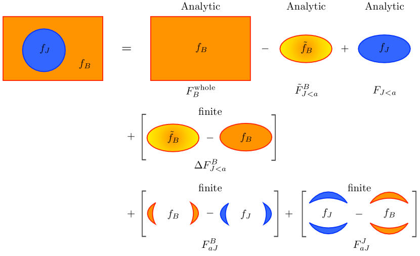
Refer to caption
Figure -1373: The general adapted version of the hemisphere decomposition for the case of a beam-jet dipole (i=a𝑖𝑎i=a, j=J𝑗𝐽j=J). The first line represents terms which can be calculated analytically, while the second and third line contain finite, numerical corrections which vanish in the small R𝑅R limit.

The term FBwholesuperscriptsubscript𝐹𝐵wholeF_{B}^{\text{whole}} corresponds to the measurement of the beam observable within the complete phase space without constraints due to the jet region. In the context of ppL+1𝑝𝑝𝐿1pp\to L+1 jet this correction was calculated in Kolodrubetz:2016dzb for the measurements in eq. (4.1) and denoted by SBsubscript𝑆𝐵S_{B} therein.888For an energy veto at e+esuperscript𝑒superscript𝑒e^{+}e^{-} collisions the associated “inclusive” correction to the one-loop soft function has been first computed in Ellis:2010rwa . For pp𝑝𝑝absentpp\to dijets also the correction from the jet-jet dipole can be calculated for a pTsubscript𝑝𝑇p_{T}-veto Hornig:2016ahz . The bare corrections are given by

SaJwhole,τ({kl},ηJ)subscriptsuperscript𝑆whole𝜏𝑎𝐽subscript𝑘𝑙subscript𝜂𝐽\displaystyle S^{{\rm whole},\tau}_{aJ}(\{k_{l}\},\eta_{J}) =αs4πδ(kJ){16ηJθ(ηJ)1μ0(kBμ)+δ(kB)[8ηJϵθ(ηJ)\displaystyle=\frac{\alpha_{s}}{4\pi}\,\delta(k_{J})\biggl{\{}16\eta_{J}\,\theta(-\eta_{J})\frac{1}{\mu}\,{\mathcal{L}}_{0}\Bigl{(}\frac{k_{B}}{\mu}\Bigr{)}+\delta(k_{B})\Bigl{[}-\frac{8\eta_{J}}{\epsilon}\,\theta(-\eta_{J})
4Li2(e2|ηJ|)8ηJ2θ(ηJ)]+𝒪(ϵ)},\displaystyle\quad-4\,\textrm{Li}_{2}\bigl{(}e^{-2|\eta_{J}|}\bigr{)}-8\eta_{J}^{2}\,\theta(-\eta_{J})\Bigr{]}+\mathcal{O}(\epsilon)\biggr{\}}\,,
SaJwhole,C({kl},ηJ)subscriptsuperscript𝑆whole𝐶𝑎𝐽subscript𝑘𝑙subscript𝜂𝐽\displaystyle S^{{\rm whole},C}_{aJ}(\{k_{l}\},\eta_{J}) =αs4πδ(kJ){8ln(1+tanhηJ2)1μ0(kBμ)+δ(kB)[4ϵln(1+tanhηJ2)\displaystyle=\frac{\alpha_{s}}{4\pi}\,\delta(k_{J})\biggl{\{}8\ln\Bigl{(}\frac{1+\tanh\eta_{J}}{2}\Bigr{)}\frac{1}{\mu}\,{\mathcal{L}}_{0}\Bigl{(}\frac{k_{B}}{\mu}\Bigr{)}+\delta(k_{B})\biggl{[}-\frac{4}{\epsilon}\ln\Bigl{(}\frac{1+\tanh\eta_{J}}{2}\Bigr{)}
+4Li2(1+tanhηJ2)+2ln2(1tanhηJ2)8ln2(2coshηJ)2π23]\displaystyle\quad+4\,\textrm{Li}_{2}\Bigl{(}\frac{1+\tanh\eta_{J}}{2}\Bigr{)}+2\ln^{2}\Bigl{(}\frac{1-\tanh\eta_{J}}{2}\Bigr{)}-8\ln^{2}(2\cosh\eta_{J})-\frac{2\pi^{2}}{3}\biggr{]}
+𝒪(ϵ)},\displaystyle\quad+\mathcal{O}(\epsilon)\biggr{\}}\,,
SaJwhole,pT({kl},ηJ)subscriptsuperscript𝑆wholesubscript𝑝𝑇𝑎𝐽subscript𝑘𝑙subscript𝜂𝐽\displaystyle S^{{\rm whole},p_{T}}_{aJ}(\{k_{l}\},\eta_{J}) =αs4πδ(kJ){1μ0(kBμ)[8η+4ϵ8ln(νeηJμ)]\displaystyle=\frac{\alpha_{s}}{4\pi}\,\delta(k_{J})\biggl{\{}\frac{1}{\mu}\,{\mathcal{L}}_{0}\Bigl{(}\frac{k_{B}}{\mu}\Bigr{)}\biggl{[}-\frac{8}{\eta}+\frac{4}{\epsilon}-8\ln\Bigl{(}\frac{\nu e^{-\eta_{J}}}{\mu}\Bigr{)}\biggr{]}
+δ(kB)[4ηϵ4ϵ2+4ϵln(νeηJμ)+π23]+𝒪(η,ϵ)}.\displaystyle\quad+\delta(k_{B})\biggl{[}\frac{4}{\eta\,\epsilon}-\frac{4}{\epsilon^{2}}+\frac{4}{\epsilon}\ln\Bigl{(}\frac{\nu e^{-\eta_{J}}}{\mu}\Bigr{)}+\frac{\pi^{2}}{3}\biggr{]}+\mathcal{O}(\eta,\epsilon)\biggr{\}}\,. (74)

The measurement of the beam region observable leads to a different divergent behavior for radiation collinear to the jet axis than for the jet measurement. This requires the computation of the analytic piece F~J<aBsuperscriptsubscript~𝐹𝐽𝑎𝐵-\tilde{F}_{J<a}^{B} (in the jet hemisphere) to correct for this mismatch. For its calculation we employ a measurement 𝒯~Bsubscript~𝒯𝐵\tilde{{\mathcal{T}}}_{B} which is linear in the momentum component napsubscript𝑛𝑎𝑝n_{a}\cdot p and identical to the beam observable 𝒯Bsubscript𝒯𝐵{\mathcal{T}}_{B} in the vicinity of nJsubscript𝑛𝐽n_{J} (i.e. for ηηJ𝜂subscript𝜂𝐽\eta\to\eta_{J}), see eq. (72). In dimensional regularization the associated correction gives just the result for the hemisphere contribution in Jouttenus:2011wh (with an appropriate rescaling factor),

S~J<aB({kl},R,ηJ)subscriptsuperscript~𝑆𝐵𝐽𝑎subscript𝑘𝑙𝑅subscript𝜂𝐽\displaystyle\tilde{S}^{B}_{J<a}(\{k_{l}\},R,\eta_{J}) =αs4πδ(kJ){8RμfB(ηJ)1(kBRμfB(ηJ))4ϵRμfB(ηJ)0(kBRμfB(ηJ))\displaystyle=\frac{\alpha_{s}}{4\pi}\,\delta(k_{J})\biggl{\{}\frac{8R}{\mu\,f_{B}(\eta_{J})}\,{\mathcal{L}}_{1}\biggl{(}\frac{k_{B}R}{\mu\,f_{B}(\eta_{J})}\biggr{)}-\frac{4}{\epsilon}\,\frac{R}{\mu\,f_{B}(\eta_{J})}\,{\mathcal{L}}_{0}\biggl{(}\frac{k_{B}R}{\mu\,f_{B}(\eta_{J})}\biggr{)}
+[2ϵ2π26]δ(kB)}.\displaystyle\quad+\biggl{[}\frac{2}{\epsilon^{2}}-\frac{\pi^{2}}{6}\biggr{]}\delta(k_{B})\biggr{\}}\,. (75)

The term FJ<asubscript𝐹𝐽𝑎F_{J<a} corresponds to the measurement of the jet observable in the rescaled jet hemisphere. The results for the angularities defined in eq. (59) can be obtained analytically from the hemisphere results in eqs. (42) and (3) and a finite correction coming from eq. (3). The latter accounts for the difference of the boost invariant jet angularity in eq. (59) from the generic definition in eq. (37) and is calculated in app. A. In total we obtain

SJ<aβ1({kl},R,ηJ)subscriptsuperscript𝑆𝛽1𝐽𝑎subscript𝑘𝑙𝑅subscript𝜂𝐽\displaystyle S^{\beta\neq 1}_{J<a}(\{k_{l}\},R,\eta_{J}) =αs4πδ(kB)β1{8μRβ11(kJμRβ1)4ϵ1μRβ10(kJμRβ1)\displaystyle=\frac{\alpha_{s}}{4\pi}\,\frac{\delta(k_{B})}{\beta\!-\!1}\biggl{\{}\frac{8}{\mu\,R^{\beta-1}}\,\mathcal{L}_{1}\biggl{(}\frac{k_{J}}{\mu\,R^{\beta-1}}\biggr{)}\!-\!\frac{4}{\epsilon}\frac{1}{\mu\,R^{\beta-1}}\,\mathcal{L}_{0}\biggl{(}\frac{k_{J}}{\mu\,R^{\beta-1}}\biggr{)} (76)
+δ(kJ)(2ϵ2π262(β1)(β2)θ(R1)ln2R)+𝒪(ϵ)},\displaystyle\quad+\delta(k_{J})\biggl{(}\frac{2}{\epsilon^{2}}-\frac{\pi^{2}}{6}-2(\beta-1)(\beta-2)\,\theta(R-1)\ln^{2}R\biggr{)}+\mathcal{O}(\epsilon)\biggr{\}}\,,
SJ<aβ=1({kl},R,ηJ)subscriptsuperscript𝑆𝛽1𝐽𝑎subscript𝑘𝑙𝑅subscript𝜂𝐽\displaystyle S^{\beta=1}_{J<a}(\{k_{l}\},R,\eta_{J}) =αs4πδ(kB){8μ1(kJμ)8μ0(kJμ)[1η+ln(νR2μcoshηJ)]\displaystyle=\frac{\alpha_{s}}{4\pi}\,\delta(k_{B})\biggl{\{}\frac{8}{\mu}\,\mathcal{L}_{1}\biggl{(}\frac{k_{J}}{\mu}\biggr{)}-\frac{8}{\mu}\,\mathcal{L}_{0}\biggl{(}\frac{k_{J}}{\mu}\biggr{)}\biggl{[}\frac{1}{\eta}+\ln\biggl{(}\frac{\nu R}{2\mu\cosh\eta_{J}}\biggl{)}\biggr{]} (77)
+δ(kJ)(4ηϵ2ϵ2+4ϵln(νR2μcoshηJ)+π26+2θ(R1)ln2R)\displaystyle\quad+\delta(k_{J})\biggl{(}\frac{4}{\eta\,\epsilon}-\frac{2}{\epsilon^{2}}+\frac{4}{\epsilon}\ln\biggl{(}\frac{\nu R}{2\mu\cosh\eta_{J}}\biggl{)}+\frac{\pi^{2}}{6}+2\,\theta(R-1)\ln^{2}R\biggr{)}
+𝒪(η,ϵ)}.\displaystyle\quad+\mathcal{O}(\eta,\epsilon)\biggr{\}}\,.

The analytic contributions in the small R limit are given by

SaJ({kl},R,ηJ)=SaJwhole({kl},ηJ)+S~J<aB({kl},R,ηJ)+SJ<a({kl},R,ηJ)+𝒪(R1,2)subscript𝑆𝑎𝐽subscript𝑘𝑙𝑅subscript𝜂𝐽subscriptsuperscript𝑆whole𝑎𝐽subscript𝑘𝑙subscript𝜂𝐽subscriptsuperscript~𝑆𝐵𝐽𝑎subscript𝑘𝑙𝑅subscript𝜂𝐽subscript𝑆𝐽𝑎subscript𝑘𝑙𝑅subscript𝜂𝐽𝒪superscript𝑅12\displaystyle S_{aJ}(\{k_{l}\},R,\eta_{J})=S^{\rm whole}_{aJ}(\{k_{l}\},\eta_{J})+\tilde{S}^{B}_{J<a}(\{k_{l}\},R,\eta_{J})+S_{J<a}(\{k_{l}\},R,\eta_{J})+{\cal O}(R^{1,2}) (78)

where the displayed terms are 𝒪(R0)𝒪superscript𝑅0{\cal O}(R^{0}) corrections and depend only logarithmically on R𝑅R. They are independent of the specific partitioning (jet definition), and for R1much-less-than𝑅1R\ll 1 yield the full result up to power corrections. In the context of an effective theory for a small jet radius the soft radiation is factorized into different types of soft modes Chien:2015cka ; Becher:2015hka ; Hornig:2016ahz ; Kolodrubetz:2016dzb . The measurement FBwholesuperscriptsubscript𝐹𝐵wholeF_{B}^{\text{whole}} applies to wide-angle soft radiation, which does not resolve the jet region but depends on the Wilson line of the jet. The corrections S~J<aBsubscriptsuperscript~𝑆𝐵𝐽𝑎\tilde{S}^{B}_{J<a} and SJ<asubscript𝑆𝐽𝑎S_{J<a} correspond to the results for the matrix elements of “soft-collinear” and “collinear-soft” modes, respectively, in the nomenclature of ref. Chien:2015cka . These are boosted and constrained by the jet boundary. In the limit R1much-less-than𝑅1R\ll 1 the beam-jet dipoles give the same results, SaJ=SbJsubscript𝑆𝑎𝐽subscript𝑆𝑏𝐽S_{aJ}=S_{bJ}, and the Wilson lines from the beams a𝑎a and b𝑏b fuse giving a total color factor 𝐓J(𝐓a+𝐓b)=𝐓J2subscript𝐓𝐽subscript𝐓𝑎subscript𝐓𝑏subscriptsuperscript𝐓2𝐽{\bf T}_{J}\cdot({\bf T}_{a}+{\bf T}_{b})=-{\bf T}^{2}_{J} Stewart:2014nna .

The measurement corrections ΔFJ<aBΔsuperscriptsubscript𝐹𝐽𝑎𝐵\Delta F_{J<a}^{B}, FaJBsubscriptsuperscript𝐹𝐵𝑎𝐽F^{B}_{aJ} and FaJJsubscriptsuperscript𝐹𝐽𝑎𝐽F^{J}_{aJ} can be in general not computed analytically, but are again finite corrections that allow for a numerical evaluation. The term ΔFJ<aBΔsuperscriptsubscript𝐹𝐽𝑎𝐵\Delta F_{J<a}^{B} corrects the subtraction in the jet hemisphere from the measurement in the beam region with f~Bsubscript~𝑓𝐵\tilde{f}_{B} to the correct observable fBsubscript𝑓𝐵f_{B}. As in sec. 3 we can write this correction in terms of an integral in η𝜂\eta-ϕitalic-ϕ\phi coordinates,

ΔSJ<aB({ki},R,ηJ)Δsubscriptsuperscript𝑆𝐵𝐽𝑎subscript𝑘𝑖𝑅subscript𝜂𝐽\displaystyle\Delta S^{B}_{J<a}(\{k_{i}\},R,\eta_{J}) =αsπΔI1,aJB(fB,R,ηJ)δ(kB)δ(kJ),absentsubscript𝛼𝑠𝜋Δsubscriptsuperscript𝐼𝐵1𝑎𝐽subscript𝑓𝐵𝑅subscript𝜂𝐽𝛿subscript𝑘𝐵𝛿subscript𝑘𝐽\displaystyle=\frac{\alpha_{s}}{\pi}\,\Delta I^{B}_{1,aJ}(f_{B},R,\eta_{J})\,\delta(k_{B})\,\delta(k_{J})\,, (79)

with

ΔI1,aJB(fB,R,ηJ)Δsubscriptsuperscript𝐼𝐵1𝑎𝐽subscript𝑓𝐵𝑅subscript𝜂𝐽\displaystyle\Delta I^{B}_{1,aJ}(f_{B},R,\eta_{J}) =12πππdϕdηeηηJcosh(ηηJ)cosϕln(eηJfB(ηJ)eηfB(η))θ(napnJpρJR)absent12𝜋superscriptsubscript𝜋𝜋differential-ditalic-ϕsuperscriptsubscriptdifferential-d𝜂superscript𝑒𝜂subscript𝜂𝐽𝜂subscript𝜂𝐽italic-ϕsuperscript𝑒subscript𝜂𝐽subscript𝑓𝐵subscript𝜂𝐽superscript𝑒𝜂subscript𝑓𝐵𝜂𝜃subscript𝑛𝑎𝑝subscript𝑛𝐽𝑝superscriptsubscript𝜌𝐽𝑅\displaystyle=\frac{1}{2\pi}\int_{-\pi}^{\pi}\mathrm{d}\phi\int_{-\infty}^{\infty}\mathrm{d}\eta\,\frac{e^{\eta-\eta_{J}}}{\cosh(\eta-\eta_{J})-\cos\phi}\,\ln\biggl{(}\frac{e^{\eta_{J}}f_{B}(\eta_{J})}{e^{\eta}f_{B}(\eta)}\biggr{)}\,\theta\Bigl{(}n_{a}\cdot p-\frac{n_{J}\cdot p}{\rho_{J}^{R}}\Bigr{)}
=θ(R1)[0R1dxh1(fB,ηJ,x)+R1R+1dxh2(fB,R,ηJ,x)]absent𝜃𝑅1delimited-[]subscriptsuperscript𝑅10differential-d𝑥subscript1subscript𝑓𝐵subscript𝜂𝐽𝑥subscriptsuperscript𝑅1𝑅1differential-d𝑥subscript2subscript𝑓𝐵𝑅subscript𝜂𝐽𝑥\displaystyle=\theta(R-1)\biggl{[}\int^{R-1}_{0}\mathrm{d}x\,h_{1}(f_{B},\eta_{J},x)+\int^{R+1}_{R-1}\mathrm{d}x\,h_{2}(f_{B},R,\eta_{J},x)\biggr{]}
+θ(1R)1RR+1dxh2(fB,R,ηJ,x),𝜃1𝑅subscriptsuperscript𝑅11𝑅differential-d𝑥subscript2subscript𝑓𝐵𝑅subscript𝜂𝐽𝑥\displaystyle\quad+\theta(1-R)\int^{R+1}_{1-R}\mathrm{d}x\,h_{2}(f_{B},R,\eta_{J},x)\,, (80)

where we have defined the integration variable xeηηJ𝑥superscript𝑒𝜂subscript𝜂𝐽x\equiv e^{\eta-\eta_{J}} and

h1(fB,ηJ,x)subscript1subscript𝑓𝐵subscript𝜂𝐽𝑥\displaystyle h_{1}(f_{B},\eta_{J},x) =2x|x21|ln(fB(ηJ)xfB(ηJ+lnx)),absent2𝑥superscript𝑥21subscript𝑓𝐵subscript𝜂𝐽𝑥subscript𝑓𝐵subscript𝜂𝐽𝑥\displaystyle=\frac{2x}{\lvert x^{2}-1\rvert}\,\ln\biggl{(}\frac{f_{B}(\eta_{J})}{xf_{B}(\eta_{J}+\ln x)}\biggr{)}\,,
h2(fB,R,ηJ,x)subscript2subscript𝑓𝐵𝑅subscript𝜂𝐽𝑥\displaystyle h_{2}(f_{B},R,\eta_{J},x) =[12πarctan(|x1|x+1(1+x)2R2R2(x1)2)]h1(fB,ηJ,x).absentdelimited-[]12𝜋𝑥1𝑥1superscript1𝑥2superscript𝑅2superscript𝑅2superscript𝑥12subscript1subscript𝑓𝐵subscript𝜂𝐽𝑥\displaystyle=\biggl{[}1-\frac{2}{\pi}\arctan\biggl{(}\frac{|x-1|}{x+1}\sqrt{\frac{(1+x)^{2}-R^{2}}{R^{2}-(x-1)^{2}}}\biggr{)}\biggr{]}\,h_{1}(f_{B},\eta_{J},x)\,. (81)

This correction depends also only on the specific shape of the hemisphere for a given value of R𝑅R, but not on the general partitioning. Since the full integrand does not exhibit singular behavior close to the jet axis (i.e. for ηηJ𝜂subscript𝜂𝐽\eta\to\eta_{J} and ϕ0italic-ϕ0\phi\to 0), it scales with the jet area for a smooth measurement in the beam region, i.e. ΔI1,aJBΔsubscriptsuperscript𝐼𝐵1𝑎𝐽\Delta I^{B}_{1,aJ} is 𝒪(R2)𝒪superscript𝑅2\mathcal{O}(R^{2}).999We have checked numerically that for the transverse momentum veto with fB(η)=1subscript𝑓𝐵𝜂1f_{B}(\eta)=1 the integral ΔI1,aJBΔsubscriptsuperscript𝐼𝐵1𝑎𝐽\Delta I^{B}_{1,aJ} vanishes for R1𝑅1R\leq 1 and gives 4ln2R4superscript2𝑅-4\ln^{2}R for R>1𝑅1R>1 as implied by the full analytic hemisphere result in eq. (3).

The terms FaJBsubscriptsuperscript𝐹𝐵𝑎𝐽F^{B}_{aJ} and FaJJsubscriptsuperscript𝐹𝐽𝑎𝐽F^{J}_{aJ} correct for the difference between the actual jet definition (through the partitioning) and the employed jet hemisphere with scaling parameter ρJRsuperscriptsubscript𝜌𝐽𝑅\rho_{J}^{R}. Their contribution to the soft function directly corresponds to eq. (3). SaJBsubscriptsuperscript𝑆𝐵𝑎𝐽S^{B}_{aJ} is given by

SaJB({kl},{dn},ηJ)subscriptsuperscript𝑆𝐵𝑎𝐽subscript𝑘𝑙subscript𝑑𝑛subscript𝜂𝐽\displaystyle S^{B}_{aJ}(\{k_{l}\},\{d_{n}\},\eta_{J}) =αsπ{I0,aJB({dn},ηJ)[δ(kB)1μ0(kJμ)1μ0(kBμ)δ(kJ)]\displaystyle=\frac{\alpha_{s}}{\pi}\bigg{\{}I^{B}_{0,aJ}(\{d_{n}\},\eta_{J})\bigg{[}\delta(k_{B})\,\frac{1}{\mu}{\mathcal{L}}_{0}\Bigl{(}\frac{k_{J}}{\mu}\Bigr{)}-\frac{1}{\mu}{\mathcal{L}}_{0}\Bigl{(}\frac{k_{B}}{\mu}\Bigr{)}\,\delta(k_{J})\bigg{]}
+I1,aJB({dn},{fn},ηJ)δ(kB)δ(kJ)},\displaystyle\quad+I^{B}_{1,aJ}(\{d_{n}\},\{f_{n}\},\eta_{J})\,\delta(k_{B})\,\delta(k_{J})\bigg{\}}\,, (82)

where the relevant integrals depend now on the specific distance measures and are given by

I0,aJB({dn},ηJ)subscriptsuperscript𝐼𝐵0𝑎𝐽subscript𝑑𝑛subscript𝜂𝐽\displaystyle I^{B}_{0,aJ}(\{d_{n}\},\eta_{J}) =12πππdϕdηeηηJcosh(ηηJ)cosϕabsent12𝜋superscriptsubscript𝜋𝜋differential-ditalic-ϕsuperscriptsubscriptdifferential-d𝜂superscript𝑒𝜂subscript𝜂𝐽𝜂subscript𝜂𝐽italic-ϕ\displaystyle=\frac{1}{2\pi}\int_{-\pi}^{\pi}\mathrm{d}\phi\int_{-\infty}^{\infty}\mathrm{d}\eta\,\frac{e^{\eta-\eta_{J}}}{\cosh(\eta-\eta_{J})-\cos\phi}\, (83)
×θ(dJ(η,ϕ)dB(η))θ(R2eηJη2cosh(ηηJ)+2cosϕ),absent𝜃subscript𝑑𝐽𝜂italic-ϕsubscript𝑑𝐵𝜂𝜃superscript𝑅2superscript𝑒subscript𝜂𝐽𝜂2𝜂subscript𝜂𝐽2italic-ϕ\displaystyle\quad\times\theta\bigl{(}d_{J}(\eta,\phi)-d_{B}(\eta)\bigr{)}\,\theta\Bigl{(}R^{2}e^{\eta_{J}-\eta}-2\cosh(\eta-\eta_{J})+2\cos\phi\Bigr{)}\,,
I1,aJB({dn},{fn},ηJ)subscriptsuperscript𝐼𝐵1𝑎𝐽subscript𝑑𝑛subscript𝑓𝑛subscript𝜂𝐽\displaystyle I^{B}_{1,aJ}(\{d_{n}\},\{f_{n}\},\eta_{J}) =12πππdϕdηeηηJcosh(ηηJ)cosϕln(fB(η)fJ(η,ϕ))absent12𝜋superscriptsubscript𝜋𝜋differential-ditalic-ϕsuperscriptsubscriptdifferential-d𝜂superscript𝑒𝜂subscript𝜂𝐽𝜂subscript𝜂𝐽italic-ϕsubscript𝑓𝐵𝜂subscript𝑓𝐽𝜂italic-ϕ\displaystyle=\frac{1}{2\pi}\int_{-\pi}^{\pi}\mathrm{d}\phi\int_{-\infty}^{\infty}\mathrm{d}\eta\,\frac{e^{\eta-\eta_{J}}}{\cosh(\eta-\eta_{J})-\cos\phi}\,\ln\biggl{(}\frac{f_{B}(\eta)}{f_{J}(\eta,\phi)}\biggr{)}\,
×θ(dJ(η,ϕ)dB(η))θ(R2eηJη2cosh(ηηJ)+2cosϕ).absent𝜃subscript𝑑𝐽𝜂italic-ϕsubscript𝑑𝐵𝜂𝜃superscript𝑅2superscript𝑒subscript𝜂𝐽𝜂2𝜂subscript𝜂𝐽2italic-ϕ\displaystyle\quad\times\theta\bigl{(}d_{J}(\eta,\phi)-d_{B}(\eta)\bigr{)}\,\theta\Bigl{(}R^{2}e^{\eta_{J}-\eta}-2\cosh(\eta-\eta_{J})+2\cos\phi\Bigr{)}\,.

In analogy, SaJJsubscriptsuperscript𝑆𝐽𝑎𝐽S^{J}_{aJ} is given by

SaJJ({kl},{dn},ηJ)subscriptsuperscript𝑆𝐽𝑎𝐽subscript𝑘𝑙subscript𝑑𝑛subscript𝜂𝐽\displaystyle S^{J}_{aJ}(\{k_{l}\},\{d_{n}\},\eta_{J}) =αsπ{I0,aJJ({dn},ηJ)[δ(kJ)1μ0(kBμ)1μ0(kJμ)δ(kB)]\displaystyle=\frac{\alpha_{s}}{\pi}\bigg{\{}I^{J}_{0,aJ}(\{d_{n}\},\eta_{J})\bigg{[}\delta(k_{J})\,\frac{1}{\mu}{\mathcal{L}}_{0}\Bigl{(}\frac{k_{B}}{\mu}\Bigr{)}-\frac{1}{\mu}{\mathcal{L}}_{0}\Bigl{(}\frac{k_{J}}{\mu}\Bigr{)}\,\delta(k_{B})\bigg{]}
+I1,aJJ({dn},{fn},ηJ)δ(kB)δ(kJ)},\displaystyle\quad+I^{J}_{1,aJ}(\{d_{n}\},\{f_{n}\},\eta_{J})\,\delta(k_{B})\,\delta(k_{J})\bigg{\}}\,, (84)

with

I0,aJJ({dn},ηJ)subscriptsuperscript𝐼𝐽0𝑎𝐽subscript𝑑𝑛subscript𝜂𝐽\displaystyle I^{J}_{0,aJ}(\{d_{n}\},\eta_{J}) =12πππdϕdηeηηJcosh(ηηJ)cosϕabsent12𝜋superscriptsubscript𝜋𝜋differential-ditalic-ϕsuperscriptsubscriptdifferential-d𝜂superscript𝑒𝜂subscript𝜂𝐽𝜂subscript𝜂𝐽italic-ϕ\displaystyle=\frac{1}{2\pi}\int_{-\pi}^{\pi}\mathrm{d}\phi\int_{-\infty}^{\infty}\mathrm{d}\eta\,\frac{e^{\eta-\eta_{J}}}{\cosh(\eta-\eta_{J})-\cos\phi}\, (85)
×θ(dB(η,ϕ)dJ(η))θ(2cosh(ηηJ)2cosϕR2eηJη),absent𝜃subscript𝑑𝐵𝜂italic-ϕsubscript𝑑𝐽𝜂𝜃2𝜂subscript𝜂𝐽2italic-ϕsuperscript𝑅2superscript𝑒subscript𝜂𝐽𝜂\displaystyle\quad\times\theta\bigl{(}d_{B}(\eta,\phi)-d_{J}(\eta)\bigr{)}\,\theta\Bigl{(}2\cosh(\eta-\eta_{J})-2\cos\phi-R^{2}e^{\eta_{J}-\eta}\Bigr{)}\,,
I1,aJJ({dn},{fn},ηJ)subscriptsuperscript𝐼𝐽1𝑎𝐽subscript𝑑𝑛subscript𝑓𝑛subscript𝜂𝐽\displaystyle I^{J}_{1,aJ}(\{d_{n}\},\{f_{n}\},\eta_{J}) =12πππdϕdηeηηJcosh(ηηJ)cosϕln(fJ(η,ϕ)fB(η,ϕ))absent12𝜋superscriptsubscript𝜋𝜋differential-ditalic-ϕsuperscriptsubscriptdifferential-d𝜂superscript𝑒𝜂subscript𝜂𝐽𝜂subscript𝜂𝐽italic-ϕsubscript𝑓𝐽𝜂italic-ϕsubscript𝑓𝐵𝜂italic-ϕ\displaystyle=\frac{1}{2\pi}\int_{-\pi}^{\pi}\mathrm{d}\phi\int_{-\infty}^{\infty}\mathrm{d}\eta\,\frac{e^{\eta-\eta_{J}}}{\cosh(\eta-\eta_{J})-\cos\phi}\,\ln\biggl{(}\frac{f_{J}(\eta,\phi)}{f_{B}(\eta,\phi)}\biggr{)}\,
×θ(dB(η,ϕ)dJ(η))θ(2cosh(ηηJ)2cosϕR2eηJη).absent𝜃subscript𝑑𝐵𝜂italic-ϕsubscript𝑑𝐽𝜂𝜃2𝜂subscript𝜂𝐽2italic-ϕsuperscript𝑅2superscript𝑒subscript𝜂𝐽𝜂\displaystyle\quad\times\theta\bigl{(}d_{B}(\eta,\phi)-d_{J}(\eta)\bigr{)}\,\theta\Bigl{(}2\cosh(\eta-\eta_{J})-2\cos\phi-R^{2}e^{\eta_{J}-\eta}\Bigr{)}\,.

These integrals scale individually as 𝒪(R)𝒪𝑅\mathcal{O}(R), but yield in total 𝒪(R2)𝒪superscript𝑅2\mathcal{O}(R^{2}) contributions, as explained in app. B.2.101010This holds only for a smooth measurement in the beam region. For the beam thrust veto and |ηJ|<Rsubscript𝜂𝐽𝑅|\eta_{J}|<R the resulting total correction is of 𝒪(R)𝒪𝑅\mathcal{O}(R) due to the kink at η=0𝜂0\eta=0. We will discuss in app. B how the numerical evaluation of these integrals can be carried out efficiently by explicitly determining the integration domains. While a full analytic calculation of these does not seem feasible in general, it is possible to compute them in an expansion for RR0much-less-than𝑅subscript𝑅0R\ll R_{0} (where R0subscript𝑅0R_{0} denotes the generic convergence radius where the expansion breaks down). We calculate the terms at 𝒪(R2)𝒪superscript𝑅2\mathcal{O}(R^{2}) in app. A.2. Such an expansion has been also applied in Dasgupta:2012hg ; Liu:2014oog for the inclusive jet mass spectrum where it was found that 𝒪(R4)𝒪superscript𝑅4\mathcal{O}(R^{4}) corrections have a negligible impact for phenomenologically relevant values of R𝑅R.

4.3 Summary of corrections

To give a transparent overview of all corrections we display in the following the structure of the full (renormalized) soft functions for all combinations β1𝛽1\beta\neq 1, β=1𝛽1\beta=1 and γ=1,2𝛾12\gamma=1,2. Since eqs. (42) and (3) encode the full μ𝜇\mu- and ν𝜈\nu-dependence of the soft function, one can directly read off the counterterms for the soft function absorbing all 1/ϵ1italic-ϵ1/\epsilon- and 1/η1𝜂1/\eta-divergences. These result in the well-known one-loop anomalous dimensions for the associated soft function defined by

μddμS1κ({ki},{di},ηJ,μ,ν)𝜇dd𝜇subscriptsuperscript𝑆𝜅1subscript𝑘𝑖subscript𝑑𝑖subscript𝜂𝐽𝜇𝜈\displaystyle\mu\frac{\mathrm{d}}{\mathrm{d}\mu}S^{\kappa}_{1}(\{k_{i}\},\{d_{i}\},\eta_{J},\mu,\nu) =dkBdkJγS1κ({kiki},ηJ,μ,ν)S1κ({ki},{di},ηJ,μ,ν),absentdifferential-dsuperscriptsubscript𝑘𝐵differential-dsuperscriptsubscript𝑘𝐽subscriptsuperscript𝛾𝜅subscript𝑆1subscript𝑘𝑖superscriptsubscript𝑘𝑖subscript𝜂𝐽𝜇𝜈subscriptsuperscript𝑆𝜅1superscriptsubscript𝑘𝑖subscript𝑑𝑖subscript𝜂𝐽𝜇𝜈\displaystyle=\int\mathrm{d}k_{B}^{\prime}\,\mathrm{d}k_{J}^{\prime}\,\gamma^{\kappa}_{S_{1}}(\{k_{i}-k_{i}^{\prime}\},\eta_{J},\mu,\nu)\,S^{\kappa}_{1}(\{k_{i}^{\prime}\},\{d_{i}\},\eta_{J},\mu,\nu)\,,
νddνS1κ({ki},{di},ηJ,μ,ν)𝜈dd𝜈subscriptsuperscript𝑆𝜅1subscript𝑘𝑖subscript𝑑𝑖subscript𝜂𝐽𝜇𝜈\displaystyle\nu\frac{\mathrm{d}}{\mathrm{d}\nu}S^{\kappa}_{1}(\{k_{i}\},\{d_{i}\},\eta_{J},\mu,\nu) =dkBdkJγS1,νκ({kiki},μ)S1κ({ki},{di},ηJ,μ,ν).absentdifferential-dsuperscriptsubscript𝑘𝐵differential-dsuperscriptsubscript𝑘𝐽subscriptsuperscript𝛾𝜅subscript𝑆1𝜈subscript𝑘𝑖superscriptsubscript𝑘𝑖𝜇subscriptsuperscript𝑆𝜅1superscriptsubscript𝑘𝑖subscript𝑑𝑖subscript𝜂𝐽𝜇𝜈\displaystyle=\int\mathrm{d}k_{B}^{\prime}\,\mathrm{d}k_{J}^{\prime}\,\gamma^{\kappa}_{S_{1},\nu}(\{k_{i}-k_{i}^{\prime}\},\mu)\,S^{\kappa}_{1}(\{k_{i}^{\prime}\},\{d_{i}\},\eta_{J},\mu,\nu)\,. (86)

The ν𝜈\nu-anomalous dimension is only present for β=1𝛽1\beta=1 or γ=1𝛾1\gamma=1. The explicit one-loop expressions for all cases read

γS1,β1,γ=2κ(1)({ki},ηJ,μ)subscriptsuperscript𝛾𝜅1formulae-sequencesubscript𝑆1𝛽1𝛾2subscript𝑘𝑖subscript𝜂𝐽𝜇\displaystyle\gamma^{\kappa(1)}_{S_{1},\beta\neq 1,\gamma=2}(\{k_{i}\},\eta_{J},\mu) =αs(μ)4π 2Γ0{𝐓J21β11μ0(kJμ)δ(kB)\displaystyle=\frac{\alpha_{s}(\mu)}{4\pi}\,2\Gamma_{0}\biggl{\{}{\bf T}_{J}^{2}\,\frac{1}{\beta-1}\,\frac{1}{\mu}\,{\mathcal{L}}_{0}\Bigl{(}\frac{k_{J}}{\mu}\Bigr{)}\,\delta(k_{B})
+(𝐓a2+𝐓b2)1μ0(kBμ)δ(kJ)+(𝐓a2𝐓b2)ηJδ(kJ)δ(kB)},\displaystyle\quad+({\bf T}_{a}^{2}+{\bf T}_{b}^{2})\,\frac{1}{\mu}\,{\mathcal{L}}_{0}\Bigl{(}\frac{k_{B}}{\mu}\Bigr{)}\,\delta(k_{J})+({\bf T}_{a}^{2}-{\bf T}_{b}^{2})\,\eta_{J}\,\delta(k_{J})\,\delta(k_{B})\biggr{\}}\,,
γS1,β1,γ=1κ(1)({ki},ηJ,μ,ν)subscriptsuperscript𝛾𝜅1formulae-sequencesubscript𝑆1𝛽1𝛾1subscript𝑘𝑖subscript𝜂𝐽𝜇𝜈\displaystyle\gamma^{\kappa(1)}_{S_{1},\beta\neq 1,\gamma=1}(\{k_{i}\},\eta_{J},\mu,\nu) =αs(μ)4π 2Γ0{𝐓J21β11μ0(kJμ)δ(kB)\displaystyle=\frac{\alpha_{s}(\mu)}{4\pi}\,2\Gamma_{0}\biggl{\{}{\bf T}_{J}^{2}\,\frac{1}{\beta-1}\,\frac{1}{\mu}\,{\mathcal{L}}_{0}\Bigl{(}\frac{k_{J}}{\mu}\Bigr{)}\delta(k_{B})
+[(𝐓a2+𝐓b2)ln(νμ)+(𝐓a2𝐓b2)ηJ]δ(kJ)δ(kB)},\displaystyle\quad+\Bigl{[}-({\bf T}_{a}^{2}+{\bf T}_{b}^{2})\ln\Bigl{(}\frac{\nu}{\mu}\Bigr{)}+({\bf T}_{a}^{2}-{\bf T}_{b}^{2})\,\eta_{J}\Bigr{]}\,\delta(k_{J})\,\delta(k_{B})\biggr{\}}\,,
γS1,β=1,γ=2κ(1)({ki},ηJ,μ,ν)subscriptsuperscript𝛾𝜅1formulae-sequencesubscript𝑆1𝛽1𝛾2subscript𝑘𝑖subscript𝜂𝐽𝜇𝜈\displaystyle\gamma^{\kappa(1)}_{S_{1},\beta=1,\gamma=2}(\{k_{i}\},\eta_{J},\mu,\nu) =αs(μ)4π 2Γ0{(𝐓a2+𝐓b2)1μ0(kBμ)δ(kJ)\displaystyle=\frac{\alpha_{s}(\mu)}{4\pi}\,2\Gamma_{0}\biggl{\{}({\bf T}_{a}^{2}+{\bf T}_{b}^{2})\,\frac{1}{\mu}\,{\mathcal{L}}_{0}\Bigl{(}\frac{k_{B}}{\mu}\Bigr{)}\,\delta(k_{J})
+[𝐓J2ln(ν2μcoshηJ)+(𝐓a2𝐓b2)ηJ]δ(kJ)δ(kB)},\displaystyle\quad+\Bigl{[}-{\bf T}_{J}^{2}\ln\Bigl{(}\frac{\nu}{2\mu\cosh\eta_{J}}\Bigr{)}+({\bf T}_{a}^{2}-{\bf T}_{b}^{2})\,\eta_{J}\Bigr{]}\,\delta(k_{J})\,\delta(k_{B})\biggr{\}}\,,
γS1,β=1,γ=1κ(1)({ki},ηJ,μ,ν)subscriptsuperscript𝛾𝜅1formulae-sequencesubscript𝑆1𝛽1𝛾1subscript𝑘𝑖subscript𝜂𝐽𝜇𝜈\displaystyle\gamma^{\kappa(1)}_{S_{1},\beta=1,\gamma=1}(\{k_{i}\},\eta_{J},\mu,\nu) =αs(μ)4π 2Γ0δ(kJ)δ(kB){(𝐓a2+𝐓b2+𝐓J2)ln(νμ)\displaystyle=\frac{\alpha_{s}(\mu)}{4\pi}\,2\Gamma_{0}\,\delta(k_{J})\,\delta(k_{B})\biggl{\{}-({\bf T}_{a}^{2}+{\bf T}_{b}^{2}+{\bf T}_{J}^{2})\ln\Bigl{(}\frac{\nu}{\mu}\Bigr{)}
+𝐓J2ln(2coshηJ)+(𝐓a2𝐓b2)ηJ},\displaystyle\quad+{\bf T}_{J}^{2}\ln(2\cosh\eta_{J})+({\bf T}_{a}^{2}-{\bf T}_{b}^{2})\,\eta_{J}\biggr{\}}\,, (87)

for the μ𝜇\mu-anomalous dimensions with Γ0=4subscriptΓ04\Gamma_{0}=4 being the coefficient of the one-loop cusp anomalous dimension. The ν𝜈\nu-anomalous dimensions are given by

γS1,ν,β1,γ=1κ(1)({ki},μ)subscriptsuperscript𝛾𝜅1formulae-sequencesubscript𝑆1𝜈𝛽1𝛾1subscript𝑘𝑖𝜇\displaystyle\gamma^{\kappa(1)}_{S_{1},\nu,\beta\neq 1,\gamma=1}(\{k_{i}\},\mu) =αs(μ)4π 2Γ0(𝐓a2+𝐓b2)1μ0(kBμ)δ(kJ),absentsubscript𝛼𝑠𝜇4𝜋2subscriptΓ0superscriptsubscript𝐓𝑎2superscriptsubscript𝐓𝑏21𝜇subscript0subscript𝑘𝐵𝜇𝛿subscript𝑘𝐽\displaystyle=\frac{\alpha_{s}(\mu)}{4\pi}\,2\Gamma_{0}({\bf T}_{a}^{2}+{\bf T}_{b}^{2})\,\frac{1}{\mu}\,{\mathcal{L}}_{0}\Bigl{(}\frac{k_{B}}{\mu}\Bigr{)}\,\delta(k_{J})\,, (88)
γS1,ν,β=1,γ=2κ(1)({ki},μ)subscriptsuperscript𝛾𝜅1formulae-sequencesubscript𝑆1𝜈𝛽1𝛾2subscript𝑘𝑖𝜇\displaystyle\gamma^{\kappa(1)}_{S_{1},\nu,\beta=1,\gamma=2}(\{k_{i}\},\mu) =αs(μ)4π 2Γ0𝐓J21μ0(kJμ)δ(kB),absentsubscript𝛼𝑠𝜇4𝜋2subscriptΓ0superscriptsubscript𝐓𝐽21𝜇subscript0subscript𝑘𝐽𝜇𝛿subscript𝑘𝐵\displaystyle=\frac{\alpha_{s}(\mu)}{4\pi}\,2\Gamma_{0}\,{\bf T}_{J}^{2}\,\frac{1}{\mu}\,{\mathcal{L}}_{0}\Bigl{(}\frac{k_{J}}{\mu}\Bigr{)}\,\delta(k_{B})\,,
γS1,ν,β=1,γ=1κ(1)({ki},μ)subscriptsuperscript𝛾𝜅1formulae-sequencesubscript𝑆1𝜈𝛽1𝛾1subscript𝑘𝑖𝜇\displaystyle\gamma^{\kappa(1)}_{S_{1},\nu,\beta=1,\gamma=1}(\{k_{i}\},\mu) =αs(μ)4π 2Γ0{(𝐓a2+𝐓b2)1μ0(kBμ)δ(kJ)+𝐓J21μ0(kJμ)δ(kB)}.absentsubscript𝛼𝑠𝜇4𝜋2subscriptΓ0superscriptsubscript𝐓𝑎2superscriptsubscript𝐓𝑏21𝜇subscript0subscript𝑘𝐵𝜇𝛿subscript𝑘𝐽superscriptsubscript𝐓𝐽21𝜇subscript0subscript𝑘𝐽𝜇𝛿subscript𝑘𝐵\displaystyle=\frac{\alpha_{s}(\mu)}{4\pi}\,2\Gamma_{0}\,\biggl{\{}({\bf T}_{a}^{2}+{\bf T}_{b}^{2})\,\frac{1}{\mu}\,{\mathcal{L}}_{0}\Bigl{(}\frac{k_{B}}{\mu}\Bigr{)}\,\delta(k_{J})+{\bf T}_{J}^{2}\,\frac{1}{\mu}\,{\mathcal{L}}_{0}\Bigl{(}\frac{k_{J}}{\mu}\Bigr{)}\,\delta(k_{B})\biggr{\}}\,.

For β1𝛽1\beta\neq 1 and γ=2𝛾2\gamma=2, i.e. SCETIsubscriptSCETI{\rm SCET}_{\rm I} jet and beams, the renormalized result for the one-loop soft function reads

S1,β1,γ=2κ(1)({ki},{di},ηJ,μ)=αs(μ)4π{𝐓a𝐓b[16μ1(kBμ)δ(kJ)\displaystyle S^{\kappa(1)}_{1,\beta\neq 1,\gamma=2}(\{k_{i}\},\{d_{i}\},\eta_{J},\mu)=\frac{\alpha_{s}(\mu)}{4\pi}\biggl{\{}{\bf T}_{a}\cdot{\bf T}_{b}\biggl{[}\frac{16}{\mu}\,{\mathcal{L}}_{1}\Bigl{(}\frac{k_{B}}{\mu}\Bigr{)}\,\delta(k_{J})
+sab,B({di},ηJ)(1μ0(kBμ)δ(kJ)1μ0(kJμ)δ(kB))+sab,δ({di},{fi},ηJ)δ(kB)δ(kJ)]\displaystyle\quad+s_{ab,B}(\{d_{i}\},\eta_{J})\Bigl{(}\frac{1}{\mu}{\mathcal{L}}_{0}\Bigl{(}\frac{k_{B}}{\mu}\Bigr{)}\delta(k_{J})-\frac{1}{\mu}{\mathcal{L}}_{0}\Bigl{(}\frac{k_{J}}{\mu}\Bigr{)}\delta(k_{B})\Bigr{)}+s_{ab,\delta}(\{d_{i}\},\{f_{i}\},\eta_{J})\,\delta(k_{B})\,\delta(k_{J})\biggr{]}
+𝐓a𝐓J[1β18μ1(kJμ)δ(kB)+8μ1(kBμ)δ(kJ)\displaystyle\quad+{\bf T}_{a}\cdot{\bf T}_{J}\biggl{[}\frac{1}{\beta-1}\,\frac{8}{\mu}\,{\mathcal{L}}_{1}\Bigl{(}\frac{k_{J}}{\mu}\Bigr{)}\,\delta(k_{B})+\frac{8}{\mu}\,{\mathcal{L}}_{1}\Bigl{(}\frac{k_{B}}{\mu}\Bigr{)}\,\delta(k_{J})
+saJ,B({di},ηJ)1μ0(kBμ)δ(kJ)+saJ,J({di},ηJ)1μ0(kJμ)δ(kB)subscript𝑠𝑎𝐽𝐵subscript𝑑𝑖subscript𝜂𝐽1𝜇subscript0subscript𝑘𝐵𝜇𝛿subscript𝑘𝐽subscript𝑠𝑎𝐽𝐽subscript𝑑𝑖subscript𝜂𝐽1𝜇subscript0subscript𝑘𝐽𝜇𝛿subscript𝑘𝐵\displaystyle\quad+s_{aJ,B}(\{d_{i}\},\eta_{J})\,\frac{1}{\mu}\,{\mathcal{L}}_{0}\Bigl{(}\frac{k_{B}}{\mu}\Bigr{)}\,\delta(k_{J})+s_{aJ,J}(\{d_{i}\},\eta_{J})\,\frac{1}{\mu}\,{\mathcal{L}}_{0}\Bigl{(}\frac{k_{J}}{\mu}\Bigr{)}\,\delta(k_{B})
+saJ,δ({di},{fi},ηJ)δ(kJ)δ(kB)]+𝐓b𝐓J[ηJηJ]},\displaystyle\quad+s_{aJ,\delta}(\{d_{i}\},\{f_{i}\},\eta_{J})\,\delta(k_{J})\,\delta(k_{B})\biggr{]}+{\bf T}_{b}\cdot{\bf T}_{J}\biggl{[}\eta_{J}\leftrightarrow-\eta_{J}\biggr{]}\biggr{\}}\,, (89)

For β1𝛽1\beta\neq 1 and γ=1𝛾1\gamma=1, i.e. a SCETIsubscriptSCETI{\rm SCET}_{\rm I} jet and SCETIIsubscriptSCETII{\rm SCET}_{\rm II} beams, the result reads

S1,β1,γ=1κ(1)({ki},{di},ηJ,μ,ν)=αs(μ)4π{𝐓a𝐓b[16μ1(kBμ)δ(kJ)16μ0(kBμ)ln(νμ)δ(kJ)\displaystyle S^{\kappa(1)}_{1,\beta\neq 1,\gamma=1}(\{k_{i}\},\{d_{i}\},\eta_{J},\mu,\nu)=\frac{\alpha_{s}(\mu)}{4\pi}\biggl{\{}{\bf T}_{a}\cdot{\bf T}_{b}\biggl{[}\frac{16}{\mu}\,{\mathcal{L}}_{1}\Bigl{(}\frac{k_{B}}{\mu}\Bigr{)}\,\delta(k_{J})-\frac{16}{\mu}\,{\mathcal{L}}_{0}\Bigl{(}\frac{k_{B}}{\mu}\Bigr{)}\ln\Bigl{(}\frac{\nu}{\mu}\Bigr{)}\,\delta(k_{J})
+sab,B({di},ηJ)(1μ0(kBμ)δ(kJ)1μ0(kJμ)δ(kB))+sab,δ({di},{fi},ηJ)δ(kB)δ(kJ)]\displaystyle\quad+s_{ab,B}(\{d_{i}\},\eta_{J})\Bigl{(}\frac{1}{\mu}{\mathcal{L}}_{0}\Bigl{(}\frac{k_{B}}{\mu}\Bigr{)}\delta(k_{J})-\frac{1}{\mu}{\mathcal{L}}_{0}\Bigl{(}\frac{k_{J}}{\mu}\Bigr{)}\delta(k_{B})\Bigr{)}+s_{ab,\delta}(\{d_{i}\},\{f_{i}\},\eta_{J})\,\delta(k_{B})\,\delta(k_{J})\biggr{]}
+𝐓a𝐓J[1β18μ1(kJμ)δ(kB)+8μ1(kBμ)δ(kJ)8μ0(kBμ)ln(νμ)δ(kJ)\displaystyle\quad+{\bf T}_{a}\cdot{\bf T}_{J}\biggl{[}\frac{1}{\beta-1}\,\frac{8}{\mu}\,{\mathcal{L}}_{1}\Bigl{(}\frac{k_{J}}{\mu}\Bigr{)}\,\delta(k_{B})+\frac{8}{\mu}\,{\mathcal{L}}_{1}\Bigl{(}\frac{k_{B}}{\mu}\Bigr{)}\,\delta(k_{J})-\frac{8}{\mu}\,\mathcal{L}_{0}\Bigl{(}\frac{k_{B}}{\mu}\Bigr{)}\ln\Bigl{(}\frac{\nu}{\mu}\Bigr{)}\,\delta(k_{J})
+saJ,B({di},ηJ)1μ0(kBμ)δ(kJ)+saJ,J({di},ηJ)1μ0(kJμ)δ(kB)subscript𝑠𝑎𝐽𝐵subscript𝑑𝑖subscript𝜂𝐽1𝜇subscript0subscript𝑘𝐵𝜇𝛿subscript𝑘𝐽subscript𝑠𝑎𝐽𝐽subscript𝑑𝑖subscript𝜂𝐽1𝜇subscript0subscript𝑘𝐽𝜇𝛿subscript𝑘𝐵\displaystyle\quad+s_{aJ,B}(\{d_{i}\},\eta_{J})\,\frac{1}{\mu}\,{\mathcal{L}}_{0}\Bigl{(}\frac{k_{B}}{\mu}\Bigr{)}\,\delta(k_{J})+s_{aJ,J}(\{d_{i}\},\eta_{J})\,\frac{1}{\mu}\,{\mathcal{L}}_{0}\Bigl{(}\frac{k_{J}}{\mu}\Bigr{)}\,\delta(k_{B})
+saJ,δ({di},{fi},ηJ)δ(kJ)δ(kB)]+𝐓b𝐓J[ηJηJ]},\displaystyle\quad+s_{aJ,\delta}(\{d_{i}\},\{f_{i}\},\eta_{J})\,\delta(k_{J})\,\delta(k_{B})\biggr{]}+{\bf T}_{b}\cdot{\bf T}_{J}\biggl{[}\eta_{J}\leftrightarrow-\eta_{J}\biggr{]}\biggr{\}}\,, (90)

For β=1𝛽1\beta=1 and γ=2𝛾2\gamma=2, i.e. a SCETIIsubscriptSCETII{\rm SCET}_{\rm II} jet and SCETIsubscriptSCETI{\rm SCET}_{\rm I} beams, the result reads

S1,β=1,γ=2κ(1)({ki},{di},ηJ,μ,ν)=αs(μ)4π{𝐓a𝐓b[16μ1(kBμ)δ(kJ)\displaystyle S^{\kappa(1)}_{1,\beta=1,\gamma=2}(\{k_{i}\},\{d_{i}\},\eta_{J},\mu,\nu)=\frac{\alpha_{s}(\mu)}{4\pi}\biggl{\{}{\bf T}_{a}\cdot{\bf T}_{b}\biggl{[}\frac{16}{\mu}\,{\mathcal{L}}_{1}\Bigl{(}\frac{k_{B}}{\mu}\Bigr{)}\,\delta(k_{J})
+sab,B({di},ηJ)(1μ0(kBμ)δ(kJ)1μ0(kJμ)δ(kB))+sab,δ({di},{fi},ηJ)δ(kB)δ(kJ)]\displaystyle\quad+s_{ab,B}(\{d_{i}\},\eta_{J})\Bigl{(}\frac{1}{\mu}{\mathcal{L}}_{0}\Bigl{(}\frac{k_{B}}{\mu}\Bigr{)}\delta(k_{J})-\frac{1}{\mu}{\mathcal{L}}_{0}\Bigl{(}\frac{k_{J}}{\mu}\Bigr{)}\delta(k_{B})\Bigr{)}+s_{ab,\delta}(\{d_{i}\},\{f_{i}\},\eta_{J})\,\delta(k_{B})\,\delta(k_{J})\biggr{]}
+𝐓a𝐓J[8μ1(kJμ)δ(kB)8μ0(kJμ)ln(ν2μcoshηJ)δ(kB)+8μ1(kBμ)δ(kJ)\displaystyle\quad+{\bf T}_{a}\cdot{\bf T}_{J}\biggl{[}\frac{8}{\mu}\,\mathcal{L}_{1}\biggl{(}\frac{k_{J}}{\mu}\biggr{)}\,\delta(k_{B})-\frac{8}{\mu}\,\mathcal{L}_{0}\biggl{(}\frac{k_{J}}{\mu}\biggr{)}\ln\biggl{(}\frac{\nu}{2\mu\cosh\eta_{J}}\biggl{)}\,\delta(k_{B})+\frac{8}{\mu}\,{\mathcal{L}}_{1}\Bigl{(}\frac{k_{B}}{\mu}\Bigr{)}\,\delta(k_{J})
+saJ,B({di},ηJ)1μ0(kBμ)δ(kJ)+saJ,J({di},ηJ)1μ0(kJμ)δ(kB)subscript𝑠𝑎𝐽𝐵subscript𝑑𝑖subscript𝜂𝐽1𝜇subscript0subscript𝑘𝐵𝜇𝛿subscript𝑘𝐽subscript𝑠𝑎𝐽𝐽subscript𝑑𝑖subscript𝜂𝐽1𝜇subscript0subscript𝑘𝐽𝜇𝛿subscript𝑘𝐵\displaystyle\quad+s_{aJ,B}(\{d_{i}\},\eta_{J})\,\frac{1}{\mu}\,{\mathcal{L}}_{0}\Bigl{(}\frac{k_{B}}{\mu}\Bigr{)}\,\delta(k_{J})+s_{aJ,J}(\{d_{i}\},\eta_{J})\,\frac{1}{\mu}\,{\mathcal{L}}_{0}\Bigl{(}\frac{k_{J}}{\mu}\Bigr{)}\,\delta(k_{B})
+saJ,δ({di},{fi},ηJ)δ(kJ)δ(kB)]+𝐓b𝐓J[ηJηJ]},\displaystyle\quad+s_{aJ,\delta}(\{d_{i}\},\{f_{i}\},\eta_{J})\,\delta(k_{J})\,\delta(k_{B})\biggr{]}+{\bf T}_{b}\cdot{\bf T}_{J}\biggl{[}\eta_{J}\leftrightarrow-\eta_{J}\biggr{]}\biggr{\}}\,, (91)

For β=1𝛽1\beta=1 and γ=1𝛾1\gamma=1, i.e. SCETIIsubscriptSCETII{\rm SCET}_{\rm II} jet and beams, the result reads

S1,β=1,γ=1κ(1)({ki},{di},ηJ,μ,ν)=αs(μ)4π{𝐓a𝐓b[16μ1(kBμ)δ(kJ)16μ0(kBμ)ln(νμ)δ(kJ)\displaystyle S^{\kappa(1)}_{1,\beta=1,\gamma=1}(\{k_{i}\},\{d_{i}\},\eta_{J},\mu,\nu)=\frac{\alpha_{s}(\mu)}{4\pi}\biggl{\{}{\bf T}_{a}\cdot{\bf T}_{b}\biggl{[}\frac{16}{\mu}\,{\mathcal{L}}_{1}\Bigl{(}\frac{k_{B}}{\mu}\Bigr{)}\,\delta(k_{J})-\frac{16}{\mu}\,{\mathcal{L}}_{0}\Bigl{(}\frac{k_{B}}{\mu}\Bigr{)}\ln\Bigl{(}\frac{\nu}{\mu}\Bigr{)}\,\delta(k_{J})
+sab,B({di},ηJ)(1μ0(kBμ)δ(kJ)1μ0(kJμ)δ(kB))+sab,δ({di},{fi},ηJ)δ(kB)δ(kJ)]\displaystyle\quad+s_{ab,B}(\{d_{i}\},\eta_{J})\Bigl{(}\frac{1}{\mu}{\mathcal{L}}_{0}\Bigl{(}\frac{k_{B}}{\mu}\Bigr{)}\delta(k_{J})-\frac{1}{\mu}{\mathcal{L}}_{0}\Bigl{(}\frac{k_{J}}{\mu}\Bigr{)}\delta(k_{B})\Bigr{)}+s_{ab,\delta}(\{d_{i}\},\{f_{i}\},\eta_{J})\,\delta(k_{B})\,\delta(k_{J})\biggr{]}
+𝐓a𝐓J[8μ1(kJμ)δ(kB)8μ0(kJμ)ln(ν2μcoshηJ)δ(kB)+8μ1(kBμ)δ(kJ)\displaystyle\quad+{\bf T}_{a}\cdot{\bf T}_{J}\biggl{[}\frac{8}{\mu}\,\mathcal{L}_{1}\biggl{(}\frac{k_{J}}{\mu}\biggr{)}\,\delta(k_{B})-\frac{8}{\mu}\,\mathcal{L}_{0}\biggl{(}\frac{k_{J}}{\mu}\biggr{)}\ln\biggl{(}\frac{\nu}{2\mu\cosh\eta_{J}}\biggl{)}\,\delta(k_{B})+\frac{8}{\mu}\,{\mathcal{L}}_{1}\Bigl{(}\frac{k_{B}}{\mu}\Bigr{)}\,\delta(k_{J})
8μ0(kBμ)ln(νμ)δ(kJ)+saJ,B({di},ηJ)1μ0(kBμ)δ(kJ)+saJ,J({di},ηJ)1μ0(kJμ)δ(kB)8𝜇subscript0subscript𝑘𝐵𝜇𝜈𝜇𝛿subscript𝑘𝐽subscript𝑠𝑎𝐽𝐵subscript𝑑𝑖subscript𝜂𝐽1𝜇subscript0subscript𝑘𝐵𝜇𝛿subscript𝑘𝐽subscript𝑠𝑎𝐽𝐽subscript𝑑𝑖subscript𝜂𝐽1𝜇subscript0subscript𝑘𝐽𝜇𝛿subscript𝑘𝐵\displaystyle\quad-\frac{8}{\mu}\,\mathcal{L}_{0}\Bigl{(}\frac{k_{B}}{\mu}\Bigr{)}\ln\Bigl{(}\frac{\nu}{\mu}\Bigr{)}\,\delta(k_{J})+s_{aJ,B}(\{d_{i}\},\eta_{J})\,\frac{1}{\mu}\,{\mathcal{L}}_{0}\Bigl{(}\frac{k_{B}}{\mu}\Bigr{)}\,\delta(k_{J})+s_{aJ,J}(\{d_{i}\},\eta_{J})\,\frac{1}{\mu}\,{\mathcal{L}}_{0}\Bigl{(}\frac{k_{J}}{\mu}\Bigr{)}\,\delta(k_{B})
+saJ,δ({di},{fi},ηJ)δ(kJ)δ(kB)]+𝐓b𝐓J[ηJηJ]},\displaystyle\quad+s_{aJ,\delta}(\{d_{i}\},\{f_{i}\},\eta_{J})\,\delta(k_{J})\,\delta(k_{B})\biggr{]}+{\bf T}_{b}\cdot{\bf T}_{J}\biggl{[}\eta_{J}\leftrightarrow-\eta_{J}\biggr{]}\biggr{\}}\,, (92)

Using the analytic results in eqs. (4.2), (4.2), (4.2) and (76) the coefficients of the distributions are given by

sab,B({di},ηJ)subscript𝑠𝑎𝑏𝐵subscript𝑑𝑖subscript𝜂𝐽\displaystyle s_{ab,B}(\{d_{i}\},\eta_{J}) =4I0,abJ({di},ηJ)4R2,absent4subscriptsuperscript𝐼𝐽0𝑎𝑏subscript𝑑𝑖subscript𝜂𝐽similar-to-or-equals4superscript𝑅2\displaystyle=4I^{J}_{0,ab}(\{d_{i}\},\eta_{J})\simeq 4R^{2}\,,
sab,δ({di},fBτ,fJβ,ηJ)subscript𝑠𝑎𝑏𝛿subscript𝑑𝑖subscriptsuperscript𝑓𝜏𝐵superscriptsubscript𝑓𝐽𝛽subscript𝜂𝐽\displaystyle s_{ab,\delta}(\{d_{i}\},f^{\tau}_{B},f_{J}^{\beta},\eta_{J}) =π23+4I1,abJ({di},fBτ,fJβ,ηJ),absentsuperscript𝜋234subscriptsuperscript𝐼𝐽1𝑎𝑏subscript𝑑𝑖subscriptsuperscript𝑓𝜏𝐵superscriptsubscript𝑓𝐽𝛽subscript𝜂𝐽\displaystyle=-\frac{\pi^{2}}{3}+4I^{J}_{1,ab}(\{d_{i}\},f^{\tau}_{B},f_{J}^{\beta},\eta_{J})\,,
sab,δ({di},fBC,fJβ,ηJ)subscript𝑠𝑎𝑏𝛿subscript𝑑𝑖subscriptsuperscript𝑓𝐶𝐵superscriptsubscript𝑓𝐽𝛽subscript𝜂𝐽\displaystyle s_{ab,\delta}(\{d_{i}\},f^{C}_{B},f_{J}^{\beta},\eta_{J}) =π2+4I1,abJ({di},fBC,fJβ,ηJ),absentsuperscript𝜋24subscriptsuperscript𝐼𝐽1𝑎𝑏subscript𝑑𝑖subscriptsuperscript𝑓𝐶𝐵superscriptsubscript𝑓𝐽𝛽subscript𝜂𝐽\displaystyle=-\pi^{2}+4I^{J}_{1,ab}(\{d_{i}\},f^{C}_{B},f_{J}^{\beta},\eta_{J})\,,
sab,δ({di},fBpT,fJβ,ηJ)subscript𝑠𝑎𝑏𝛿subscript𝑑𝑖subscriptsuperscript𝑓subscript𝑝𝑇𝐵superscriptsubscript𝑓𝐽𝛽subscript𝜂𝐽\displaystyle s_{ab,\delta}(\{d_{i}\},f^{p_{T}}_{B},f_{J}^{\beta},\eta_{J}) =π23+4I1,abJ({di},fBpT,fJβ,ηJ),absentsuperscript𝜋234subscriptsuperscript𝐼𝐽1𝑎𝑏subscript𝑑𝑖superscriptsubscript𝑓𝐵subscript𝑝𝑇superscriptsubscript𝑓𝐽𝛽subscript𝜂𝐽\displaystyle=\frac{\pi^{2}}{3}+4I^{J}_{1,ab}(\{d_{i}\},f_{B}^{p_{T}},f_{J}^{\beta},\eta_{J})\,,
saJ,B({di},ηJ)subscript𝑠𝑎𝐽𝐵subscript𝑑𝑖subscript𝜂𝐽\displaystyle s_{aJ,B}(\{d_{i}\},\eta_{J}) =8(ηJ+lnR)4I0,aJB({di},ηJ)+4I0,aJJ({di},ηJ),absent8subscript𝜂𝐽𝑅4subscriptsuperscript𝐼𝐵0𝑎𝐽subscript𝑑𝑖subscript𝜂𝐽4subscriptsuperscript𝐼𝐽0𝑎𝐽subscript𝑑𝑖subscript𝜂𝐽\displaystyle=8(\eta_{J}+\ln R)-4I^{B}_{0,aJ}(\{d_{i}\},\eta_{J})+4I^{J}_{0,aJ}(\{d_{i}\},\eta_{J})\,,
saJ,J({di},ηJ)subscript𝑠𝑎𝐽𝐽subscript𝑑𝑖subscript𝜂𝐽\displaystyle s_{aJ,J}(\{d_{i}\},\eta_{J}) =8lnR+4I0,aJB({di},ηJ)4I0,aJJ({di},ηJ),absent8𝑅4subscriptsuperscript𝐼𝐵0𝑎𝐽subscript𝑑𝑖subscript𝜂𝐽4subscriptsuperscript𝐼𝐽0𝑎𝐽subscript𝑑𝑖subscript𝜂𝐽\displaystyle=-8\ln R+4I^{B}_{0,aJ}(\{d_{i}\},\eta_{J})-4I^{J}_{0,aJ}(\{d_{i}\},\eta_{J})\,,
saJ,δ({di},fBτ,fJβ,ηJ)subscript𝑠𝑎𝐽𝛿subscript𝑑𝑖subscriptsuperscript𝑓𝜏𝐵superscriptsubscript𝑓𝐽𝛽subscript𝜂𝐽\displaystyle s_{aJ,\delta}(\{d_{i}\},f^{\tau}_{B},f_{J}^{\beta},\eta_{J}) =4Li2(e2|ηJ|)+4ηJ2[θ(ηJ)θ(ηJ)]absent4subscriptLi2superscript𝑒2subscript𝜂𝐽4superscriptsubscript𝜂𝐽2delimited-[]𝜃subscript𝜂𝐽𝜃subscript𝜂𝐽\displaystyle=-4\,\textrm{Li}_{2}\bigl{(}e^{-2|\eta_{J}|}\bigr{)}+4\eta_{J}^{2}[\theta(\eta_{J})-\theta(-\eta_{J})]
+2ln2R[2β(β2)θ(R1)]+8|ηJ|lnRπ26ββ1δβ12superscript2𝑅delimited-[]2𝛽𝛽2𝜃𝑅18subscript𝜂𝐽𝑅superscript𝜋26𝛽𝛽1subscript𝛿𝛽1\displaystyle\quad+2\ln^{2}R\bigl{[}2\beta-(\beta-2)\theta(R-1)\bigr{]}+8|\eta_{J}|\ln R-\frac{\pi^{2}}{6}\,\frac{\beta}{\beta-1}\,\delta_{\beta\neq 1}
+4ΔI1,aJB(fBτ,R,ηJ)+4m=B,JI1,aJm({di},fBτ,fJβ,ηJ),4Δsuperscriptsubscript𝐼1𝑎𝐽𝐵subscriptsuperscript𝑓𝜏𝐵𝑅subscript𝜂𝐽4subscript𝑚𝐵𝐽subscriptsuperscript𝐼𝑚1𝑎𝐽subscript𝑑𝑖subscriptsuperscript𝑓𝜏𝐵superscriptsubscript𝑓𝐽𝛽subscript𝜂𝐽\displaystyle\quad+4\Delta I_{1,aJ}^{B}(f^{\tau}_{B},R,\eta_{J})+4\sum_{m=B,J}I^{m}_{1,aJ}(\{d_{i}\},f^{\tau}_{B},f_{J}^{\beta},\eta_{J})\,,
saJ,δ({di},fBC,fJβ,ηJ)subscript𝑠𝑎𝐽𝛿subscript𝑑𝑖subscriptsuperscript𝑓𝐶𝐵superscriptsubscript𝑓𝐽𝛽subscript𝜂𝐽\displaystyle s_{aJ,\delta}(\{d_{i}\},f^{C}_{B},f_{J}^{\beta},\eta_{J}) =4Li2(1+tanhηJ2)2ln2(1+tanhηJ2)+4ηJ2+8lnRln(2coshηJ)absent4subscriptLi21subscript𝜂𝐽22superscript21subscript𝜂𝐽24superscriptsubscript𝜂𝐽28𝑅2subscript𝜂𝐽\displaystyle=4\,\textrm{Li}_{2}\Bigl{(}\frac{1\!+\!\tanh\eta_{J}}{2}\Bigr{)}-2\ln^{2}\Bigl{(}\frac{1\!+\!\tanh\eta_{J}}{2}\Bigr{)}+4\eta_{J}^{2}+8\ln R\,\ln(2\cosh\eta_{J})
+2ln2R[2β(β2)θ(R1)]π26[4+ββ1δβ1]2superscript2𝑅delimited-[]2𝛽𝛽2𝜃𝑅1superscript𝜋26delimited-[]4𝛽𝛽1subscript𝛿𝛽1\displaystyle\quad+2\ln^{2}R\bigl{[}2\beta-(\beta-2)\theta(R-1)\bigr{]}-\frac{\pi^{2}}{6}\Bigl{[}4+\frac{\beta}{\beta-1}\,\delta_{\beta\neq 1}\Bigr{]}
+4ΔI1,aJB(fBC,R,ηJ)+4m=B,JI1,aJm({di},fBC,fJβ,ηJ),4Δsuperscriptsubscript𝐼1𝑎𝐽𝐵subscriptsuperscript𝑓𝐶𝐵𝑅subscript𝜂𝐽4subscript𝑚𝐵𝐽subscriptsuperscript𝐼𝑚1𝑎𝐽subscript𝑑𝑖subscriptsuperscript𝑓𝐶𝐵superscriptsubscript𝑓𝐽𝛽subscript𝜂𝐽\displaystyle\quad+4\Delta I_{1,aJ}^{B}(f^{C}_{B},R,\eta_{J})+4\sum_{m=B,J}I^{m}_{1,aJ}(\{d_{i}\},f^{C}_{B},f_{J}^{\beta},\eta_{J})\,,
saJ,δ({di},fBpT,fJβ,ηJ)subscript𝑠𝑎𝐽𝛿subscript𝑑𝑖subscriptsuperscript𝑓subscript𝑝𝑇𝐵superscriptsubscript𝑓𝐽𝛽subscript𝜂𝐽\displaystyle s_{aJ,\delta}(\{d_{i}\},f^{p_{T}}_{B},f_{J}^{\beta},\eta_{J}) =2ln2R[2β(β2)θ(R1)]+π26[2ββ1δβ1]absent2superscript2𝑅delimited-[]2𝛽𝛽2𝜃𝑅1superscript𝜋26delimited-[]2𝛽𝛽1subscript𝛿𝛽1\displaystyle=2\ln^{2}R\bigl{[}2\beta-(\beta-2)\theta(R-1)\bigr{]}+\frac{\pi^{2}}{6}\Bigl{[}2-\frac{\beta}{\beta-1}\,\delta_{\beta\neq 1}\Bigr{]}
+4m=B,JI1,aJm({di},fBpT,fJβ,ηJ),4subscript𝑚𝐵𝐽subscriptsuperscript𝐼𝑚1𝑎𝐽subscript𝑑𝑖subscriptsuperscript𝑓subscript𝑝𝑇𝐵superscriptsubscript𝑓𝐽𝛽subscript𝜂𝐽\displaystyle\quad+4\sum_{m=B,J}I^{m}_{1,aJ}(\{d_{i}\},f^{p_{T}}_{B},f_{J}^{\beta},\eta_{J})\,, (93)

where δβ1=1subscript𝛿𝛽11\delta_{\beta\neq 1}=1 for β1𝛽1\beta\neq 1 and zero otherwise. The numerical integrals I0,abJsubscriptsuperscript𝐼𝐽0𝑎𝑏I^{J}_{0,ab} and I1,abJsubscriptsuperscript𝐼𝐽1𝑎𝑏I^{J}_{1,ab} are defined in eq. (4.2), I0,aJBsuperscriptsubscript𝐼0𝑎𝐽𝐵I_{0,aJ}^{B} and I1,aJBsuperscriptsubscript𝐼1𝑎𝐽𝐵I_{1,aJ}^{B} are defined in eq. (83), I0,aJJsuperscriptsubscript𝐼0𝑎𝐽𝐽I_{0,aJ}^{J} and I1,aJJsuperscriptsubscript𝐼1𝑎𝐽𝐽I_{1,aJ}^{J} are defined in eq. (85) and ΔI1,aJB(fB,R,ηJ)Δsuperscriptsubscript𝐼1𝑎𝐽𝐵subscript𝑓𝐵𝑅subscript𝜂𝐽\Delta I_{1,aJ}^{B}(f_{B},R,\eta_{J}) is given in eq. (4.2).

As one can see from eq. (4.3) the soft function contains Sudakov double logarithms lnR𝑅\ln R and lneηJsuperscript𝑒subscript𝜂𝐽\ln e^{\eta_{J}} which deteriorate the perturbative expansion of the soft function for a small jet radius and forward jets and may require an all-order resummation. This can be achieved by additional factorization of the soft function in the framework of SCET+subscriptSCET{\rm SCET}_{+} theories as discussed e.g. in refs. Bauer:2011uc ; Larkoski:2015kga ; Pietrulewicz:2016nwo ; Chien:2015cka ; Becher:2015hka ; Kolodrubetz:2016dzb .

4.4 Full numerical results

We now compare the contributions to the soft function, shown through plots of the various coefficients sabsubscript𝑠𝑎𝑏s_{ab}, saJsubscript𝑠𝑎𝐽s_{aJ} of the distributions defined in eq. (4.3). Our main focus is on the jet mass measurement (β=2𝛽2\beta=2) but we also show a few results for a jet angularity measurement with β=1𝛽1\beta=1 in fig. -1367. We consider the various partitionings described in sec. 2.2 and beam region observables in eq. (4.1).
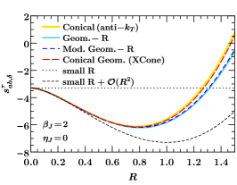
Refer to caption
Refer to caption
Refer to caption
Refer to caption
Refer to caption
Refer to caption
Figure -1372: The coefficient sab,δsubscript𝑠𝑎𝑏𝛿s_{ab,\delta} for the various distance measures and with the small R𝑅R results for beam thrust (left column), C-parameter (middle column) and pTsubscript𝑝𝑇p_{T} (right column) for a jet mass measurement (β=2𝛽2\beta=2) for ηJ=0subscript𝜂𝐽0\eta_{J}=0 (top row) and |ηJ|=1subscript𝜂𝐽1|\eta_{J}|=1 (bottom row) as function of R𝑅R. For the pTsubscript𝑝𝑇p_{T} measurement including the analytic corrections at 𝒪(R2)𝒪superscript𝑅2\mathcal{O}(R^{2}) yield already the exact result for anti-kTsubscript𝑘𝑇k_{T}.
Refer to caption
Refer to caption
Refer to caption
Figure -1371: Same as fig. -1372, but for R=1𝑅1R=1 as function of ηJsubscript𝜂𝐽\eta_{J}.
Refer to caption
Refer to caption
Refer to caption
Figure -1370: The coefficients saJ,Bsubscript𝑠𝑎𝐽𝐵s_{aJ,B} and saJ,Jsubscript𝑠𝑎𝐽𝐽s_{aJ,J} for the various distance measures and with the small R𝑅R results. These are independent of the specific measurements in the beam and jet regions. Shown are saJ,Bsubscript𝑠𝑎𝐽𝐵s_{aJ,B} for ηJ=1,0,1subscript𝜂𝐽101\eta_{J}=-1,0,1 in terms of R𝑅R (left), saJ,Jsubscript𝑠𝑎𝐽𝐽s_{aJ,J} for ηJ=0subscript𝜂𝐽0\eta_{J}=0 as function of R𝑅R (middle) and for R=1𝑅1R=1 as function of ηJsubscript𝜂𝐽\eta_{J} (right).
Refer to caption
Refer to caption
Refer to caption
Refer to caption
Refer to caption
Refer to caption
Refer to caption
Refer to caption
Refer to caption
Figure -1369: The coefficient saJ,δsubscript𝑠𝑎𝐽𝛿s_{aJ,\delta} for the various distance measures and with the small R𝑅R results for beam thrust (left column), C-parameter (middle column) and pTsubscript𝑝𝑇p_{T} (right column) for a jet mass measurement (β=2𝛽2\beta=2) for ηJ=0subscript𝜂𝐽0\eta_{J}=0 (top row), ηJ=1subscript𝜂𝐽1\eta_{J}=1 (middle row) and ηJ=1subscript𝜂𝐽1\eta_{J}=-1 (bottom row) as function of R𝑅R.
Refer to caption
Refer to caption
Refer to caption
Figure -1368: Same as fig. -1369 but for R=1𝑅1R=1 as function of ηJsubscript𝜂𝐽\eta_{J}.
Refer to caption
Refer to caption
Refer to caption
Refer to caption
Figure -1367: The coefficients sab,δsubscript𝑠𝑎𝑏𝛿s_{ab,\delta} (top row) and saJ,δsubscript𝑠𝑎𝐽𝛿s_{aJ,\delta} (bottom row) for a jet angularity with β=1𝛽1\beta=1, for the various distance measures and with the small R𝑅R results for a pTsubscript𝑝𝑇p_{T} jet veto in the beam region, for ηJ=0subscript𝜂𝐽0\eta_{J}=0 in terms of R𝑅R (left column) and for R=1𝑅1R=1 in terms of ηJsubscript𝜂𝐽\eta_{J} (right column).

The contributions from the beam-beam dipole sab,δsubscript𝑠𝑎𝑏𝛿s_{ab,\delta} are shown in fig. -1372 for ηJ=0subscript𝜂𝐽0\eta_{J}=0 and |ηJ|=1subscript𝜂𝐽1|\eta_{J}|=1 as a function of R𝑅R, and in fig. -1371 for R=1𝑅1R=1 as function of ηJsubscript𝜂𝐽\eta_{J}. The results deviate from the 𝒪(R0)𝒪superscript𝑅0\mathcal{O}(R^{0}) result away from R=0𝑅0R=0, in particular also for the phenomenologically relevant values R0.5similar-to𝑅0.5R\sim 0.5. However, including the 𝒪(R2)𝒪superscript𝑅2\mathcal{O}(R^{2}) corrections, the analytic contributions agree very well with the exact results for central rapidities even for values as large as R1similar-to𝑅1R\sim 1. These 𝒪(R2)𝒪superscript𝑅2\mathcal{O}(R^{2}) corrections are the same for all distance measures, which explains why they behave very similar, and they are enhanced by logarithms of the jet radius, as can be seen from eqs. (A.2) and (115). For the transverse momentum beam measurement with a conical anti-kTsubscript𝑘𝑇k_{T} jet (red curves in the right panels of figs. -1372 and -1371), there are in fact no higher order R𝑅R corrections beyond 𝒪(R2)𝒪superscript𝑅2\mathcal{O}(R^{2}) for sab,δsubscript𝑠𝑎𝑏𝛿s_{ab,\delta}. Otherwise, the next corrections are 𝒪(R4)𝒪superscript𝑅4\mathcal{O}(R^{4}) except for the beam thrust case with |ηJ|Rless-than-or-similar-tosubscript𝜂𝐽𝑅|\eta_{J}|\lesssim R where they are 𝒪(R3)𝒪superscript𝑅3\mathcal{O}(R^{3}) due to the kink at η=0𝜂0\eta=0. This explains the larger deviation between the analytic 𝒪(R2)𝒪superscript𝑅2\mathcal{O}(R^{2}) beam thrust result and the exact result for ηJ=0subscript𝜂𝐽0\eta_{J}=0 as seen in the top-left panel of fig. -1372. At large jet rapidities there are sizable differences between the geometric-R measures and the conical (and conical geometric) measure, which is due to the different jet shapes illustrated in fig. -1379.

Results for the beam-jet dipole coefficients saJ,Bsubscript𝑠𝑎𝐽𝐵s_{aJ,B} and saJ,Jsubscript𝑠𝑎𝐽𝐽s_{aJ,J} are shown in fig. -1370 and these coefficients are independent of the measurements in the beam and jet regions. For central rapidities both coefficients differ very little between different distance measures. Away from ηJ=0subscript𝜂𝐽0\eta_{J}=0 there are noticeable differences between the geometric-R, modified geometric-R and conical (anti-kTsubscript𝑘𝑇k_{T} and XCone) measures, as can be seen in the right panel of fig. -1370. In fig. -1369 we plot saJ,δsubscript𝑠𝑎𝐽𝛿s_{aJ,\delta} for ηJ=1,0,1subscript𝜂𝐽101\eta_{J}=-1,0,1 as function of R𝑅R and in fig. -1368 for R=1𝑅1R=1 in terms of ηJsubscript𝜂𝐽\eta_{J}. Once again results are shown for the beam-thrust, C-parameter and pTsubscript𝑝𝑇p_{T}-measurements and β=2𝛽2\beta=2. Compared to the beam-beam dipole, the coefficients are not any more symmetric in ηJηJsubscript𝜂𝐽subscript𝜂𝐽\eta_{J}\leftrightarrow-\eta_{J}. Furthermore, the 𝒪(R2)𝒪superscript𝑅2\mathcal{O}(R^{2}) corrections are not universal for different partitionings, which can lead to sizable deviations for R1similar-to𝑅1R\sim 1, especially for forward jets. This is clearly visible for saJ,Jsubscript𝑠𝑎𝐽𝐽s_{aJ,J}, as shown in the right panel of fig. -1370, or e.g. for saJ,δsubscript𝑠𝑎𝐽𝛿s_{aJ,\delta} with ηJ=1subscript𝜂𝐽1\eta_{J}=1 shown in the middle row of fig. -1369. The analytic results including 𝒪(R2)𝒪superscript𝑅2\mathcal{O}(R^{2}) corrections that are shown correspond to the conical partitioning. The difference with respect to the exact result is very small up to values of R2similar-to𝑅2R\sim 2 for all measurements in the beam region, suggesting that the effective expansion parameter is R/R0𝑅subscript𝑅0R/R_{0} with R02greater-than-or-equivalent-tosubscript𝑅02R_{0}\gtrsim 2. For the geometric-R𝑅R measures the corresponding 𝒪(R2)𝒪superscript𝑅2\mathcal{O}(R^{2}) corrections (not shown) are also close to the full results for R1less-than-or-similar-to𝑅1R\lesssim 1, but deviate much stronger for large values of R𝑅R.

In general, the results for anti-kTsubscript𝑘𝑇k_{T} and XCone jets are almost identical for isolated jets and reasonable values of the jet radius, as expected from the very similar shapes displayed in fig. -1379. This will be different when the distance between jets becomes less than 2R2𝑅2R, as illustrated in fig. -1378. Furthermore, since the shape of isolated anti-kTsubscript𝑘𝑇k_{T} and XCone jets is invariant under boosts along the beam axis, the results for the corresponding soft function coefficients sab,Bsubscript𝑠𝑎𝑏𝐵s_{ab,B}, sab,δsubscript𝑠𝑎𝑏𝛿s_{ab,\delta}, saJ,δsubscript𝑠𝑎𝐽𝛿s_{aJ,\delta}, saJ,Jsubscript𝑠𝑎𝐽𝐽s_{aJ,J} and saJ,δsubscript𝑠𝑎𝐽𝛿s_{aJ,\delta} do not depend on the jet rapidity when using the (boost invariant) pTsubscript𝑝𝑇p_{T}-measurement in the beam region.

For different values of β𝛽\beta the qualitative behavior looks similar. To illustrate this, we display the coefficients sab,δsubscript𝑠𝑎𝑏𝛿s_{ab,\delta} and saJ,δsubscript𝑠𝑎𝐽𝛿s_{aJ,\delta} for β=1𝛽1\beta=1 and the pTsubscript𝑝𝑇p_{T}-measurement in fig. -1367. The most noticeable differences between the distance measures are again between the (modified) Geometric-R and the conical measures away from central rapidity.

5 Conclusions

In this paper we worked out a general setup to calculate one-loop soft functions for exclusive N𝑁N-jet processes at hadron colliders. This method applies to any jet algorithm that satisfies soft-collinear factorization, and for generic infrared- and collinear safe jet measurements and jet vetoes, as long as they reduce to an angularity in the limit where they approach the jet/beam axis. The soft function is calculated using a hemisphere decomposition of the phase space, extending the approach that was used in ref. Jouttenus:2011wh to calculate the N𝑁N-jettiness soft function. The divergences are extracted analytically, such that numerical computations only arise for the finite terms.

We also demonstrated how the method works in practice, providing explicit expressions for single jet production ppL+1 jet𝑝𝑝𝐿1 jetpp\to L+1\text{ jet} for several cases: angularities as jet measurements, beam thrust, C𝐶C-parameter, and transverse momentum as jet vetoes, and anti-kTsubscript𝑘𝑇k_{T} and XCone as jet algorithms. We optimized our method by expanding the finite corrections in the jet radius R𝑅R, obtaining a fully analytical result in the limit R1much-less-than𝑅1R\ll 1. It turns out that the remaining (numerical) contributions are rather small, even for relatively large values of R𝑅R, thus improving the stability.

With the soft functions discussed in this paper, one can calculate resummed cross-section at NNLL or NLL accuracy for exclusive jet processes at the LHC. This same soft function also enters in jet substructure calculations, see e.g. the 2-jettiness calculation of ref. Feige:2012vc , and the subtraction techniques could prove useful for other jet substructure calculations as found in ref. Larkoski:2015kga .

Acknowledgements.
P.P. would like to thank Bahman Dehnadi for pointing out some typos in the draft. This work was supported by the German Science Foundation (DFG) through the Emmy-Noether Grant No. TA 867/1-1, and the Collaborative Research Center (SFB) 676 Particles, Strings and the Early Universe, by the Office of Nuclear Physics of the U.S. Department of Energy under the Grant No. DE-SC0011090, Grant No. DE-AC02-05CH11231, Grant No. DE-AC52-06NA25396, and through the Los Alamos National Lab LDRD Program, by the Simons Foundation through the Investigator grant 327942, by the European Research Council under Grant No. ERC-STG-2015-677323, by the D-ITP consortium, a program of the Netherlands Organization for Scientific Research (NWO) that is funded by the Dutch Ministry of Education, Culture and Science (OCW), and by a Global MISTI Collaboration Grant from MIT. We also thank the Erwin Schrödinger Institute’s program “Challenges and Concepts for Field Theory and Applications in the Era of the LHC Run-2”, where portions of this work were completed.

Appendix A Analytic contributions for ppL+1𝑝𝑝𝐿1pp\to L+1 jet

In this appendix we collect some details about the analytic calculation of several soft function corrections for ppL+1𝑝𝑝𝐿1pp\to L+1 jet discussed in sec. 4. We discuss the jet hemisphere correction to the soft function for angularity measurements in app. A.1, and compute the analytic results for the 𝒪(R2)𝒪superscript𝑅2\mathcal{O}(R^{2}) terms of the soft function coefficients in eq. (4.3) for anti-kTsubscript𝑘𝑇k_{T} in app. A.2.

A.1 Hemisphere soft function correction

We perform the calculation of the jet hemisphere correction for the boost-invariant angularities defined in eq. (59), i.e. Sa<Jsubscript𝑆𝑎𝐽S_{a<J} in eq. (4.2). It is given by the integral

SJ<a({kl},ρ,ηJ)=2(μ2eγE4π)ϵg2ddp(2π)dnanJ(nap)(nJp) 2πδ(p2)θ(p0)FJ<a({km},ρ,ηJ,p),subscript𝑆𝐽𝑎subscript𝑘𝑙𝜌subscript𝜂𝐽2superscriptsuperscript𝜇2superscript𝑒subscript𝛾𝐸4𝜋italic-ϵsuperscript𝑔2superscriptd𝑑𝑝superscript2𝜋𝑑subscript𝑛𝑎subscript𝑛𝐽subscript𝑛𝑎𝑝subscript𝑛𝐽𝑝2𝜋𝛿superscript𝑝2𝜃superscript𝑝0subscript𝐹𝐽𝑎subscript𝑘𝑚𝜌subscript𝜂𝐽𝑝\displaystyle S_{J<a}(\{k_{l}\},\rho,\eta_{J})\!=-2\Bigl{(}\frac{\mu^{2}e^{\gamma_{E}}}{4\pi}\Bigr{)}^{\epsilon}\!g^{2}\!\!\int\!\frac{\mathrm{d}^{d}p}{(2\pi)^{d}}\,\frac{n_{a}\cdot n_{J}}{(n_{a}\cdot p)(n_{J}\cdot p)}\,2\pi\delta(p^{2})\theta(p^{0})\,F_{J<a}(\{k_{m}\},\rho,\eta_{J},p), (94)

with the size of the hemisphere adjusted by the parameter ρ𝜌\rho and the measurement given by

FJ<a({km},ρ,ηJ,p)=δ(kJpTJβ)θ(napnJpρ)δ(kB),subscript𝐹𝐽𝑎subscript𝑘𝑚𝜌subscript𝜂𝐽𝑝𝛿subscript𝑘𝐽subscript𝑝𝑇superscriptsubscript𝐽𝛽𝜃subscript𝑛𝑎𝑝subscript𝑛𝐽𝑝𝜌𝛿subscript𝑘𝐵\displaystyle F_{J<a}(\{k_{m}\},\rho,\eta_{J},p)=\delta\bigl{(}k_{J}-p_{T}\mathcal{R}_{J}^{\beta}\bigr{)}\,\theta\Bigl{(}n_{a}\cdot p-\frac{n_{J}\cdot p}{\rho}\Bigr{)}\,\delta(k_{B})\,, (95)

in analogy to eq. (4.2). Here JsJsubscript𝐽subscript𝑠𝐽\mathcal{R}_{J}\equiv\mathcal{R}_{sJ} denotes the distance of the soft emission with momentum pμsuperscript𝑝𝜇p^{\mu} with respect to the jet direction in azimuth-rapidity space as defined in eq. (2.2). Let us define the momentum projection pksubscript𝑝𝑘p_{k} along a generic light-like direction nksubscript𝑛𝑘n_{k} and the angular distance between two light-like directions s^ijsubscript^𝑠𝑖𝑗\hat{s}_{ij} as

pknkp,s^ijninj2=1cosθij2.\begin{split}p_{k}&\equiv n_{k}\cdot p\,,\qquad\hat{s}_{ij}\equiv\frac{n_{i}\cdot n_{j}}{2}=\frac{1-\cos\theta_{ij}}{2}\,.\end{split} (96)

For any ij𝑖𝑗ij-dipole, the gluon four-momentum can be decomposed as

pμ=pi2s^ijnjμ+pj2s^ijniμ+pijμ,superscript𝑝𝜇subscript𝑝𝑖2subscript^𝑠𝑖𝑗superscriptsubscript𝑛𝑗𝜇subscript𝑝𝑗2subscript^𝑠𝑖𝑗superscriptsubscript𝑛𝑖𝜇superscriptsubscript𝑝subscriptperpendicular-to𝑖𝑗𝜇p^{\mu}=\frac{p_{i}}{2\hat{s}_{ij}}n_{j}^{\mu}+\frac{p_{j}}{2\hat{s}_{ij}}n_{i}^{\mu}+p_{\perp_{ij}}^{\mu}\,, (97)

with the integration measure given by

d42ϵp=pij12ϵ2s^ijdpidpjdpijdΩ22ϵ.superscriptd42italic-ϵ𝑝superscriptsubscript𝑝subscriptperpendicular-to𝑖𝑗12italic-ϵ2subscript^𝑠𝑖𝑗dsubscript𝑝𝑖dsubscript𝑝𝑗dsubscript𝑝subscriptperpendicular-to𝑖𝑗dsubscriptΩ22italic-ϵ\mathrm{d}^{4-2\epsilon}p=\frac{p_{\perp_{ij}}^{1-2\epsilon}}{2\hat{s}_{ij}}\,\mathrm{d}p_{i}\,\mathrm{d}p_{j}\,\mathrm{d}p_{\perp_{ij}}\,\mathrm{d}\Omega_{2-2\epsilon}\,. (98)

The boost-invariant jet angularity can be expressed in this basis, by first writing

pTJβ=(2pjcoshηj)β/2(pT)1β/2,subscript𝑝𝑇superscriptsubscript𝐽𝛽superscript2subscript𝑝𝑗subscript𝜂𝑗𝛽2superscriptsubscript𝑝𝑇1𝛽2\displaystyle p_{T}\mathcal{R}_{J}^{\beta}=(2p_{j}\cosh\eta_{j})^{\beta/2}(p_{T})^{1-\beta/2}, (99)

and then substituting

pT=pij𝒢(q,ϕ)qwithq=pjpij.formulae-sequencesubscript𝑝𝑇subscript𝑝subscriptperpendicular-to𝑖𝑗𝒢𝑞italic-ϕ𝑞with𝑞subscript𝑝𝑗subscript𝑝subscriptperpendicular-to𝑖𝑗\displaystyle p_{T}=\frac{p_{\perp_{ij}}\mathcal{G}(q,\phi)}{q}\quad{\rm with}\,\,q=\frac{p_{j}}{p_{\perp_{ij}}}\,. (100)

The function 𝒢(q,ϕ)𝒢𝑞italic-ϕ\mathcal{G}(q,\phi) is given in general by

𝒢(q,ϕ)=𝒢𝑞italic-ϕabsent\displaystyle\mathcal{G}(q,\phi)= (s^aj+s^ais^ijq22s^ajs^ais^ijqcosϕ)12(s^bj+s^bis^ijq22s^bjs^bis^ijqcos(ϕΔϕij))12.superscriptsubscript^𝑠𝑎𝑗subscript^𝑠𝑎𝑖subscript^𝑠𝑖𝑗superscript𝑞22subscript^𝑠𝑎𝑗subscript^𝑠𝑎𝑖subscript^𝑠𝑖𝑗𝑞italic-ϕ12superscriptsubscript^𝑠𝑏𝑗subscript^𝑠𝑏𝑖subscript^𝑠𝑖𝑗superscript𝑞22subscript^𝑠𝑏𝑗subscript^𝑠𝑏𝑖subscript^𝑠𝑖𝑗𝑞italic-ϕΔsubscriptitalic-ϕ𝑖𝑗12\displaystyle\biggl{(}\hat{s}_{aj}+\frac{\hat{s}_{ai}}{\hat{s}_{ij}}\,q^{2}-2\sqrt{\frac{\hat{s}_{aj}\hat{s}_{ai}}{\hat{s}_{ij}}}\,q\cos\phi\,\biggr{)}^{\frac{1}{2}}\biggl{(}\hat{s}_{bj}+\frac{\hat{s}_{bi}}{\hat{s}_{ij}}\,q^{2}-2\sqrt{\frac{\hat{s}_{bj}\hat{s}_{bi}}{\hat{s}_{ij}}}\,q\cos(\phi-\Delta\phi_{ij})\,\biggr{)}^{\frac{1}{2}}\,. (101)

Here ϕitalic-ϕ\phi is the azimuthal angle in the two-dimensional ijsubscriptperpendicular-to𝑖𝑗\perp_{ij}-space, and ΔϕijΔsubscriptitalic-ϕ𝑖𝑗\Delta\phi_{ij} is the difference in azimuth (with respect to the beam axis) between the dipole directions i𝑖i and j𝑗j. Thus the jet angularity can be written as

pTJβ=pijqβ1[𝒢(q,ϕ)]1β/2(2coshηJ)β/2.subscript𝑝𝑇superscriptsubscript𝐽𝛽subscript𝑝subscriptperpendicular-to𝑖𝑗superscript𝑞𝛽1superscriptdelimited-[]𝒢𝑞italic-ϕ1𝛽2superscript2subscript𝜂𝐽𝛽2p_{T}\mathcal{R}_{J}^{\beta}=p_{\perp_{ij}}\,q^{\beta-1}\,[\mathcal{G}(q,\phi)]^{1-\beta/2}\,(2\cosh\eta_{J})^{\beta/2}\,. (102)

Let us specialize to the case i=a𝑖𝑎i=a and j=J𝑗𝐽j=J. The hemisphere phase space is given by

Hemisphere J<a:θ(q0q),q0=ρs^aJ,Hemisphere J<a:𝜃subscript𝑞0𝑞subscript𝑞0𝜌subscript^𝑠𝑎𝐽\displaystyle\text{Hemisphere $J<a$:}\quad\theta(q_{0}-q),\quad q_{0}=\sqrt{\rho\,\hat{s}_{aJ}}\,, (103)

with s^aJ=eηJ/(2coshηJ)subscript^𝑠𝑎𝐽superscript𝑒subscript𝜂𝐽2subscript𝜂𝐽\hat{s}_{aJ}=e^{-\eta_{J}}/(2\cosh\eta_{J}). For the case β>1𝛽1\beta>1, dimensional regularization regulates all the divergences. Using the basis of eq. (97), after the trivial integrations and changing variable from pJsubscript𝑝𝐽p_{J} to q𝑞q, eq. (94) reads

SJ<a({kl},ρ,ηJ)subscript𝑆𝐽𝑎subscript𝑘𝑙𝜌subscript𝜂𝐽\displaystyle S_{J<a}(\{k_{l}\},\rho,\eta_{J}) =2g2(2π)32ϵ(μ2eγE4π)ϵ(2coshηJ)βϵkJ1+2ϵδ(kB)absent2superscript𝑔2superscript2𝜋32italic-ϵsuperscriptsuperscript𝜇2superscript𝑒subscript𝛾𝐸4𝜋italic-ϵsuperscript2subscript𝜂𝐽𝛽italic-ϵsuperscriptsubscript𝑘𝐽12italic-ϵ𝛿subscript𝑘𝐵\displaystyle=-\frac{2g^{2}}{(2\pi)^{3-2\epsilon}}\Bigl{(}\frac{\mu^{2}e^{\gamma_{E}}}{4\pi}\Bigr{)}^{\epsilon}\,\frac{(2\cosh\eta_{J})^{\beta\epsilon}}{k_{J}^{1+2\epsilon}}\,\delta(k_{B})
×dΩ22ϵ0q0dqq12ϵ(β1)[𝒢(q,ϕ)]ϵ(2β).\displaystyle\quad\times\int\mathrm{d}\Omega_{2-2\epsilon}\int_{0}^{q_{0}}\frac{\mathrm{d}q\,}{q^{1-2\epsilon(\beta-1)}}\bigl{[}\mathcal{G}(q,\phi)\bigr{]}^{\epsilon(2-\beta)}\,. (104)

Performing the integrals and expanding in ϵitalic-ϵ\epsilon,

SJ<a({kl},ρ,ηJ)subscript𝑆𝐽𝑎subscript𝑘𝑙𝜌subscript𝜂𝐽\displaystyle S_{J<a}(\{k_{l}\},\rho,\eta_{J}) =αs4πδ(kB)β1[8μrβ11(kJμrβ1)4ϵ1μrβ10(kJμrβ1)\displaystyle=\frac{\alpha_{s}}{4\pi}\,\frac{\delta(k_{B})}{\beta-1}\biggl{[}\frac{8}{\mu\,r^{\beta-1}}\,\mathcal{L}_{1}\biggl{(}\frac{k_{J}}{\mu\,r^{\beta-1}}\biggr{)}-\frac{4}{\epsilon}\frac{1}{\mu\,r^{\beta-1}}\,\mathcal{L}_{0}\biggl{(}\frac{k_{J}}{\mu\,r^{\beta-1}}\biggr{)}
+δ(kJ)(2ϵ2π262(β1)(β2))+𝒪(ϵ)],\displaystyle\quad+\delta(k_{J})\biggl{(}\frac{2}{\epsilon^{2}}-\frac{\pi^{2}}{6}-2(\beta-1)(\beta-2)\,\mathcal{I}\biggr{)}+\mathcal{O}(\epsilon)\biggr{]}\,, (105)

where r=(2coshηJeηJρ)1/2𝑟superscript2subscript𝜂𝐽superscript𝑒subscript𝜂𝐽𝜌12r=(2\cosh\eta_{J}\,e^{-\eta_{J}}\rho)^{1/2} and

=1πππdϕ0q0dqqln[2coshηJ𝒢(q,ϕ)]=θ(r1)ln2r.1𝜋superscriptsubscript𝜋𝜋differential-ditalic-ϕsuperscriptsubscript0subscript𝑞0d𝑞𝑞2subscript𝜂𝐽𝒢𝑞italic-ϕ𝜃𝑟1superscript2𝑟\displaystyle\mathcal{I}=\frac{1}{\pi}\int_{-\pi}^{\pi}\mathrm{d}\phi\int_{0}^{q_{0}}\frac{\mathrm{d}q}{q}\ln\left[2\cosh\eta_{J}\,\mathcal{G}(q,\phi)\right]=\theta(r-1)\ln^{2}r\,. (106)

Setting ρ=ρRJ(R,ηJ)𝜌superscriptsubscript𝜌𝑅𝐽𝑅subscript𝜂𝐽\rho=\rho_{R}^{J}(R,\eta_{J}) as defined in eq. (69) yields r=R𝑟𝑅r=R and thus the result in eq. (76). For the case β=1𝛽1\beta=1, one can see from eq. (A.1) that an additional rapidity regulator is needed as q0𝑞0q\to 0, which can be chosen to be (ν/2p0)ηsuperscript𝜈2superscript𝑝0𝜂(\nu/2p^{0})^{\eta}, as discussed below eq. (3). Following a similar procedure, one obtains the result of eq. (4.2).

Alternatively, one can get the hemisphere soft function for boost-invariant angularities by adding the finite correction in eq. (3) to eqs. (42) and (3), which correspond to the standard angularities in e+esuperscript𝑒superscript𝑒e^{+}e^{-}-collisions defined in eq. (37). Using the same variables defined above, one gets

4I1,J<a4subscript𝐼1𝐽𝑎\displaystyle 4I_{1,J<a} =2(β2)πππdϕ0q0dqqln[2coshηJ𝒢(q,ϕ)1+e2ηJq22eηJqcosϕ]absent2𝛽2𝜋superscriptsubscript𝜋𝜋differential-ditalic-ϕsuperscriptsubscript0subscript𝑞0d𝑞𝑞2subscript𝜂𝐽𝒢𝑞italic-ϕ1superscript𝑒2subscript𝜂𝐽superscript𝑞22superscript𝑒subscript𝜂𝐽𝑞italic-ϕ\displaystyle=-\frac{2(\beta-2)}{\pi}\int_{-\pi}^{\pi}\mathrm{d}\phi\int_{0}^{q_{0}}\frac{\mathrm{d}q}{q}\ln\left[\frac{2\cosh\eta_{J}\,\mathcal{G}(q,\phi)}{1+e^{2\eta_{J}}q^{2}-2e^{\eta_{J}}q\cos\phi}\right]
=2(β2)[θ(R1)ln2R2θ(ReηJ2coshηJ1)ln2(ReηJ2coshηJ)].absent2𝛽2delimited-[]𝜃𝑅1superscript2𝑅2𝜃𝑅superscript𝑒subscript𝜂𝐽2subscript𝜂𝐽1superscript2𝑅superscript𝑒subscript𝜂𝐽2subscript𝜂𝐽\displaystyle=-2(\beta-2)\biggl{[}\theta(R-1)\ln^{2}R-2\,\theta\Bigl{(}\frac{R\,e^{\eta_{J}}}{2\cosh\eta_{J}}-1\Bigr{)}\ln^{2}\Bigl{(}\frac{R\,e^{\eta_{J}}}{2\cosh\eta_{J}}\Bigr{)}\biggr{]}\,. (107)

By adding this correction to eqs. (42) and (3), with cJ=(2coshηJ)β1subscript𝑐𝐽superscript2subscript𝜂𝐽𝛽1c_{J}=(2\cosh\eta_{J})^{\beta-1}, one recovers again the results in eqs. (76) and (4.2).

A.2 Corrections at 𝒪(R2)𝒪superscript𝑅2\mathcal{O}(R^{2})

Here we outline the analytic calculation of the soft function corrections in eq. (4.3) at 𝒪(R2)𝒪superscript𝑅2\mathcal{O}(R^{2}) in the small jet radius expansion. A similar computation has been performed in ref. Liu:2014oog for a jet mass measurement in dijet processes close to the kinematic threshold. We give the results for a conical (anti-kTsubscript𝑘𝑇k_{T}) jet with the measurement of arbitrary jet angularities and general smooth jet vetoes (including in addition the beam thrust case).

First, we consider the contributions from the beam-beam dipole. Here the 𝒪(R2)𝒪superscript𝑅2\mathcal{O}(R^{2}) corrections are the leading contributions that account for the jet region. Since the deviations between the jet boundaries for different partitionings are in addition power suppressed by the jet radius all sets of distance measures discussed in sec. 2 lead to the same result at 𝒪(R2)𝒪superscript𝑅2\mathcal{O}(R^{2}). The term sab,Bsubscript𝑠𝑎𝑏𝐵s_{ab,B} in eq. (4.3) corresponds to the jet area giving sab,B=4R2subscript𝑠𝑎𝑏𝐵4superscript𝑅2s_{ab,B}=4R^{2}. The coefficient sab,δsubscript𝑠𝑎𝑏𝛿s_{ab,\delta} is given by the integral in eq. (4.2), which yields at 𝒪(R2)𝒪superscript𝑅2\mathcal{O}(R^{2})

sab,δsubscript𝑠𝑎𝑏𝛿\displaystyle s_{ab,\delta} =4πdΔηππdϕ(β2ln[(Δη)2+ϕ2]lnfB(ηJ))θ(R2(Δη)2ϕ2)+𝒪(R4)absent4𝜋superscriptsubscriptdifferential-dΔ𝜂superscriptsubscript𝜋𝜋differential-ditalic-ϕ𝛽2superscriptΔ𝜂2superscriptitalic-ϕ2subscript𝑓𝐵subscript𝜂𝐽𝜃superscript𝑅2superscriptΔ𝜂2superscriptitalic-ϕ2𝒪superscript𝑅4\displaystyle=\frac{4}{\pi}\int_{-\infty}^{\infty}\mathrm{d}\Delta\eta\int_{-\pi}^{\pi}\mathrm{d}\phi\,\Bigl{(}\frac{\beta}{2}\ln\bigl{[}(\Delta\eta)^{2}+\phi^{2}\bigr{]}-\ln f_{B}(\eta_{J})\Bigr{)}\,\theta\Bigl{(}R^{2}-(\Delta\eta)^{2}-\phi^{2}\Bigr{)}+\mathcal{O}(R^{4})
=2R2[β(2lnR1)2lnfB(ηJ)]+𝒪(R4).absent2superscript𝑅2delimited-[]𝛽2𝑅12subscript𝑓𝐵subscript𝜂𝐽𝒪superscript𝑅4\displaystyle=2R^{2}\Bigl{[}\beta\bigl{(}2\ln R-1\bigr{)}-2\ln f_{B}(\eta_{J})\Bigr{]}+\mathcal{O}(R^{4})\,. (108)

In fact, for conical jets and a transverse momentum veto, i.e. fB(η)=1subscript𝑓𝐵𝜂1f_{B}(\eta)=1, any higher order corrections in R𝑅R vanish, so that eq. (A.2) provides already the exact one-loop result for this case.

Next, we discuss the contributions from the beam-jet dipole, which in general differ for different partitionings. The corrections for real radiation inside the jet region can be written as

SaJ(J)=αs2πeγEϵμ2ϵπΓ(12ϵ)1kJ1+2ϵ[IaJ,R1(J)+(IaJ(J)IaJ,R1(J))=ΔIaJ(J)],superscriptsubscript𝑆𝑎𝐽𝐽subscript𝛼𝑠2𝜋superscript𝑒subscript𝛾𝐸italic-ϵsuperscript𝜇2italic-ϵ𝜋Γ12italic-ϵ1superscriptsubscript𝑘𝐽12italic-ϵdelimited-[]superscriptsubscript𝐼much-less-than𝑎𝐽𝑅1𝐽subscriptsuperscriptsubscript𝐼𝑎𝐽𝐽superscriptsubscript𝐼much-less-than𝑎𝐽𝑅1𝐽absentΔsuperscriptsubscript𝐼𝑎𝐽𝐽\displaystyle S_{aJ}^{(J)}=-\frac{\alpha_{s}}{2\pi}\,e^{\gamma_{E}\epsilon}\mu^{2\epsilon}\frac{\sqrt{\pi}}{\Gamma(\frac{1}{2}-\epsilon)}\,\frac{1}{k_{J}^{1+2\epsilon}}\,\Bigl{[}I_{aJ,R\ll 1}^{(J)}+\underbrace{(I_{aJ}^{(J)}-I_{aJ,R\ll 1}^{(J)})}_{=\Delta I_{aJ}^{(J)}}\Bigr{]}\,, (109)

where IaJ,R1(J)superscriptsubscript𝐼much-less-than𝑎𝐽𝑅1𝐽I_{aJ,R\ll 1}^{(J)} denotes the leading small-R result at 𝒪(1)𝒪1\mathcal{O}(1) and ΔIaJ(J)Δsuperscriptsubscript𝐼𝑎𝐽𝐽\Delta I_{aJ}^{(J)} contains all corrections which are suppressed by the jet size. The latter term can be expanded in ϵitalic-ϵ\epsilon and is given up to 𝒪(ϵ)𝒪italic-ϵ\mathcal{O}(\epsilon) by

ΔIaJ(J)Δsuperscriptsubscript𝐼𝑎𝐽𝐽\displaystyle\Delta I_{aJ}^{(J)} =1πdΔηππdϕθ[dB(ηJ+Δη)dJ(ηJ+Δη,ϕ,R)]absent1𝜋superscriptsubscriptdifferential-dΔ𝜂superscriptsubscript𝜋𝜋differential-ditalic-ϕ𝜃delimited-[]subscript𝑑𝐵subscript𝜂𝐽Δ𝜂subscript𝑑𝐽subscript𝜂𝐽Δ𝜂italic-ϕ𝑅\displaystyle=\frac{1}{\pi}\int_{-\infty}^{\infty}\mathrm{d}\Delta\eta\int_{-\pi}^{\pi}\mathrm{d}\phi\,\,\theta\bigl{[}d_{B}(\eta_{J}+\Delta\eta)-d_{J}(\eta_{J}+\Delta\eta,\phi,R)\bigr{]} (110)
×[(eΔηcoshΔηcosϕ2(Δη)2+ϕ2)\displaystyle\quad\times\biggl{[}\biggl{(}\frac{e^{\Delta\eta}}{\cosh\Delta\eta-\cos\phi}-\frac{2}{(\Delta\eta)^{2}+\phi^{2}}\biggr{)}
+2ϵ(eΔη(β2ln[2coshΔη2cosϕ]ln|sinϕ|)coshΔηcosϕβln[(Δη)2+ϕ2]2ln|ϕ|(Δη)2+ϕ2)].\displaystyle\qquad+2\epsilon\biggl{(}\frac{e^{\Delta\eta}\bigl{(}\frac{\beta}{2}\ln\bigl{[}2\cosh\Delta\eta-2\cos\phi\bigr{]}-\ln\lvert\sin\phi\rvert\bigr{)}}{\cosh\Delta\eta-\cos\phi}-\frac{\beta\ln\bigl{[}(\Delta\eta)^{2}+\phi^{2}\bigr{]}-2\ln\lvert\phi\rvert}{(\Delta\eta)^{2}+\phi^{2}}\biggr{)}\biggr{]}\,.

Expanding the integrand in R𝑅R yields for conical jets

ΔIaJ(J,kT)|𝒪(R2)=R2[12+ϵ(76β2+(β1)lnR+ln2)].evaluated-atΔsuperscriptsubscript𝐼𝑎𝐽𝐽subscript𝑘𝑇𝒪superscript𝑅2superscript𝑅2delimited-[]12italic-ϵ76𝛽2𝛽1𝑅2\displaystyle\Delta I_{aJ}^{(J,k_{T})}\Bigr{|}_{\mathcal{O}(R^{2})}=R^{2}\biggl{[}\frac{1}{2}+\epsilon\biggl{(}\frac{7}{6}-\frac{\beta}{2}+(\beta-1)\ln R+\ln 2\biggr{)}\biggr{]}\,. (111)

The corrections for real radiation inside the beam region can be similarly written as

SaJ(B)=αs2πeγEϵμ2ϵπΓ(12ϵ)1kB1+2ϵ[IaJ,R1(B)+(IaJ(B)IaJ,R1(B))=ΔIaJ(B)].superscriptsubscript𝑆𝑎𝐽𝐵subscript𝛼𝑠2𝜋superscript𝑒subscript𝛾𝐸italic-ϵsuperscript𝜇2italic-ϵ𝜋Γ12italic-ϵ1superscriptsubscript𝑘𝐵12italic-ϵdelimited-[]superscriptsubscript𝐼much-less-than𝑎𝐽𝑅1𝐵subscriptsuperscriptsubscript𝐼𝑎𝐽𝐵superscriptsubscript𝐼much-less-than𝑎𝐽𝑅1𝐵absentΔsuperscriptsubscript𝐼𝑎𝐽𝐵\displaystyle S_{aJ}^{(B)}=-\frac{\alpha_{s}}{2\pi}\,e^{\gamma_{E}\epsilon}\mu^{2\epsilon}\frac{\sqrt{\pi}}{\Gamma(\frac{1}{2}-\epsilon)}\,\frac{1}{k_{B}^{1+2\epsilon}}\,\Bigl{[}I_{aJ,R\ll 1}^{(B)}+\underbrace{(I_{aJ}^{(B)}-I_{aJ,R\ll 1}^{(B)})}_{=\Delta I_{aJ}^{(B)}}\Bigr{]}\,. (112)

Here ΔIaJ(B)Δsuperscriptsubscript𝐼𝑎𝐽𝐵\Delta I_{aJ}^{(B)} acts as a subtractive contribution inside the jet region and is given by

ΔIaJ(B)Δsuperscriptsubscript𝐼𝑎𝐽𝐵\displaystyle\Delta I_{aJ}^{(B)} =1πdΔηππdϕθ[dB(ηJ+Δη)dJ(ηJ+Δη,ϕ,R)]absent1𝜋superscriptsubscriptdifferential-dΔ𝜂superscriptsubscript𝜋𝜋differential-ditalic-ϕ𝜃delimited-[]subscript𝑑𝐵subscript𝜂𝐽Δ𝜂subscript𝑑𝐽subscript𝜂𝐽Δ𝜂italic-ϕ𝑅\displaystyle=-\frac{1}{\pi}\int_{-\infty}^{\infty}\mathrm{d}\Delta\eta\int_{-\pi}^{\pi}\mathrm{d}\phi\,\,\theta\bigl{[}d_{B}(\eta_{J}+\Delta\eta)-d_{J}(\eta_{J}+\Delta\eta,\phi,R)\bigr{]}
×[(eΔηcoshΔηcosϕ2(Δη)2+ϕ2)\displaystyle\quad\times\biggl{[}\biggl{(}\frac{e^{\Delta\eta}}{\cosh\Delta\eta-\cos\phi}-\frac{2}{(\Delta\eta)^{2}+\phi^{2}}\biggr{)}
+2ϵ(eΔη(lnfB(η)ln|sinϕ|)coshΔηcosϕ2(lnfB(ηJ)ln|ϕ|)(Δη)2+ϕ2)].\displaystyle\qquad+2\epsilon\biggl{(}\frac{e^{\Delta\eta}(\ln f_{B}(\eta)-\ln\lvert\sin\phi\rvert)}{\cosh\Delta\eta-\cos\phi}-\frac{2(\ln f_{B}(\eta_{J})-\ln\lvert\phi\rvert)}{(\Delta\eta)^{2}+\phi^{2}}\biggr{)}\biggr{]}\,. (113)

Expanding the integrand in R𝑅R yields for conical jets and a smooth function fB(η)subscript𝑓𝐵𝜂f_{B}(\eta)

ΔIaJ(B,kT)=R2[12+ϵ(76lnR+lnfB(ηJ)+2fB(ηJ)+fB′′(ηJ)fB(ηJ)(fB(ηJ)fB(ηJ))2+ln2)].Δsuperscriptsubscript𝐼𝑎𝐽𝐵subscript𝑘𝑇superscript𝑅2delimited-[]12italic-ϵ76𝑅subscript𝑓𝐵subscript𝜂𝐽2superscriptsubscript𝑓𝐵subscript𝜂𝐽superscriptsubscript𝑓𝐵′′subscript𝜂𝐽subscript𝑓𝐵subscript𝜂𝐽superscriptsuperscriptsubscript𝑓𝐵subscript𝜂𝐽subscript𝑓𝐵subscript𝜂𝐽22\displaystyle\Delta I_{aJ}^{(B,k_{T})}=-R^{2}\biggl{[}\frac{1}{2}+\epsilon\biggl{(}\frac{7}{6}-\ln R+\ln f_{B}(\eta_{J})+\frac{2f_{B}^{\prime}(\eta_{J})+f_{B}^{\prime\prime}(\eta_{J})}{f_{B}(\eta_{J})}-\Bigl{(}\frac{f_{B}^{\prime}(\eta_{J})}{f_{B}(\eta_{J})}\Bigr{)}^{2}+\ln 2\biggr{)}\biggr{]}\,. (114)

Using eqs. (109), (111), (112) and (114) the soft function coefficients at 𝒪(R2)𝒪superscript𝑅2\mathcal{O}(R^{2}) for the beam-jet dipole contributions read for anti-kTsubscript𝑘𝑇k_{T} jets

saJ,J(kT)|𝒪(R2)evaluated-atsubscriptsuperscript𝑠subscript𝑘𝑇𝑎𝐽𝐽𝒪superscript𝑅2\displaystyle s^{(k_{T})}_{aJ,J}\Bigr{|}_{\mathcal{O}(R^{2})} =saJ,B(kT)|𝒪(R2)=R2,absentevaluated-atsubscriptsuperscript𝑠subscript𝑘𝑇𝑎𝐽𝐵𝒪superscript𝑅2superscript𝑅2\displaystyle=-s^{(k_{T})}_{aJ,B}\Bigr{|}_{\mathcal{O}(R^{2})}=-R^{2}\,,
saJ,δ(kT)|𝒪(R2)evaluated-atsubscriptsuperscript𝑠subscript𝑘𝑇𝑎𝐽𝛿𝒪superscript𝑅2\displaystyle s^{(k_{T})}_{aJ,\delta}\Bigr{|}_{\mathcal{O}(R^{2})} =R2[βlnRβ2lnfB(ηJ)2fB(ηJ)+fB′′(ηJ)fB(ηJ)+(fB(ηJ)fB(ηJ))2].absentsuperscript𝑅2delimited-[]𝛽𝑅𝛽2subscript𝑓𝐵subscript𝜂𝐽2superscriptsubscript𝑓𝐵subscript𝜂𝐽superscriptsubscript𝑓𝐵′′subscript𝜂𝐽subscript𝑓𝐵subscript𝜂𝐽superscriptsuperscriptsubscript𝑓𝐵subscript𝜂𝐽subscript𝑓𝐵subscript𝜂𝐽2\displaystyle=R^{2}\biggl{[}\beta\ln R-\frac{\beta}{2}-\ln f_{B}(\eta_{J})-\frac{2f_{B}^{\prime}(\eta_{J})+f_{B}^{\prime\prime}(\eta_{J})}{f_{B}(\eta_{J})}+\Bigl{(}\frac{f_{B}^{\prime}(\eta_{J})}{f_{B}(\eta_{J})}\Bigr{)}^{2}\biggr{]}\,. (115)

Since the beam thrust veto has a kink at η=0𝜂0\eta=0, eq. (115) does not fully determine all power suppressed terms up to 𝒪(R2)𝒪superscript𝑅2\mathcal{O}(R^{2}) if |ηJ|<Rsubscript𝜂𝐽𝑅|\eta_{J}|<R. In this case the next-to leading correction is of 𝒪(R)𝒪𝑅\mathcal{O}(R) and the additional contribution with respect to eq. (115) reads

ΔsaJ,δ(kT)Δsubscriptsuperscript𝑠subscript𝑘𝑇𝑎𝐽𝛿\displaystyle\Delta s^{(k_{T})}_{aJ,\delta} =θ(1|x|){16Rπ[1x2+|x|(ln(2|x|)1)arccos|x||x|2Cl2(arccos(12x2))]\displaystyle=\theta(1-|x|)\biggl{\{}\frac{16R}{\pi}\biggl{[}\sqrt{1-x^{2}}+\lvert x\rvert(\ln(2\lvert x\rvert)-1)\arccos\lvert x\rvert-\frac{\lvert x\rvert}{2}\,{\rm Cl}_{2}\Bigl{(}\arccos(1-2x^{2})\Bigr{)}\biggr{]}
+4R2π[π2(θ(x)θ(x))+3x1x2+arcsin(x)2x|x|arccos|x|)]+𝒪(R3)},\displaystyle\quad+\frac{4R^{2}}{\pi}\biggl{[}\frac{\pi}{2}\bigl{(}\theta(-x)-\theta(x)\bigr{)}+3x\sqrt{1-x^{2}}+\arcsin(x)-2x\lvert x\rvert\arccos\lvert x\rvert\Bigr{)}\biggr{]}+\mathcal{O}(R^{3})\biggr{\}}\,, (116)

where xηJ/R𝑥subscript𝜂𝐽𝑅x\equiv\eta_{J}/R and the Cl2(θ)Im[Li2(eiθ)]subscriptCl2𝜃Imdelimited-[]subscriptLi2superscript𝑒𝑖𝜃{\rm Cl}_{2}(\theta)\equiv{\rm Im}[\textrm{Li}_{2}(e^{i\theta})].

Results for jet regions from a different partitioning can be obtained by considering deviations from the circular jet shape in addition. For the conical geometric distance measure in eq. (16) corresponding to a XCone default jet the results at 𝒪(R2)𝒪superscript𝑅2\mathcal{O}(R^{2}) are the same as for the conical measure (i.e. for an anti-kTsubscript𝑘𝑇k_{T} jet).

Appendix B Numerical evaluation of soft function integrations

We discuss the numerical evaluation of the boundary mismatch integrals IaJBsuperscriptsubscript𝐼𝑎𝐽𝐵I_{aJ}^{B} and IaJJsuperscriptsubscript𝐼𝑎𝐽𝐽I_{aJ}^{J} in eq. (83) for ppL+1𝑝𝑝𝐿1pp\to L+1 jet. To compute them efficiently we need to determine the integration bounds. These depend on the relations between the distance measures dB(p)subscript𝑑𝐵𝑝d_{B}(p) and dJ(p)subscript𝑑𝐽𝑝d_{J}(p) and between the projections napsubscript𝑛𝑎𝑝n_{a}\cdot p and nJp/ρJsubscript𝑛𝐽𝑝subscript𝜌𝐽n_{J}\cdot p/\rho_{J} used for the analytic calculation of the hemisphere results. We discuss here the explicit boundaries only for the most important case, the conical (anti-kTsubscript𝑘𝑇k_{T}) measure. For the geometric measures (including the conical geometric XCone measure) one can follow a strategy similar to Jouttenus:2011wh using coordinates based on the lightcone projections napsubscript𝑛𝑎𝑝n_{a}\cdot p and nJpsubscript𝑛𝐽𝑝n_{J}\cdot p. Furthermore, we also explain why the integrals encoding the corrections to the small R𝑅R limit give only a moderate numerical impact, even for sizable values of the jet radius.

B.1 Integration bounds for the conical measure
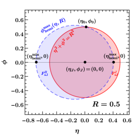
Refer to caption
Refer to caption
Refer to caption
Figure -1366: Illustration of the phase space misalignment between the hemisphere jet region with ρJ=ρJRsubscript𝜌𝐽superscriptsubscript𝜌𝐽𝑅\rho_{J}=\rho_{J}^{R} (blue, dashed) and a conical jet area (red, solid) for ηJ=0subscript𝜂𝐽0\eta_{J}=0 and R=0.5,1.0,1.5𝑅0.51.01.5R=0.5,1.0,1.5. The areas which do not overlap correspond to the integration domains of the integrals IaJBsuperscriptsubscript𝐼𝑎𝐽𝐵I_{aJ}^{B} and IaJJsuperscriptsubscript𝐼𝑎𝐽𝐽I_{aJ}^{J}, respectively.

For the conical measure the integration boundaries can be most easily obtained in beam coordinates η𝜂\eta, ϕitalic-ϕ\phi. The conditions from the measurement functions in eq. (4.2) read

FaJB::subscriptsuperscript𝐹𝐵𝑎𝐽absent\displaystyle F^{B}_{aJ}:\quad R2<(Δη)2+ϕ2andρJeηJcoshηJ<eΔη(coshΔηcosϕ),formulae-sequencesuperscript𝑅2superscriptΔ𝜂2superscriptitalic-ϕ2andsubscript𝜌𝐽superscript𝑒subscript𝜂𝐽subscript𝜂𝐽superscript𝑒Δ𝜂Δ𝜂italic-ϕ\displaystyle R^{2}<(\Delta\eta)^{2}+\phi^{2}\quad{\rm and}\quad\rho_{J}e^{-\eta_{J}}\cosh\eta_{J}<e^{\Delta\eta}(\cosh\Delta\eta-\cos\phi)\,,
FaJJ::subscriptsuperscript𝐹𝐽𝑎𝐽absent\displaystyle F^{J}_{aJ}:\quad R2>(Δη)2+ϕ2andρJeηJcoshηJ>eΔη(coshΔηcosϕ).formulae-sequencesuperscript𝑅2superscriptΔ𝜂2superscriptitalic-ϕ2andsubscript𝜌𝐽superscript𝑒subscript𝜂𝐽subscript𝜂𝐽superscript𝑒Δ𝜂Δ𝜂italic-ϕ\displaystyle R^{2}>(\Delta\eta)^{2}+\phi^{2}\quad{\rm and}\quad\rho_{J}e^{-\eta_{J}}\cosh\eta_{J}>e^{\Delta\eta}(\cosh\Delta\eta-\cos\phi)\,. (117)

We use the value ρJ=ρJRsubscript𝜌𝐽superscriptsubscript𝜌𝐽𝑅\rho_{J}=\rho_{J}^{R} in eq. (69), which eliminates the dependence on the jet rapidity ηJsubscript𝜂𝐽\eta_{J} (in favor of the jet radius R𝑅R) in the second relation and leads to integrals which are power suppressed in R𝑅R. (The computation for arbitrary ρJsubscript𝜌𝐽\rho_{J} can be carried out similarly.) The associated hemisphere mismatch regions are displayed in fig. -1366. For FaJJsubscriptsuperscript𝐹𝐽𝑎𝐽F^{J}_{aJ} the integration boundaries read

dΔηππdϕθ(R2(Δη)2ϕ2)θ(nJpρJRnap)superscriptsubscriptdifferential-dΔ𝜂superscriptsubscript𝜋𝜋differential-ditalic-ϕ𝜃superscript𝑅2superscriptΔ𝜂2superscriptitalic-ϕ2𝜃subscript𝑛𝐽𝑝subscriptsuperscript𝜌𝑅𝐽subscript𝑛𝑎𝑝\displaystyle\int_{-\infty}^{\infty}\mathrm{d}\Delta\eta\int_{-\pi}^{\pi}\mathrm{d}\phi\,\theta\bigl{(}R^{2}-(\Delta\eta)^{2}-\phi^{2}\bigr{)}\,\theta\Bigl{(}\frac{n_{J}\cdot p}{\rho^{R}_{J}}-n_{a}\cdot p\Bigr{)}
=η0(R)ηhemimax(R)dΔηϕhemimax(Δη,R)R2(Δη)2dϕ+ηhemimax(R)RdΔη0R2(Δη)2dϕ+(ϕϕ),\displaystyle\quad=\int_{\eta_{0}(R)}^{\eta^{\rm max}_{\rm hemi}(R)}\mathrm{d}\Delta\eta\int_{\phi^{\rm max}_{\rm hemi}(\Delta\eta,R)}^{\sqrt{R^{2}-(\Delta\eta)^{2}}}\mathrm{d}\phi+\int_{\eta^{\rm max}_{\rm hemi}(R)}^{R}\mathrm{d}\Delta\eta\int_{0}^{\sqrt{R^{2}-(\Delta\eta)^{2}}}\mathrm{d}\phi+(\phi\leftrightarrow-\phi)\,, (118)

where we have defined

ϕhemimax(Δη,R)=arccos(eΔη+(1R2)eΔη2),ηhemimax(R)=ln(1+R),formulae-sequencesubscriptsuperscriptitalic-ϕmaxhemiΔ𝜂𝑅superscript𝑒Δ𝜂1superscript𝑅2superscript𝑒Δ𝜂2subscriptsuperscript𝜂maxhemi𝑅1𝑅\displaystyle\phi^{\rm max}_{\rm hemi}(\Delta\eta,R)=\arccos\biggl{(}\frac{e^{\Delta\eta}+(1-R^{2})e^{-\Delta\eta}}{2}\biggr{)},\quad\eta^{\rm max}_{\rm hemi}(R)=\ln(1+R), (119)

and η0(R)subscript𝜂0𝑅\eta_{0}(R) is the solution of the transcendental equation

[η0(R)]2+[ϕhemimax(η0(R),R)]2=R2.superscriptdelimited-[]subscript𝜂0𝑅2superscriptdelimited-[]subscriptsuperscriptitalic-ϕmaxhemisubscript𝜂0𝑅𝑅2superscript𝑅2\displaystyle[\eta_{0}(R)]^{2}+\bigl{[}\phi^{\rm max}_{\rm hemi}(\eta_{0}(R),R)\bigr{]}^{2}=R^{2}\,. (120)

For FaJBsubscriptsuperscript𝐹𝐵𝑎𝐽F^{B}_{aJ} we get

dΔηππdϕθ((Δη)2+ϕ2R2)θ(napnJpρJR)superscriptsubscriptdifferential-dΔ𝜂superscriptsubscript𝜋𝜋differential-ditalic-ϕ𝜃superscriptΔ𝜂2superscriptitalic-ϕ2superscript𝑅2𝜃subscript𝑛𝑎𝑝subscript𝑛𝐽𝑝subscriptsuperscript𝜌𝑅𝐽\displaystyle\int_{-\infty}^{\infty}\mathrm{d}\Delta\eta\int_{-\pi}^{\pi}\mathrm{d}\phi\,\theta\bigl{(}(\Delta\eta)^{2}+\phi^{2}-R^{2}\bigr{)}\,\theta\Bigl{(}n_{a}\cdot p-\frac{n_{J}\cdot p}{\rho^{R}_{J}}\Bigr{)}
=θ(R1)[ηhemimin(R)RdΔη0ϕhemimax(Δη,R)dϕ+Rη0(R)dΔηR2(Δη)2ϕhemimax(Δη,R)dϕ]absent𝜃𝑅1delimited-[]superscriptsubscriptsubscriptsuperscript𝜂minhemi𝑅𝑅differential-dΔ𝜂superscriptsubscript0subscriptsuperscriptitalic-ϕmaxhemiΔ𝜂𝑅differential-ditalic-ϕsuperscriptsubscript𝑅subscript𝜂0𝑅differential-dΔ𝜂superscriptsubscriptsuperscript𝑅2superscriptΔ𝜂2subscriptsuperscriptitalic-ϕmaxhemiΔ𝜂𝑅differential-ditalic-ϕ\displaystyle=\theta(R\leq 1)\biggl{[}\int_{\eta^{\rm min}_{\rm hemi}(R)}^{-R}\!\mathrm{d}\Delta\eta\int_{0}^{\phi^{\rm max}_{\rm hemi}(\Delta\eta,R)}\!\mathrm{d}\phi+\int_{-R}^{\eta_{0}(R)}\!\mathrm{d}\Delta\eta\int_{\sqrt{R^{2}-(\Delta\eta)^{2}}}^{\phi^{\rm max}_{\rm hemi}(\Delta\eta,R)}\mathrm{d}\phi\biggr{]}
+θ(Rπ>R>1)[ηπ(R)dΔη0πdϕ+ηπ(R)RdΔη0ϕhemimax(Δη,R)dϕ+Rη0(R)dΔηR2(Δη)2ϕhemimax(Δη,R)dϕ]𝜃subscript𝑅𝜋𝑅1delimited-[]superscriptsubscriptsubscript𝜂𝜋𝑅differential-dΔ𝜂superscriptsubscript0𝜋differential-ditalic-ϕsuperscriptsubscriptsubscript𝜂𝜋𝑅𝑅differential-dΔ𝜂superscriptsubscript0subscriptsuperscriptitalic-ϕmaxhemiΔ𝜂𝑅differential-ditalic-ϕsuperscriptsubscript𝑅subscript𝜂0𝑅differential-dΔ𝜂superscriptsubscriptsuperscript𝑅2superscriptΔ𝜂2subscriptsuperscriptitalic-ϕmaxhemiΔ𝜂𝑅differential-ditalic-ϕ\displaystyle+\theta(R_{\pi}\!>\!R\!>\!1)\biggl{[}\int_{-\infty}^{\eta_{\pi}(R)}\!\!\!\!\!\!\!\mathrm{d}\Delta\eta\int_{0}^{\pi}\!\!\mathrm{d}\phi+\int_{\eta_{\pi}(R)}^{-R}\!\!\mathrm{d}\Delta\eta\int_{0}^{\phi^{\rm max}_{\rm hemi}(\Delta\eta,R)}\!\!\!\!\!\mathrm{d}\phi+\!\int_{-R}^{\eta_{0}(R)}\!\!\mathrm{d}\Delta\eta\int_{\sqrt{R^{2}-(\Delta\eta)^{2}}}^{\phi^{\rm max}_{\rm hemi}(\Delta\eta,R)}\!\mathrm{d}\phi\biggr{]}
+θ(RRπ)[RdΔη0πdϕ+Rηπ(R)dΔηR2(Δη)2πdϕ+ηπ(R)η0(R)dΔηR2(Δη)2ϕhemimax(Δη,R)dϕ]𝜃𝑅subscript𝑅𝜋delimited-[]superscriptsubscript𝑅differential-dΔ𝜂superscriptsubscript0𝜋differential-ditalic-ϕsubscriptsuperscriptsubscript𝜂𝜋𝑅𝑅differential-dΔ𝜂superscriptsubscriptsuperscript𝑅2superscriptΔ𝜂2𝜋differential-ditalic-ϕsuperscriptsubscriptsubscript𝜂𝜋𝑅subscript𝜂0𝑅differential-dΔ𝜂superscriptsubscriptsuperscript𝑅2superscriptΔ𝜂2subscriptsuperscriptitalic-ϕmaxhemiΔ𝜂𝑅differential-ditalic-ϕ\displaystyle+\theta(R\geq R_{\pi})\biggl{[}\int_{-\infty}^{-R}\!\!\mathrm{d}\Delta\eta\int_{0}^{\pi}\!\mathrm{d}\phi+\int^{\eta_{\pi}(R)}_{-R}\!\mathrm{d}\Delta\eta\int_{\sqrt{R^{2}-(\Delta\eta)^{2}}}^{\pi}\mathrm{d}\phi+\int_{\eta_{\pi}(R)}^{\eta_{0}(R)}\!\!\!\!\mathrm{d}\Delta\eta\int_{\sqrt{R^{2}-(\Delta\eta)^{2}}}^{\phi^{\rm max}_{\rm hemi}(\Delta\eta,R)}\!\mathrm{d}\phi\biggr{]}
+(ϕϕ),\displaystyle+(\phi\leftrightarrow-\phi)\,, (121)

where we have defined

ηhemimin(R)=ln(1R),ηπ(R)subscriptsuperscript𝜂minhemi𝑅1𝑅subscript𝜂𝜋𝑅\displaystyle\eta^{\rm min}_{\rm hemi}(R)=\ln(1-R),\quad\eta_{\pi}(R) =ln(R1),absent𝑅1\displaystyle=\ln(R-1), (122)

and Rπ1.28subscript𝑅𝜋1.28R_{\pi}\approx 1.28 is the solution of the transcendental equation

ηπ(Rπ)=Rπ.subscript𝜂𝜋subscript𝑅𝜋subscript𝑅𝜋\displaystyle\eta_{\pi}(R_{\pi})=-R_{\pi}\,. (123)

With these explicit limits the integrals can be evaluated efficiently.

B.2 Power suppression of boundary integrals

We have seen in fig. -1366 that for a small jet radius the jet region from the hemisphere decomposition with ρJRsubscriptsuperscript𝜌𝑅𝐽\rho^{R}_{J} and the actual conical partitioning largely overlap giving small results for the non-hemisphere corrections. However, for R1similar-to𝑅1R\sim 1 the areas in the η𝜂\eta-ϕitalic-ϕ\phi plane begin to differ very significantly, which might suggest that the associated corrections become very large in this regime and the results for the small R𝑅R-expansion do not provide a good approximation. As we have seen in sec. 4.4 this turns out not to be the case since the deviations of the jet areas in the beam coordinates are not representative for the size of the associated corrections. Instead it is more meaningful to compare the jet areas in the boosted frame where the jet and beam direction are back-to-back and soft radiation from the beam-jet dipole aJ𝑎𝐽aJ is uniform in the respective rapidity-azimuth coordinates η~~𝜂\tilde{\eta}, ϕ~~italic-ϕ\tilde{\phi}. The associated transformation rules between the sets of coordinates are explicitly given in ref. Kasemets:2015uus . In fig. -1365 we display the jet regions in these coordinates for the conical measure (red) and for the hemisphere decomposition with ρJ=ρJRsubscript𝜌𝐽superscriptsubscript𝜌𝐽𝑅\rho_{J}=\rho_{J}^{R} for different values of R𝑅R. The areas which do not overlap correspond directly to the integrals I0,aJBsuperscriptsubscript𝐼0𝑎𝐽𝐵I_{0,aJ}^{B} and I0,aJJsuperscriptsubscript𝐼0𝑎𝐽𝐽I_{0,aJ}^{J}, respectively, while I1,aJBsuperscriptsubscript𝐼1𝑎𝐽𝐵I_{1,aJ}^{B} and I1,aJJsuperscriptsubscript𝐼1𝑎𝐽𝐽I_{1,aJ}^{J} are (logarithmic) moments in these regions. These are individually of 𝒪(R)similar-toabsent𝒪𝑅\sim\mathcal{O}(R), which can be also confirmed by an analytic expansion indicated by the black, dotted line. In total the contributions from FaJBsuperscriptsubscript𝐹𝑎𝐽𝐵F_{aJ}^{B} and FaJJsuperscriptsubscript𝐹𝑎𝐽𝐽F_{aJ}^{J} cancel each other at this order leading to a net contribution to the soft function of 𝒪(R2)𝒪superscript𝑅2\mathcal{O}(R^{2}).111111For the corrections saJ,Bsubscript𝑠𝑎𝐽𝐵s_{aJ,B} and saJ,Jsubscript𝑠𝑎𝐽𝐽s_{aJ,J} in eq. (4.3) this is obvious since only the difference between the two mismatch areas in fig. -1365 enters. For the correction saJ,δsubscript𝑠𝑎𝐽𝛿s_{aJ,\delta} this holds for measurements which are continuous functions in η𝜂\eta, ϕitalic-ϕ\phi due to the fact that at leading order in R𝑅R the integrands are constant in these areas.
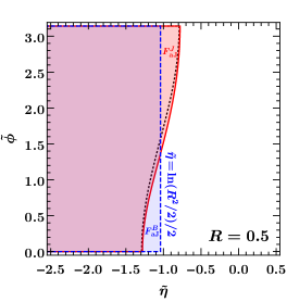
Refer to caption
Refer to caption
Refer to caption
Figure -1365: Illustration of the phase space misalignment between the hemisphere jet region with ρJ=ρJRsubscript𝜌𝐽superscriptsubscript𝜌𝐽𝑅\rho_{J}=\rho_{J}^{R} (blue, dashed) and a conical partitioning (red, solid) for ηJ=0subscript𝜂𝐽0\eta_{J}=0 and R=0.5,1.0,1.5𝑅0.51.01.5R=0.5,1.0,1.5 in the boosted frame where the jet and beam a𝑎a are back-to-back. The areas which do not overlap scale as the integrals IaJBsuperscriptsubscript𝐼𝑎𝐽𝐵I_{aJ}^{B} and IaJJsuperscriptsubscript𝐼𝑎𝐽𝐽I_{aJ}^{J}, respectively. The black dotted lines indicates the analytic result for the conical measure at 𝒪(R)𝒪𝑅\mathcal{O}(R). The associated corrections to the coefficients saJ,Jsubscript𝑠𝑎𝐽𝐽s_{aJ,J}, saJ,Bsubscript𝑠𝑎𝐽𝐵s_{aJ,B} correspond to the areas between the dashed and solid curves.

Appendix C Analytic corrections for pp𝑝𝑝absentpp\to dijets

Beyond single jet production, pp𝑝𝑝absentpp\to dijets is another process of phenomenological relevance for measurements like jet mass. The full computation of the associated soft function corrections for arbitrary jet and beam measurements and partitionings can be carried out following the hemisphere decompositions discussed in secs. 3 and 4. Here we compute the analytic corrections for pp𝑝𝑝absentpp\to dijets (j1,j2subscript𝑗1subscript𝑗2j_{1},j_{2}) in a small R𝑅R expansion up to terms at 𝒪(R2)𝒪superscript𝑅2\mathcal{O}(R^{2}), whereas the full R𝑅R dependence can be determined numerically but now including a jet-jet dipole. For definiteness and simplicity we consider conical jets with a jet mass measurement (i.e. angularity in defined in eq. (59) with β=2𝛽2\beta=2) and a pTsubscript𝑝𝑇p_{T} jet veto. For generic R<π/2𝑅𝜋2R<\pi/2 we can write the renormalized one-loop soft function as121212For R<π/2𝑅𝜋2R<\pi/2 (i.e. as long as the jet regions do not share a common boundary) the measurements and partitioning are invariant under boosts along the beam axis, such that this correction mainly depends on the relative rapidity of the jets Δη12Δsubscript𝜂12\Delta\eta_{12} and the jet radius. Since the rapidity regularization breaks boost invariance, there is, however, also a residual dependence on the individual jet rapidities appearing in sa1,Bsubscript𝑠𝑎1𝐵s_{a1,B}.

S^2κ(1)({ki},R,η1,η2,μ,ν)=αs(μ)4π{𝐓a𝐓b[16μ(1(kBμ)0(kBμ)ln(νμ))δ(k1)δ(k2)\displaystyle\widehat{S}^{\kappa(1)}_{2}(\{k_{i}\},R,\eta_{1},\eta_{2},\mu,\nu)=\frac{\alpha_{s}(\mu)}{4\pi}\biggl{\{}{\bf T}_{a}\cdot{\bf T}_{b}\biggl{[}\frac{16}{\mu}\Bigl{(}{\mathcal{L}}_{1}\Bigl{(}\frac{k_{B}}{\mu}\Bigr{)}-{\mathcal{L}}_{0}\Bigl{(}\frac{k_{B}}{\mu}\Bigr{)}\ln\Bigl{(}\frac{\nu}{\mu}\Bigr{)}\Bigr{)}\,\delta(k_{1})\,\delta(k_{2})
+sab,B(R)(2μ0(kBμ)δ(k1)δ(k2)1μ0(k1μ)δ(kB)δ(k2)1μ0(k2μ)δ(kB)δ(k1))subscript𝑠𝑎𝑏𝐵𝑅2𝜇subscript0subscript𝑘𝐵𝜇𝛿subscript𝑘1𝛿subscript𝑘21𝜇subscript0subscript𝑘1𝜇𝛿subscript𝑘𝐵𝛿subscript𝑘21𝜇subscript0subscript𝑘2𝜇𝛿subscript𝑘𝐵𝛿subscript𝑘1\displaystyle\quad+s_{ab,B}(R)\Bigl{(}\frac{2}{\mu}\,{\mathcal{L}}_{0}\Bigl{(}\frac{k_{B}}{\mu}\Bigr{)}\,\delta(k_{1})\,\delta(k_{2})-\frac{1}{\mu}\,{\mathcal{L}}_{0}\Bigl{(}\frac{k_{1}}{\mu}\Bigr{)}\,\delta(k_{B})\,\delta(k_{2})-\frac{1}{\mu}\,{\mathcal{L}}_{0}\Bigl{(}\frac{k_{2}}{\mu}\Bigr{)}\,\delta(k_{B})\,\delta(k_{1})\Bigr{)}
+sab,δ(R)δ(kB)δ(k1)δ(k2)]+𝐓1𝐓2[8μ1(k1μ)δ(k2)δ(kB)+8μ1(k2μ)δ(k1)δ(kB)\displaystyle\quad+s_{ab,\delta}(R)\,\delta(k_{B})\,\delta(k_{1})\,\delta(k_{2})\biggr{]}+{\bf T}_{1}\cdot{\bf T}_{2}\biggl{[}\frac{8}{\mu}\,{\mathcal{L}}_{1}\Bigl{(}\frac{k_{1}}{\mu}\Bigr{)}\,\delta(k_{2})\,\delta(k_{B})+\frac{8}{\mu}\,{\mathcal{L}}_{1}\Bigl{(}\frac{k_{2}}{\mu}\Bigr{)}\,\delta(k_{1})\,\delta(k_{B})
+s12,J(R,Δη12)(1μ0(k1μ)δ(k2)+1μ0(k2μ)δ(k1))δ(kB)subscript𝑠12𝐽𝑅Δsubscript𝜂121𝜇subscript0subscript𝑘1𝜇𝛿subscript𝑘21𝜇subscript0subscript𝑘2𝜇𝛿subscript𝑘1𝛿subscript𝑘𝐵\displaystyle\quad+s_{12,J}(R,\Delta\eta_{12})\Bigl{(}\frac{1}{\mu}\,{\mathcal{L}}_{0}\Bigl{(}\frac{k_{1}}{\mu}\Bigr{)}\,\delta(k_{2})+\frac{1}{\mu}\,{\mathcal{L}}_{0}\Bigl{(}\frac{k_{2}}{\mu}\Bigr{)}\,\delta(k_{1})\Bigr{)}\delta(k_{B})
+s12,B(R,Δη12)1μ0(kBμ)δ(k1)δ(k2)+s12,δ(R,Δη12)δ(k1)δ(k2)δ(kB)]\displaystyle\quad+s_{12,B}(R,\Delta\eta_{12})\,\frac{1}{\mu}\,{\mathcal{L}}_{0}\Bigl{(}\frac{k_{B}}{\mu}\Bigr{)}\,\delta(k_{1})\,\delta(k_{2})+s_{12,\delta}(R,\Delta\eta_{12})\,\delta(k_{1})\,\delta(k_{2})\,\delta(k_{B})\biggr{]}
+𝐓a𝐓1[8μ1(k1μ)δ(kB)δ(k2)+8μ1(kBμ)δ(k1)δ(k2)8μ0(kBμ)ln(νμ)δ(k1)δ(k2)\displaystyle\quad+{\bf T}_{a}\cdot{\bf T}_{1}\biggl{[}\frac{8}{\mu}\,{\mathcal{L}}_{1}\Bigl{(}\frac{k_{1}}{\mu}\Bigr{)}\,\delta(k_{B})\,\delta(k_{2})+\frac{8}{\mu}\,{\mathcal{L}}_{1}\Bigl{(}\frac{k_{B}}{\mu}\Bigr{)}\,\delta(k_{1})\,\delta(k_{2})-\frac{8}{\mu}\,\mathcal{L}_{0}\Bigl{(}\frac{k_{B}}{\mu}\Bigr{)}\ln\Bigl{(}\frac{\nu}{\mu}\Bigr{)}\,\delta(k_{1})\,\delta(k_{2})
+sa1,1(R)1μ0(k1μ)δ(kB)δ(k2)+sa1,2(R,Δη12)1μ0(k2μ)δ(kB)δ(k1)subscript𝑠𝑎11𝑅1𝜇subscript0subscript𝑘1𝜇𝛿subscript𝑘𝐵𝛿subscript𝑘2subscript𝑠𝑎12𝑅Δsubscript𝜂121𝜇subscript0subscript𝑘2𝜇𝛿subscript𝑘𝐵𝛿subscript𝑘1\displaystyle\quad+s_{a1,1}(R)\,\frac{1}{\mu}\,{\mathcal{L}}_{0}\Bigl{(}\frac{k_{1}}{\mu}\Bigr{)}\,\delta(k_{B})\,\delta(k_{2})+s_{a1,2}(R,\Delta\eta_{12})\,\frac{1}{\mu}\,{\mathcal{L}}_{0}\Bigl{(}\frac{k_{2}}{\mu}\Bigr{)}\,\delta(k_{B})\,\delta(k_{1})
+sa1,B(R,η1,Δη12)1μ0(kBμ)δ(k1)δ(k2)+sa1,δ(R,Δη12)δ(kB)δ(k1)δ(k2)]\displaystyle\quad+s_{a1,B}(R,\eta_{1},\Delta\eta_{12})\,\frac{1}{\mu}\,{\mathcal{L}}_{0}\Bigl{(}\frac{k_{B}}{\mu}\Bigr{)}\,\delta(k_{1})\,\delta(k_{2})+s_{a1,\delta}(R,\Delta\eta_{12})\,\delta(k_{B})\,\delta(k_{1})\,\delta(k_{2})\biggr{]}
+𝐓b𝐓1[Δη12Δη12]+𝐓b𝐓2[(k1,k2,η1)(k2,k1,η2)]subscript𝐓𝑏subscript𝐓1delimited-[]Δsubscript𝜂12Δsubscript𝜂12subscript𝐓𝑏subscript𝐓2delimited-[]subscript𝑘1subscript𝑘2subscript𝜂1subscript𝑘2subscript𝑘1subscript𝜂2\displaystyle\quad+{\bf T}_{b}\cdot{\bf T}_{1}\biggl{[}\Delta\eta_{12}\to-\Delta\eta_{12}\biggr{]}+{\bf T}_{b}\cdot{\bf T}_{2}\biggl{[}(k_{1},k_{2},\eta_{1})\to(k_{2},k_{1},\eta_{2})\biggr{]}
+𝐓a𝐓2[(k1,k2,η1,Δη12)(k2,k1,η2,Δη12)]},\displaystyle\quad+{\bf T}_{a}\cdot{\bf T}_{2}\biggl{[}(k_{1},k_{2},\eta_{1},\Delta\eta_{12})\to(k_{2},k_{1},\eta_{2},-\Delta\eta_{12})\biggr{]}\biggr{\}}\,, (124)

where Δη12η1η2Δsubscript𝜂12subscript𝜂1subscript𝜂2\Delta\eta_{12}\equiv\eta_{1}-\eta_{2} is the difference between the rapidities of the two jets and R1=R2R<π/2subscript𝑅1subscript𝑅2𝑅𝜋2R_{1}=R_{2}\equiv R<\pi/2. The replacements in the last line are always with respect to the terms with the color factor 𝐓a𝐓1subscript𝐓𝑎subscript𝐓1{\bf T}_{a}\cdot{\bf T}_{1}.

The contributions from the beam-beam dipole are equivalent to the case of single production given in eq. (4.3) and app. A.2, i.e.

sab,B(R)=4R2+𝒪(R4),sab,δ(R)=π23+4R2(2lnR1)+𝒪(R4).formulae-sequencesubscript𝑠𝑎𝑏𝐵𝑅4superscript𝑅2𝒪superscript𝑅4subscript𝑠𝑎𝑏𝛿𝑅superscript𝜋234superscript𝑅22𝑅1𝒪superscript𝑅4\displaystyle s_{ab,B}(R)=4R^{2}+\mathcal{O}(R^{4})\,,\quad s_{ab,\delta}(R)=-\frac{\pi^{2}}{3}+4R^{2}(2\ln R-1)+\mathcal{O}(R^{4})\,. (125)

The contributions from the beam-jet dipoles are also closely related to the ones for single production given in eq. (4.3) and app. A.2 with the difference that starting at 𝒪(R2)𝒪superscript𝑅2\mathcal{O}(R^{2}) there is now also a correction due to emissions into the phase space region of the second jet, which concerns the coefficients sa1,2subscript𝑠𝑎12s_{a1,2}, sa1,Bsubscript𝑠𝑎1𝐵s_{a1,B} and sa1,δsubscript𝑠𝑎1𝛿s_{a1,\delta} and can be easily computed analytically in analogy to app. A.2. We get

sa1,1(R)subscript𝑠𝑎11𝑅\displaystyle s_{a1,1}(R) =8lnRR2+𝒪(R4),absent8𝑅superscript𝑅2𝒪superscript𝑅4\displaystyle=-8\ln R-R^{2}+\mathcal{O}(R^{4})\,, (126)
sa1,2(R,Δη12)subscript𝑠𝑎12𝑅Δsubscript𝜂12\displaystyle s_{a1,2}(R,\Delta\eta_{12}) =R2eΔη12cosh2(Δη122)+𝒪(R4),absentsuperscript𝑅2superscript𝑒Δsubscript𝜂12superscript2Δsubscript𝜂122𝒪superscript𝑅4\displaystyle=-R^{2}\frac{e^{-\Delta\eta_{12}}}{\cosh^{2}\Bigl{(}\frac{\Delta\eta_{12}}{2}\Bigr{)}}+\mathcal{O}(R^{4})\,,
sa1,B(R,η,Δη12)subscript𝑠𝑎1𝐵𝑅𝜂Δsubscript𝜂12\displaystyle s_{a1,B}(R,\eta,\Delta\eta_{12}) =8lnR+8η+R2[1+eΔη12cosh2(Δη122)]+𝒪(R4),absent8𝑅8𝜂superscript𝑅2delimited-[]1superscript𝑒Δsubscript𝜂12superscript2Δsubscript𝜂122𝒪superscript𝑅4\displaystyle=8\ln R+8\eta+R^{2}\biggl{[}1+\frac{e^{-\Delta\eta_{12}}}{\cosh^{2}\Bigl{(}\frac{\Delta\eta_{12}}{2}\Bigr{)}}\biggr{]}+\mathcal{O}(R^{4})\,,
sa1,δ(R,Δη12)subscript𝑠𝑎1𝛿𝑅Δsubscript𝜂12\displaystyle s_{a1,\delta}(R,\Delta\eta_{12}) =4ln2R(2θ(R1))+R2(2lnR1)[1+eΔη12cosh2(Δη122)]+𝒪(R4).absent4superscript2𝑅2𝜃𝑅1superscript𝑅22𝑅1delimited-[]1superscript𝑒Δsubscript𝜂12superscript2Δsubscript𝜂122𝒪superscript𝑅4\displaystyle=4\ln^{2}R(2-\theta(R-1))+R^{2}(2\ln R-1)\biggl{[}1+\frac{e^{-\Delta\eta_{12}}}{\cosh^{2}\Bigl{(}\frac{\Delta\eta_{12}}{2}\Bigr{)}}\biggr{]}+\mathcal{O}(R^{4})\,.

We demonstrate in fig. -1364 that including the terms up to 𝒪(R2)𝒪superscript𝑅2\mathcal{O}(R^{2}) gives a very good approximation of the full results, even for R1similar-to𝑅1R\sim 1.

Refer to caption
Refer to caption
Refer to caption
Refer to caption
Figure -1364: The full coefficients sa1,2subscript𝑠𝑎12s_{a1,2} (top) and sa1,δsubscript𝑠𝑎1𝛿s_{a1,\delta} (bottom) together with the small R𝑅R for conical (anti-kTsubscript𝑘𝑇k_{T}) jets for a jet mass measurement (β=2𝛽2\beta=2) and a pTsubscript𝑝𝑇p_{T} veto, for Δη12=1Δsubscript𝜂121\Delta\eta_{12}=1 in terms of R𝑅R (left) and for R=1𝑅1R=1 in terms of Δη12Δsubscript𝜂12\Delta\eta_{12} (right).

The only remaining ingredient is the correction from the jet-jet dipole. The leading small-R𝑅R results have been computed in ref. Hornig:2016ahz , which we have reproduced.131313Reference Hornig:2016ahz considers a pTsubscript𝑝𝑇p_{T}-veto with a rapidity cutoff ηcutsubscript𝜂cut\eta_{\rm cut}. For the jet-jet dipole the effect due to ηcutsubscript𝜂cut\eta_{\rm cut} is power suppressed in 1/eηcut1superscript𝑒subscript𝜂cut1/e^{\eta_{\rm cut}}, while for the other dipole contributions it leads to different results than those given above. The 𝒪(R2)𝒪superscript𝑅2\mathcal{O}(R^{2}) corrections can be computed following app. A.2. This gives

s12,J(R,Δη12)subscript𝑠12𝐽𝑅Δsubscript𝜂12\displaystyle s_{12,J}(R,\Delta\eta_{12}) =8lnRR2tanh2Δη122+𝒪(R4),absent8𝑅superscript𝑅2superscript2Δsubscript𝜂122𝒪superscript𝑅4\displaystyle=-8\ln R-R^{2}\tanh^{2}\frac{\Delta\eta_{12}}{2}+\mathcal{O}(R^{4})\,, (127)
s12,B(R,Δη12)subscript𝑠12𝐵𝑅Δsubscript𝜂12\displaystyle s_{12,B}(R,\Delta\eta_{12}) =16ln(2coshΔη122)2s12,J(Δη12,R),absent162Δsubscript𝜂1222subscript𝑠12𝐽Δsubscript𝜂12𝑅\displaystyle=-16\ln\Bigl{(}2\cosh\frac{\Delta\eta_{12}}{2}\Bigr{)}-2s_{12,J}(\Delta\eta_{12},R)\,,
s12,δ(R,Δη12)subscript𝑠12𝛿𝑅Δsubscript𝜂12\displaystyle s_{12,\delta}(R,\Delta\eta_{12}) =16ln2R8ln2(2coshΔη122)+2(Δη12)2π23absent16superscript2𝑅8superscript22Δsubscript𝜂1222superscriptΔsubscript𝜂122superscript𝜋23\displaystyle=16\ln^{2}R-8\ln^{2}\Bigl{(}2\cosh\frac{\Delta\eta_{12}}{2}\Bigr{)}+2(\Delta\eta_{12})^{2}-\frac{\pi^{2}}{3}
+R2[2(2lnR1)tanh2Δη122]+𝒪(R4).superscript𝑅2delimited-[]22𝑅1superscript2Δsubscript𝜂122𝒪superscript𝑅4\displaystyle\quad+R^{2}\Bigl{[}2(2\ln R-1)\tanh^{2}\frac{\Delta\eta_{12}}{2}\biggr{]}+\mathcal{O}(R^{4})\,.

In fig. -1363 we compare the full numeric results for these coefficients to the analytic expressions. Again the small R𝑅R expansion provides an excellent approximation of the full result for the jet-jet dipole contribution. Together with the findings for the beam-beam and beam-jet dipole corrections this indicates that keeping terms up to 𝒪(R2)𝒪superscript𝑅2\mathcal{O}(R^{2}) is likely sufficient for phenomenological purposes.
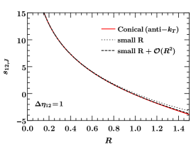
Refer to caption
Refer to caption
Refer to caption
Refer to caption
Figure -1363: The full coefficients s12,Bsubscript𝑠12𝐵s_{12,B} (top) and s12,δsubscript𝑠12𝛿s_{12,\delta} (bottom) together with the small R𝑅R results for conical (anti-kTsubscript𝑘𝑇k_{T}) jets for a jet mass measurement (β=2𝛽2\beta=2) and a pTsubscript𝑝𝑇p_{T} veto, for Δη12=1Δsubscript𝜂121\Delta\eta_{12}=1 in terms of R𝑅R (left) and for R=1𝑅1R=1 in terms of Δη12Δsubscript𝜂12\Delta\eta_{12} (right).

We remark that for jet vetoes which are not boost invariant, all of the dipoles, in particular also the jet-jet dipole, depend on the individual jet rapidities. For multijet processes or an additional recoiling color singlet state the soft function depends in addition on the separation of the jets in azimuth. The analytic computation for these cases is significantly more involved.

References

  • (1) T. T. Jouttenus, I. W. Stewart, F. J. Tackmann, and W. J. Waalewijn, The Soft Function for Exclusive N-Jet Production at Hadron Colliders, Phys.Rev. D83 (2011) 114030, [arXiv:1102.4344].
  • (2) C. W. Bauer, S. Fleming, and M. E. Luke, Summing Sudakov logarithms in BXsγ𝐵subscript𝑋𝑠𝛾B\to X_{s}\gamma in effective field theory, Phys. Rev. D63 (2000) 014006, [hep-ph/0005275].
  • (3) C. W. Bauer, S. Fleming, D. Pirjol, and I. W. Stewart, An Effective field theory for collinear and soft gluons: Heavy to light decays, Phys. Rev. D63 (2001) 114020, [hep-ph/0011336].
  • (4) C. W. Bauer and I. W. Stewart, Invariant operators in collinear effective theory, Phys.Lett. B516 (2001) 134–142, [hep-ph/0107001].
  • (5) C. W. Bauer, D. Pirjol, and I. W. Stewart, Soft collinear factorization in effective field theory, Phys. Rev. D65 (2002) 054022, [hep-ph/0109045].
  • (6) C. W. Bauer and A. V. Manohar, Shape function effects in BXsγ𝐵subscript𝑋𝑠𝛾B\to X_{s}\gamma and BXuν¯𝐵subscript𝑋𝑢¯𝜈B\to X_{u}\ell\bar{\nu} decays, Phys. Rev. D70 (2004) 034024, [hep-ph/0312109].
  • (7) S. Fleming, A. K. Leibovich, and T. Mehen, Resumming the color octet contribution to e+eJ/ψsuperscript𝑒superscript𝑒𝐽𝜓e^{+}e^{-}\to J/\psi + X𝑋X, Phys. Rev. D68 (2003) 094011, [hep-ph/0306139].
  • (8) T. Becher and M. Neubert, Toward a NNLO calculation of the B¯Xsγ¯𝐵subscript𝑋𝑠𝛾\bar{B}\to X_{s}\gamma decay rate with a cut on photon energy. II. Two-loop result for the jet function, Phys. Lett. B637 (2006) 251–259, [hep-ph/0603140].
  • (9) T. Becher and M. D. Schwartz, Direct photon production with effective field theory, JHEP 1002 (2010) 040, [arXiv:0911.0681].
  • (10) T. Becher and G. Bell, The gluon jet function at two-loop order, Phys. Lett. B695 (2011) 252–258, [arXiv:1008.1936].
  • (11) A. J. Larkoski, D. Neill, and J. Thaler, Jet Shapes with the Broadening Axis, JHEP 1404 (2014) 017, [arXiv:1401.2158].
  • (12) I. W. Stewart, F. J. Tackmann, and W. J. Waalewijn, The Quark Beam Function at NNLL, JHEP 09 (2010) 005, [arXiv:1002.2213].
  • (13) C. F. Berger, C. Marcantonini, I. W. Stewart, F. J. Tackmann, and W. J. Waalewijn, Higgs Production with a Central Jet Veto at NNLL+NNLO, JHEP 04 (2011) 092, [arXiv:1012.4480].
  • (14) T. Becher and M. Neubert, Drell-Yan Production at Small qTsubscript𝑞𝑇q_{T}, Transverse Parton Distributions and the Collinear Anomaly, Eur.Phys.J. C71 (2011) 1665, [arXiv:1007.4005].
  • (15) T. Becher and M. Neubert, Factorization and NNLL Resummation for Higgs Production with a Jet Veto, JHEP 1207 (2012) 108, [arXiv:1205.3806].
  • (16) J.-Y. Chiu, A. Jain, D. Neill, and I. Z. Rothstein, A Formalism for the Systematic Treatment of Rapidity Logarithms in Quantum Field Theory, JHEP 1205 (2012) 084, [arXiv:1202.0814].
  • (17) T. Gehrmann, T. Luebbert, and L. L. Yang, Calculation of the transverse parton distribution functions at next-to-next-to-leading order, JHEP 06 (2014) 155, [arXiv:1403.6451].
  • (18) J. R. Gaunt, M. Stahlhofen, and F. J. Tackmann, The Quark Beam Function at Two Loops, JHEP 04 (2014) 113, [arXiv:1401.5478].
  • (19) J. Gaunt, M. Stahlhofen, and F. J. Tackmann, The Gluon Beam Function at Two Loops, JHEP 08 (2014) 020, [arXiv:1405.1044].
  • (20) T. Lübbert, J. Oredsson, and M. Stahlhofen, Rapidity renormalized TMD soft and beam functions at two loops, JHEP 03 (2016) 168, [arXiv:1602.01829].
  • (21) I. Moult, I. W. Stewart, F. J. Tackmann, and W. J. Waalewijn, Employing Helicity Amplitudes for Resummation, Phys. Rev. D93 (2016), no. 9 094003, [arXiv:1508.02397].
  • (22) I. W. Stewart, F. J. Tackmann, and W. J. Waalewijn, N-Jettiness: An Inclusive Event Shape to Veto Jets, Phys. Rev. Lett. 105 (2010) 092002, [arXiv:1004.2489].
  • (23) I. W. Stewart, F. J. Tackmann, and W. J. Waalewijn, Factorization at the LHC: From PDFs to Initial State Jets, Phys. Rev. D81 (2010) 094035, [arXiv:0910.0467].
  • (24) J. Thaler and K. Van Tilburg, Maximizing Boosted Top Identification by Minimizing N-subjettiness, JHEP 02 (2012) 093, [arXiv:1108.2701].
  • (25) T. T. Jouttenus, I. W. Stewart, F. J. Tackmann, and W. J. Waalewijn, Jet mass spectra in Higgs boson plus one jet at next-to-next-to-leading logarithmic order, Phys.Rev. D88 (2013), no. 5 054031, [arXiv:1302.0846].
  • (26) J. Thaler and K. Van Tilburg, Identifying Boosted Objects with N-subjettiness, JHEP 1103 (2011) 015, [arXiv:1011.2268].
  • (27) I. W. Stewart, F. J. Tackmann, J. Thaler, C. K. Vermilion, and T. F. Wilkason, XCone: N-jettiness as an Exclusive Cone Jet Algorithm, JHEP 11 (2015) 072, [arXiv:1508.01516].
  • (28) M. Cacciari, G. P. Salam, and G. Soyez, The Anti-k(t) jet clustering algorithm, JHEP 04 (2008) 063, [arXiv:0802.1189].
  • (29) J. Thaler and T. F. Wilkason, Resolving Boosted Jets with XCone, JHEP 12 (2015) 051, [arXiv:1508.01518].
  • (30) J. R. Walsh and S. Zuberi, Factorization Constraints on Jet Substructure, arXiv:1110.5333.
  • (31) J.-y. Chiu, A. Jain, D. Neill, and I. Z. Rothstein, The Rapidity Renormalization Group, Phys.Rev.Lett. 108 (2012) 151601, [arXiv:1104.0881].
  • (32) J. R. Gaunt, Glauber Gluons and Multiple Parton Interactions, JHEP 07 (2014) 110, [arXiv:1405.2080].
  • (33) M. Zeng, Drell-Yan process with jet vetoes: breaking of generalized factorization, JHEP 10 (2015) 189, [arXiv:1507.01652].
  • (34) I. Z. Rothstein and I. W. Stewart, An Effective Field Theory for Forward Scattering and Factorization Violation, arXiv:1601.04695.
  • (35) D. Kang, C. Lee, and I. W. Stewart, Using 1-Jettiness to Measure 2 Jets in DIS 3 Ways, Phys. Rev. D88 (2013) 054004, [arXiv:1303.6952].
  • (36) Y. L. Dokshitzer, A. Lucenti, G. Marchesini, and G. P. Salam, On the QCD analysis of jet broadening, JHEP 01 (1998) 011, [hep-ph/9801324].
  • (37) T. Kasemets, W. J. Waalewijn, and L. Zeune, Calculating Soft Radiation at One Loop, JHEP 03 (2016) 153, [arXiv:1512.00857].
  • (38) T. Becher and G. Bell, Analytic Regularization in Soft-Collinear Effective Theory, Phys. Lett. B713 (2012) 41–46, [arXiv:1112.3907].
  • (39) Y. Li, D. Neill, and H. X. Zhu, An Exponential Regulator for Rapidity Divergences, Submitted to: Phys. Rev. D (2016) [arXiv:1604.00392].
  • (40) A. Banfi, H. McAslan, P. F. Monni, and G. Zanderighi, A general method for the resummation of event-shape distributions in e+esuperscript𝑒superscript𝑒e^{+}e^{−} annihilation, JHEP 05 (2015) 102, [arXiv:1412.2126].
  • (41) I. W. Stewart, F. J. Tackmann, and W. J. Waalewijn, Dissecting Soft Radiation with Factorization, Phys. Rev. Lett. 114 (2015), no. 9 092001, [arXiv:1405.6722].
  • (42) D. W. Kolodrubetz, P. Pietrulewicz, I. W. Stewart, F. J. Tackmann, and W. J. Waalewijn, Factorization for Jet Radius Logarithms in Jet Mass Spectra at the LHC, JHEP 12 (2016) 054, [arXiv:1605.08038].
  • (43) S. Fleming, A. H. Hoang, S. Mantry, and I. W. Stewart, Top Jets in the Peak Region: Factorization Analysis with NLL Resummation, Phys. Rev. D77 (2008) 114003, [arXiv:0711.2079].
  • (44) A. H. Hoang, D. W. Kolodrubetz, V. Mateu, and I. W. Stewart, C𝐶C-parameter distribution at N3LL′ including power corrections, Phys. Rev. D91 (2015), no. 9 094017, [arXiv:1411.6633].
  • (45) S. D. Ellis, C. K. Vermilion, J. R. Walsh, A. Hornig, and C. Lee, Jet Shapes and Jet Algorithms in SCET, JHEP 1011 (2010) 101, [arXiv:1001.0014].
  • (46) A. Hornig, Y. Makris, and T. Mehen, Jet Shapes in Dijet Events at the LHC in SCET, JHEP 04 (2016) 097, [arXiv:1601.01319].
  • (47) Y.-T. Chien, A. Hornig, and C. Lee, Soft-collinear mode for jet cross sections in soft collinear effective theory, Phys. Rev. D93 (2016), no. 1 014033, [arXiv:1509.04287].
  • (48) T. Becher, M. Neubert, L. Rothen, and D. Y. Shao, Effective Field Theory for Jet Processes, Phys. Rev. Lett. 116 (2016), no. 19 192001, [arXiv:1508.06645].
  • (49) M. Dasgupta, K. Khelifa-Kerfa, S. Marzani, and M. Spannowsky, On jet mass distributions in Z+jet and dijet processes at the LHC, JHEP 10 (2012) 126, [arXiv:1207.1640].
  • (50) Z. L. Liu, C. S. Li, J. Wang, and Y. Wang, Resummation prediction on the jet mass spectrum in one-jet inclusive production at the LHC, JHEP 04 (2015) 005, [arXiv:1412.1337].
  • (51) C. W. Bauer, F. J. Tackmann, J. R. Walsh, and S. Zuberi, Factorization and Resummation for Dijet Invariant Mass Spectra, Phys.Rev. D85 (2012) 074006, [arXiv:1106.6047].
  • (52) A. J. Larkoski, I. Moult, and D. Neill, Analytic Boosted Boson Discrimination, JHEP 05 (2016) 117, [arXiv:1507.03018].
  • (53) P. Pietrulewicz, F. J. Tackmann, and W. J. Waalewijn, Factorization and Resummation for Generic Hierarchies between Jets, JHEP 08 (2016) 002, [arXiv:1601.05088].
  • (54) I. Feige, M. D. Schwartz, I. W. Stewart, and J. Thaler, Precision Jet Substructure from Boosted Event Shapes, Phys.Rev.Lett. 109 (2012) 092001, [arXiv:1204.3898].