Faster and Non-ergodic O(1/K)𝑂1𝐾O(1/K)
Stochastic Alternating Direction Method of Multipliers


Cong Fang
fangcong@pku.edu.cn
Peking University
  
Feng Cheng
fengcheng@pku.edu.cn
Peking University
  
Zhouchen Lin
zlin@pku.edu.cn
Peking University
(Original circulated date: 22th April, 2017.)
Abstract

We study stochastic convex optimization subjected to linear equality constraints. Traditional Stochastic Alternating Direction Method of Multipliers Ouyang et al. (2013) and its Nesterov’s acceleration scheme AzadiSra & Sra (2014) can only achieve ergodic O(1/K)𝑂1𝐾O(1/\sqrt{K}) convergence rates, where K𝐾K is the number of iteration. By introducing Variance Reduction (VR) techniques, the convergence rates improve to ergodic O(1/K)𝑂1𝐾O(1/K) Zhong & Kwok (2014); Zheng & Kwok (2016). In this paper, we propose a new stochastic ADMM which elaborately integrates Nesterov’s extrapolation and VR techniques. We prove that our algorithm can achieve a non-ergodic O(1/K)𝑂1𝐾O(1/K) convergence rate which is optimal for separable linearly constrained non-smooth convex problems, while the convergence rates of VR based ADMM methods are actually tight O(1/K)𝑂1𝐾O(1/\sqrt{K}) in non-ergodic sense. To the best of our knowledge, this is the first work that achieves a truly accelerated, stochastic convergence rate for constrained convex problems. The experimental results demonstrate that our algorithm is faster than the existing state-of-the-art stochastic ADMM methods.

1 Introduction

We consider the following general convex finite-sum problems with linear constraints:

min𝐱1,𝐱2subscriptsubscript𝐱1subscript𝐱2\displaystyle\min_{\mathbf{x}_{1},\mathbf{x}_{2}} h1(𝐱1)+f1(𝐱1)+h2(𝐱2)+1ni=1nf2,i(𝐱2),subscript1subscript𝐱1subscript𝑓1subscript𝐱1subscript2subscript𝐱21𝑛superscriptsubscript𝑖1𝑛subscript𝑓2𝑖subscript𝐱2\displaystyle h_{1}(\mathbf{x}_{1})+f_{1}(\mathbf{x}_{1})+h_{2}(\mathbf{x}_{2})+\frac{1}{n}\sum_{i=1}^{n}f_{2,i}(\mathbf{x}_{2}),
s.t.formulae-sequence𝑠𝑡\displaystyle s.t. 𝐀1𝐱1+𝐀2𝐱2=𝐛,subscript𝐀1subscript𝐱1subscript𝐀2subscript𝐱2𝐛\displaystyle\mathbf{A}_{1}\mathbf{x}_{1}+\mathbf{A}_{2}\mathbf{x}_{2}=\mathbf{b}, (1)

where f1(𝐱1)subscript𝑓1subscript𝐱1f_{1}(\mathbf{x}_{1}) and f2,i(𝐱2)subscript𝑓2𝑖subscript𝐱2f_{2,i}(\mathbf{x}_{2}) with i{1,2,,n}𝑖12𝑛i\in\{1,2,\cdots,n\} are convex and have Lipschitz continuous gradients, h1(𝐱1)subscript1subscript𝐱1h_{1}(\mathbf{x}_{1}) and h2(𝐱2)subscript2subscript𝐱2h_{2}(\mathbf{x}_{2}) are also convex. We denote that L1subscript𝐿1L_{1} is the Lipschitz constant of f1(𝐱1)subscript𝑓1subscript𝐱1f_{1}(\mathbf{x}_{1}), L2subscript𝐿2L_{2} is the Lipschitz constant of f2,i(𝐱2)subscript𝑓2𝑖subscript𝐱2f_{2,i}(\mathbf{x}_{2}) with i{1,2,,n}𝑖12𝑛i\in\{1,2,\cdots,n\}, and f2(𝐱)=1ni=1nf2,i(𝐱)subscript𝑓2𝐱1𝑛superscriptsubscript𝑖1𝑛subscript𝑓2𝑖𝐱f_{2}(\mathbf{x})=\frac{1}{n}\sum_{i=1}^{n}f_{2,i}(\mathbf{x}). We define Fi(𝐱i)=hi(𝐱i)+fi(𝐱i)subscript𝐹𝑖subscript𝐱𝑖subscript𝑖subscript𝐱𝑖subscript𝑓𝑖subscript𝐱𝑖F_{i}(\mathbf{x}_{i})=h_{i}(\mathbf{x}_{i})+f_{i}(\mathbf{x}_{i}) for i=1,2𝑖12i=1,2, 𝐱=(𝐱1,𝐱2)𝐱subscript𝐱1subscript𝐱2\mathbf{x}=(\mathbf{x}_{1},\mathbf{x}_{2}), F(𝐱1,𝐱2)=F1(𝐱1)+F2(𝐱2)𝐹subscript𝐱1subscript𝐱2subscript𝐹1subscript𝐱1subscript𝐹2subscript𝐱2F(\mathbf{x}_{1},\mathbf{x}_{2})=F_{1}(\mathbf{x}_{1})+F_{2}(\mathbf{x}_{2}), and 𝐀𝐱=i=12𝐀i𝐱i𝐀𝐱superscriptsubscript𝑖12subscript𝐀𝑖subscript𝐱𝑖\mathbf{A}\mathbf{x}=\sum_{i=1}^{2}\mathbf{A}_{i}\mathbf{x}_{i}.

Problem (1) is of great importance in machine learning. The finite-sum function f2(𝐱2)subscript𝑓2subscript𝐱2f_{2}(\mathbf{x}_{2}) is typically a loss over training samples, and the remaining functions control the structure or regularize the model to aid generalization AzadiSra & Sra (2014). The idea of using linear constraints to decouple the loss and regularization terms enables researchers to consider some more sophisticated regularization terms which might be very complicated to solve through proximity operators for Gradient Descent Beck & Teboulle (2009) methods. For example, for multitask learning problems Argyriou et al. (2007); Shen et al. (2015), the regularization term is set as μ1𝐱+μ2𝐱1subscript𝜇1subscriptnorm𝐱subscript𝜇2subscriptnorm𝐱1\mu_{1}\|\mathbf{x}\|_{*}+\mu_{2}\|\mathbf{x}\|_{1}, for most graph-guided fused Lasso and overlapping group Lasso problem  Kim et al. (2009); Zheng & Kwok (2016), the regularization term can be written as μ𝐀𝐱1𝜇subscriptnorm𝐀𝐱1\mu\|\mathbf{A}\mathbf{x}\|_{1}, and for many multi-view learning tasks Wang et al. (2016), the regularization terms always involve μ1𝐱2,1+μ2𝐱subscript𝜇1subscriptnorm𝐱21subscript𝜇2subscriptnorm𝐱\mu_{1}\|\mathbf{x}\|_{2,1}+\mu_{2}\|\mathbf{x}\|_{*}.

Alternating Direction Method of Multipliers (ADMM) is a very popular optimization method to solve Problem (1), with its advantages in speed, easy implementation, good scalability, shown in lots of literatures (see survey Boyd et al. (2011)). However, though ADMM is effective in practice, the provable convergence rate is not fast. A popular criterion to judge convergence is in ergodic sense. And it is proved in  (He & Yuan, 2012; Lin et al., 2015b) that ADMM converges with an O(1/K)𝑂1𝐾O(1/K) ergodic rate. Since the non-ergodic results (𝐱Ksuperscript𝐱𝐾\mathbf{x}^{K}), rather than the ergodic one (convex combination of 𝐱1,𝐱2,,𝐱Ksuperscript𝐱1superscript𝐱2superscript𝐱𝐾\mathbf{x}^{1},\mathbf{x}^{2},\cdots,\mathbf{x}^{K}) is much faster in practice, researchers gradually turn to analyse the convergence rate in non-ergodic sense. Davis & Yin (2016) prove that the Douglas-Rachford (DR) splitting converges in non-ergodic O(1/K)𝑂1𝐾O(1/\sqrt{K}). They also construct a family of functions showing that non-ergodic O(1/K)𝑂1𝐾O(1/\sqrt{K}) is tight.  Chen et al. (2015) establish O(1/K)𝑂1𝐾O(1/\sqrt{K}) for Linearized ADMM. Then Li & Lin (2016) accelerate ADMM through Nesterov’s extrapolation and obtain a non-ergodic O(1/K)𝑂1𝐾O(1/K) convergence rate. They also prove that the lower complexity bound of ADMM type methods for the separable linearly constrained nonsmooth convex problems is exactly O(1/K)𝑂1𝐾O(1/K), which demonstrates that their algorithm is optimal. The convergence rates for different ADMM based algorithms are shown in Table 1.

Table 1: Convergence rates of ADMM type methods solving Problem (1)  (“non-” indicates “non-ergodic”, while “er-” indicates “ergodic”. “Sto.” is short for “Stochstic”, and “Bat.” indicates batch or deterministic algorithms).
Type Algorithm Convergence Rate
Bat. ADMM (Davis & Yin, 2016) Tight non-O(1K)𝑂1𝐾O(\frac{1}{\sqrt{K}})
LADM-NE (Li & Lin, 2016) Optimal non-O(1K)𝑂1𝐾O(\frac{1}{K})
Sto. STOC-ADMM (Ouyang et al., 2013) er-O(1K)𝑂1𝐾O(\frac{1}{\sqrt{K}})
OPG-ADMM (Suzuki, 2013) er-O(1K)𝑂1𝐾O(\frac{1}{\sqrt{K}})
OPT-ADMM (AzadiSra & Sra, 2014) er–O(1K)𝑂1𝐾O(\frac{1}{\sqrt{K}})
SDCA-ADMM (Suzuki, 2014) unknown
SAG-ADMM (Zhong & Kwok, 2014) Tight non–O(1K)𝑂1𝐾O(\frac{1}{\sqrt{K}})
SVRG-ADMM (Zheng & Kwok, 2016) Tight non–O(1K)𝑂1𝐾O(\frac{1}{\sqrt{K}})
ACC-SADMM (ours) Optimal non–O(1K)𝑂1𝐾O(\frac{1}{K})

On the other hand, to meet the demands of solving large-scale machine learning problems, stochastic algorithms Bottou (2004) have drawn a lot of interest in recent years. For stochastic ADMM (SADMM), the prior works are from STOC-ADMM Ouyang et al. (2013) and OPG-ADMM Suzuki (2013). Due to the noise of gradient, both of the two algorithms can only achieve an ergodic O(1/K)𝑂1𝐾O(1/\sqrt{K}) convergence rate. There are two lines of research to accelerate SADMM. The first is to introduce the Variance Reduction (VR) Johnson & Zhang (2013); Defazio et al. (2014); Schmidt et al. (2013) techniques into SADMM. VR methods are widely accepted tricks for finite sum problems which ensure the descent direction to have a bounded variance and so can achieve faster convergence rates. The existing VR based SADMM algorithms include SDCA-ADMM Suzuki (2014), SAG-ADMM Zhong & Kwok (2014) and SVRG-ADMM Zheng & Kwok (2016). SAG-ADMM and SVRG-ADMM can provably achieve ergodic O(1/K)𝑂1𝐾O(1/K) rates for Porblem (1). However, in non-ergodic sense, their convergence rates are O(1/K)𝑂1𝐾O(1/\sqrt{K}) (please see detailed discussions in Section 5.2), while the fastest rate for batch ADMM method is O(1/K)𝑂1𝐾O(1/K) Li & Lin (2016). So there still exists a gap between stochastic and batch (deterministic) ADMM. The second line to accelerate SADMM is through the Nesterov’s acceleration Nesterov (1983). This work is from AzadiSra & Sra (2014), in which the authors propose an ergodic O(R2K2+Dy+ρK+σK)𝑂superscript𝑅2superscript𝐾2subscript𝐷𝑦𝜌𝐾𝜎𝐾O(\frac{R^{2}}{K^{2}}+\frac{D_{y}+\rho}{K}+\frac{\sigma}{\sqrt{K}}) stochastic algorithm (OPT-ADMM). The dependence on the smoothness constant of the convergence rate is O(1/K2)𝑂1superscript𝐾2O(1/K^{2}) and so each term in the convergence rate seems to have been improved to optimal. This method is imperfect due to the following two reasons: 1) The worst convergence rate is still the ergodic O(1/K)𝑂1𝐾O(1/\sqrt{K}). There is no theoretical improvement in the order K𝐾K. 2) OPT-SADMM is not very effective in practice. The method does not adopt any special technique to tackle the noise of gradient except adding a proximal term 𝐱k+1𝐱k2σk3/2superscriptnormsuperscript𝐱𝑘1superscript𝐱𝑘2𝜎superscript𝑘32\frac{\|\mathbf{x}^{k+1}-\mathbf{x}^{k}\|^{2}}{\sigma k^{3/2}} to ensure convergence. As the gradients have noise, directly applying the original Nesterov’s extrapolation on the variables often causes the objective function to oscillate and decrease slowly during iteration.

In this paper, we propose Accelerated Stochastic ADMM (ACC-SADMM) for large scale general convex finite-sum problems with linear constraints. By elaborately integrating Nesterov’s extrapolation and VR techniques, ACC-SADMM provably achieves a non-ergodic O(1/K)𝑂1𝐾O(1/K) convergence rate which is optimal for non-smooth problems. So ACC-SADMM fills the theoretical gap between the stochastic and batch (deterministic) ADMM. The original idea to design our ACC-SADMM is by explicitly considering the snapshot vector 𝐱~~𝐱\mathbf{\tilde{x}} into the extrapolation terms. This is, to some degree, inspired by Allen-Zhu (2017) who proposes an O(1/K2)𝑂1superscript𝐾2O(1/K^{2}) stochastic gradient algorithm named Katyusha for convex problems. However, there are many distinctions between the two algorithms (please see detailed discussions in Section 5.1). Our method is also very efficient in practice since we have sufficiently considered the noise of gradient into our acceleration scheme. For example, we adopt extrapolation as 𝐲sk=𝐱sk+(1θ1,sθ2)(𝐱sk𝐱sk1)superscriptsubscript𝐲𝑠𝑘subscriptsuperscript𝐱𝑘𝑠1subscript𝜃1𝑠subscript𝜃2superscriptsubscript𝐱𝑠𝑘superscriptsubscript𝐱𝑠𝑘1\mathbf{y}_{s}^{k}=\mathbf{x}^{k}_{s}+(1-\theta_{1,s}-\theta_{2})(\mathbf{x}_{s}^{k}-\mathbf{x}_{s}^{k-1}) in the inner loop, where θ2subscript𝜃2\theta_{2} is a constant and θ1,ssubscript𝜃1𝑠\theta_{1,s} decreases after each whole inner loop, instead of directly adopting extrapolation as 𝐲k=𝐱k+θ1k(1θ1k1)θ1k1(𝐱k𝐱k1)superscript𝐲𝑘superscript𝐱𝑘superscriptsubscript𝜃1𝑘1superscriptsubscript𝜃1𝑘1superscriptsubscript𝜃1𝑘1superscript𝐱𝑘superscript𝐱𝑘1\mathbf{y}^{k}=\mathbf{x}^{k}+\frac{\theta_{1}^{k}(1-\theta_{1}^{k-1})}{\theta_{1}^{k-1}}(\mathbf{x}^{k}-\mathbf{x}^{k-1}) in the original Nesterov’s scheme as  AzadiSra & Sra (2014) does. So our extrapolation is more “conservative” to tackle the noise of gradients. There are also variants on updating of multiplier and the snapshot vector. We list the contributions of our work as follows:

  • We propose ACC-SADMM for large scale convex finite-sum problems with linear constraints which integrates Nesterov’s extrapolation and VR techniques. We prove that our algorithm converges in non-ergodic O(1/K)𝑂1𝐾O(1/K) which is optimal for separable linearly constrained non-smooth convex problems. To our best knowledge, this is the first work that achieves a truly accelerated, stochastic convergence rate for constrained convex problems.

  • Our algorithm is fast in practice. We have sufficiently considered the noise of gradient into the extrapolation scheme. The memory cost of our method is also low. The experiments on four bench-mark datasets demonstrate the superiority of our algorithm. We also do experiments on the Multitask Learning Argyriou et al. (2007) problem to demonstrate that our algorithm can be used on very large datasets.

Notation. We denote 𝐱norm𝐱\|\mathbf{x}\| as the Euclidean norm, 𝐱,𝐲=𝐱T𝐲𝐱𝐲superscript𝐱𝑇𝐲\langle\mathbf{x},\mathbf{y}\rangle=\mathbf{x}^{T}\mathbf{y}, 𝐱2=𝐱T𝐱subscriptnorm𝐱2superscript𝐱𝑇𝐱\|\mathbf{x}\|_{2}=\sqrt{\mathbf{x}^{T}\mathbf{x}}, 𝐱𝐆=𝐱T𝐆𝐱subscriptnorm𝐱𝐆superscript𝐱𝑇𝐆𝐱\|\mathbf{x}\|_{\mathbf{G}}=\sqrt{\mathbf{x}^{T}\mathbf{G}\mathbf{x}}, and 𝐱,𝐲𝐆=𝐱T𝐆𝐲subscript𝐱𝐲𝐆superscript𝐱𝑇𝐆𝐲\langle\mathbf{x},\mathbf{y}\rangle_{\mathbf{G}}=\mathbf{x}^{T}\mathbf{G}\mathbf{y}, where 𝐆𝟎succeeds-or-equals𝐆0\mathbf{G}\succeq\mathbf{0}. For a matrix 𝐗𝐗\mathbf{X}, 𝐗norm𝐗\|\mathbf{X}\| is its spectral norm. We use 𝐈𝐈\mathbf{I} to denote the identity matrix. Besides, a function f𝑓f has Lipschitz continuous gradients if f(𝐱)f(𝐲)L𝐱𝐲norm𝑓𝐱𝑓𝐲𝐿norm𝐱𝐲\|\nabla f(\mathbf{x})-\nabla f(\mathbf{y})\|\leq L\|\mathbf{x}-\mathbf{y}\|, which implies Nesterov (2013):

f(𝐲)f(𝐱)+f(𝐱),𝐱𝐲+L2𝐱𝐲2,𝑓𝐲𝑓𝐱𝑓𝐱𝐱𝐲𝐿2superscriptnorm𝐱𝐲2f(\mathbf{y})\leq f(\mathbf{x})+\langle\nabla f(\mathbf{x}),\mathbf{x}-\mathbf{y}\rangle+\frac{L}{2}\|\mathbf{x}-\mathbf{y}\|^{2}, (2)

where f(𝐱)𝑓𝐱\nabla f(\mathbf{x}) denotes the gradient of f𝑓f.

2 Related Works and Preliminary

2.1 Accelerated Stochastic Gradient Algorithms

There are several works in which the authors propose accelerated, stochastic algorithms for unconstrained convex problems. Nitanda (2014) accelerates SVRG Johnson & Zhang (2013) through Nesterov’s extrapolation for strongly convex problems. However, their method cannot be extended to general convex problems. Catalyst Frostig et al. (2015) or APPA Lin et al. (2015a) reduction also take strategies to obtain faster convergence rate for stochastic convex problems. When the objective function is smooth, these methods can achieve optimal O(1/K2)𝑂1superscript𝐾2O(1/K^{2}) convergence rate. Recently, Allen-Zhu (2017) and Hien et al. (2016) propose optimal O(1/K2)𝑂1superscript𝐾2O(1/K^{2}) algorithms for general convex problems, named Katyusha and ASMD, respectively. For σ𝜎\sigma-strongly convex problems, Katyusha also meets the optimal O((n+nL/σ)log1ϵ))O((n+\sqrt{nL/\sigma})\log\frac{1}{\epsilon})) rate. However, none of the above algorithms considers the problems with constraints.

2.2 Accelerated Batch ADMM Methods

There are two lines of works which attempt to accelerate Batch ADMM through Nesterov’s acceleration schemes. The first line adopts acceleration only on the smooth term (fi(𝐱)subscript𝑓𝑖𝐱f_{i}(\mathbf{x})). The works are from  Ouyang et al. (2015); Lu et al. (2016). The convergence rate that they obtain is ergodic O(R2K2+DyK)𝑂superscript𝑅2superscript𝐾2subscript𝐷𝑦𝐾O(\frac{R^{2}}{K^{2}}+\frac{D_{y}}{K}). The dependence on the smoothness constant is accelerated to O(1/K2)𝑂1superscript𝐾2O(1/K^{2}). So these methods are faster than ADMM but still remain O(1/K)𝑂1𝐾O(1/K) in the ergodic sense. The second line is to adopt acceleration on both fi(𝐱)subscript𝑓𝑖𝐱f_{i}(\mathbf{x}) and constraints. The resultant algorithm is from Li & Lin (2016) which is proven to have a non-ergodic O(1/K)𝑂1𝐾O(1/K) rate. Since the original ADMM have a tight O(1/K)𝑂1𝐾O(1/\sqrt{K}) convergence rate Davis & Yin (2016) in the non-ergodic sense, their method is faster theoretically.

2.3 SADMM and Its Variance Reduction Variants

We introduce some preliminaries of SADMM. Most SADMM methods alternately minimize the following variant surrogate of the augmented Lagrangian:

L(𝐱1,𝐱2,𝝀,β)superscript𝐿subscript𝐱1subscript𝐱2𝝀𝛽\displaystyle L^{\prime}(\mathbf{x}_{1},\mathbf{x}_{2},\bm{\lambda},\beta) =\displaystyle= h1(𝐱1)+f1(𝐱1),𝐱1+L12𝐱1𝐱1k𝐆12subscript1subscript𝐱1subscript𝑓1subscript𝐱1subscript𝐱1subscript𝐿12subscriptsuperscriptnormsubscript𝐱1superscriptsubscript𝐱1𝑘2subscript𝐆1\displaystyle h_{1}(\mathbf{x}_{1})+\langle\nabla f_{1}(\mathbf{x}_{1}),\mathbf{x}_{1}\rangle+\frac{L_{1}}{2}\|\mathbf{x}_{1}-\mathbf{x}_{1}^{k}\|^{2}_{\mathbf{G}_{1}}
+h2(𝐱2)+~f2(𝐱2),𝐱2+L22𝐱2𝐱2k𝐆22+β2𝐀1𝐱1+𝐀2𝐱2𝐛+𝝀β2,subscript2subscript𝐱2~subscript𝑓2subscript𝐱2subscript𝐱2subscript𝐿22subscriptsuperscriptnormsubscript𝐱2superscriptsubscript𝐱2𝑘2subscript𝐆2𝛽2superscriptnormsubscript𝐀1subscript𝐱1subscript𝐀2subscript𝐱2𝐛𝝀𝛽2\displaystyle+h_{2}(\mathbf{x}_{2})+\langle\tilde{\nabla}f_{2}(\mathbf{x}_{2}),\mathbf{x}_{2}\rangle+\frac{L_{2}}{2}\|\mathbf{x}_{2}-\mathbf{x}_{2}^{k}\|^{2}_{\mathbf{G}_{2}}+\frac{\beta}{2}\|\mathbf{A}_{1}\mathbf{x}_{1}+\mathbf{A}_{2}\mathbf{x}_{2}-\mathbf{b}+\frac{\bm{\lambda}}{\beta}\|^{2},

where ~f2(𝐱2)~subscript𝑓2subscript𝐱2\tilde{\nabla}f_{2}(\mathbf{x}_{2}) is an estimator of f2(𝐱2)subscript𝑓2subscript𝐱2\nabla f_{2}(\mathbf{x}_{2}) from one or a mini-batch of training samples. So the computation cost for each iteration reduces from O(n)𝑂𝑛O(n) to O(b)𝑂𝑏O(b) instead, where b𝑏b is the mini-batch size. When fi(𝐱)=0subscript𝑓𝑖𝐱0f_{i}(\mathbf{x})=0 and 𝐆i=𝟎subscript𝐆𝑖0\mathbf{G}_{i}=\mathbf{0}, with i=1,2𝑖12i=1,2, Problem (1) is solved as exact ADMM. When there is no hi(𝐱i)subscript𝑖subscript𝐱𝑖h_{i}(\mathbf{x}_{i}), 𝐆isubscript𝐆𝑖\mathbf{G}_{i} is set as the identity matrix 𝐈𝐈\mathbf{I}, with i=1,2𝑖12i=1,2, the subproblem in 𝐱isubscript𝐱𝑖\mathbf{x}_{i} can be solved through matrix inversion. This scheme is advocated in many SADMM methods Ouyang et al. (2013); Zhong & Kwok (2014). Another common approach is linearization (also called the inexact Uzawa method) Lin et al. (2011); Zhang et al. (2011), where 𝐆isubscript𝐆𝑖\mathbf{G}_{i} is set as ηiIβLi𝐀iT𝐀isubscript𝜂𝑖𝐼𝛽subscript𝐿𝑖subscriptsuperscript𝐀𝑇𝑖subscript𝐀𝑖\eta_{i}I-\frac{\beta}{L_{i}}\mathbf{A}^{T}_{i}\mathbf{A}_{i} with ηi1+βLi𝐀iT𝐀isubscript𝜂𝑖1𝛽subscript𝐿𝑖normsubscriptsuperscript𝐀𝑇𝑖subscript𝐀𝑖\eta_{i}\geq 1+\frac{\beta}{L_{i}}\|\mathbf{A}^{T}_{i}\mathbf{A}_{i}\|.

For STOC-ADMM Ouyang et al. (2013), ~f2(𝐱2)~subscript𝑓2subscript𝐱2\tilde{\nabla}f_{2}(\mathbf{x}_{2}) is simply set as:

~f2(𝐱2)=1bikkf2,ik(𝐱2),~subscript𝑓2subscript𝐱21𝑏subscriptsubscript𝑖𝑘subscript𝑘subscript𝑓2subscript𝑖𝑘subscript𝐱2\displaystyle\tilde{\nabla}f_{2}(\mathbf{x}_{2})=\frac{1}{b}\sum_{i_{k}\in\mathcal{I}_{k}}\nabla f_{2,i_{k}}(\mathbf{x}_{2}), (4)

where ksubscript𝑘\mathcal{I}_{k} is the mini-batch of size b𝑏b from {1,2,,n}12𝑛\{1,2,\cdots,n\}.

VR methods Suzuki (2014); Zhong & Kwok (2014); Zheng & Kwok (2016) choose more sophisticated gradient estimator to achieve faster convergence rates. As our method bounds the variance through the technique of SVRG Johnson & Zhang (2013), we introduce SVRG-ADMM Zheng & Kwok (2016), which uses the gradient estimator as:

~f2(𝐱2)=1bikk(f2,ik(𝐱2)f2,ik(𝐱~2))+f2(𝐱~2),~subscript𝑓2subscript𝐱21𝑏subscriptsubscript𝑖𝑘subscript𝑘subscript𝑓2subscript𝑖𝑘subscript𝐱2subscript𝑓2subscript𝑖𝑘subscript~𝐱2subscript𝑓2subscript~𝐱2\displaystyle\tilde{\nabla}f_{2}(\mathbf{x}_{2})=\frac{1}{b}\sum_{i_{k}\in\mathcal{I}_{k}}\left(\nabla f_{2,i_{k}}(\mathbf{x}_{2})-\nabla f_{2,i_{k}}(\mathbf{\tilde{x}}_{2})\right)+\nabla f_{2}(\mathbf{\tilde{x}}_{2}), (5)

where 𝐱~2subscript~𝐱2\mathbf{\tilde{x}}_{2} is a snapshot vector. An advantage of SVRG Johnson & Zhang (2013) based methods is its low storage requirement, independent of the number of training samples. This makes them more practical on very large datasets. In our multitask learning experiments, SAG-ADMM Zhong & Kwok (2014) needs 38.238.238.2TB for storing the weights, and SDCA-ADMM needs 9.69.69.6GB Suzuki (2014) for the dual variables, while the memory cost for our method and SVRG-ADMM is no more than 250250250MB. Zheng & Kwok (2016) prove that SVRG-ADMM converges in ergodic O(1/K)𝑂1𝐾O(1/K). Like batch-ADMM, in non-ergodic sense, the convergence rate is tight O(1/K)𝑂1𝐾O(1/\sqrt{K}) (see the discussions in Section 5.2).

3 Our Algorithm

3.1 ACC-SADMM

In this section, we introduce our Algorithm: ACC-SADMM, which is shown in Algorithm 1. For simplicity, we directly linearize both the smooth term fi(𝐱i)subscript𝑓𝑖subscript𝐱𝑖f_{i}(\mathbf{x}_{i}) and the augmented term β2𝐀1𝐱1+𝐀2𝐱2𝐛+𝝀β2𝛽2superscriptnormsubscript𝐀1subscript𝐱1subscript𝐀2subscript𝐱2𝐛𝝀𝛽2\frac{\beta}{2}\|\mathbf{A}_{1}\mathbf{x}_{1}+\mathbf{A}_{2}\mathbf{x}_{2}-\mathbf{b}+\frac{\bm{\lambda}}{\beta}\|^{2} . It is not hard to extend our method to other schemes mentioned in Section 2.3. ACC-SADMM includes two loops. In the inner loop, it updates the primal and dual variables 𝐱s,1ksubscriptsuperscript𝐱𝑘𝑠1\mathbf{x}^{k}_{s,1}, 𝐱s,2ksubscriptsuperscript𝐱𝑘𝑠2\mathbf{x}^{k}_{s,2} and 𝝀sksubscriptsuperscript𝝀𝑘𝑠\bm{\lambda}^{k}_{s}. Then in the outer loop, it preserves snapshot vectors 𝐱~s,1subscript~𝐱𝑠1\mathbf{\tilde{x}}_{s,1}, 𝐱~s,2subscript~𝐱𝑠2\mathbf{\tilde{x}}_{s,2} and 𝐛~ssubscript~𝐛𝑠\tilde{\mathbf{b}}_{s}, and then resets the initial value of the extrapolation term 𝐲s+10subscriptsuperscript𝐲0𝑠1\mathbf{y}^{0}_{s+1}. Specifically, in the inner iteration, 𝐱1subscript𝐱1\mathbf{x}_{1} is updated as:

𝐱s,1k+1subscriptsuperscript𝐱𝑘1𝑠1\displaystyle\mathbf{x}^{k+1}_{s,1} =\displaystyle= argminx1h1(𝐱1)+f1(𝐲s,1k),𝐱1subscriptargminsubscript𝑥1subscript1subscript𝐱1subscript𝑓1subscriptsuperscript𝐲𝑘𝑠1subscript𝐱1\displaystyle\operatorname*{argmin}_{x_{1}}h_{1}(\mathbf{x}_{1})+\langle\nabla f_{1}(\mathbf{y}^{k}_{s,1}),\mathbf{x}_{1}\rangle
+βθ1s(𝐀1𝐲s,1k+𝐀2𝐲s,2k𝐛)+𝝀sk,𝐀1T𝐱1+(L12+β𝐀1T𝐀12θ1s)𝐱1𝐲s,1k2.𝛽subscriptsuperscript𝜃𝑠1subscript𝐀1superscriptsubscript𝐲𝑠1𝑘subscript𝐀2superscriptsubscript𝐲𝑠2𝑘𝐛subscriptsuperscript𝝀𝑘𝑠superscriptsubscript𝐀1𝑇subscript𝐱1subscript𝐿12𝛽normsuperscriptsubscript𝐀1𝑇subscript𝐀12subscriptsuperscript𝜃𝑠1superscriptnormsubscript𝐱1subscriptsuperscript𝐲𝑘𝑠12\displaystyle+\langle\frac{\beta}{\theta^{s}_{1}}\left(\mathbf{A}_{1}\mathbf{y}_{s,1}^{k}+\mathbf{A}_{2}\mathbf{y}_{s,2}^{k}-\mathbf{b}\right)+\bm{\lambda}^{k}_{s},\mathbf{A}_{1}^{T}\mathbf{x}_{1}\rangle+\left(\frac{L_{1}}{2}+\frac{\beta\|\mathbf{A}_{1}^{T}\mathbf{A}_{1}\|}{2\theta^{s}_{1}}\right)\|\mathbf{x}_{1}-\mathbf{y}^{k}_{s,1}\|^{2}.

And 𝐱2subscript𝐱2\mathbf{x}_{2} is updated using the latest information of 𝐱1subscript𝐱1\mathbf{x}_{1}, which can be written as:

𝐱s,2k+1subscriptsuperscript𝐱𝑘1𝑠2\displaystyle\mathbf{x}^{k+1}_{s,2} =\displaystyle= argmin𝐱2h2(𝐱2)+~f2(𝐲s,1k),𝐱2subscriptargminsubscript𝐱2subscript2subscript𝐱2~subscript𝑓2subscriptsuperscript𝐲𝑘𝑠1subscript𝐱2\displaystyle\operatorname*{argmin}_{\mathbf{x}_{2}}h_{2}(\mathbf{x}_{2})+\langle\tilde{\nabla}f_{2}(\mathbf{y}^{k}_{s,1}),\mathbf{x}_{2}\rangle
+βθ1s(𝐀1𝐱s,1k+1+𝐀2𝐲s,2k𝐛)+𝝀sk,𝐀2T𝐱2+((1+1bθ2)L22+β𝐀2T𝐀22θ1s)𝐱2𝐲s,2k2,𝛽subscriptsuperscript𝜃𝑠1subscript𝐀1superscriptsubscript𝐱𝑠1𝑘1subscript𝐀2superscriptsubscript𝐲𝑠2𝑘𝐛subscriptsuperscript𝝀𝑘𝑠superscriptsubscript𝐀2𝑇subscript𝐱211𝑏subscript𝜃2subscript𝐿22𝛽normsuperscriptsubscript𝐀2𝑇subscript𝐀22subscriptsuperscript𝜃𝑠1superscriptnormsubscript𝐱2subscriptsuperscript𝐲𝑘𝑠22\displaystyle+\langle\frac{\beta}{\theta^{s}_{1}}\left(\mathbf{A}_{1}\mathbf{x}_{s,1}^{k+1}+\mathbf{A}_{2}\mathbf{y}_{s,2}^{k}-\mathbf{b}\right)+\bm{\lambda}^{k}_{s},\mathbf{A}_{2}^{T}\mathbf{x}_{2}\rangle+\left(\frac{(1+\frac{1}{b\theta_{2}})L_{2}}{2}+\frac{\beta\|\mathbf{A}_{2}^{T}\mathbf{A}_{2}\|}{2\theta^{s}_{1}}\right)\|\mathbf{x}_{2}-\mathbf{y}^{k}_{s,2}\|^{2},

where ~f2(𝐲s,2k)~subscript𝑓2superscriptsubscript𝐲𝑠2𝑘\tilde{\nabla}f_{2}(\mathbf{y}_{s,2}^{k}) is obtained by the technique of SVRG Johnson & Zhang (2013) with the form:

~f2(𝐲s,2k)=1bik,s(k,s)(f2,ik,s(𝐲s,2kf2,ik,s(𝐱~s,2)+f2(𝐱~s,2)).\displaystyle\tilde{\nabla}f_{2}(\mathbf{y}_{s,2}^{k})=\frac{1}{b}\sum_{i_{k,s}\in\mathcal{I}_{(k,s)}}\left(\nabla f_{2,i_{k,s}}(\mathbf{y}_{s,2}^{k}-\nabla f_{2,i_{k,s}}(\mathbf{\tilde{x}}_{s,2})+\nabla f_{2}(\mathbf{\tilde{x}}_{s,2})\right).

And 𝐲sk+1subscriptsuperscript𝐲𝑘1𝑠\mathbf{y}^{k+1}_{s} is generated as

𝐲sk+1=𝐱sk+1+(1θ1,sθ2)(𝐱sk+1𝐱sk),superscriptsubscript𝐲𝑠𝑘1superscriptsubscript𝐱𝑠𝑘11subscript𝜃1𝑠subscript𝜃2superscriptsubscript𝐱𝑠𝑘1superscriptsubscript𝐱𝑠𝑘\displaystyle\mathbf{y}_{s}^{k+1}=\mathbf{x}_{s}^{k+1}+(1-\theta_{1,s}-\theta_{2})(\mathbf{x}_{s}^{k+1}-\mathbf{x}_{s}^{k}), (8)

when k0𝑘0k\geq 0. One can find that 1θ1,sθ21θ1,s1subscript𝜃1𝑠subscript𝜃21subscript𝜃1𝑠1-\theta_{1,s}-\theta_{2}\leq 1-\theta_{1,s}. We do extrapolation in a more “conservative” way to tackle the noise of gradient. Then the multiplier is updated through Eq. (9) and Eq. (10). We can find that 𝝀sksubscriptsuperscript𝝀𝑘𝑠\bm{\lambda}^{k}_{s} additionally accumulates a compensation term βθ2θ1,s(𝐀1𝐱1+𝐀2𝐱2𝐛~s)𝛽subscript𝜃2subscript𝜃1𝑠subscript𝐀1subscript𝐱1subscript𝐀2subscript𝐱2subscript~𝐛𝑠\frac{\beta\theta_{2}}{\theta_{1,s}}(\mathbf{A}_{1}\mathbf{x}_{1}+\mathbf{A}_{2}\mathbf{x}_{2}-\tilde{\mathbf{b}}_{s}) to ensure 𝐀1𝐱1+𝐀2𝐱2subscript𝐀1subscript𝐱1subscript𝐀2subscript𝐱2\mathbf{A}_{1}\mathbf{x}_{1}+\mathbf{A}_{2}\mathbf{x}_{2} not to go far from 𝐀1𝐱~1+𝐀2𝐱~2subscript𝐀1subscript~𝐱1subscript𝐀2subscript~𝐱2\mathbf{A}_{1}\mathbf{\tilde{x}}_{1}+\mathbf{A}_{2}\mathbf{\tilde{x}}_{2} in the course of iteration.

Algorithm 1 ACC-SADMM
   Input: epoch length m>1𝑚1m>1, β𝛽\beta, τ=2𝜏2\tau=2, c=2𝑐2c=2, 𝐱00=𝟎subscriptsuperscript𝐱000\mathbf{x}^{0}_{0}=\mathbf{0}, 𝝀~00=𝟎subscriptsuperscript~𝝀000\tilde{\bm{\lambda}}^{0}_{0}=\mathbf{0}, 𝐱~0=𝐱00superscript~𝐱0subscriptsuperscript𝐱00\mathbf{\tilde{x}}^{0}=\mathbf{x}^{0}_{0}, 𝐲00=𝐱00,subscriptsuperscript𝐲00subscriptsuperscript𝐱00\mathbf{y}^{0}_{0}=\mathbf{x}^{0}_{0},        θ1,s=1c+τssubscript𝜃1𝑠1𝑐𝜏𝑠\theta_{1,s}=\frac{1}{c+\tau s}, θ2=mττ(m1)subscript𝜃2𝑚𝜏𝜏𝑚1\theta_{2}=\frac{m-\tau}{\tau(m-1)}.
  for s=0𝑠0s=0 to S1𝑆1S-1 do
      for k=0𝑘0k=0 to m1𝑚1m-1 do
  
𝝀sk=𝝀~sk+βθ2θ1,s(𝐀1𝐱s,1k+𝐀2𝐱s,2k𝐛~s).subscriptsuperscript𝝀𝑘𝑠superscriptsubscript~𝝀𝑠𝑘𝛽subscript𝜃2subscript𝜃1𝑠subscript𝐀1subscriptsuperscript𝐱𝑘𝑠1subscript𝐀2subscriptsuperscript𝐱𝑘𝑠2subscript~𝐛𝑠\displaystyle\quad\quad\bm{\lambda}^{k}_{s}=\tilde{\bm{\lambda}}_{s}^{k}+\frac{\beta\theta_{2}}{\theta_{1,s}}\left(\mathbf{A}_{1}\mathbf{x}^{k}_{s,1}+\mathbf{A}_{2}\mathbf{x}^{k}_{s,2}-\tilde{\mathbf{b}}_{s}\right). (9)
         Update 𝐱s,1k+1subscriptsuperscript𝐱𝑘1𝑠1\mathbf{x}^{k+1}_{s,1} through Eq. (3.1).
         Update 𝐱s,2k+1subscriptsuperscript𝐱𝑘1𝑠2\mathbf{x}^{k+1}_{s,2} through Eq. (3.1).
  
𝝀~sk+1=𝝀sk+β(𝐀1𝐱s,1k+1+𝐀2𝐱s,2k+1𝐛).superscriptsubscript~𝝀𝑠𝑘1superscriptsubscript𝝀𝑠𝑘𝛽subscript𝐀1superscriptsubscript𝐱𝑠1𝑘1subscript𝐀2superscriptsubscript𝐱𝑠2𝑘1𝐛\displaystyle\quad\quad\tilde{\bm{\lambda}}_{s}^{k+1}=\bm{\lambda}_{s}^{k}+\beta\left(\mathbf{A}_{1}\mathbf{x}_{s,1}^{k+1}+\mathbf{A}_{2}\mathbf{x}_{s,2}^{k+1}-\mathbf{b}\right). (10)
         Update 𝐲sk+1subscriptsuperscript𝐲𝑘1𝑠\mathbf{y}^{k+1}_{s} through Eq. (8).
      end for k.
  𝐱s+10=𝐱smsuperscriptsubscript𝐱𝑠10superscriptsubscript𝐱𝑠𝑚\quad~{}\mathbf{x}_{s+1}^{0}=\mathbf{x}_{s}^{m}.
      Update 𝐱~s+1subscript~𝐱𝑠1\mathbf{\tilde{x}}_{s+1} through Eq. (12).
  
𝝀~s+10=𝝀sm1+β(1τ)(𝐀1𝐱s,1m+𝐀2𝐱s,2m𝐛).superscriptsubscript~𝝀𝑠10superscriptsubscript𝝀𝑠𝑚1𝛽1𝜏subscript𝐀1superscriptsubscript𝐱𝑠1𝑚subscript𝐀2superscriptsubscript𝐱𝑠2𝑚𝐛\displaystyle\quad~{}\tilde{\bm{\lambda}}_{s+1}^{0}=\bm{\lambda}_{s}^{m-1}+\beta(1-\tau)\left(\mathbf{A}_{1}\mathbf{x}_{s,1}^{m}+\mathbf{A}_{2}\mathbf{x}_{s,2}^{m}\!-\mathbf{b}\right). (11)
  𝐛~s+1=𝐀1𝐱~s+1,1+𝐀2𝐱~s+1,2.subscript~𝐛𝑠1subscript𝐀1subscript~𝐱𝑠11subscript𝐀2subscript~𝐱𝑠12\quad~{}\tilde{\mathbf{b}}_{s+1}=\mathbf{A}_{1}\mathbf{\tilde{x}}_{s+1,1}+\mathbf{A}_{2}\mathbf{\tilde{x}}_{s+1,2}.
      Update 𝐲s+10subscriptsuperscript𝐲0𝑠1\mathbf{y}^{0}_{s+1} through Eq. (3.1).
  end for s.
  Output:
  
𝐱^S=1(m1)(θ1,S+θ2)+1𝐱Sm+θ1,S+θ2(m1)(θ1,S+θ2)+1k=1m1𝐱Sk.subscript^𝐱𝑆1𝑚1subscript𝜃1𝑆subscript𝜃21subscriptsuperscript𝐱𝑚𝑆subscript𝜃1𝑆subscript𝜃2𝑚1subscript𝜃1𝑆subscript𝜃21superscriptsubscript𝑘1𝑚1subscriptsuperscript𝐱𝑘𝑆\!\!\!\!\!\hat{\mathbf{x}}_{S}=\frac{1}{(m-1)(\theta_{1,S}+\theta_{2})+1}\mathbf{x}^{m}_{S}+\frac{\theta_{1,S}+\theta_{2}}{(\!m-\!1)(\theta_{1,S}+\theta_{2})+1}\sum_{k=1}^{m-1}\mathbf{x}^{k}_{S}.

In the outer loop, we set the snapshot vector 𝐱~s+1subscript~𝐱𝑠1\mathbf{\tilde{x}}_{s+1} as:

𝐱~s+1=1m([1(τ1)θ1,s+1θ2]𝐱sm+[1+(τ1)θ1,s+1(m1)θ2]k=1m1𝐱sk).subscript~𝐱𝑠11𝑚delimited-[]1𝜏1subscript𝜃1𝑠1subscript𝜃2subscriptsuperscript𝐱𝑚𝑠delimited-[]1𝜏1subscript𝜃1𝑠1𝑚1subscript𝜃2superscriptsubscript𝑘1𝑚1subscriptsuperscript𝐱𝑘𝑠\displaystyle\mathbf{\tilde{x}}_{s+1}=\frac{1}{m}\left(\left[1-\frac{(\tau-1)\theta_{1,{s+1}}}{\theta_{2}}\right]\mathbf{x}^{m}_{s}+\left[1+\frac{(\tau-1)\theta_{1,{s+1}}}{(m-1)\theta_{2}}\right]\sum_{k=1}^{m-1}\mathbf{x}^{k}_{s}\right). (12)

𝐱~s+1subscript~𝐱𝑠1\mathbf{\tilde{x}}_{s+1} is not the average of {𝐱sk}subscriptsuperscript𝐱𝑘𝑠\{\mathbf{x}^{k}_{s}\}, different from most SVRG-based methods Johnson & Zhang (2013); Zheng & Kwok (2016). The way of generating 𝐱~~𝐱\mathbf{\tilde{x}} guarantees a faster convergence rate for the constraints. Then at the last step, we reset 𝐲s+10superscriptsubscript𝐲𝑠10\mathbf{y}_{s+1}^{0} as:

𝐲s+10=(1θ2)𝐱sm+θ2𝐱~s+1+θ1,s+1θ1,s[(1θ1,s)𝐱sm(1θ1,sθ2)𝐱sm1θ2𝐱~s].superscriptsubscript𝐲𝑠101subscript𝜃2subscriptsuperscript𝐱𝑚𝑠subscript𝜃2subscript~𝐱𝑠1subscript𝜃1𝑠1subscript𝜃1𝑠delimited-[]1subscript𝜃1𝑠subscriptsuperscript𝐱𝑚𝑠1subscript𝜃1𝑠subscript𝜃2subscriptsuperscript𝐱𝑚1𝑠subscript𝜃2subscript~𝐱𝑠\displaystyle\mathbf{y}_{s+1}^{0}=(1-\theta_{2})\mathbf{x}^{m}_{s}+\theta_{2}\mathbf{\tilde{x}}_{s+1}+\frac{\theta_{1,s+1}}{\theta_{1,s}}\left[(1-\theta_{1,s})\mathbf{x}^{m}_{s}-(1-\theta_{1,s}-\theta_{2})\mathbf{x}^{m-1}_{s}-\theta_{2}\mathbf{\tilde{x}}_{s}\right].

The whole algorithm is shown Algorithm 1.

3.2 Intuition

Though Algorithm 1 is a little complex at the first sight, our intuition to design the algorithm is straightforward. To bound the variance, we use the technique of SVRG Johnson & Zhang (2013). Like Johnson & Zhang (2013); Allen-Zhu (2017), the variance of gradient is bounded through

𝔼ik(f2(𝐲2k)~f2(𝐲2k)2)2L2b[f2(𝐱~2)f2(𝐲2k)+f2(𝐲2k),𝐲2k𝐱~2],subscript𝔼subscript𝑖𝑘superscriptnormsubscript𝑓2superscriptsubscript𝐲2𝑘~subscript𝑓2superscriptsubscript𝐲2𝑘22subscript𝐿2𝑏delimited-[]subscript𝑓2subscript~𝐱2subscript𝑓2subscriptsuperscript𝐲𝑘2subscript𝑓2superscriptsubscript𝐲2𝑘subscriptsuperscript𝐲𝑘2subscript~𝐱2\displaystyle\mathbb{E}_{i_{k}}\left(\|\nabla f_{2}(\mathbf{y}_{2}^{k})-\tilde{\nabla}f_{2}(\mathbf{y}_{2}^{k})\|^{2}\right)\leq\frac{2L_{2}}{b}\left[f_{2}(\mathbf{\tilde{x}}_{2})-f_{2}(\mathbf{y}^{k}_{2})+\langle\nabla f_{2}(\mathbf{y}_{2}^{k}),\mathbf{y}^{k}_{2}-\mathbf{\tilde{x}}_{2}\rangle\right], (13)

where 𝔼iksubscript𝔼subscript𝑖𝑘\mathbb{E}_{i_{k}} indicates that the expectation is taken over the random choice of ik,ssubscript𝑖𝑘𝑠i_{k,s}, under the condition that 𝐲2ksuperscriptsubscript𝐲2𝑘\mathbf{y}_{2}^{k}, 𝐱~2subscript~𝐱2\mathbf{\tilde{x}}_{2} and 𝐱2ksubscriptsuperscript𝐱𝑘2\mathbf{x}^{k}_{2} (the randomness in the first sm+k𝑠𝑚𝑘sm+k iterations are fixed) are known. We first consider the case that there is no linear constraint. Then by the convexity of F1(𝐱1)subscript𝐹1subscript𝐱1F_{1}(\mathbf{x}_{1}) Beck & Teboulle (2009), we have

F1(𝐱1k+1)F1(𝐮1)+L12𝐱1k+1𝐲1k+12L1𝐱1k+1𝐲1k,𝐱1k+1𝐮1,subscript𝐹1subscriptsuperscript𝐱𝑘11subscript𝐹1subscript𝐮1subscript𝐿12superscriptnormsubscriptsuperscript𝐱𝑘11subscriptsuperscript𝐲𝑘112subscript𝐿1subscriptsuperscript𝐱𝑘11subscriptsuperscript𝐲𝑘1subscriptsuperscript𝐱𝑘11subscript𝐮1\displaystyle F_{1}(\mathbf{x}^{k+1}_{1})\leq F_{1}(\mathbf{u}_{1})+\frac{L_{1}}{2}\|\mathbf{x}^{k+1}_{1}-\mathbf{y}^{k+1}_{1}\|^{2}-L_{1}\langle\mathbf{x}^{k+1}_{1}-\mathbf{y}^{k}_{1},\mathbf{x}^{k+1}_{1}-\mathbf{u}_{1}\rangle, (14)

Setting 𝐮1subscript𝐮1\mathbf{u}_{1} be 𝐱1ksuperscriptsubscript𝐱1𝑘\mathbf{x}_{1}^{k}, 𝐱~1subscript~𝐱1\mathbf{\tilde{x}}_{1} and 𝐱1superscriptsubscript𝐱1\mathbf{x}_{1}^{*}, respectively, then multiplying the three inequalities by (1θ1θ2)1subscript𝜃1subscript𝜃2(1-\theta_{1}-\theta_{2}), θ2subscript𝜃2\theta_{2}, and θ1subscript𝜃1\theta_{1}, respectively, and adding them, we have

F1(𝐱1k+1)subscript𝐹1subscriptsuperscript𝐱𝑘11\displaystyle F_{1}(\mathbf{x}^{k+1}_{1}) \displaystyle\leq (1θ1θ2)F1(𝐱1k)+θ2F1(𝐱~1)+θ1F1(𝐱1)1subscript𝜃1subscript𝜃2subscript𝐹1subscriptsuperscript𝐱𝑘1subscript𝜃2subscript𝐹1subscript~𝐱1subscript𝜃1subscript𝐹1superscriptsubscript𝐱1\displaystyle(1-\theta_{1}-\theta_{2})F_{1}(\mathbf{x}^{k}_{1})+\theta_{2}F_{1}(\mathbf{\tilde{x}}_{1})+\theta_{1}F_{1}(\mathbf{x}_{1}^{*}) (15)
L1𝐱1k+1𝐲1k,𝐱1k+1(1θ1θ2)𝐱1kθ2𝐱~1θ1𝐱1+L12𝐱1k+1𝐲1k2.subscript𝐿1subscriptsuperscript𝐱𝑘11subscriptsuperscript𝐲𝑘1subscriptsuperscript𝐱𝑘111subscript𝜃1subscript𝜃2subscriptsuperscript𝐱𝑘1subscript𝜃2subscript~𝐱1subscript𝜃1superscriptsubscript𝐱1subscript𝐿12superscriptnormsubscriptsuperscript𝐱𝑘11subscriptsuperscript𝐲𝑘12\displaystyle\!\!\!\!\!\!\!\!\!-L_{1}\langle\mathbf{x}^{k+1}_{1}\!-\!\mathbf{y}^{k}_{1},\mathbf{x}^{k+1}_{1}\!-\!(1-\theta_{1}-\theta_{2})\mathbf{x}^{k}_{1}-\theta_{2}\mathbf{\tilde{x}}_{1}\!-\!\theta_{1}\mathbf{x}_{1}^{*}\rangle+\frac{L_{1}}{2}\|\mathbf{x}^{k+1}_{1}-\mathbf{y}^{k}_{1}\|^{2}.

where θ1subscript𝜃1\theta_{1} and θ2subscript𝜃2\theta_{2} are undetermined coefficients. Comparing with Eq. (13), we can find that there is one more term f2(𝐲2k),𝐲2k𝐱~2subscript𝑓2superscriptsubscript𝐲2𝑘superscriptsubscript𝐲2𝑘subscript~𝐱2\langle\nabla f_{2}(\mathbf{y}_{2}^{k}),\mathbf{y}_{2}^{k}-\mathbf{\tilde{x}}_{2}\rangle that we need to eliminate. To solve this issue, we analyse the points at 𝐰k=𝐲2k+θ3(𝐲2k𝐱~2)superscript𝐰𝑘superscriptsubscript𝐲2𝑘subscript𝜃3superscriptsubscript𝐲2𝑘subscript~𝐱2\mathbf{w}^{k}=\mathbf{y}_{2}^{k}+\theta_{3}(\mathbf{y}_{2}^{k}-\mathbf{\tilde{x}}_{2}) and 𝐳k+1=𝐱2k+1+θ3(𝐲2k𝐱~2)superscript𝐳𝑘1superscriptsubscript𝐱2𝑘1subscript𝜃3superscriptsubscript𝐲2𝑘subscript~𝐱2\mathbf{z}^{k+1}=\mathbf{x}_{2}^{k+1}+\theta_{3}(\mathbf{y}_{2}^{k}-\mathbf{\tilde{x}}_{2}), where θ3subscript𝜃3\theta_{3} is an undetermined coefficient. When θ3>0subscript𝜃30\theta_{3}>0, 𝐰ksuperscript𝐰𝑘\mathbf{w}^{k} and 𝐳k+1superscript𝐳𝑘1\mathbf{z}^{k+1} is closer to 𝐱~2subscript~𝐱2\mathbf{\tilde{x}}_{2} compared with 𝐲2ksuperscriptsubscript𝐲2𝑘\mathbf{y}_{2}^{k} and 𝐱2k+1superscriptsubscript𝐱2𝑘1\mathbf{x}_{2}^{k+1}. Then by the convexity of F2(𝐱2)subscript𝐹2subscript𝐱2F_{2}(\mathbf{x}_{2}), we can generate a negative f2(𝐲2k),𝐲2k𝐱~2subscript𝑓2superscriptsubscript𝐲2𝑘superscriptsubscript𝐲2𝑘subscript~𝐱2\langle\nabla f_{2}(\mathbf{y}_{2}^{k}),\mathbf{y}_{2}^{k}-\mathbf{\tilde{x}}_{2}\rangle, which can help to eliminate the variance term. Next we consider the multiplier term. To construct a recursive term of L(𝐱s,1k+1,𝐱s,2k+1,𝝀)(1θ1,sθ2)L(𝐱s,1k,𝐱s,2k,𝝀)θ2L(𝐱~s,1,𝐱~s,2,𝝀)𝐿subscriptsuperscript𝐱𝑘1𝑠1subscriptsuperscript𝐱𝑘1𝑠2superscript𝝀1subscript𝜃1𝑠subscript𝜃2𝐿subscriptsuperscript𝐱𝑘𝑠1subscriptsuperscript𝐱𝑘𝑠2superscript𝝀subscript𝜃2𝐿subscript~𝐱𝑠1subscript~𝐱𝑠2superscript𝝀L(\mathbf{x}^{k+1}_{s,1},\mathbf{x}^{k+1}_{s,2},\bm{\lambda}^{*})-(1-\theta_{1,{s}}-\theta_{2})L(\mathbf{x}^{k}_{s,1},\mathbf{x}^{k}_{s,2},\bm{\lambda}^{*})-\theta_{2}L(\mathbf{\tilde{x}}_{s,1},\mathbf{\tilde{x}}_{s,2},\bm{\lambda}^{*}), where L(𝐱1,𝐱2,𝝀)𝐿subscript𝐱1subscript𝐱2𝝀L(\mathbf{x}_{1},\mathbf{x}_{2},\bm{\lambda}) satisfies Eq. (17), the multiplier should satisfy the following equations:

𝝀^sk+1𝝀^sk=βθ1,s𝐀(𝐱sk+1(1θ1θ2)𝐱skθ1𝐱θ2𝐱~s),subscriptsuperscript^𝝀𝑘1𝑠subscriptsuperscript^𝝀𝑘𝑠𝛽subscript𝜃1𝑠𝐀subscriptsuperscript𝐱𝑘1𝑠1subscript𝜃1subscript𝜃2subscriptsuperscript𝐱𝑘𝑠subscript𝜃1superscript𝐱subscript𝜃2subscript~𝐱𝑠\displaystyle\hat{\bm{\lambda}}^{k+1}_{s}-\hat{\bm{\lambda}}^{k}_{s}=\frac{\beta}{\theta_{1,s}}\mathbf{A}\left(\mathbf{x}^{k+1}_{s}\!-\!(1-\theta_{1}-\theta_{2})\mathbf{x}^{k}_{s}-\theta_{1}\mathbf{x}^{*}-\theta_{2}\mathbf{\tilde{x}}_{s}\right),

and

𝝀^sk+1=𝝀sk+βθ1,s(𝐀𝐱sk+1𝐛),subscriptsuperscript^𝝀𝑘1𝑠subscriptsuperscript𝝀𝑘𝑠𝛽subscript𝜃1𝑠subscriptsuperscript𝐀𝐱𝑘1𝑠𝐛\displaystyle\hat{\bm{\lambda}}^{k+1}_{s}=\bm{\lambda}^{k}_{s}+\frac{\beta}{\theta_{1,s}}(\mathbf{A}\mathbf{x}^{k+1}_{s}-\mathbf{b}), (16)

where 𝝀^sksubscriptsuperscript^𝝀𝑘𝑠\hat{\bm{\lambda}}^{k}_{s} is undetermined and

L(𝐱1,𝐱2,𝝀)=F(𝐱1,𝐱2)+𝝀,𝐀1𝐱1+𝐀2𝐱2𝐛,𝐿subscript𝐱1subscript𝐱2𝝀𝐹subscript𝐱1subscript𝐱2𝝀subscript𝐀1subscript𝐱1subscript𝐀2subscript𝐱2𝐛\displaystyle L(\mathbf{x}_{1},\mathbf{x}_{2},\bm{\lambda})=F(\mathbf{x}_{1},\mathbf{x}_{2})+\langle\bm{\lambda},\mathbf{A}_{1}\mathbf{x}_{1}+\mathbf{A}_{2}\mathbf{x}_{2}-\mathbf{b}\rangle, (17)

is the Lagrangian function. By introducing a new variable 𝝀~sksubscriptsuperscript~𝝀𝑘𝑠\tilde{\bm{\lambda}}^{k}_{s}, then setting

𝝀^sk=𝝀~sk+β(1θ1,s)θ1,s(𝐀𝐱sk𝐛),subscriptsuperscript^𝝀𝑘𝑠subscriptsuperscript~𝝀𝑘𝑠𝛽1subscript𝜃1𝑠subscript𝜃1𝑠subscriptsuperscript𝐀𝐱𝑘𝑠𝐛\displaystyle\hat{\bm{\lambda}}^{k}_{s}=\tilde{\bm{\lambda}}^{k}_{s}+\frac{\beta(1-\theta_{1,s})}{\theta_{1,s}}(\mathbf{A}\mathbf{x}^{k}_{s}-\mathbf{b}), (18)

and with Eq. (9) and Eq. (10), Eq. (3.2) and Eq. (16) are satisfied. Then Eq. (11) is obtained as we need 𝝀^s0=𝝀^s1msubscriptsuperscript^𝝀0𝑠subscriptsuperscript^𝝀𝑚𝑠1\hat{\bm{\lambda}}^{0}_{s}=\hat{\bm{\lambda}}^{m}_{s-1} when s1𝑠1s\geq 1.

4 Convergence Analysis

In this section, we give the convergence results of ACC-SADMM. The proof can be found in Supplementary Material. We first analyse each inner iteration. The result is shown in Lemma 1, which connects 𝐱sksubscriptsuperscript𝐱𝑘𝑠\mathbf{x}^{k}_{s} to 𝐱sk+1subscriptsuperscript𝐱𝑘1𝑠\mathbf{x}^{k+1}_{s}.

Lemma 1

Assume that f1(𝐱1)subscript𝑓1subscript𝐱1f_{1}(\mathbf{x}_{1}) and f2,i(𝐱2)subscript𝑓2𝑖subscript𝐱2f_{2,i}(\mathbf{x}_{2}) with i{1,2,,n}𝑖12𝑛i\in\{1,2,\cdots,n\} are convex and have Lipschitz continuous gradients. L1subscript𝐿1L_{1} is the Lipschitz constant of f1(𝐱1)subscript𝑓1subscript𝐱1f_{1}(\mathbf{x}_{1}). L2subscript𝐿2L_{2} is the Lipschitz constant of f2,i(𝐱2)subscript𝑓2𝑖subscript𝐱2f_{2,i}(\mathbf{x}_{2}) with i{1,2,,n}𝑖12𝑛i\in\{1,2,\cdots,n\} . h1(𝐱1)subscript1subscript𝐱1h_{1}(\mathbf{x}_{1}) and h2(𝐱2)subscript2subscript𝐱2h_{2}(\mathbf{x}_{2}) is also convex. For Algorithm 1, in any epoch, we have

𝔼ik[L(𝐱1k+1,𝐱2k+1,𝝀)]θ2L(𝐱~1,𝐱~2,𝝀)(1θ2θ1)L(𝐱1k,𝐱2k,𝝀)subscript𝔼subscript𝑖𝑘delimited-[]𝐿subscriptsuperscript𝐱𝑘11subscriptsuperscript𝐱𝑘12superscript𝝀subscript𝜃2𝐿subscript~𝐱1subscript~𝐱2superscript𝝀1subscript𝜃2subscript𝜃1𝐿subscriptsuperscript𝐱𝑘1subscriptsuperscript𝐱𝑘2superscript𝝀\displaystyle\mathbb{E}_{i_{k}}\left[L(\mathbf{x}^{k+1}_{1},\mathbf{x}^{k+1}_{2},\bm{\lambda}^{*})\right]-\theta_{2}L(\mathbf{\tilde{x}}_{1},\mathbf{\tilde{x}}_{2},\bm{\lambda}^{*})-(1-\theta_{2}-\theta_{1})L(\mathbf{x}^{k}_{1},\mathbf{x}^{k}_{2},\bm{\lambda}^{*})
\displaystyle\leq θ12β(𝝀^k𝝀2𝔼ik[𝝀^k+1𝝀2])subscript𝜃12𝛽superscriptnormsuperscript^𝝀𝑘superscript𝝀2subscript𝔼subscript𝑖𝑘delimited-[]superscriptnormsuperscript^𝝀𝑘1superscript𝝀2\displaystyle\frac{\theta_{1}}{2\beta}\left(\|\hat{\bm{\lambda}}^{k}-\bm{\lambda}^{*}\|^{2}-\mathbb{E}_{i_{k}}\left[\|\hat{\bm{\lambda}}^{k+1}-\bm{\lambda}^{*}\|^{2}\right]\right)
+12𝐲1k(1θ1θ2)𝐱1kθ2𝐱~1θ1𝐱1𝐆3212𝔼ik(𝐱1k+1(1θ1θ2)𝐱1kθ2𝐱~1θ1𝐱1𝐆32)12subscriptsuperscriptnormsuperscriptsubscript𝐲1𝑘1subscript𝜃1subscript𝜃2subscriptsuperscript𝐱𝑘1subscript𝜃2subscript~𝐱1subscript𝜃1superscriptsubscript𝐱12subscript𝐆312subscript𝔼subscript𝑖𝑘subscriptsuperscriptnormsuperscriptsubscript𝐱1𝑘11subscript𝜃1subscript𝜃2subscriptsuperscript𝐱𝑘1subscript𝜃2subscript~𝐱1subscript𝜃1superscriptsubscript𝐱12subscript𝐆3\displaystyle+\frac{1}{2}\|\mathbf{y}_{1}^{k}-(1-\theta_{1}-\theta_{2})\mathbf{x}^{k}_{1}-\theta_{2}\mathbf{\tilde{x}}_{1}-\theta_{1}\mathbf{x}_{1}^{*}\|^{2}_{\mathbf{G}_{3}}-\frac{1}{2}\mathbb{E}_{i_{k}}\left(\|\mathbf{x}_{1}^{k+1}-(1-\theta_{1}-\theta_{2})\mathbf{x}^{k}_{1}-\theta_{2}\mathbf{\tilde{x}}_{1}-\theta_{1}\mathbf{x}_{1}^{*}\|^{2}_{\mathbf{G}_{3}}\right)
+12𝐲2k(1θ1θ2)𝐱2kθ2𝐱~2θ1𝐱2𝐆4212𝔼ik(𝐱2k+1(1θ1θ2)𝐱2kθ2𝐱~2θ1𝐱2𝐆42),12subscriptsuperscriptnormsuperscriptsubscript𝐲2𝑘1subscript𝜃1subscript𝜃2subscriptsuperscript𝐱𝑘2subscript𝜃2subscript~𝐱2subscript𝜃1superscriptsubscript𝐱22subscript𝐆412subscript𝔼subscript𝑖𝑘subscriptsuperscriptnormsuperscriptsubscript𝐱2𝑘11subscript𝜃1subscript𝜃2subscriptsuperscript𝐱𝑘2subscript𝜃2subscript~𝐱2subscript𝜃1superscriptsubscript𝐱22subscript𝐆4\displaystyle+\frac{1}{2}\|\mathbf{y}_{2}^{k}-(1-\theta_{1}-\theta_{2})\mathbf{x}^{k}_{2}-\theta_{2}\mathbf{\tilde{x}}_{2}-\theta_{1}\mathbf{x}_{2}^{*}\|^{2}_{\mathbf{G}_{4}}-\frac{1}{2}\mathbb{E}_{i_{k}}\left(\|\mathbf{x}_{2}^{k+1}-(1-\theta_{1}-\theta_{2})\mathbf{x}^{k}_{2}-\theta_{2}\mathbf{\tilde{x}}_{2}-\theta_{1}\mathbf{x}_{2}^{*}\|^{2}_{\mathbf{G}_{4}}\right),

where L(𝐱1,𝐱2,𝛌)𝐿subscript𝐱1subscript𝐱2𝛌L(\mathbf{x}_{1},\mathbf{x}_{2},\bm{\lambda}) satisfies Eq.(17) and 𝛌^^𝛌\hat{\bm{\lambda}} satisfies Eq.(18), 𝐆3=(L1+β𝐀1T𝐀1θ1)𝐈β𝐀1T𝐀1θ1subscript𝐆3subscript𝐿1𝛽normsuperscriptsubscript𝐀1𝑇subscript𝐀1subscript𝜃1𝐈𝛽superscriptsubscript𝐀1𝑇subscript𝐀1subscript𝜃1\mathbf{G}_{3}=\left(L_{1}+\frac{\beta\|\mathbf{A}_{1}^{T}\mathbf{A}_{1}\|}{\theta_{1}}\right)\mathbf{I}-\frac{\beta\mathbf{A}_{1}^{T}\mathbf{A}_{1}}{\theta_{1}}, and 𝐆4=((1+1bθ2)L2+β𝐀2T𝐀2θ1)𝐈subscript𝐆411𝑏subscript𝜃2subscript𝐿2𝛽normsuperscriptsubscript𝐀2𝑇subscript𝐀2subscript𝜃1𝐈\mathbf{G}_{4}=\left((1+\frac{1}{b\theta_{2}})L_{2}+\frac{\beta\|\mathbf{A}_{2}^{T}\mathbf{A}_{2}\|}{\theta_{1}}\right)\mathbf{I}. We have ignored subscript s𝑠s as s𝑠s is fixed in each epoch.

Then Theorem 1 analyses ACC-SADMM in the whole iteration, which is the key convergence result of the paper.

Theorem 1

If the conditions in Lemma 1 hold, then we have

𝔼(12ββmθ1,S(𝐀𝐱^S𝐛)β(m1)θ2θ1,0(𝐀𝐱00𝐛)+𝝀~00𝝀2+mθ1,S(F(𝐱^S)F(𝐱)+𝝀,𝐀𝐱^S𝐛))𝔼12𝛽superscriptnorm𝛽𝑚subscript𝜃1𝑆𝐀subscript^𝐱𝑆𝐛𝛽𝑚1subscript𝜃2subscript𝜃10subscriptsuperscript𝐀𝐱00𝐛subscriptsuperscript~𝝀00superscript𝝀2𝑚subscript𝜃1𝑆𝐹subscript^𝐱𝑆𝐹superscript𝐱superscript𝝀𝐀subscript^𝐱𝑆𝐛\displaystyle\mathbb{E}\left(\frac{1}{2\beta}\|\frac{\beta m}{\theta_{1,{S}}}\left(\mathbf{A}\hat{\mathbf{x}}_{S}\!-\!\mathbf{b}\right)-\frac{\beta(m\!-\!1)\theta_{2}}{\theta_{1,{0}}}\left(\mathbf{A}\mathbf{x}^{0}_{0}-\mathbf{b}\right)+\tilde{\bm{\lambda}}^{0}_{0}-\bm{\lambda}^{*}\!\|^{2}+\frac{m}{\theta_{1,{S}}}\left(F(\hat{\mathbf{x}}_{S})-F(\mathbf{x}^{*})+\langle\bm{\lambda}^{*},\mathbf{A}\hat{\mathbf{x}}_{S}-\mathbf{b}\rangle\right)\right) (19)
\displaystyle\leq C3(F(𝐱00)F(𝐱)+𝝀,𝐀𝐱00𝐛)+12β𝝀~00+β(1θ1,0)θ1,0(𝐀𝐱00𝐛)𝝀2subscript𝐶3𝐹superscriptsubscript𝐱00𝐹superscript𝐱superscript𝝀subscriptsuperscript𝐀𝐱00𝐛12𝛽superscriptnormsubscriptsuperscript~𝝀00𝛽1subscript𝜃10subscript𝜃10superscriptsubscript𝐀𝐱00𝐛superscript𝝀2\displaystyle C_{3}\left(F(\mathbf{x}_{0}^{0})-F(\mathbf{x}^{*})+\langle\bm{\lambda}^{*},\mathbf{A}\mathbf{x}^{0}_{0}-\mathbf{b}\rangle\right)+\frac{1}{2\beta}\|\tilde{\bm{\lambda}}^{0}_{0}+\frac{\beta(1-\theta_{1,{0}})}{\theta_{1,{0}}}(\mathbf{A}\mathbf{x}_{0}^{0}-\mathbf{b})-\bm{\lambda}^{*}\|^{2}
+12𝐱0,10𝐱1(θ1,0L1+𝐀1T𝐀1)𝐈𝐀1T𝐀12+12𝐱0,20𝐱2((1+1bθ2)θ1,0L2+𝐀2T𝐀2)𝐈2,12subscriptsuperscriptnormsubscriptsuperscript𝐱001subscriptsuperscript𝐱12subscript𝜃10subscript𝐿1normsuperscriptsubscript𝐀1𝑇subscript𝐀1𝐈superscriptsubscript𝐀1𝑇subscript𝐀112subscriptsuperscriptnormsubscriptsuperscript𝐱002subscriptsuperscript𝐱2211𝑏subscript𝜃2subscript𝜃10subscript𝐿2normsuperscriptsubscript𝐀2𝑇subscript𝐀2𝐈\displaystyle+\frac{1}{2}\|\mathbf{x}^{0}_{0,1}-\mathbf{x}^{*}_{1}\|^{2}_{\left(\theta_{1,0}L_{1}+\|\mathbf{A}_{1}^{T}\mathbf{A}_{1}\|\right)\mathbf{I}-\mathbf{A}_{1}^{T}\mathbf{A}_{1}}+\frac{1}{2}\|\mathbf{x}^{0}_{0,2}-\mathbf{x}^{*}_{2}\|^{2}_{\left((1+\frac{1}{b\theta_{2}})\theta_{1,0}L_{2}+\|\mathbf{A}_{2}^{T}\mathbf{A}_{2}\|\right)\mathbf{I}},

where C3=1θ1,0+(m1)θ2θ1,0subscript𝐶31subscript𝜃10𝑚1subscript𝜃2subscript𝜃10C_{3}=\frac{1-\theta_{1,0}+(m-1)\theta_{2}}{\theta_{1,0}}.

Corollary 1 directly demonstrates that ACC-SADMM have a non-ergodic O(1/K)𝑂1𝐾O(1/K) convergence rate.

Corollary 1

If the conditions in Lemma 1 holds, we have

𝔼F(𝐱^S)F(𝐱)|𝔼delimited-‖|𝐹subscript^𝐱𝑆𝐹superscript𝐱\displaystyle\mathbb{E}\|F(\hat{\mathbf{x}}_{S})-F(\mathbf{x}^{*})| \displaystyle\leq O(1S),𝑂1𝑆\displaystyle O(\frac{1}{S}),
𝔼𝐀𝐱^S𝐛𝔼norm𝐀subscript^𝐱𝑆𝐛\displaystyle\mathbb{E}\|\mathbf{A}\hat{\mathbf{x}}_{S}-\mathbf{b}\| \displaystyle\leq O(1S).𝑂1𝑆\displaystyle O(\frac{1}{S}). (20)

We can find that 𝐱^Ssubscript^𝐱𝑆\hat{\mathbf{x}}_{S} depends on the latest m𝑚m information of 𝐱Sksubscriptsuperscript𝐱𝑘𝑆\mathbf{x}^{k}_{S}. So our convergence results is in non-ergodic sense, while the analysis for SVRG-ADMM Zheng & Kwok (2016) and SAG-ADMM Zhong & Kwok (2014) is in ergodic sense, since they consider the point 𝐱^S=1mSs=1Sk=1m𝐱sksubscript^𝐱𝑆1𝑚𝑆superscriptsubscript𝑠1𝑆superscriptsubscript𝑘1𝑚subscriptsuperscript𝐱𝑘𝑠\hat{\mathbf{x}}_{S}=\frac{1}{mS}\sum_{s=1}^{S}\sum_{k=1}^{m}\mathbf{x}^{k}_{s}, which is the convex combination of 𝐱sksubscriptsuperscript𝐱𝑘𝑠\mathbf{x}^{k}_{s} over all the iterations.

Now we directly use the theoretical results of Li & Lin (2016) to demonstrate that our algorithm is optimal when there exists non-smooth term in the objective function.

Theorem 2

For the following problem:

min𝐱1,𝐱2F1(𝐱1)+F2(𝐱2),s.t.𝐱1𝐱2=𝟎,subscriptsubscript𝐱1subscript𝐱2subscript𝐹1subscript𝐱1subscript𝐹2subscript𝐱2s.t.subscript𝐱1subscript𝐱20\displaystyle\min_{\mathbf{x}_{1},\mathbf{x}_{2}}F_{1}(\mathbf{x}_{1})+F_{2}(\mathbf{x}_{2}),~{}~{}\text{s.t.}~{}~{}\mathbf{x}_{1}-\mathbf{x}_{2}=\mathbf{0}, (21)

let the ADMM type algorithm to solve it be:

  • Generate 𝝀2ksubscriptsuperscript𝝀𝑘2\bm{\lambda}^{k}_{2} and 𝐲2ksubscriptsuperscript𝐲𝑘2\mathbf{y}^{k}_{2} in any way,

  • 𝐱1k+1=ProxF1/βk(𝐲2k𝝀2kβk),subscriptsuperscript𝐱𝑘11subscriptProxsubscript𝐹1superscript𝛽𝑘subscriptsuperscript𝐲𝑘2subscriptsuperscript𝝀𝑘2superscript𝛽𝑘\mathbf{x}^{k+1}_{1}=\text{Prox}_{F_{1}/\beta^{k}}\left(\mathbf{y}^{k}_{2}-\frac{\bm{\lambda}^{k}_{2}}{\beta^{k}}\right),

  • Generate 𝝀1k+1subscriptsuperscript𝝀𝑘11\bm{\lambda}^{k+1}_{1} and 𝐲1k+1subscriptsuperscript𝐲𝑘11\mathbf{y}^{k+1}_{1} in any way,

  • 𝐱2k+1=ProxF2/βk(𝐲1k+1𝝀1k+1βk).subscriptsuperscript𝐱𝑘12subscriptProxsubscript𝐹2superscript𝛽𝑘subscriptsuperscript𝐲𝑘11subscriptsuperscript𝝀𝑘11superscript𝛽𝑘\mathbf{x}^{k+1}_{2}=\text{Prox}_{F_{2}/\beta^{k}}\left(\mathbf{y}^{k+1}_{1}-\frac{\bm{\lambda}^{k+1}_{1}}{\beta^{k}}\right).

Then there exist convex functions F1subscript𝐹1F_{1} and F2subscript𝐹2F_{2} defined on 𝒳={𝐱6k+5:𝐱B}𝒳conditional-set𝐱superscript6𝑘5norm𝐱𝐵\mathcal{X}=\{\mathbf{x}\in\mathcal{R}^{6k+5}:\|\mathbf{x}\|\leq B\} for the above general ADMM method, satsifying

L𝐱^2k𝐱^1k+|F1(𝐱^1k)F1(𝐱1)+F1(𝐱^2k)F2(𝐱2)|LB8(k+1),𝐿normsubscriptsuperscript^𝐱𝑘2subscriptsuperscript^𝐱𝑘1subscript𝐹1subscriptsuperscript^𝐱𝑘1subscript𝐹1subscriptsuperscript𝐱1subscript𝐹1subscriptsuperscript^𝐱𝑘2subscript𝐹2subscriptsuperscript𝐱2𝐿𝐵8𝑘1\displaystyle L\|\hat{\mathbf{x}}^{k}_{2}-\hat{\mathbf{x}}^{k}_{1}\|+|F_{1}(\hat{\mathbf{x}}^{k}_{1})-F_{1}(\mathbf{x}^{*}_{1})+F_{1}(\hat{\mathbf{x}}^{k}_{2})-F_{2}(\mathbf{x}^{*}_{2})|\geq\frac{LB}{8(k+1)}, (22)

where 𝐱^1k=i=1kα1i𝐱1isubscriptsuperscript^𝐱𝑘1superscriptsubscript𝑖1𝑘subscriptsuperscript𝛼𝑖1subscriptsuperscript𝐱𝑖1\hat{\mathbf{x}}^{k}_{1}=\sum_{i=1}^{k}\alpha^{i}_{1}\mathbf{x}^{i}_{1} and 𝐱^2k=i=1kα2i𝐱2isubscriptsuperscript^𝐱𝑘2superscriptsubscript𝑖1𝑘subscriptsuperscript𝛼𝑖2subscriptsuperscript𝐱𝑖2\hat{\mathbf{x}}^{k}_{2}=\sum_{i=1}^{k}\alpha^{i}_{2}\mathbf{x}^{i}_{2} for any α1isubscriptsuperscript𝛼𝑖1\alpha^{i}_{1} and α2isubscriptsuperscript𝛼𝑖2\alpha^{i}_{2} with i𝑖i from 111 to k𝑘k.

Theorem 2 is Theorem 111111 in Li & Lin (2016). More details can be found in it. Problem (21) is a special case of Problem (1) as we can set each F2,i(𝐱2)=F(𝐱2)subscript𝐹2𝑖subscript𝐱2𝐹subscript𝐱2F_{2,i}(\mathbf{x}_{2})=F(\mathbf{x}_{2}) with i=1,,n𝑖1𝑛i=1,\cdots,n or set n=1𝑛1n=1. So there is no better ADMM type algorithm which converges faster than O(1/K)𝑂1𝐾O(1/K) for Problem (1).

5 Discussions

We discuss some properties of ACC-SADMM and make further comparisons with some related methods.

5.1 Comparison with Katyusha

As we have mentioned in Introduction, some intuition of our algorithm is inspired by Katyusha Allen-Zhu (2017), which obtains an O(1/K2)𝑂1superscript𝐾2O(1/K^{2}) algorithm for convex finite-sum problems. However, Katyusha cannot solve the problem with linear constraints. Besides, Katyusha uses the Nesterov’s second scheme to accelerate the algorithm while our method conducts acceleration through Nesterov’s extrapolation (Nesterov’s first scheme). And our proof uses the technique of Tseng (2008), which is different from Allen-Zhu (2017). Our algorithm can be easily extended to unconstrained convex finite-sum and can also obtain a O(1/K2)𝑂1superscript𝐾2O(1/K^{2}) rate but belongs to the Nesterov’s first scheme 111We follow  Tseng (2008) to name the extrapolation scheme as Nesterov’s first scheme and the three-step scheme Nesterov (1988) as the Nesterov’s second scheme..

5.2 The Importance of Non-ergodic O(1/K)𝑂1𝐾O(1/K)

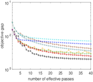
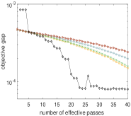
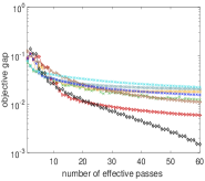
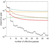
SAG-ADMM Zhong & Kwok (2014) and SVRG-ADMM Zheng & Kwok (2016) accelerate SADMM to ergodic O(1/K)𝑂1𝐾O(1/K). In Theorem 999 of Li & Lin (2016), the authors generate a class of functions showing that the original ADMM has a tight non-ergodic O(1/K)𝑂1𝐾O(1/\sqrt{K}) convergence rate. When n=1𝑛1n=1, SAG-ADMM and SVRG-ADMM are the same as batch ADMM, so their convergence rates are no better than O(1/K)𝑂1𝐾O(1/\sqrt{K}). This shows that our algorithm has a faster convergence rate than VR based SADMM methods in non-ergodic sense. One may deem that judging convergence in ergodic or non-ergodic is unimportant in practice. However, in experiments, our algorithm is much faster than VR based SADMM methods. Actually, though VR based SADMM methods have provably faster rates than STOC-ADMM, the improvement in practice is evident only iterates are close to the convergence point, rather than at the early stage. Both Zhong & Kwok (2014) and Zheng & Kwok (2016) show that SAG-ADMM and SVRG-ADMM are sensitive to the initial points. We also find that if the step sizes are set based on the their theoretical guidances, sometimes they are even slower than STOC-ADMM (see Fig. 1) as the early stage lasts longer when the step size is small. Our algorithm is faster than the two algorithms whenever the step sizes are set based on the theoretical guidances or are tuned to achieve the fastest speed (see Fig. 2). This demonstrates that Nesterov’s extrapolation has truly accelerated the speed and the integration of extrapolation and VR techniques is harmonious and complementary.
Refer to caption
(a) a9a-training
Refer to caption
(b) covertype-training
Refer to caption
(c) mnist-training
Refer to caption
(d) dna-training
Refer to caption
(e) a9a-testing
Refer to caption
(f) covertype-testing
Refer to caption
(g) mnist-testing
Refer to caption
(h) dna-testing
Refer to caption
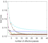
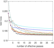
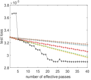
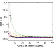
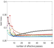
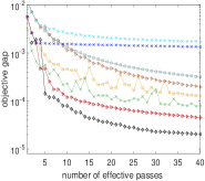
Figure 1: Experimental results of solving the original Lasso problem (Eq. (23)) (Top: objective gap; Bottom: testing loss). The step sizes are set based on the theoretical guidances. The computation time has included the cost of calculating full gradients for SVRG based methods. SVRG-ADMM and SAG-ADMM are initialized by running STOC-ADMM for 3nb3𝑛𝑏\frac{3n}{b} iterations. “-ERG” represents the ergodic results for the corresponding algorithms.
Refer to caption
(a) a9a-training
Refer to caption
(b) covertype-training
Refer to caption
(c) mnist-training
Refer to caption
(d) dna-training
Refer to caption
(e) a9a-testing
Refer to caption
(f) covertype-testing
Refer to caption
(g) mnist-testing
Refer to caption
(h) dna-testing
Refer to caption
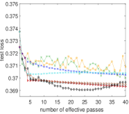
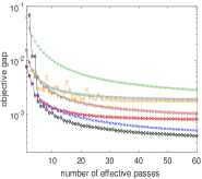
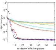
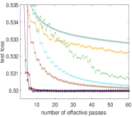
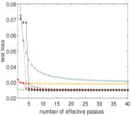
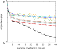
Figure 2: Experimental results of solving the Graph-Guided Fused Lasso problem (Eq. (24)) (Top: objective gap; Bottom: testing loss). The step size is tuned to be the best for each algorithm. The computation time has included the cost of calculating full gradients for SVRG based methods. SVRG-ADMM and SAG-ADMM are initialized by running STOC-ADMM for 3nb3𝑛𝑏\frac{3n}{b} iterations. “-ERG” represents the ergodic results for the corresponding algorithms.

5.3 The Growth of Penalty Factor βθ1s𝛽superscriptsubscript𝜃1𝑠\frac{\beta}{\theta_{1}^{s}}

One can find that the penalty factor βθ1s𝛽superscriptsubscript𝜃1𝑠\frac{\beta}{\theta_{1}^{s}} increases linearly with the iteration. This might make our algorithm impractical because after dozens of epoches, the large value of penalty factor might slow down the decrement of function value. However, in experiments, we have not found any bad influence. There may be two reasons 1. In our algorithm, θ1,ssubscript𝜃1𝑠\theta_{1,s} decreases after each epoch (m𝑚m iterations), which is much slower than LADM-NE Li & Lin (2016). For most stochastic problems, algorithms converge in less than 100100100 epoches, thus θ1,ssubscript𝜃1𝑠\theta_{1,s} is only 200200200 times of θ1,0subscript𝜃10\theta_{1,0}. The growth of penalty factor works as a continuation technique Zuo & Lin (2011), which may help to decrease the function value. 2. From Theorem 1, our algorithm converges in O(1/S)𝑂1𝑆O(1/S) whenever θ1,ssubscript𝜃1𝑠\theta_{1,s} is large. So from the theoretical viewpoint, a large θ1,ssubscript𝜃1𝑠\theta_{1,s} cannot slow down our algorithm. We find that OPT-ADMM AzadiSra & Sra (2014) also needs to decrease the step size with the iteration. However, its step size decreasing rate is O(k32)𝑂superscript𝑘32O(k^{\frac{3}{2}}) and is faster than ours.

6 Experiments

We conduct experiments to show the effectiveness of our method222We will put our code online once our paper is accepted.. We compare our method with the following the-state-of-the-art SADMM algorithms: (1) STOC-ADMM Ouyang et al. (2013), (2) SVRG-ADMM Zheng & Kwok (2016), (3) OPT-SADMM AzadiSra & Sra (2014), (4) SAG-ADMM Zhong & Kwok (2014). We ignore the comparison with SDCA-ADMM Suzuki (2014) since there is no analysis for it on general convex problems and it is also not faster than SVRG-ADMM Zheng & Kwok (2016). Experiments are performed on Intel(R) CPU i7-4770 @ 3.40GHz machine with 161616 GB memory.

6.1 Lasso Problems

We perform experiments to solve two typical Lasso problems. The first is the original Lasso problem:

min𝐱μ𝐱1+1ni=1nhi𝐱Tai2,subscript𝐱𝜇subscriptnorm𝐱11𝑛superscriptsubscript𝑖1𝑛superscriptnormsubscript𝑖superscript𝐱𝑇subscript𝑎𝑖2\displaystyle\min_{\mathbf{x}}\mu\|\mathbf{x}\|_{1}+\frac{1}{n}\sum_{i=1}^{n}\|h_{i}-\mathbf{x}^{T}a_{i}\|^{2}, (23)

where 𝐡isubscript𝐡𝑖\mathbf{h}_{i} and 𝐚isubscript𝐚𝑖\mathbf{a}_{i} are the tag and the data vector, respectively. The second is Graph-Guided Fused Lasso model:

min𝐱μ𝐀𝐱1+1ni=1nli(𝐱),subscript𝐱𝜇subscriptnorm𝐀𝐱11𝑛superscriptsubscript𝑖1𝑛subscript𝑙𝑖𝐱\displaystyle\min_{\mathbf{x}}\mu\|\mathbf{A}\mathbf{x}\|_{1}+\frac{1}{n}\sum_{i=1}^{n}l_{i}(\mathbf{x}), (24)

where li(𝐱)subscript𝑙𝑖𝐱l_{i}(\mathbf{x}) is the logistic loss on sample i𝑖i, and 𝐀=[𝐆;𝐈]𝐀𝐆𝐈\mathbf{A}=[\mathbf{G};\mathbf{I}] is a matrix encoding the feature sparsity pattern. 𝐆𝐆\mathbf{G} is the sparsity pattern of the graph obtained by sparse inverse covariance estimation Friedman et al. (2008). The experiments are performed on four benchmark data sets: a9a, covertype, mnist and dna333a9a, covertype and dna are from: http://www.csie.ntu.edu.tw/~cjlin/libsvmtools/datasets/, and mnist is from: http://yann.lecun.com/exdb/mnist/.. The details of the dataset and the mini-batch size that we use in all SADMM are shown in Table 2. And like Zhong & Kwok (2014) and  Zheng & Kwok (2016), we fix μ𝜇\mu to be 105superscript10510^{-5} and report the performance based on (𝐱t,𝐀𝐱t)subscript𝐱𝑡subscript𝐀𝐱𝑡(\mathbf{x}_{t},\mathbf{A}\mathbf{x}_{t}) to satisfy the constraints of ADMM. Results are averaged over five repetitions. And we set m=2nb𝑚2𝑛𝑏m=\frac{2n}{b} for all the algorithms. To solve the problems by ADMM methods, we introduce an variable 𝐲=𝐱𝐲𝐱\mathbf{y}=\mathbf{x} or 𝐲=𝐀𝐱𝐲𝐀𝐱\mathbf{y}=\mathbf{A}\mathbf{x}. The update for 𝐱𝐱\mathbf{x} can be written as: 𝐱k+1=𝐱kγ(~f2(𝐱2)+β𝐀T(𝐀𝐱𝐲)+𝐀T𝝀)superscript𝐱𝑘1superscript𝐱𝑘𝛾~subscript𝑓2subscript𝐱2𝛽superscript𝐀𝑇𝐀𝐱𝐲superscript𝐀𝑇𝝀\mathbf{x}^{k+1}=\mathbf{x}^{k}-\gamma(\tilde{\nabla}f_{2}(\mathbf{x}_{2})+\beta\mathbf{A}^{T}(\mathbf{A}\mathbf{x}-\mathbf{y})+\mathbf{A}^{T}\bm{\lambda}), where γ𝛾\gamma is the step size, which depends on the penalty factor β𝛽\beta and the Lipschitz constant L2subscript𝐿2L_{2}. For the original Lasso (Eq (23)), L2subscript𝐿2L_{2} has a closed-form solution, namely, we set L2=maxiai2=1subscript𝐿2subscript𝑖superscriptnormsubscript𝑎𝑖21L_{2}=\max_{i}\|a_{i}\|^{2}=1444We normalize the Frobenius norm of each feature to 1.. So in this task, the step sizes are set through theoretical guidances for each algorithm. For Graph-Guided Fused Lasso (Eq (24)), we regard L2subscript𝐿2L_{2} as a tunable parameter and tune L2subscript𝐿2L_{2} to obtain the best step size for each algorithm, which is similar to Zheng & Kwok (2016) and Zhong & Kwok (2014). Except ACC-SADMM, we use the continuation technique Zuo & Lin (2011) to accelerate algorithms. We set βs=min(10,ρsβ0)subscript𝛽𝑠10superscript𝜌𝑠subscript𝛽0\beta_{s}=\min(10,\rho^{s}\beta_{0}). Since SAG-ADMM and SVRG-ADMM are sensitive to initial points, like Zheng & Kwok (2016), they are initialized by running STOC-ADMM for 3nb3𝑛𝑏\frac{3n}{b} iterations. SAG-ADMM is performed on the first three datasets due to its large memory requirement. More details about parameter setting can be found in Supplementary Materials.

The experimental results of original Lasso and Graph-Guided Fused Lasso are shown in Fig. 1 and Fig. 2, respectively. From the results, we can find that SVRG-ADMM performs much better than STOC-ADMM when the step size is large while the improvement is not large when the step size is small as it has the cost of calculating the full gradient. SAG-ADMM encounters a similar situation as 𝐱𝐱\mathbf{x} is not updated on the latest information. OPT-ADMM performs well on the small step size. However, when the step size is large, the noise of the gradients limits the effectiveness of the extrapolation. Our algorithm is faster than other SADMM on both problems. More experimental results where we set a larger fixed step size and the memory costs of all algorithms are shown in Supplementary Materials.
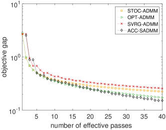
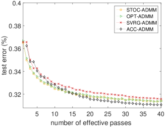
Refer to caption
(a) objective gap vs. iteration
Refer to caption
(b) test error vs. iteration
Figure 3: The experimental result of Multitask Learning.
Table 2: Details of datasets. (Dim., Cla, and mini., are short for dimensionality, class, and mini-batch, respectively. Las. is short for the Lasso problem. Mul. is short for Multitask Learning.).
Pro. Dataset # training # testing Dim. ×\times Cla. # mini.
Las. a9a 72,8767287672,876 72,8757287572,875 74×274274\times 2 100100100
covertype 290,506290506290,506 290,506290506290,506 54×254254\times 2
mnist 60,0006000060,000 10,0001000010,000 784×1078410784\times 10
dna 2,400,00024000002,400,000 600,000600000600,000 800×28002800\times 2 500500500
Mul. ImageNet 1,281,16712811671,281,167 50,0005000050,000 4,096×1,000409610004,096\times 1,000 2,00020002,000

6.2 Multitask Learning

We perform experiments on multitask learning Argyriou et al. (2007). A similar experiment is also conducted by Zheng & Kwok (2016). The experiment is performed on a 1000-class ImageNet dataset Russakovsky et al. (2015) (see Table 2). The features are generated from the last fully connected layer of the convolutional VGG-16 net Simonyan & Zisserman (2014). More detailed descriptions on the problem are shown in Supplementary Materials.

Fig. 3 shows the objective gap and test error against iteration. Our method is also faster than other SADMM.

7 Conclusion

We propose ACC-SADMM for the general convex finite-sum problems. ACC-SADMM integrates Nesterov’s extrapolation and VR techniques and achieves a non-ergodic O(1/K)𝑂1𝐾O(1/K) convergence rate. We do experiments to demonstrate that our algorithm is faster than other SADMM.

References

  • Allen-Zhu (2017) Allen-Zhu, Zeyuan. Katyusha: The first truly accelerated stochastic gradient method. In Annual Symposium on the Theory of Computing, 2017.
  • Argyriou et al. (2007) Argyriou, Andreas, Evgeniou, Theodoros, and Pontil, Massimiliano. Multi-task feature learning. Proc. Conf. Advances in Neural Information Processing Systems, 2007.
  • AzadiSra & Sra (2014) AzadiSra, Samaneh and Sra, Suvrit. Towards an optimal stochastic alternating direction method of multipliers. In Proc. Int’l. Conf. on Machine Learning, 2014.
  • Beck & Teboulle (2009) Beck, Amir and Teboulle, Marc. A fast iterative shrinkage-thresholding algorithm for linear inverse problems. SIAM Journal on Imaging Sciences, 2(1):183–202, 2009.
  • Bottou (2004) Bottou, Léon. Stochastic learning. In Advanced lectures on machine learning, pp.  146–168. 2004.
  • Boyd et al. (2011) Boyd, Stephen, Parikh, Neal, Chu, Eric, Peleato, Borja, and Eckstein, Jonathan. Distributed optimization and statistical learning via the alternating direction method of multipliers. Foundations and Trends® in Machine Learning, 3(1):1–122, 2011.
  • Chen et al. (2015) Chen, Caihua, Chan, Raymond H, Ma, Shiqian, and Yang, Junfeng. Inertial proximal ADMM for linearly constrained separable convex optimization. SIAM Journal on Imaging Sciences, 8(4):2239–2267, 2015.
  • Davis & Yin (2016) Davis, Damek and Yin, Wotao. Convergence rate analysis of several splitting schemes. In Splitting Methods in Communication, Imaging, Science, and Engineering, pp.  115–163. 2016.
  • Defazio et al. (2014) Defazio, Aaron, Bach, Francis, and Lacoste-Julien, Simon. SAGA: A fast incremental gradient method with support for non-strongly convex composite objectives. In Proc. Conf. Advances in Neural Information Processing Systems, 2014.
  • Friedman et al. (2008) Friedman, Jerome, Hastie, Trevor, and Tibshirani, Robert. Sparse inverse covariance estimation with the graphical lasso. Biostatistics, 9(3):432–441, 2008.
  • Frostig et al. (2015) Frostig, Roy, Ge, Rong, Kakade, Sham, and Sidford, Aaron. Un-regularizing: approximate proximal point and faster stochastic algorithms for empirical risk minimization. In Proc. Int’l. Conf. on Machine Learning, 2015.
  • He & Yuan (2012) He, Bingsheng and Yuan, Xiaoming. On the O(1/n)𝑂1𝑛{O}(1/n) convergence rate of the Douglas–Rachford alternating direction method. SIAM Journal on Numerical Analysis, 50(2):700–709, 2012.
  • Hien et al. (2016) Hien, Le Thi Khanh, Lu, Canyi, Xu, Huan, and Feng, Jiashi. Accelerated stochastic mirror descent algorithms for composite non-strongly convex optimization. arXiv preprint arXiv:1605.06892, 2016.
  • Johnson & Zhang (2013) Johnson, Rie and Zhang, Tong. Accelerating stochastic gradient descent using predictive variance reduction. In Proc. Conf. Advances in Neural Information Processing Systems, 2013.
  • Kim et al. (2009) Kim, Seyoung, Sohn, Kyung-Ah, and Xing, Eric P. A multivariate regression approach to association analysis of a quantitative trait network. Bioinformatics, 25(12):i204–i212, 2009.
  • Li & Lin (2016) Li, Huan and Lin, Zhouchen. Optimal nonergodic O(1/k)𝑂1𝑘{O}(1/k) convergence rate: When linearized ADM meets nesterov’s extrapolation. arXiv preprint arXiv:1608.06366, 2016.
  • Lin et al. (2015a) Lin, Hongzhou, Mairal, Julien, and Harchaoui, Zaid. A universal catalyst for first-order optimization. In Proc. Conf. Advances in Neural Information Processing Systems, 2015a.
  • Lin et al. (2011) Lin, Zhouchen, Liu, Risheng, and Su, Zhixun. Linearized alternating direction method with adaptive penalty for low-rank representation. In Proc. Conf. Advances in Neural Information Processing Systems, 2011.
  • Lin et al. (2015b) Lin, Zhouchen, Liu, Risheng, and Li, Huan. Linearized alternating direction method with parallel splitting and adaptive penalty for separable convex programs in machine learning. Machine Learning, 99(2):287–325, 2015b.
  • Lu et al. (2016) Lu, Canyi, Li, Huan, Lin, Zhouchen, and Yan, Shuicheng. Fast proximal linearized alternating direction method of multiplier with parallel splitting. In Proc. AAAI Conf. on Artificial Intelligence, 2016.
  • Nesterov (1983) Nesterov, Yurii. A method for unconstrained convex minimization problem with the rate of convergence O(1/k2)𝑂1superscript𝑘2{O}(1/k^{2}). In Doklady an SSSR, volume 269, pp.  543–547, 1983.
  • Nesterov (1988) Nesterov, Yurii. On an approach to the construction of optimal methods of minimization of smooth convex functions. Ekonomika i Mateaticheskie Metody, 24(3):509–517, 1988.
  • Nesterov (2013) Nesterov, Yurii. Introductory lectures on convex optimization: A basic course, volume 87. 2013.
  • Nitanda (2014) Nitanda, Atsushi. Stochastic proximal gradient descent with acceleration techniques. In Proc. Conf. Advances in Neural Information Processing Systems, 2014.
  • Ouyang et al. (2013) Ouyang, Hua, He, Niao, Tran, Long, and Gray, Alexander G. Stochastic alternating direction method of multipliers. Proc. Int’l. Conf. on Machine Learning, 2013.
  • Ouyang et al. (2015) Ouyang, Yuyuan, Chen, Yunmei, Lan, Guanghui, and Pasiliao Jr, Eduardo. An accelerated linearized alternating direction method of multipliers. SIAM Journal on Imaging Sciences, 8(1):644–681, 2015.
  • Russakovsky et al. (2015) Russakovsky, Olga, Deng, Jia, Su, Hao, Krause, Jonathan, Satheesh, Sanjeev, Ma, Sean, Huang, Zhiheng, Karpathy, Andrej, Khosla, Aditya, Bernstein, Michael, et al. Imagenet large scale visual recognition challenge. Int’l. Journal of Computer Vision, 115(3):211–252, 2015.
  • Schmidt et al. (2013) Schmidt, Mark, Le Roux, Nicolas, and Bach, Francis. Minimizing finite sums with the stochastic average gradient. Mathematical Programming, pp.  1–30, 2013.
  • Shen et al. (2015) Shen, Li, Sun, Gang, Lin, Zhouchen, Huang, Qingming, and Wu, Enhua. Adaptive sharing for image classification. In Proc. Int’l. Joint Conf. on Artificial Intelligence, 2015.
  • Simonyan & Zisserman (2014) Simonyan, Karen and Zisserman, Andrew. Very deep convolutional networks for large-scale image recognition. arXiv preprint arXiv:1409.1556, 2014.
  • Suzuki (2013) Suzuki, Taiji. Dual averaging and proximal gradient descent for online alternating direction multiplier method. In Proc. Int’l. Conf. on Machine Learning, 2013.
  • Suzuki (2014) Suzuki, Taiji. Stochastic dual coordinate ascent with alternating direction method of multipliers. In Proc. Int’l. Conf. on Machine Learning, 2014.
  • Tseng (2008) Tseng, Paul. On accelerated proximal gradient methods for convex-concave optimization. In Technical report, 2008.
  • Wang et al. (2016) Wang, Kaiye, He, Ran, Wang, Liang, Wang, Wei, and Tan, Tieniu. Joint feature selection and subspace learning for cross-modal retrieval. IEEE Trans. on Pattern Analysis and Machine Intelligence, 38(10):1–1, 2016.
  • Zhang et al. (2011) Zhang, Xiaoqun, Burger, Martin, and Osher, Stanley. A unified primal-dual algorithm framework based on bregman iteration. Journal of Scientific Computing, 46:20–46, 2011.
  • Zheng & Kwok (2016) Zheng, Shuai and Kwok, James T. Fast-and-light stochastic admm. In Proc. Int’l. Joint Conf. on Artificial Intelligence, 2016.
  • Zhong & Kwok (2014) Zhong, Wenliang and Kwok, James Tin-Yau. Fast stochastic alternating direction method of multipliers. In Proc. Int’l. Conf. on Machine Learning, 2014.
  • Zuo & Lin (2011) Zuo, Wangmeng and Lin, Zhouchen. A generalized accelerated proximal gradient approach for total variation-based image restoration. IEEE Trans. on Image Processing, 20(10):2748, 2011.