A Nuclear-norm Model for Multi-Frame Super-Resolution Reconstruction from Video Clips

Abstract

We propose a variational approach to obtain super-resolution images from multiple low-resolution frames extracted from video clips. First the displacement between the low-resolution frames and the reference frame are computed by an optical flow algorithm. Then a low-rank model is used to construct the reference frame in high-resolution by incorporating the information of the low-resolution frames. The model has two terms: a 2-norm data fidelity term and a nuclear-norm regularization term. Alternating direction method of multipliers is used to solve the model. Comparison of our methods with other models on synthetic and real video clips show that our resulting images are more accurate with less artifacts. It also provides much finer and discernable details.

I Introduction

Super-resolution (SR) image reconstruction from multiple low-resolution (LR) frames have many applications, such as in remote sensing, surveillance, and medical imaging. After the pioneering work of Tsai and Huang [1], SR image reconstruction has become more and more popular in image processing community, see for examples [2, 3, 4, 5, 6, 7, 8, 9]. SR image reconstruction problems can be classified into two categories: single-frame super-resolution problems (SFSR) and multi-frame super-resolution problems (MFSR). In this paper, we mainly focus on the multi-frame case, especially the MFSR problems from low-resolution video sequences. Below, we first review some existing work related to MFSR problems.

Bose and Boo [2] considered the case where the multiple LR image frames were shifted with affine transformations. They modeled the original high-resolution (HR) image as a stationary Markov-Gaussian random field. Then they made use of the maximum a posteriori scheme to solve their model. However the affine transformation assumption may not be satisfied in practice, for example when there are complex motions or illumination changes. Another approach for SR image reconstruction is the one known as patch-based or learning-based. Bishop et al. [10] used a set of learned image patches which capture the information between the middle and high spatial frequency bands. They assumed a priori distribution over such patches and made use of the previous enhanced frame to provide part of the training set. The disadvantage of this patch-based method is that it is usually time consuming and sensitive to the off-line training set. Liu and Sun [11] applied Bayessian approach to estimate simultaneously the underlying motion, the blurring kernel, the noise level and the HR image. Within each iteration, they estimated the motion, the blurring kernel and the HR image alternatively by maximizing a posteriori respectively. Based on this work, Ma et al. [12] tackled motion blur in their paper. An expectation maximization (EM) framework is applied to the Bayessian approach to guide the estimation of motion blur. These methods used optical flow to model the motion between different frames. However they are sensitive to the accuracy of flow estimation. The results may fail when the noise is heavy.

In [13], Chan et al. applied wavelet analysis to HR image reconstruction. They decomposed the image from previous iteration into wavelet frequency domain and applied wavelet thresholding to denoise the resulting images. Based on this model, Chan et al. [14] later developed an iterative MFSR approach by using tight-frame wavelet filters. However because of the number of framelets involved in analyzing the LR images, the algorithm can be extremely time consuming.

Optimization models are one of the most important image processing models. Following the classical ROF model [15], Farsiu et al. [16] proposed a total variation-$l_{1}$ model where they used the $l_{1}$ norm for the super-resolution data fidelity term. However it is known that TV regularization enforces a piecewise solution. Therefore their method will produce some artifacts. Li, Dai and Shen [17] used $l_{1}$ norm of the geometric tight-framelet coefficients as the regularizer and adaptively mimicking $l_{1}$ and $l_{2}$ norms as the data fidelity term. They also assumed affine motions between different frames. The results are therefore not good when complex motions or illumination changes are involved.

Chen and Qi [18] recently proposed a single-frame HR image reconstruction method via low rank regularization. Jin et al. [19] designed a patch based low rank matrix completion algorithm from the sparse representation of LR images. The main idea of these two papers is based on the assumption that each LR image is downsampled from a blurred and shifted HR image. However these work assumed that the original HR image, when considered as a matrix, has a low rank property, which is not convincing in general.

In this paper, we show that the low rank property can in fact be constructed under MFSR framework. The idea is to consider each LR image as a downsampled instance of a different blurred and shifted HR image. Then when all these different HR images are properly aligned, they should give a low rank matrix; and therefore we can use a low rank prior to obtain a better solution. Many existing work assumes the shift between two consecutive LR frames are small, see, e.g., [20, 16, 21, 22, 23]. In this paper, we allow illumination changes and more complex motions other than affine transformation. They are handled by an optical flow model proposed in [24]. Once the motions are determined, we reconstruct the high-resolution image by minimizing a functional which consists of two terms: the 2-norm data fidelity term to suppress Gaussian noise and a nuclear-norm regularizer to enforce the low-rank prior. Tests on seven synthetic and real video clips show that our resulting images is more accurate with less artifacts. It can also provide much finer and discernable details.

The rest of the paper is organized as follows. Section II gives a brief review of a classical model on modeling LR images from HR images. Our model will be based on this model. Section III provides the details of our low-rank model, including image registration by optical flow and the solution of our optimization problem by alternating direction method. Section IV gives experimental results on the test videos. Conclusions are given in Section V.

To simplify our discussion, we now give the notation that we will be using for the rest of the paper. For any integer $m\in\mathbb{Z}$, $I_{m}$ is the $m\times m$ identity matrix. For any integer $l\in\mathbb{Z}$ and positive integer $n\in\mathbb{Z}^{+}$, there exists a unique $0\leq\widetilde{l}<n$ such that $\widetilde{l}\equiv l\mod n$. Let $N_{n}(l)$ denote the $n\times n$ matrix

$${N}_{n}(l)=\left[\begin{array}[]{cc}0&I_{n-\widetilde{l}}\\ I_{\widetilde{l}}&0\end{array}\right].$$ (1)

For a vector $\mathbf{f}\in\mathbb{R}^{n}$, $N_{n}(l)\mathbf{f}$ is the vector with entries of $\mathbf{f}$ cyclic-shifted by $l$.

Define the downsampling matrix $D_{i}$ and the upsampling matrix $D^{T}_{i}$ as

$$D_{i}(n)=I_{n}\otimes\mathbf{e}_{i}^{T}\text{ and }D^{T}_{i}(n)=I_{n}\otimes\mathbf{e}_{i},~{}i=0,1,$$ (2)

where $\mathbf{e}_{0}=[1,0]^{T},\mathbf{e}_{1}=[0,1]^{T}$ and $\otimes$ is the Kronecker product. For $0\leq\epsilon\leq 1$, define $T_{n}(\epsilon)$ to be the $n\times n$ Toeplitz matrix

$$T_{n}(\epsilon)=\left[\begin{array}[]{ccccc}1-\epsilon&\epsilon&\cdots&0\\ 0&1-\epsilon&\ddots&\vdots\\ \vdots&\ddots&\ddots&\epsilon\\ \epsilon&\cdots&0&1-\epsilon\end{array}\right].$$ (3)

This Toeplitz matrix performs the effect of linear interpolation shifted by $\epsilon$.

II Low resolution model with shifts

Consider a LR sensor array recording a video of an object. Then it gives multiple LR images of the object. Unless the object or the sensor array is completely motionless during the recording, the LR images will contain multiple information of the object at different shifted locations (either because of the motion of the object or of the sensor array itself). Our problem is to improve the resolution of one of the LR images (called the reference image) by incorporating information from the other LR images.

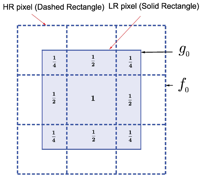
Let the sensor array consist of $m\times n$ sensing elements, where the width and the height of each sensing element is $L_{x}$ and $L_{y}$ respectively. Then, the sensor array will produce an $m\times n$ discrete image with $mn$ pixels where each of these LR pixels is of size $L_{x}\times L_{y}$. Let $r$ be the upsampling factor, i.e. we would like to construct an image of resolution $rm\times rn$ of the same scene. Then the size of the HR pixels will be $L_{x}/r\times L_{y}/r$. Fig 1(a) shows an example. The big rectangles with solid edges are the LR pixels and the small rectangles with dashed edges are the HR pixels.

(a) Displacements between LR images

(b) The averaging process

Figure 1: LR Images with displacements

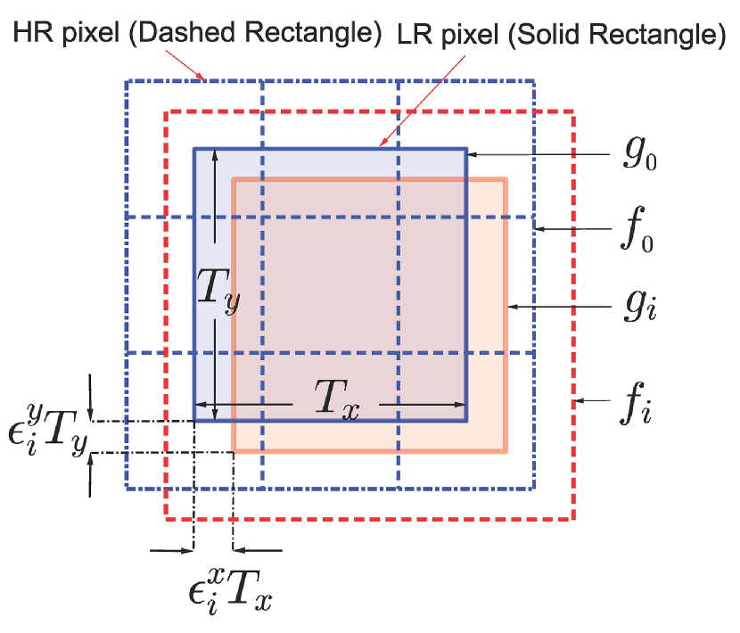
Let $\{g_{i}\in\mathbb{R}^{m\times n},1\leq i\leq p\}$ be the sequence of LR images produced by the sensor array at different time points, where $p$ is the number of frames. For simplicity we let $g_{0}$ be the reference LR image which can be chosen to be any one of the LR images $g_{i}$. The displacement of $g_{i}$ from the reference image $g_{0}$ is denoted by $(\epsilon^{x}_{i}L_{x},\epsilon^{y}_{i}L_{y})$, see the solid rectangle in Fig. 1(a) labeled as $g_{i}$. For ease of notation, we will represent the 2D images $g_{i}$, $0\leq i\leq p$, by vectors $\mathbf{g}_{i}\in\mathbb{R}^{mn}$ obtained by stacking the columns of $g_{i}$. We use $\mathbf{f}\in\mathbb{R}^{r^{2}mn}$ to denote the HR reconstruction of $g_{0}$ that we are seeking.

We model the relationship between $\mathbf{f}$ and $\mathbf{g}_{0}$ by averaging, see [2, 6]. Fig. 1(b) illustrates that the intensity value of the LR pixel is the weighted average of the intensity values of the HR pixels overlapping with it. The weight is precisely the area of overlapping. Thus the process from $\mathbf{f}$ to each of the LR images $g_{i}$ can be modeled by [6]:

$$\mathbf{g}_{i}=DKA_{i}\mathbf{f}+\mathbf{n}_{i},~{}i=1,2,\cdots,p,$$ (4)

where $D=D_{0}(n)\otimes D_{0}(m)\in\mathbb{R}^{mn\times r^{2}mn}$ is the downsampling matrix defined by (2); $K\in\mathbb{R}^{r^{2}mn\times r^{2}mn}$ is the average operator mentioned above; $A_{i}\in\mathbb{R}^{r^{2}mn\times r^{2}mn}$ is the warping matrix which measures the displacement between $g_{i}$ and $g_{0}$; and $\mathbf{n}_{i}$ is the additive unknown noise. In this paper, we assume for simplicity the noise are Gaussian. Other noise models can be handled by choosing suitable data fidelity terms.

The warping matrix $A_{i}$, $1\leq i\leq p$, is to align the LR pixels in $\mathbf{g}_{i}$ at exactly the middle of the corresponding HR pixels in $\mathbf{f}$, exactly like the $\mathbf{g}_{0}$ is w.r.t $\mathbf{f}_{0}$ in Fig. 1(b). Once this alignment is done, the average operator $K$, which is just a blurring operator, can be written out easily. In fact, the 2D kernel (i.e. the point spread function) of $K$ is given by $vv^{T}$, where $v=[1/2,1,\ldots,1,1/2]^{T}$ with $(r-1)$ ones in the middle, see [2]. The $A_{i}$ are more difficult to obtain. In the most ideal case where the motions are only translation of less than one HR pixel length and width, $A_{i}$ can be modeled by $A_{i}=T_{n}(\epsilon_{i}^{x})\otimes T_{m}(\epsilon_{i}^{y})$, where $T_{n}(\epsilon_{i}^{x}),T_{m}(\epsilon_{i}^{y})$ are Toeplitz matrices given by (3) with $(\epsilon^{x}_{i}L_{x},\epsilon^{y}_{i}L_{y})$ being the horizontal and vertical displacements of $g_{i}$, see Fig. 1(a) and [6]. In reality, the changes between different LR frames are much more complicated. It can involve illumination changes and other complex non-planar motions. We will discuss the formation of $A_{i}$ in more details in Subsections III-A and III-C.

III Nuclear model

Given (4), a way to obtain $\mathbf{f}$ is to minimize the noise $\mathbf{n}_{i}$ by least-squares. However because $D$ is singular, the problem is ill-posed. Regularization is necessary to make use of some priori information to choose the correct solution. A typical regularizer for solving this problem is Total Variation (TV) [15]. The TV model is well known for edge preserving and can give a reasonable solution for MFSR problems. However it assumes that the HR image is piecewise constant. This will produce some artifacts.

Instead we will develop a low-rank model for the problem. The main motivation is as follows. We consider each LR image $\mathbf{g}_{i}$ as a downsampled version of an HR image $\mathbf{f}_{i}$. If all these HR images $\mathbf{f}_{i}$ are properly aligned with the HR image $\mathbf{f}$, then they all should be the same exactly (as they are representing the same scene $\mathbf{f}$). In particular, if $A_{i}$ is the alignment matrix that aligns $\mathbf{f}_{i}$ with $\mathbf{f}$, then the matrix $[A_{1}\mathbf{f}_{1},A_{2}\mathbf{f}_{2},\ldots,A_{p}\mathbf{f}_{p}]$ should be a low rank matrix (ideally a rank 1 matrix). Thus the rank of the matrix can be used as a prior.

In Subsection III-A, we introduce our low-rank model in the case where the LR images are perturbed only by translations. Then in Subsection III-B, we explain how to solve the model by the alternating direction method. In Subsection III-C, we discuss how to modify the model when there are more complex motions or changes between the LR frames.

III-A Decomposition of the warping matrices

In order to introduce our model without too cumbersome notations, we assume first here that the displacements of the LR images from the reference frame are translations only. Let $s_{i}^{x}L_{x}$ and $s_{i}^{y}L_{y}$ be the horizontal and vertical displacements of $g_{i}$ from $g_{0}$. (How to obtain $s_{i}^{x}$ and $s_{i}^{y}$ will be discussed in Subsection III-C.) Since the width and height of one HR pixel are $L_{x}/r$ and $L_{y}/r$ respectively, the displacements are equivalent to $rs_{i}^{x}$ HR pixel length and $rs_{i}^{y}$ HR pixel width. We decompose $rs_{i}^{x}$ and $rs_{i}^{y}$ into the integral parts and fractional parts:

$$rs_{i}^{x}=l_{i}^{x}+\epsilon_{i}^{x},~{}rs_{i}^{y}=l_{i}^{y}+\epsilon_{i}^{y},$$ (5)

where $l_{i}^{x},l_{i}^{y}$ are integers and $0\leq\epsilon_{i}^{x},\epsilon_{i}^{x}<1$. Then the warping matrix can be decomposed as:

$$A_{i}=C_{i}B_{i},$$ (6)

where $B_{i}=N_{n}(l_{i}^{x})\otimes N_{m}(l_{i}^{y})$ is given by (1) and $C_{i}=T_{n}(\epsilon_{i}^{x})\otimes T_{m}(\epsilon_{i}^{y})$ is given by (3) [13]. Thus by letting $\mathbf{f}_{i}=B_{i}\mathbf{f}$, $1\leq i\leq p$, (4) can be rewritten as

$$\mathbf{g}_{i}=DKC_{i}\mathbf{f}_{i}+\mathbf{n}_{i},~{}i=1,2,\cdots,p.$$ (7)

As mentioned in the motivation above, all these $\mathbf{f}_{i}$, which are equal to $B_{i}\mathbf{f}$, are integral shift from $\mathbf{f}$. Hence if they are aligned correctly by an alignment matrix $W_{i}$, then the overlapping entries should be the same. Fig. 2 is the 1D illustration of this idea. The $W_{i}^{x}$ is the matrix that aligns $\mathbf{f}_{i}$ with $\mathbf{f}$ (in the $x$-direction) and the dark squares are the overlapping pixels and they should all be the same as the corresponding pixels in $\mathbf{f}$.

Figure 2: $1$-D signals with integer displacements

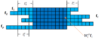
Mathematically, $W_{i}$ is constructed as follows. Given the decomposition of $rs_{i}^{x}$ and $rs_{i}^{y}$ in (5), let $l_{+}^{x}=\max_{i}\{0,l_{i}^{x}\}$, $l_{+}^{y}=\max_{i}\{0,l_{i}^{y}\}$, and $l_{-}^{x}=\max_{i}\{0,-l_{i}^{x}\}$, $l_{-}^{y}=\max_{i}\{0,-l_{i}^{y}\}$. Then

$$W_{i}=W_{i}^{x}\otimes W_{i}^{y}.$$ (8)

where

$$W_{i}^{x}=\left[\begin{array}[]{ccc}0_{l_{+}^{x}-l_{i}^{x}}&&\\ &I_{rn-l_{+}^{x}-l_{-}^{x}}&\\ &&0_{l_{-}^{x}+l_{i}^{x}}\end{array}\right],$$

$$W_{i}^{y}=\left[\begin{array}[]{ccc}0_{l_{+}^{y}-l_{i}^{y}}&&\\ &I_{rm-l_{+}^{y}-l_{-}^{y}}&\\ &&0_{l_{-}^{y}+l_{i}^{y}}\end{array}\right].$$

Note that $W_{i}$ nullifies the entries outside the overlapping part (i.e. outside the dark squares in Fig. 2).

Ideally, the matrix $[W_{1}\mathbf{f}_{1},W_{2}\mathbf{f}_{2},\cdots,W_{p}\mathbf{f}_{p}]$ should be a rank-one matrix as every column should be a replicate of $\mathbf{f}$ in the overlapping region. In practice, it can be of low rank due to various reasons such as errors in measurements and noise in the given video. Since nuclear norm is the convexification of low rank prior, see [25], this leads to our convex model

$$\min_{\mathbf{f}_{1},\cdots,\mathbf{f}_{p}}\lambda\|W_{1}\mathbf{f}_{1},W_{2}\mathbf{f}_{2},\cdots,W_{p}\mathbf{f}_{p}\|_{*}+\frac{1}{2}\sum_{i=1}^{p}\|\mathbf{g}_{i}-DKC_{i}\mathbf{f}_{i}\|_{2}^{2},$$ (9)

where $\|\cdot\|_{*}$ is the matrix nuclear norm and $\lambda$ is the regularization parameter. We call our model (9) the nuclear model. We remark that here we use the 2-norm data fidelity term because we assume the noise are Gaussian. It can be changed to another norm according to the noise type.

III-B Algorithm for solving the nuclear model

We use alternating direction method of multipliers (ADMM) [26] to solve the nuclear model. We replace $\{W_{i}\mathbf{f}_{i}\}_{i=1}^{p}$ in the model by variables $\{\mathbf{h}_{i}\}_{i=1}^{p}$. Let $H=[\mathbf{h}_{1},\mathbf{h}_{2},\cdots,\mathbf{h}_{p}]$, $F=[\mathbf{f}_{1},\mathbf{f}_{2},\cdots,\mathbf{f}_{p}]$, and $WF=[W_{1}\mathbf{f}_{1},W_{2}\mathbf{f}_{2},\cdots,W_{p}\mathbf{f}_{p}]$. The Augmented Lagrangian of model (9) is

$$\mathcal{L}_{\lambda\rho}(H,F,\Lambda) = \lambda\|H\|_{*}+\frac{1}{2}\sum_{i=1}^{p}\|\mathbf{g}_{i}-DKC_{i}\mathbf{f}_{i}\|^{2}_{2}$$

$$+ \sum_{i=1}^{p}\langle\Lambda_{i},\mathbf{h}_{i}-W_{i}\mathbf{f}_{i}\rangle+\frac{1}{2\rho}\|H-WF\|^{2}_{{\cal{F}}},$$

where $\Lambda=[\Lambda_{1},\Lambda_{2},\cdots,\Lambda_{p}]$ is the Lagrangian multiplier, $\|\cdot\|_{{\cal{F}}}$ is the Frobenius norm, and $\rho$ is an algorithm parameter.

To solve the nuclear model, it is equivalent to minimize $\mathcal{L}_{\lambda\rho}$, and we use ADMM [26] to minimize it. The idea of the scheme is to minimize $H$ and $F$ alternatively by fixing the other, i.e., given the initial value $F^{0},\Lambda^{0}$, let $H^{k+1}=\arg\min_{H}\mathcal{L}_{\lambda\rho}(H,F^{k},\Lambda^{k}),$ $F^{k+1}=\arg\min_{F}\mathcal{L}_{\lambda\rho}(H^{k+1},F,\Lambda^{k}),$ where $k$ is the iteration number. These two problems are convex problems. The singular value threshold (SVT) gives the solution of the $H$-subproblem. The $F$-subproblem is reduced to solving $p$ linear systems. For a matrix $X$, the SVT of $X$ is defined to be $SVT_{\rho}(X)=U\Sigma_{\rho}^{+}V^{T}$ where $X=U\Sigma V^{T}$ is the singular value decomposition (SVD) of $X$ and $\Sigma_{\rho}^{+}=\max\{\Sigma-\rho,0\}$. We summarize the algorithm in Algorithm 1 below. It is well-known that the algorithm is convergent if $\rho>0$ [26].

Algorithm 1 $\mathbf{f}\leftarrow(\{g_{i},W_{i},C_{i}\},K,\lambda,\rho,\Lambda^{0},F^{0})$

  for  $k=1,2,3,\cdots$ do

     $H^{k+1}=SVT_{\lambda\rho}(WF^{k}-\Lambda^{k})$;

     for $i=1$ to $p$ do

        $M_{i}=(DKC_{i})^{T}DKC_{i}+\frac{1}{\rho}W_{i}^{T}W_{i}$;

        $\mathbf{f}_{i}^{k+1}=\left(M_{i}\right)^{-1}\left((DKC_{i})^{T}\mathbf{g}_{i}+W_{i}^{T}\Lambda_{i}^{k}+\frac{1}{\rho}W_{i}^{T}\mathbf{h}_{i}^{k+1}\right)$;

     end for

     $\Lambda^{k+1}=\Lambda^{k}+\frac{1}{\rho}(H^{k+1}-WF^{k+1})$;

  end for

  Output: $\mathbf{f}$ as the the average of the columns of $F^{k}$.

In Algorithm 1, the $SVT$ operator involves the SVD of a matrix $WF^{k}-\Lambda^{k}$. The number of its columns is $p$, the number of LR frames, which is relatively small. Therefore the SVT step is not time consuming. For the second subproblem, we need to solve $p$ linear systems. The coefficient matrices contain some structures which help accelerating the calculation. The matrices $D^{T}D$ and $W_{i}^{T}W_{i}$ are diagonal matrices while $K$ and $C_{i}$ can be diagonalized by either FFT or DCT depending on the boundary conditions we choose, see [27]. In our tests, we always use periodic boundary conditions.

III-C Image registration and parameter selection

In Algorithm 1, we assume that there are only translations between different LR frames. However there can be other complex motions and/or illumination changes in practice. We handle these by using the Local All-Pass (LAP) optical flow algorithm proposed in [24]. Given a set of all-pass filters $\{\phi_{j}\}_{j=0}^{N}$ and $\phi:=\phi_{0}+\sum_{j=1}^{N-1}c_{j}\phi_{j}$, the optical flow ${\mathcal{M}}_{i}$ of $g_{i}$ is obtained by solving the following problem:

$$\min_{\{c_{1},\cdots,c_{N-1}\}}\sum_{l,k\in R}|\phi{{(k,l)}}g_{i}(x-k,y-l)-\phi(-k,-l)g_{0}(x-k,y-l)|^{2},$$

where $R$ is a window centered at $(x,y)$. In our experiments, we followed the settings in the paper [24], and let $N=6,R=16$ and

$$\phi_{0}(k,l)=e^{-\frac{k^{2}+l^{2}}{2\sigma^{2}}},\quad \phi_{1}(k,l)=k\phi_{0}(k,l),$$

$$\phi_{2}(k,l)=l\phi_{0}(k,l),\quad \phi_{3}(k,l)=(k^{2}+l^{2}-2\sigma^{2})\phi_{0}(k,l),$$

$$\phi_{4}(k,l)=kl\phi_{0}(k,l),\quad \phi_{5}(k,l)=(k^{2}-l^{2})\phi_{0}(k,l),$$

where $\sigma=\frac{R+2}{4}$ and $\phi$ is supported in $[-R,R]\times[-R,R]$. The coefficients $c_{n}$ can be obtained by solving a linear system. The optical flow ${\mathcal{M}}_{i}$ at $(x,y)$ is then given by

$${\mathcal{M}}_{i}(x,y)=\left(\frac{2\sum_{k,l}k\phi(k,l)}{\sum_{k,l}\phi(k,l)},\frac{2\sum_{k,l}l\phi(k,l)}{\sum_{k,l}\phi(k,l)}\right),$$

which can be used to transform $g_{i}$ back to the grid of $g_{0}$. In order to increase the speed by avoiding interpolation, here we consider only the integer part of the flow. Hence we get the restored LR images

$$\tilde{g}_{i}(x,y)=g_{i}([{\mathcal{M}}_{i}](x,y)),~{}i=1,2,\cdots,p,\quad\forall(x,y)\in\Omega$$ (10)

where $[{\mathcal{M}}_{i}]$ is the integer part of the flow ${\mathcal{M}}_{i}$ and $\Omega$ is the image domain.

The optical flow handles complex motions and illumination changes and will restore the positions of pixels in $g_{i}$ w.r.t $g_{0}$. To enhance the accuracy of the image registration, we further estimate if there are any translation that are unaccounted for after the optical flow. In particular, we assume that $\tilde{g}_{i}$ may be displaced from $g_{0}$ by a simple translation

$$\mathcal{T}(x,y)=\left[\begin{array}[]{c}x\\ y\end{array}\right]-\left[\begin{array}[]{c}s_{i}^{x}\\ s_{i}^{y}\end{array}\right].$$ (11)

To estimate the displacement vector $[s_{i}^{x},s_{i}^{y}]^{T}$, we use the Marquardt-Levenberg algorithm proposed in [28]. It aims to minimize the squared error

$$E(\tilde{g}_{i},g_{0})=\sum_{(x,y)\in\Omega}[\tilde{g}_{i}(\mathcal{T}(x,y))-g_{0}(x,y)]^{2}.$$ (12)

The detail implementation of this algorithm can be found in [6, Algorithm 3]. After obtaining $[s^{x}_{i},s^{y}_{i}]$, then by (6) and (8), we can construct the matrices $C_{i}$ and $W_{i}$ for our nuclear model (9).

Before giving out the whole algorithm, there remains the problem about parameters selection. There are two parameters to be determined: $\lambda$ the regularization parameter and $\rho$ the algorithm (ADMM) parameter. We need to tune these two parameters in practice such that the two subproblems can be solved effectively and accurately. Theoretically, $\rho$ will not affect the minimizer of the model but only the convergence of the algorithm [26]. However in order to get an effective algorithm, it should not be set very small. For $\lambda$, we use the following empirical formula to approximate it in each iteration [17],

$$\lambda\approx\frac{1/2\sum_{i=1}^{p}\|\widetilde{\mathbf{g}}_{i}-DKC_{i}\mathbf{f}_{i}^{k}\|^{2}}{\|W_{1}\mathbf{f}_{1}^{k},W_{2}\mathbf{f}_{2}^{k},\cdots,W_{p}\mathbf{f}_{p}^{k}\|_{*}},$$ (13)

where $\mathbf{f}_{i}^{k}$ is the estimation of $\mathbf{f}_{i}$ in the $k$-th iteration. The formula may not give the best $\lambda$ but can largely narrow its scope. We then use trial and error to get the best parameter. We give out the full algorithm for our model below.

Algorithm 2 $\mathbf{f}\leftarrow(\{g_{i}\},i_{0},K,\Lambda^{0},F^{0},\lambda,\rho)$

  for  $i=0,1,2,\cdots p$  do

     Compute $\widetilde{g}_{i}(x,y)$ from (10);

     Compute $s^{x}_{i}$ and $s^{y}_{i}$ in (11) by using the Marquardt-Levenberg algorithm in [6, Algorithm 3]

     Compute the warping matrices $C_{i}$ and $W_{i}$, according to (6) and (8);

  end for

  Apply Algorithm 1 to compute the HR images $\mathbf{f}\leftarrow(\{\widetilde{g}_{i},W_{i},C_{i}\},K,\lambda,\rho,\Lambda^{0},F^{0})$;

  Output $\mathbf{f}$.

IV Numerical experiments

In this section, we illustrate the effectiveness of our algorithm by comparing it with 3 different variational methods on 7 synthetic videos and real videos. Chan et al. [13] applied wavelet analysis to MFSR problem and then developed an iterative approach by using tight-frame wavelet filters [6]. We refer their model as Tight Frame model (TF). Li, Dai and Shen [17] proposed the Sparse Directional Regularization model (SDR) where they used $l_{1}$ norm of the geometric tight-framelet coefficients as the regularizer and the adaptively-mimicking $l_{1}$ and $l_{2}$ norms as the data fidelity term. Ma et al. [12] introduced an expectation-maximization (EM) framework to the Bayessian approach of Liu and Sun [11]. They also tackled motion blur in their paper. We refer it as the MAP model. We will compare our Algorithm 2 (the nuclear model) with these three methods. The sizes of the videos we used are listed in Table I. The CPU timing of all methods are also listed there. Except for one case (Eia with $r=2$) our model is the fastest, see the boldfaced numbers there.

There is one parameter for the TF model—a thresholding parameter $\eta$ which controls the registration quality of the restored LR images $\tilde{g}_{i}$ (see (10)). If the PSNR value between $\tilde{g}_{i}$ and the reference image $g_{0}$ are smaller than $\eta$, it will discard $\tilde{g}_{i}$ in the reconstruction. We apply trial and error method to choose the best $\eta$. For the SDR method, we use the default setting in the paper [17]. Hence the parameters are selected automatically by the algorithm. The TF model, the SDR model and the nuclear model are applied to $\tilde{g}_{i}$, i.e. we use the same optical flow algorithm [24] for these three models. For the MAP model, it utilized an optical flow algorithm from Liu [29]. Following the paper, the optical flow parameter $\alpha$ is very small. We also apply trail and error method to tune it.

All the videos used in the tests as well as the results are available at: http://www.math.cuhk.edu.hk/~rchan/paper/super-resolution/experiments.html

TABLE I: Size of each data set and CPU time for all models.

	Size of data			Factor	CPU time (in seconds)
	Height	Width	Frame	$r$	TF	MAP	SDR	Nuclear
Boat	240	240	17	2	3470	252	119	78
Boat	120	120	17	4	18518	212	124	67
Bridge	240	240	17	2	3954	261	127	87
Bridge	120	120	17	4	22641	209	125	63
Text	57	49	21	2	1583	23	7.6	6.1
Text	57	49	21	4	10601	42	19	10
Disk	57	49	19	2	1243	21	7.4	5.4
Disk	57	49	19	4	13469	40	19	10
Alpaca	96	128	21	2	2146	59	21	16
Alpaca	96	128	21	4	25233	188	105	57
Eia	90	90	16	2	1854	33	8.2	8.8
Eia	90	90	16	4	36034	61	56	26
Books	288	352	21	2	9265	614	830	606

IV-A Synthetic videos

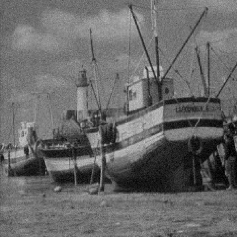
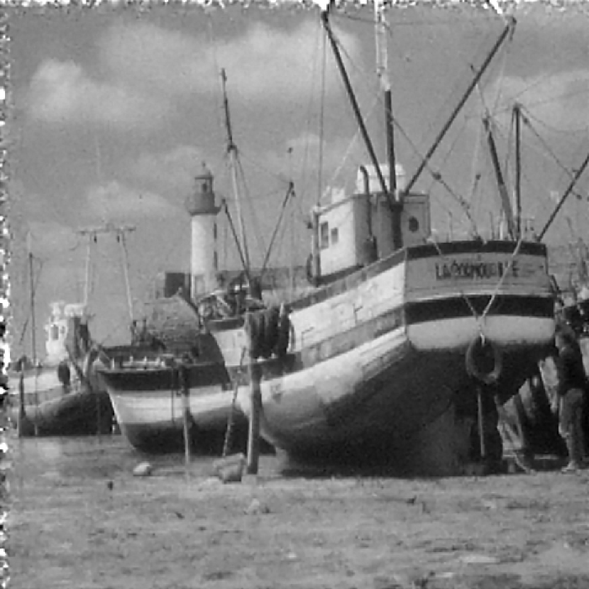
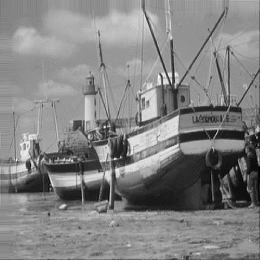
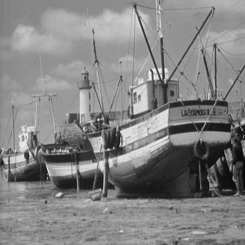
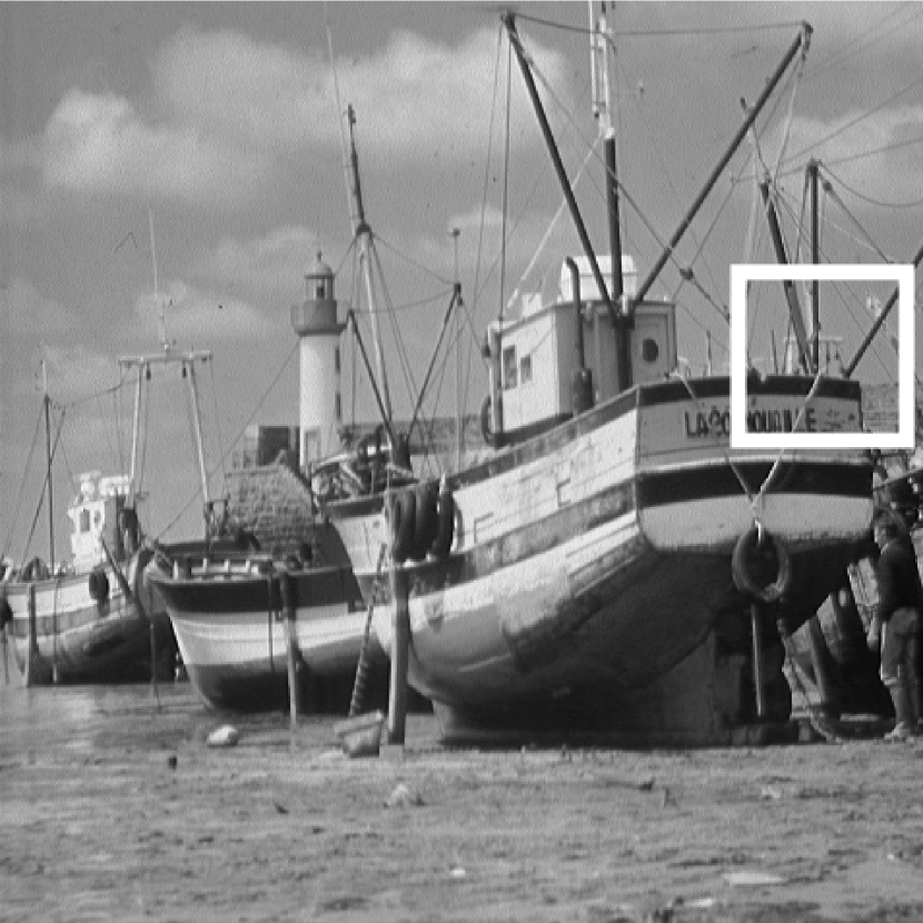
We start from a given HR image $\mathbf{f}^{*}$, see e.g. the boat image in Fig. 3(f). We translate and rotate $\mathbf{f}^{*}$ with known parameters and also change their illuminations by different scales. Then we downsample these frames with the given factor $r=2$ or $r=4$ to get our LR frames $\{\mathbf{g}_{i}\}_{i=1}^{p}$. We take $p=17$, and Gaussian noise of ratio 5% is added to each LR frame.

After we reconstruct the HR image $\mathbf{f}$ by a method, we compare it with the true solution $\mathbf{f}^{*}$ using two popular error measurements. The first one is peak signal-to-noise ratio (PSNR) and the second one is structural similarity (SSIM) [30]. For two signals $\mathbf{x}=(x_{1},x_{2},\cdots,x_{n})^{T}$ and $\mathbf{y}=(y_{1},y_{2},\cdots,y_{n})^{T}$, they are defined by

$$\text{PSNR}(\mathbf{x},\mathbf{y})=10\log_{10}\left(\frac{d^{2}}{\|\mathbf{x}-\mathbf{y}\|^{2}/n}\right),$$

$$\text{SSIM}(\mathbf{x},\mathbf{y})=\frac{(2\mu_{x}\mu_{y}+c_{1})(2\sigma_{xy}+c_{2})}{(\mu_{x}^{2}+\mu_{y}^{2}+c_{1})(\sigma_{x}^{2}+\sigma_{y}^{2}+c_{2})},$$

where $d$ is the dynamic range of $\mathbf{x},\mathbf{y}$ and $\mu_{x},\mu_{y}$ are the mean values of $\mathbf{x}$ and $\mathbf{y}$; $\sigma_{x},\sigma_{y}$ are the variances of $\mathbf{x}$ and $\mathbf{y}$; $\sigma_{xy}$ is the covariance of $\mathbf{x}$ and $\mathbf{y}$; $c_{i},i=1,2$ are constants related to $d$, which are typically set to be $c_{1}=(0.01d)^{2},c_{2}=(0.03d)^{2}$. Because of the motions, we do not have enough information to reconstruct $\mathbf{f}$ near the boundary; hence this part of $\mathbf{f}$ will not be accurate. Thus we restrict the comparison within the overlapping area of all LR images.

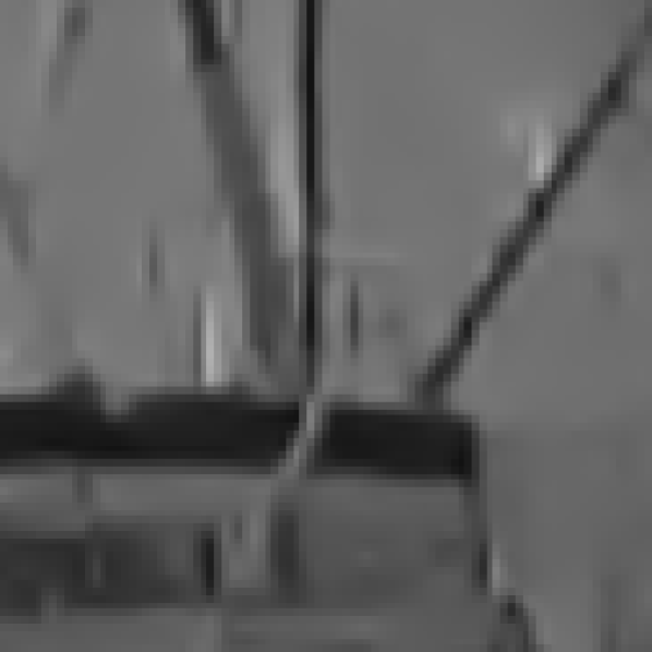
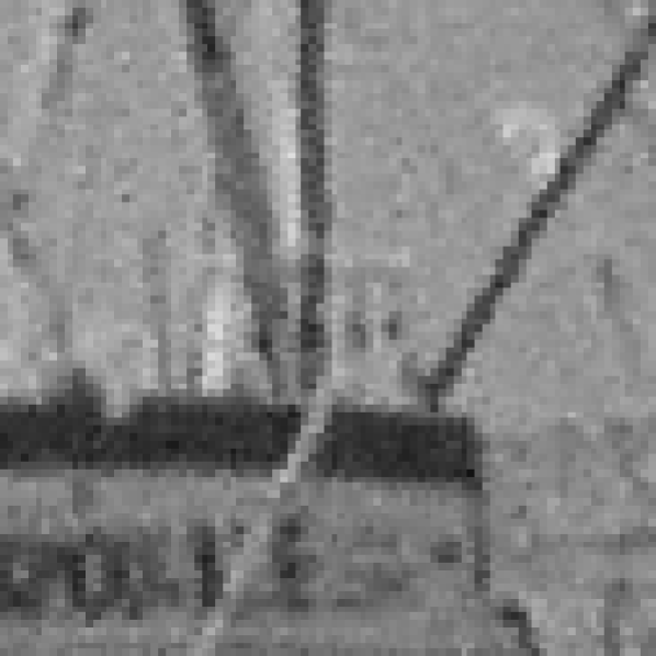
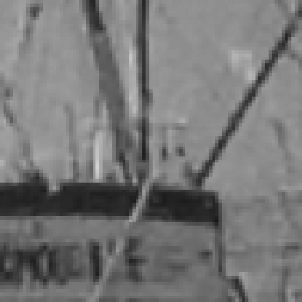
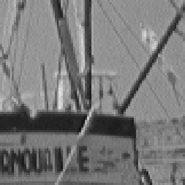
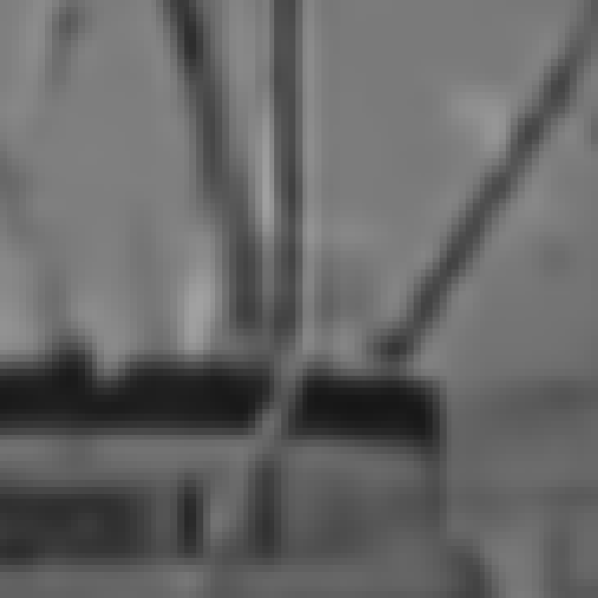
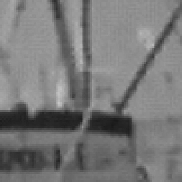
Table II gives the PSNR values and SSIM values of the reconstructed HR images $\mathbf{f}$ from the boat and the bridge videos. The results show that our model gives much more accurate $\mathbf{f}$ for both upsampling factor $r=2$ and $4$, see the boldfaced values there. The improvement is significant when comparing to the other three models, e.g. at least 1.6dB in PSNR for the boat video when $r=2$. From Table I, we also see that our method is the fastest. To compare the images visually, we give the results and their zoom-ins for the boat video in Figs. 3–5. The results for the bridge video are similar and therefore omitted. Fig. 3 shows the boat reconstructions for $r=2$. We notice that the TF model loses many fine details, e.g., the ropes of the mast. The MAP model produces some distortion on the edges and is sensitive to the noise; and the SDR model contains some artifacts along the edges. One can see the difference more clearly from the zoom-in images in Fig. 4. We also give the zoom-in results for $r=4$ in Fig. 5. We can see that the nuclear model produces more details and less artifacts than the other three models.

TABLE II: PSNR and SSIM values for the “Boat” and “Bridge” videos.

		Upsampling factor $r=2$				Upsampling factor $r=4$
		TF	MAP	SDR	Nuclear	TF	MAP	SDR	Nuclear
Boat	PSNR	18.7	25.3	28.2	29.8	20.7	23.6	27.0	27.5
	SSIM	0.69	0.70	0.80	0.83	0.69	0.67	0.72	0.77
Bridge	PSNR	20.7	23.6	27.0	27.5	20.1	22.4	24.1	25.0
	SSIM	0.69	0.67	0.72	0.77	0.53	0.57	0.65	0.72

(a) Reference LR image

(b) TF

(c) MAP

(d) SDR

(e) Nuclear

(f) True HR image

Figure 3: Comparison of different algorithms on “Boat” image with upsampling factor $r=2$. (a) The reference LR image. (b) Result of the TF model [6]. (c) Result of the MAP model [12]. (d) Result of the SDR model [17]. (e) Result of our nuclear model ($\lambda=1,\rho=400$). (f) True HR image.

(a) Original HR image

(b) TF

(c) MAP

(d) SDR

(e) Nuclear

(f) True HR image

Figure 4: Zoomed-in comparison of different algorithms on “Boat” image for $r=2$. (a) The zoom-in part in the HR image. (b) Result of the TF model [6]. (c) Result of the MAP model [12]. (d) Result of the SDR model [17]. (e) Result of our nuclear model ($\lambda=1,\rho=400$). (f) Zoomed-in original HR image.

(a) Reference LR image

(b) TF

(c) MAP

(d) SDR

(e) Nuclear

(f) True HR image

Figure 5: Zoom-in comparison of different algorithms on “Boat” image for $r=4$. (a) The reference LR image. (b) Result of the TF model [6]. (c) Result of the MAP model [12]. (d) Result of the SDR model [17]. (e) Result of our nuclear model ($\lambda=1,\rho=400$). (f) Zoomed-in original HR image.

IV-B Real videos

In the following, experiments on real videos are carried out. Four videos “Text”, “Disk”, “Alpaca” and “Eia” are downloaded from the website:

https://users.soe.ucsc.edu/~milanfar/software/sr-datasets.html.

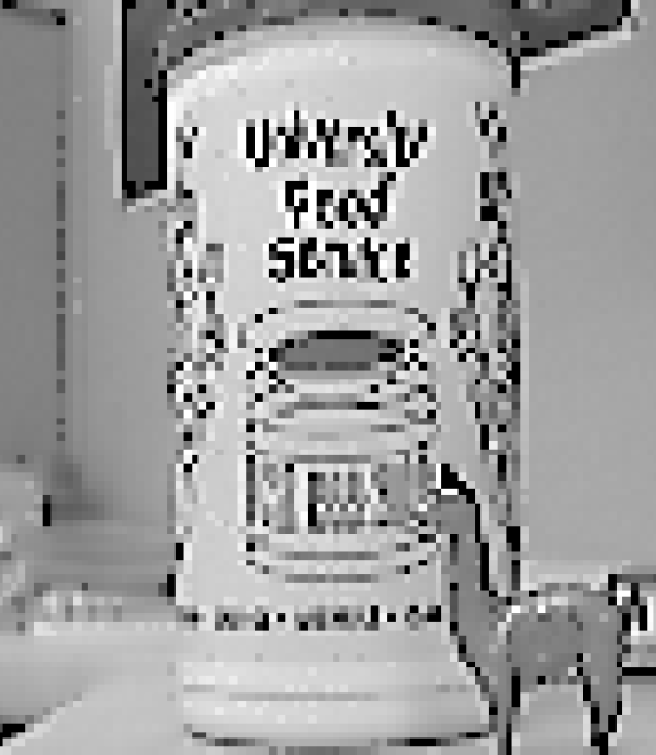
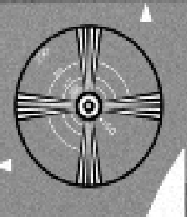
The basic information of these videos are listed in Table I. We see that they are very low-resolution videos. Fig. 6 shows the reference LR images for these videos. It is difficult to discern most of the letters from the reference images.

(a) Text

(b) Disk

(c) Alpaca

(d) Eia

Figure 6: The reference LR images of (a) “Text”, (b) “Disk”, (c) “Alpaca”, and (d) “Eia”.

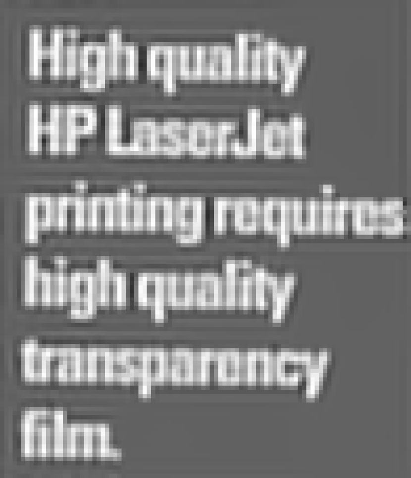
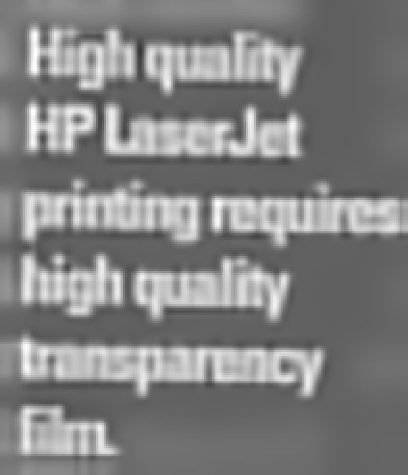
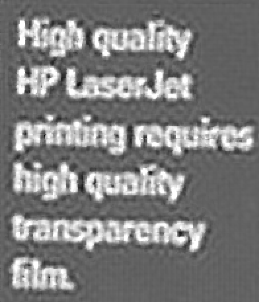
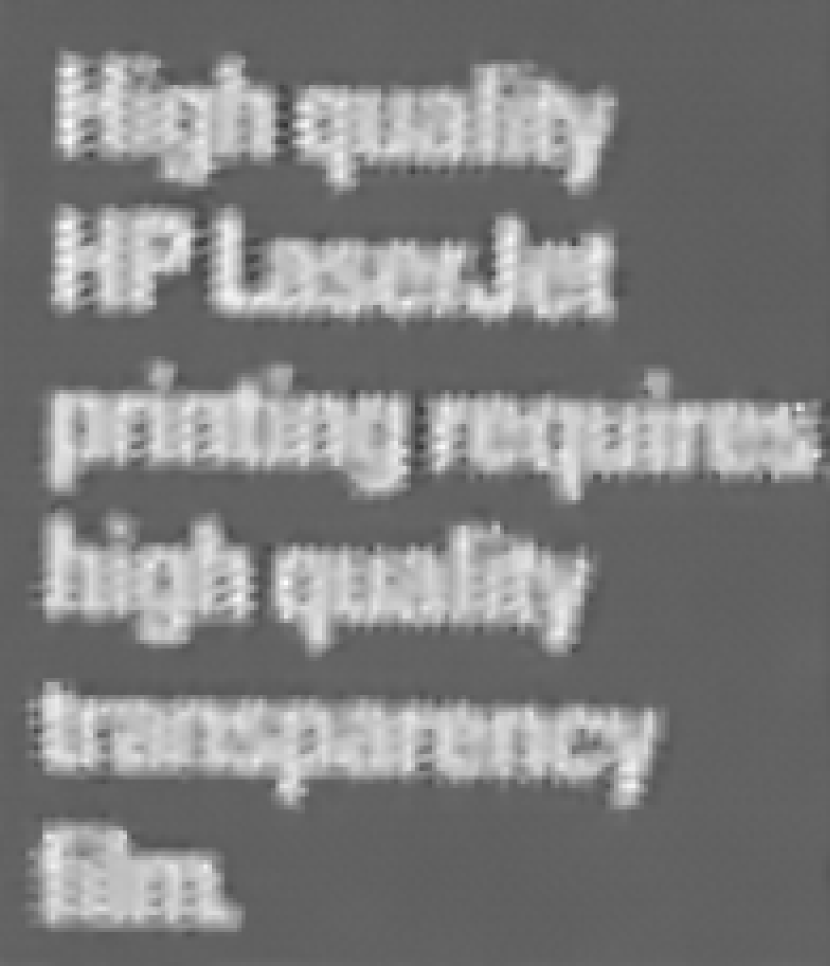
The first test video is the “Text Video”. The results are shown in Fig. 7. We see that the TF model produces blurry reconstructions. The images by the MAP model have obvious distortions. We also see that for the SDR model, some of the letters are coalesced, e.g. the word “film”. The results of the nuclear model is better. One can easily tell each word and there are no obvious artifacts for the letters.

(a) TF

(b) MAP

(c) SDR

(d) Nuclear

Figure 7: Comparison of different algorithms on “Text Video”. Top row with upsampling factor $r=2$ and second row with $r=4$. (a) Result of the TF model [6]. (b) Result of the MAP model [12]. (d) Result of the SDR model [17]. (d) Result of our nuclear model ($\lambda=1.5,\rho=50$ for $r=2$ and $\lambda=1.375,\rho=60$ for $r=4$).

The second video is the “Disk Video”, which contains 26 gray-scale images with the last 7 ones being zoom-in images. So we only use the first 19 frames in our experiment. The results are shown in Fig. 8. The TF model again produces blurry reconstructions. The MAP results are better but still blurry. The SDR results have some artifacts especially in the word “DIFFERENCE”. Our results are the best ones with each letter being well reconstructed, especially when $r=2$.

(a) TF

(b) MAP

(c) SDR

(d) Nuclear

Figure 8: Comparison of different algorithms on “Disk Video”. Top row with upsampling factor $r=2$ and second row with $r=4$. (a) Result of the TF model [6]. (b) Result of the MAP model [12]. (c) Result of the SDR model [17]. (d) Result of our nuclear model ($\lambda=1.125,\rho=50$ for both $r=2$ and $4$).

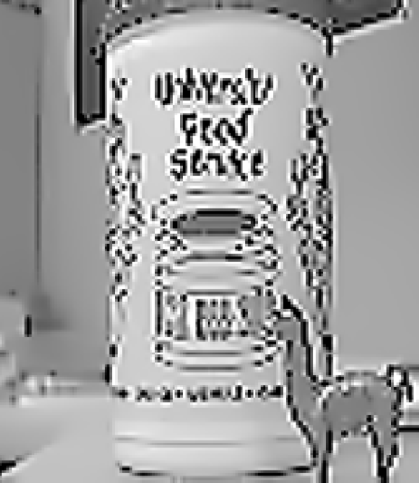
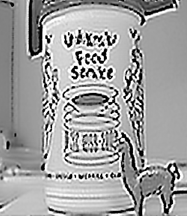
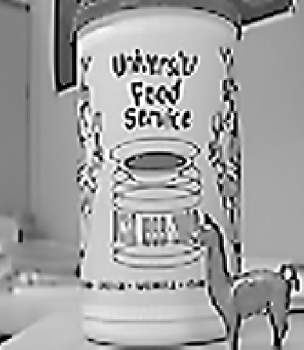
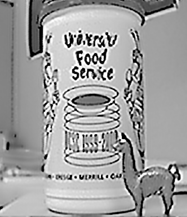
The third video is the “Alpaca Video”, and the results are shown in Fig. 9. When $r=2$, the word “Service” are not clear from the TF model, the MAP model and the SDR model. When $r=4$, the resulting images from all models are improved and the phrase “University Food Service” is clearer. However we can see that our nuclear model still gives the best reconstruction.

(a) TF

(b) MAP

(c) SDR

(d) Nuclear

Figure 9: Comparison of different algorithms on “Alpaca Video”. Top row with upsampling factor $r=2$ and second row with $r=4$. (a) Result of the TF model [6]. (b) Result of the MAP model [12]. (c) Result of the SDR model [17]. (d) Result of our nuclear model ($\lambda=1,\rho=50$ for $r=2$ and $\lambda=0.8,\rho=50$ for $r=4$).

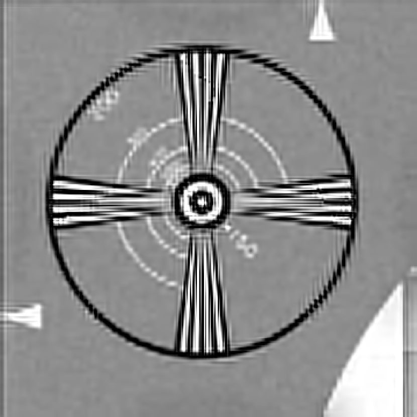
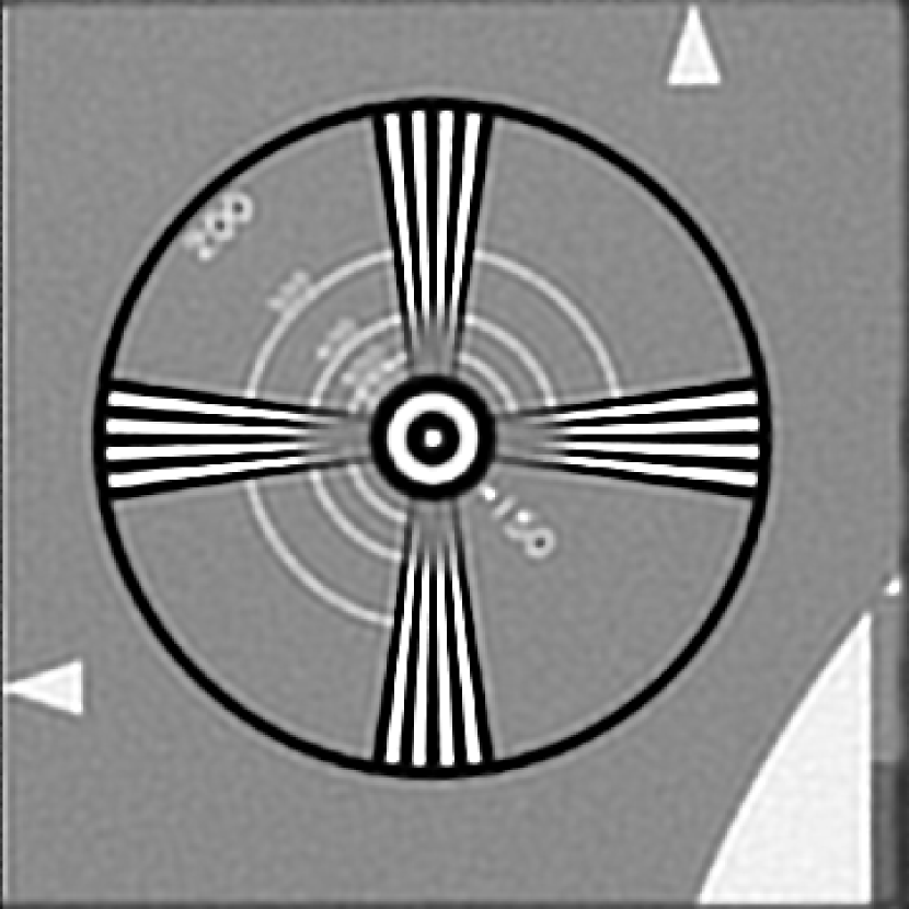
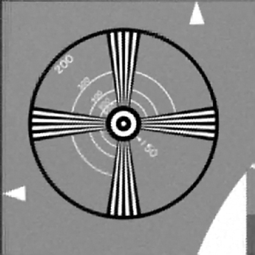
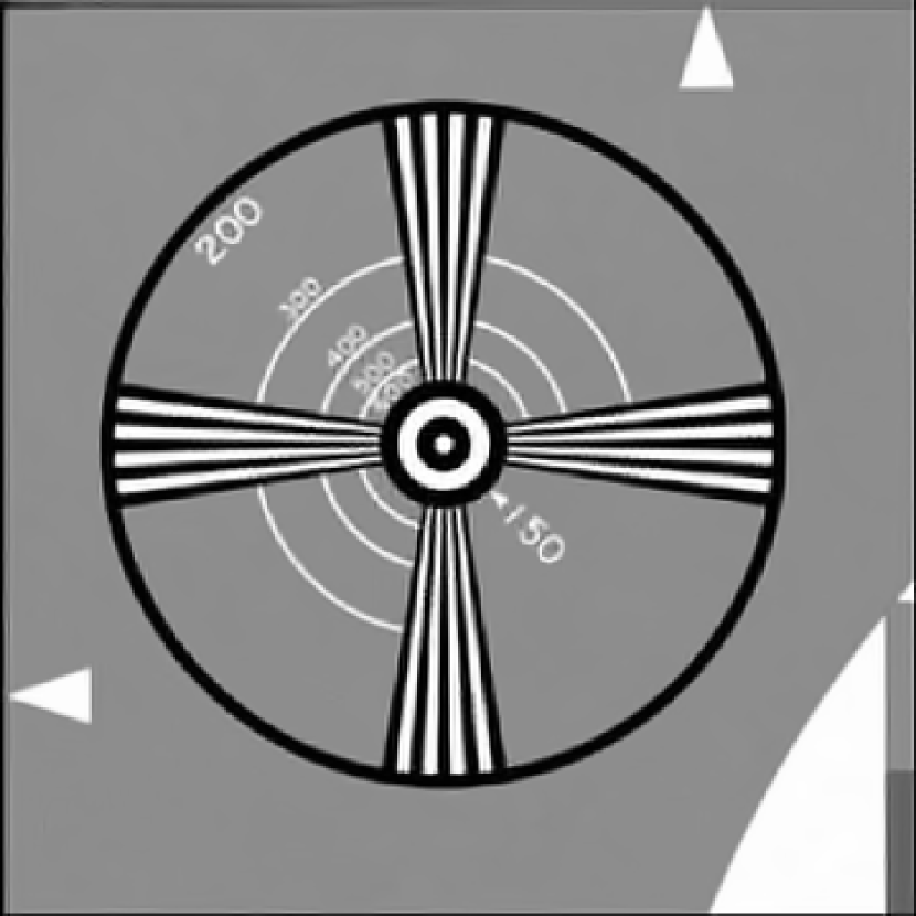
The fourth video is the “Eia Video” which show a testing image. There are some concentric circles labeled with different numbers in decreasing sizes. The results for $r=4$ are shown in Fig. 10. Our method gives an image where one can discern the number up to "500" with almost no artifacts while all the other methods can discern up to "200" at best with some noise or edge artifacts. This example clearly demonstrates the effectiveness of our model in MFSR.

(a) TF

(b) MAP

(c) SDR

(d) Nuclear

Figure 10: Comparison of different algorithms on “Eia Video” with upsampling factor $r=4$. (a) Result of the TF model [6]. (b) Result of the MAP model [12]. (c) Result of the SDR model [17]. (d) Result of our nuclear model ($\lambda=1,\rho=50$).

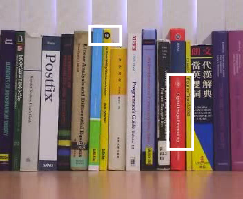
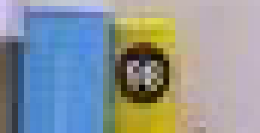
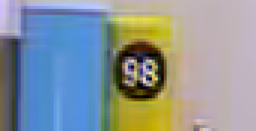
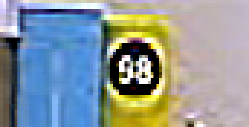
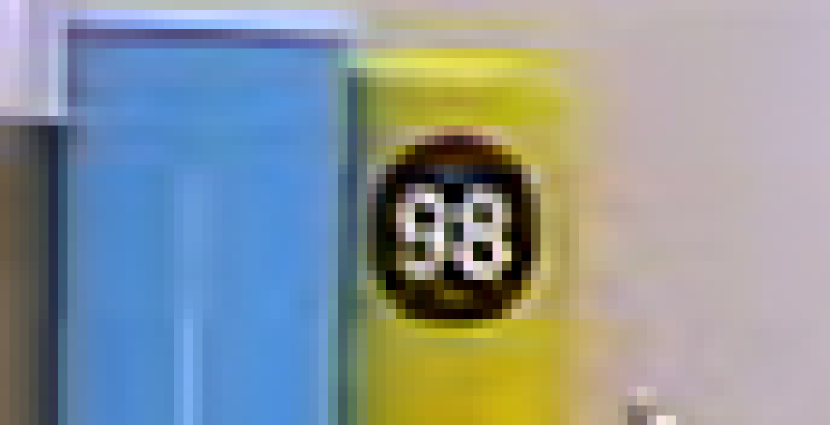
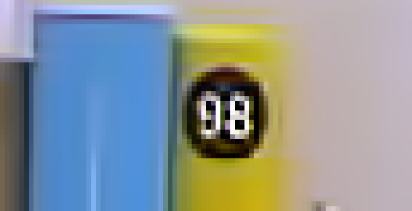
The last video is a color video which is used in the tests in [14, 6]. It contains $257$ color frames. We take the $100$-th frame to be the reference frame, see the leftmost figure in Fig. 11. Frame $90$ to frame $110$ in the video are used as LR images to enhance the reference image. We transform the RGB images into the Ycbcr color space, and then apply the algorithms to each color channel. Then we transform the resulting HR images back to the RGB color space. Figs. 11 and 12 show the zoom-in patches of the resulting images by different models. In Fig. 11, the patch shows a number “98” on the spine of a book. We see that the TF model gives a reasonable result when compared with MAP and SDR. However, our nuclear model gives the clearest “98” with very clean background. Fig. 12 shows the spines of two other books: “Fourier Transforms” and “Digital Image Processing”. Again, we see that our nuclear model gives the best reconstruction of the words with much less noisy artifacts.

(a) Zoomed-in LR

(b) TF

(c) MAP

(d) SDR

(e) Nuclear

Figure 11: Zoom-in comparison of different algorithms on “Books Video” with $r=2$. Left-most figure: the LR reference frame with zoom-in areas marked. (a) Zoomed-in LR image. (b) Result of the TF model [6]. (c) Result of the MAP model [12]. (d) Result of the SDR model [17]. (e) Result of our nuclear model ($\lambda=1.375,\rho=400$).

(a) Zoomed-in LR

(b) TF

(c) MAP

(d) SDR

(e) Nuclear

Figure 12: Another zoom-in comparison on “Books Video”with $r=2$. (a) Zoomed-in LR image. (b) Result of the TF model [6]. (c) Result of the MAP model [12]. (d) Result of the SDR model [17]. (e) Result of our nuclear model ($\lambda=1.375,\rho=400$).

V Conclusion

In this paper, we proposed an effective algorithm to reconstruct a high-resolution image using multiple low-resolution images from video clips. The LR images are first registered to the reference frame by using an optical flow. Then a low-rank model is used to reconstruct the high-resolution image by making use of the overlapping information between different LR images. Our model can handle complex motions and illumination changes. Tests on synthetic and real videos show that our model can reconstruct an HR image with much more details and less artifacts.

Rui Zhao received the B.S. degree in applied mathematics from Tsinghua University, Beijing, China in 2008, the M.S. degree in applied mathematics from Tsinghua University, Beijing, China in 2011. He is now a PhD student of Chinese University of Hong Kong. His main research area is image processing.

Raymond H. Chan is a SIAM Fellow and SIAM Council Member. He is Choh-Ming Li Professor of Chinese University of Hong Kong and Chairman of Department of Mathematicsis, Chinese University of Hong Kong. His research interests include numerical linear algebra and image processing problems.

References

- [1] R. Tsai and T. Huang, “Multiframe image restoration and registration,” Advances in computer vision and Image Processing, vol. 1, no. 2, pp. 317–339, 1984.
- [2] N. Bose and K. Boo, “High-resolution image reconstruction with multisensors,” International Journal of Imaging Systems and Technology, vol. 9, no. 4, pp. 294–304, 1998.
- [3] P. M. Shankar and M. A. Neifeld, “Sparsity constrained regularization for multiframe image restoration,” JOSA A, vol. 25, no. 5, pp. 1199–1214, 2008.
- [4] L. Shen and Q. Sun, “Biorthogonal wavelet system for high-resolution image reconstruction,” Signal Processing, IEEE Transactions on, vol. 52, no. 7, pp. 1997–2011, 2004.
- [5] S. Farsiu, M. Elad, and P. Milanfar, “Multiframe demosaicing and super-resolution of color images,” IEEE Transactions on Image Processing, vol. 15, no. 1, pp. 141–159, 2006.
- [6] R. H. Chan, Z. Shen, and T. Xia, “A framelet algorithm for enhancing video stills,” Applied and Computational Harmonic Analysis, vol. 23, no. 2, pp. 153–170, 2007.
- [7] Y. Lu, L. Shen, and Y. Xu, “Multi-parameter regularization methods for high-resolution image reconstruction with displacement errors,” Circuits and Systems I: Regular Papers, IEEE Transactions on, vol. 54, no. 8, pp. 1788–1799, 2007.
- [8] L. Duponchel, P. Milanfar, C. Ruckebusch, and J.-P. Huvenne, “Super-resolution and raman chemical imaging: From multiple low resolution images to a high resolution image,” analytica chimica acta, vol. 607, no. 2, pp. 168–175, 2008.
- [9] H. Takeda, P. Milanfar, M. Protter, and M. Elad, “Super-resolution without explicit subpixel motion estimation,” IEEE Transactions on Image Processing, vol. 18, no. 9, pp. 1958–1975, 2009.
- [10] C. M. Bishop, A. Blake, and B. Marthi, “Super-resolution enhancement of video,” in Proc. Artificial Intelligence and Statistics, vol. 2. Key West, FL, USA, 2003.
- [11] C. Liu and D. Sun, “On bayesian adaptive video super resolution,” Pattern Analysis and Machine Intelligence, IEEE Transactions on, vol. 36, no. 2, pp. 346–360, 2014.
- [12] Z. Ma, R. Liao, X. Tao, L. Xu, J. Jia, and E. Wu, “Handling motion blur in multi-frame super-resolution,” in 2015 IEEE Conference on Computer Vision and Pattern Recognition (CVPR), June 2015, pp. 5224–5232.
- [13] R. H. Chan, T. F. Chan, L. Shen, and Z. Shen, “Wavelet algorithms for high-resolution image reconstruction,” SIAM Journal on Scientific Computing, vol. 24, no. 4, pp. 1408–1432, 2003.
- [14] R. H. Chan, S. D. Riemenschneider, L. Shen, and Z. Shen, “Tight frame: an efficient way for high-resolution image reconstruction,” Applied and Computational Harmonic Analysis, vol. 17, no. 1, pp. 91–115, 2004.
- [15] L. I. Rudin, S. Osher, and E. Fatemi, “Nonlinear total variation based noise removal algorithms,” Physica D: Nonlinear Phenomena, vol. 60, no. 1, pp. 259–268, 1992.
- [16] S. Farsiu, M. D. Robinson, M. Elad, and P. Milanfar, “Fast and robust multiframe super resolution,” Image processing, IEEE Transactions on, vol. 13, no. 10, pp. 1327–1344, 2004.
- [17] Y.-R. Li, D.-Q. Dai, and L. Shen, “Multiframe super-resolution reconstruction using sparse directional regularization,” Circuits and Systems for Video Technology, IEEE Transactions on, vol. 20, no. 7, pp. 945–956, 2010.
- [18] X. Chen and C. Qi, “A single-image super-resolution method via low-rank matrix recovery and nonlinear mappings,” in Image Processing (ICIP), 2013 20th IEEE International Conference on, Sept 2013, pp. 635–639.
- [19] C. Jin, N. Y. J., and A. A., “Video super-resolution using low rank matrix completion,” Image Processing (ICIP), 2013 20th IEEE International Conference on, 2013.
- [20] Y. Altunbasak, A. Patti, and R. Mersereau, “Super-resolution still and video reconstruction from mpeg-coded video,” Circuits and Systems for Video Technology, IEEE Transactions on, vol. 12, no. 4, pp. 217–226, Apr 2002.
- [21] C. Wang, P. Xue, and W. Lin, “Improved super-resolution reconstruction from video,” Circuits and Systems for Video Technology, IEEE Transactions on, vol. 16, no. 11, pp. 1411–1422, 2006.
- [22] B. Narayanan, R. C. Hardie, K. E. Barner, and M. Shao, “A computationally efficient super-resolution algorithm for video processing using partition filters,” Circuits and Systems for Video Technology, IEEE Transactions on, vol. 17, no. 5, pp. 621–634, 2007.
- [23] M. V. W. Zibetti and J. Mayer, “A robust and computationally efficient simultaneous super-resolution scheme for image sequences,” Circuits and Systems for Video Technology, IEEE Transactions on, vol. 17, no. 10, pp. 1288–1300, 2007.
- [24] C. Gilliam and T. Blu, “Local all-pass filters for optical flow estimation,” in IEEE International Conference on Acoustics, Speech and Signal Processing, 2015.
- [25] E. J. Candès, X. Li, Y. Ma, and J. Wright, “Robust principal component analysis?” Journal of the ACM (JACM), vol. 58, no. 3, p. 11, 2011.
- [26] S. Boyd, N. Parikh, E. Chu, B. Peleato, and J. Eckstein, “Distributed optimization and statistical learning via the alternating direction method of multipliers,” Foundations and Trends® in Machine Learning, vol. 3, no. 1, pp. 1–122, 2011.
- [27] M. K. Ng, R. H. Chan, and W.-C. Tang, “A fast algorithm for deblurring models with neumann boundary conditions,” SIAM Journal on Scientific Computing, vol. 21, no. 3, pp. 851–866, 1999.
- [28] P. Thevenaz, U. E. Ruttimann, and M. Unser, “A pyramid approach to subpixel registration based on intensity,” Image Processing, IEEE Transactions on, vol. 7, no. 1, pp. 27–41, 1998.
- [29] C. Liu, “Beyond pixels: exploring new representations and applications for motion analysis,” Ph.D. dissertation, Citeseer, 2009.
- [30] Z. Wang, A. C. Bovik, H. R. Sheikh, and E. P. Simoncelli, “Image quality assessment: from error visibility to structural similarity,” IEEE Transactions on Image Processing, vol. 13, no. 4, pp. 600–612, April 2004.