Understanding the Mechanisms of Deep Transfer Learning for Medical Images
Abstract
The ability to automatically learn task specific feature representations has led to a huge success of deep learning methods. When large training data is scarce, such as in medical imaging problems, transfer learning has been very effective. In this paper, we systematically investigate the process of transferring a Convolutional Neural Network, trained on ImageNet images to perform image classification, to kidney detection problem in ultrasound images. We study how the detection performance depends on the extent of transfer. We show that a transferred and tuned CNN can outperform a state-of-the-art feature engineered pipeline and a hybridization of these two techniques achieves 20% higher performance. We also investigate how the evolution of intermediate response images from our network. Finally, we compare these responses to state-of-the-art image processing filters in order to gain greater insight into how transfer learning is able to effectively manage widely varying imaging regimes.
1 Introduction
Automated organ localization and segmentation from ultrasound images is a challenging problem because of specular noise, low soft tissue contrast and wide variability of data from patient to patient. In such difficult problem settings, data driven machine learning methods, and especially deep learning methods in recent times, have found quite a bit of success. Usually, a large amount of labeled data is needed to train machine learning models and a careful feature engineering is required for each problem. The question of how much data is needed for satisfactory performance of these methods is still unanswered, with some recent works in this direction [7]. However, transfer learning has been successfully employed in data scarce situations, with model knowledge being effectively transferred across (possibly unrelated) tasks/domains. It is fascinating that a model, learnt for an unrelated problem setting can actually solve a problem at hand with minimal retraining. In this paper, we have attempted to demonstrate and understand the effectiveness and mechanism of transfer learning a CNN, originally learnt on camera images for image recognition, to solve the problem of automated kidney localization from ultrasound B-mode images.
Kidney detection is challenging due to wide variability in its shape, size and orientation. Depending upon the acquisition scan plane, inconsistency in appearance of internal regions (renal sinus) and presence of adjacent structures like diaphragm, liver boundaries, etc. pose additional challenges. This is also a clinically relevant problem as kidney morphology measurements are essential in assessing renal abnormalities [13], planning and monitoring radiation therapy, and renal transplant.
There have been semi-automated and automated kidney detection approaches reported in literature. In [22], a texture model is built by an expectation maximization algorithm using features inferred from a bank of Gabor filters, followed by iterative segmentation to combine texture measures into parametric shape model. In [16], Markov random fields and active contour methods have been used to detect kidney boundaries in 3D ultrasound images. Recently, machine learning approaches [1, 17] based on kidney texture analysis have proven successful for segmentation of kidney regions from 2-D and 3-D ultrasound images.
2 State of the art
CNNs [15] provide effective models for vision learning tasks by incorporating spatial context and weight sharing between pixels. A typical deep CNN for a learning task has, as input, channel image patches of size , where , . The output is feature maps, , defined as convolutions using filters , of size , and scalars . We then have:
| (1) |
Here, denotes convolution, is a non-linear function (sigmoid or a linear cutoff (ReLU)). is a down sampling operator. The number of feature maps, filter size, and size of the feature maps are hyperparameters in the above expression, with a total of parameters that one has to optimize for a learning task. A deep CNN architecture is multi-layered, with the above expression being hierarchically stitched together, given the number of input/output maps, sizes of filters and maps for each layer, resulting in a huge number of parameters to be optimized. When data is scarce, the learning problem is under-determined and therefore transferring CNN parameters from a pre-learned model helps.
For medical image problems, transfer learning is additionally attractive due to the heterogeneity of data types (modalities, anatomies, etc.) and clinical challenges. In [4], the authors perform breast image classification using a CNN model trained on ImageNet. Shie et al. [18] employ the CaffeNet, trained on ImageNet, to extract features and classify Otitis Media images. In [6], a pre-trained CNN is used to extract features on ultrasound images to localize a certain standard plane that is important for diagnosis.
Studies on transferability of features across CNNs include [23] and more specifically [19],[21] for medical images. While our work demonstrates yet another success of transfer learning for medical imaging and the tuning aspects of transfer learning, we
-
1.
Reason out the effectiveness of transfer learning by methodically comparing the response maps from various layers of transfer learnt network with traditional image processing filters.
-
2.
Investigate the effect of level of tuning on performance. We demonstrate that full network adaptation leads to learning problem specific features and also establishes the superiority over off-the-shelf image processing filters.
-
3.
Re-establish the relevance and complementary advantages of state-of-the-art, hand-crafted features and merits of hybridisation approaches with CNNs, to help us achieve next level performance improvement [24].
3 Methods
From a set of training images, we build classifiers to differentiate between kidney and non-kidney regions. On a test image, the maximum likelihood detection problem of finding the best kidney region of interest (ROI) from a set of candidate ROIs is split into two steps, similar to [3, 17]. The entire set is passed through our classifier models and the candidates with positive class labels () are retained (Eq. (2)). The ROI with highest likelihood () from the set is selected as the detected kidney region (Eq. (3))
| (2) |
| (3) |
We propose to employ CNNs as feature extractors similar to [10] to facilitate comparisons with traditional texture features. We also propose to use a well-known machine learning classifier, to evaluate performance of different feature sets, thereby eliminating the effects of having soft-max layer for CNNs and a different classifier on traditional features as our likelihood functions.
3.1 Dataset and Training
We considered a total of 90 long axis kidney images acquired on GE Healthcare LOGIQ E9 scanner, split into two equal and distinct sets, for training and validation. The images contained kidney of different sizes with lengths varying between 7.5cm and 14cm and widths varying between 3.5cm and 7cm, demonstrating wide variability in the dataset. The orientation of the kidneys varied between -25∘ and +15∘. The images were acquired at varying depths of ultrasound acquisition ranging between 9cm and 16cm. Accurate rectangular ground truth kidney ROIs were manually marked by a clinical expert.
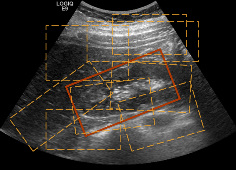
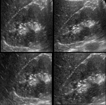
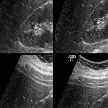
To build our binary classification models from training images, we swept the field of view (FOV) to generate many overlapping patches of varying sizes (see Fig. 1) that satisfied clinical guidelines on average adult kidney dimensions and aspect ratio [8]. We downsampled these ROIs to a common size and were further binned into two classes based on their overlap with ground truth annotations. We used Dice similarity coefficient (DSC) as the metric and a threshold of 0.8 (based on visual and clinical feedback) was used to generate positive and negative class samples. This was followed by feature extraction and model building.
3.2 Transfer Learned Features
Our study on transfer learning was based on adapting the popular CaffeNet [11] architecture built on ImageNet database to ultrasound kidney detection, whose simplified schematic is in Fig. 2. We extracted features after the ‘fc7’ layer from all the updated nets, resulting in 4096 features. The features extracted were:
-
1.
Full Network adaptation (CaffeNet_FA) - Initialized with weights from CaffeNet parameters, the entire network weights were updated by training on kidney image samples from Section 3.1. The experiment settings were: stochastic gradient descent update with a batch size of 100, momentum of 0.5 and weight decay of .
-
2.
Partial Network adaptation (CaffeNet_PA) - To understand the performance difference based on level of tuning, we froze the weights of ‘conv1’ and ‘conv2’ layers, while updating the weights of other layers. The reasoning behind freezing the first two layers was to evaluate how sharable were the low-level features and also to help us in interpret-ability (Sec. 5). The experiment settings were same as those for full network adaptation.
-
3.
Zero Network adaptation (CaffeNet_NA) - Finally, we also extracted features from the original CaffeNet model without modifying the weights.
3.3 Traditional Texture Features
3.4 Gradient Boosting Machine (GBM)
Ensemble classifiers have been shown to be successful in ultrasound organ detection problems. In [3], authors have used probabilistic boosting tree classifier for fetal anatomy detection. In [17], it has been noted that gradient boosting machine (GBM) have outperformed adaboost classfiers. In an empirical comparison study of supervised learning algorithms [5] comparing random forests and boosted decision trees, calibrated boosted trees had the best overall performance with random forests being close second. Motivated by these successes, we have chosen to use Gradient boosting tree as our classifier model. We build GBM classifiers for all the feature sets explained in Section 3.2 and 3.3 using GBM implementation inspired by [2], with parameters: shrinkage factor and sampling factor set to 0.5, maximum tree depth = 2 and number of iterations = 200.
3.5 Hybrid approach
Investigation of the failure modes of baseline method (Haar + GBM) and CaffeNet_FA revealed that they had failed on different images (Section 4). To exploit the complementary advantages, we propose a simple scheme of averaging the spatial likelihood maps from GBMs of these two approaches and employing it in (2), which yields dramatic improvement.

4 Results
To quantitatively evaluate the performance on 45 validation images, we used two metrics: (1) Number of localization failures - the number of images for which the dice similarity coefficient between detected kidney ROI and ground truth annotation was 0.80. (2) Detection accuracy - average dice overlap across 45 images between detection results and ground truth, which . From Table 1, we see that CaffeNet features without any adaptation outperformed baseline by 2% in average detection accuracy with same number of failures. This improvement is consistent with other results reported in literature [18], where CaffeNet features outperform state-of-the-art pipeline. However, by allowing these network weights to get adapted to the kidney data, we achieved a performance boost of 4% over the baseline method, with number of failure cases reducing to 10 from 12. Interestingly, tuning with the first two convolutional layers frozen yielded intermediate performance, suggesting that multiple levels of feature adaptation are important to the problem.
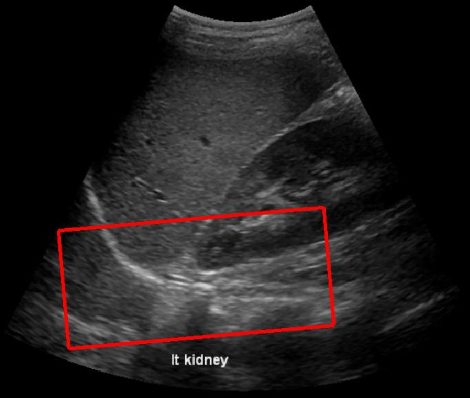
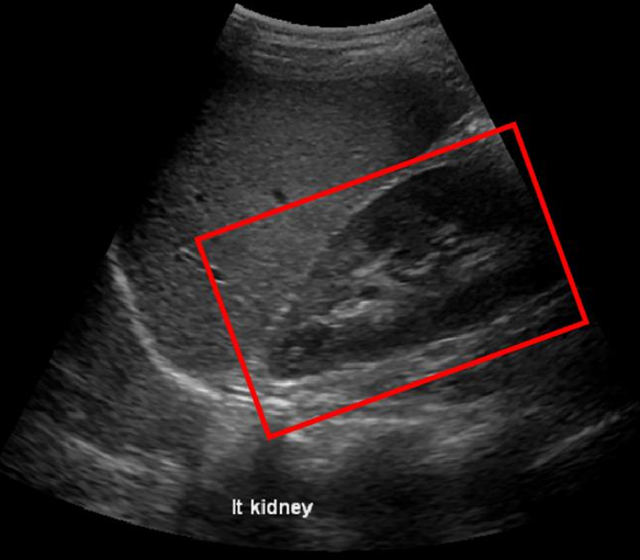
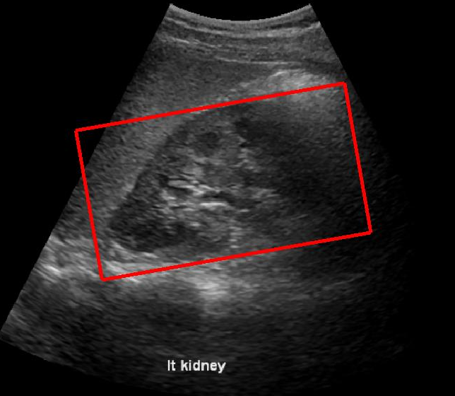
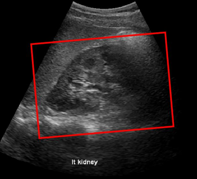
Fig. 3LABEL:sub@subfig:a and LABEL:sub@subfig:b shows a case in which the baseline method was affected by the presence of diaphragm, kidney and liver boundaries creating a texture similar to renal-sinus portion, while CaffeNet had excellent localization. Fig. 3LABEL:sub@subfig:c and LABEL:sub@subfig:d illustrate a case where CaffeNet resulted in over-segmentation containing the diaphragm, clearly illustrating that in limited data problems careful feature-engineering incorporating domain knowledge still carries a lot of relevance. Finally, we achieved a best performance of 86% average detection accuracy using the hybrid approach (Section 3.5). More importantly, the number of failures of the hybrid approach was 3/45, which is 20% better than either of the methods.
| Method | Haar Features | CaffeNet_NA | CaffeNet_PA | CaffeNet_FA | Haar + CaffeNet_FA |
|---|---|---|---|---|---|
| Average Dice overlap | 0.793 | 0.825 | 0.831 | 0.842 | 0.857 |
| # of failures | 12/45 | 12/45 | 11/45 | 10/45 | 3/45 |
5 Discussion
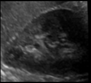
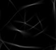
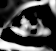
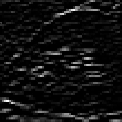
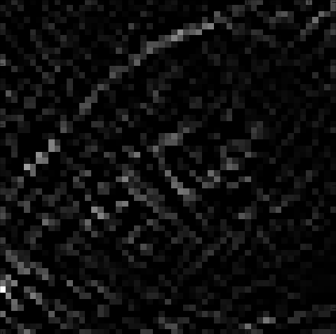
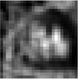
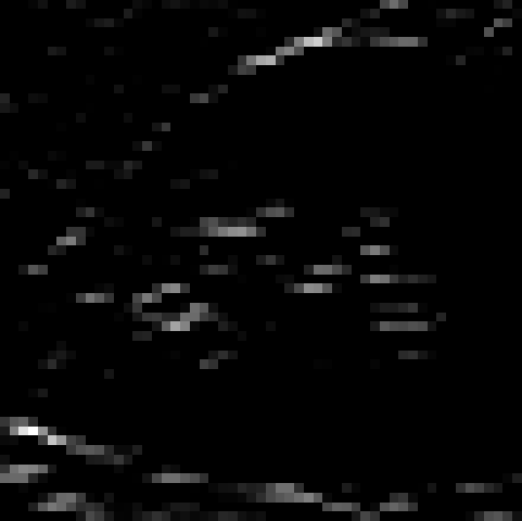
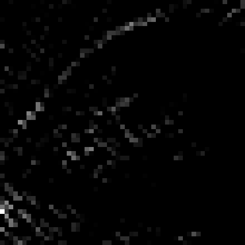
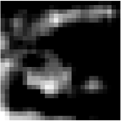
It is indeed very interesting to see that features learnt on camera images were able to outperform careful feature engineering on sharply different detection problems, in modalities whose acquisition physics are distinctly different. Fig. 4 compares some of the response images generated from layers 1 and 2 of the learned network with traditional image processing outputs like Phase Congruency [14] and Frangi vesselness filter [9] for an example patch.
Here, we would like to highlight two main points: (1) Visually, we find the output has intriguing similarities with the outputs of hand crafted feature extractors optimized for Ultrasound. The response maps of Fig. 4LABEL:sub@subfig:CNFA_L11 and LABEL:sub@subfig:CNFA_L2 are similar to 4LABEL:sub@subfig:PC and LABEL:sub@subfig:frangi. This is very encouraging because of the fact that CNNs learns features that are equivalent to some of these widely used non-linear feature extractors. (2) The second important observation here is the reduction in speckle noise on CaffeNet_FAL1_1, compared to CaffeNet_PAL1_1. By carefully tuning CaffetNet features on ultrasound data, the model was able to learn the underlying noise characteristics, while preserving edges, and this resulted in a much improved response map as shown in Fig. 4LABEL:sub@subfig:CNFA_L11 and LABEL:sub@subfig:CNFA_L2.
| Layer | |||||
|---|---|---|---|---|---|
| Conv1 | Conv2 | Conv3 | Conv4 | Conv5 | |
| # of filters with 40% change | 0 | 5 | 125 | 22 | 62 |
Further, we quantitatively analyzed changes (% in norm) in filter weights in each layer to identify significant trends. Table 2 shows a large number of filters have significantly changed in the 3rd layer, with filters in the 1st and 2nd layer showing minimal change. This is possibly due to the lower level features being fairly the same for both natural and ultrasound images. We also noted that the use of ReLU as the activation function also avoided the vanishing gradient problem, resulting in this skew in distribution of weight changes across layers. The response images past layer 2 proved to be difficult to interpret, and may require more intensive techniques. Our quantitative results and the literature in the field show that a great deal of the power of deep networks lies in these layers, and so we feel this is an important area for our future investigation.
In a clinical context, the interpretability of models is crucial and we feel this insight into why the deep CNN was able to outperform hand-crafted features is as important as the results demonstrated in Sec. 4. We also see this as opening up new ways of understanding and utilizing deep networks for medical problems.
References
- [1] Roberto Ardon, Remi Cuingnet, Ketan Bacchuwar, and Vincent Auvray. Fast kidney detection and segmentation with learned kernel convolution and model deformation in 3d ultrasound images. In Proc. of ISBI, pages 268–271, 2015.
- [2] Carlos Becker, Roberto Rigamonti, Vincent Lepetit, and Pascal Fua. Supervised feature learning for curvilinear structure segmentation. In Proc. of MICCAI 2013, pages 526–533, 2013.
- [3] G. Carneiro, B. Georgescu, S. Good, and D. Comaniciu. Detection and measurement of fetal anatomies from ultrasound images using a constrained probabilistic boosting tree. IEEE Trans. on Med. Imag., 27(9):1342–1355, Sept 2008.
- [4] Gustavo Carneiro, Jacinto Nascimento, and Andrew P. Bradley. Unregistered multiview mammogram analysis with pre-trained deep learning models. In Proc. of MICCAI, pages 652–660, 2015.
- [5] Rich Caruana and Alexandru Niculescu-Mizil. An empirical comparison of supervised learning algorithms. In Proc. of ICML, pages 161–168, 2006.
- [6] H. Chen, D. Ni, J. Qin, S. Li, X. Yang, T. Wang, and P. A. Heng. Standard plane localization in fetal ultrasound via domain transferred deep neural networks. IEEE Journal of Biomedical and Health Informatics, 19(5):1627–1636, Sept 2015.
- [7] Junghwan Cho, Kyewook Lee, Ellie Shin, Garry Choy, and Synho Do. How much data is needed to train a medical image deep learning system to achieve necessary high accuracy? In ICLR, 2016.
- [8] S. A. Emamian, M. B. Nielsen, J. F. Pedersen, and L. Ytte. Kidney dimensions at sonography: correlation with age, sex, and habitus in 665 adult volunteers. American Journal of Roentgenology, 160(1):83–86, Jan 1993.
- [9] A. F. Frangi, W. J. Niessen, K. L. Vincken, and M. A. Viergever. Multiscale vessel enhancement filtering. In Proc. of MICCAI, pages 130–137, 1998.
- [10] Ross Girshick, Jeff Donahue, Trevor Darrell, and Jitendra Malik. Rich feature hierarchies for accurate object detection and semantic segmentation. 2014.
- [11] Yangqing Jia, Evan Shelhamer, Jeff Donahue, Sergey Karayev, Jonathan Long, Ross Girshick, Sergio Guadarrama, and Trevor Darrell. Caffe: Convolutional architecture for fast feature embedding. In Proc. of the ACM Int. Conf. on Multimedia, pages 675–678, 2014.
- [12] Eystratios G. Keramidas, Dimitris K. Iakovidis, Dimitris Maroulis, and Stavros Karkanis. Efficient and effective ultrasound image analysis scheme for thyroid nodule detection. In Proc. of ICIAR, pages 1052–1060, 2007.
- [13] Arpana M. Kop and Ravindra Hegadi. Kidney segmentation from ultrasound images using gradient vector force. IJCA, Special Issue on RTIPPR, 2:104–109, 2010.
- [14] Peter Kovesi. Phase congruency detects corners and edges. In Proc. of The Australian Pattern Recognition Society Conference: DICTA, pages 309–318, 2003.
- [15] Alex Krizhevsky, Ilya Sutskever, and Geoffrey E. Hinton. Imagenet classification with deep convolutional neural networks. In Proc. of Adv. in NIPS, pages 1106–1114, 2012.
- [16] Marcos Martin-Fernandez and Carlos Alberola-Lopez. An approach for contour detection of human kidneys from ultrasound images using markov random fields and active contours. Medical Image Analysis, 9(1):1 – 23, 2005.
- [17] H Ravishankar and Pavan Annangi. Automated kidney morphology measurements from ultrasound images using texture and edge analysis. In SPIE Med. Imag., 2016.
- [18] Chuen-Kai Shie, Chung-Hisang Chuang, Chun-Nan Chou, Meng-Hsi Wu, and E. Y. Chang. Transfer representation learning for medical image analysis. In EMBC, pages 711–714, 2015.
- [19] Hoo-Chang Shin, Holger R. Roth, Mingchen Gao, Le Lu, Ziyue Xu, Isabella Nogues, Jianhua Yao, Daniel J. Mollura, and Ronald M. Summers. Deep convolutional neural networks for computer-aided detection: CNN architectures, dataset characteristics and transfer learning. IEEE Trans. Med. Imaging, 35(5):1285–1298, 2016.
- [20] A. S. M. Sohail, M. M. Rahman, P. Bhattacharya, S. Krishnamurthy, and S. P. Mudur. Retrieval and classification of ultrasound images of ovarian cysts combining texture features and histogram moments. In Proc. of ISBI, pages 288–291, April 2010.
- [21] Nima Tajbakhsh, Jae Y. Shin, Suryakanth R. Gurudu, R. Todd Hurst, Christopher B. Kendall, Michael B. Gotway, and Jianming Liang. Convolutional neural networks for medical image analysis: Full training or fine tuning? IEEE Trans. Med. Imaging, 35(5):1299–1312, 2016.
- [22] Jun Xie, Yifeng Jiang, and Hung-Tat Tsui. Segmentation of kidney from ultrasound images based on texture and shape priors. IEEE Trans. on Med. Imag., 24(1):45–57, 2005.
- [23] Jason Yosinski, Jeff Clune, Yoshua Bengio, and Hod Lipson. How transferable are features in deep neural networks? In Proc. of Adv. in NIPS, pages 3320–3328, 2014.
- [24] Yefeng Zheng, David Liu, Bogdan Georgescu, Hien Nguyen, and Dorin Comaniciu. 3d deep learning for efficient and robust landmark detection in volumetric data. In Proc. of MICCAI, pages 565–572, 2015.