Unsupervised Construction of Human Body Models Using Principles of Organic Computing

Abstract

Unsupervised learning of a generalizable model of the visual appearance of humans from video data is of major importance for computing systems interacting naturally with their users and others. We propose a step towards automatic behavior understanding by integrating principles of Organic Computing into the posture estimation cycle, thereby relegating the need for human intervention while simultaneously raising the level of system autonomy. The system extracts coherent motion from moving upper bodies and autonomously decides about limbs and their possible spatial relationships. The models from many videos are integrated into meta-models, which show good generalization to different individuals, backgrounds, and attire. These models allow robust interpretation of single video frames without temporal continuity and posture mimicking by an android robot.

I Introduction

Humans show unmatched expertise in analyzing and interpreting body movement and anticipating intentions and future behavior. This skill of social perception is one of the foundations of effective and smooth interaction of humans inhabiting a complex environment. The benefits of machines capable of interpreting human motion would be enormous: applications in health care, surveillance, industry and sports (Gavrila, 1999; Moeslund et al., 2006) promise a broad market. Despite significant effort (Poppe, 2007) to transfer human abilities in motion estimation and behavioral interpretation to synthetic systems, automatically looking at people (Gavrila, 1999) remains among the ‘most difficult recognition problem[s] in computer vision’ (Mori et al., 2004) there is no technical solution matching human competency in vision-based motion capturing (VBMC).

Artificial VBMC systems should be enhanced by learning lessons from human perception. To that end, we have pursued an organic computing (OC) (von der Malsburg, 2008) approach and introduce cerebral information processing paradigms (including self-organization, self-optimization, concept building, generalization, and non-trivial learning (Poggio and Bizzi, 2004) into vision-based human posture analysis. The resulting system is able to acquire conceptual models of the upper human body in a completely autonomous manner: the learning procedures are based on only a few general principles. This strategy significantly reduces human workload and allows self-optimization of the generated models. While autonomous model learning and knowledge agglomeration take place in simple scenarios, the conceptual nature of the retrieved body representations allows for generalization to more complex scenarios and holds opportunities for model adaptation and enhancement loops, which might perform continuous, non-trivial learning as found in the human brain.

\begin{overpic}[height=480.59395pt]{Images/fig_SystemOverview/SystemOverview.jpg} \put(50.0,97.2){\Large\sf(a)} \put(44.0,79.2){\sf(b)} \put(14.5,74.5){\scriptsize\sf(c)} \put(31.0,74.5){\scriptsize\sf(d)} \put(45.0,74.5){\scriptsize\sf(e)} \put(61.0,74.5){\scriptsize\sf(f)} \put(39.0,69.6){\sf(g)} \put(42.0,64.6){\sf(h)} \put(20.0,44.8){\scriptsize\sf(i)} \put(36.0,44.8){\scriptsize\sf(j)} \put(51.5,44.8){\scriptsize\sf(k)} \put(20.0,30.1){\sf(l)} \put(36.5,26.2){\sf(m)} \put(52.0,30.1){\sf(n)} \put(33.0,14.8){\scriptsize\sf(o)} \put(42.0,6.7){\scriptsize\sf(p)} \put(45.0,1.9){\Large\sf(q)} \end{overpic}

Figure 1: Schematic overview of the proposed VBMC system: green regions indicate organic learning components, blue areas envelop standard bottom-up VBMC (cf. section II) components.

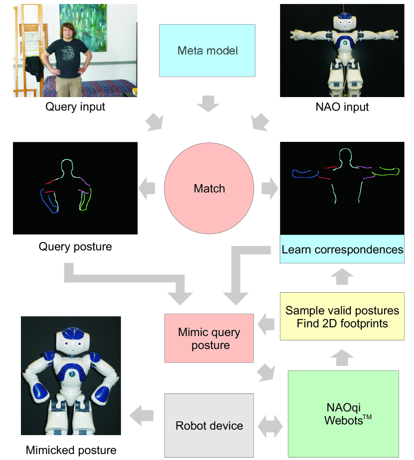
Fig. 1 provides a schematic overview of the system and is referred to throughout the paper for all components. In section II we give an overview of VBMC approaches that have been considered or used in this work and discuss their strenghts and weaknesses. Section III describes the details of learning a body model from a single video of human motion. In section V many such models are combined into a meta-model, which captures the invariant cues of the single models. Section 5 tests the learned meta-model on still images with different backgrounds, individuals, attire, etc. Relations with powerful supervised models are discussed. The paper closes with a short discussion.

II Previous work in vision-based human motion capturing

Following Poppe (2007), VBMC methods can be classified into model-based, generative approaches and model-free, discriminative methods (cf. also (Navaratnam et al., 2006)). Model-based schemes incorporate top-down and bottom-up techniques, while the model-free domain employs learning-based and exemplar-based pose estimation.

To stay in scope, we leave an in-depth discussion of top-down and discriminative techniques to Poppe (2007) or Walther (2011). Bottom-up solutions form an important mainstay of our own approach and are thus investigated more closely. Nevertheless, our focus is on autonomous, fully unsupervised VBMC strategies that try to enhance systemic autonomy and directly relate to the organically inspired posture estimation method proposed in this paper.

II-A Bottom-up posture estimation

A generic bottom-up (or combinatorial (Roberts et al., 2007)) posture estimation system follows the principle formulated in (Sigal and Black, 2006a): ‘measure locally, reason globally.’ Local measurement treats the human body as an ensemble of ‘quasi-independent’ (Sigal et al., 2003) limbs, which much alleviates the complex model coupling inherent in top-down approaches. Imposing independence, ‘image measurements’ (Sigal et al., 2003) of single limbs can be performed separately by a dedicated limb detector (LD) (Sigal and Black, 2006b; Ramanan et al., 2007), which moves the burden of matching a given body part model to some well-chosen image descriptors (Kanaujia et al., 2007; Poppe, 2007). The selection of appropriate images descriptors as well as construction and application of LDs require domain knowledge of and concept building by human supervisors. For many object categories, histograms of oriented gradient (HOG) features seem to be a good choice, allowing object classification by linear discriminant analysis (Hariharan et al., 2012).

To organize the data from local measurements, pending inter-limb dependencies come into play during global reasoning. ‘Assemblies’ (Moeslund et al., 2006) of detector responses are retrieved that comply well with kinematically meaningful human body configurations. The majority of bottom-up systems employ graphical models (Sigal and Black, 2006a) (GMs) to encode human body assemblies: each node in the model’s graph structure correlates to a dedicated body part, whereas the graph’s edges encode (mostly) ‘spring-like’ (Sigal et al., 2003; Lan and Huttenlocher, 2005) kinematic relationships between single limbs.

Using GMs for global inference, a configuration becomes more ‘human-like’ (Felzenszwalb and Huttenlocher, 2000) if all LDs return low matching cost and the ‘springs’ between the body parts are close to their resting positions. This can conveniently be formulated by means of an energy functional, whose global minimum represents the most probable posture of the captured subject. However, minimization for arbitrary graphs and energy functions is NP-hard (Felzenszwalb and Huttenlocher, 2005). Thus, Felzenszwalb and Huttenlocher (2000) propose to restrict the graphs to be tree-like and further restrictions on the energy function to allow for computationally feasible posture inference using dynamic programming (Felzenszwalb and Huttenlocher, 2005). We follow this approach by boosting the pictorial structure (Fischler and Elschlager, 1973) (PS) approach of Felzenszwalb and Huttenlocher (2000, 2005) with organic components to maximize system autonomy.

(a)

(b)

(c)

(d)

(e)

(f)

(g)

(h)

(i)

Figure 2: Frames 30 (Fig. 2a), 115 (Fig. 2b), and 147 (Fig. 2c) from a standard scenario. Fig. 2d shows the reference frame from that sequence. Graph cut results are given in Fig. 2e, the resulting feature placement is sketched in Fig. 2f. Fig. 2g shows the trajectory segmentation for the reference frame, Fig. 2h the corresponding skeleton, and Fig. 2i the resulting limb template masks.

II-B Autonomous VBMC

We now discuss a novel generation of autonomous VBMC methods — these systems learn body models autonomously from unlabeled training input and tend to show fair generalization performance while applying the learned patterns to novel scenarios. We discuss a selection of recent, autonomous VBMC approaches; as the techniques come closer to the focus of this paper we step into more detail.

Inspired by point-light display experiments (Song, 2003) learns decomposable triangulated graph (DTG) models of the human body. DTG nodes correspond to single limbs, edges express mutual dependencies. Implying that limbs far apart in the kinematic chain have no significant influence on each other, it seems reasonable to postulate conditional independence of the triangle cliques (Song, 2003) in the DTG, which leads to efficient mechanisms for human detection/posture retrieval in scenarios of increasing complexity. Tracked Kanade-Lucas-Tomasi (KLT) (Yan and Pollefeys, 2006) features act as ‘virtual markers’ (one per body part) during pose inference, indicating temporally varying limb positions. The quality of the automatically generated models does not reach that of hand-crafted body representations. Further, single KLT features are unlikely to behave like physical markers and trace limb movements exactly because of feature loss and background distractions.

Yan and Pollefeys (2008) also propose to infer body structure automatically from point features. Representing moving limbs by a multitude of trackers, that scheme can cope with moderate feature loss and extends standard structure from motion (SFM) to deal with non-rigid and articulated structures. Their main assumption is that ‘trajectories from the same motion lie in the same rigid or nonrigid motion subspace, whereas those from different motions do not.’ Each feature’s motion subspace is estimated by manually adjusted local sampling, distances between feature trajectories are measured by the principal angle (Golub and Van Loan, 1996) between the respective subspaces. The inter-trajectory distances form an affinity matrix (Yan and Pollefeys, 2008), upon which recursive spectral clustering (von Luxburg, 2007) identifies groups of coherently moving features, and minimum spanning tree (Yan and Pollefeys, 2008) techniques based on the principal angles succeed to retrieve a kinematic skeleton. This system has a high degree of autonomy as almost no human supervision is required in the model learning loop, and the quality of the body parts and the kinematic skeleton comes close to human intuition.

Ross et al. (2010) follow the same paradigm to human articulation structure from point feature motion: a body model is set up that includes latent structural variables describing the assignment of tracked features to the skeletal bones and the connectivity of the body structure. Residual model variates identify limb feature coordinates and locations of potential joints. The ‘expected complete log-likelihood of the observed [point motion] data given the model’ (Ross et al., 2010) should obviously be maximized if the model parameters closely match the true structure of the captured entity. This optimal model is acquired by a combined learning scheme: first, affinity propagation (Frey and Dueck, 2007) finds an initial point-to-limb assignment, temporarily neglecting skeletal connections. Then, other model variates (excluding latent structural connectivity) are refined, making intense use of expectation maximization (Dempster et al., 1977) (EM). Based on these preparations, iteration starts: joints between limbs are putatively introduced, and the most likely joint is kept. With the updated topology, the EM loop repeats, simultaneously performing a periodic update of all latent feature-to-limb assignments. The model evoking maximal complete log-likelihood is output as the optimal solution. The system can handle articulated SFM tasks for human, animal, and technical structures without supervision. Non-rigidity like cloth deformation gives rise to unreasonable limb estimates/kinematic skeletons.

Those schemes yield sparse limb representations, Krahnstoever (2003) takes one step beyond; beginning with sparse SFM-like techniques based on KLT feature tracking and standard $K$-means trajectory clustering, groups of coherently moving features are identified in fronto-parallel scenarios. The basic clustering objective yields perceptually acceptable approximations of the true limb structure in all performed experiments if $K$ is properly selected manually. The tracked features act as seeds to an EM segmentation scheme relying on shape, color, and motion cues that yields fleshed-out limb templates precisely encoding the appearance of the captured subject. Based on the motion behavior of these templates, probabilistic tree spanning techniques identify likely joints between the extracted body parts and generate a well-defined kinematic skeleton for the articulated target. Krahnstoever (2003) successfully extracts body appearance and topology from synthetic and real input. Except the selection of $K$, the method is unsupervised and thus a good starting point for autonomous learning.

Similarly, Kumar et al. (2008) extract coherent motion layers from video footage: input frames are first split into rectangular patches, over which a conditional random field (Wallach, 2004) is defined. Belief propagation then identifies patches that follow the same rigid motion model between consecutive frames (Kumar et al., 2008). From those coherently moving motion components, initial body part segments are formed by integrating component information from all input frames, which carry sufficient information to seed limb refinement (Kumar et al., 2008): $\alpha$-expansion and $\alpha$-$\beta$-swap mechanisms (Veksler, 1999) cut out precise templates for each limb. This scheme achieves competitive limb segmentation results that correspond well to human intuition, while maintaining a significant degree of autonomy. On the other hand, it requires computationally demanding algorithms and has an unwieldy system structure. Skeleton retrieval and non-rigidity are not discussed.

Kumar et al. (2010) build upon (Kumar et al., 2008) in order to learn object category models (OCMs) of animals. These OCMs are encoded as layered pictorial structures (LPSs) which can be learned autonomously from multiple video sequences that contain a dedicated animal category. LPS nodes comprise sets of category-specific shape and texture exemplars for each limb, edges express spatial relations between the body parts. Kumar et al. (2010) use their OCMs to guide a probabilistic foreground segmentation scheme that shows acceptable performance in cutting out members of the encoded categories from cluttered images. This method shows a promising capability of concept building and generalizes well to novel situations. Using exemplar sets instead of limb prototypes, memory requirements are likely to become an issue for larger training databases, and accessing specific templates in large exemplar populations might be computationally demanding. Kumar et al. (2010) draw inspiration from Stenger et al. (2004) and organize exemplar data in a hierarchical manner to speed up access during LPS matching.

Ramanan et al. (2006) use the pictorial structure paradigm, learning tree-like PS representations of animals from given video input: assuming that animal limbs can roughly be described by rectangular approximations, rectangle detectors identify candidate body parts in all input frames. Candidates that keep up ‘coherent appearance across time’ (Ramanan et al., 2006) are found by clustering, resulting in ‘spatio-temporal tracks of limbs,’ tracks violating a predefined model of smooth motion are pruned. The remaining clusters are interpreted as body parts whose appearance is in LDs at the PS nodes. Skeletal structure is derived via a ‘mean distance-based’ minimum spanning tree approach. The method operates without human guidance and displays fair generalization. It has been further developed in (Yang and Ramanan, 2013), where limbs are modeled as mixtures of undeformable parts. This achieves excellent performance on difficult datasets like Buffy (Ferrari et al., 2012) but was not considered during development of our model.

Ramanan et al. (2007) extends Ramanan et al. (2006)’s approach to humans: The PS model is defined a priori, making it unnecessary to perform an unreliable guess on the correct number of body parts or the desired kinematic skeleton. Limb appearance is found by applying Ramanan et al. (2006)’s track clustering algorithm to the first few frames of an input stream. The resulting PS representations generalize well to all residual frames of the sequence. Despite good results, the weak rectangle detectors easily go astray in complex scenarios, possibly spoiling PS pattern formulation. They are replaced by stylized detectors defined as a body configuration that is ‘easy to detect and easy to learn appearance from’. Both desiderata hold for lateral walking poses, which can be detected with a specifically tuned PS body model. Once such a stylized pose pictorial structure reliably locked on to a lateral walking pose in some input frame, the appearance (color distribution) of each limb can be retrieved and used to form classifiers for the single body parts, which act as LDs in a general pose pictorial structure model that allows to infer posture in the residual frames of the processed sequence. From the OC perspective, the approach by Ramanan et al. (2007) holds promise w. r. t. autonomous model evolution, but the evolved PS patterns becomes ‘highly person-specific’ (Ramanan et al., 2007) and would probably generalize poorly to differently dressed individuals. The structure of the initial PS models is defined through human expertise. For the case of sign language this method is enhanced by Pfister et al. (2013) through correlations with mouth movements.

III Autonomous acquisition of human body models

A graphical human body model (HBM) with well-designed limb detectors is one mainstay of successful bottom-up human posture estimation/human motion analysis (HPE/HMA). In the OC context, modeling effort should be left to the machine learning model structure and salient features autonomously from input data. However, this strategy is hampered by real-world phenomena like limited camera performance, background clutter, illumination changes, occlusion issues, etc., all of which have dramatic al impact on the model learning process, cf. (Walther, 2011).

To reduce these problems we impose restrictions like a single individual controlled illumination, and slow and smooth movement on our learning scenarios, but include all movements supposed to be learned. We will assume that

1. limbs are coherently moving subparts of the human body, connected by a tree-like kinematic skeleton,

2. throughout a given input sequence, the appearance of all limbs can be assumed near constant,

3. all limbs of interest are exercised vividly in a given training sequence.

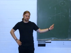
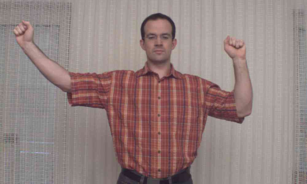
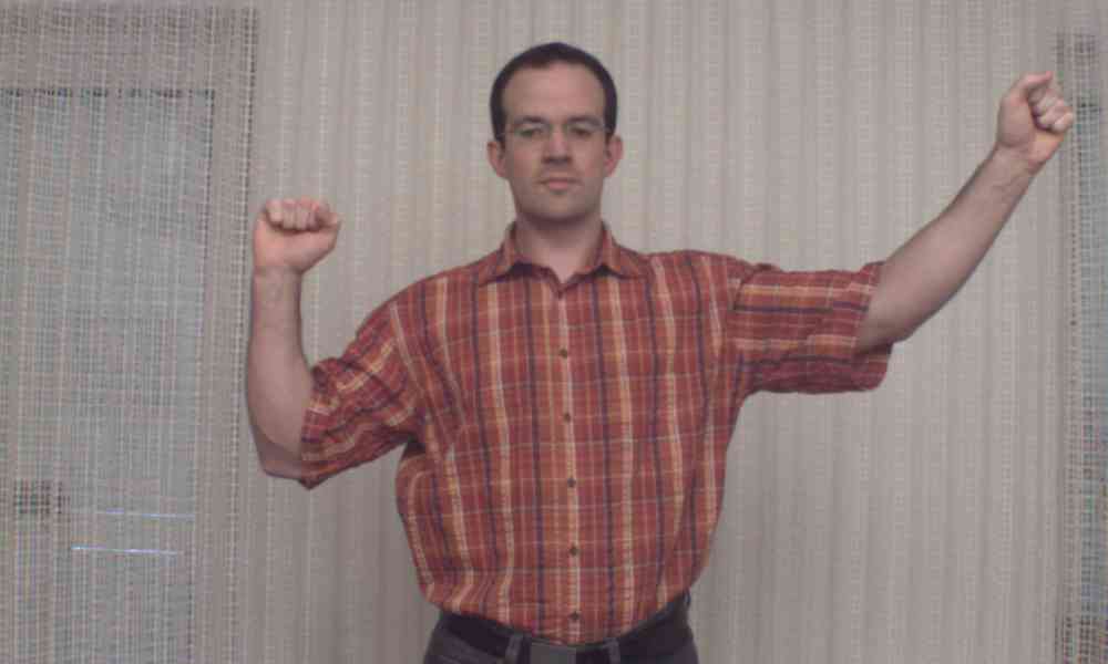
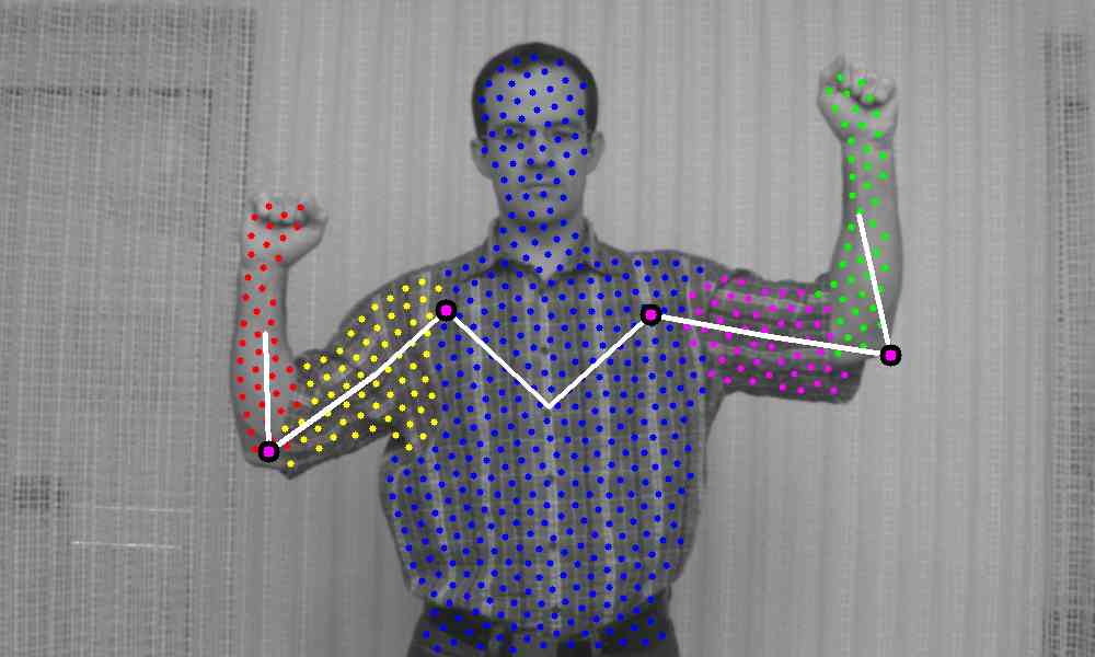
Based on these fundamental rules, fully autonomous extraction of sequence-specific HBMs from short input video streams of low visual complexity becomes viable (Fig. 1 b). Three exemplary frames from an input sequence are sketched in Fig. 2a through 2c.

III-A Acquiring limb patterns from video input

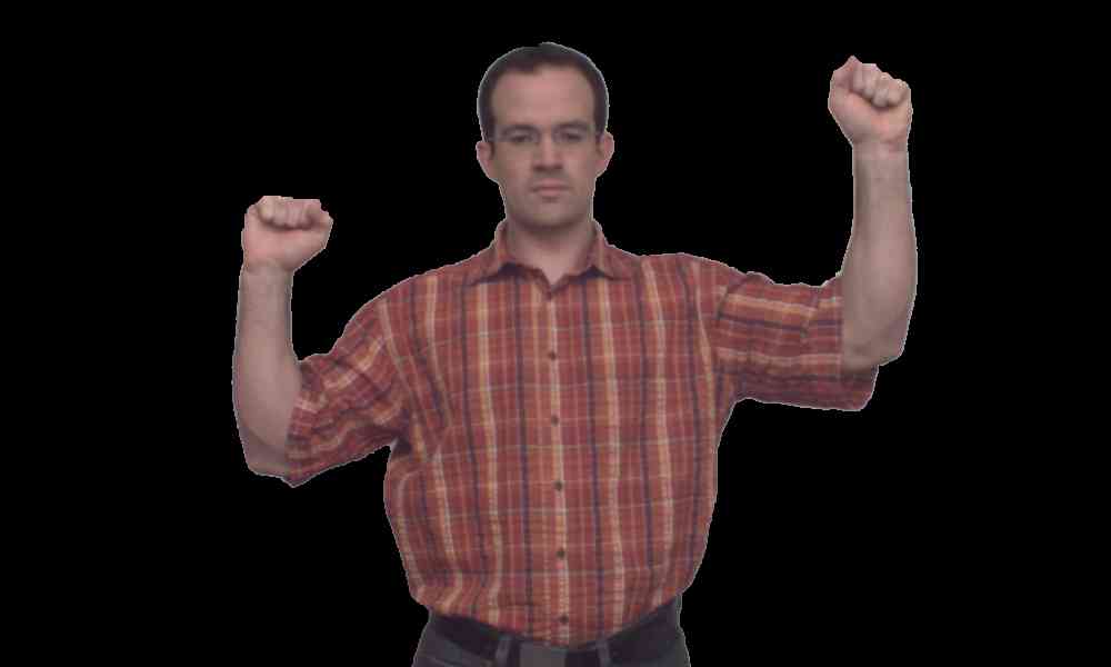
We begin by retrieving sequence-specific limb representations via coherent motion analysis (Fig. 1d): let $\overline{\text{DDI}}^{t}(\mathbf{x})$ represent the number of foreground active motion pixels (AMPs) in morphologically manipulated double difference images (DDI) (Kameda and Minoh, 1996) derived from a given input stream. From those, the reference frame $t^{*}$ is defined as the one with with maximal average DDI. The DDI-based foreground estimate in $I^{t^{*}}(\mathbf{x})$ yields a rough approximation of the foreground shape (the moving subject). A relatively sparse foreground map and a compact, dense background map are constructed using the graph cut segmentation of Boykov and Jolly (2001). Based on the maximum flow technique (Boykov and Kolmogorov, 2004), we employ the graph cut scheme of Mannan (2008) to perform precise foreground extraction in $I^{t^{*}}(\mathbf{x})$, (Fig. 2e). Remaining outliers in the resulting foreground proposal map $P^{t^{*}}_{\text{F}}(\mathbf{x})$ are eradicated via morphological closing (fig 1c).

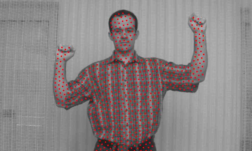
Next, the motion of the subject’s upper body is traced through all frames $t\neq t^{*}$ by applying Kanade-Lucas-Tomasi (Tomasi and Kanade, 1991) forward/backward tracking to $N_{\text{F}}$ features, which are distributed isotropically on the extracted foreground entity, (Fig. 2f). Inter-feature distance is automatically tuned using a test-and-repeat scheme to achieve constant $N_{\text{F}}$ for all input scenarios.

From the so generated feature trajectories initial estimates of body parts are retrieved. The trajectory for feature $i$ is the spatial time series $\mathbf{f}^{0}_{i},\ldots,\mathbf{f}^{(N_{\text{L}}-1)\Delta T}_{i}$, where $N_{\text{L}}$ is the number of frames and $\frac{1}{\Delta T}$ the frame rate. $\mathcal{V}$ is the complete set of $N_{\text{V}}$ trajectories $\mathbf{v}_{0},\ldots,\mathbf{v}_{N_{\text{V}}-1}$. The pairwise trajectory distances are expressed via (modified from (Krahnstoever, 2003))

$$d(\mathbf{v}_{i},\mathbf{v}_{j}) = \alpha\sum^{N_{\text{L}}-1}_{t=0}(\Delta_{ij}^{t}-\overline{\Delta}_{ij})^{2}$$ (1)

$$+ (1-\alpha)\sum^{N_{\text{L}}-2}_{t=0}{\left(1-\left\langle\mathbf{vel}_{i}^{t},\mathbf{vel}_{j}^{t}\right\rangle\right)}$$

with $\Delta_{ij}^{t}=\left\|\mathbf{f}_{i}^{t}-\mathbf{f}_{j}^{t}\right\|$, $\mathbf{vel}^{t}_{i}=\mathbf{f}_{i}^{t+1}-\mathbf{f}_{i}^{t}$, and $\overline{\Delta}_{ij}$ is the mean of $\Delta^{t}_{ij}$ over all frames. $\left\langle\cdot,\cdot\right\rangle$ represents the scalar product, $\alpha=0.01$.

Eq. (1) is plugged into a self-tuning (Zelnik-Manor and Perona, 2004) framework to extract perceptually consistent limb representations without manual intervention. We employ iterative normalized cut clustering to segment the trajectory dataset. Instead of $\text{NCut}(\mathcal{V}_{0},\mathcal{V}_{1})$ (Shi and Malik, 2000) that splits the trajectory set $\mathcal{V}$ in two child clusters we use

$$\text{NCut}^{\prime}(\mathcal{V}_{0},\mathcal{V}_{1})=\text{NCut}(\mathcal{V}_{0},\mathcal{V}_{1})e^{-\frac{\sigma_{\text{b}}^{2}-\alpha_{\text{b}}}{\beta_{\text{b}}}}\,,$$ (2)

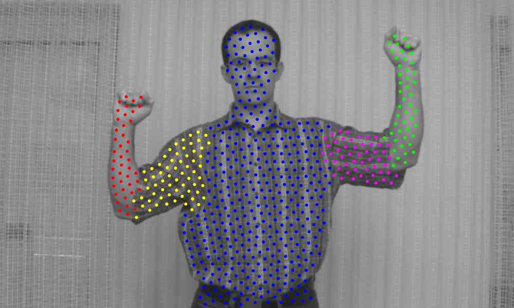
with empirically determined values of $\alpha_{\text{b}}=20.0$ and $\beta_{\text{b}}=200.0$. If this value exceeds $\tau_{\text{NC}}=0.35$, or if the number of features in any child cluster becomes $\leq 10$, splitting is stopped. With such a large threshold, the trajectory sets may become oversegmented; excess clusters are primarily caused by non-rigid cloth motion. Cloth-induced clusters generally arise from distortion of attire, and rarely show significant motion relative to the respective limbs. Clusters representing true body parts tend to move vividly and to rotate relative each other due to the rotatory connections enforced by the underlying kinematic skeleton (cf. (Walther, 2011)). As a consequence, all feature clusters with a relative rotation of less than $15^{\circ}$ and with a mutual barycenter shift of less than 10 pixels are merged, which reliably eliminates cloth-induced excess clusters. Prior to the merging stage, statistical outlier removal eliminates all features whose time course strays significantly from that of their host cluster. The number of clusters after merging is $N_{\text{G}}$, the clusters are identified by $\mathcal{G}_{i}$ and shown for the reference frame in Fig. 2g.

III-B Retrieving kinematic skeletons

Recent skeleton extraction approaches include (Yan and Pollefeys, 2008; Ross et al., 2010) – for the current work, the one by (Krahnstoever, 2003) is favored. There, skeleton extraction is applied to full limb templates, here we retrieve skeletons at an earlier stage directly from feature group data; the quality of the results is comparable to those of Krahnstoever (2003). We use a different distance-based joint plausibility criterion:

$$s^{k}_{ij}=\min\limits_{u}\left\|\mathbf{x}_{ij,\text{wrl}}^{0*}-\mathbf{f}^{0}_{u}\right\|,\ \mathbf{f}^{0}_{u}\in\mathcal{G}_{k},\ k\in\{i,j\}\,.$$ (3)

$\mathbf{x}_{ij,\text{wrl}}^{0*}$ is the world position at $t=0$ of a putative joint between feature groups $\mathcal{G}i$ and $\mathcal{G}j$. Eq. (3) causes alteration of Krahnstoever’s (2003) original values from $a_{s}^{+}=1$ and $a_{s}^{-}=10$ to $a_{s}^{+}=20$, $a_{s}^{-}=100$ in our implementation (see (Walther, 2011) for details). Fig. 2h demonstrates the performance of this scheme on the previously segmented input scenario (Fig. 2g).

III-C Generating limb templates

Although sufficient for skeleton extraction, the sparse body part patterns give only an approximation of true human limb shape and must be fleshed to compact limb templates. All pixels $\mathbf{x}:P^{t^{*}}_{\text{F}}(\mathbf{x})=1$ of $\mathbf{I}^{t^{*}}(\mathbf{x})$ (color frame) are assigned to limb template $i$ using

$$D_{k}(\mathbf{x}) =\min\limits_{\mathbf{f}^{t^{*}}_{j}\in\mathcal{G}_{k}}\left\|\mathbf{f}^{t^{*}}_{j}-\mathbf{x}\right\|$$

$$i_{\text{for pixel}\mathbf{x}} =\arg\min\limits_{i^{\prime}=0,\ldots,N_{\text{G}}-1}D_{i^{\prime}}(\mathbf{x})\,.$$ (4)

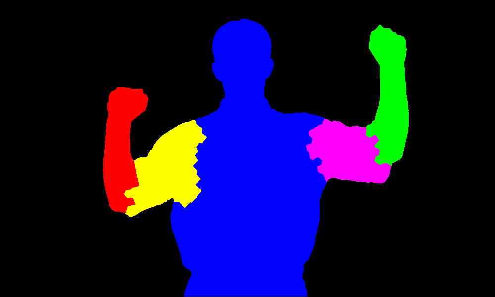
The resulting limb masks are exemplarily depicted in Fig. 2i, color templates for each body part $i$ can easily be learned by collecting information in areas of $\mathbf{I}^{t^{*}}(\mathbf{x})$ covered by the respective limb masks. Shape templates are constructed by scanning the outer perimeter of each mask, thus avoiding shape contributions from the foreground area. The learned body part templates do not take into account deformation behavior of human limbs, but in downstream processing, such deformation will be averaged out anyway.

III-D Pictorial structures for upper human body modeling

It remains to cast the extracted templates and kinematic constraints into a concise body pattern, which is represented by a pictorial structure model (Fischler and Elschlager, 1973; Felzenszwalb and Huttenlocher, 2000). Our upper-body PS representations (Fig. 1h) allow to unify appearance and kinematic constraints of the observed subject. Each model comprises a tree-like graph with vertices representing the appearance of the body parts found in the limb extraction stage. Each graph edge encodes the ‘bones’ (kinematic constraints) of the previously extracted skeleton. The PS is further augmented with an array of joint angles learned for each retrieved body joint incorporating sequence-specific limb orientation information.

A detailed discussion of pictorial structures and matching strategies is left to (Felzenszwalb and Huttenlocher, 2000, 2005; Walther, 2011). We adopt matching techniques proposed by Felzenszwalb and Huttenlocher (2000, 2005) with the following modifications: A ‘switched’ slope parameter $k_{\theta}$ (which is constant in (Felzenszwalb and Huttenlocher, 2000) allows for integration of joint angle limits: if a joint’s rotation angle is within limits, $k_{\theta}$ remains small, ensuring nearly unconstrained joint motion, otherwise $k_{\theta}$ is significantly increased to penalize posture estimates violating learned joint ranges. Additionally, kinematic flips (Sminchisescu and Triggs, 2003) are tolerated in PS matching, deviating from (Felzenszwalb and Huttenlocher, 2000): model limbs may flip around their principal axes to better accommodate complex body postures. Joint angles are automatically adopted during the flipping process, which is restricted to both forearms.

For registering the PS model the input color image $\mathbf{I}(\mathbf{x})$ is first converted to a binary line image using the EDISON algorithm (Christoudias et al., 2002). Using oriented chamfer distance (Shotton et al., 2008), thinned (thinning routines from (Eriksen, 2006) representations of the learned limb perimeters are matched to the EDISON-based line representation (see (Walther, 2011) for details of this procedure).

IV Meta model formulation

These PS models are highly scenario-specific and will be inadequate for posture estimation in novel situations. A model learned from a subject wearing a red short-sleeve shirt will likely fail to match another subject wearing a green long-sleeve shirt. Nevertheless, the sequence-specific PS models created above might well be consolidated to yield a more generic and powerful meta model (Walther and Würtz, 2010) $\mathbf{M}_{\text{meta}}$ that represents the upper human body on an abstract, conceptual level (Fig. 1m).

To that end, let $\mathcal{M}=[\mathbf{M}_{0},\ldots,\mathbf{M}_{N_{\text{M}}-1}]$ represent an array of body models extracted from $N_{\text{M}}$ sequences using the techniques proposed above. For each model $\mathbf{M}_{i}$ $\mathcal{S}_{i}=[\mathbf{s}_{i,0},\ldots,\mathbf{s}_{i,{N_{\text{G}}-1}}]$ is the array of smoothed and normalized shape templates. Smoothing is of Gaussian type (using a standard deviation of 5 pixels) and helps to cope with moderate cloth deformation, cf. (Walther, 2011). Subsequent normalization forces all values in the smoothed template into $[0,1]$. In addition, let $\mathcal{C}_{i}=[\mathbf{c}_{i,0},\ldots,\mathbf{c}_{i,{N_{\text{G}}-1}}]$ constitute the color templates retrieved for each limb of $\mathbf{M}_{i}$. Further, be $\mathcal{O}_{i,j}$ an array containing all observed orientations of $\mathbf{M}_{i}$’s $j$^th limb. Any model $i$ contains a constant number $N_{\text{J}}$ of joints, and comprises an array $\mathcal{W}_{i,k}$, which aggregates all joint angles observed for joint $k$.

$\mathbf{M}_{\text{meta}}$ also holds a shape accumulator array $\mathcal{S}_{\text{acc}}=[\mathbf{s}_{\text{acc},0},\ldots,\mathbf{s}_{\text{acc},N_{\text{G}}-1}]$ and a color accumulator array $\mathcal{C}_{\text{acc}}=[\mathbf{c}_{\text{acc},0},\ldots,\mathbf{c}_{\text{acc},N_{\text{G}}-1}]$ for each meta limb. The accumulators for meta limb $j$ are related to the meta model’s body part representations according to

$$\mathbf{s}_{\text{meta},j}=\frac{\mathbf{s}_{\text{acc},j}}{N_{\text{I}}},\ \mathbf{c}_{\text{meta},j}=\frac{\mathbf{c}_{\text{acc},j}}{N_{\text{I}}}\,.$$ (5)

$N_{\text{I}}$ indicates the number of sequence-specific models already integrated into $\mathbf{M}_{\text{meta}}$. There is also a joint position accumulator array, discussed in (Walther, 2011).

To initialize the meta model, let $\mathbf{M}_{\text{meta}}=\mathbf{M}_{0}$. Limb templates from $\mathbf{M}_{0}$ are copied into the accumulators of the meta model, $N_{\text{I}}$ is accordingly set to 1. In addition, topology and connectivity are cloned from $\mathbf{M}_{0}$, as well as joint limits and angular distributions.

IV-A Aligning the input models

Integrating information from each $\mathbf{M}_{i}$ ($i>0$) into the evolving meta model is a concept building task. The meta limb prototypes (i. e., the limb templates of $\mathbf{M}_{\text{meta}}$) are updated by sequentially adding information from all $\mathbf{M}_{i}$ ($i>0$) to $\mathbf{M}_{\text{meta}}$. To ease that process, the structure of each incoming model $\mathbf{M}_{i}$ is aligned to match the current meta model structure w. r. t. body part alignment, limb enumeration, and joint enumeration. To that end, $\mathbf{M}_{i}$ is instantiated to take on a typical posture by setting each of the model’s joints to the center angle halfway in between the links’ upper and lower limits. Directional statistics (Mardia and Jupp, 2000) are used to find these center angles. The designated root limb acts as an anchor in the instantiation process and is fixed to its mean orientation. Thinned limb shapes of the instantiated model are then projected to an artificial query image $I_{\text{a}}(\mathbf{x})$. Barycenter coordinates of each projected shape template $\mathbf{s}_{i,j}$ are stored in $\mathbf{b}_{i,j}$. The current $\mathbf{M}_{\text{meta}}$ is matched to $I_{\text{a}}(\mathbf{x})$, using the PS matching routines discussed in (Walther, 2011). After matching, barycenters $\mathbf{b}_{\text{meta},k}$ of the meta model should project near the $\mathbf{b}_{i,j}$ if only if meta limb $k$ corresponds to limb $j$ in $\mathbf{M}_{i}$. Then meta limb $k$ is defined to correspond to model limb

$$j=\arg\min\limits_{j^{\prime}}\left\|\mathbf{b}_{\text{meta},k}-\mathbf{b}_{i,j^{\prime}}\right\|$$ (6)

Knowing all limb correspondences, $\mathbf{M}_{i}$ can readily be manipulated to comply with the meta model’s current structure: limb and joint enumeration are unified by reindexing, using the retrieved correspondences. After reindexing, limb $j$ in model $i$ corresponds to meta limb $j$ and joint $k$ of $\mathbf{M}_{i}$ corresponds to meta joint $k$. With that, body-centric coordinate systems of all limbs in $\mathbf{M}_{i}$ are adjusted such that limb focusing in $\mathbf{M}_{i}$ and $\mathbf{M}_{\text{meta}}$ becomes identical; thorough bookkeeping is necessary to keep values in each $\mathcal{O}_{i,j}$ and each $\mathcal{W}_{i,k}$ consistent. After these preparations, $\mathbf{M}_{i}$ is aligned with the current meta model.

IV-B Learning meta shape prototypes

Formulating prototypical shapes (Fig. 1i) for a structure that deforms as vividly as a dressed human limb is not trivial, we rely on the approximate registration between each shape template $\mathbf{s}_{i,j}$ of $\mathbf{M}_{i}$ and the corresponding meta shape prototype $\mathbf{s}_{\text{meta},j}$. Based on that, a registration operator applies the 2D iterative closest point (ICP) method of Besl and McKay (1992), accelerated according to Rusinkiewicz and Levoy (2001), to compensate for the residual alignment failure between the shape representations. Following ICP registration, $\mathbf{s}_{i,j}$ and $\mathbf{s}_{\text{meta},j}$ are assumed to be aligned optimally in the sense of Besl and McKay (1992). The aligned $\mathbf{s}_{i,j}$ is eventually summed into $\mathbf{s}_{\text{acc},j}$; this summation for all $i>0$ yields a voting process (Lee and Grauman, 2009): shape pixels strongly voted for by constantly high accumulator values evolve into persistent outline modes, whereas areas not supported by given evidence fade out during aggregation. After adding $\mathbf{s}_{N_{\text{M}}-1,j}$, the weakest 25 percent of the collected votes are removed from the accumulator in order to memorize only reliable outline segments for each processed body part.

IV-C Acquiring meta color prototypes

Learning meta color prototypes (Fig. 1j) is more involved than shape prototype construction: assuming that color information from some sequence-specific model $\mathbf{M}_{i}$ shall be exploited to update the meta color prototypes, results from above matching/ICP registration can be carried forward to align color prototype $\mathbf{c}_{i,j}$ with the corresponding color accumulator $\mathbf{c}_{\text{acc},j}$. The aligned color representations are mapped to HSV color space and pixelwise color similarities are measured by HS-histogram-based windowed correlation. The V-component is dropped in order to increase robustness against illumination variation (Elgammal et al., 2009). A binary persistent color mask $M_{i,j}(\mathbf{x})$ is then defined such that pixels in $M_{i,j}(\mathbf{x})$ take on ‘1’ values if and only if the correlation result at image location $\mathbf{x}$ exceeds a threshold of 0.25. Guided by $M_{i,j}(\mathbf{x})$, information from $\mathbf{c}_{i,j}$ is used to update the meta model’s $j$^th color accumulator, according to

$$\mathbf{c}_{\text{acc},j}(\mathbf{x})=\begin{cases}\mathbf{c}_{\text{acc},j}(\mathbf{x})+\mathbf{c}_{i,j}(\mathbf{x})&\text{if }M_{i,j}(\mathbf{x})>0\\ \mathbf{0}&\text{otherwise}\end{cases}\,.$$ (7)

When applied to all $\mathbf{c}_{i>0,j}$, eq. 7 suppresses color information that varies significantly between sequences. Persistent colors are preserved as desired and yield, via eq. (5), the prototypes $\mathbf{c}_{\text{meta},j},j\in\{0,\ldots,N_{\text{G}-1}\}$. Any $\mathbf{c}_{\text{meta},j}$ is considered valid if it contains at least one nonzero pixel.

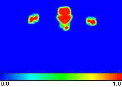
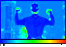
Now each $\mathbf{c}_{\text{meta},j}$ is augmented with an HS-histogram $\mathcal{H}_{\text{meta},j}$ that allows for histogram backprojection (Swain and Ballard, 1991). To populate $\mathcal{H}_{\text{meta},j}$, a complex sampling scheme is employed; see (Walther, 2011) for details. Backprojecting $\mathcal{H}_{\text{meta},j}$ to novel image content yields the backprojection map $C_{j}(\mathbf{x})$ for the corresponding body part. Windowed histogram backprojection is employed here in order to increase compactness of the generated maps. For posture estimation the backprojection maps are thresholded at 10% of their peak and blurred by a Gaussian with a standard deviation of 5.0 pixels. Follow-up normalization forces $C_{j}(\mathbf{x})$ into $[0,1]$, all entries in backprojection maps corresponding to meta limbs without valid color prototype are set to 1.0. Fig. 7b (additional material) exemplarily shows $C_{\text{torso}}(\mathbf{x})$ resulting from backprojection of $\mathcal{H}_{\text{meta},\text{torso}}$ to the query image in Fig. 7a (additional material). Based on $C_{j}(\mathbf{x})$, the color cue map $C_{\theta_{j},s_{j}}(\mathbf{x})$ for meta limb $j$ with orientation $\theta_{j}$ and scale $s_{j}$ is readily defined: let $\mathbf{c}^{\prime}_{\text{meta},j}$ be a binarized representation of $\mathbf{c}_{\text{meta},j}$, with $\mathbf{c}^{\prime}_{\text{meta},j}(\mathbf{x})=1$ if and only if $\left\|\mathbf{c}_{\text{meta},j}(\mathbf{x})\right\|>0$. Then be $\mathbf{c}^{\prime}_{\text{meta},\theta_{j},s_{j}}$ an instance of $\mathbf{c}^{\prime}_{\text{meta},j}$, oriented and scaled as to match meta limb $j$’s desired state. With that

$$C_{\theta_{j},s_{j}}(\mathbf{x})=\frac{C_{j}(\mathbf{x})*\mathbf{c}^{\prime}_{\text{meta},\theta_{j},s_{j}}}{\sum\mathbf{c}^{\prime}_{\text{meta},\theta_{j},s_{j}}}\,,$$ (8)

where ‘$*$’ is convolution and the sum aggregates all nonzero pixels in $\mathbf{c}^{\prime}_{\text{meta},\theta_{j},s_{j}}$.

IV-D Gabor prototype generation

Besides shape and color information persistent texture can be learned autonomously from given input data (Fig. 1k). To that end, we employ Gabor wavelets as tuneable, localized frequency filters in the construction of Gabor grid graphs for each meta limb $i$. Graph nodes correspond to mean Gabor magnitude jets (cf. (Lades et al., 1993)) $\mathbf{J}_{i,j},\ j=0,\ldots,N_{\text{Q},i}-1$ learned from the input streams. The jet learning scheme uses the same batch process as employed for color prototyping (cf. (Walther, 2011)). Given the mean jets, batch learning is restarted to calculate each jet $j$’s covariance matrix, whose largest eigenvalue $\lambda^{*}_{i,j}$ provides a convenient measure of the node’s reliability $\eta_{i,j}=1/\sqrt{\lambda^{*}_{i,j}}$. In our approach, two normalized complex jets $\mathbf{J}_{\text{A}}$ and $\mathbf{J}_{\text{B}}$ are compared by inspecting their absolute parts only (Lades et al., 1993).

$$S_{\text{Abs}}\left(\mathbf{J}_{\text{A}},\mathbf{J}_{\text{B}}\right)=\sum_{j}a_{\text{A},j}a_{\text{B},j}$$ (9)

Being exclusively interested in persistent texture, all nodes with reliabilities $\eta_{i,j}<5.0$ are pruned. The largest connected subgraph $G^{*}_{\text{G},i}$ that survives this procedure makes up a valid Gabor prototype for meta limb $i$ if and only if its node count $N^{*}_{\text{Q},i}$ exceeds 50; this large threshold restricts prototype learning to meaningful Gabor patches. Henceforth, define the nodes of prototype graph $i$ to be $\mathbf{g}_{i,j},\ j=0,\ldots,N^{*}_{\text{Q},i}-1$. In our experiments, a valid Gabor prototype evolved exclusively on the head region; potential Gabor patterns for all other limbs were depleted of nodes by pruning and became invalid. Note that our system learns to treat the head and the thorax region of an observed subject as a single torso entity, because the training data did not include movement between the two. Thus, the evolved Gabor prototype can be seen as a generic texture-based torso detector that optimally responds to human torsi in upright position.

A Gabor jet representation $\mathcal{G}_{I}\left(\mathbf{x}\right)$ of query image $I(\mathbf{x})$ yields a Gabor cue map for meta limb $i$ in orientation $\theta_{i}$ and with scale $s_{i}$:

$$G_{\theta_{i},s_{i}}(\mathbf{x}) = 1-\frac{1}{N^{*}_{\text{Q},i}}\sum\limits_{\mathbf{g}_{i,j}\in G^{*}_{\text{G},i}}S_{\text{Abs}}\left(\mathbf{J}_{i,j},\mathbf{J}_{I}\right),$$

$$\mathbf{J}_{I} = \mathcal{G}_{I}\left(\mathbf{x}+\mathcal{P}_{\theta_{i},s_{i}}\left(\mathbf{g}_{i,j}\right)\right)\,,$$ (10)

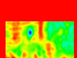
where $\mathcal{P}_{\theta_{i},s_{i}}\left(\cdot\right)$ projects nodes of $G^{*}_{\text{G},i}$ into $I(\mathbf{x})$. Fig. 8 (additional material) demonstrates application of the learned torso detector (in upright position and with scale 1.0) to the image in Fig. 8a: the observed torso barycenters correspond to pronounced minima in the Gabor cue map depicted in Fig. 8b.

IV-E Limb pre-detection

Rotation of any meta limb $i$ with valid Gabor prototype $G^{*}_{\text{G},i}$ can safely be assumed negligible (Walther, 2011). This allows to condense the orientation dimension of the meta limb’s state space to a single, typical value $\theta_{\text{typ},i}$ which corresponds to the mean of all body part orientations observed during model learning. Accordingly, we define the color-augmented Gabor detection map for meta limb $i$, presuming that a valid $G^{*}_{\text{G},i}$ exists

$$\overline{G}_{\theta_{\text{typ},i},s_{i}}(\mathbf{x})=\begin{cases}\frac{1}{2}G(\mathbf{x})&\text{if }G(\mathbf{x})<\frac{\widehat{G}}{2}\text{ and }C(\mathbf{x})>\frac{\widehat{C}}{2}\\ G(\mathbf{x})&\text{otherwise}\,,\end{cases}$$ (11)

where $G(\mathbf{x})$ is a shortcut for $G_{\theta_{\text{typ},i},s_{i}}(\mathbf{x})$, $C(\mathbf{x})$ stands for $C_{\theta_{\text{typ},i},s_{i}}(\mathbf{x})$; $\widehat{G}$ is the peak value of $G_{\theta_{\text{typ},i},s_{i}}(\mathbf{x})$ and $\widehat{C}$ represents the largest value of $C_{\theta_{\text{typ},i},s_{i}}(\mathbf{x})$. Combining the two ‘weak’ cues in eq. (11), the system successfully eliminates wrong detection optima in all performed experiments. With that,

$$s_{\text{pre},i}=\arg\min\limits_{s}\left(\min\limits_{\mathbf{x}}\overline{G}_{\theta_{\text{typ},i},s}(\mathbf{x})\right)$$ (12)

yields the most probable scale estimate for meta limb $i$ given texture and color evidence in input image $\mathbf{I}(\mathbf{x})$. Minimization in eq. (12) is performed with 30 discrete scales between 0.7 and 1.0. Going beyond scale, let

$$\mathbf{x}_{\text{pre},i}=\arg\min\limits_{\mathbf{x}}\overline{G}_{\theta_{\text{typ},i},s_{\text{pre},i}}(\mathbf{x})$$ (13)

and eventually assume meta limb $i$ to be pre-detected in location $\mathbf{l}_{\text{pre},i}=\left(\mathbf{x}_{\text{pre},i},\theta_{\text{typ},i},s_{\text{pre},i}\right)$. In the following experiments, positional search space for any pre-detectable meta limb $i$ is restricted to $\pm 10$ pixels around $\mathbf{x}_{\text{pre},i}$. Such body part anchoring acts, via given articulation constraints, on the complete meta model and allows to circumnavigate false local posture optima induced by background clutter. Thus, limb anchoring renders the final posture estimate more robust. Higher processing speed can be expected as a positive side effect of the anchoring procedure, as fewer state space locations have to be probed in the model matching cycle.

IV-F Enforcing color constancy

Scenarios with unrestricted illumination conditions require chromatic adaptation (Finlayson and Süsstrunk, 2000) like human perception (Hsu et al., 2008) to achieve approximate color constancy (Fig. 1l). This relies on persistently colored parts of the body to act as intrinsic color reference for autonomous chromatic adaptation, similar to (Montojo, 2009): first, input image $\mathbf{I}(\mathbf{x})$ is transformed to Lab opponent color space(Margulis, 2006; Montojo, 2009), yielding $\mathbf{I}_{\text{Lab}}(\mathbf{x})$. Lab space allows to remove unwanted color deviations by balancing the each pixel’s chromaticity coordinates until the cast vanishes while leaving luminance values largely unaltered. A shift vector of length $R_{i}\in\{0,2,4,8,16,32\}$ and direction $\gamma_{i}\in\{v_{i}\frac{2\pi}{8}:v_{i}=0,\ldots,7\}$ is added to the (a,b)-components of each pixel in $\mathbf{I}_{\text{Lab}}(\mathbf{x})$ and results in a color-shifted Lab input image $\mathbf{I}_{\text{Lab},R_{i},\gamma_{i}}(\mathbf{x})$. Conversion of $\mathbf{I}_{\text{Lab},R_{i},\gamma_{i}}(\mathbf{x})$ to HSV yields $\mathbf{I}_{\text{HSV},R_{i},\gamma_{i}}(\mathbf{x})$. A windowed backprojection (window size: 7x7 pixels) of $\mathcal{H}_{\text{meta},i}$ onto $\mathbf{I}_{\text{HSV},R_{i},\gamma_{i}}(\mathbf{x})$ gives the color similarity map $U_{R_{i},\gamma_{i}}(\mathbf{x})$, whose values are normalized to $[0;1]$.

Assuming existence of a valid Gabor prototype (and thus a valid $\mathbf{l}_{\text{pre},i}$) for meta limb $i$, the binary $\mathbf{c}^{\prime}_{\text{meta},i}$ are projected into the image plane (according to the parameters in $\mathbf{l}_{\text{pre},i}$); morphological opening follows to get rid of noise in the induced projection map $\mathbf{c}^{\prime}_{\text{meta},\mathbf{l}_{\text{pre},i}}$. From that we define the color similarity measure

$$C_{R_{i},\gamma_{i}}=\frac{\sum\limits_{\mathbf{x}:h(\mathbf{x})=1}U_{R_{i},\gamma_{i}}(\mathbf{x})}{\sum\mathbf{c}^{\prime}_{\text{meta},\mathbf{l}_{\text{pre},i}}}\,,$$ (14)

where $h(\mathbf{x})=\mathbf{c}^{\prime}_{\text{meta},\mathbf{l}_{\text{pre},i}}(\mathbf{x})$. Additionally, approximate a probability distribution

$$p_{R_{i},\gamma_{i}}(\mathbf{x})=\frac{U_{R_{i},\gamma_{i}}(\mathbf{x})}{\sum{U_{R_{i},\gamma_{i}}}}$$ (15)

with $\sum{U_{R_{i},\gamma_{i}}}$ being the sum of all entries in the color similarity map. This allows to set up the entropy of the color similarity map, according to

$$S_{R_{i},\gamma_{i}}=-\sum\limits_{\mathbf{x}\in\mathcal{X}}p_{R_{i},\gamma_{i}}(\mathbf{x})\ln(p_{R_{i},\gamma_{i}}(\mathbf{x}))\,.$$ (16)

$S_{R_{i},\gamma_{i}}$ grows large if the color distribution in $U_{R_{i},\gamma_{i}}(\mathbf{x})$ becomes diffuse, well-defined clusters bring the entropy down (Fig. 9, additional material). As persistent color patches stored in the meta limbs generally constitute coherent, compact structures, their footprints in $U_{R_{i},\gamma_{i}}(\mathbf{x})$ should (in the case of correctly chosen hyperparameters $R_{i},\gamma_{i}$) become blob-like; thus, color distributions with lower entropy are preferable. Optimal hyperparameters $(R^{*}_{i},\gamma^{*}_{i})$ are found according to

$$(R^{*}_{i},\gamma^{*}_{i})=\arg\max\limits_{R_{i},\gamma_{i}}\frac{C_{R_{i},\gamma_{i}}}{S_{R_{i},\gamma_{i}}}\,.$$ (17)

The corresponding Lab space shift vector that causes image colors (after conversion to RGB) to near persistent colors of meta limb $i$ to the utmost possible extent (w. r. t. color similarity and entropy) is defined as $\mathbf{s}^{*}_{i}=\mathbf{s}_{R_{i}^{*},\gamma_{i}^{*}}$. Fig. 11 (additional material) shows the efficiency of the chromatic adaptation routines employed here: the depicted backprojection maps for the torso’s histogram $\mathcal{H}_{\text{meta},\text{torso}}$ show significant improvement due to automatic color correction.

IV-G Augmenting the matching cost function

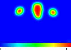
Given chromatically corrected input material, color information can be used to enhance the PS model matching procedure so far based on pure shape information. We define a negative stimulus map $N_{i}(\mathbf{x})$ that encodes a standard distance transformation on a morphologically opened, inverted instance of $\mathbf{c}^{\prime}_{\text{meta},\mathbf{l}_{\text{pre},i}}$. Subsequent normalization forces elements of $N_{i}(\mathbf{x})$ to lie in [0;1]. The complementary positive stimulus map is defined by $P_{i}(\mathbf{x})=1-N_{i}(\mathbf{x})$. The negative stimulus map is truncated at 0.3 to limit its influence on distant image structures. With that, a range of spatially biased backprojection maps for all meta limbs is initialized as $\overline{C}_{i}(\mathbf{x})=C_{i}(\mathbf{x})$, with $i=0,\ldots,N_{\text{G}}-1$. For any pre-detectable meta limb $i$, these maps are updated according to

$$\overline{C}_{j}(\mathbf{x}) = \begin{cases}\overline{C}_{j}(\mathbf{x})\cdot P_{j}(\mathbf{x})&\text{if }j=i\\ \overline{C}_{j}(\mathbf{x})\cdot N_{j}(\mathbf{x})&\text{if }j\neq i\end{cases}\,,$$ (18)

$$\overline{C}_{\theta_{i},s_{i}}(\mathbf{x}) = \frac{\overline{C}_{i}(\mathbf{x})*\mathbf{c}^{\prime}_{\text{meta},\theta_{i},s_{i}}}{\sum\mathbf{c}^{\prime}_{\text{meta},\theta_{i},s_{i}}}$$ (19)

These modified color cue maps give rise to a color-augmented matching cost function (see (Walther, 2011) for details)

$$m_{i}(\mathbf{l}_{i},\mathbf{I}(\mathbf{x}))=-\log\big{(}\big{.} \left[1-S_{\theta_{i},s_{i}}(\mathbf{x})\right]\cdot$$

$$\left.\left(0.65\cdot\overline{C}_{\theta_{i},s_{i}}(\mathbf{x})+0.35\right)\right)\,,$$ (20)

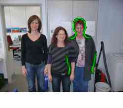
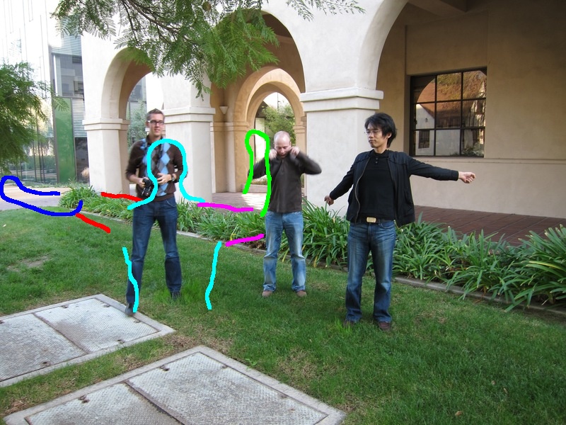
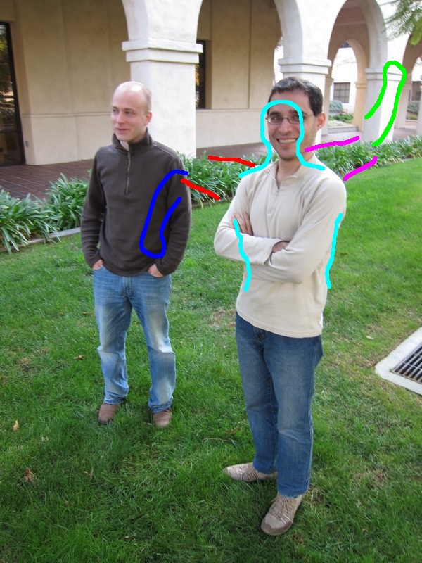
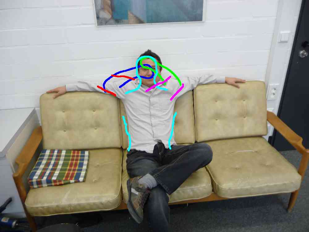
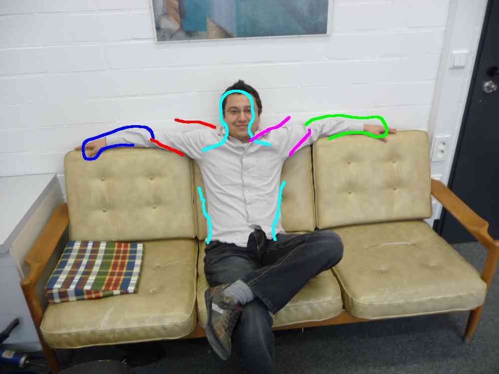
where scaling and offsetting prevent color from dominating shape information. As shown in Fig. 3, this can disambiguate complex double-counting (Ferrari et al., 2008) situations.

Benchmark	Permutation		Redundancy
image	$\mu_{\text{P},b}$	$\sigma_{\text{P},b}$	$\mu_{\text{R},b}$	$\sigma_{\text{R},b}$
A	9.8	0.92	9.3	0.3
B	9.1	3.8	6.6	0.5
C	8.8	1.8	8.9	0.5
D	11.2	1.4	10.8	0.4
E	9.5	2.3	9.5	0.3
F	7.1	1.4	6.5	0.5

TABLE I: Mean and standard deviation of matching results when permuting meta model assembly order (cols. 2, 3) and influence of redundant information (cols. 4, 5) on selected images (col. 1)

(a) Without stimulus maps

(b) Stimulus maps applied

Figure 3: Without stimulus maps, double-counting (Ferrari et al., 2008) can yield wrong posture estimates (s. Fig. 3a). Activating the stimulus maps (s. Fig. 3b) corrects this issue and yields perceptually valid results.

V Experimental evaluation

To test the posture inference (Fig. 1q) capabilities of the proposed meta model ‘in the wild’, we have recorded the INIPURE (Institut für NeuroInformatik – PostURe Estimation) database. This image set contains 63 upper body shots of adult subjects of different genders and age groups. Inter-subject variance in physique and worn attire is significant; a subject’s body pose may be severely foreshortened, background clutter and scene illumination are relatively unconstrained. For evaluation of matching, all images in the database have been manually annotated with ground-truth 2D posture information. All images (together with the system performance) are shown in figures 10 through 12. Raw images for comparison with other systems are available from the authors on request. This allows to compare our system’s matching performance with human intuition: let $\text{DT}_{b,i}(\mathbf{x})$ be a distance transformation map that stores the minimum Euclidean distance of any pixel in an INIPURE benchmark image $b$ (henceforth represented by $\mathbf{I}_{b}(\mathbf{x})$) to body part $i$’s manually labeled perimeter. Further, be $\mathbf{s}^{*}_{u,i}$ a binarized and thinned representation of meta model $u$’s $i$’th shape template, projected to $\mathbf{I}_{b}(\mathbf{x})$ according to our system’s optimal posture estimate. Nonzero pixels $\mathbf{h}_{u,i}\in\mathbf{s}^{*}_{u,i}$ shall be provided in $\mathbf{I}_{b}(\mathbf{x})$’s coordinate system. With that, the untruncated chamfer distance between $\mathbf{s}^{*}_{u,i}$ and the annotated perimeter of body part $i$ in benchmark image $b$ becomes (Shotton et al., 2008)

$$d_{u,i,b}=\frac{1}{\sum{\mathbf{s}^{*}_{u,i}}}\sum_{\mathbf{h}_{u,i}\in\mathbf{s}^{*}_{u,i}}\text{DT}_{b,i}\left(\mathbf{h}_{u,i}\right)\,,$$ (21)

where $\sum{\mathbf{s}^{*}_{u,i}}$ is the total number of nonzero pixels in $\mathbf{s}^{*}_{u,i}$. Eq. (21) allows to set up the limb-averaged model registration error $E_{u,b}$ as the average of all $N_{\text{G}}$ $d_{u,i,b}$.

V-A Reviewing the meta model

Based on $E_{u,b}$, the quality and robustness of our meta model can be assessed: in real-world settings, the succession of sequence-specific body models integrated into the meta model can hardly be controlled. Consequentially, the meta model’s matching performance has to be invariant against changes in model integration order. To check for such invariance, basic permutation tests suffice: a permutation table with $N_{\text{T}}=50$ rows and $N_{\text{M}}$ columns is set up with each row $r$ containing a random permutation of all $N_{\text{M}}$ body model indices. Processing the table row by row, sequence-specific body models are aggregated according to the row entries, forming interim meta models $\mathbf{M}_{\text{meta}_{r}}$. These models are then matched to 6 benchmark images selected from the INPURE database. To indicate good matching performance, both mean registration error $\mu_{\text{P},b}$ and standard deviation $\sigma_{\text{P},b}$ should stay as low as possible for all benchmark images; in particular, small standard deviations allow to deduce that model integration order does not significantly impact quality of posture inference. Cols. 2 and 3 of table I shows that this requirement is fulfilled, even for complex outdoor scenarios with severely cluttered background.

A follow-up benchmark test aims at assessing the system’s invariance against redundant information: given that the meta model assembly routines operate properly and extract all accessible information from the sequence-specific models, adding identical models multiple times should not significantly alter matching performance. Probing this hypothesis is straightforward: as model integration order was experimentally shown to be meaningless, a fixed, canonical sequence of input models is selected first.

Active switches	$\mu_{\mathcal{C}}$ (pixel)	$\sigma_{\mathcal{C}}$ (pixel)
$\tilde{S}$	171	113
$\tilde{S},\tilde{G}$	62	71
$\tilde{S},\tilde{G},\tilde{R}$	27	19
$\tilde{S},\tilde{G},\tilde{R},\tilde{C}$	23	19
$\tilde{S},\tilde{G},\tilde{R},\tilde{C},\tilde{M}$	14	10
$\tilde{S},\tilde{G},\tilde{R},\tilde{C},\tilde{M},\tilde{A}$	11	3

TABLE II: Mean and standard deviation of matching quality for different chosen cues.

Meta models $\mathbf{M}_{\text{meta}_{m}}$ are then learned by integrating the canonical model sequence $m$ times, where $m\in[0;N_{\text{C}}-1]$, with $N_{\text{C}}=10$. Posture estimation using each $\mathbf{M}_{\text{meta}_{m}}$ is performed on the above benchmark images; mean registration error and standard deviation are evaluated, and cols. 4 and 5 of table I shows that posture estimation results remain precise (small $\mu_{\text{R},b}$’s) and stable (small $\sigma_{\text{R},b}$’s), regardless of artificially enforced data redundancy.

(a)

(b)

(c)

Figure 4: Some results for the Perona challenge (Perona, 2012), see additional material for all of them.

V-B Hyperparameter settings

As both metamodel construction and matching are necessarily based on a combination of several methods from the literature, the number of hyperparameters from all these methods adds up, amounting to some 20 thresholds, template sizes, and other hyperparameters in this work. Fortunately, these are not independent but can be adjusted sequentially. Working on the given training set, the hyperparameters for background suppression, tracking and trajectory clustering were adjusted one after the other to get reasonable behavior. None of them are critical, no systematic optimization has been applied. The same goes for the hyperparameters of shape, color and Gabor cues as well as the combination parameters, which have been chosen using a subset of 6 images from the INIPURE dataset. These have been applied to the full dataset. The Perona dataset has been evaluated without any hyperparameter change. Of course, several hyperparameters imply assumptions about ranges of scale, image resolution, etc., which might need to be adjusted for new training data.

V-C Experiments on real-world footage

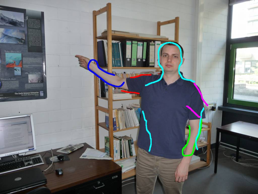
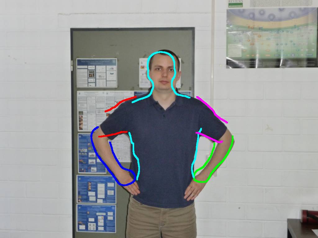
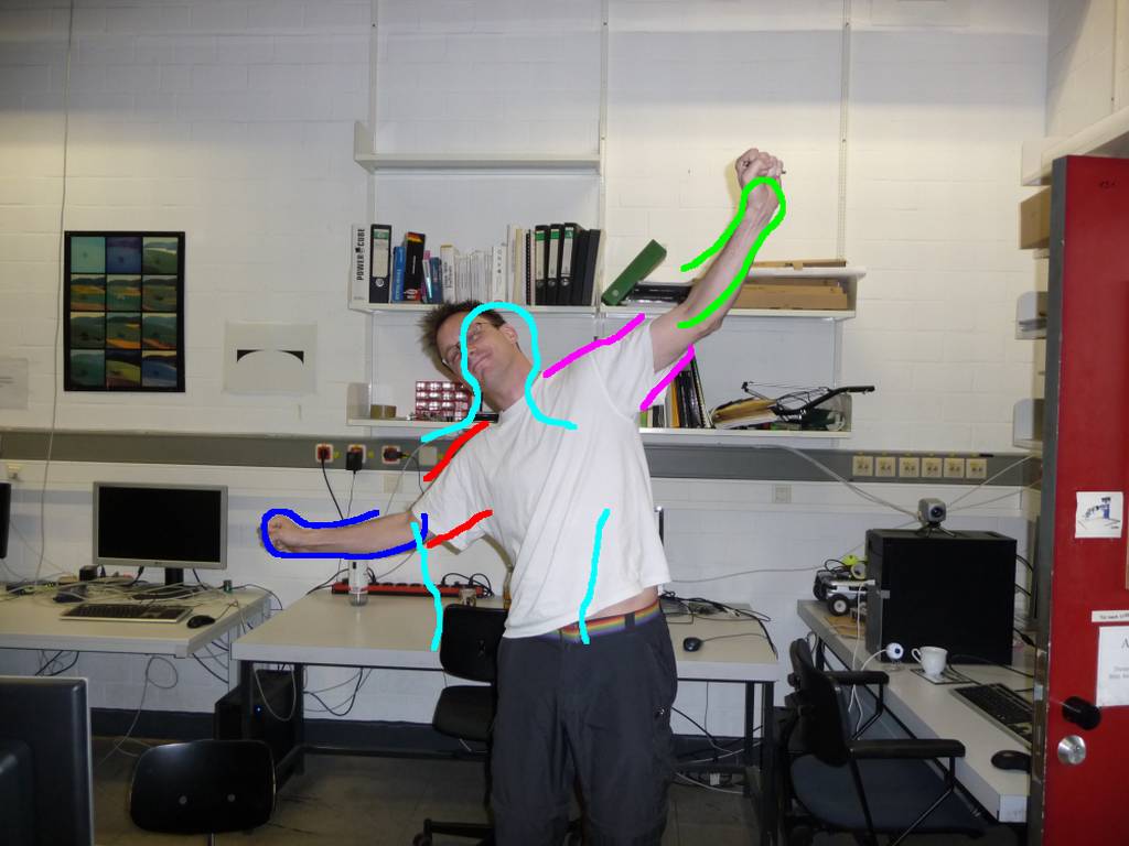
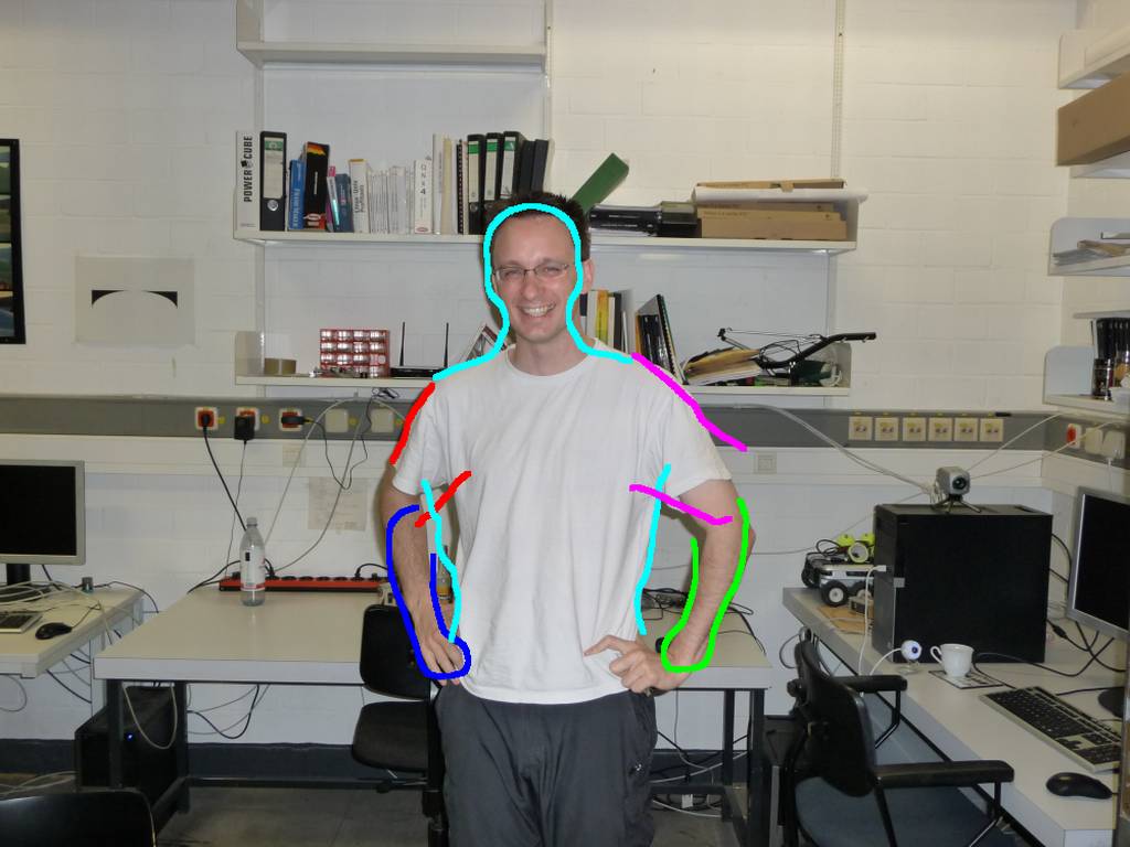
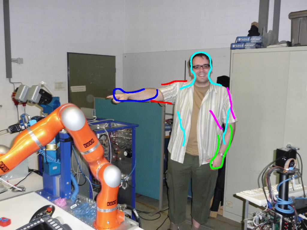
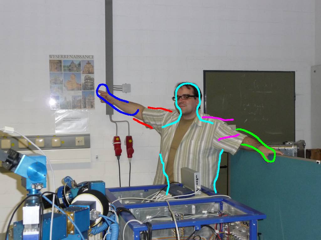
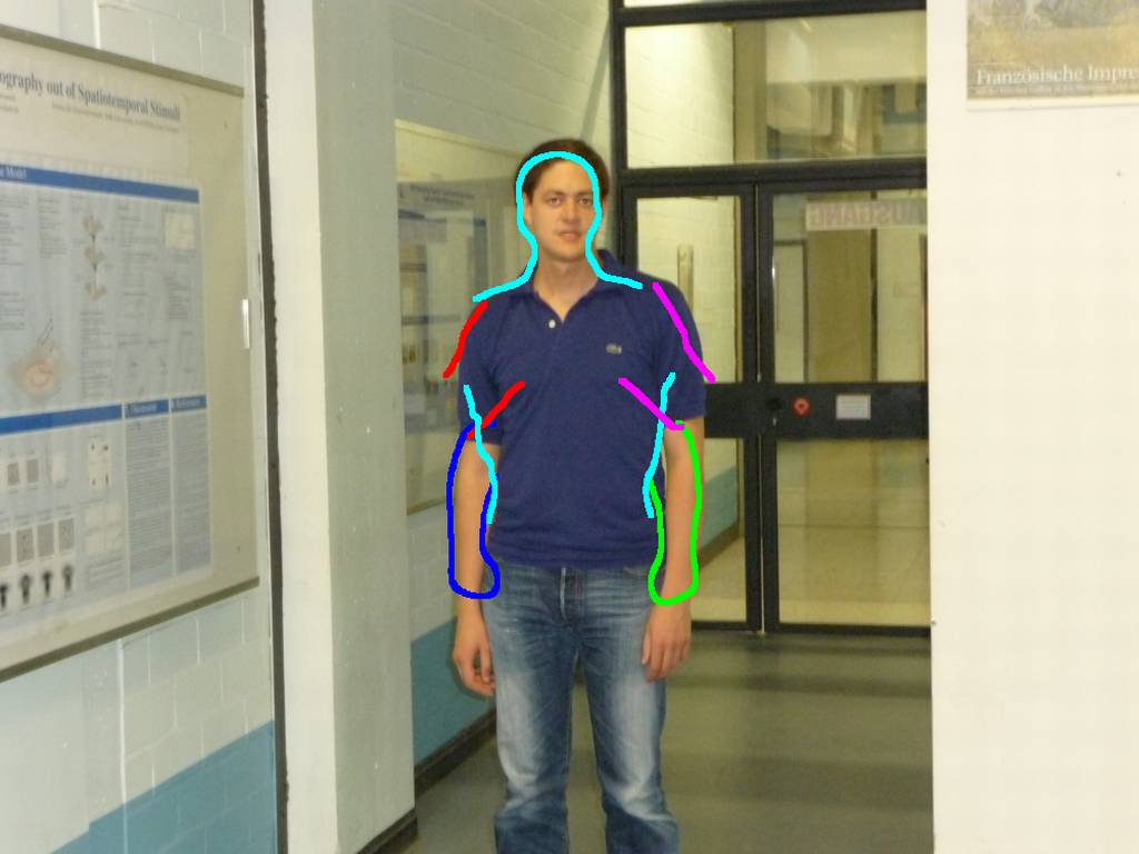
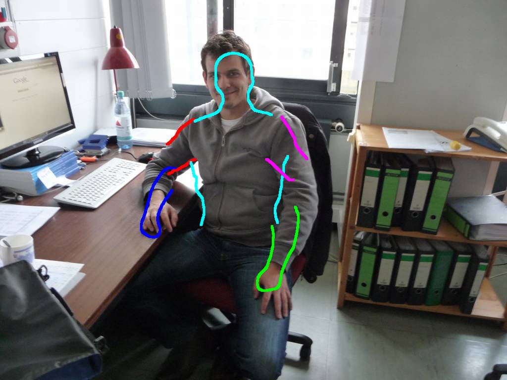
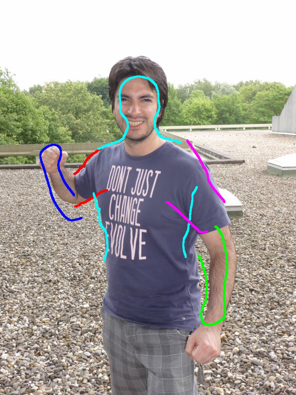
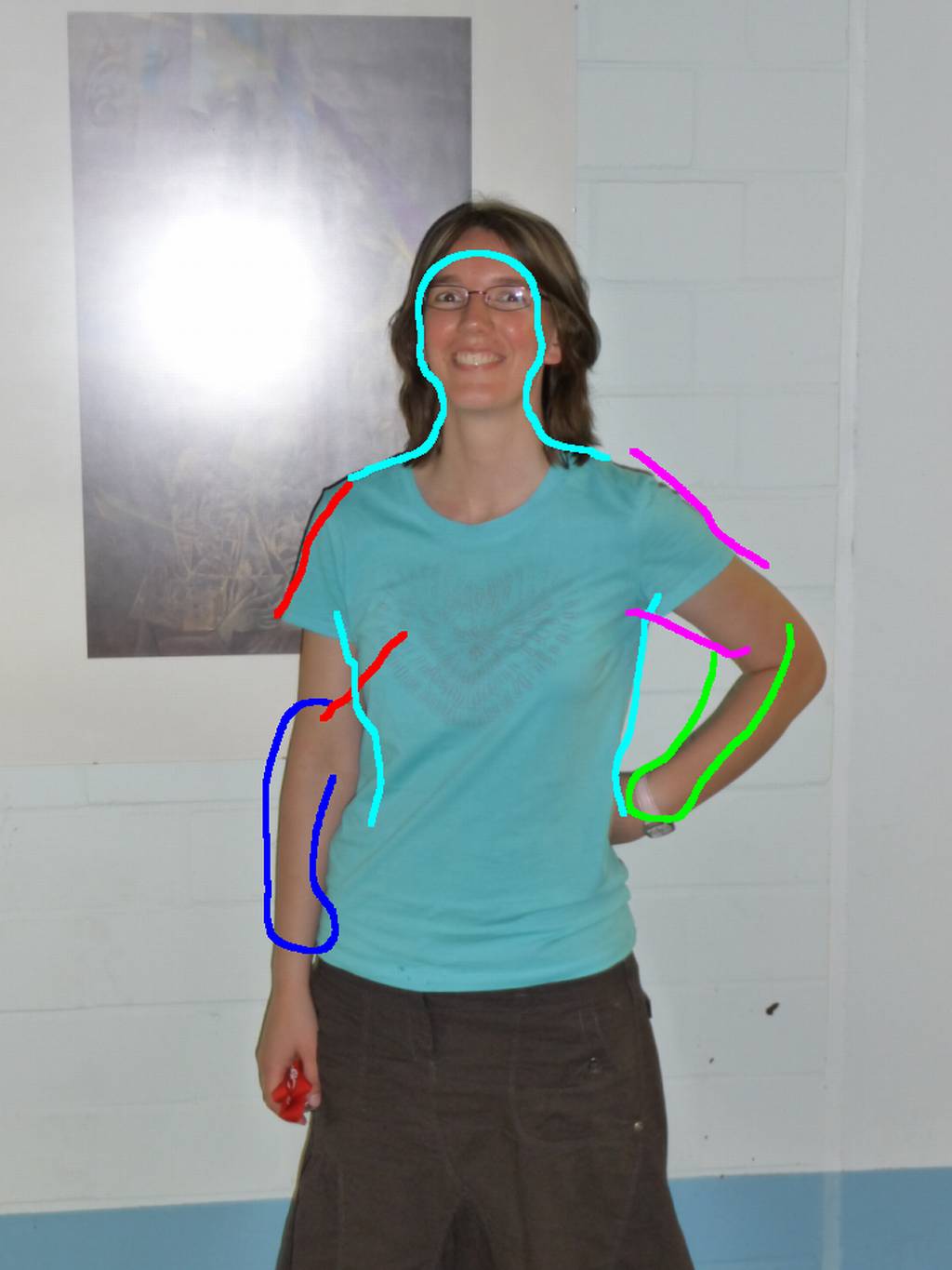
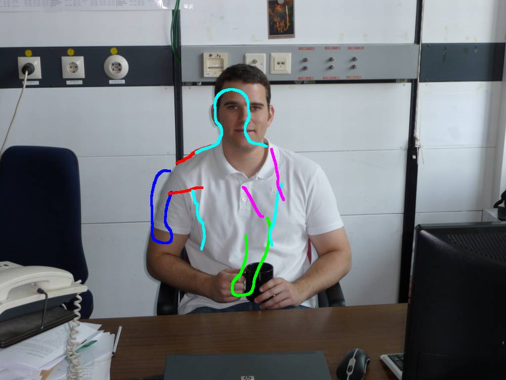
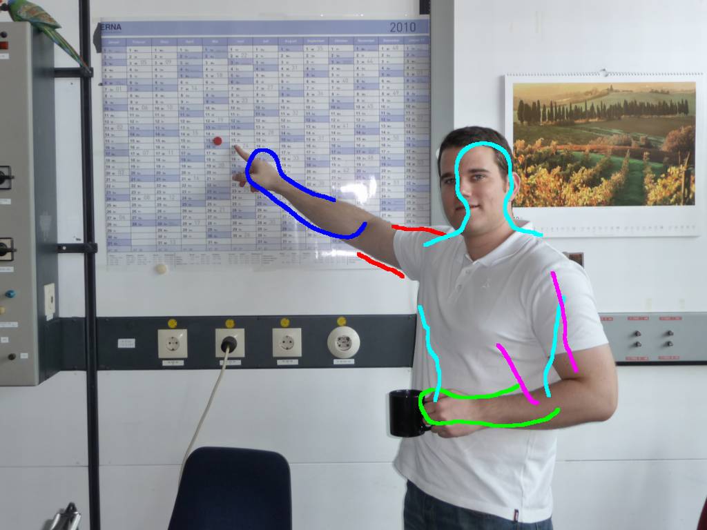
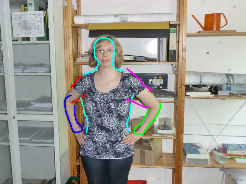
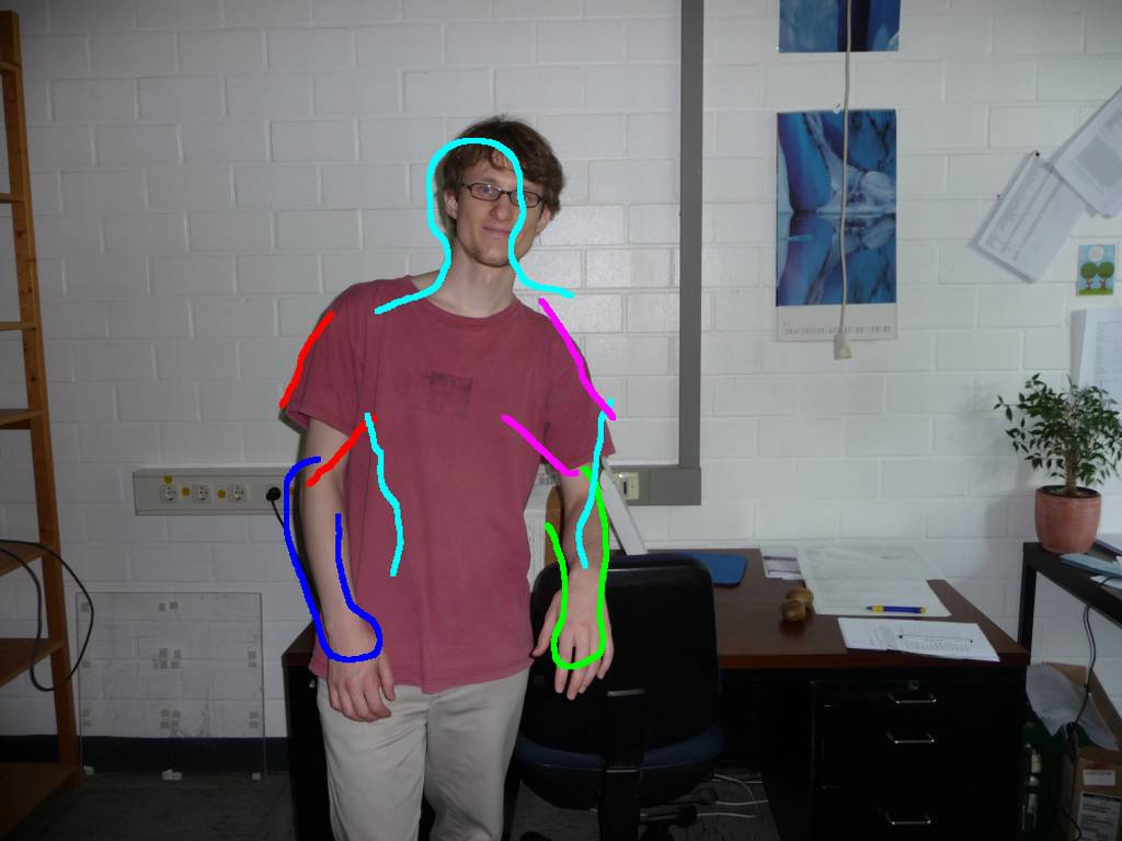
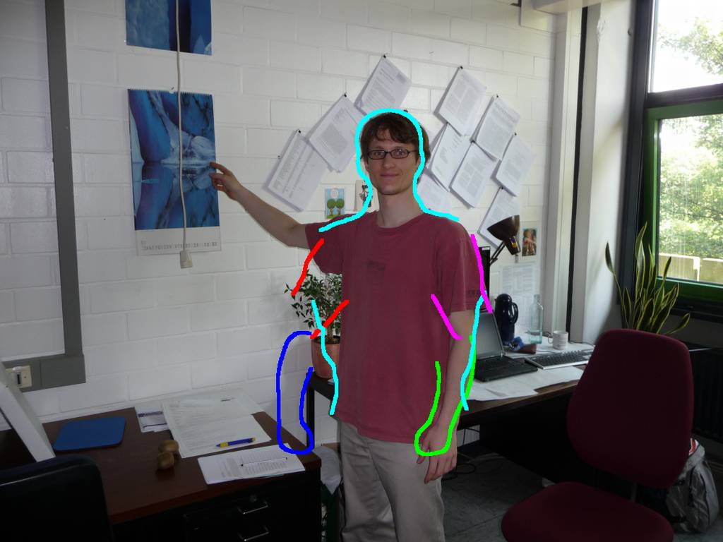
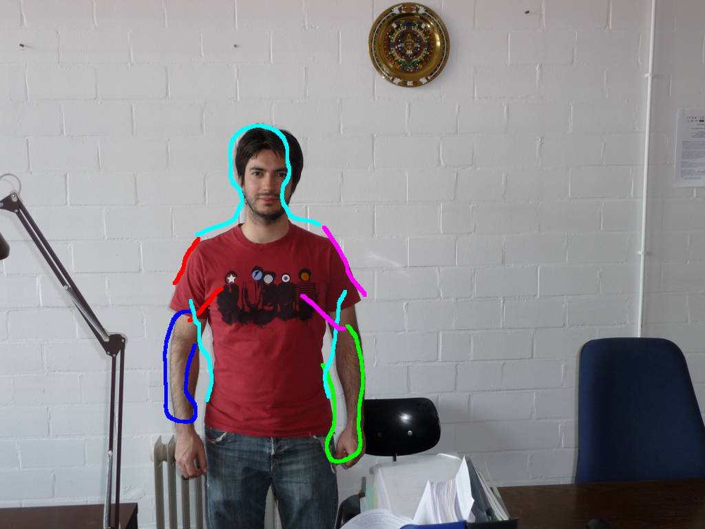
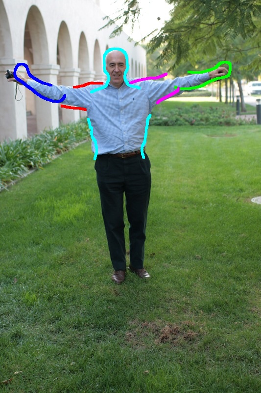
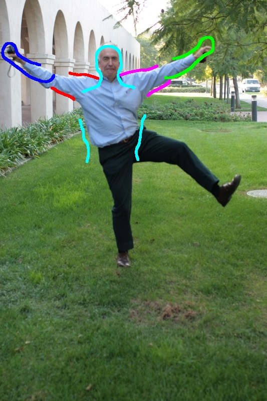
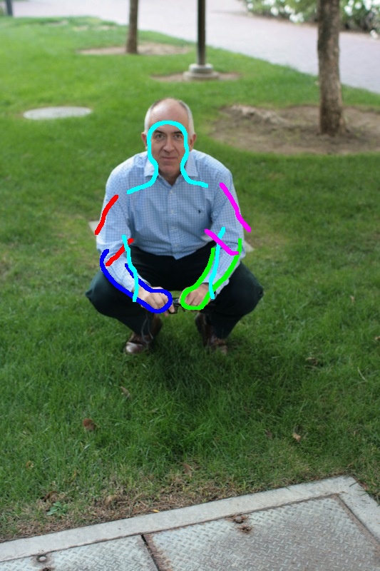
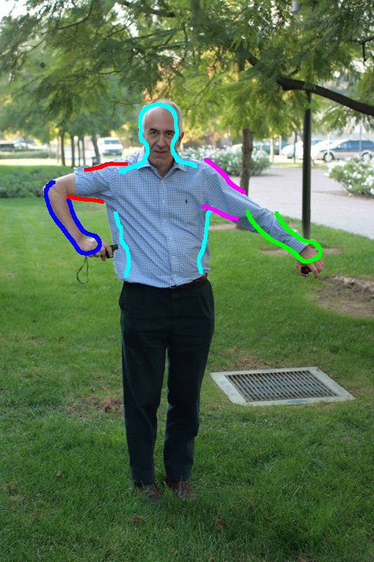
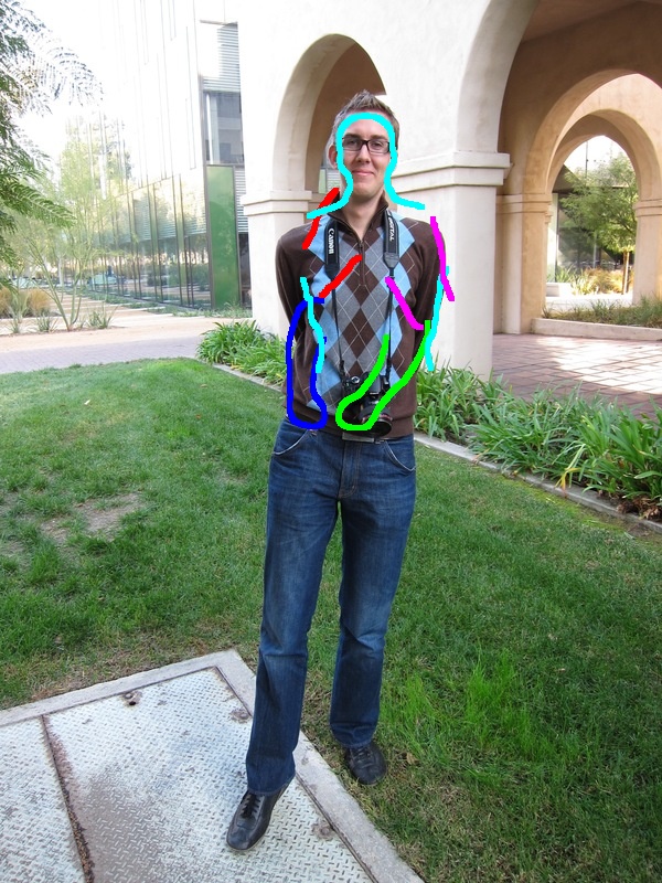
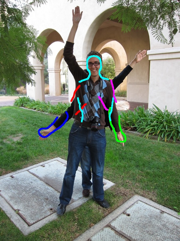
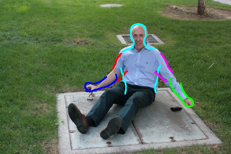
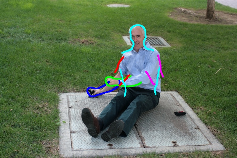
Stepping beyond these demonstrations of algorithmic soundness, benchmarking was extended to real-world imagery. We have applied the trained meta model with all cues to all 63 images in the INIPURE database. The results were inspected and the images divided in two categories, 17 complete failures and 46 acceptable matches. Some of the latter are depicted in Fig. 5, full results are provided as additional material. The optimal posture estimate for the canonical meta model has been overlaid to the query images, qualitatively demonstrating that inferred posture comes close to human intuition.

Increased visual complexity will cause posture analysis to become less precise and might even evoke partially wrong estimation results like in figs. 13c and 13d.

With the acceptable matches, we further investigated the contributions of the meta model’s single cues to the matching success. To that end, let meta model $\mathbf{M}_{\text{meta}_{\mathcal{C}}}$ be assembled from the canonical input sequence introduced above. Further, assume that use of shape and color features in $\mathbf{M}_{\text{meta}_{\mathcal{C}}}$ can selectively be controlled via ‘switches’ $\tilde{S}$, resp. $\tilde{C}$. Other switches are deemed available for Gabor-based limb pre-detection ($\tilde{G}$), search space restriction by $\theta_{typ,(\cdot)}$ ($\tilde{R}$), application of stimulus maps ($\tilde{M}$), and image enhancement by chromatic adaptation ($\tilde{A}$), allowing to activate/deactivate them on demand. The switch configuration variable $\mathcal{C}$ shall represent the set of engaged switches; for instance, $\mathcal{C}=\{\tilde{S},\tilde{G},\tilde{R},\tilde{C},\tilde{M},\tilde{A},\}$ indicates that $\mathbf{M}_{\text{meta}_{\mathcal{C}}}$’s capabilities are in full function, while $\mathcal{C}=\{\}$ identifies an inactivated meta model that becomes powerless in matching attempts.

(a)

(b)

(c)

(d)

(e)

(f)

Figure 5: Examples of successful posture matching by the learned model (top row) and posture mimicry performed by the NAO robot. (bottom row).

As the following statistics serve for system intrinsic comparison, it is reasonable to defer overly complex outlier cases and focus on the $N_{\text{B}}$ image subset during evaluation of the average $\mu_{\mathcal{C}}$ and standard deviation $\sigma_{\mathcal{C}}$ of $E_{\mathcal{C},b}$. Table II shows that pure shape information does not remotely suffice to ensure reliable posture inference (row 1), as background clutter induces a large number of false positive shape elements, causing imprecise (excessively large mean) and unstable (large standard deviation) results. By adding Gabor-based limb pre-detection routines (row 2), matching precision increases, yet, as indicated by the large standard deviation, remains unstable.

Locking body part rotation of all pre-detected meta limbs $i$ to $\theta_{typ,i}$ (row 3) not only speeds up the matching process but also allows to circumnavigate a range of false local optima. Nevertheless, obtained results are still far from being useful for reliable posture analysis. Exploiting color information (row 4) further increases systemic performance. By activating the stimulus maps (row 5), both mean error and standard deviation show another sudden drop and registration quality increases significantly. Switching on chromatic adaptation (row 6) additionally boosts matching quality by allowing for more reliable color analysis. Wrapping up, tbl. II clearly demonstrates sophisticated cue fusion to be an inevitable mainstay of successful meta model registration in significantly complex real-world situations. Note that the above results were achieved using a ‘well-behaved’ image subset for system intrinsic testing. Stepping to the unbiased image set with $N_{B}$=63 images, including all outlier cases, $\mu_{\mathcal{C}}$ becomes 25 pixels, while $\sigma_{\mathcal{C}}$ takes on a value of 30 pixels (with all switches active).

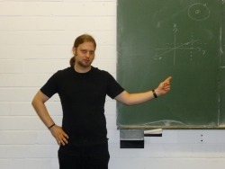
To get a more comparative overview of the performance of our solution in publicly available ‘real-world’ scenarios, we tested our routines on the ‘Perona November 2009 Challenge’ (Perona, 2012) dataset. While performing posture estimation on this less complex image ensemble, poses were correctly recognized on 10 images out of 32, yielding $R_{ok}=31.25$. Here $R_{ok}$ defines the percentage of ‘correctly’ recognized poses by means of human intuition. While this measure is no true quantitative value, it allows to check the estimation performance of our system on external image benchmarks without the necessity for extensive pose tagging. As our system learns from a single subject and has to generalize from autonomously acquired knowledge (compared to massive training found in standard posture estimation approaches) this value seems quite acceptable. Some matches are shown in 4, full results in the additional material, figs. 14 through 15. For the INIPURE dataset $R_{ok}$ becomes equal to $69.84$.

V-D Timing considerations

Calculations were done on an AMD Phenom™ II X4 965, 3.4 GHz unit with 4 GB of RAM, and an NVIDIA^® GeForce^®9800 GT graphics adapter.

Model	frames	seconds total	seconds per frame
0	200	42	0.21
1	200	46	0.23
2	200	58	0.29
3	600	80	0.13
4	185	42	0.22
5	109	29	0.26
6	270	60	0.22
7	232	56	0.24
8	207	49	0.24
9	193	50	0.26
10	249	58	0.23
11	331	77	0.23
12	248	53	0.21
13	379	75	0.19
14	115	28	0.24
15	75	21	0.27
16	460	83	0.18
			$\oslash=$0.23

TABLE III: Construction times for sequence-specific models

Tbl. III shows processing times (third column) are logged for each sequence-specific model from initial motion segmentation to final PS generation. Normalization by the number of frames in each sequence yields comparable per-frame figures (fourth column), whose mean of $\leq 0.25$ seconds per frame indicates that sequence-specific upper body models can be learned reasonably fast.

With that, it becomes interesting to analyze meta model construction timings; necessary figures are logged while performing above permutation tests: be $T(\mathbf{M}_{\text{meta}_{r}})$ the time (in seconds) it takes to assemble $\mathbf{M}_{\text{meta}_{r}}$ from row $r$ of the permutation table. As meta model construction periods linearly depend on the number of integrated, sequence-specific models, the mean of all observed $T(\mathbf{M}_{\text{meta}_{r}})$, $r=0,\ldots,N_{\text{T}}-1$ is divided by $N_{\text{M}}$, such that $T_{\text{meta}}$ expresses the average meta model construction time per integrated body pattern. Given the above hardware/software configuration, values of $T_{\text{meta}}\approx$ 45 seconds per integrated model are achieved, allowing to assemble meta models swiftly, even for growing $N_{\text{M}}$, as meta model construction time is linear in the number of integrated models. Eventually, assume that meta model registration timings have been logged for all ‘non-outlier’ experiments. Finding the mean of the recorded figures, the meta model matching cycle can be stated to consume 178 seconds per image. This value could be improved with additional GPUs.

Figure 6: NAO’s mimicking behavior

V-E Controlling the NAO robot device

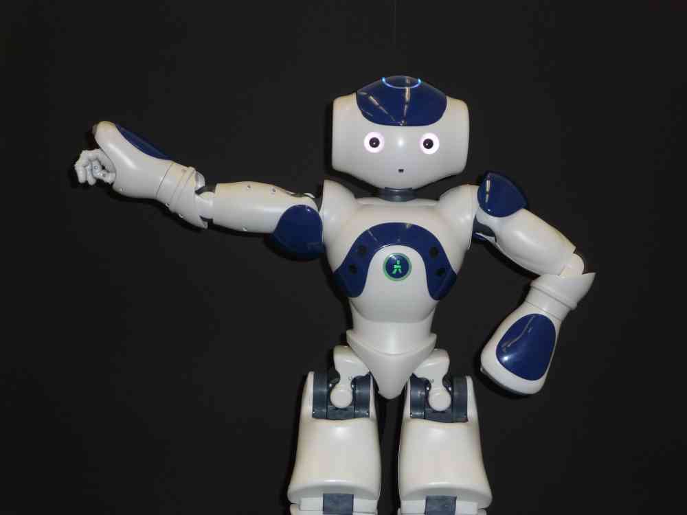
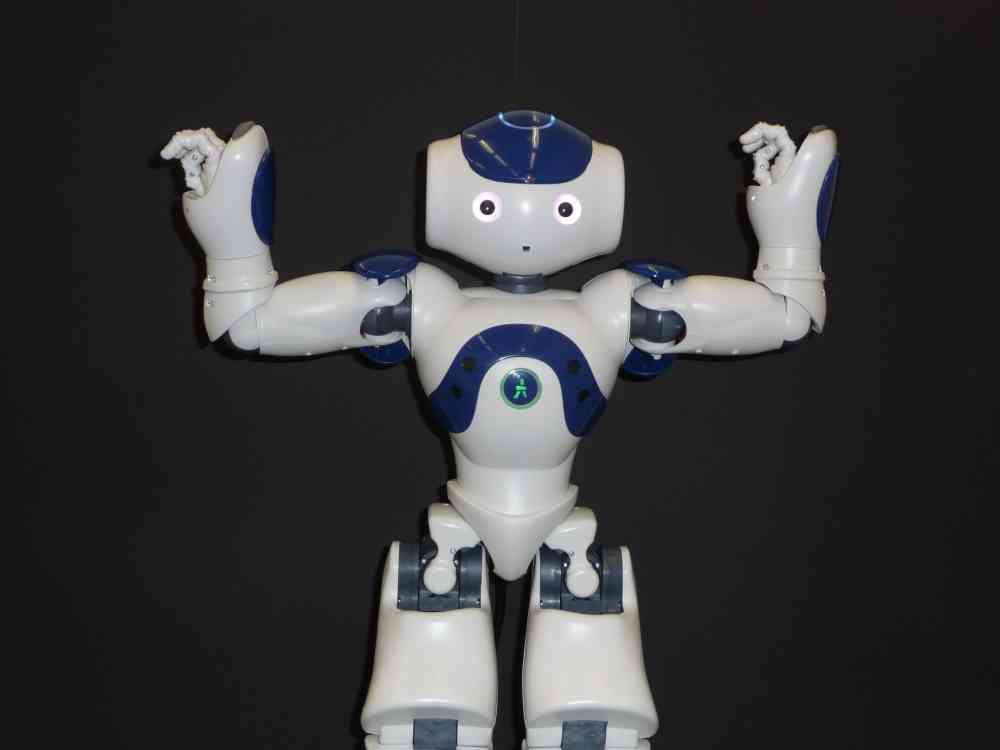
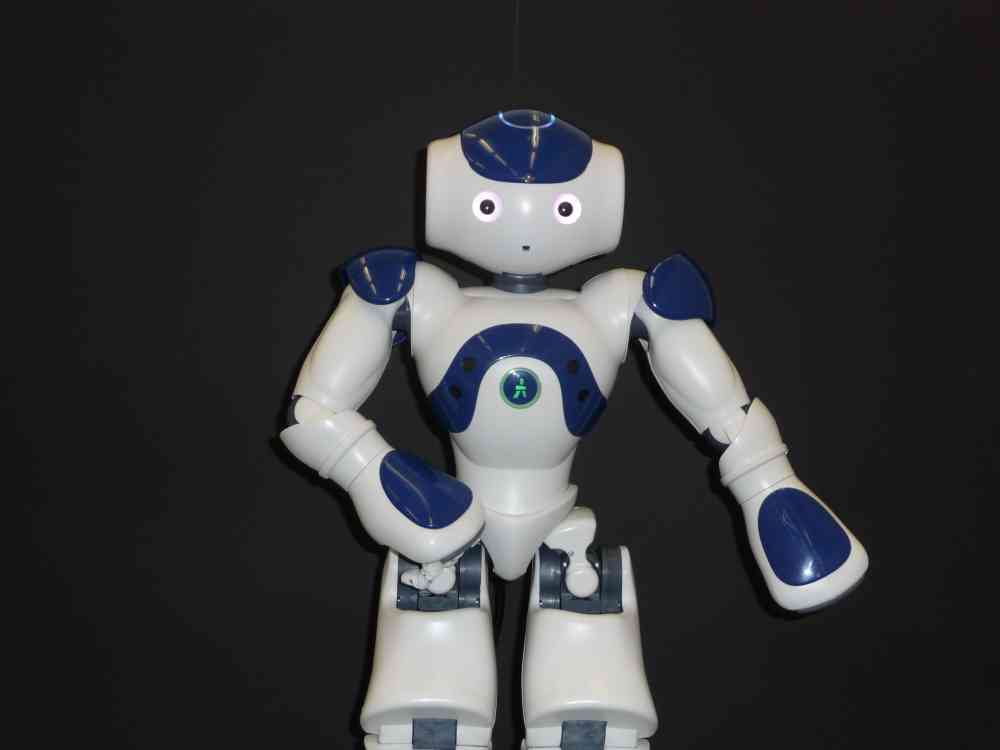
For the VBMC framework proposed in this paper, our experiments demonstrate good generalization performance in weakly constrained scenarios. To demonstrate another use, we have implemented a behavior on a NAO robot device (manufactured by Aldebaran Robotics), which uses the learned meta model to compare an externally observed posture to its own posture and then making appropriate movements to assume the same posture, thus mimicking a human example.

Using the NAOqi framework, the robot’s kinematic configuration can be controlled. From NAOqi’s access to NAO’s kinematics, an upper body skeleton can be assembled that reliably traces the robot’s posture changes. Assuming fronto-parallel motion patterns under orthographic projection, the single ‘bones’ of the skeleton are expected to move parallel to the image plane, relative to which the rotation axes of the connecting joints should remain perpendicular. Therefore, the 3D skeleton is projected to the image plane by dropping depth information. The resulting skeletal footprint $F(\mathbf{P})$ yields a good 2D approximation of NAO’s effective 3D pose $\mathbf{P}$, given that foreshortening is kept at bay (ensured manually). Each projection is augmented with the parameters of the 3D configuration it approximates; this way, NAOqi’s actuator control routines can later be invoked to restore 3D posture corresponding to any particular skeletal footprint. With these preparations, NAO is guided manually through a range of fronto-parallel, collision-free upper body poses that are deemed typical for human beings. Footprints for each of the trained poses are sampled and stored, yielding an ample footprint repository $\mathcal{R}$.

Now, if NAO is actuated to take on ‘T-like’ posture $\mathbf{P}_{\text{T}}$; a ‘snapshot’ of this scenario is provided by $\mathbf{I}_{\text{T}}(\mathbf{x})$. $\mathbf{M}_{\text{meta}}$ is matched to $\mathbf{I}_{\text{T}}(\mathbf{x})$; all cues other than shape are turned off in this registration process, realizing that NAO’s appearance (w. r. t. color and texture) does not even remotely resemble the human look encoded in $\mathbf{M}_{\text{meta}}$. Thus, stepping beyond shape features would only hamper reliable model registration here. Following successful matching, structural correspondences between the matched meta model and the skeleton encoded by $F(\mathbf{P}_{\text{T}})$ are learned. Assuming persistence of the established correspondences allows to find, for any meta model configuration $\mathcal{L}$, the most similar skeletal footprint in $\mathcal{R}$.

To actually mimic posture observed in an image $\mathbf{I}_{\text{Q}}(\mathbf{x})$, the above relations come in handy: let $\mathcal{L}^{*}$ represent the globally optimal posture inferred by matching $\mathbf{M}_{\text{meta}}$ to $\mathbf{I}_{\text{Q}}(\mathbf{x})$. Let further skeletal footprint $F^{*}(\mathbf{P}^{*})\in\mathcal{R}$ be the one most similar to $\mathcal{L}^{*}$. The observed upper body pose is then replicated by sending parameters encoded in $\mathbf{P}^{*}$ to NAOqi, which in turn actuates NAO as to take on the desired kinematic configuration. For a graphical overview of the described posture mimicking cycle, see fig. 6.

Due to the discrete nature of footprints collected in $\mathcal{R}$, posture mimicking results will necessarily be an approximation to $\mathcal{L}^{*}$. In addition, NAO’s hardware limits the spectrum of natural upper body poses that can be emulated (for instance, folding the robot’s arms seems physically impossible). Notwithstanding these limitations, Fig. 5 qualitatively demonstrate the proposed framework’s effectiveness in mirroring posture observed in real-world footage.

VI Comparison with supervised approaches

We also challenged our system with publicly available benchmarks like the ‘Buffy Stickmen’ (Ferrari et al., 2012) image ensemble. Here, recognition rates were negligible compared to contemporary posture estimators including, for instance, (Eichner et al., 2012). In fact, our system occasionally found correct postures, yet these data didn’t suffice to set up meaningful statistics. However, such behavior was expected: images in the ‘Buffy’ set are extremely complex, showing strong illumination, pose, and scale variations. As our system had to learn posture estimation from scratch without human guidance, it can by no means compete with contemporary pose estimation solutions like (Eichner et al., 2012) who make intense use of manual training and inject significant a priori knowledge into their system (for instance, by utilizing pre-made upper body detectors).

The current state of the art in human pose estimation in still images is defined by Toshev and Szegedy (2014). The system consists of a body detector, which preprocesses all images. Afterwards, a cascade of convolutional neural networks is trained on 11000 images from the FLIC Sapp and Taskar (2013) and Leeds Johnson and Everingham (2011) datasets. Each of these images is manually annotated with the position of 10 upper body joints. Data augmentation by mirroring and crop box variation yields a total of 12 million training images.

Like in all feedforward neural network approaches, evaluation of a single image is extremely fast at 0.1s on a 12 core CPU. Training is more laborious and takes some 24 days on 100 “workers” (presumably combined CPU/GPU machines). Success rates are around 80% for arms. The corresponding numbers for our system are 4253 video frames, none of which is annotated for training. Training time is 16 minutes on a PC, and evaluation of a single still image takes about 3 minutes. It is successful in 70% of the cases on our own dataset, and 31% on the Perona challenge.

Clearly, our system cannot match the performance of supervised systems but it demonstrates a reasonable learning success in a different setting with much fewer ressources. Furthermore, enhancing our matching with preprocessing by a body detector would certainly yield much better results, especially on the multiple person images. The goal of our experimentation was to show the capabilities and shortcomings of a body model learned in an unsupervised way.

VII Conclusion

The promising results above allow to state that OC principles might well be used to alleviate the obstructive need for human supervision that plagues conventional HPE/HMA solutions. Our system learns conceptual representations of the upper human body in a completely autonomous manner, the experiments show that the resulting meta model achieves perceptually acceptable posture inference in moderately complex scenes. Nevertheless, much work remains to be done: one idea would be to replace our motion segmentation scheme; switching to methods found, e. g., in (Kumar et al., 2008) could allow for system training in scenarios of increased complexity. Beyond that, parallelization techniques show potential in boosting model matching; avoiding registration jitter in the learning stage would probably result in improved Gabor models for the single meta limbs.

Acknowledgments

This work was funded by the DFG in the priority program “Organic Computing” (MA 697/5-1, WU 314/5-2, WU 314/5-3). We thank our colleagues at the Institut für Neuroinformatik for posing for the testing data.

VIII References

Additional Material

(a) Original image

(b) Results of backprojecting information from $\mathcal{H}_{\text{meta},\text{torso}}$ to Fig. 7a.

Figure 7: Exemplary backprojection map, color encoding is in heat map style, as indicated by the color reference bar below Fig. 7b.

(a) Original image

(b) Gabor cue map for Fig. 8a

Figure 8: Exemplary Gabor cue map for the meta torso: for visual convenience, normalization to $[0;,1]$ has been applied in the right image; generic heat map color encoding is used, black regions represent ‘forbidden’ torso locations. The torso detection corresponding to the most pronounced minimum in Fig. 8b has been overlaid to Fig. 8a (green outline).

(a) Low entropy

(b) High entropy

Figure 9: Visualized entropy states: the depicted color similarity maps $U_{R_{\text{torso}},\gamma_{\text{torso}}}(\mathbf{x})$ are calculated for the original input image in Fig. 7a; color encoding is in heat map style.

(a)

(b)

(c)

(d)

(e)

(f)

Figure 10: Posture estimation results (sheet A)

(a) Original input image

(b) $C_{\text{torso}}(\mathbf{x})$ for Fig. 11a

(c) After chromatic adaptation

(d) $C_{\text{torso}}(\mathbf{x})$ for Fig. 11c

Figure 11: Exemplary chromatic adaptation results: the backprojection maps’ color encoding is in heat map style; observe the significant improvement achieved through chromatic adaptation.

(a)

(b)

(c)

(d)

Figure 12: Posture estimation results (sheet K)

(a)

(b)

(c)

(d)

(e)

(f)

Figure 13: Posture estimation results (sheet B)

(a)

(b)

(c)

(d)

(e)

(f)

(g)

(h)

Figure 14: Posture estimation results, ‘Perona November 2009 Challenge’, by courtesy of Pietro Perona, (sheet A)

(a)

(b)

Figure 15: Posture estimation results, ‘Perona November 2009 Challenge’, by courtesy of Pietro Perona, (sheet D)

References

- Besl and McKay (1992) Besl, P. J., McKay, N. D., 1992. A method for registration of 3-D shapes. Trans. PAMI 14 (2), 239–256.
- Boykov and Jolly (2001) Boykov, Y., Jolly, M.-P., 2001. Interactive graph cuts for optimal boundary and region segmentation of objects in N-D images. In: Proc. ICCV. Vol. 1. pp. 105–112.
- Boykov and Kolmogorov (2004) Boykov, Y., Kolmogorov, V., 2004. An experimental comparison of min-cut/max-flow algorithms for energy minimization in vision. Trans. PAMI 26 (9), 1124–1137.
- Christoudias et al. (2002) Christoudias, C. M., Georgescu, B., Meer, P., 2002. Synergism in low level vision. In: Proc. ICPR. Vol. 6. pp. 150–155.
- Dempster et al. (1977) Dempster, A. P., Laird, N. M., Rubin, D. B., 1977. Maximum likelihood from incomplete data via the EM algorithm. Journal of the Royal Statistical Society B 39 (1), 1–38.
- Eichner et al. (2012) Eichner, M., Marin-Jimenez, M., Zisserman, A., Ferrari, V., 2012. 2d articulated human pose estimation and retrieval in (almost) unconstrained still images. IJCV 99, 190–214.
- Elgammal et al. (2009) Elgammal, A., Muang, C., Hu, D., 2009. Skin detection. In: Li, S. Z., Jain, A. K. (Eds.), Encyclopedia of Biometrics. Springer, pp. 1218–1224.
- Eriksen (2006) Eriksen, R. D., 2006. Image Processing Library 98. www.mip.sdu.dk/ipl98/, version 2.20.
- Felzenszwalb and Huttenlocher (2000) Felzenszwalb, P. F., Huttenlocher, D. P., 2000. Efficient matching of pictorial structures. In: Proc. CVPR. pp. 66–73.
- Felzenszwalb and Huttenlocher (2005) Felzenszwalb, P. F., Huttenlocher, D. P., 2005. Pictorial structures for object recognition. IJCV 61 (1), 55–79.
- Ferrari et al. (2012) Ferrari, V., Eichner, M., Marin-Jimenez, M. J., Zisserman, A., 2012. Buffy stickmen v3.01 annotated data and evaluation routines for 2d human pose estimation. http://www.robots.ox.ac.uk/~vgg/data/stickmen/.
- Ferrari et al. (2008) Ferrari, V., Marín-Jiménez, M., Zisserman, A., 2008. 2D human pose estimation in TV shows. In: Proc. Dagstuhl Seminar on Statistical and Geometrical Approaches to Visual Motion Analysis. Vol. 5604 of LNCS. Springer, pp. 128–147.
- Finlayson and Süsstrunk (2000) Finlayson, G. D., Süsstrunk, S., 2000. Spectral sharpening and the Bradford transform. In: Color Imaging Symposium. pp. 236–243.
- Fischler and Elschlager (1973) Fischler, M. A., Elschlager, R. A., 1973. The representation and matching of pictorial structures. IEEE Transactions on Computers 22 (1), 67–92.
- Frey and Dueck (2007) Frey, B. J., Dueck, D., 2007. Clustering by passing messages between data points. Science 315, 972–976.
- Gavrila (1999) Gavrila, D. M., 1999. The visual analysis of human movement: a survey. CVIU 73 (1), 82–98.
- Golub and Van Loan (1996) Golub, G. H., Van Loan, C. F., 1996. Matrix Computations, 3rd Edition. The Johns Hopkins University Press.
- Hariharan et al. (2012) Hariharan, B., Malik, J., Ramanan, D., 2012. Discriminative decorrelation for clustering and classification. In: Proc. ECCV. Springer, pp. 459–472.
- Hsu et al. (2008) Hsu, E., Mertens, T., Paris, S., Avidan, S., Durand, F., 2008. Light mixture estimation for spatially varying white balance. ACM Transactions on Graphics 27 (3), 70:1–70:7.
- Johnson and Everingham (2011) Johnson, S., Everingham, M., June 2011. Learning effective human pose estimation from inaccurate annotation. In: Computer Vision and Pattern Recognition (CVPR), 2011 IEEE Conference on. pp. 1465–1472.
- Kameda and Minoh (1996) Kameda, Y., Minoh, M., 1996. A human motion estimation method using 3-successive video frames. In: Proc. Intl. Conf. on Virtual Systems and Multimedia. pp. 135–140.
- Kanaujia et al. (2007) Kanaujia, A., Sminchisescu, C., Metaxas, D., 2007. Semi-supervised hierarchical models for 3D human pose reconstruction. In: Proc. CVPR. pp. 1–8.
- Krahnstoever (2003) Krahnstoever, N., 2003. Articulated models from video. Ph.D. thesis, Pennsylvania State University.
- Kumar et al. (2008) Kumar, M. P., Torr, P. H. S., Zisserman, A., 2008. Learning layered motion segmentations of video. IJCV 76 (3), 301–319.
- Kumar et al. (2010) Kumar, M. P., Torr, P. H. S., Zisserman, A., 2010. OBJCUT: Efficient segmentation using top-down and bottom-up cues. Trans. PAMI 32 (3), 530–545.
- Lades et al. (1993) Lades, M., Vorbrüggen, J. C., Buhmann, J., Lange, J., von der Malsburg, C., Würtz, R. P., Konen, W., 1993. Distortion invariant object recognition in the dynamic link architecture. IEEE Transactions on Computers 42 (3), 300–311.
- Lan and Huttenlocher (2005) Lan, X., Huttenlocher, D. P., 2005. Beyond trees: common-factor models for 2D human pose recovery. In: Proc. ICCV. pp. 470–477.
- Lee and Grauman (2009) Lee, Y. J., Grauman, K., 2009. Shape discovery from unlabeled image collections. In: Proc. CVPR. IEEE, pp. 2254–2261.
- Mannan (2008) Mannan, F., 2008. Interactive image segmentation, project work. www.cs.mcgill.ca/~fmanna/ecse626/project.htm.
- Mardia and Jupp (2000) Mardia, K. V., Jupp, P. E., 2000. Directional Statistics. Wiley.
- Margulis (2006) Margulis, D., 2006. Photoshop LAB Color: The Canyon Conundrum and Other Adventures in the Most Powerful Colorspace. Peachpit Press.
- Moeslund et al. (2006) Moeslund, T. B., Hilton, A., Krüger, V., 2006. A survey of advances in vision-based human motion capture and analysis. CVIU 104 (2), 90–126.
- Montojo (2009) Montojo, J., 2009. Face-based chromatic adaptation for tagged photo collections.
- Mori et al. (2004) Mori, G., Ren, X., Efros, A. A., Malik, J., 2004. Recovering human body configurations: combining segmentation and recognition. In: Proc. CVPR. pp. 326–333.
- Navaratnam et al. (2006) Navaratnam, R., Fitzgibbon, A. W., Cipolla, R., 2006. Semi-supervised learning of joint density models for human pose estimation. In: Proc. BMCV. Vol. 2. pp. 679–688.
- Perona (2012) Perona, P., 2012. Perona november 2009 challenge. http://groups.inf.ed.ac.uk/calvin/articulated_human_pose_estimation_code/downloads/perona-nov09.tgz.
- Pfister et al. (2013) Pfister, T., Charles, J., Zisserman, A., 2013. Large-scale learning of sign language by watching tv (using co-occurrences). In: Proc. BMVC. pp. 1–20.
- Poggio and Bizzi (2004) Poggio, T., Bizzi, E., 2004. Generalization in vision and motor control. Nature 431 (7010), 768–774.
- Poppe (2007) Poppe, R., 2007. Vision-based human motion analysis: an overview. CVIU 108 (1–2), 4–18.
- Ramanan et al. (2006) Ramanan, D., Forsyth, D. A., Barnard, K., 2006. Building models of animals from video. Trans. PAMI 28 (8), 1319–1334.
- Ramanan et al. (2007) Ramanan, D., Forsyth, D. A., Zisserman, A., 2007. Tracking people by learning their appearance. Trans. PAMI 29 (1), 65–81.
- Roberts et al. (2007) Roberts, T. J., McKenna, S. J., Ricketts, I. W., 2007. Human pose estimation using partial configurations and probabilistic regions. IJCV 73 (3), 285–306.
- Ross et al. (2010) Ross, D. A., Tarlow, D., Zemel, R. S., 2010. Learning articulated structure and motion. IJCV 88 (2), 214–237.
- Rusinkiewicz and Levoy (2001) Rusinkiewicz, S., Levoy, M., 2001. Efficient variants of the ICP algorithm. In: Proc. 3DIM. pp. 145–152.
- Sapp and Taskar (2013) Sapp, B., Taskar, B., June 2013. Modec: Multimodal decomposable models for human pose estimation. In: The IEEE Conference on Computer Vision and Pattern Recognition (CVPR). pp. 3674–3681.
- Shi and Malik (2000) Shi, J., Malik, J., 2000. Normalized cuts and image segmentation. Trans. PAMI 22 (8), 888–905.
- Shotton et al. (2008) Shotton, J., Blake, A., Cipolla, R., 2008. Multiscale categorical object recognition using contour fragments. Trans. PAMI 30 (7), 1270–1281.
- Sigal and Black (2006a) Sigal, L., Black, M. J., 2006a. Measure locally, reason globally: occlusion-sensitive articulated pose estimation. In: Proc. CVPR. pp. 2041–2048.
- Sigal and Black (2006b) Sigal, L., Black, M. J., 2006b. Predicting 3D people from 2D pictures. In: Proc. AMDO. Vol. 4069 of LNCS. Springer, pp. 185–195.
- Sigal et al. (2003) Sigal, L., Isard, M., Sigelman, B. H., Black, M. J., 2003. Attractive people: assembling loose-limbed models using non-parametric belief propagation. In: Proc. NIPS. MIT Press.
- Sminchisescu and Triggs (2003) Sminchisescu, C., Triggs, B., 2003. Kinematic jump processes for monocular 3D human tracking. In: Proc. CVPR. pp. 69–76.
- Song (2003) Song, Y., 2003. A probabilistic approach to human motion detection and labeling. Phd thesis, California Institute of Technology, Pasadena, California.
- Stenger et al. (2004) Stenger, B., Thayananthan, A., Torr, P. H. S., Cipolla, R., 2004. Hand pose estimation using hierarchical detection. In: Proc. ECCV workshop on HCI. Vol. 3058 of LNCS. Springer, pp. 105–116.
- Swain and Ballard (1991) Swain, M. J., Ballard, D. H., 1991. Color indexing. IJCV 7 (1), 11–32.
- Tomasi and Kanade (1991) Tomasi, C., Kanade, T., 1991. Shape and motion from image streams: a factorization method – 3 – detection and tracking of point features. Technical report, Carnegie Mellon.
- Toshev and Szegedy (2014) Toshev, A., Szegedy, C., June 2014. Deeppose: Human pose estimation via deep neural networks. In: 2014 IEEE Conference on Computer Vision and Pattern Recognition. pp. 1653–1660.
- Veksler (1999) Veksler, O., 1999. Efficient graph-based energy minimization methods in computer vision. Ph.D. thesis, Cornell.
- von der Malsburg (2008) von der Malsburg, C., 2008. The organic future of information technology. In: Würtz, R. P. (Ed.), Organic Computing. Springer, pp. 7–24.
- von Luxburg (2007) von Luxburg, U., 2007. A tutorial on spectral clustering. Statistics and Computing 17 (4), 395–416.
- Wallach (2004) Wallach, H. M., 2004. Conditional random fields: an introduction. Technical report MS-CIS-04-21, Univ. of Pennsylvania.
- Walther (2011) Walther, T., 2011. Human motion analysis based on organic computing principles. Ph.D. thesis, Ruhr-Universität Bochum.
- Walther and Würtz (2010) Walther, T., Würtz, R. P., 2010. Learning generic human body models. In: Proc. AMDO. Vol. 6169 of LNCS. Springer, pp. 98–107.
- Yan and Pollefeys (2006) Yan, J., Pollefeys, M., 2006. Automatic kinematic chain building from feature trajectories of articulated objects. In: Proc. CVPR. pp. 712–719.
- Yan and Pollefeys (2008) Yan, J., Pollefeys, M., 2008. A factorization-based approach for articulated nonrigid shape, motion and kinematic chain recovery from video. IEEE Trans. PAMI 30 (5), 865–877.
- Yang and Ramanan (2013) Yang, Y., Ramanan, D., 2013. Articulated human detection with flexible mixtures of parts. Trans. PAMI 35 (12), 2878–2890.
- Zelnik-Manor and Perona (2004) Zelnik-Manor, L., Perona, P., 2004. Self-tuning spectral clustering. In: Proc. NIPS. pp. 1601–1608.