Bayesian truncation errors in chiral effective field theory: nucleon-nucleon observables
Abstract
Chiral effective field theory (EFT) predictions are necessarily truncated at some order in the EFT expansion, which induces an error that must be quantified for robust statistical comparisons to experiment. In previous work, a Bayesian model for truncation errors of perturbative expansions was adapted to EFTs. The model yields posterior probability distribution functions (pdfs) for these errors based on expectations of naturalness encoded in Bayesian priors and the observed order-by-order convergence pattern of the EFT. A first application was made to chiral EFT for neutron-proton scattering using the semi-local potentials of Epelbaum, Krebs, and Meißner (EKM). Here we extend this application to consider a larger set of regulator parameters, energies, and observables as a general example of a statistical approach to truncation errors. The Bayesian approach allows for statistical validations of the assumptions and enables the calculation of posterior pdfs for the EFT breakdown scale. The statistical model is validated for EKM potentials whose convergence behavior is not distorted by regulator artifacts. For these cases, the posterior for the breakdown scale is consistent with EKM assumptions.
I Introduction
The scope of ab initio nuclear structure and reactions has increased dramatically due to recent advances in many-body methods Barrett et al. (2013); Hagen et al. (2014); Carlson et al. (2015); Hergert et al. (2016); Barbieri and Carbone (2016); Lee (2016), continued growth in computational power, and new developments in chiral effective field theory (EFT) Epelbaum et al. (2009); Machleidt and Entem (2011); Gezerlis et al. (2014); Epelbaum et al. (2015a); Piarulli et al. (2015); Entem et al. (2017). To properly judge the successes and predictive power of ab initio nuclear theory, however, it is necessary that theory errors be understood. Thus, quantifying the theoretical uncertainties of nuclear calculations has now become a critical task for confronting experiment and theory and for extrapolating to unmeasured phenomena Dobaczewski et al. (2014); Ireland and Nazarewicz (2015); Carlsson et al. (2016).
Uncertainties in chiral EFT predictions arise from three sources Furnstahl et al. (2015a): uncertainty in the input data to which the EFT parameters are fit, errors in the Hamiltonian, and numerical approximations. Here we focus on quantifying the Hamiltonian truncation error as part of the larger BUQEYE program Furnstahl et al. (2015a) of quantifying all uncertainties for EFT predictions. Despite the promise of systematic expansions, uncertainties from truncation have been difficult to estimate and, when provided, generally lack a well-defined statistical interpretation.
In Ref. Furnstahl et al. (2015b), a Bayesian model for truncation errors originally applied to perturbative expansions in quantum chromodynamics Cacciari and Houdeau (2011); Bagnaschi and Jenniches (2014) was adapted to EFTs. The generic assumption is that the EFT provides us with a dimensionless expansion parameter , which is a ratio of scales, and an associated expansion for quantities (usually observables):
| (1) |
Here, is the natural size of , which could be the leading-order estimate , and the s are dimensionless coefficients. For chiral EFT is zero by symmetry, and we have a double expansion in , where is the relative momentum of two scattering nucleons, is the pion mass, and is the EFT breakdown scale. The goal is to estimate the error incurred in the observable by truncating the expansion at order . Note that this does not exclude an asymptotic expansion, but assumes that we truncate while the result is still improving.
In some cases the expansion in Eq. (1) may follow directly from a perturbative EFT expansion of a Lagrangian, i.e., through a sum of Feynman diagrams with powers of coming from a simple power-law dependence on momentum or a mass (such as the pion mass in a chiral perturbation theory expansion). There will also be implicit dependence, often in the form of logarithms, which vary much more slowly. But in other cases, such as EFT for more than one nucleon, the calculations are nonperturbative, and the dependence on momentum or energy will be complicated and nonlinear in general. Nevertheless, if the EFT is working we expect the calculation of to improve systematically as we go to higher orders.
Equation (1) can be interpreted as a summary of that expected systematic improvement. Namely, that the correction term with each successive order is on average a factor smaller than the previous order. For this to be the case, we need the coefficients to be roughly the same size. Because the coefficients are unknown a priori, we treat them as drawn from a random distribution with a characteristic size. This is a realization of the underlying assumption that the naturalness of the low-energy constants (LECs) in the EFT Lagrangian propagates to the expansion for any observable. We have no general proof of this assumption, so we aim to validate it in each application.
In Ref. Furnstahl et al. (2015b) we made a first pass at formalizing and testing the assumptions behind the expansion in Eq. (1), building on an analogous Bayesian analysis applied to perturbative QCD calculations Cacciari and Houdeau (2011); Bagnaschi and Jenniches (2014). We considered various priors for the s, made an application to a small subset of results from Epelbaum, Krebs, and Meißner (here EKM) for neutron-proton () scattering cross sections using their new semi-local potentials Epelbaum et al. (2015b, a), and tested the consistency of assumed expansion parameters, which are associated with the expected breakdown scales of the EFT implementation. Here we revisit the EKM application to further test and generalize those investigations, which will set the stage for extending our model of EFT truncation errors.
We seek to address the following questions:
- 1.
-
2.
The truncation error model of Ref. Furnstahl et al. (2015b) has not yet been applied to other nucleon-nucleon (NN) observables calculated in chiral EFT, such as the differential cross section and various spin observables. How do the coefficient patterns compare for different NN scattering observables, considered both as functions of energy and scattering angle? Are the naturalness assumptions validated for these observables and for all values of the EKM regulator parameter ?
-
3.
An appropriately assigned error band should capture the true value of an observable of the time. How can we utilize known order-by-order results to verify that the error band prescriptions work as advertised? Can information from different observables be treated as independent, and if not, how can we account for their relationships in our analysis? Is there a well-defined “correlation length” in energy or scattering angle beyond which expansion coefficients may be treated as independent of one another?
-
4.
The identification of the expansion parameter , which in turn is based on identifying the scale , is a key element in determining the convergence pattern. Is it consistent to take to be the same scale for every observable? To what extent can we extract , given order-by-order expansions and our naturalness assumptions encoded in a Bayesian model?
In the present work we make progress on all these questions.
In Sec. II, we summarize and extend the relevant formulas from Ref. Furnstahl et al. (2015b). We refer the reader to that article for background on the use of Bayesian statistics in this context, derivations of the formulas we summarize here, and more general references. New results and analysis for the total cross section are given in Sec. III, and other observables are considered in Sec. IV. In Sec. V we perform Bayesian model checking Gelman et al. (2013) by applying a consistency check used in Ref. Furnstahl et al. (2015b) and by calculating posterior probability distribution functions (pdfs) for . Section VI has our summary and outlook. For completeness and convenience, we show explicit formulas regarding the Bayesian model for truncation errors in Appendix A and summarize the notation and formulas used for NN observables in Appendix B. The Supplemental Material sup displays extra figures and data that helped inform our conclusions.
II Formulas
If the EFT expansion in Eq. (1) is truncated at order , then the error induced is , where the scaled, dimensionless parameter that determines the truncation error is
| (2) |
Generally it is only practical to approximate , the error due to the first omitted higher-order terms. For sufficiently small values of , the first omitted term is a good estimate for , but we do not assume this in general.
We use the notation to denote the probability density of given information . Our pdf of interest is : the probability distribution for given the vector of relevant lower-order coefficients that have been calculated, assuming that only higher-order terms contribute to the error and that is to be given from other considerations. The pdf is normalized in terms of the dummy variable , which is implied to be an estimate of contingent on lower-order coefficients .
In contrast to Ref. Furnstahl et al. (2015b), here because it does not provide insight into the convergence pattern of the observables; rather, the LO calculation provides scaling information. Again, because in chiral EFT. Thus the relevant lower-order coefficients in the determination of in chiral EFT are
| (3) |
In the Bayesian framework, the posterior contains the complete information we claim to have about the dimensionless residual . In general, a posterior pdf can have complex structures such as multiple modes, heavy tails, large skewness, etc. Here we can capture most of the information with a small number of degree-of-belief (DoB) intervals.111These are also called “credibility” or “credible” intervals, or “Bayesian confidence intervals”. We use the highest posterior density (HPD) definition of DoB, which is the shortest interval that contains of the area Kruschke (2011); Gelman et al. (2013); Liu et al. (2015). This ensures that the probability density within the DoB is never lower than the density outside. The HPD definition is particularly well suited for skewed posteriors, as we will encounter in Sec. V. Because the that we consider here are unimodal and symmetric about , finding the DoB interval reduces to the inversion problem for , where
| (4) |
Hence, one believes with certainty the true value of the observable lies within of the NkLO prediction. In general, Eq. (4) must be inverted numerically, but simplified results for certain priors and approximations (e.g., that the first omitted term dominates) are possible Furnstahl et al. (2015b).
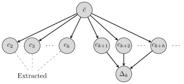
In Ref. Furnstahl et al. (2015b), a statistical model for in terms of the order-by-order coefficients of the EFT expansion was developed. It was assumed that naturalness could be implemented by treating the s as random variables drawn from a shared distribution centered at zero with a characteristic size or upper bound . The coefficients at each order are treated as independent of one another—the value of is the only way that information propagates between orders. These relationships can be encapsulated in a Bayesian network Ben-Gal (2007); Puga et al. (2015), as shown in Fig. 1. The nodes of the graph are random variables and the arrows denote causal relationships between them.
While the topology of Fig. 1 outlines the logic of our model, prescriptions in the form of priors and must be given to make quantitative statistical inferences of . When all we know is that there is an upper bound to the coefficients, an application of maximum entropy Gull (1998); Sivia and Skilling (2006) dictates that the least-informative distribution is uniform for and zero otherwise. Such uniformity is additionally appealing because it can lead to simple, analytic results. This uniform prior was the initial choice of Ref. Cacciari and Houdeau (2011). We employ it in priors we denote as “set A” and “set B” (see Table 1). The analogous prior of “set C” in Table 1 corresponds to the ensemble naturalness assumption of Ref. Schindler and Phillips (2009). This Gaussian prior follows from the maximum-entropy principle assuming knowledge of testable information on the mean and standard deviation of the s Schindler and Phillips (2009):
| (5) |
In addition we require a prior for : . Sets A and C of Table 1 use a log-uniform prior for to reflect unbiased expectations regarding the scale of Jeffreys (1939) (this was the choice in Ref. Cacciari and Houdeau (2011) and Ref. Schindler and Phillips (2009)). Such a prior cannot be normalized for in and is therefore termed an “improper prior”. Limiting the range of through the use of functions permits an examination of the otherwise ill-defined limiting behavior. When marginalizing (i.e. integrating) over , we can express complete ignorance of the scale of by considering the limit of infinite range ( or , see Furnstahl et al. (2015b)), or render the prior more informative through the use of a finite range ( or ). Alternatively, set B employs a log-normal distribution about zero Bagnaschi et al. (2015); Bagnaschi and Jenniches (2014), which sets the scale of with the hyperparameter .
| Set | ||
|---|---|---|
| A | ||
| B | ||
| C |
The general result for implied by Fig. 1 was derived as222We have corrected and simplified here the corresponding equation from Ref. Furnstahl et al. (2015b).
| (6) |
where
| (7) |
If we assume that the first omitted term dominates the truncation error, then Eq. (7) is easily evaluated by the function for any prior, and Eq. (6) reduces to
| (8) |
where as enforced by the function. Error bands made under this assumption are denoted by the prior with a superscript (1), e.g., . Further progress, with or without the first-omitted-term approximation, requires an explicit choice of priors. The relevant equations for this work, such as posteriors and DoB intervals, are contained Appendix A.
III Total NN cross section
Truncation error DoBs were estimated in Ref. Furnstahl et al. (2015b) for the total cross section at laboratory energies of 50, 96, 143, and 200 MeV from results given explicitly in Refs. Epelbaum et al. (2015b, a) using the new R = 0.9 fm EKM potential. In this work we extend these calculations to all of the new potentials and for all energies up to 350 MeV. The first step is to extract the coefficients, defined by Eq. (1), from the order-by-order calculations of the total cross section . Here we choose our reference scale to be the leading-order calculation , so by construction. Other reasonable choices of , such as a higher-order result or the experimental value, do not substantially change the convergence pattern for this observable.
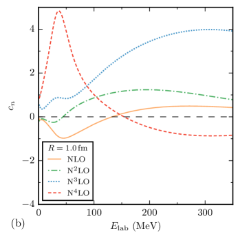
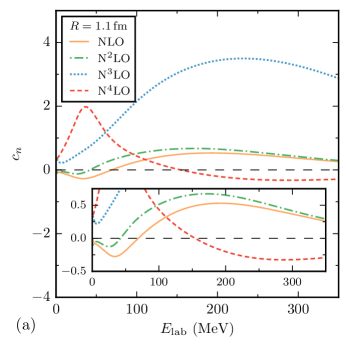
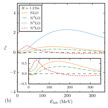
We also need to specify the high-momentum scale . Here we assume that is a given quantity, and adopt the values assumed by EKM. Their choice of MeV (the particular value depending on a regulator parameter ) was based on a rough analysis of residual error plots (“Lepage plots”), validated by the observation that their choices resulted in natural coefficients in the EFT series for scattering cross sections Epelbaum et al. (2015b, a). In Sec. V, we make a statistical analysis of whether the EKM choices of (or nearby values) lead to self-consistent convergence patterns for observables, and explore directly determining a posterior probability distribution for .
Because we have a double expansion in and , we must develop a prescription to define . In Ref. Furnstahl et al. (2015b) we took to be
| (9) |
We expect that at low momenta the expansion will be dominated by powers of and at momenta much higher than it will be dominated by powers of , so the appropriate choice of in each region follows correctly from Eq. (9). However, it is not clear how we should parameterize the crossover region. To avoid cusps at , we choose to replace Eq. (9) by a smooth interpolation function for :
| (10) |
where is a sufficiently high integer (we take here). But we need to examine the behavior at low energies to assess whether the implicit equal weighting of the expansions is justified.
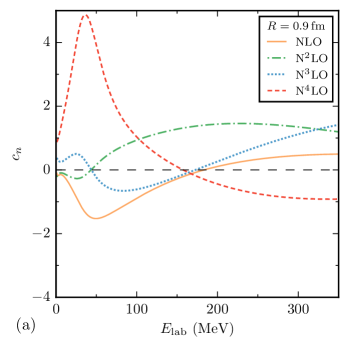
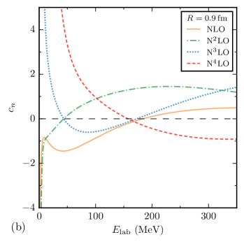
Coefficients – for the total cross section, calculated with the fm potential and MeV, are shown as functions of energy in the left panel of Fig. 2. These include the results for four individual energies from Furnstahl et al. (2015b), but now we can see the global pattern. Except for the coefficient around MeV, the coefficients at any fixed energy follow a distribution with a characteristic size of about one. If were used for all energies instead of Eq. (10), then the coefficients would grow very large as gets small (i.e., as ), as shown in the right panel of Fig. 2. The onset of this behavior in increases with chiral order and, for , is the source of the large coefficient near MeV. This reflects the increasing sensitivity at large order to the relative contribution of the two expansions in the crossover region. We do not yet have a model to address this behavior. If we exclude the crossover region, the underlying assumption of the priors in Table 1 that the coefficients at a given energy are distributed with a characteristic size is validated.
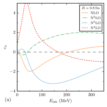
The observable coefficients for the other EKM potentials are shown in Figs. 3 and 4. For each potential we have adopted the value of advocated by EKM: equal to 600 MeV for fm, fm, and fm, 500 MeV for fm, and 400 MeV for fm. We return in Sec. V to consider different choices of .
The general assumption made in constructing a posterior for the truncation error in Ref. Furnstahl et al. (2015b), that the coefficients have a characteristic magnitude or upper bound , is based on the expectation that a well-formulated EFT will have a certain uniformity in the convergence pattern of observables. That is, with each successive order there is a steady convergence implied by the value of the expansion parameter (as shown below, this corresponds with a steady improvement of the prediction for the cross section). For an integrated observable such as the total cross section, we expect this to be particularly manifested. This justifies the use of lower-order results to inform our expectations for higher-order contributions.
The pattern of coefficients for fm shows this uniformity, which is mostly still present for fm and fm. In particular, we see evidence for a characteristic size for the s of order unity (in practice about three). However, the uniformity deteriorates significantly as one progresses to , and fm. This is a consequence of the growing cutoff artifacts at larger values of . As the artifacts become more prevalent, there is a decreased contribution from mid-range pion physics at and , which is counteracted by an increase in the contact terms at and particularly . This reflects a partial integrating-out of pion physics, which takes us closer to a pionless EFT convergence pattern with the dominant contributions at even orders in the expansion.
In Ref. Furnstahl et al. (2015b), we analyzed results only for fm and fm (as reported by EKM) and only at four energies. From this limited sample we concluded that the distribution of s at these energies was consistent with a common for fm, but this was not the case for fm. In particular, the latter case had uniformly small coefficients for N2LO and N4LO, consistent with there being no new short-range contributions at those orders and the regulator greatly reducing the pion tensor-range contribution. Now looking globally at the fm coefficients, we see that N2LO and N4LO stay small for the full range of . If we focus on N2LO in each graph, we see that the trend of the coefficients with energy is quite similar as increases (softening the interaction), but the overall scale decreases monotonically. The situation with N4LO is similar.
Turning to the N3LO coefficients for successive values of , we find a transition from negative and fairly large (order ) at fm to positive and fairly large (order ) at fm and above. fm is the middle of this transition. This is not unnatural, but may reflect a tendency toward overfitting at N3LO (see Ref. Wesolowski and Furnstahl (2017)). Taking all the orders together, the coefficients imply that the convergence pattern for fm and fm, for which regulator artifacts are significant, is not consistent with our statistical model.
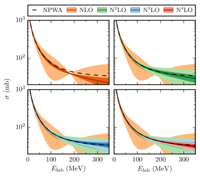
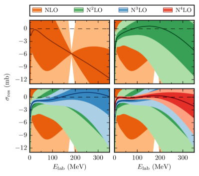
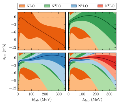
Next we estimate DoB intervals for EFT truncation errors using the extracted coefficients. We apply at each energy the formulas from Sec. II to the coefficients from that energy only. The order-by-order results for the total cross section with fm and prior set (using Eq. (43) or (44)) are shown in Fig. 5. To amplify the patterns, in Fig. 6 and below we plot the residuals with respect to the Nijmegen partial-wave analysis (NPWA) Stoks et al. (1993a), where the residual for a calculated observable is defined as
| (11) |
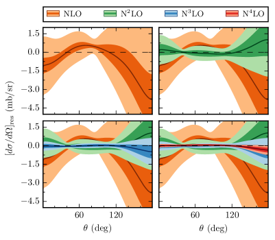
All plots of observables and residuals are shown with solid lines for the calculation at each order, with dark and light shaded bands denoting the 68% and 95% DoB interval for the truncation error at each kinematic point. Note that the errors are not Gaussian, as the 95% bands are not twice the size of the corresponding 68% bands.
The order-by-order convergence of the calculations in Fig. 6 to the NPWA result is clear, but not surprising—the potential was fit to reproduce the NPWA in each partial wave. The pattern of DoB intervals shown in both Figs. 5 and 6 is mostly systematic: the widths tend to increase with , decrease with order, and overlap with preceding order DoBs. Although we used set C for these truncation error estimates on the cross section, the results using set A are similar. See the Supplemental Material sup for plots displaying various error band prescriptions. We return to quantify the effects of prior choice on the success rate of the error bands in Sec. V.
An exception to the systematic and intuitive DoB intervals is for the NLO calculation near 200 MeV, where the intervals vanish. This is because the prior set makes no assumption on the minimum (or maximum) size of , so the only information for the DoB at NLO is the NLO coefficient, which vanishes in that energy range. In Ref. Furnstahl et al. (2015b) we included at NLO, which effectively set a lower limit of . Considering the NLO coefficients over the full energy range, as well as the other coefficients, it is clear that we should use a prior with a non-zero . A more informative, but not too restrictive, choice of (and ) is used in Fig. 7. The DoB intervals at low order are now more plausible while there is no significant difference at the two highest orders.
Of course, it is not enough that the DoB bands are plausible; they should be statistically valid. If our DoB intervals are consistent, we might expect the NPWA line in Fig. 5 or the zero line in Figs. 6 or 7 to lie outside the 68% region roughly 1/3 of the time and outside the 95% region roughly 1/20 of the time. With this in mind, a rough examination of Fig. 7 shows the bands are not ideal: the 95% DoBs appear too large for and , while they are too small for ; the 68% DoBs underestimate the error on the plot; and the DoBs do not perform well at low energies. In Sec. V, we perform a systematic analysis using Bayesian model checking, where we evaluate how well the DoBs predict the subsequent order correction. Section VI concludes with a reassuring proof of concept (Fig. 27), which shows that, on average, our DoBs accurately assess the error of the order-by-order results when compared to NPWA data.
IV Other NN scattering observables
In this section we extend our analysis to other NN scattering observables. For convenience we have collected in the Appendix the relevant notation and formulas we have used, as well as a brief comparison to other notations in the literature. We focus on the differential cross section and a set of the most commonly considered spin observables, namely the analyzing power , polarization transfer coefficients and , and the spin correlation parameters and . Each observable has been generated from LO through N4LO, primarily using the fm potential, which we have seen demonstrates the best convergence pattern. We consider the observables both at fixed energy as a function of angle and at fixed angle as a function of energy.
In Fig. 8, residuals for the differential cross section as a function of scattering angle at fixed MeV for the fm potential are shown as a characteristic example of this observable; other energies display similar characteristics. The detailed order-by-order convergence pattern does not seem to depend on angle, suggesting that it is plausible to describe the convergence statistically.
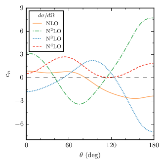
These observations are supported by the plot of coefficients as a function of angle, shown in Fig. 9, for which each order takes a turn at being the largest in magnitude. For this extraction, the leading-order result was taken for ; the results are not sensitive to this choice. The scale of the dimensionless coefficients is roughly uniform at angles less than 150∘ (about four), which is several times larger than the scale for the integrated cross section at this energy. The scale is significantly larger at back angles, where the momentum transfer becomes twice the relative nucleon momentum, which may require a reexamination of the expansion in this region. However, our overall conclusion is that the naturalness assumption, in the form of a characteristic size for the coefficient variations, still holds without integrating over all angles.
For any given spin observable , we assume a natural expansion for the full quantity
| (12) |
which is the probability for a particle to scatter into a solid angle , given that the beam and target particles are polarized in the and directions and the scattered and recoil particle spins are in the and directions, respectively. The dimensionful scale in Eq. (12) is set by the size of the differential cross section, so the natural choice is . That means that the expansion for the spin observable itself is
| (13) |
with no additional prefactor. Below and in the Supplemental Material sup we see that this scaling is consistent with natural ranges for the s.
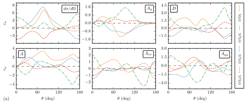
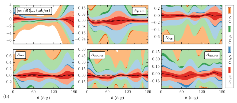
In Fig. 10a we show the extracted coefficients as a function of scattering angle for six scattering observables at MeV, calculated using the potential with fm. The corresponding DoB bands for the residuals at this energy, following the same prescription as applied to the cross sections, are shown in Fig 10b. As already noted, the LO coefficient does not inform our model for truncation errors and so is not shown and is not used for the truncation error posteriors. These figures serve as a representative example; figures showing coefficients and DoB bands for many additional energies are given in the Supplemental Material sup .
Except for constraints on some observables at special angles (e.g., at and at ), the coefficients truly look like independent bounded random functions of the angle, which supports our proposition that a statistical treatment of their behavior is warranted. As with the cross sections, the DoB bands decrease in size systematically and the lower-order bands overlap the higher-order bands. It also appears that, in general, it is not necessary to look at observables integrated over all angles to see a natural EFT convergence pattern. We may therefore apply our statistical model to estimate truncation uncertainties for NN angular observables.
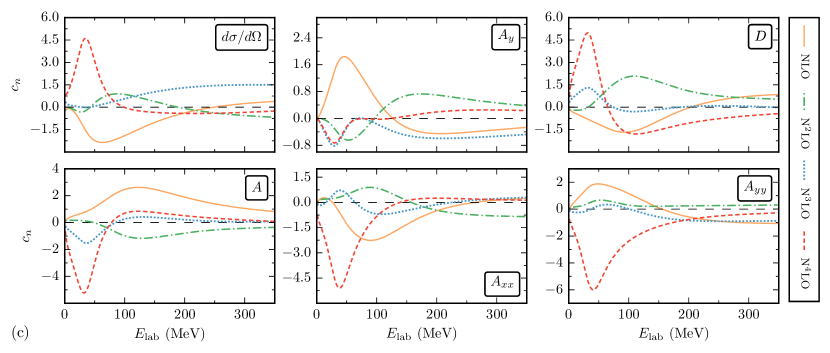
Figure 10c shows coefficients at a fixed angle of as a function of energy. The corresponding DoB intervals are shown in the Supplemental Material sup . Enhanced coefficients in the double-expansion crossover region, noted earlier for the total cross section, are visible in most of the observables. If this region is omitted, the behavior of the coefficients with energies varies with a scale of about 2, with no other systematic patterns apparent.
Thus the observed convergence patterns of NN scattering observables for the EKM interaction with fm, considered as functions of energy or angle, satisfy the statistical model naturalness assumptions implied by Fig. 1. The DoB intervals above 50 MeV derived using prior set C exhibit reasonable patterns (as do those using set A; see Supplemental Material sup ), but do not by themselves validate the statistical model. For that purpose we turn to Bayesian model checking to assess the statistical consistency of all the EKM potentials as well as the sensitivity to the choice of prior sets from Table 1.
V Model Checking
The predictiveness of our statistical model for EFT truncation errors relies on how well our implementation of naturalness aligns with the true convergence pattern exhibited by the EFT. An EFT could fail to exhibit a natural convergence pattern because of regulator artifacts or a poorly chosen . Our prior sets for and , which encode our assumptions about the size of the higher-order coefficients, may also be called into question.
The efficacy of our approach for any given EFT or particular observables predicted by that EFT can be examined using Bayesian model checking Gelman et al. (2013). Here we make use of consistency checks to determine if the DoB intervals behave as advertised. We also investigate the possibility of determining solely from the convergence pattern and the assumption of naturalness.
V.1 Consistency checks
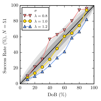
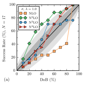
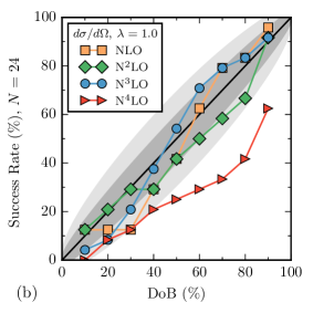
Once a posterior pdf for is determined via Eq. (6), the probability that the truncation error is in a DoB interval follows directly from Eq. (4). If our statistical model for the error is valid, a DoB interval should on average contain the actual next order value of the observable of the time (we use the first-omitted-term approximation in this section). By applying this test for a range of values to a sufficiently large set of observables, we can test for inaccurate models or EFTs with irregular convergence patterns. Such a consistency check provides us with the statistical toolset to analyze the sensitivity to our choice of priors and the consistency of the breakdown scale taken from Ref. Epelbaum et al. (2015b).
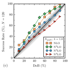
The procedure for creating consistency plots333Calibration plots or curves are other common names for such tools. to implement model checking is as follows Furnstahl et al. (2015b):
-
1.
Choose a set of independent observables for which the next-order calculation is available (not including LO).444In Ref. Furnstahl et al. (2015b) the LO to NLO success rates were included as part of the consistency checks. Because we want to test the convergence pattern only, the LO to NLO success rate is not relevant here, as in the previous sections where we omit .
-
2.
Select a grid of DoB intervals with ranging from 0 to 1.
-
3.
Compute the DoB interval for each observable in the set, using the same priors throughout.
-
4.
For each next-order calculation that is within the DoB interval of the previous order, count one success.
-
5.
Take the number of successes and divide by the total number of observables to get the actual success rate.
-
6.
Plot the success rates versus DoB interval percentage and compare to the ideal result given by a line.
Because we will have a finite number of observables, we expect fluctuations away from the ideal result for a true success rate, as given by the binomial posterior
| (14) |
We apply Bayes theorem with a uniform prior on to convert to a posterior for :
| (15) |
and generalize Eq. (14) to continuous to calculate horizontal 68% and 95% confidence intervals for the DoB percentage, using the HPD prescription (see Sec. II). These become shaded bands in the consistency plots.555In Ref. Furnstahl et al. (2015b) a different procedure yielded bands for given , , and that are reflected about the 45 degree line from the ones here. Additionally, the bands in Furnstahl et al. (2015b) were calculated using equal-tailed credible intervals for DoBs rather than the HPD prescription. Both procedures approach symmetric bands for large .
We can easily evaluate DoB intervals for choices of different from those identified by EKM, which we have adopted so far. We follow Refs. Bagnaschi and Jenniches (2014); Bagnaschi et al. (2015); Furnstahl et al. (2015b) in doing this by introducing a scaling factor to generalize Eq. (1) as
| (16) |
Varying about unity shifts ; in the consistency plots here we consider 20% variations, namely and , with respect to the EKM choice with .
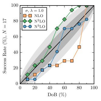
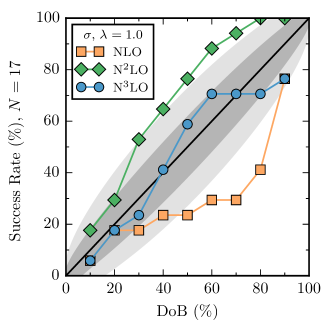
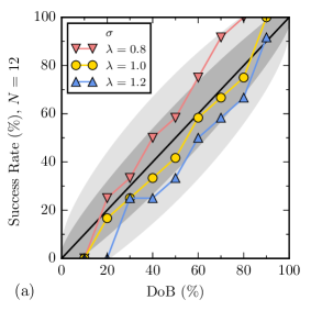
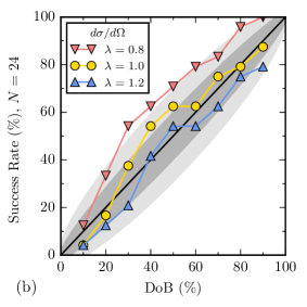
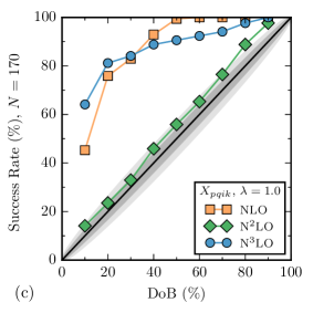
The logic of the remainder of this section is as follows. We begin with a reexamination of the consistency plots for the total cross section, as begun in Figs. 10 and 11 from Ref. Furnstahl et al. (2015b), exploring more energies and stability under prior choice (Figs. 11–13). Next we extend the previous analysis with results from the differential cross section and our selected spin observables (Figs. 14 and 15). Finally, consistency plots of EKM potentials with different regulators are examined (Figs. 16–18), including examples of potentials that fail our analysis (Figs. 19 and 20). For a more extensive survey of our results, see the Supplemental Material sup .
In Fig. 11 we show consistency plots for the total cross section calculated with the fm EKM potential for prior set (recall that the superscript indicates that the truncated error is assumed to be given by the first omitted term). Here, each line averages over the success rate of the , , and error bands in predicting the corresponding next-order contributions at energies MeV. The trends show that for , i.e. MeV, the predicted DoB aligns with the measured success rate to within the uncertainty predicted by Eq. (15). While using data at many values improves the statistics, the independence of the results may be questionable if calculated for too closely spaced kinematic variables. Dependent measurements would cause the gray error bands in Fig. 11 to be too restrictive, so the and lines may be consistent even though they are generally outside the 68% bands (cf. the leftmost plot in Fig. 16). In future work we will model the correlation length in energy using Gaussian processes Rasmussen and Williams (2006); Gelman et al. (2003); Jones et al. (1998) (GPs) to draw more robust conclusions about independence.
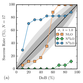
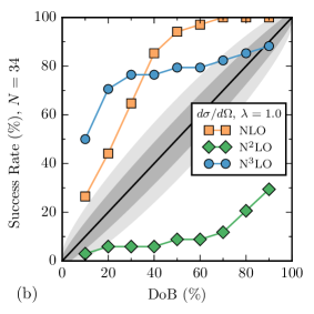
In Fig. 12 we decompose the line of Fig. 11 into the contribution from each individual order, while Fig. 13 shows the same decomposition but using prior set . Given the slight changes between Figs. 12 and 13, as well as similar examples not shown, we conclude that prior choice has little effect on the predictions of EFTs with good convergence patterns. For such an EFT, we expect the predictions to improve with the order of the prediction, because the higher orders contain more information about the pattern of the observable coefficients. This is what we see, with the predictions being fully consistent within the gray bands.
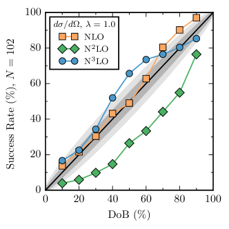
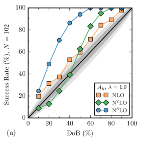
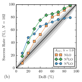
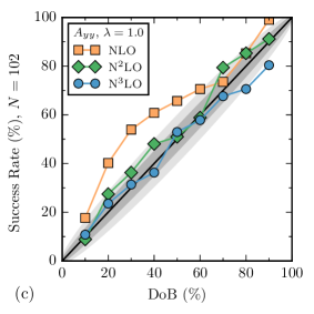

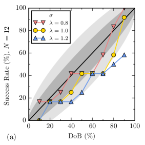
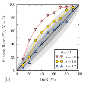
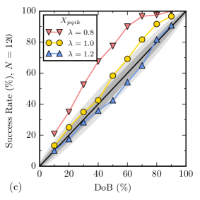
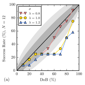
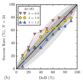
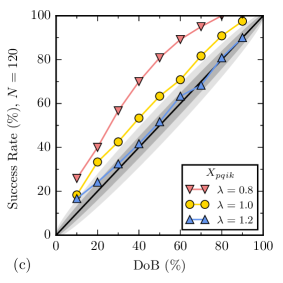
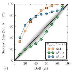
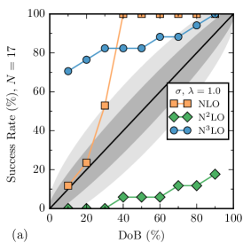
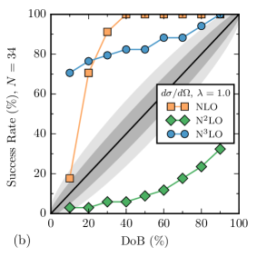
Next we consider angle-dependent observables, which were not analyzed in Ref. Furnstahl et al. (2015b). Each observable is generated using the fm EKM potential with MeV (). Each is evaluated at kinematic points: 17 energies ( MeV, as for ) with 6 angles () for each energy. The prior set used in the analysis is and the plots are decomposed order-by-order. Figure 14 shows a consistency plot for the differential cross section, while Fig. 15 shows, as an example, the individual spin observables , , and . The DoBs consistently underestimate the size of the correction for the differential cross section, but the and DoBs do fairly well. Some of the DoBs for spin observables, such as and , overestimate the higher-order corrections, while the DoB performs well. The and coefficients of and are generally larger than and particularly the coefficients at MeV, while tends to have coefficients that each take turns being the largest.
The spacing in angle and energy may be close enough that the calculations used for the consistency plots are significantly correlated, which will constrain the gray error bands unnecessarily due to the large number of non-independent points. The true impact of this correlation has not yet been quantified and is a topic for future investigation. From the aforementioned plots, we can conclude that although integrating over angles is not necessarily required to ensure a natural convergence pattern of coefficients, some observables do show notable patterns that adversely affect the predictive power of their respective DoBs.
Finally, we return to the topic of EKM potentials with varying regulators, first raised in Sec. III. Thus far we have mainly focused on the fm EKM potential due to its natural convergence pattern compared to the other potentials, as evidenced by Figs. 2–4. Now we relax this focus to gain insight into the effects that regulator choices and their consequent convergence patterns have on the reliability of the error bands generated by this analysis. We also test the proposed breakdown scale for each regulator by varying defined in Eq. (16) about unity. In an attempt to ensure independent results for the chosen kinematic points, in Figs. 16–18 we use MeV and (if applicable). The choices of separation length in and are based on a rough analysis of the coefficient curves, which suggests that energies spaced by about – MeV and spaced by – can be taken as independent for evaluating DoB successes.
We find in Figs. 16–18, which show results averaged over orders for fm, fm, and fm, respectively, that our statistical model for truncation errors is generally successful for these parameters. For fm, both and show strong consistency with , meaning MeV, but a wider range of is not ruled out. In contrast, the spin observables are more consistent with somewhat larger , particularly if we accept the limits of the gray bands. The three sets of observables for fm remain fairly consistent with a single choice for and overall this potential passes the test of a natural convergence pattern based on the expected level of consistency. Although the order-averaged consistency plots for the fm potential are reasonable, the order-by-order convergence pattern and plausibility of a single become suspect; see the Supplemental Material sup for more information.
The failure of our statistical model for truncation errors when applied to fm and fm, which was anticipated by the pattern of coefficients in Fig. 4, is best observed in the order-by-order consistency plots, where the impact of fluctuations in coefficient size becomes clear. For better statistics (larger ), we use and MeV; since the chosen angles are fairly representative, using more angles does not greatly affect the conclusions. Figures 19 and 20 explicitly show the unequal nature of the coefficient magnitude for these regulator values. Because much of the physics content at and is moved to and , the DoBs tend to underestimate the contribution due to , while the and DoBs overshoot the error estimates due to and , respectively. Because the trade-off of large and small coefficients causes the error bands to be overestimated and then underestimated at alternating orders in the expansion, this effect could on average cancel out when comparing to the actual data, as that comparison highlights the size of all left-out higher-order terms.
V.2 Posterior for
So far we have assumed that the EFT breakdown scale was a given quantity, and then calculated posteriors for EFT truncation errors contingent on the known coefficients . We have also checked whether this posterior is statistically consistent with particular fixed choices for . Here we explore whether we can extract a plausible range for by calculating a posterior pdf for , contingent only on the order-by-order results. We combine results from different momenta and angles that are far enough apart that it is reasonable to assume the EFT calculations are uncorrelated, but also compare to much more closely spaced kinematics to improve the statistics. The eventual goal is to be able to use modeled correlations between observable calculations to calculate based on the calculations at many different momenta and angles.
We first rewrite Eq. (1) in terms of powers of instead of (recall that this should not be interpreted as the explicit dependence of the observable):
| (17) |
which defines the dimensionful coefficients . The are trivially related to the from Eq. (1) by
| (18) |
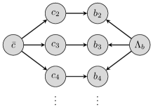
We proceed based on two independent assumptions: (1) the details of the chiral EFT description of low-energy QCD (e.g., renormalization scale and scheme) dictates a well-defined breakdown scale , and (2) a well-formulated EFT implementation will lead to natural expansion coefficients for observables. Although any given can be extracted from order-by-order calculations without any reference to a breakdown scale or naturalness, our assumptions imply that the value of manifests the interplay between the underlying and the natural required by Eq. (18). This relationship is represented graphically as a Bayesian network in Fig. 21.
We note that will not give any information on the expansion parameter, because it will not modify the convergence pattern. Because it is known that in chiral EFT, it too is omitted from our analysis.
In general, we want to use order-by-order calculations of several observables at several kinematic points to inform our estimate of . The full quantity of interest is therefore
| (19) |
where the given information is sets of coefficients labeled by : the set of kinematic parameters and observable from which the were calculated. Using Bayes theorem, we can express the posterior for as
| (20) |
We have assumed statistical independence of coefficients at different orders, but it is possible for to be correlated with . The coefficients can be correlated for multiple reasons: for a given observable, the kinematic parameters may be close to one another; two distinct observables could themselves be correlated; or a combination of both. Assuming statistical independence in , we can factor the likelihood in Eq. (20) into
| (21) |
Therefore, the posterior is given by
| (22) |
The denominator of Eq. (22) is simply a normalization constant and the prior can be chosen later on, leaving only to evaluate. For simplicity, we will refer to this as , noting that the likelihoods for all simply need to be multiplied together to get the final posterior pdf in Eq. (22).
To express in terms of the prior assumptions of naturalness, we first use marginalization Sivia and Skilling (2006) to introduce as auxiliary parameters the dimensionless coefficients [see Eq. (3)]:
| (23) |
Next, to express the prior pdf for the coefficients , we integrate in the naturalness parameter :
| (24) |
To simplify Eq. (24) we use independence as reflected in the causal relationship outlined in Fig. 21. Neither the s nor depend on if they are not mediated by . We adopt a prior of independence between the s as before. Thus
| (25) |
The s also only depend on their corresponding and , and are independent of one another. This means that
| (26) |
Therefore, Eq. (24) can be written as
| (27) |
The pdf for contingent on and is simply
| (28) |
which enables us to perform the integrations directly. Thus,
| (29) |
where we have used and have set from now on.
To evaluate Eq. (29), we must make choices for the priors, such as those from Table 1. Analytic expressions of Eq. (29) can be found for sets and , which we will consider here. It is reasonable to assume no prior knowledge of the scale of , i.e. allow and , because the scale can vary wildly with a changing . For set ,
| (30) |
The result for set is similar to Eq. (30), with the replacement , where . These likelihoods are maximized for values of where the individual s are about the same size.
The final step in specifying the posterior is to make a choice of . Here we employ a non-informative log-uniform prior as we did for :
| (31) |
which assumes we know only limits on the scale of . Then for set ,
| (32) |
where the functions on are implicit. A more probable region in is singled out in Eq. (32) by the interplay of the factors, which individually favor s that make the order-by-order s for each about the same size.
The lower limit in the prior of Eq. (31) requires comment: if is set less than the momentum scale corresponding to the lab energy where is calculated, the expansion parameter may be greater than one. If we have an EFT that converges according to our statistical model, for the relevant kinematic points should be excluded by Eq. (22). If it instead favors values of for which , this would signal an inconsistency between the truncation error model and the EFT as implemented.
As already noted, we assume that because of their separations in energy or angle, the chosen sets of kinematic parameters can be treated as independent from one another and their probability densities multiplied. We make a similar assumption for the observables themselves, i.e., the set labeled includes sets for each of the spin observables , , , and . The assumption of independence, particularly for observables at the same energy or angle, may be questioned. The exploration of methods to combine data from all kinematic parameters, such as through GPs Rasmussen and Williams (2006); Gelman et al. (2003); Jones et al. (1998), and assessments of observable independence, are currently in progress.
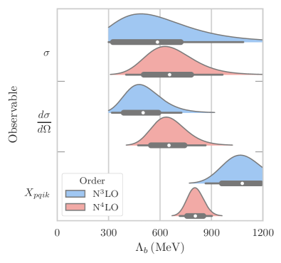
Given the above assumptions, we have applied Eq. (32) to various potentials, observable sets, and kinematic parameters; the resulting pdfs and DoB intervals, using the HPD prescription (see Sec. II), are presented in Figs. 22–26. In contrast to central credibility intervals, the HPD intervals ensure that massive extremes, such as the posterior for near its lower boundary in Fig. 22, are not necessarily excluded from our DoB intervals Kruschke (2011). The posteriors of Fig. 22 mirror the conclusions drawn from Fig. 16—both and predict MeV, while the set of spin observables, taken together, prefers MeV. The relatively small amount of data used from and do not allow for a very precise determination of .
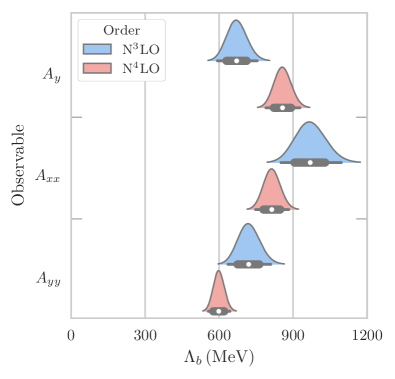
Figure 23 explores this result for spin observables by splitting out the posteriors for , , and separately. These posteriors can be qualitatively predicted from the order-by-order consistency plots for these observables given in Fig. 15. In general, the strength of the posterior at should be highly correlated with the pattern in the consistency plot at (e.g., do the points lie above or below the 45 degree line, which imply that and are more probable than , respectively). Similarly, the posterior at correlates with the pattern in the consistency plot at . For , this rule predicts that the posterior should have its strength concentrated well above 600 MeV, and that the posterior should be located to its left. For , the posterior should also be well above 600 MeV, but the posterior should be to its right. Finally, for , the consistency plots predict the posterior will be concentrated near 600 MeV (i.e., ), with the posterior shifted somewhat to the right. All of these expectations are realized in Fig. 23.
One may wonder to what extent the posteriors are stable under different choices of kinematic parameter sets. Figure 24 shows the posteriors as in Fig. 22, but with a different (lower) range of energies. Note that MeV is near the crossover region , where the interpretation of the expansion parameter is unclear. However, while there are systematic shifts, both sets of posteriors for and are consistent with the EKM value of MeV, with the ensemble spin observable posteriors favoring significantly higher values. In all cases there are wide posteriors at and more stability at . The only major shift in the median between these energy sets is for the cross section result. If we use larger sets of observables more closely spaced in both energy and angle (see Fig. 25), neglecting the possible danger from correlations, the posteriors become more narrow and more Gaussian, but are systematically in accord with Fig. 22.
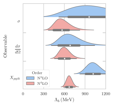
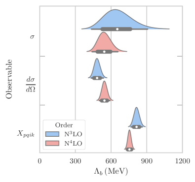
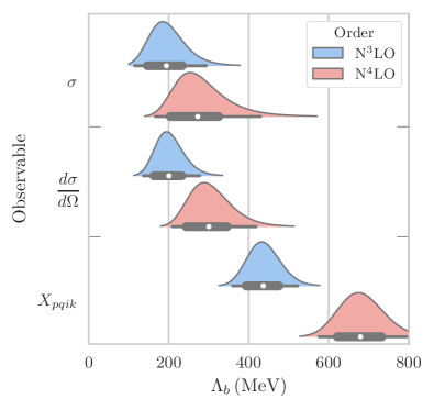
Figure 26 applies Eq. (32) to the fm EKM potential, for which EKM assumed that MeV. Most of the posteriors imply even smaller values of , except for the posterior for the spin observables, which is completely inconsistent. Following the earlier discussion of the lower limit on in the prior of Eq. (31), we see that the posteriors are not only indicating much lower values of , but they also weight areas where the expansion parameter . The cross section and differential cross section posteriors exhibit this behavior most, while the spin observable posteriors are maximized in regions where . The weighting of regions of the posterior is another indication that the EFT convergence for this regulator is not well-described by the statistical model.
VI Summary and outlook
In this work, we extend the analysis from Ref. Furnstahl et al. (2015b) that applies Bayesian statistics to the quantification of theoretical uncertainties in chiral EFT. Our approach makes testable predictions of DoB error bands based upon assumptions about the convergence pattern of EFT observables and an implementation of naturalness. In particular, we assume that the scaled observable coefficients defined in Eq. (1) are effectively random functions of natural size whose magnitude provides an estimate of the error incurred by truncating the EFT expansion.
We apply this model to a set of scattering observables predicted by the semi-local chiral EFT potentials of EKM Epelbaum et al. (2015b, a), who also proposed a non-statistical protocol for uncertainty quantification. The EKM error estimates in Epelbaum et al. (2015b) correspond most closely to the leading approximation of set (see Table 1). In particular their error bands at NkLO are DoB intervals Furnstahl et al. (2015b); i.e., they do not correspond to the same DoB at each order. Additionally, if the known next-order result does not lie in that DoB interval, EKM extends the interval to the next-order result. Therefore, at some orders it is possible to interpret the EKM intervals according to our truncation error model using set , but not always. To calculate consistent statistical DoBs at each order, we follow the statistical model outlined in Fig. 1, which assumes a natural convergence pattern for the EFT.
We begin by arguing that appropriate physical choices of scale in Eq. (1) are for and , while for any spin observable . We then validate a posteriori for these choices of the natural distribution of observable coefficients for the total cross section, differential cross section, and a selection of spin observables for the fm potential. The fm potential is also consistent with our statistical model. In contrast, the convergence patterns of the fm, 1.1 fm and 1.2 fm potentials become increasingly unsystematic, and hence they become less well described by this model. The expansion parameter for these softer potentials is dominated by regulator artifacts, which EKM account for by adopting a smaller value for . This reflects the effective cutoff in momentum space instead of the intrinsic breakdown scale of chiral EFT Furnstahl et al. (2015a). But the order-by-order convergence pattern is also modified as the long-range pion contributions at odd orders in are significantly shifted to short-range contributions at even orders. This is manifested in the coefficients extracted in Fig. 4 and the failed validation of DoBs in Figs. 19 and 20.
Our higher-order results are generally insensitive to the specific prior choice; we compare sets A and C in Figs. 12 and 13, and provide more examples in the Supplemental Material sup . The results for potentials with good convergence patterns (we focus on fm) can be summarized in terms of our progress on the questions raised in Sec. I:
-
1.
The observable coefficients of the total cross section vary smoothly with energy, typically changing sign once over the energy range from 0 to 350 MeV. There is no apparent order-by-order pattern at any given energy, which supports our model of a random distribution characterized by a size . The unnatural size of the coefficient at MeV was noted in Ref. Furnstahl et al. (2015b). At low energies, higher-ordered coefficients become more sensitive to the value assigned to the expansion parameter around the crossover region , for which we do not have a model. Hence we cannot make strong statements about the coefficient spectrum and its implication for naturalness in that energy region. We plan to test alternative schemes for in the crossover region and to validate the presence of the crossover in the s using a change-point analysis of the correlations modeled using a GP model Gramacy and Lee (2008); Rasmussen and Williams (2006); Jones et al. (1998); Gelman et al. (2003).
-
2.
The observable coefficients for both the differential cross section and the chosen spin observables vary smoothly in both and with characteristic sizes between about 1 and 5 for fm, which validates the assumption that naturalness propagates to these observables for this potential. The functional dependences show no obvious patterns, supporting the model of effectively random functions. As with the cross section, the interpretation of the coefficients is ambiguous for low energies.
-
3.
Because each is a smooth function when plotted against both and , the values of the observable coefficients at one value of the kinematic parameters are correlated within some neighborhood (a correlation length) of and . Through a rough estimation, we find that the correlation length in energy is about 80 MeV, while the correlation length in is approximately . These values were estimated visually here, but in the future we will determine them directly using a GP model for the s Rasmussen and Williams (2006); Jones et al. (1998); Gelman et al. (2003). This additional information will then be incorporated into our statistical model for truncation uncertainties.
-
4.
The checks in Sec. V.1 show that taking to be the same scale for both and is statistically consistent for the fm EKM potential. While the spin observable is also consistent with that same scale, the ensemble of spin observables are more consistent with a somewhat larger value. The fm EKM potential also shows promise, but extracting becomes questionable for fm and worse for larger . The posteriors for , shown in Sec. V.2 and the Supplemental Material sup , lead to the same conclusions—probable ranges of consistent with the values proposed by EKM can be extracted for and fm, identifying probable ranges for fm is questionable at best, and the other EKM potentials ( and fm) are not well described by our statistical model. Conclusions about are not warranted for the poorly behaving potentials.
An overall validation of our truncation error model as applied to the EKM potential with fm is provided in Fig. 27, which shows order-by-order consistency plots for observables compared with the NPWA data. These plots are made by modifying step 4. of the procedure laid out in Sec. V.1 to count a success when the actual NPWA result is within the DoB interval at that order (as opposed to comparison to the next-order calculation). In general, the error bands work as advertised, predicting the discrepancy with the NPWA data at the level to within expected fluctuations.
The general success of the model for chiral EFT truncation errors motivates additional applications, further development of the model (e.g., GP models), and its full integration into parameter estimation of LECs. We plan to apply our truncation error model to other chiral interactions that are available order-by-order, such as the recent potential of Entem, Machleidt, and Nosyk in Entem et al. (2017). Our error model and Bayesian model checking diagnostics can be applied not only for other chiral interactions but also for other EFTs in general. They also apply generically to any observable calculation that fulfills the expansion model in Eq. (1), including calculations in perturbation theory. A Bayesian-type Lepage plot analysis Lepage et al. (2002); Furnstahl et al. (2015a); Wesolowski et al. (2016) of the power-law behavior of residuals as a function of energy/momentum will complement the statistically motivated model checks of Sec. V. Now that we have a framework of testable assumptions for treating as a random variable in the posterior pdf calculations of Sec. V, that information can be used to marginalize over as an auxiliary parameter in truncation error estimates rather than using a fixed value. Work in these areas is in progress.
Acknowledgements.
We thank E. Epelbaum, H. Griesshammer, N. Klco, and D. Phillips for useful discussions. Useful feedback on the manuscript was provided by N. Klco and D. Phillips. This work was supported in part by the National Science Foundation under Grant Nos. PHY–1306250 and PHY–1614460 and the NUCLEI SciDAC Collaboration under Department of Energy Grant DE-SC0008533.Appendix A Derivations of Posteriors
Here we continue the analysis started in Sec. II by giving explicit forms of posteriors for various prior sets. The most non-informative case of set A follows if we take , and then take the limit at the end. We designate this as set , and the results for this set were first worked out in Cacciari and Houdeau (2011). If we further adopt the first-omitted-term approximation, designated , we have analytic expressions for Eq. (6),
| (33) |
and for from Eq. (4),
| (34) |
where
| (35) |
and is the number of relevant known coefficients—here, since and do not contribute to our analysis, but equations are given in a general form for the reader.
Relaxing the first-omitted-term approximation can pose a numerical challenge, since the integration volume grows quickly with increasing . Luckily, by following Ref. Coello Pérez and Papenbrock (2015), whose results we reproduce in Eqs. (36)–(38), Eq. (7) can be reduced to one integral for the hard-wall (hw) prior in sets A and B, and exactly evaluated for the Gaussian (G) prior in set C. For sets A and B,
| (36) |
which, for , becomes the atomic function Victor et al. (2009). For set C,
| (37) |
where
| (38) |
Equation (37) is easily evaluated for all ; we use unless otherwise specified, at which point the posteriors have converged numerically (see Ref. Furnstahl et al. (2015b)).
With Eq. (37), we can exactly evaluate Eq. (6) for set C in terms of special functions. By inserting the priors and making the variable substitution ,
| (39) |
where, of course,
| (40) |
Equation (39) can be evaluated in terms of the incomplete functions via
| (41) |
using the definition
| (42) |
Of all sets in Table 1, the posterior as given by set C, via Eq. (A), is the only one for which we have found a closed-form expression for all and ranges of .
Appendix B Details on NN observables
For convenience of the reader and because of the multitude of different conventions in the literature, we have gathered in this appendix the formulas used here in the calculation of NN observables MacGregor et al. (1960); Bystricky et al. (1978); La France and Winternitz (1980); Moravcsik et al. (1989); Stoks and de Swart (1990); Stoks et al. (1993b); Carlsson et al. (2016).
B.1 Kinematics

In the context of NN scattering, one particle (the beam), with kinetic energy , is incident on a stationary particle (the target). For scattering, the lab system (l.s.) is often taken to be the rest frame of the initial proton. In the center-of-momentum (c.m.) system, each particle has a relative momentum of . It is convenient to relate these quantities for each NN experiment:
| (45) | ||||
| (46) | ||||
| (47) |
where relativistic kinematics is used Epelbaum et al. (2015b). Unless otherwise stated, is the c.m. polar scattering angle while denotes the azimuthal scattering angle. For our purposes, can be set to zero because all observables can be defined relative to the scattering plane.
The spin states of the initial and final states can be expressed in the uncoupled basis and , respectively, where we have suppressed . We can also use the coupled singlet-triplet basis, where and .
B.2 Observables
Because nucleons have nonzero intrinsic spin, observables in general are dependent not only on kinematic variables (), but also on the relative orientation of the particles’ spin. A generic spin observable can be written as
| (48) |
where is the (unpolarized) differential cross section, is the spin-scattering matrix and . The subscripts , , , and refer to the polarization directions of the scattered, recoil, beam, and target particles, respectively. If a final-state subscript is zero, its polarization is not analyzed. If a initial-state subscript is zero, the corresponding particle was unpolarized.
When an observable is considered in the c.m. system, the polarization of each particle is often decomposed in a common basis using the unit vectors , , defined as
| (49) | ||||
| (50) | ||||
| (51) |
and shown in Fig. 28. Here we consider pure experiments, where the spin projections are solely along the basis vectors. Hence, for a c.m. observable, the subscripts , , , and are some combination of , , , and 0.
It is often convenient to express spin observables in the l.s., where the scattered and recoil particles deflect at angles and , respectively. Lab system observables often use three sets of bases to define spin observables, defined by the beam, scattered, and recoil particle directions. The beam (scattered, recoil) frame aligns (, ) with the lab particle momentum and defines () to be normal to the scattering plane, which leaves (, ) in the scattering plane such that (, ). The initial-state subscripts and are then chosen to be , , , or . Similarly, the scattered-state subscript is , , or , and the recoil-state subscript is , , or .
One added complication of calculating l.s. observables involves accounting for the relativistic spin rotation angles
| (52) | ||||
| (53) |
which rotate the primed and double primed vectors about , respectively. It is the rotated vectors, denoted with subscripts and , that correspond to the l.s. subscripts for the scattered and recoil particles. In the nonrelativistic case, and , which implies that
| (54) | ||||
| (55) |
This too is illustrated in Fig. 28. Whether an observable is defined in the c.m. system or the l.s. should be clear from the chosen subscripts. All of the observables considered here use the l.s. notation.
Notational inconsistencies abound in the literature. While the subscripts of Eq. (48) completely determine a given spin observable, often the is changed to match historical usage. Other times, the subscript notation is abandoned completely for a nondescript letter. Table 2 attempts to reconcile some differences by matching a common name with Eq. (48) and other popular notations found in literature.
| Name | Others | |
|---|---|---|
| Differential Cross Section | , | |
| Vector Analyzing Power | , | |
| Polarization Transfer | ||
| Spin Correlation Parameters | ||
The spin-scattering matrix is the part of the scattering matrix that is due to interactions. In our convention, they are related via . To evaluate , it is useful to write it in singlet-triplet space, and then make a partial-wave expansion
| (56) |
where and , the second line contains two Wigner symbols, and is the total angular momentum decomposed into orbital and intrinsic angular momentum. The nuclear potential conserves the total angular momentum , but generally mixes the states of and . Equation (B.2) becomes useful only if a small number of waves are needed to accurately determine .
When a partial wave state is uncoupled, such as when , then can be parameterized by a real phase such that . For , is 4-dimensional in angular momentum space and can be written compactly using the triplet submatrix and the singlet-triplet submatrix via
| (57) |
The triplet submatrix can be parameterized by introducing another real parameter, the mixing angle . Using the common notation that subscripts and refer to and , respectively, then
| (58) |
and similarly
| (59) |
In the present work, for all , leaving the singlet-triplet submatrix uncoupled and thus .
Equations (58) and (59) employ the “Stapp”- or “bar”-phase shift parameterization. Another parameterization, with phases and mixing angle denoted here by and , was made by Blatt and Biedenharn Blatt and Biedenharn (1952):
| (60) |
where
| (61) |
The Blatt eigenphases are related to the Stapp phases via
| (62) | ||||
| (63) | ||||
| (64) |
Given the partial-wave-projected potential , it is convenient and numerically accurate to solve the Lippmann-Schwinger (LS) equation with standing wave boundary conditions,
| (65) |
for the partial-wave-projected matrix (known as the -matrix in other contexts). In the present work we use Gaussian quadrature to reduce the LS equation to a system of linear equations, from which is extracted Landau (1996). Having solved Eq. (B.2), the on-shell matrix then leads directly to the phases and mixing angle. For the uncoupled channels,
| (66) |
For coupled channels, is 2-dimensional. The Blatt-Biedenharn phases and are extractable via
| (67) | ||||
| (68) | ||||
| (69) |
which can then be converted to the Stapp convention using Eqs. (62)–(64).
References
- Barrett et al. (2013) B. R. Barrett, P. Navratil, and J. P. Vary, Prog. Part. Nucl. Phys. 69, 131 (2013).
- Hagen et al. (2014) G. Hagen, T. Papenbrock, M. Hjorth-Jensen, and D. J. Dean, Rept. Prog. Phys. 77, 096302 (2014), arXiv:1312.7872 [nucl-th] .
- Carlson et al. (2015) J. Carlson, S. Gandolfi, F. Pederiva, S. C. Pieper, R. Schiavilla, K. E. Schmidt, and R. B. Wiringa, Rev. Mod. Phys. 87, 1067 (2015), arXiv:1412.3081 [nucl-th] .
- Hergert et al. (2016) H. Hergert, S. K. Bogner, J. G. Lietz, T. D. Morris, S. Novario, N. M. Parzuchowski, and F. Yuan, (2016), arXiv:1612.08315 [nucl-th] .
- Barbieri and Carbone (2016) C. Barbieri and A. Carbone, (2016), arXiv:1611.03923 [nucl-th] .
- Lee (2016) D. Lee, (2016), arXiv:1609.00421 [nucl-th] .
- Epelbaum et al. (2009) E. Epelbaum, H.-W. Hammer, and U.-G. Meissner, Rev. Mod. Phys. 81, 1773 (2009), arXiv:0811.1338 [nucl-th] .
- Machleidt and Entem (2011) R. Machleidt and D. R. Entem, Phys. Rept. 503, 1 (2011), arXiv:1105.2919 [nucl-th] .
- Gezerlis et al. (2014) A. Gezerlis, I. Tews, E. Epelbaum, M. Freunek, S. Gandolfi, K. Hebeler, A. Nogga, and A. Schwenk, Phys. Rev. C90, 054323 (2014), arXiv:1406.0454 [nucl-th] .
- Epelbaum et al. (2015a) E. Epelbaum, H. Krebs, and U. G. Meißner, Phys. Rev. Lett. 115, 122301 (2015a), arXiv:1412.4623 [nucl-th] .
- Piarulli et al. (2015) M. Piarulli, L. Girlanda, R. Schiavilla, R. Navarro Pérez, J. E. Amaro, and E. Ruiz Arriola, Phys. Rev. C91, 024003 (2015), arXiv:1412.6446 [nucl-th] .
- Entem et al. (2017) D. R. Entem, R. Machleidt, and Y. Nosyk, (2017), arXiv:1703.05454 [nucl-th] .
- Dobaczewski et al. (2014) J. Dobaczewski, W. Nazarewicz, and P.-G. Reinhard, J. Phys. G 41, 074001 (2014), arXiv:1402.4657 [nucl-th] .
- Ireland and Nazarewicz (2015) D. G. Ireland and W. Nazarewicz, Journal of Physics G: Nuclear and Particle Physics 42, 030301 (2015).
- Carlsson et al. (2016) B. D. Carlsson, A. Ekström, C. Forssén, D. F. Strömberg, G. R. Jansen, O. Lilja, M. Lindby, B. A. Mattsson, and K. A. Wendt, Phys. Rev. X6, 011019 (2016), arXiv:1506.02466 [nucl-th] .
- Furnstahl et al. (2015a) R. J. Furnstahl, D. R. Phillips, and S. Wesolowski, J. Phys. G42, 034028 (2015a), arXiv:1407.0657 [nucl-th] .
- Furnstahl et al. (2015b) R. J. Furnstahl, N. Klco, D. R. Phillips, and S. Wesolowski, Phys. Rev. C 92, 024005 (2015b), arXiv:1506.01343 [nucl-th] .
- Cacciari and Houdeau (2011) M. Cacciari and N. Houdeau, JHEP 1109, 039 (2011), arXiv:1105.5152 [hep-ph] .
- Bagnaschi and Jenniches (2014) E. Bagnaschi and L. Jenniches, in Proceedings, 49th Rencontres de Moriond on QCD and High Energy Interactions: La Thuile, Italy, March 22-29, 2014 (2014) pp. 301–308.
- Epelbaum et al. (2015b) E. Epelbaum, H. Krebs, and U. G. Meißner, Eur. Phys. J. A 51, 53 (2015b), arXiv:1412.0142 [nucl-th] .
- Gelman et al. (2013) A. Gelman, J. Carlin, H. Stern, D. Dunson, A. Vehtari, and D. Rubin, Bayesian Data Analysis, Third Edition, Chapman & Hall/CRC Texts in Statistical Science (Taylor & Francis, 2013).
- (22) See Supplemental Material at [URL will be inserted by publisher] for extra figures and data that helped inform our conclusions.
- Kruschke (2011) J. K. Kruschke, Doing Bayesian data analysis: a tutorial with R and BUGS (Academic Press, Burlington, MA, 2011).
- Liu et al. (2015) Y. Liu, A. Gelman, and T. Zheng, Statistics and Computing 25, 809 (2015).
- Ben-Gal (2007) I. Ben-Gal, Encyclopedia of statistics in quality and reliability (2007).
- Puga et al. (2015) J. L. L. Puga, M. Krzywinski, and N. Altman, Nature methods 12, 799 (2015).
- Gull (1998) S. F. Gull, in Maximum entropy and Bayesian methods in science and engineering, vol. 1, edited by G. J. Erickson and C. R. Smith (Kluwer, Dordrecht, 1998).
- Sivia and Skilling (2006) D. Sivia and J. Skilling, Data Analysis: A Bayesian Tutorial (Oxford University Press, 2006).
- Schindler and Phillips (2009) M. R. Schindler and D. R. Phillips, Annals Phys. 324, 682 (2009), arXiv:0808.3643 [hep-ph] .
- Jeffreys (1939) H. Jeffreys, Theory of Probability (Clarendon Press, 1939).
- Bagnaschi et al. (2015) E. Bagnaschi, M. Cacciari, A. Guffanti, and L. Jenniches, JHEP 02, 133 (2015), arXiv:1409.5036 [hep-ph] .
- Wesolowski and Furnstahl (2017) S. Wesolowski and R. J. Furnstahl, (2017), in preparation.
- Stoks et al. (1993a) V. G. J. Stoks, R. A. M. Klomp, M. C. M. Rentmeester, and J. J. de Swart, Phys. Rev. C 48, 792 (1993a).
- Rasmussen and Williams (2006) C. Rasmussen and C. Williams, Gaussian Processes for Machine Learning, Adaptative computation and machine learning series (University Press Group Limited, 2006).
- Gelman et al. (2003) A. Gelman, J. B. Carlin, H. S. Stern, and D. B. Rubin, Bayesian Data Analysis (Chapman and Hall/CRC, 2003).
- Jones et al. (1998) D. R. Jones, M. Schonlau, and W. J. Welch, Journal of Global Optimization 13, 455 (1998).
- Gramacy and Lee (2008) R. B. Gramacy and H. K. H. Lee, Journal of the American Statistical Association 103, 1119 (2008).
- Lepage et al. (2002) G. Lepage, B. Clark, C. Davies, K. Hornbostel, P. Mackenzie, et al., Nucl. Phys. Proc. Suppl. 106, 12 (2002), arXiv:hep-lat/0110175 [hep-lat] .
- Wesolowski et al. (2016) S. Wesolowski, N. Klco, R. J. Furnstahl, D. R. Phillips, and A. Thapaliya, J. Phys. G43, 074001 (2016), arXiv:1511.03618 [nucl-th] .
- Coello Pérez and Papenbrock (2015) E. A. Coello Pérez and T. Papenbrock, Phys. Rev. C92, 064309 (2015), arXiv:1510.02401 [nucl-th] .
- Victor et al. (2009) K. Victor, P.-M. Hector, and P. Volodymyr, Adaptive digital processing of multidimensional signals with applications (2009).
- MacGregor et al. (1960) M. H. MacGregor, M. J. Moravcsik, and M. J. Stapp, Annual Review of Nuclear Science 10, 291 (1960), http://dx.doi.org/10.1146/annurev.ns.10.120160.001451 .
- Bystricky et al. (1978) J. Bystricky, F. Lehar, and P. Winternitz, J. Phys.(France) 39, 1 (1978).
- La France and Winternitz (1980) P. La France and P. Winternitz, Journal de Physique 41, 1391 (1980).
- Moravcsik et al. (1989) M. J. Moravcsik, J. Pauschenwein, and G. R. Goldstein, Journal de Physique 50, 1167 (1989).
- Stoks and de Swart (1990) V. G. J. Stoks and J. J. de Swart, Phys. Rev. C42, 1235 (1990).
- Stoks et al. (1993b) V. G. J. Stoks, R. A. M. Klomp, M. C. M. Rentmeester, and J. J. de Swart, Phys. Rev. C48, 792 (1993b).
- Blatt and Biedenharn (1952) J. M. Blatt and L. C. Biedenharn, Phys. Rev. 86, 399 (1952).
- Landau (1996) R. H. Landau, Quantum Mechanics II, 2nd ed. (John Wiley & Sons, Inc., New York, 1996).