Interpretable Explanations of Black Boxes by Meaningful Perturbation
Abstract
As machine learning algorithms are increasingly applied to high impact yet high risk tasks, such as medical diagnosis or autonomous driving, it is critical that researchers can explain how such algorithms arrived at their predictions. In recent years, a number of image saliency methods have been developed to summarize where highly complex neural networks “look” in an image for evidence for their predictions. However, these techniques are limited by their heuristic nature and architectural constraints.
In this paper, we make two main contributions: First, we propose a general framework for learning different kinds of explanations for any black box algorithm. Second, we specialise the framework to find the part of an image most responsible for a classifier decision. Unlike previous works, our method is model-agnostic and testable because it is grounded in explicit and interpretable image perturbations.
1 Introduction
Given the powerful but often opaque nature of modern black box predictors such as deep neural networks [4, 5], there is a considerable interest in explaining and understanding predictors a-posteriori, after they have been learned. This remains largely an open problem. One reason is that we lack a formal understanding of what it means to explain a classifier. Most of the existing approaches [19, 16, 8, 7, 9, 19], etc., often produce intuitive visualizations; however, since such visualizations are primarily heuristic, their meaning remains unclear.
In this paper, we revisit the concept of “explanation” at a formal level, with the goal of developing principles and methods to explain any black box function , e.g. a neural network object classifier. Since such a function is learned automatically from data, we would like to understand what has learned to do and how it does it. Answering the “what” question means determining the properties of the map. The “how” question investigates the internal mechanisms that allow the map to achieve these properties. We focus mainly on the “what” question and argue that it can be answered by providing interpretable rules that describe the input-output relationship captured by . For example, one rule could be that is rotation invariant, in the sense that “ whenever images and are related by a rotation”.

In this paper, we make several contributions. First, we propose the general framework of explanations as meta-predictors (sec. 2), extending [18]’s work. Second, we identify several pitfalls in designing automatic explanation systems. We show in particular that neural network artifacts are a major attractor for explanations. While artifacts are informative since they explain part of the network behavior, characterizing other properties of the network requires careful calibration of the generality and interpretability of explanations. Third, we reinterpret network saliency in our framework. We show that this provides a natural generalization of the gradient-based saliency technique of [15] by integrating information over several rounds of backpropagation in order to learn an explanation. We also compare this technique to other methods [15, 16, 20, 14, 19] in terms of their meaning and obtained results.
2 Related work
Our work builds on [15]’s gradient-based method, which backpropagates the gradient for a class label to the image layer. Other backpropagation methods include DeConvNet [19] and Guided Backprop [16, 8], which builds off of DeConvNet [19] and [15]’s gradient method to produce sharper visualizations.
Another set of techniques incorporate network activations into their visualizations: Class Activation Mapping (CAM) [22] and its relaxed generalization Grad-CAM [14] visualize the linear combination of a late layer’s activations and class-specific weights (or gradients for [14]), while Layer-Wise Relevance Propagation (LRP) [1] and Excitation Backprop [20] backpropagate an class-specific error signal though a network while multiplying it with each convolutional layer’s activations.
With the exception of [15]’s gradient method, the above techniques introduce different backpropagation heuristics, which results in aesthetically pleasing but heuristic notions of image saliency. They also are not model-agnostic, with most being limited to neural networks (all except [15, 1]) and many requiring architectural modifications [19, 16, 8, 22] and/or access to intermediate layers [22, 14, 1, 20].
A few techniques examine the relationship between inputs and outputs by editing an input image and observing its effect on the output. These include greedily graying out segments of an image until it is misclassified [21] and visualizing the classification score drop when an image is occluded at fixed regions [19]. However, these techniques are limited by their approximate nature; we introduce a differentiable method that allows for the effect of the joint inclusion/exclusion of different image regions to be considered.
Our research also builds on the work of [18, 12, 2]. The idea of explanations as predictors is inspired by the work of [18], which we generalize to new types of explanations, from classification to invariance.
The Local Intepretable Model-Agnostic Explanation (LIME) framework [12] is relevant to our local explanation paradigm and saliency method (sections 3.2, 4) in that both use an function’s output with respect to inputs from a neighborhood around an input that are generated by perturbing the image. However, their method takes much longer to converge ( vs. our iterations) and produces a coarse heatmap defined by fixed super-pixels.
Similar to how our paradigm aims to learn an image perturbation mask that minimizes a class score, feedback networks [2] learn gating masks after every ReLU in a network to maximize a class score. However, our masks are plainly interpretable as they directly edit the image while [2]’s ReLU gates are not and can not be directly used as a visual explanation; furthermore, their method requires architectural modification and may yield different results for different networks, while ours is model-agnostic.


3 Explaining black boxes with meta-learning
A black box is a map from an input space to an output space , typically obtained from an opaque learning process. To make the discussion more concrete, consider as input color images where is a discrete domain. The output can be a boolean telling whether the image contains an object of a certain type (e.g. a robin), the probability of such an event, or some other interpretation of the image content.
3.1 Explanations as meta-predictors
An explanation is a rule that predicts the response of a black box to certain inputs. For example, we can explain a behavior of a robin classifier by the rule , where is the subset of all the robin images. Since is imperfect, any such rule applies only approximately. We can measure the faithfulness of the explanation as its expected prediction error: , where is the indicator function of event . Note that implicitly requires a distribution over possible images . Note also that is simply the expected prediction error of the classifier. Unless we did not know that was trained as a robin classifier, is not very insightful, but it is interpretable since is.
Explanations can also make relative statements about black box outcomes. For example, a black box , could be rotation invariant: , where means that and are related by a rotation. Just like before, we can measure the faithfulness of this explanation as .111For rotation invariance we condition on because the probability of independently sampling rotated and is zero, so that, without conditioning, would be true with probability 1. This rule is interpretable because the relation is.
Learning explanations.
A significant advantage of formulating explanations as meta predictors is that their faithfulness can be measured as prediction accuracy. Furthermore, machine learning algorithms can be used to discover explanations automatically, by finding explanatory rules that apply to a certain classifier out of a large pool of possible rules .
In particular, finding the most accurate explanation is similar to a traditional learning problem and can be formulated computationally as a regularized empirical risk minimization such as:
| (1) |
Here, the regularizer has two goals: to allow the explanation to generalize beyond the samples considered in the optimization and to pick an explanation which is simple and thus, hopefully, more interpretable.
Maximally informative explanations.
Simplicity and interpretability are often not sufficient to find good explanations and must be paired with informativeness. Consider the following variant of rule : , where means that and are related by a rotation of an angle . Explanations for larger angles imply the ones for smaller ones, with being trivially satisfied. The regularizer can then be used to select a maximal angle and thus find an explanation that is as informative as possible.222Naively, strict invariance for any implies invariance to arbitrary rotations as small rotations compose into larger ones. However, the formulation can still be used to describe rotation insensitivity (when varies slowly with rotation), or ’s meaning can be changed to indicate rotation w.r.t. a canonical “upright” direction for a certain object classes, etc.
3.2 Local explanations
A local explanation is a rule that predicts the response of in a neighborhood of a certain point . If is smooth at , it is natural to construct by using the first-order Taylor expansion of :
| (2) |
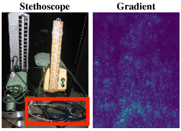
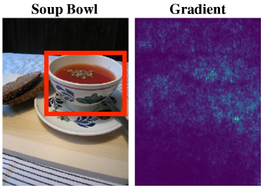
This formulation provides an interpretation of [15]’s saliency maps, which visualize the gradient as an indication of salient image regions. They argue that large values of the gradient identify pixels that strongly affect the network output. However, an issue is that this interpretation breaks for a linear classifier: If , is independent of the image and hence cannot be interpreted as saliency.
The reason for this failure is that eq. 2 studies the variation of for arbitrary displacements from and, for a linear classifier, the change is the same regardless of the starting point . For a non-linear black box such as a neural network, this problem is reduced but not eliminated, and can explain why the saliency map is rather diffuse, with strong responses even where no obvious information can be found in the image (fig. 3).
We argue that the meaning of explanations depends in large part on the meaning of varying the input to the black box. For example, explanations in sec. 3.1 are based on letting vary in image category or in rotation. For saliency, one is interested in finding image regions that impact ’s output. Thus, it is natural to consider perturbations obtained by deleting subregions of . If we model deletion by multiplying point-wise by a mask , this amounts to studying the function 333 is the Hadamard or element-wise product of vectors.. The Taylor expansion of at is For a linear classifier , this results in the saliency , which is large for pixels for which and are large simultaneously. We refine this idea for non-linear classifiers in the next section.
4 Saliency revisited


4.1 Meaningful image perturbations
In order to define an explanatory rule for a black box , one must start by specifying which variations of the input will be used to study . The aim of saliency is to identify which regions of an image are used by the black box to produce the output value . We can do so by observing how the value of changes as is obtained “deleting” different regions of . For example, if denotes a robin image, we expect that as well unless the choice of deletes the robin from the image. Given that is a perturbation of , this is a local explanation (sec. 3.2) and we expect the explanation to characterize the relationship between and .
While conceptually simple, there are several problems with this idea. The first one is to specify what it means “delete” information. As discussed in detail in sec. 4.3, we are generally interested in simulating naturalistic or plausible imaging effect, leading to more meaningful perturbations and hence explanations. Since we do not have access to the image generation process, we consider three obvious proxies: replacing the region with a constant value, injecting noise, and blurring the image (fig. 4).
Formally, let be a mask, associating each pixel with a scalar value . Then the perturbation operator is defined as
where is an average color, are i.i.d. Gaussian noise samples for each pixel and is the maximum isotropic standard deviation of the Gaussian blur kernel (we use , which yields a significantly blurred image).
4.2 Deletion and preservation
Given an image , our goal is to summarize compactly the effect of deleting image regions in order to explain the behavior of the black box. One approach to this problem is to find deletion regions that are maximally informative.
In order to simplify the discussion, in the rest of the paper we consider black boxes that generate a vector of scores for different hypotheses about the content of the image (e.g. as a softmax probability layer in a neural network). Then, we consider a “deletion game” where the goal is to find the smallest deletion mask that causes the score to drop significantly, where is the target class. Finding can be formulated as the following learning problem:
| (3) |
where encourages most of the mask to be turned off (hence deleting a small subset of ). In this manner, we can find a highly informative region for the network.
One can also play an symmetric “preservation game”, where the goal is to find the smallest subset of the image that must be retained to preserve the score : . The main difference is that the deletion game removes enough evidence to prevent the network from recognizing the object in the image, whereas the preservation game finds a minimal subset of sufficient evidence.
Iterated gradients.
Both optimization problems are solved by using a local search by means of gradient descent methods. In this manner, our method extracts information from the black box by computing its gradient, similar to the approach of [15]. However, it differs in that it extracts this information progressively, over several gradient evaluations, accumulating increasingly more information over time.
4.3 Dealing with artifacts
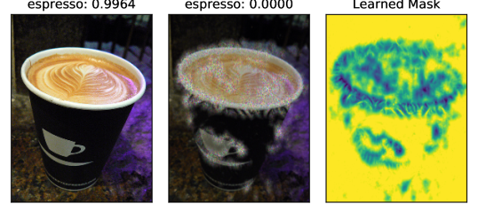

By committing to finding a single representative perturbation, our approach incurs the risk of triggering artifacts of the black box. Neural networks, in particular, are known to be affected by surprising artifacts [5, 10, 7]; these works demonstrate that it is possible to find particular inputs that can drive the neural network to generate nonsensical or unexpected outputs. This is not entirely surprising since neural networks are trained discriminatively on natural image statistics. While not all artifacts look “unnatural”, nevertheless they form a subset of images that is sampled with negligible probability when the network is operated normally.
Although the existence and characterization of artifacts is an interesting problem per se, we wish to characterize the behavior of black boxes under normal operating conditions. Unfortunately, as illustrated in fig. 5, objectives such as eq. 3 are strongly attracted by such artifacts, and naively learn subtly-structured deletion masks that trigger them. This is particularly true for the noise and constant perturbations as they can more easily than blur create artifacts using sharp color contrasts (fig. 5, bottom row).
We suggests two approaches to avoid such artifacts in generating explanations. The first one is that powerful explanations should, just like any predictor, generalize as much as possible. For the deletion game, this means not relying on the details of a singly-learned mask . Hence, we reformulate the problem to apply the mask stochastically, up to small random jitter.
Second, we argue that masks co-adapted with network artifacts are not representative of natural perturbations. As noted before, the meaning of an explanation depends on the meaning of the changes applied to the input ; to obtain a mask more representative of natural perturbations we can encourage it to have a simple, regular structure which cannot be co-adapted to artifacts. We do so by regularizing in total-variation (TV) norm and upsampling it from a low resolution version.
With these two modifications, eq. 3 becomes:
| (4) |
where . is the upsampled mask and is a 2D Gaussian kernel. Equation 4 can be optimized using stochastic gradient descent.
Implementation details.
Unless otherwise specified, the visualizations shown were generated using Adam [3] to minimize GoogLeNet’s [17] softmax probability of the target class by using the blur perturbation with the following parameters: learning rate iterations, upsampling a mask ( for GoogLeNet) by a factor of , blurring the upsampled mask with , and jittering the mask by drawing an integer from the discrete uniform distribution on where . We initialize the mask as the smallest centered circular mask that suppresses the score of the original image by when compared to that of the fully perturbed image, i.e. a fully blurred image.
5 Experiments
5.1 Interpretability


An advantage of the proposed framework is that the generated visualizations are clearly interpretable. For example, the deletion game produces a minimal mask that prevents the network from recognizing the object.
When compared to other techniques (fig. 2), this method can pinpoint the reason why a certain object is recognized without highlighting non-essential evidence. This can be noted in fig. 2 for the CD player (row 7) where other visualizations also emphasize the neighboring speakers, and similarly for the cliff (row 3), the street sign (row 4), and the sunglasses (row 8). Sometimes this shows that only a part of an object is essential: the face of the Pekenese dog (row 2), the upper half of the truck (row 6), and the spoon on the chocolate sauce plate (row 1) are all found to be minimally sufficient parts.
While contrastive excitation backprop generated heatmaps that were most similar to our masks, our method introduces a quantitative criterion (i.e., maximally suppressing a target class score), and its verifiable nature (i.e., direct edits to an image), allows us to compare differing proposed saliency explanations and demonstrate that our learned masks are better on this metric. In fig. 6, row 2, we show that applying a bounded perturbation informed by our learned mask significantly suppresses the truck softmax score, whereas a boxed perturbation on the truck’s back bumper, which is highlighted by contrastive excitation backprop in fig. 2, row 6, actually increases the score from to .
The principled interpretability of our method also allows us to identify instances when an algorithm may have learned the wrong association. In the case of the chocolate sauce in fig. 6, row 1, it is surprising that the spoon is highlighted by our learned mask, as one might expect the sauce-filled jar to be more salient. However, manually perturbing the image reveals that indeed the spoon is more suppressive than the jar. One explanation is that the ImageNet “chocolate sauce” images contain more spoons than jars, which appears to be true upon examining some images. More generally, our method allows us to diagnose highly-predictive yet non-intuitive and possibly misleading correlations by identified machine learning algorithms in the data.
5.2 Deletion region representativeness
To test that our learned masks are generalizable and robust against artifacts, we simplify our masks by further blurring them and then slicing them into binary masks by thresholding the smoothed masks by (fig. 7, top; tends to cover the salient part identified by the learned mask). We then use these simplified masks to edit a set of 5,000 ImageNet images with constant, noise, and blur perturbations. Using GoogLeNet [17], we compute normalized softmax probabilities444, where are the masked, original, and fully blurred images’ scores (fig. 7, bottom). The fact that these simplified masks quickly suppress scores as increases for all three perturbations gives confidence that the learned masks are identifying the right regions to perturb and are generalizable to a set of extracted masks and other perturbations that they were not trained on.


5.3 Minimality of deletions
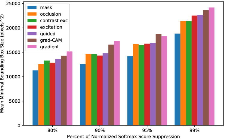
In this experiments we assess the ability of our method to correctly identify a minimal region that suppresses the object. Given the output saliency map, we normalize its intensities to lie in the range , threshold it with , and fit the tightest bounding box around the resulting heatmap. We then blur the image in the box and compute the normalized4 target softmax probability from GoogLeNet [17] of the partially blurred image.
From these bounding boxes and normalized scores, for a given amount of score suppression, we find the smallest bounding box that achieves that amount of suppression. Figure 8 shows that, on average, our method yields the smallest minimal bounding boxes when considering suppressive effects of . These results show that our method finds a small salient area that strongly impacts the network.
5.4 Testing hypotheses: animal part saliency
From qualitatively examining learned masks for different animal images, we noticed that faces appeared to be more salient than appendages like feet. Because we produce dense heatmaps, we can test this hypothesis. From an annotated subset of the ImageNet dataset that identifies the keypoint locations of non-occluded eyes and feet of vertebrate animals [11], we select images from classes that have at least 10 images which each contain at least one eye and foot annotation, resulting in a set of 3558 images from 76 animal classes (fig. 9). For every keypoint, we calculate the average heatmap intensity of a window around the keypoint. For all 76 classes, the mean average intensity of eyes were lower and thus more salient than that of feet (see supplementary materials for class-specific results).

5.5 Adversarial defense
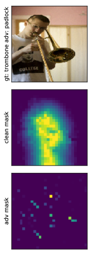
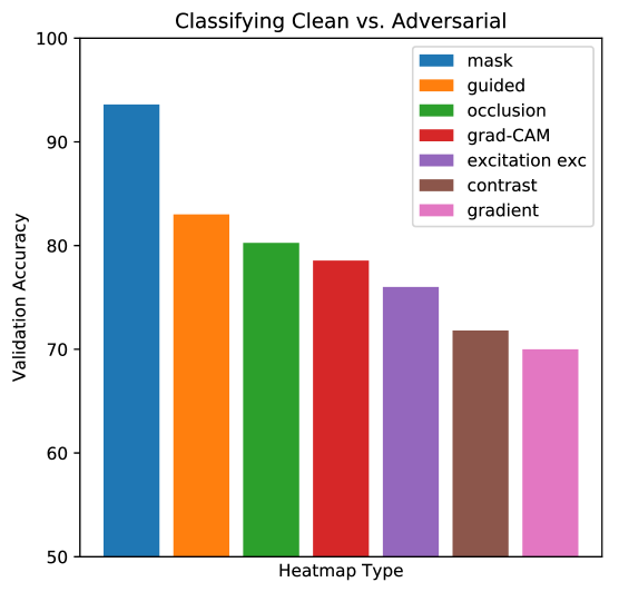
Adversarial examples [5] are often generated using a complementary optimization procedure to our method that learns a imperceptible pattern of noise which causes an image to be misclassified when added to it. Using our re-implementation of the highly effective one-step iterative method () [5] to generate adversarial examples, our method yielded visually distinct, abnormal masks compared to those produced on natural images (fig. 10, left). We train an Alexnet [4] classifier (learning rate , weight decay , and momentum ) to distinguish between clean and adversarial images by using a given heatmap visualization with respect to the top predicted class on the clean and adversarial images (fig. 10, right); our method greatly outperforms the other methods and achieves a discriminating accuracy of .
Lastly, when our learned masks are applied back to their corresponding adversarial images, they not only minimize the adversarial label but often allow the original, predicted label from the clean image to rise back as the top predicted class. Our method recovers the original label predicted on the clean image 40.64% of time and the ground truth label 37.32% (). Moreover, 100% of the time the original, predicted label was recovered as one of top-5 predicted labels in the “mask+adversarial” setting. To our knowledge, this is the first work that is able to recover originally predicted labels without any modification to the training set-up and/or network architecture.
5.6 Localization and pointing
Saliency methods are often assessed in terms of weakly-supervised localization and a pointing game [20], which tests how discriminative a heatmap method is by calculating the precision with which a heatmap’s maximum point lies on an instance of a given object class, for more harder datasets like COCO [6]. Because the deletion game is meant to discover minimal salient part and/or spurious correlation, we do not expect it to be particularly competitive on localization and pointing but tested them for completeness.
For localization, similar to [20, 2], we predict a bounding box for the most dominant object in each of 50k ImageNet [13] validation images and employ three simple thresholding methods for fitting bounding boxes. First, for value thresholding, we normalize heatmaps to be in the range of and then threshold them by their value with . Second, for energy thresholding [2], we threshold heatmaps by the percentage of energy their most salient subset covered with . Finally, with mean thresholding [20], we threshold a heatmap by , where is the mean intensity of the heatmap and . For each thresholding method, we search for the optimal value on a heldout set. Localization error was calculated as the IOU with a threshold of .
Table 1 confirms that our method performs reasonably and shows that the three thresholding techniques affect each method differently. Non-contrastive, excitation backprop [20] performs best when using energy and mean thresholding; however, our method performs best with value thresholding and is competitive when using the other methods: It beats gradient [15] and guided backprop [16] when using energy thresholding; beats LRP [1], CAM [22], and contrastive excitation backprop [20] when using mean thresholding (recall from fig. 2 that the contrastive method is visually most similar to mask); and out-performs Grad-CAM [14] and occlusion [19] for all thresholding methods.
| Val-* | Err (%) | Ene-* | Err | Mea-* | Err | |
| Grad [15] | 0.25 | 46.0 | 0.10 | 43.9 | 5.0 | 41.7§ |
| Guid [16, 8] | 0.05 | 50.2 | 0.30 | 47.0 | 4.5 | 42.0§ |
| Exc [20] | 0.15 | 46.1 | 0.60 | 38.7 | 1.5 | 39.0§ |
| C Exc [20] | — | — | — | — | 0.0 | 57.0† |
| Feed [2] | — | — | 0.95 | 38.8† | — | — |
| LRP [1] | — | — | — | — | 1.0 | 57.8† |
| CAM [22] | — | — | — | — | 1.0 | 48.1† |
| Grad-CAM [14] | 0.30 | 48.1 | 0.70 | 48.0 | 1.0 | 47.5 |
| Occlusion [19] | 0.30 | 51.2 | 0.55 | 49.4 | 1.0 | 48.6 |
| Mask‡ | 0.10 | 44.0 | 0.95 | 43.1 | 0.5 | 43.2 |
For pointing, table 2 shows that our method outperforms the center baseline, gradient, and guided backprop methods and beats Grad-CAM on the set of difficult images (images for which 1) the total area of the target category is less than of the image and 2) there are at least two different object classes). We noticed qualitatively that our method did not produce salient heatmaps when objects were very small. This is due to L1 and TV regularization, which yield well-formed masks for easily visible objects. We test two variants of occlusion [19], blur and variable occlusion, to interrogate if 1) the blur perturbation with smoothed masks is most effective, and 2) using the smallest, highly suppressive mask is sufficient (Occ§ and V-Occ in table 2 respectively). Blur occlusion outperforms all methods except contrast excitation backprop while variable while variable occlusion outperforms all except contrast excitation backprop and the other occlusion methods, suggesting that our perturbation choice of blur and principle of identifying the smallest, highly suppressive mask is sound even if our implementation struggles on this task (see supplementary materials for examples and implementation details).
| Ctr | Grad | Guid | Exc | CExc | G-CAM | Occ | Occ§ | V-Occ† | Mask‡ | |
|---|---|---|---|---|---|---|---|---|---|---|
| All | 27.93 | 36.40 | 32.68 | 41.78 | 50.95 | 41.10 | 44.50 | 45.41 | 42.31 | 37.49 |
| Diff | 17.86 | 28.21 | 26.16 | 32.73 | 41.99 | 30.59 | 36.45 | 37.45 | 33.87 | 30.64 |
6 Conclusions
We propose a comprehensive, formal framework for learning explanations as meta-predictors. We also present a novel image saliency paradigm that learns where an algorithm looks by discovering which parts of an image most affect its output score when perturbed. Unlike many saliency techniques, our method explicitly edits to the image, making it interpretable and testable. We demonstrate numerous applications of our method, and contribute new insights into the fragility of neural networks and their susceptibility to artifacts.
Acknowledgments.
We are grateful for the support by ERC StG 638009-IDIU.
References
- [1] S. Bach, A. Binder, G. Montavon, F. Klauschen, K.-R. Müller, and W. Samek. On pixel-wise explanations for non-linear classifier decisions by layer-wise relevance propagation. PloS one, 10(7):e0130140, 2015.
- [2] C. Cao, X. Liu, Y. Yang, Y. Yu, J. Wang, Z. Wang, Y. Huang, L. Wang, C. Huang, W. Xu, et al. Look and think twice: Capturing top-down visual attention with feedback convolutional neural networks. In Proceedings of the IEEE International Conference on Computer Vision, pages 2956–2964, 2015.
- [3] D. Kingma and J. Ba. Adam: A method for stochastic optimization. arXiv preprint arXiv:1412.6980, 2014.
- [4] A. Krizhevsky, I. Sutskever, and G. E. Hinton. Imagenet classification with deep convolutional neural networks. In Advances in neural information processing systems, pages 1097–1105, 2012.
- [5] A. Kurakin, I. Goodfellow, and S. Bengio. Adversarial examples in the physical world. arXiv preprint arXiv:1607.02533, 2016.
- [6] T.-Y. Lin, M. Maire, S. Belongie, J. Hays, P. Perona, D. Ramanan, P. Dollár, and C. L. Zitnick. Microsoft coco: Common objects in context. In European conference on computer vision, pages 740–755. Springer, 2014.
- [7] A. Mahendran and A. Vedaldi. Understanding deep image representations by inverting them. In Proceedings of the IEEE Conference on Computer Vision and Pattern Recognition, pages 5188–5196, 2015.
- [8] A. Mahendran and A. Vedaldi. Salient deconvolutional networks. In European Conference on Computer Vision, pages 120–135. Springer International Publishing, 2016.
- [9] A. Mahendran and A. Vedaldi. Visualizing deep convolutional neural networks using natural pre-images. International Journal of Computer Vision, 120(3):233–255, 2016.
- [10] A. Nguyen, J. Yosinski, and J. Clune. Deep neural networks are easily fooled: High confidence predictions for unrecognizable images. In Proceedings of the IEEE Conference on Computer Vision and Pattern Recognition, pages 427–436, 2015.
- [11] D. Novotny, D. Larlus, and A. Vedaldi. I have seen enough: Transferring parts across categories. In Proceedings of the British Machine Vision Conference (BMVC), 2016.
- [12] M. T. Ribeiro, S. Singh, and C. Guestrin. Why should i trust you?: Explaining the predictions of any classifier. In Proceedings of the 22nd ACM SIGKDD International Conference on Knowledge Discovery and Data Mining, pages 1135–1144. ACM, 2016.
- [13] O. Russakovsky, J. Deng, H. Su, J. Krause, S. Satheesh, S. Ma, Z. Huang, A. Karpathy, A. Khosla, M. Bernstein, et al. Imagenet large scale visual recognition challenge. International Journal of Computer Vision, 115(3):211–252, 2015.
- [14] R. R. Selvaraju, A. Das, R. Vedantam, M. Cogswell, D. Parikh, and D. Batra. Grad-cam: Why did you say that? visual explanations from deep networks via gradient-based localization. arXiv preprint arXiv:1610.02391, 2016.
- [15] K. Simonyan, A. Vedaldi, and A. Zisserman. Deep inside convolutional networks: Visualising image classification models and saliency maps. In Proc. ICLR, 2014.
- [16] J. T. Springenberg, A. Dosovitskiy, T. Brox, and M. Riedmiller. Striving for simplicity: The all convolutional net. arXiv preprint arXiv:1412.6806, 2014.
- [17] C. Szegedy, W. Liu, Y. Jia, P. Sermanet, S. Reed, D. Anguelov, D. Erhan, V. Vanhoucke, and A. Rabinovich. Going deeper with convolutions. In Proceedings of the IEEE Conference on Computer Vision and Pattern Recognition, pages 1–9, 2015.
- [18] R. Turner. A model explanation system. In Proc. NIPS Workshop on Black Box Learning and Inference, 2015.
- [19] M. D. Zeiler and R. Fergus. Visualizing and understanding convolutional networks. In European conference on computer vision, pages 818–833. Springer, 2014.
- [20] J. Zhang, Z. Lin, J. Brandt, X. Shen, and S. Sclaroff. Top-down neural attention by excitation backprop. In European Conference on Computer Vision, pages 543–559. Springer, 2016.
- [21] B. Zhou, A. Khosla, A. Lapedriza, A. Oliva, and A. Torralba. Object detectors emerge in deep scene cnns. arXiv preprint arXiv:1412.6856, 2014.
- [22] B. Zhou, A. Khosla, A. Lapedriza, A. Oliva, and A. Torralba. Learning deep features for discriminative localization. In Proceedings of the IEEE Conference on Computer Vision and Pattern Recognition, pages 2921–2929, 2016.