Many-body Localization Transition: Schmidt Gap, Entanglement Length & Scaling
Abstract
Many-body localization has become an important phenomenon for illuminating a potential rift between non-equilibrium quantum systems and statistical mechanics. However, the nature of the transition between ergodic and localized phases in models displaying many-body localization is not yet well understood. Assuming that this is a continuous transition, analytic results show that the length scale should diverge with a critical exponent in one dimensional systems. Interestingly, this is in stark contrast with all exact numerical studies which find . We introduce the Schmidt gap, new in this context, which scales near the transition with a exponent compatible with the analytical bound. We attribute this to an insensitivity to certain finite size fluctuations, which remain significant in other quantities at the sizes accessible to exact numerical methods. Additionally, we find that a physical manifestation of the diverging length scale is apparent in the entanglement length computed using the logarithmic negativity between disjoint blocks.

Introduction.– It has become apparent that the Anderson Localization Anderson (1958) of disordered models can survive in the presence of interactions Basko et al. (2006), with rigorous proof now found for 1D systems Imbrie (2016a, b). This phenomena, known as many-body localization (MBL), has attracted much interest Luitz and Lev (2016); Nandkishore and Huse (2015); Huse et al. (2014); Sims and Stolz (2013); Bardarson et al. (2012); Pal and Huse (2010) in fundamental physics due to the fact that such systems generically break ergodicity and fail to thermalise — thus lying beyond the scope of statistical mechanics. Additionally, MBL occurs throughout the energy spectrum, implying that its fingerprint can be observed at all temperatures. These facts combined have significant practical implications for quantum transport Basko et al. (2006) and information storage Yao et al. (2015); Vasseur et al. (2015); Serbyn et al. (2014). Experimental advances have allowed the controlled observation of MBL phenomena Schreiber et al. (2015); Smith et al. (2016), further driving interest.
Considerable progress has been made in understanding the strongly localized phase, particularly in terms of local integrables of motion Serbyn et al. (2013); Huse et al. (2014); Nandkishore et al. (2014); Chandran et al. (2015a); Ros et al. (2015); Monthus (2016) , which permit a MPS description of all eigenstates Friesdorf et al. (2015); Serbyn et al. (2016); Wahl et al. (2016); Zhang et al. (2016); Žnidarič (2016); Devakul et al. (2017). However, eigenstates in the ergodic phase generally have volume law entanglement, restricting one to exact diagonalization techniques and small system sizes (up to spins) — this has constrained the development of a clear picture of the nature of the transition from ergodic to MBL (the MBLT). For example, questions that still require attention include: (i) Which quantities can best characterize the transition? (ii) Is it valid to treat the MBLT using the same framework, based on the emergence of a diverging length-scale, developed for zero-temperature quantum phase transitions? (iii) If so, what is the universal critical exponent, , governing this length-scale? And (iv) what is the physical picture of the said length-scale?
An extensive exact numerical analysis of the MBLT, using a variety of quantities, can be found in Luitz et al. (2015), in which finite size scaling analysis throughout the spectrum allows the observation of a mobility edge. In fact, it is now commonplace to diagnose the MBLT with the mean energy level statistics and the block entanglement entropy Pal and Huse (2010); Nandkishore and Huse (2015); Luitz et al. (2015); Ponte et al. (2015); Khemani et al. (2016, 2017); Jian and Yao (2017). These works are largely based on the assumption that the MBLT is continuous, and their exact numerical analyses have consistently found . This is in striking contrast with analytic results, found by Chayes-Chayes-Fisher-Spencer Chayes et al. (1986) and Chandran-Laumann-Oganesyan Chandran et al. (2015b), which would demand for system dimension (the CCFS/CLO bound). A recent explanation Khemani et al. (2017) posits that at the finite system sizes available for exact studies, the fluctuations in these quantities are not yet dominated by the true disorder. Thus it is highly desirable to use a new quantity better able to capture the real disorder induced transition properties.
In this letter, we bring in new tools to understand the nature of the MBLT. Firstly, the Schmidt gap, which has been successfully employed as an order parameter in quantum phase transitions De Chiara et al. (2012); Lepori et al. (2013); Bayat et al. (2014). Secondly, an entanglement length computed from the logarithmic negativity Peres (1996); Horodecki et al. (1996); Lee et al. (2000); Vidal and Werner (2002); Plenio (2005), quantifying the bipartite entanglement between two disjoint blocks Wichterich et al. (2009, 2010); Nobili et al. (2015); Coser et al. (2016a, b), which has been previously used to probe the extension of the Kondo screening cloud Bayat et al. (2010, 2012). We find that, unlike previously used quantities, the Schmidt gap reveals a critical exponent , consistent with the CCFS/CLO bound, though, curiously as opposed to previous studies, it does not act as an order parameter. Moreover, we find that the entanglement length witnesses the emergence of a diverging length scale at the transition from ergodic to MBL phase.
Model.– We consider a periodic spin- Heisenberg chain, with random magnetic fields in the -direction:
| (1) |
with the exchange coupling, a vector of Pauli matrices acting on spin and dimensionless parameter the random magnetic field at site drawn from the flat distribution . We diagonalize the Hamiltonian in either the spin-0 or spin- subspaces for even and odd respectively. For each random instance we extract 50 eigenvectors, , in the middle of the energy spectrum Dalcin et al. (2011); Hernandez et al. (2005). Since there is evidence of a mobility edge in MBL Luitz et al. (2015), at least for finite sizes, this targeting sharpens any transition observed. The choice of 50 is a reasonable compromise on numerical efficiency whilst being statistically representative.
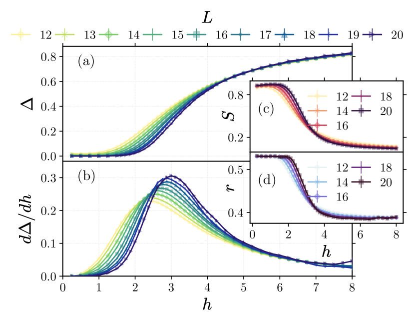
Characterizing the MBLT.– The main quantity we compute, new in the context of MBL, is the Schmidt gap. For two chain halves (or as close to for odd ), and , as shown in Fig. 1(a), an eigenvector’s reduced density matrix is for a particular sample of the random fields. The disorder-averaged Schmidt gap is then defined as , where , refer to the largest eigenvalues of the reduced density matrix , denotes average over eigenstates and denotes the average over many samples. The Schmidt gap has previously been shown to act as an order parameter for quantum phase transitions De Chiara et al. (2012); Bayat et al. (2014). We explore the possibility of using it for characterizing the MBLT. Unlike entanglement entropy, the Schmidt gap ignores most of the spectrum of , describing only the relationship between the two dominant states across the cut. This is pertinent in light of the recent finding that while the Schmidt values decay polynomially in the MBL phase Serbyn et al. (2016), finite size corrections are stronger for small Schmidt values. In the ergodic phase we expect strong entanglement to produce multiple, equally likely orthogonal states, thus . In the MBL phase, however, a single dominant state should appear on either side of the cut, with rising towards 1 as , implying a tensor product. This behaviour is shown in Fig. 2(a) and becomes becomes sharper with increasing . To see this more vividly, we plot the derivative of with respect to in Fig. 2(b). The derivative has a peak at , which not only becomes more pronounced but also shifts to the right with . We infer this to be the finite size precursor to the transition point, which suggests that in the thermodynamic limit, , the derivative of the Schmidt gap diverges at the MBLT and asymptotically approaches the transition point .
For reference, we consider the normalised half chain entropy, widely employed to herald the MBLT Pal and Huse (2010); Nandkishore and Huse (2015); Luitz et al. (2015); Ponte et al. (2015); Khemani et al. (2016, 2017). The von Neumann entropy of subsystem is defined as . This is normalized by the Page entropy Page (1993), , with , the Hilbert space dimensions of subsystems and , yielding the disorder-averaged . is the expected entropy for a subsystem of a random pure state; since these overwhelmingly have entropy that scales as their enclosed volume, gives a measure of how far has departed towards area law behaviour. In Fig. 2(c) the behaviour of across the MBLT is shown. In the ergodic phase its value approaches (showing the volume law), whereas in the MBL phase it falls to (representing the area law), as expected.
For reference we also compute the mean energy level spacing ratio, . For energy eigenvalues , with gaps , this is defined as . In the ergodic phase, energy level repulsion yields statistics for that match those of Gaussian Orthonormal Ensemble (GOE) random matrices Atas et al. (2013) with . In the MBL phase however, the eigenenergies are no longer correlated, and the energy level are simply spaced according to Poisson statistics, giving . In Fig. 2(d) the behaviour of is shown across the MBLT, clearly varying between these two statistical regimes. For all of these quantities, we average over between 10000 for and 1000 for samples of random fields, and compute errors using statistical bootstrapping across these samples.
Scaling.– The behaviour in Figs. 2(a)-(b) suggests that the MBLT is a continuous transition in which a diverging length scale emerges near the transition point, consistent with Pal and Huse (2010). In order to estimate the exponent , finite size scaling analysis Fisher and Barber (1972) has previously been employed for various quantities, including the entanglement entropy . These analyses, based on exact numerical methods, find Kjäll et al. (2014); Luitz et al. (2015); Khemani et al. (2017), contradicting the CCFS/CLO bound. A recently proposed explanation Khemani et al. (2017), suggests that there are two universality classes at play here, with that of inter-sample randomness not yet dominant for the system sizes studied.
In order to estimate for both models we consider the following finite size scaling ansatz,
| (2) |
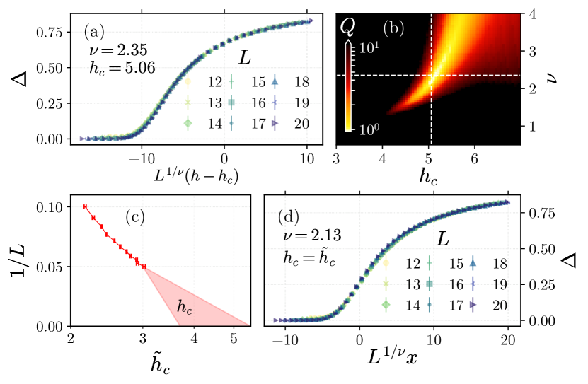
where is an unspecified function and is ideally the scaled coordinate . Given the ansatz of Eq. 2, one can then find the best fit of and , using an objective function quantifying quality. We use such a quality measure, , as refined in Houdayer and Hartmann (2004), which is discussed in the supplementary material. In Fig. 3(a) we show optimal data collapse of for various , which is found to occur for and . Remarkably, this value for is consistent with the CCFS/CLO bound, in contrast to finite size scaling analyses for and , which previous studies Kjäll et al. (2014); Luitz et al. (2015); Khemani et al. (2017) have generally shown to yield values of – a finding also reproduced in our analyses (data not shown). We show the quality of collapse, , for all possible combinations of and in Fig. 3(b), the minimum point of which defines the best fit values of and . To define errors on and , we perform the scaling with various subsets of data (see supplementary material) and compute the variance among all those which achieve a good quality.
The critical we find with is slightly higher than that generally reported. One possible explanation is that a lower effective fits best with a lower effective , a relation that can be seen in Fig. 3(b). Thus it is possible that in other studies using and , where , is artificially lower due to the finite size effects. We note that a standard method of extracting independently – plotting the pseudo-critical points against inverse length, shown in Fig. 3(c) – does not give a decisive value for the real critical point. In fact would seem to be a lower bound on the transition point , with a value between 4.5 and 5.5 more consistent. Additionally, if one were to identify an intersection point for all lengths in Fig. 2 – which should occur at as implied by Eq. (2) – this would also be at . In contrast, the point of intersection for and shifts significantly as increases - implying a deviation from the finite size ansatz. As a final cross-validation, to estimate independently from , we take the pseudo-critical points directly to define the scaled coordinate , and find the best quality of fit, , solely as a function of . This approach yields – in accordance with the first estimate – for which data collapse is shown in Fig. 3.
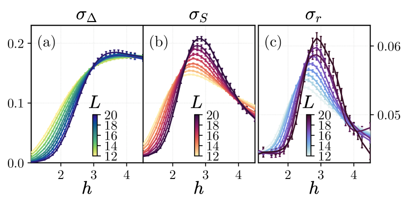
Sample Fluctuations.– In order to understand why the Schmidt gap is more successful than typical quantities, we study the fluctuation of , and between samples. Motivated by Ref. Khemani et al. (2017), we consider how the size of these fluctuations scales with . We define the standard deviations as , and , with the variance taken across samples. These are shown across the MBLT for various system sizes in Figs. 4(a-c). All three quantities must lie between 0 and 1, thus their standard deviation is capped at 0.5. As the figures show however, the peaks of and are both still rising significantly with and not yet saturated, whereas the peak of is almost constant. The implication is that for and , the effect of the small system sizes is to suppress the amount of fluctuations driven by the true disorder. On the other hand, changing the length seems to have little effect on – suggesting that it already experiences the full, disorder driven, thermodynamic-limit fluctuations. A possible explanation is that finite size effects are dominantly confined to the smaller Schmidt coefficients, which still contribute significantly to .
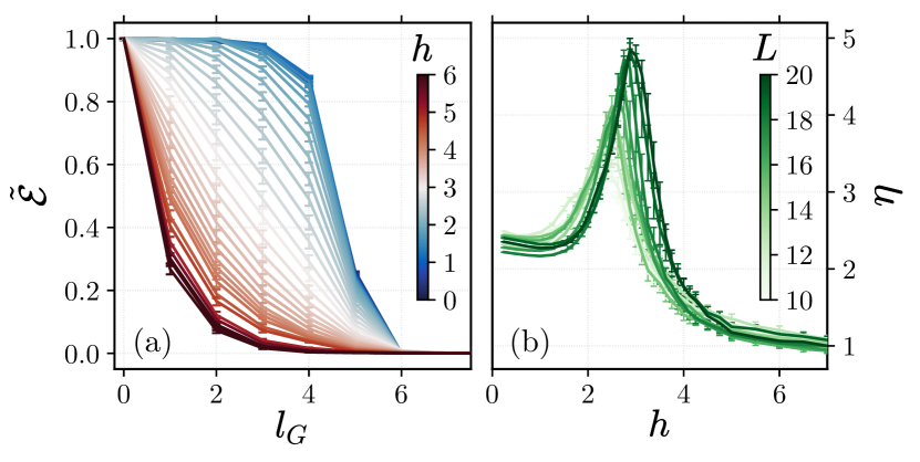
Entanglement length.– The nature of the diverging length scale , in the context of MBLT, is mysterious and a physical picture is lacking. To shed light on this, we introduce an entanglement length, as previously used for detecting the Kondo screening cloud Bayat et al. (2010, 2012). Specifically, we consider the entanglement between a small subsystem , here a single spin, and an environment , separated by a gap of length , a geometry shown in Fig. 1(b). The reduced state of the two blocks is , where is removes the spins not in or . We use the logarithmic negativity Peres (1996); Horodecki et al. (1996); Lee et al. (2000); Vidal and Werner (2002); Plenio (2005) to quantify the entanglement between systems and , defining , with the partial transpose, and the trace norm. Since we are only concerned with the relative decay of entanglement we also define the normalized entanglement as . This naturally gives information about bipartite entanglement over a range of scales, unlike the two-site concurrence for example (which quickly goes to zero for large separation), and unlike the widely used entanglement entropy (which cannot quantify the entanglement of mixed states – which inevitably arise when looking at two subsystems of a larger state). In the ergodic phase, due to volume law entanglement, the eigenstates are highly multipartite entangled between their spins. This implies that any reduced state of two small blocks is close to the identity and thus very weakly entangled. From this two features can be inferred: i) is initially expected to decay slowly with increasing , and ii) must go to zero as . Since this precludes a linear type decay, it is expected that there is a distance at which rapidly decays - indeed we find this to be the case, with a sharp drop-off when half the system is traced out, i.e. . In the MBL phase, however, will be weakly entangled with only spins close to it, and thus should decay quickly even for small . In Fig. 5(a) we plot as a function of for various disorder strengths in a chain of length . As is clear from the figure the location of the main drop in varies significantly with . While in the ergodic phase this decay is concentrated at , in the MBL phase it is concentrated at . Interestingly, at the pseudo-critical point, ( for , see Fig. 2(b)), entanglement decays close to linearly — each spin lost contributes equally to the entanglement, implying that the bipartite entanglement is equally spread over many sites. This fits with a picture of a self-similar structure of entangled clusters Potter et al. (2015); Khemani et al. (2016). The detailed behaviour of as a function of system size can be found in the supplementary material.
To extract a length scale from we define a length, , from the maximum inverse gradient as such:
| (3) |
Assuming the fastest decay is exponential-like, this quantity naturally arises from expressions of the form . This is a more robust way of finding an exponential fit in the region of the most rapid decay of , or a more general fit for the full behaviour. At the transition point, where decays linearly, takes its maximum value, since the gradient is always small, or equivalently, a very slow exponential fit is needed.
The behaviour of as a function of for varying is shown in Fig. 5(b), in which it can be seen to sharply peak at for each across the critical region, – evidence that the diverging length scale is closely captured by the length . In the supplementary material we show that taking the initial block as 2 spins yields almost identical results. A plausible explanation for the increase in as one approaches the MBLT from the ergodic side is that proximal spins become off-resonant so that bonding (bipartite entanglement) takes place at increasingly longer scales – a process that is not possible if the spins are part of a large multi-partite entangled block. We note several interesting approaches that made use of the two site concurrence Bera and Lakshminarayan (2016); Iemini et al. (2016) or mutual information De Tomasi et al. (2017), which despite revealing other interesting features, such as scaling, do not show a divergence in the localization length from both sides of the transition. An alternative approach to identifying the diverging length scale on the ergodic side based on the entanglement spectrum has been recently developed in Ref. Pietracaprina et al. (2016). It is an interesting open question whether that length is related to the entanglement length proposed here.
Conclusions.– In this letter we have explored the MBLT using the Schmidt gap and the entanglement length. We show that the Schmidt gap not only exhibits scaling at the MBLT, but does so with a critical exponent , compatible with analytic predictions. This compatibility is absent in all quantities studied with exact numerical methods thus far, a fact that we attribute to the presence of significant finite size effects which the Schmidt gap is less sensitive to. We have also considered an entanglement length computed using the logarithmic negativity across two disjoint blocks, which yields a diverging length scale at the MBLT.
Acknowledgements.
Acknowledgements.– JG acknowledges funding from the EPSRC Center for Doctoral Training in Delivering Quantum Technologies at UCL. AB and SB acknowledge the EPSRC grant EP/K004077/1. SB acknowledges financial support by the ERC under Starting Grant 308253 PACOMANEDIA.References
- Anderson (1958) P. W. Anderson, Phys. Rev. 109, 1492 (1958).
- Basko et al. (2006) D. M. Basko, I. L. Aleiner, and B. L. Altshuler, Ann. Phys. 321, 1126 (2006), ISSN 0003-4916.
- Imbrie (2016a) J. Z. Imbrie, Phys. Rev. Lett. 117, 027201 (2016a).
- Imbrie (2016b) J. Z. Imbrie, Journal of Statistical Physics 163, 998 (2016b).
- Luitz and Lev (2016) D. J. Luitz and Y. B. Lev, arXiv:1610.08993 (2016).
- Nandkishore and Huse (2015) R. Nandkishore and D. A. Huse, Annu. Rev. Condens. Matter Phys. 6, 15 (2015).
- Huse et al. (2014) D. A. Huse, R. Nandkishore, and V. Oganesyan, Phys. Rev. B 90, 174202 (2014).
- Sims and Stolz (2013) R. Sims and G. Stolz, arXiv:1312.0577 (2013).
- Bardarson et al. (2012) J. H. Bardarson, F. Pollmann, and J. E. Moore, Phys. Rev. Lett. 109, 017202 (2012).
- Pal and Huse (2010) A. Pal and D. A. Huse, Phys. Rev. B 82, 174411 (2010).
- Yao et al. (2015) N. Y. Yao, C. R. Laumann, and A. Vishwanath, arXiv:1508.06995 (2015).
- Vasseur et al. (2015) R. Vasseur, S. A. Parameswaran, and J. E. Moore, Phys. Rev. B 91, 140202 (2015).
- Serbyn et al. (2014) M. Serbyn, M. Knap, S. Gopalakrishnan, Z. Papić, N. Y. Yao, C. R. Laumann, D. A. Abanin, M. D. Lukin, and E. A. Demler, Phys. Rev. Lett. 113, 147204 (2014).
- Schreiber et al. (2015) M. Schreiber, S. S. Hodgman, P. Bordia, H. P. Lüschen, M. H. Fischer, R. Vosk, E. Altman, U. Schneider, and I. Bloch, Science 349, 842 (2015), ISSN 0036-8075, 1095-9203.
- Smith et al. (2016) J. Smith, A. Lee, P. Richerme, B. Neyenhuis, P. W. Hess, P. Hauke, M. Heyl, D. A. Huse, and C. Monroe, Nature Phys. 12, 907 (2016), ISSN 1745-2473.
- Serbyn et al. (2013) M. Serbyn, Z. Papić, and D. A. Abanin, Phys. Rev. Lett. 111, 127201 (2013).
- Nandkishore et al. (2014) R. Nandkishore, S. Gopalakrishnan, and D. A. Huse, Phys. Rev. B 90, 064203 (2014).
- Chandran et al. (2015a) A. Chandran, I. H. Kim, G. Vidal, and D. A. Abanin, Phys. Rev. B 91, 085425 (2015a).
- Ros et al. (2015) V. Ros, M. Müller, and A. Scardicchio, Nucl. Phys. B 891, 420 (2015), ISSN 0550-3213.
- Monthus (2016) C. Monthus, J. Stat. Mech. Theor. Exp 2016, 033101 (2016), ISSN 1742-5468.
- Friesdorf et al. (2015) M. Friesdorf, A. H. Werner, W. Brown, V. B. Scholz, and J. Eisert, Phys. Rev. Lett. 114, 170505 (2015).
- Serbyn et al. (2016) M. Serbyn, A. A. Michailidis, D. A. Abanin, and Z. Papić, Phys. Rev. Lett. 117, 160601 (2016).
- Wahl et al. (2016) T. B. Wahl, A. Pal, and S. H. Simon, arXiv:1609.01552 (2016).
- Zhang et al. (2016) C. Zhang, F. Pollmann, S. L. Sondhi, and R. Moessner, arXiv:1608.06411 (2016).
- Žnidarič (2016) M. Žnidarič, Phys. Rev. Lett. 117 (2016).
- Devakul et al. (2017) T. Devakul, V. Khemani, F. Pollmann, D. Huse, and S. Sondhi, arXiv:1702.07721 (2017).
- Luitz et al. (2015) D. J. Luitz, N. Laflorencie, and F. Alet, Phys. Rev. B 91, 081103 (2015).
- Ponte et al. (2015) P. Ponte, Z. Papić, F. Huveneers, and D. A. Abanin, Phys. Rev. Lett. 114, 140401 (2015).
- Khemani et al. (2016) V. Khemani, S. P. Lim, D. N. Sheng, and D. A. Huse, arXiv:1607.05756 (2016).
- Khemani et al. (2017) V. Khemani, D. N. Sheng, and D. A. Huse, arXiv:1702.03932 (2017).
- Jian and Yao (2017) S.-K. Jian and H. Yao, arXiv:1703.02051 (2017).
- Chayes et al. (1986) J. T. Chayes, L. Chayes, D. S. Fisher, and T. Spencer, Phys. Rev. Lett. 57, 2999 (1986).
- Chandran et al. (2015b) A. Chandran, C. R. Laumann, and V. Oganesyan, arXiv:1509.04285 (2015b).
- De Chiara et al. (2012) G. De Chiara, L. Lepori, M. Lewenstein, and A. Sanpera, Phys. Rev. Lett. 109, 237208 (2012).
- Lepori et al. (2013) L. Lepori, G. De Chiara, and A. Sanpera, Phys. Rev. B 87, 235107 (2013).
- Bayat et al. (2014) A. Bayat, H. Johannesson, S. Bose, and P. Sodano, Nat. Commun. 5 (2014).
- Peres (1996) A. Peres, Phys. Rev. Lett. 77, 1413 (1996).
- Horodecki et al. (1996) M. Horodecki, P. Horodecki, and R. Horodecki, Phys. Lett. A 223, 1 (1996), ISSN 0375-9601.
- Lee et al. (2000) J. Lee, M. S. Kim, Y. J. Park, and S. Lee, J. Mod. Opt. 47, 2151 (2000), ISSN 0950-0340.
- Vidal and Werner (2002) G. Vidal and R. F. Werner, Phys. Rev. A 65, 032314 (2002).
- Plenio (2005) M. B. Plenio, Phys. Rev. Lett. 95 (2005).
- Wichterich et al. (2009) H. Wichterich, J. Molina-Vilaplana, and S. Bose, Phys. Rev. A 80, 010304 (2009).
- Wichterich et al. (2010) H. Wichterich, J. Vidal, and S. Bose, Phys. Rev. A 81, 032311 (2010).
- Nobili et al. (2015) C. D. Nobili, A. Coser, and E. Tonni, J. Stat. Mech. Theor. Exp. 2015, P06021 (2015), ISSN 1742-5468.
- Coser et al. (2016a) A. Coser, E. Tonni, and P. Calabrese, J. Stat. Mech. Theor. Exp. 2016, 033116 (2016a), ISSN 1742-5468.
- Coser et al. (2016b) A. Coser, E. Tonni, and P. Calabrese, J. Stat. Mech. Theor. Exp. 2016, 053109 (2016b), ISSN 1742-5468.
- Bayat et al. (2010) A. Bayat, P. Sodano, and S. Bose, Phys. Rev. B 81, 064429 (2010).
- Bayat et al. (2012) A. Bayat, S. Bose, P. Sodano, and H. Johannesson, Phys. Rev. Lett. 109, 066403 (2012).
- Dalcin et al. (2011) L. D. Dalcin, R. R. Paz, P. A. Kler, and A. Cosimo, Adv. Water Resour. 34, 1124 (2011), ISSN 0309-1708.
- Hernandez et al. (2005) V. Hernandez, J. E. Roman, and V. Vidal, ACM Trans. Math. Softw. 31, 351 (2005), ISSN 0098-3500.
- Page (1993) D. N. Page, Phys. Rev. Lett. 71, 1291 (1993).
- Atas et al. (2013) Y. Y. Atas, E. Bogomolny, O. Giraud, and G. Roux, Phys. Rev. Lett. 110, 084101 (2013).
- Fisher and Barber (1972) M. E. Fisher and M. N. Barber, Phys. Rev. Lett. 28, 1516 (1972).
- Kjäll et al. (2014) J. A. Kjäll, J. H. Bardarson, and F. Pollmann, Phys. Rev. Lett. 113, 107204 (2014).
- Houdayer and Hartmann (2004) J. Houdayer and A. K. Hartmann, Phys. Rev. B 70, 014418 (2004).
- Potter et al. (2015) A. C. Potter, R. Vasseur, and A. Parameswaran, S., Phys. Rev. X 5, 031033 (2015).
- Bera and Lakshminarayan (2016) S. Bera and A. Lakshminarayan, Physical Review B 93, 134204 (2016).
- Iemini et al. (2016) F. Iemini, A. Russomanno, D. Rossini, A. Scardicchio, and R. Fazio, Physical Review B 94, 214206 (2016).
- De Tomasi et al. (2017) G. De Tomasi, S. Bera, J. H. Bardarson, and F. Pollmann, Phys. Rev. Lett. 118, 016804 (2017).
- Pietracaprina et al. (2016) F. Pietracaprina, G. Parisi, A. Mariano, S. Pascazio, and A. Scardicchio, arXiv:1610.09316 (2016).
- Sorge (2015) A. Sorge, pyfssa 0.7.6 (2015), URL https://doi.org/10.5281/zenodo.35293.
I Supplementary Material
I.1 Quality of Collapse
To find the quality of data collapse of scaled Schmidt data for a given and we use the ‘pyfssa’ program Sorge (2015). The underlying procedure, which is based on the method as refined in Houdayer and Hartmann (2004) is as follows. Assume we have data points (e.g the Schmidt gap, ) and their standard errors , where indexes the lengths and the disorder strengths . Since we assume that there is only a correlation length exponent, , we scale only the disorder strength as such: . A curve is then fitted through the data using least squares which yields the fitted points and their estimated errors . The quality can then be defined as a statistic based on the relative deviation from this fitted curve:
| (S1) |
with normalization accounting for the number of terms where the fitted curve is defined. This quantity is minimized when all the actual data lies close to the curve of best fit. In particular, when the deviations from the fit are approximately equal to the uncertainty in the fit, , which is generally what we find with the Schmidt gap .
Since finite size scaling is only strictly relevant close to the transition, and finite size effects may be too strong at very small lengths, there is also some freedom in how one selects the data to scale. Similarly to Luitz et al. (2015), we vary the size of the window around to select, the minimum of which to include data for, and also whether to include odd as well as even . The advantage of using Eq. (S1) is that the the combinations of the above which give statistically reasonable collapse can be objectively identified. The minimum is chosen such that increasing it does not significantly change the values of and found. One can then average over all parametrizations that achieve a ‘good’ value of (determined visually to be ) – yielding the plot in Fig. 3(b).
The different parametrizations above, as well as bootstrap sampling over disorder realizations, then yields a spread in the locations of and where the best value of is found. This allows an estimation of the error in and which takes into account both the collapse method and the random error.
I.2 Entanglement Length with Larger Block Size
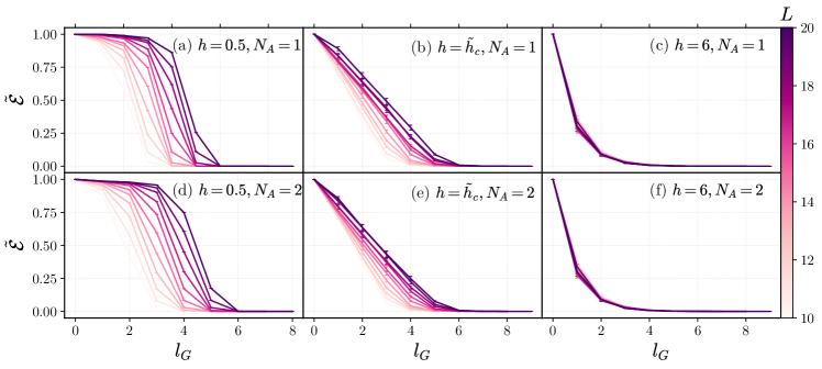
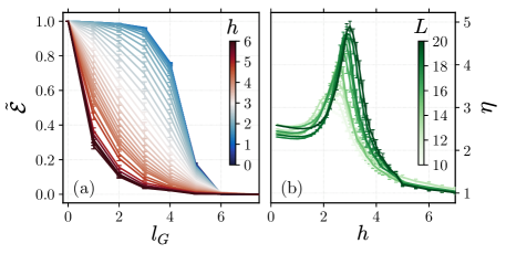
For completeness, we show here the equivalent of Fig. 5 taking instead the size of the block A to be 2. As can be seen in Fig. S1, this yields almost exactly the same shapes and plots, including a divergence of the length at the pseudo-critical points , which shift right with length .
I.3 Detailed Behaviour of the Disjoint Entanglement vs.
Finally, in Fig. S2, we show in detail the behaviour of the normalized disjoint entanglement as a function of , which sheds some light on the physical picture of the entanglement length. In the ergodic phase – left column, – one can see that the point of decay for shifts linearly to the right with system size , but the length scale of the decay (which is what captures) remains constant. In fact, the curves collapse onto each other with a shift of (not shown). In the localized phase – right column, – the decay of entanglement, and thus , is practically identical for all the lengths. At the transition point however – central column, taken as pseudo-critical points – the scale of decay stretches with system size. Lastly, we note that the difference between the two block sizes tested (upper row 1, lower row 2) is very minimal.
