Extending the Calibration of C IV-Based Single-Epoch Black Hole Mass Estimators for Active Galactic Nuclei^⋆

Abstract

We provide an updated calibration of C IV $\lambda 1549$ broad emission line-based single-epoch (SE) black hole (BH) mass estimators for active galactic nuclei (AGNs) using new data for six reverberation-mapped AGNs at redshift $z=0.005-0.028$ with BH masses (bolometric luminosities) in the range $10^{6.5}$–$10^{7.5}$ $M_{\odot}$ ($10^{41.7}$–$10^{43.8}$ erg s^-1). New rest-frame UV-to-optical spectra covering 1150–5700 Å for the six AGNs were obtained with the Hubble Space Telescope (HST). Multi-component spectral decompositions of the HST spectra were used to measure SE emission-line widths for the C IV, Mg II, and H$\beta$ lines as well as continuum luminosities in the spectral region around each line. We combine the new data with similar measurements for a previous archival sample of 25 AGNs to derive the most consistent and accurate calibrations of the C IV-based SE BH mass estimators against the H$\beta$ reverberation-based masses, using three different measures of broad-line width: full-width at half maximum (FWHM), line dispersion ($\sigma_{\rm line}$) and mean absolute deviation (MAD). The newly expanded sample at redshift $z=0.005-0.234$ covers a dynamic range in BH mass (bolometric luminosity) of $\log\ M_{\rm BH}/M_{\sun}=6.5-9.1$ ($\log\ L_{\rm bol}/$erg s^-1$=41.7-46.9$), and we derive the new C IV-based mass estimators using a Bayesian linear regression analysis over this range. We generally recommend the use of $\sigma_{\rm line}$ or MAD rather than FWHM to obtain a less biased velocity measurement of the C IV emission line, because its narrow-line component contribution is difficult to decompose from the broad-line profile.

1. INTRODUCTION

Understanding the cosmic growth of the supermassive black hole (BH) population and the coevolution of BH with their host galaxies is now recognized to be one of the essential ingredients for a complete picture of galaxy formation and evolution (see Ferrarese & Ford 2005 and Kormendy & Ho 2013). To probe the high-redshift BH population, and the evolution of the BH-galaxy scaling relations over cosmic time, it is essential to have reliable methods to determine black hole masses in distant active galactic nuclei (AGN) (Shen 2013).

The rest-frame UV C IV$\lambda 1549$ broad emission line is commonly used for BH mass estimates in high-redshift AGNs (i.e., $2\lesssim z\lesssim 5$) when single-epoch (SE) optical spectra are available. The method of deriving SE mass estimates based on broad-line widths and continuum luminosities in quasar spectra relies on reverberation-mapped (RM) AGN for its fundamental calibration. Achieving an accurate calibration of C IV-based SE BH mass estimators using the most reliable AGN BH mass estimates obtained from RM is thus important for improving the precision and accuracy of SE mass estimates for AGNs. Due to a lack of direct C IV RM measurements, however, the C IV SE calibration has been performed against the H$\beta$ RM-based BH masses, which is the best practical approach at present. Note that the H$\beta$ is so far the most studied and understood emission line in RM studies with many reliable H$\beta$-based RM results, which can thus be arguably regarded as the most reliable line for AGN BH mass measurements (see Shen 2013 for a related discussion).

Previously, Vestergaard & Peterson (2006, hereafter VP06) have provided a calibration of C IV-based BH mass estimators using a sample of low-redshift AGNs for which both H$\beta$ RM measurements and rest-frame UV spectra were available. Since then, the number of AGNs with BH mass estimates from RM has increased, as has the number of AGNs for which Hubble Space Telescope (HST) UV spectra have been obtained by the HST. Park et al. (2013, hereafter P13) have revisited the calibrations of C IV-based BH mass estimators by taking advantage of high-quality HST UV spectra for the reverberation-mapped AGN sample and using improved measurement methods. The P13 sample included 25 AGNs, of which six have estimated $M_{\rm BH}<10^{7.5}$ $M_{\odot}$ and only one has $M_{\rm BH}<10^{7.0}$ $M_{\odot}$. In order to improve the calibration of SE BH masses at the low end of the AGN mass range ($M_{\rm BH}\lesssim 10^{7.5}$ $M_{\odot}$), it is important to further expand the sample of AGNs having both RM measurements and HST UV spectroscopy. Similarly, a calibration of BH masses based on the broad Mg II $\lambda 2798$ emission line, another commonly used rest-frame UV line at intermediate redshifts, has also been performed (see, e.g., McLure & Jarvis 2002; Wang et al. 2009). As with C IV, there is also much room for improvement in the calibration of Mg II-based BH masses, and extending the calibration to a larger sample of AGNs over a wider dynamic range in BH mass is a high priority.

There have been several efforts in the literature to improve the calibration of C IV-based SE BH mass estimators, e.g., by taking advantages of the ratio of UV to optical continuum luminosities (color dependence; Assef et al. 2011), the ratio of FWHM to $\sigma_{\rm line}$ of C IV (line shape; Denney 2012), the peak flux ratio of the $\lambda 1400$ feature to C IV (Eigenvector 1; Runnoe et al. 2013a; Brotherton et al. 2015), and the C IV blueshift (Shen & Liu 2012; Coatman et al. 2017).

As an extension of our previous work (P13), this paper presents new HST UV and optical spectra of six reverberation-mapped AGNs with BH masses of $10^{6.5}$ to $10^{7.5}$ $M_{\odot}$. High quality spectra, quasi-simultaneously covering the C IV to H$\beta$ spectral regions with a consistent aperture size and slit width, were obtained with the Space Telescope Imaging Spectrograph (STIS). The new data enable a consistent comparison between the broad emission lines while minimizing measurement systematics due to time variability or aperture effects.

Using the new spectra, we provide updated calibrations of C IV-based SE BH mass estimators for three different measures of broad-line width: the full-width at half maximum (FWHM) and the line dispersion ($\sigma_{\rm line}$), which have been commonly used in previous work on SE mass estimates, and the mean absolute deviation (MAD), which was recently suggested by Denney et al. (2016b) to be a useful linewidth measure for virial mass estimation.

We use a Bayesian linear regression method, which is independently implemented for this work, to carry out the calibration of the C IV virial mass relation. Our method follows the work of Kelly et al. (2012) (see also Kelly 2007) using the Stan probabilistic programming language (Stan Development Team 2015a). The Bayesian methodology and model specifications for the linear regression analysis will be described in detail in a forthcoming paper (Park 2017, in preparation).

This paper is organized as follows. In Section missing 2, the calibration sample, HST observations, and data reduction procedures are described. In Section missing 3, we present measurements of the C IV, Mg II, and H$\beta$ emission lines and comparisons of their profiles. The new calibration of the SE virial mass estimators based on the FWHM, $\sigma_{\rm line}$, and MAD of the C IV line profile are presented in Section missing 4 with a comparison to previous calibrations and a test of methodological differences in the linear regression analysis. We also systematically compare our updated calibration with the corrected prescriptions in the literature for the C IV BH mass calibration described above. We summarize this work and provide discussions in Section missing 5. The following standard cosmological parameters were adopted to calculate distances: $H_{0}=70$ km s^-1 Mpc^-1, $\Omega_{\rm m}=0.30$, and $\Omega_{\Lambda}=0.70$, which is the same as used by P13.

2. Sample, HST Observations, And Data Reduction

The sample for this work is based on the sample of 25 AGNs (BH mass $\log M_{\rm BH}/M_{\odot}=7.0-9.1$, bolometric luminosity $\log\ L_{\rm bol}/$erg s^-1$=43.2-46.9$, redshift $z=0.009-0.234$) from P13, supplemented by six new AGNs at redshift $z=0.005-0.028$ that have low-mass BHs (i.e., $\log M_{\rm BH}/M_{\odot}=6.5-7.5$) from H$\beta$-based RM measurements and low bolometric luminosities (i.e., $\log\ L_{\rm bol}/$erg s^-1$=41.7-43.8$). The P13 sample contains reverberation-mapped AGNs with available archival HST spectra, selected by taking into account data quality, spectral coverage, and contamination of C IV by absorption features. The enlarged dynamic range in mass for the expanded sample enables us to calibrate the C IV SE virial relationship over almost three orders of magnitude in BH mass. The new targets have been selected from recent RM programs. These include Arp 151, Mrk 1310, NGC 6814, and SBS 1116+583A from the Lick AGN Monitoring Project 2008 campaign (Bentz et al. 2009b; Park et al. 2012b), Mrk 50 from the Lick AGN Monitoring Project 2011 campaign (Barth et al. 2011b), and the Kepler-field AGN Zw 229-015 (Barth et al. 2011a). Table 1 summarizes the properties of the P13 AGN sample and the six new objects presented in this work. Note that the virial factor $f$ with its uncertainty is adopted from Park et al. (2012a) and Woo et al. (2010, see also ) and applied to all RM BH masses (i.e., $\log f=0.71\pm 0.31$), which is consistent with previous measurements and also with direct measurements by Pancoast et al. (2012, 2014). The $f$ represents the dimensionless scale factor of order unity that depends on the detailed geometry, kinematics, and inclination of broad-line region (BLR), which is thus used to convert measured virial product into actual black hole mass ($M_{\rm BH}=f\times\rm VP_{\rm BH}$). The adopted uncertainty (0.31 dex) for the virial factor is derived from the scatter of the AGN $M_{\rm BH}-\sigma_{*}$ relation (0.43 dex), which gives an upper limit of random scatter of the virial factor itself after subtracting off in quadrature the assumed intrinsic scatter (0.3 dex) of the relation (see also the related discussion in Park et al. 2012b). Note that the virial factor uncertainty is the dominant portion of the error budget for the RM masses, since the measurement uncertainty propagated from the reverberation lags and H$\beta$ line widths is substantially smaller than this 0.31 dex uncertainty for individual AGNs (see Table 1).

For the six new AGNs, we obtained UV spectra with STIS as part of HST program GO-12922 (PI: Woo). In addition to the UV data, optical spectra were also obtained quasi-simultaneously (during the same HST visit) with a consistent slit width and aperture size. Note that temporal gaps between the end of optical exposures and the start of UV exposures were less than $\sim 6$ minutes. Individual exposures in and between UV gratings were obtained within a maximum temporal gap of $\sim 50$ minutes. The ability to obtain nearly simultaneous UV and optical spectra through a consistent aperture is a unique capability of the STIS instrument, and is essential in order to minimize possible systematic biases from AGN variability and different amounts of host galaxy and narrow-line region contributions.

We used the G140L, G230L, and G430L gratings with the 52x0.2 slit (i.e., a long slit of width 0$\farcs$2) to acquire a spectrum covering the Ly $\alpha$, C IV, Mg II, and H$\beta$ emission lines for each target. The consistent and small spectroscopic aperture has the benefit of minimizing the contamination from host-galaxy starlight. For the CCD G430L observations, we used the E1 aperture position to minimize losses due to the imperfect charge transfer efficiency as recommended in the STIS instrument handbook. Total integrations of 1170–1464 s for G140L, 627–1471 s for G230L, and 120–200 s for G430L respectively were split into two or three exposures depending on the grating, and dithered along the slit for optimal cleaning of cosmic-ray hits and bad pixels. The observations are summarized in Table 2. Note that the slit PA was not constrained, in order to maximize the HST scheduling opportunities. But the three grating data for each object were obtained in a single HST visit with the same orientation.

While we used the fully reduced data provided by the HST STIS pipeline for the UV gratings, we performed a custom reduction for the optical grating data from the raw science and reference files in order to improve the cleaning of cosmic-ray charge transfer trails in raw images from the badly degraded STIS CCD. Based on the standard reduction of the STIS pipeline, an additional cosmic-ray removal step was added to the processes employing the LA_COSMIC (van Dokkum, 2001) routine following the approach described by Walsh et al. (2013). The raw data for the optical G430L grating were first calibrated with the BASIC2D task including trimming the overscan region, bias and dark subtraction, and flat-fielding. Cosmic-rays and hot pixels were then cleaned with LA_COSMIC, and wavelength calibration was performed.

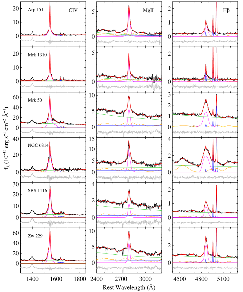
The dithered individual exposures for each grating were then aligned and combined using the IMSHIFT and IMCOMBINE PYRAF tasks. After that, one-dimensional spectra from each grating were extracted with the X1D task and then joined together to produce a final single spectrum by taking into account the flux and noise levels in overlapping regions around $\sim 1700$ Å and $\sim 3100$ Å. Following P13, we corrected the spectra for Galactic extinction using the values of $E(B-V)$ from Schlafly & Finkbeiner (2011) as listed in the NASA/IPAC Extragalactic Database (NED), and the reddening curve of Fitzpatrick (1999). Figure 1 shows the fully reduced and calibrated rest-frame spectra of the six AGNs.

3. Spectral Measurements

To measure the broad emission-line widths and the continuum luminosity adjacent to each broad line, we carried out a multi-component spectral decomposition analysis to the spectral region surrounding C IV $\lambda 1549$, Mg II $\lambda 2798$, and H$\beta$ $\lambda 4861$. A combination of these two observables, line width and continuum luminosity measured from a single-epoch spectrum, is commonly used to estimate BH masses via the SE BH mass estimators because they can be adopted as reasonable proxies for velocity of the broad-line gas clouds and the size of BLR (Kaspi et al., 2000, 2005; Bentz et al., 2006, 2009a, 2013), respectively. Following the standard approach that has been adopted in previous works (e.g., Shen et al., 2008, 2011), we measure monochromatic continuum luminosities at $1350$ Å, $3000$ Å, and $5100$ Å to compute SE virial masses from C IV, Mg II, and H$\beta$, respectively.

Our fits are based on a local decomposition of the spectral region around each broad line, rather than a global decomposition of the entire UV-optical spectrum. Owing to the complexity of the spectra and the large number of emission-line and continuum components that are present, we found that local decompositions are able to achieve a more precise fit to the data around each line than would be possible in a simultaneous, global fit to the full STIS spectrum (see later Section missing 3.5 for a discussion on the global versus local fits). The local spectral decomposition technique employed here is based on those by P13 and Park et al. (2015) and slightly updated and modified for the STIS data and the spectral region in question. Our spectral modeling method consists of separate procedures for continuum fitting and line emission fitting, applied independently to the C IV, Mg II, and H$\beta$ regions of the data. During fitting, model parameters are optimized using mpfit (Markwardt, 2009) in IDL. The model components and fitting details for each of the H$\beta$, Mg II, C IV line regions are described in the following subsections, and the decomposition results are given in Figure 2.

3.1. H$\beta$

We used the multi-component spectral decomposition code developed by Park et al. (2015) for modeling the H$\beta$ region of our STIS data. In brief, the code works by first simultaneously fitting a pseudocontinuum that consists of a single power-law, an Fe II template, and a host-galaxy template in the surrounding continuum regions of $4430-4770$ Å and $5080-5450$ Å, and then fitting the H$\beta$ emission line complex with Gauss-Hermite series functions (van der Marel & Franx, 1993; Cappellari et al., 2002) for one broad emission component (H$\beta$) and three narrow emission components (H$\beta$, [O III] $\lambda\lambda 4959,5007$), and two Gaussian functions for the nearby blended He II $\lambda 4686$ emission line after subtracting the best-fit pseudocontinuum model (see Park et al. 2015 and references therein for details of the measurement procedure) (see also Woo et al. 2006; Bennert et al. 2015; Runco et al. 2016). The H$\beta$ line widths, ${\rm FWHM}_{\rm H\beta}$ and $\sigma_{\rm H\beta}$, are measured from the best-fit broad line model (i.e., the Gauss-Hermite series function), and the continuum luminosity at $5100$ Å, $\lambda L_{5100\text{\rm\AA}}$, is measured from the best-fit power-law model.

Note that there are two differences between the method adopted here and the approach given by Park et al. (2015), specifically in the model components used for the Fe II emission and host-galaxy starlight. The template for host-galaxy starlight is excluded in this work because stellar absorption features, which is critical to achieve reliable host galaxy template fits, are not observable in the small-aperture STIS spectra. The minimal contribution of host-galaxy light and the relatively low signal-to-noise ratio and spectral resolution of the STIS optical data make it difficult to detect any host galaxy features in the optical data. Moreover, the fits did not converge when we included the host-galaxy starlight component in the model. As a rough check, we provide a crude estimate of an upper limit for host starlight contribution to the STIS spectra using the object, SBS 1116+583A, which shows the highest host galaxy fraction in the ground-based spectroscopic observations (see Park et al. 2012b; Barth et al. 2015) from our STIS sample. The host galaxy flux in the STIS spectrum can be roughly estimated by subtracting the AGN flux at $5100$ Å, which is obtained by subtracting off the HST imaging-based galaxy flux at $5100$ Å (Bentz et al., 2013) from the ground-based spectroscopic total flux at $5100$ Å (Park et al., 2012b), from the total flux at $5100$ Å of the STIS spectrum. The resulting host galaxy fraction in the STIS spectrum is found to be $\sim 31$%. Note that the other AGNs will have much lower contributions than this due to the lower host galaxy fractions shown by Park et al. (2012b) and Barth et al. (2015).

Available Fe II templates for the H$\beta$ region include empirically constructed monolithic templates by Boroson & Green (1992) and Véron-Cetty et al. (2004), a theoretical template by Bruhweiler & Verner (2008), and a semi-empirical multi-component template by Kovačević et al. (2010). After performing extensive tests using each of the templates and a linear combination of the templates for our STIS data, we opted to use the template by Kovačević et al. (2010) based on its overall performance as quantified by the $\chi^{2}$-statistics and residuals of the fits (see also Barth et al. 2013, 2015). As expected, the multi-component template generally performs better than monolithic templates, particularly for the objects showing strong Fe II emission. The Kovačević et al. (2010) template appears to be the best currently available for accurately fitting diverse Fe II emission blends in AGNs, by allowing for different relative intensities between five Fe II multiplet subgroups. To sum up, we follow the method described by Park et al. (2015) except that we used the template of Kovačević et al. (2010) instead of Boroson & Green (1992) for Fe II emission, and we omitted the host-galaxy starlight template from the fits.

3.2. Mg II

For the Mg II spectral region, we first fit a pseudocontinuum model in the surrounding continuum regions of $2450-2750$ Å and $2850-3100$ Å. The pseudocontinuum model is composed of a single power-law function representing the AGN featureless continuum, an Fe II emission template, and an empirical model for the Balmer continuum. We adopt the UV Fe II template from Tsuzuki et al. (2006), which is made from observations of I Zw 1. Using the template of Tsuzuki et al. (2006) is arguably better for modeling the Mg II line region than using that of Vestergaard & Wilkes (2001), because it contains semi-empirically constrained Fe II contribution underneath the Mg II line, while the template by Vestergaard & Wilkes (2001) has no Fe II flux at all under the Mg II line due to the difficulty of decomposing this spectral region.

Based on the investigations of Grandi (1982) and Wills et al. (1985) (see also Malkan & Sargent 1982 for the first practical measurement of the Balmer continuum shape), Dietrich et al. (2002, 2003) described a practical procedure for the Balmer continuum modeling in high-$z$ quasar spectra, which has become a standard practice for fitting the Balmer continuum. This empirical model assumes that the Balmer continuum is generated from partially optically thick gas clouds with uniform effective temperature ($T_{e}=15,000$ K) as

$$F_{\lambda}^{\rm BaC}(A,T_{e},\tau_{\rm BE})=AB_{\lambda}(T_{e})\left(1-e^{-\tau_{\rm BE}(\lambda/\lambda_{\rm BE})^{3}}\right),\lambda\leq\lambda_{\rm BE},$$ (1)

where $A$ and $\tau_{\rm BE}$ are normalized flux density and optical depth at the Balmer edge ($\lambda_{\rm BE}=3646$ Å), and $B_{\lambda}(T_{e})$ is the Planck function at the electron temperature $T_{e}$. At $\lambda>\lambda_{\rm BE}$, higher order Balmer lines using the relative intensity calculations from Storey & Hummer (1995) are used to represent the smooth rise to the Balmer edge. Many studies (e.g., Kurk et al. 2007; Wang et al. 2009; Greene et al. 2010; De Rosa et al. 2011, 2014; Ho et al. 2012; Shen & Liu 2012; Kokubo et al. 2014) have used variants of this method with slightly different ways of constraining the model parameter ranges based on the available data quality and spectral coverage. We found that if we treat all three parameters in the model ($A,T_{e},\tau_{\rm BE}$) as free parameters during fitting as done by Wang et al. (2009) and Shen & Liu (2012), they were very poorly constrained due to the degeneracy with the power-law continuum and Fe II emission blends.

Recently, Kovačević et al. (2014) suggested an improved way to constrain the normalization $A$, by taking into account a fact that $A$ can be obtained by calculating the sum of all intensities of higher order Balmer lines at the Balmer edge. We followed this procedure with slight modifications. The value of $A$ was separately determined from the intensity calculation using high order Balmer lines (up to 400) with the template line profile adopted from the best-fit H$\beta$ emission line model obtained above. The other parameters, $T_{e}$ and $\tau_{\rm BE}$, were then fitted simultaneously with the Fe II template and power-law function during the pseudocontinuum modeling. Note, however, that following the Dietrich approach, the temperature was finally fixed to be $15,000$ K and optical depth was allowed to vary between 0.1 and 2. We also independently checked that the constrained Balmer continuum component only exhibits marginal changes over temperature ranging from 10,000 K to 30,000K and optical depth varying from 0.1 to 2. Note that the resulting continuum luminosity estimates are consistent with each other within $\sim 0.04$ dex scatter.

After subtracting the best-fit pseudocontinuum model, the Mg II emission line was fitted using a linear combination of a sixth-order Gauss-Hermite series and a single Gaussian function to account for its full line profile, typically showing a more peaky core (i.e., narrower and sharper line peak) and more extended wings than a Gaussian profile, in the spectral region $\sim 2700-2900$ Å. We use the full line profile without a decomposition of narrow and broad components for line width measurements for UV lines in this work (the same approach adopted by P13), in contrast to H$\beta$, because no reliable and clear distinction between broad and narrow components in the UV lines is usually possible, and sometimes no narrow components of the UV lines are seen at all, although their presence is still uncertain and under debate. Thus, the Mg II line widths, ${\rm FWHM}_{\rm MgII}$ and $\sigma_{\rm MgII}$, are measured from the best-fit full line profile, and continuum luminosity at $3000$ Å, $\lambda L_{3000\text{\rm\AA}}$, is measured from the best-fit power-law function. During fitting, Galactic absorption lines such as Fe II $\lambda\lambda 2586,2600$, Mg II $\lambda\lambda 2796,2803$, and Mg I $\lambda 2852$ (cf. Savaglio et al. 2004) were masked out with exclusion windows.

3.3. C IV

Spectral measurements for the C IV line region in the previous archival sample of local 25 RM AGNs were described by P13. Here we focus on analysis of the 6 objects with newly obtained STIS data. We used the same methods as in P13 for consistency and to avoid additional systematic biases. We fit the AGN featureless continuum with a single power-law function, and we chose to omit a UV iron template (e.g., Vestergaard & Wilkes 2001) from the fits because no clear contribution of iron emission over the C IV region is observed. Although we performed a test including the UV iron template in the model as in P13, its contribution was too small to be constrained accurately with the template at least in our sample (see also Shen et al. 2008, 2011).

After the best-fit continuum model is subtracted, the C IV emission line is fitted with a linear combination of a sixth-order Gauss-Hermite series and a single Gaussian function. The contaminating nearby blended emission lines (e.g., N IV] $\lambda 1486$, Si II $\lambda 1531$, He II $\lambda 1640$, O III] $\lambda 1663$) are fitted simultaneously as well using up to two Gaussian functions for each line. Again, we use the combined model of one Gauss-Hermite function and one Gaussian function to fit the full line profile of C IV without decomposing it into broad and narrow components. The C IV line widths, ${\rm FWHM}_{\rm CIV}$ and $\sigma_{\rm CIV}$, are measured from the best-fit full line profile, and continuum luminosity at $1350$ Å, $\lambda L_{1350\text{\rm\AA}}$, is measured from the best-fit power-law function. Narrow absorption spikes are masked out using a $3\sigma$ clipping threshold during fitting, and broad absorption features around the line center are masked out manually with exclusion windows (see P13 and references therein for more details of the C IV measurement method and results for the archival sample).

3.4. Measurement uncertainty estimation

Uncertainties for the above spectral measurements are estimated with the Monte Carlo method used by Park et al. (2012b) and P13 (see also Shen et al. 2011; Shen & Liu 2012). For each spectral region, 1,000 mock spectra are generated by resampling the original spectra with the addition of Gaussian random noise based on the error spectrum for each object. We then measure line widths and luminosities from each of the mock spectra using the same measurement methods and take the standard deviation of the distribution of the measurements as the estimate of measurement uncertainty.

Typical uncertainty levels of line widths for all objects are found to be $\sim 2-4$% with a maximum of $\sim 17$% due to the high quality of the HST spectra. For continuum luminosity, we derive uncertainties of $\sim 1-2$% with a maximum of $\sim 6$%. These are small compared to the overall systematic mass uncertainty of $\sim 0.4$ dex in the SE virial method. Covariances between the measurement uncertainties of the line widths and luminosity for each object in a logarithmic scale are also estimated from the resulting distributions of the Monte Carlo simulations, which are given as ${\rm cov}(\log\lambda L_{\lambda},\log{\rm FWHM})=\rho\sigma(\log\lambda L_{\lambda})\sigma(\log{\rm FWHM})$ and ${\rm cov}(\log\lambda L_{\lambda},\log\sigma_{\rm line})=\rho\sigma(\log\lambda L_{\lambda})\sigma(\log\sigma_{\rm line})$ where ${\rm cov}$, $\rho$, and $\sigma$ are the covariance, correlation coefficient, and measurement uncertainty of the logarithms of the luminosity and line widths, respectively. Table 3 lists the line widths and luminosities for our sample along with the measurement uncertainties and their error correlation coefficients.

3.5. Continuum luminosities and emission-line widths

There are several issues in regard to measuring continuum luminosities and line widths accurately. It is important to take into account the Balmer continuum over the Mg II line region to accurately decompose the power-law continuum for luminosity measurements. Based on our investigation of the STIS data, the $\lambda L_{3000\text{\rm\AA}}$ values would be overestimated by $\sim 0.14$ dex on average if the Balmer continuum component is not accounted for, which is also consistent with the investigation of Shen & Liu (2012), who found $\sim 0.12$ dex systematic offset. This bias will then be propagated into final $M_{\rm BH}$ estimates by as much as a $\sim 0.07$ dex ($\sim 17$%) systematic offset if the Balmer continuum model is not included properly.

If the original Vestergaard & Wilkes (2001) Fe II template is used, FWHM ($\sigma_{\rm line}$) estimates are overestimated by $\sim 0.03$ ($0.07$) dex on average compared with results derived using the template of Tsuzuki et al. (2006). This will again be propagated into $M_{\rm BH}$ estimates by up to $\sim 0.06$ ($0.14$) dex of systematic offset, which is consistent with the result of Nobuta et al. (2012).

To make the maximum use of the wide spectral coverage of our STIS data, we have also performed extensive tests of global continuum fits covering C IV to H$\beta$ simultaneously. Using a more flexible double power-law model to represent the AGN featureless continuum, we fit a pseudocontinuum model including the Balmer continuum model and Fe II emission to many line-free continuum regions (see also, e.g., Shen & Liu 2012 and Mejía-Restrepo et al. 2016 for related recent work). The global continuum fits produced results consistent with the local continuum fits described in the previous sections, except that the global fits failed to constrain the Fe II emission on the red side of the Mg II regions for Arp 151 and Mrk 1310. This is probably because the double power-law model is not flexible enough to properly describe steep local slope changes around Mg II for these two objects, which is coming from intrinsic changes of spectral shapes and/or from strong internal reddening, along with the incompleteness of currently available UV Fe II templates across the regions. In any case, there is no significant improvement of the global fits compared to the local fits.

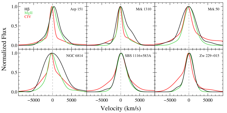
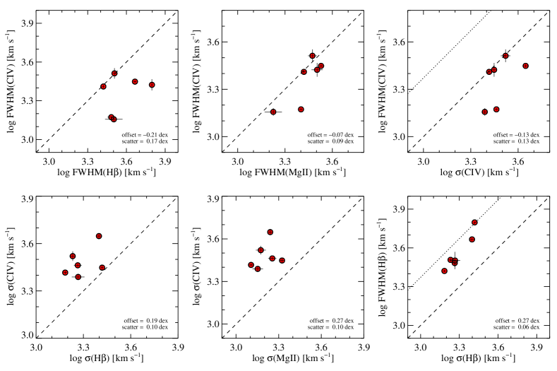
The simultaneous coverage of our STIS data also makes it possible to consistently compare the major UV and optical emission lines (C IV, Mg II, H$\beta$) without biases from intrinsic variability (Figure 3). The C IV profile shows on average more peaky cores with extended wings than those of the Mg II and H$\beta$ lines (see also Wills et al. 1993; Brotherton et al. 1994). There is no significant velocity offset between the line peaks of all the three emission lines. Figure 4 compares FWHM and $\sigma_{\rm line}$ line width measurements among the emission lines. Although it is hard to draw a clear picture due to small-number statistics, we use only our STIS sample of six AGNs in order to perform a consistent comparison between the line widths in quasi-simultaneously observed data. We find that the FWHM of C IV is on average smaller than that of H$\beta$ (and Mg II) FWHM, which may indicate that FWHM for C IV is not a good proxy for virial BLR velocity, probably due to contamination from a non-reverberating C IV core component (Denney, 2012). This contamination would be one of the biases correlated with Eigenvector 1 (EV1; Boroson & Green 1992) as discussed by Runnoe et al. (2013a, 2014) and Brotherton et al. (2015) who investigated and used the peak flux ratio of the $\lambda 1400$ feature to C IV, as a UV indicator of the EV1, to correct for the C IV-based BH masses. However, the interpretation is not straightforward. It could also be the case that the BLR geometry is different for the regions emitting these three lines, resulting in different individual virial factors ($f$) for each line (see also Runnoe et al. 2013b). On the other hand, $\sigma_{\rm CIV}$ is on average larger than $\sigma_{\rm H\beta}$, which is consistent with the simple virial expectation of stratified BLR structure and the shorter reverberation lags of C IV (Peterson & Wandel 1999; Kollatschny 2003), thus corroborating the use of $\sigma_{\rm line}$ over FWHM for C IV-based BH mass estimates. More detailed intercomparisons and systematic investigation of multi-line properties including more objects from the literature will be presented in a forthcoming paper.

4. Bayesian Calibration of C IV-based $M_{\rm BH}$ estimators

Now that we have the continuum luminosity and line width measurements from single-epoch spectra, we can perform a calibration of the C IV-based SE BH mass estimators against the H$\beta$ RM-based BH masses as fiducial baseline. We assume that the BH masses from H$\beta$ RM are the most reliable mass estimates available for these galaxies, and our goal is to find the combination of the SE measurements that most closely reproduces the RM mass scale, using the following equation:

$$\log\left(\frac{M_{\rm BH}^{\rm RM}}{M_{\odot}}\right) ~{}=~{} \alpha~{}+~{}\beta~{}\log\left(\frac{\lambda L_{1350{\rm\text{\AA}}}^{\rm SE}}{10^{44}~{}\rm erg~{}s^{-1}}\right)$$ (2)

$$~{}+~{} \gamma~{}\log\left(\frac{\varDelta V_{\rm CIV}^{\rm SE}}{1000~{}\rm km~{}s^{-1}}\right),$$

where $\varDelta V_{\rm CIV}^{\rm SE}=\rm FWHM^{\rm SE}_{\rm CIV}$ or $\sigma^{\rm SE}_{\rm CIV}$. This equation essentially expresses the virial relation $M_{\mathrm{BH}}\sim r_{\mathrm{BLR}}V^{2}/G$, assuming that BLR radius scales with AGN luminosity according to $r_{\mathrm{BLR}}\propto L^{\beta}$ and allowing for the virial exponent $\gamma$ to differ from the physically expected value of 2 in order to achieve the best fit.

Note that calibrations of the BH mass estimators based on the emission lines which have no direct reverberation measurements, e.g., C IV and Mg II, have been performed indirectly against the H$\beta$-based reverberation results for the same objects if available (e.g., VP06 and P13). Although there are a few direct (or in some cases tentative) reverberation results for the UV emission lines (e.g., Kaspi et al., 2007; Trevese et al., 2014, see also Shen et al. 2016a), most of the available reverberation studies have been done with the H$\beta$ line, which gives the most reliable AGN BH masses at present.

To perform the calibration, we adopt a Bayesian approach to linear regression analysis. An advantage of the Bayesian method over the traditional $\chi^{2}$-based is that by obtaining probability density functions (PDFs) for parameters of interest instead of just calculating a point estimate, it provides more reliable uncertainty estimates, incorporating all the error sources modeled and simply marginalizing over nuisance parameters. It is also easy to explore covariance between parameters from resulting joint probability distributions. Bayesian linear regression method outperforms other previous classical methods especially when the measurement error of independent variables is large and/or the sample size is small (see Kelly 2007).

For full Bayesian inference, we use the Stan probabilistic programming language (Stan Development Team, 2015a), which contains an adaptive Hamiltonian Monte Carlo (HMC; Neal 2012; Betancourt & Girolami 2013) No-U-Turn sampler (NUTS; Hoffman & Gelman 2014) as its sampling engine. This provides a simple implementation for specifying complex hierarchical Bayesian models and achieves good computational efficiency. We set up the Bayesian hierarchical model following Kelly et al. (2012) and implement it by referring to Gelman et al. (2013); Kruschke (2014); Stan Development Team (2015b). The practical details of the sampler and the model specification will be described in a separate paper describing the methodology (Park 2017, in preparation). As a brief summary, the $t$ distribution is adopted to obtain outlier-robust statistical inference following the investigation of Kelly et al. (2012) with an additional improvement of treating degrees-of-freedom in the $t$ model as a free parameter, instead of fixing it to be a pre-selected constant. Thus, the likelihood function, which is specifying the measurement, regression, and covariate distribution models, is built with the $t$ distributions, and the prior distributions are specified based on the suggestions by Barnard et al. (2000); Gelman et al. (2013); Kruschke (2014). Our Markov chain Monte Carlo (MCMC) simulations have been run via the PyStan package (v2.9.0; Stan Development Team 2016) with careful assessment of the convergence of the MCMC chains.

4.1. The single-epoch mass calibration

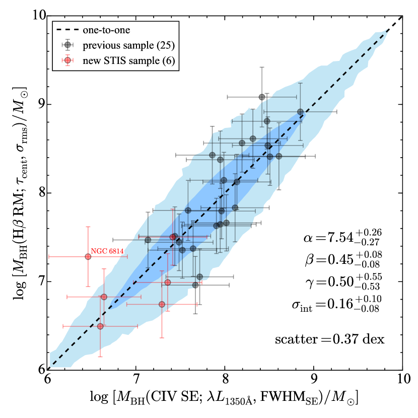
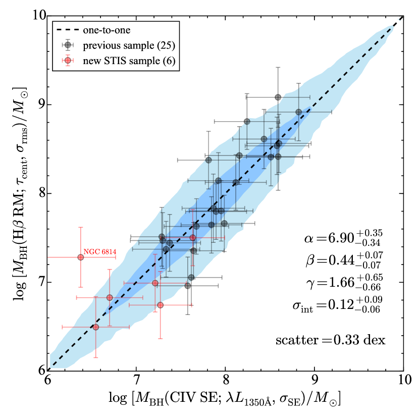
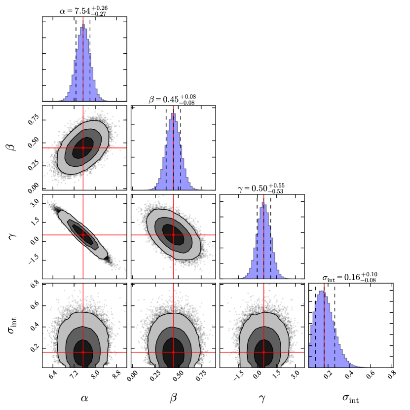
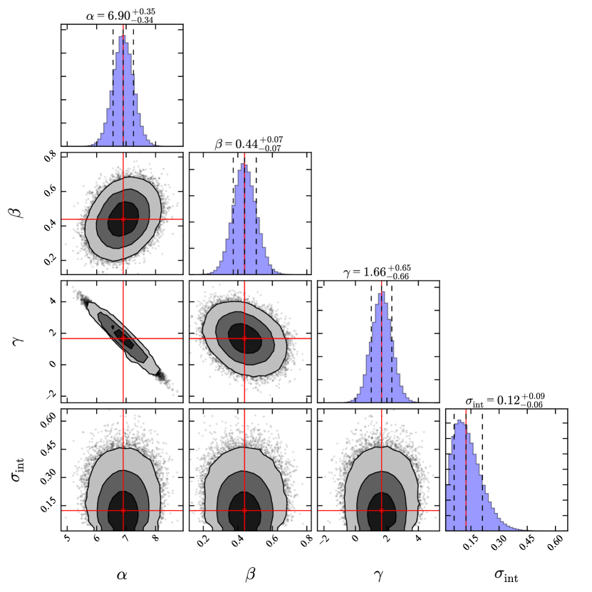
Figure 5 shows the results of calibration of C IV-based SE BH mass estimators against the H$\beta$-based RM masses using the full sample of 31 local RM AGNs with Equation 2, while Figure 6 presents corresponding marginal projections of each pair of parameters of interest with one-dimensional marginalized distributions from the full posterior distribution, from which parameter covariances are simply identifiable. We take the best-fit values and uncertainties of parameters of interest ($\alpha,\beta,\gamma,$ and $\sigma_{\rm int}$) from posterior median estimates and 68% posterior credible intervals as recommended by Kelly (2007) and Hogg et al. (2010).

In each panel of Figure 5, the two mass estimates (RM and SE) are fairly consistent. The overall scatter of the SE BH masses based on the calibrated equation using the C IV FWHM ($\sigma_{\rm line}$) compared to the RM BH masses are at the level of 0.37 dex (0.33 dex). This indicates in general quite good consistency, given the unavoidable object-to-object scatter of the virial factor $f$ (0.31 dex; Woo et al. 2010), since we are adopting a single ensemble average value of the $f$ factor for all objects.

To assess the resulting model fit to the data, we present the posterior predictive distribution (blue shaded contour), which is generated from simulations according to the fit parameters of the model, to check whether the posterior prediction reasonably well replicates the original observed data distribution. As can be seen, the 95% credible region depicted by the light blue filled contour describes most of the data distribution well, except for one outlier, NGC 6814. We have also calculated posterior predictive $p$-values by following the method of Chevallard & Charlot (2016) (see also Gelman et al. 2013 and PyMC User’s Guide). Using $\chi^{2}$ deviance as a discrepancy measure, the Bayesian $p$-value estimates are mostly $\sim 0.2$, ranging from 0.14 to 0.26 in this work, indicating successful model fits to the data. Note that there is a problem (e.g., misfit or inadequacy in the descriptive model) if the $p$-value is extreme, i.e., $<0.05$ or $>0.95$. All the calibration results performed in this work for various cases are listed in Table 4. Note that the presence of the single outlier, which is not very extreme, does not alter any of the conclusions and virtually the same result is obtained for give uncertainties if the outlier is removed.

The luminosity slope, $\beta$, is consistent with the photoionization expectation (i.e., 0.5) within uncertainties for both FWHM-based and $\sigma_{\rm line}$-based estimators. This may also imply that the size-luminosity relation for the UV 1350 Å continuum has a slope consistent with the relation for the optical 5100 Å continuum (e.g., $0.533^{+0.035}_{-0.033}$ by Bentz et al. 2013). The velocity slope, $\gamma$, for the $\sigma_{\rm line}$-based estimator is close to the virial expectation (i.e., 2) within uncertainties, while it is not the case for the FWHM-based, whose $\gamma$ value is consistent with zero, given the uncertainty interval. This is generally consistent with the calibration result based on C IV FWHM by Shen & Liu (2012), who found a much smaller slope (0.242) than 2, although their luminosity dynamic range probed is much higher than ours. And the $\sigma_{\rm line}$-based SE masses show overall less intrinsic and total scatter than the FWHM-based masses. Thus, this indicates that the C IV $\sigma$ is a better tracer of BLR velocity field than the C IV FWHM because it is closer to the virial relation and shows less scatter in mass estimates. These results are in overall agreement with Denney (2012) who found that the C IV FWHM is much more affected by a contaminating non-variable C IV core component (see also P13 and Denney et al. 2013 for related discussion and interpretation). The shallower velocity slopes (0.50, 1.66) than the virial expectation (2) would also be expected in part due to an additional dispersion of the measured line-of-sight velocities stemming from orientation dependence (see Shen & Ho 2014).

Our final best fits are as follows (see also Table 4):

$$\log\left[\frac{M_{\rm BH}{\rm(SE)}}{M_{\odot}}\right] ~{}=~{} {\bf 6.73}^{+0.07}_{-0.07}~{}+~{}{\bf 0.43}^{+0.06}_{-0.06}~{}\log\left(\frac{\lambda L_{1350{\rm\text{\AA}}}}{10^{44}~{}\rm erg~{}s^{-1}}\right)$$ (3)

$$~{}+~{} {\bf 2}~{}\log\left[\frac{\sigma(\textrm{{C~{}IV}})}{1000~{}\rm km~{}s^{-1}}\right]$$

with the overall scatter against RM masses of $0.33$ dex, which is defined by standard deviation of mass residuals $\varDelta=\log M_{\rm BH}{\rm(RM)}-\log M_{\rm BH}{\rm(SE)}$, and

$$\log\left[\frac{M_{\rm BH}{\rm(SE)}}{M_{\odot}}\right] ~{}=~{} {\bf 7.54}^{+0.26}_{-0.27}~{}+~{}{\bf 0.45}^{+0.08}_{-0.08}~{}\log\left(\frac{\lambda L_{1350{\rm\text{\AA}}}}{10^{44}~{}\rm erg~{}s^{-1}}\right)$$ (4)

$$~{}+~{} {\bf 0.50}^{+0.55}_{-0.53}~{}\log\left[\frac{\rm FWHM(\textrm{{C~{}IV}})}{1000~{}\rm km~{}s^{-1}}\right]$$

with the overall scatter against RM masses of $0.37$ dex. For the case of the $\sigma_{\rm line}$-based estimator, note that the value of $\gamma$ is fixed to be 2 (i.e., consistent with the virial expectation) in our final analysis because it is consistent with 2 within the uncertainty estimate when we treat it as a free parameter. Fixing $\gamma$ to the physically motivated value helps to avoid possible object-by-object biases and systematics due to small number statistics, and reduces the uncertainties of the other resulting regression parameters (see also P13). The overall scatter of the $\sigma_{\rm line}$-based calibration has virtually unchanged if we fix $\gamma=2$, while that of the FWHM-based calibration increases considerably if $\gamma$ is fixed to 2 (see Table 4).

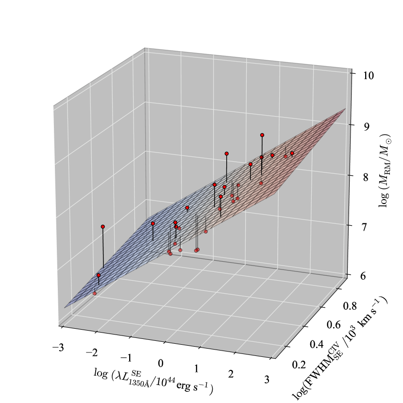
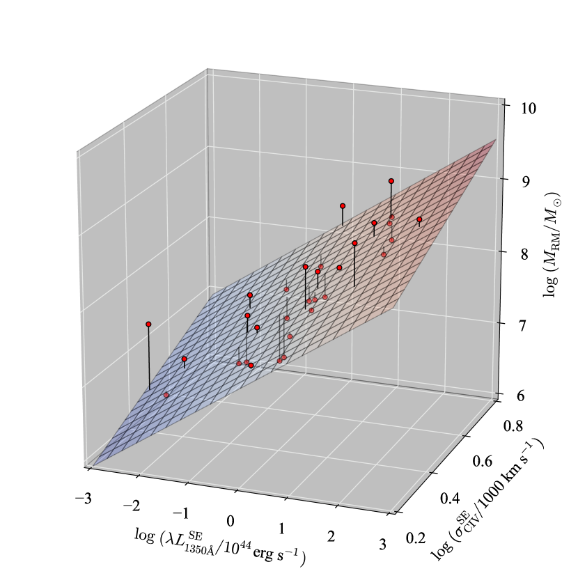
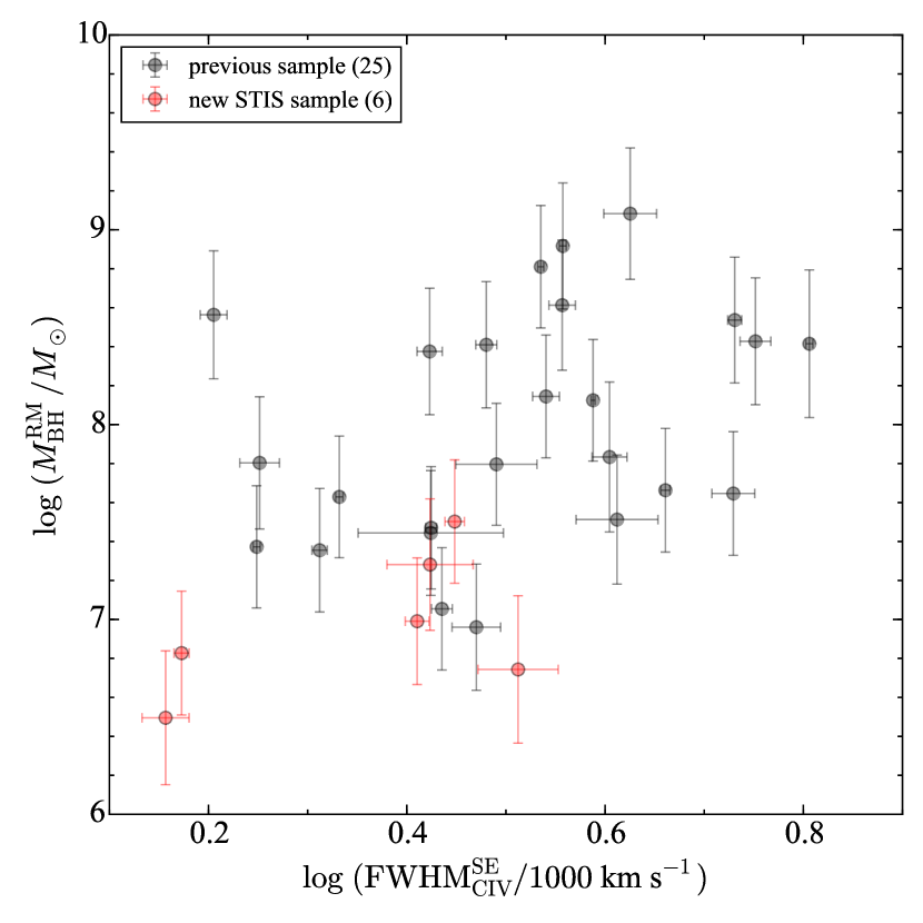
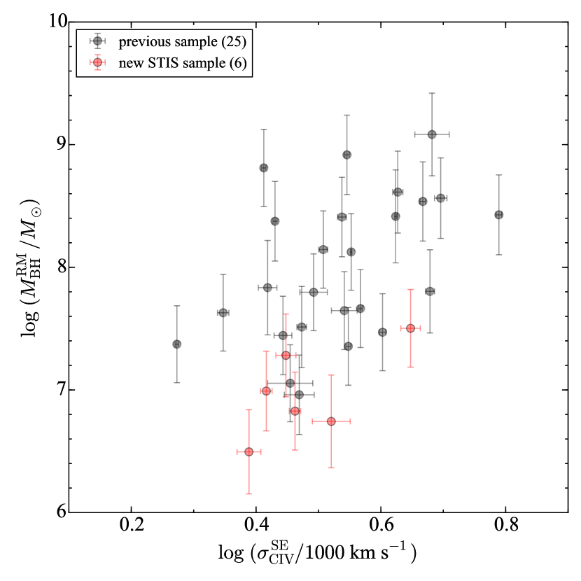
In Figure 7, we show the calibration results in a three-dimensional space of luminosity, velocity, and mass for clarity. There is a strong dependence of mass on luminosity, while there is much weaker dependence of mass on velocity, partly due to the small dynamic range of broad-line velocity in our sample. Especially for FWHM, the change of mass as a function of velocity is only marginal. As expected from the very small value of $\gamma$ for the FWHM-based estimator, it seems that C IV FWHM velocity characterization does not significantly add useful information to mass estimates, which is consistent with the result by Shen & Liu (2012) (see also discussions on the importance of line width information by Croom 2011 and Assef et al. 2012). It would thus be possible to achieve a comparable level of accuracy in mass estimates using the luminosity information only, at least for the present sample. This much weaker dependence of FWHM on mass than $\sigma_{\rm line}$ can also be observed from the projected RM mass-SE velocity plane in Figure 8, which reinforces that $\sigma_{\rm line}$ is a better velocity width measurement for C IV line than FWHM. Thus, we generally recommend to use the $\sigma_{\rm line}$-based C IV SE $M_{\rm BH}$ estimator than the FWHM-based since it is closer to virial relation and shows a better correlation and less scatter against the RM masses.

In this work (i.e., Equations 3, 4, and Table 4), we have used the virial factor, $\log f=0.71$, taken from Park et al. (2012a) and Woo et al. (2010) for a consistent comparison with the previous result of P13. If one wants to use a more recent value of the virial factor for BH mass estimates, e.g., the recently updated virial factor, $\log f=0.65$, from Woo et al. (2015), one can simply subtract the difference ($0.06$) between the adopted virial factors from the normalization, $\alpha$, of all the calibration results in this work. Our results can similarly be rescaled to any other adopted value for virial factor $f$.

4.2. Comparison with P13

The final best-fit calibrated equations (3 and 4) are very similar to those of our previous work (see their equations 2 and 3 of P13). If we compare the two mass estimates based on both estimators using the same measurements of our sample, there are very small offsets ($0.02-0.03$ dex) with small scatters of $\sim 0.09$ dex for both FWHM-based and $\sigma_{\rm line}$-based masses, which are mostly coming from slight differences in the slopes between P13 and this work. Although the changes in the adopted virial relation are modest, it is worth noting that this work directly extends the applicability of the C IV-based $M_{\rm BH}$ estimators toward lower BH masses ($\sim 10^{6.5}$ $M_{\sun}$) than were present in the P13 sample.

4.3. Comparison with other linear regression methods

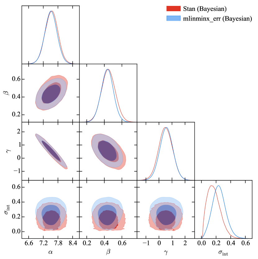
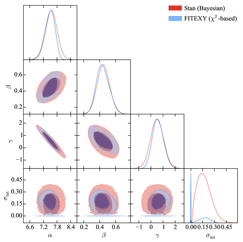
Advantages of the adopted statistical model using Stan in this work are 1) using the outlier-robust $t$-distribution as an alternative to the normal distribution for error distributions, and 2) modeling the intrinsic distribution of covariates explicitly with a multivariate $t$-distribution. To check the performance of our model, we here provide a comparison of results by performing the same regression work with other available methods (i.e., mlinmix_err and FITEXY).

Figure 9 compares the resulting posterior distributions of parameters obtained from three different regression methods for the same data (i.e., calibration of the FWHM-based estimator using the full sample of 31 local RM AGNs as obtained above). The Stan Bayesian model implemented for this work (Park 2017 in preparation) uses the Student-$t$ distributions for measurement errors, intrinsic scatter, and the covariate distribution model. The mlinmix_err method, a Bayesian linear regression code developed by Kelly (2007), employs a normal mixture model for covariate distribution and assumes Gaussian distributions for measurement errors and intrinsic scatter. The FITEXY method, a widely used traditional $\chi^{2}$-based linear regression method (Tremaine et al. 2002; see also Park et al. 2012a and references therein), also uses Gaussian distributions for measurement errors and intrinsic scatter, but has no model specified for the covariate distribution, and does not take into account possible correlations between measurement errors.

The left panel in Fig. 9 shows an overall consistency of the results between the Bayesian methods, Stan and mlinmix_err, except for the distributions of intrinsic scatter. The quite strong difference of the $\sigma_{\rm int}$ distributions is expected because Stan uses $t$-distributed intrinsic scatter while mlinmix_err uses normally distributed intrinsic scatter. By definition, the $\sigma_{\rm int}$ of the $t$-distribution is smaller than that of the Gaussian distribution due to the broader tails of the $t$-distribution (see Kelly et al. 2012 and Park 2017 in preparation). Another noticeable difference between the posterior distributions is that widths of the probability distributions for regression parameters obtained from Stan are slightly wider than those from mlinmix_err. Although not significant, this seems to be indicating more reliable uncertainty estimates with Stan, probably due to the flexibility of the adopted $t$-distributions with degrees-of-freedom parameters. Note that the $t$-distribution widely ranges from the Cauchy distribution to the normal distribution as well with a varying degrees-of-freedom parameter, but the number of Gaussian components for the normal mixture model used in mlinmix_err is fixed to be a constant (e.g., three by default, although a few Gaussians are usually well enough to obtain a reasonable description of observed distributions of many astronomical samples and data, as it is in this work).

The right panel in Fig. 9 also shows a overall consistency between the resulting distributions of the Bayesian Stan and the $\chi^{2}$-based FITEXY method. However, underestimates of the parameter uncertainties from FITEXY are a bit more noticeable, possibly due to absence of the covariate model description and not accounting for correlations between measurement errors in FITEXY estimates. The parameter distributions from FITEXY are obtained with a bootstrapping method, so that it may not be a consistent comparison with the Bayesian posterior distributions. Many zero values in the $\sigma_{\rm int}$ distribution of FITEXY are also noticeable, which indicates that many realizations of bootstrap samples are optimized without the addition of intrinsic scatter. This behavior is one of the downsides of the $\chi^{2}$-based FITEXY estimator, which employs a somewhat ad hoc iterative procedure to determine $\sigma_{\rm int}$ because it cannot be constrained simultaneously with the regression parameters (see Kelly 2011 and Park et al. 2012a).

The adopted best-fit parameters and uncertainties from the three methods are listed in Table 5 for comparison. Again, there is no significant difference between the parameter estimates; they are basically consistent with each other within the uncertainties. The primary reason for this consistency is that measurement uncertainties for the covariates (line widths and luminosity) are very small in this work (i.e., only a few percent level on average due to high-quality HST spectra). Along with it, the resulting covariances between measurement errors are consequently very small as well, thus leading to virtually no effect of error correlations on the regression parameter estimates, even though there are correlations between measurement errors (see Table 3). To summarize, all three methods (Stan, mlinmix_err, FITEXY) produce consistent results in this work given the small measurement errors of the covariates, except for arguably more reliable parameter uncertainty estimates when using Stan. Although the difference is marginal in this specific work, more flexible $t$-distributed errors, as well as an explicit covariate model description, are generally recommended to get a correct central trend against outliers by avoiding effects of possible unaccounted systematic errors (see Park 2017 in preparation for details).

4.4. MAD-based calibration

Although we prefer line dispersion ($\sigma_{\rm line}$) to FWHM in measuring C IV line width as investigated above, one downside of using $\sigma_{\rm line}$ is that it requires high S/N data to accurately fit the line wings. Noisy data can lead to biases in line width measurements especially when the line profile has very extended wings as typical of C IV lines (Denney et al. 2013; see also Fine et al. 2010).

Recently, Denney et al. (2016b) suggested another way of measuring line width, the mean absolute deviation (MAD) around the flux-weighted median wavelength, and suggested it as the most reliable method of line width measurement for low-quality data. The MAD is by definition less affected by core and wing parts of the profile. Instead, the middle portions of the velocity profile (relative to the median velocity) would contribute primarily to determination of line width. The lower sensitivity of MAD to the line core in comparison with FWHM is quite useful in order to obtain the least biased line width measurement when there is a non-varying core component in the C IV line profile (see Denney 2012). Such components are very hard to identify and remove without using multi-epoch RM data. Additionally, the MAD has the useful property of being less sensitive to high-velocity line wings than line dispersion (i.e., absolute deviation versus squared deviation as weights). This will be important when using low-S/N data, which makes accurate characterization of line wings very difficult.

Thus, the MAD inherits some of the practical merits of both $\sigma_{\rm line}$ and FWHM, and possibly works better in low-quality data. We have carried out MAD measurements for the broad lines in our sample, and we find good consistency between the MAD and $\sigma_{\rm line}$ measurements (Figure 10). The two measurements are very nicely correlated with a marginal scatter, while a poor correlation with a large scatter is observed between the FWHM and MAD. In this regard, the MAD may be the best line width measurement method for C IV emission line when using survey-quality spectra as advocated by Denney et al. (2016b).

As it is for the case of $\sigma_{\rm line}$, the $\gamma$ of MAD is also consistent with $2$ within uncertainty if left as a free parameter (see Table 4). Fixing the virial slope to $\gamma=2$, we find the following best-fit calibration of the SE C IV mass estimator based on MAD as the measure of C IV linewidth:

$$\log\left[\frac{M_{\rm BH}{\rm(SE)}}{M_{\odot}}\right] ~{}=~{} {\bf 7.01}^{+0.07}_{-0.07}~{}+~{}{\bf 0.41}^{+0.06}_{-0.06}~{}\log\left(\frac{\lambda L_{1350{\rm\text{\AA}}}}{10^{44}~{}\rm erg~{}s^{-1}}\right)$$ (5)

$$~{}+~{} {\bf 2}~{}\log\left[\frac{\textrm{MAD}(\textrm{{C~{}IV}})}{1000~{}\rm km~{}s^{-1}}\right].$$

In this case, the overall scatter against RM masses is $0.33$ dex. The resulting MAD-based calibration and posterior distributions, which are not shown here, are very similar to those of the $\sigma_{\rm line}$-based, except for a slight difference in the intercept $\alpha$ (see Table 4).

4.5. Possible biases due to C IV blueshift

In our calibration sample (i.e., local RM AGNs), C IV blueshifts are basically insignificant (see Richards et al. 2011; Shen 2013), so that our calibration based on the local RM AGNs is relatively free of possible biases stemming from the effect of large blueshift. However, the applicability of this calibration to high-z quasars may be uncertain because large C IV blueshifts are known to be common in high-z, high-luminosity quasars (see, e.g., Richards et al. 2002). Available C IV-based $M_{\rm BH}$ estimators have been used for measuring BH masses of a statistical sample of such high-z AGNs, simply based on assumption and extrapolation without a direct test. The best way of investigating and possibly correcting for the effect of C IV blueshifts on BH mass estimates would be using direct C IV RM data (see Denney 2012 for the case of local AGNs). The number of AGNs having direct C IV RM observations is, however, very limited, due to the major practical difficulties of obtaining RM measurements for high-$z$, high-luminosity AGNs as well as the difficulty of obtaining space-based UV monitoring data for low-$z$ AGNs.

Instead, recently, Coatman et al. (2016, 2017, see also ) have provided a new empirical correction to C IV FWHM-based BH mass estimators as a function of C IV blueshift by comparing SE C IV measurements to SE H$\alpha$ measurements.

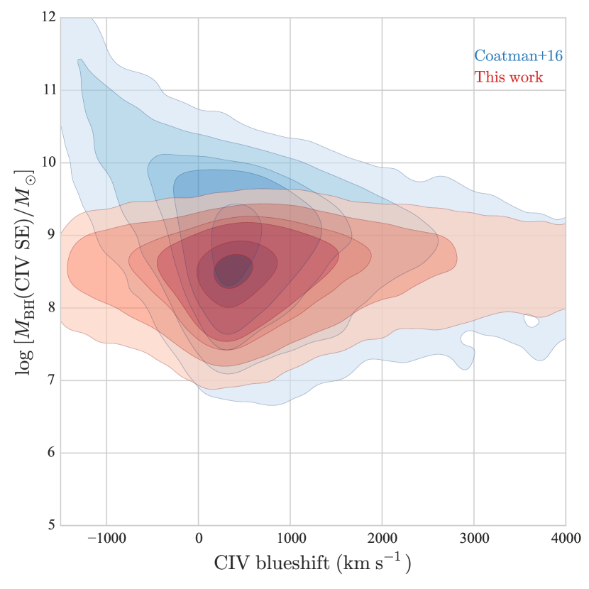
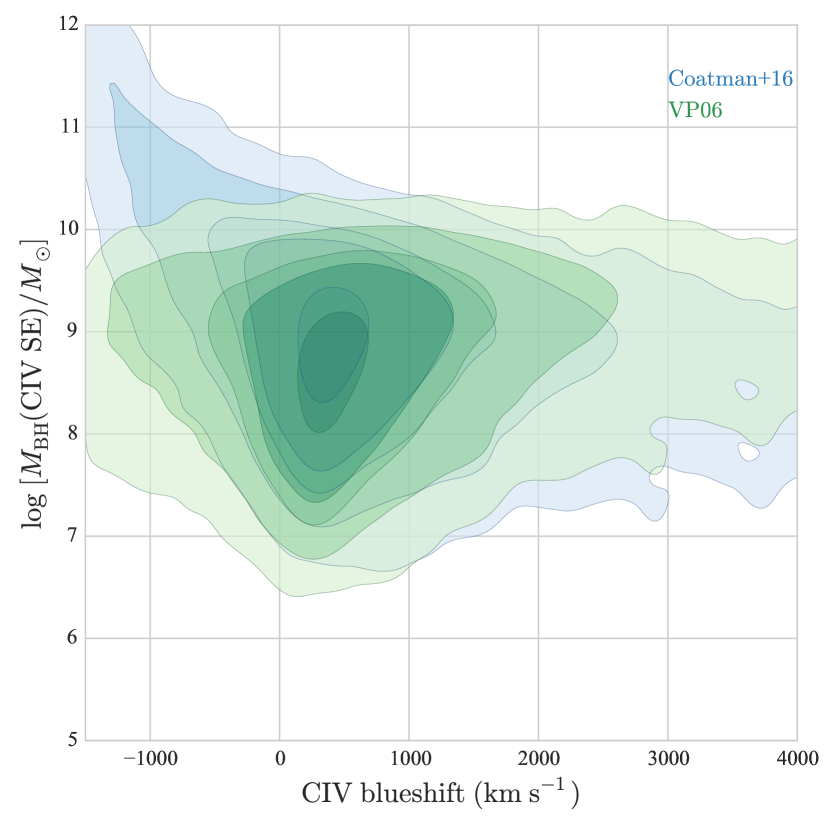
In Figure 11, we compare the overall distributions of C IV FWHM-based BH mass estimates as a function of C IV blueshift using the spectral measurements of DR9 BOSS quasars. The blue shaded contour presents BH masses computed from the blueshift-corrected formula from Coatman et al. (2017), while the red and green shaded contours show those calculated with the new updated recipe in this work and the original VP06 equation, respectively. As can be seen, at large blueshift ($\gtrsim 2000$ km s^-1), our estimator, which does not take into account C IV blueshift, produces a similar mass distribution to the blueshift-corrected distribution. Note that overestimated BH masses from the VP06 estimator are reduced by correcting for the blueshift effect on C IV FWHM (Coatman et al., 2017). Thus, our locally calibrated FWHM-based $M_{\rm BH}$ estimator would be applicable to a sample of high-$z$, high-luminosity quasars having high C IV blueshifts (e.g., $\gtrsim 2000$ km s^-1), giving a consistent mass scale on average.

At the range of small blueshfit ($\sim 0-1000$ km s^-1), where our calibration sample is distributed, the overall mass scale from our estimator is smaller than those of VP06 and Coatman et al. (2017) in the high mass regime ($\gtrsim 10^{8.5}M/M_{\sun}$) and larger in the low mass regime ($\lesssim 10^{8.5}M/M_{\sun}$). This trend has been described in detail by P13. Arguably, our calibration in this work (and P13) has resulted in a better agreement (overall mass scale) with RM masses than that of VP06 in terms of intrinsic scatter and using the higher quality dataset of the updated sample, at least in the mass range ($10^{6.5-9.1}M/M_{\sun}$) where the calibration has been performed. Note that neither our calibration nor that of VP06 (also Coatman et al. 2017, which is based on VP06 calibration) is directly confirmed in the very high-mass BH regime ($\gtrsim 10^{9}M/M_{\sun}$ where most of the Coatman sample is) due to a lack of high-mass RM AGNs in the calibration samples. All these trends are also shown in Fig. 13 of Coatman et al. (2017).

It is also worth noting that striking mass increase toward negative blueshift from using the equation of Coatman et al. (2017) is obviously unreliable, as already discussed by Coatman et al. (2017), due to their insufficient dynamic range of blueshift. This C IV blueshift-corrected recipe should therefore not be used for objects with negative C IV blueshift.

As shown by Coatman et al. (2016), the H$\alpha$ line seems to be also systematically changing as a function of C IV blueshift, although the H$\alpha$ line measurements may not be very accurate due to very low S/N for the H$\alpha$ spectral region (mostly $\lesssim 10$ per resolution element; see their Table 1). If this is true, calibrating SE C IV line to SE H$\alpha$ (or H$\beta$) line as done by Coatman et al. (2016) would be flawed. In other words, correcting C IV FWHM as a function of blueshift against H$\alpha$ FWHM would still be biased since the H$\alpha$ FWHM is also correlated with C IV blueshift. As an ultimate goal, calibrating SE C IV mass estimators against direct C IV RM data (or indirectly against RM Balmer line if C IV RM data is unavailable) for a much larger sample including high-luminosity, high-C IV blueshift AGNs will be the best way to improve the SE mass method. However, given the difficulty of obtaining many direct C IV RM measurements for both low- and high-$z$ AGNs and determining accurate blueshifts (and systemic redshifts) (see, e.g., Denney et al. 2016a; Shen et al. 2016b), our simple calibration of SE C IV-based $M_{\rm BH}$ estimators will still be useful when estimating BH masses from C IV observations of AGNs over a wide range of redshift and luminosity.

4.6. Comparison to other prescriptions

In Figure 12, we compare the H$\beta$-RM based BH masses to the C IV FWHM-based SE BH masses from the corrected prescriptions presented by Denney (2012, their Equation 1) and Runnoe et al. (2013a, their Equation 3). Note that we here use our sample of the local RM AGNs, except for four objects (PG 0026+129, PG 0052+251, PG 1226+023, PG 1307+085) that have not enough spectral coverage to measure the $\lambda 1400$ feature (see Figure 1 of P13). The peak flux of the emission line blend of Si IV$+$O IV] (i.e., $\lambda 1400$ feature) has been measured by fitting it with a local power-law continuum and multi-Gaussian functions following the same method by Runnoe et al. (2013a, see also ). As a direct comparison, we also show the C IV FWHM-based masses using our new calibration (Equation 4).

The SE BH masses using the C IV line shape (FWHM/$\sigma_{\rm line}$) based correction by Denney (2012) shows the overall scatter of $0.39$ dex, which is the same as that of our calibration. However, this corrected prescription is not practically useful because it requires a $\sigma_{\rm line}$ measurement, as well as FWHM, to obtain the shape measurement for the correction to C IV masses. One can use $\sigma_{\rm line}$ directly, if it is available, rather than using FWHM. The slightly larger scatter of $0.43$ dex is observed for the case of the peak flux ratio ($\lambda 1400$/C IV) based correction by Runnoe et al. (2013a). The effect of the correction is less pronounced for our sample, which is not surprising from the investigation by Brotherton et al. (2015), who found that the peak flux ratios measured for the RM AGN sample did not correlated with the difference between H$\beta$ and C IV velocity widths. Our simple calibration is again a useful practical tool in the situation that such additional measurements are not available.

5. SUMMARY AND DISCUSSION

We have updated the calibration of C IV-based SE $M_{\rm BH}$ estimators based on an enlarged AGN sample with high-quality HST UV spectra and using Bayesian linear regression analysis. As an extension of the previous work of P13, there are several improvements over the previous calibration: the sample now covers masses down to $\sim 10^{6.5}M_{\sun}$ with measurements from high-quality and quasi-simultaneous UV-to-optical STIS spectra, and we have used a Bayesian linear regression method to perform outlier-robust inference and take into account covariate distributions and possible correlations between measurement errors.

The results presented in this work are consistent with our previous (P13) and are also in line with Denney (2012) and Denney et al. (2013). We generally recommend use of the $\sigma_{\rm line}$-based or MAD-based C IV $M_{\rm BH}$ estimators, when the measurement are available, since they are better proxies for BLR velocity field (close to the virial relation) and show less scatter in mass estimates than the FWHM-based measurements. Using $\sigma_{\rm line}$ or MAD rather than FWHM for C IV line width measurement is supported by the fact that accurately decomposing and removing a C IV narrow component, if any, is difficult to accomplish with single-epoch spectra. Thus, to avoid possible biases due to a possible C IV core component (Denney, 2012), using the line width measurement that is least affected by uncertain line core (i.e., $\sigma_{\rm line}$ or MAD) appears to be the best approach at present. Measuring $\sigma_{\rm line}$ requires high-quality data to accurately characterize line wings, while MAD is less sensitive to high-velocity wings. C IV-based SE $M_{\rm BH}$ estimators are commonly applied to survey quality data (e.g., SDSS quasars), where $\sigma_{\rm line}$ might not be robustly measured. FWHM is relatively straightforward to measure even in low S/N data, and FWHM measurements are usually provided as the primary measure of line width in survey catalogs (see, e.g., Shen et al. 2011; Pâris et al. 2017). However, this does not mean that C IV FWHM provides an unbiased estimate of the C IV virial velocity in low-quality data. Furthermore, Denney et al. (2013) showed that high-quality data do not improve C IV FWHM-based BH mass estimates, and the best-quality C IV-based BH masses are obtained using $\sigma_{\rm line}$ values measured from high-quality data.

All the calibrations presented in this work and other similar works from literature are, however, subject to sample biases from incompleteness of the calibration samples. Although we were able to expand the BH mass range to lower masses compared with previous work, there is still a lack of calibration objects at very high masses ($\gtrsim 10^{9}M_{\odot}$) and in the regime of strong blueshifts. It is thus important to conduct direct tests of the reliability of extrapolation of this calibration toward high-redshift, high-luminosity quasars, which commonly have high BH mass and/or strong C IV blueshift, as discussed by Richards et al. (2011) and Shen (2013). Current and future multi-object RM programs including SDSS-RM (Shen et al., 2015), OzDES (King et al., 2015), and MSE (McConnachie et al., 2016) will help to improve this situation by providing direct reverberation measurements for rest-frame UV lines in large numbers of quasars. There have been other efforts to improve the calibration of the C IV SE mass scale by taking into account C IV blueshifts (e.g., Shen & Liu 2012; Coatman et al. 2016, 2017) and by making use of other measured quantities including UV-to-optical color, line shape, and nearby line peak flux ratio in the calibration of the SE method (Assef et al. 2011; Denney 2012; Runnoe et al. 2013a; Brotherton et al. 2015). However, the most fundamental and best way of achieving an accurate calibration of C IV-based BH mass estimators will only be from direct C IV reverberation mapping of significant samples of AGN.

A spectrum with broad wavelength coverage observed simultaneously is essential in order to accurately investigate the rest-frame UV-to-optical continuum and emission lines and velocity offsets between them without suffering from systematics due to intrinsic AGN variability (see, e.g., Ho et al. 2012; Capellupo et al. 2015; Mejía-Restrepo et al. 2016 for such datasets). However, even with such data at hand, it is difficult to achieve good continuum fits over the region from $\sim 3100$ Å to $\sim 4000$ Å if fitting the entire spectral region at once, due to the incompleteness and limitation of the currently used AGN Fe II emission templates. No available template covers the full UV/optical range, which is essential to constrain the Balmer continuum and Fe II emission accurately and continuously. There is a need for further improvement in Fe II templates, and an ideal dataset for construction of a new template would consist of complete UV and optical spectra at high S/N, observed with a small spectroscopic aperture to minimize starlight and narrow emission-line components. New HST observations are currently planned that will enable the construction of a new Fe II template using quasi-simultaneous UV and optical STIS data for the nearby Seyfert 1 galaxy Mrk 493 (program GO-14744, PI:Park).

Calibration of Mg II-based SE BH mass estimators using available HST archival spectra as well as our STIS data will be presented in a future paper. As an extension of the work of Wang et al. (2009), our STIS sample will provide an expanded BH mass range to calibrate the Mg II virial relationship and we will provide $\sigma_{\rm line}$ and MAD-based calibrations as well as updated FWHM-based calibrations using the uniform measurement and analysis methods for spectral decompositions, uncertainty estimates, and Bayesian linear regression presented in this work.

Figure 1.— Final fully reduced and combined STIS spectra for our sample of the six low-mass AGNs.

Figure 2.— Multi-component spectral decompositions in the spectral regions of three major broad emission lines, C IV $\lambda 1549$, Mg II $\lambda 2798$, and H$\beta$ $\lambda 4861$, for our 6 AGNs. In each panel, the observed spectrum (black) is decomposed into various components. Left (C IV): the power-law continuum (green), C IV $\lambda 1549$ (magenta), and other nearby blended lines, N IV] $\lambda 1486$ (orange), He II $\lambda 1640$ (blue), O III] $\lambda 1663$ (brown). Middle (Mg II): the power-law continuum (green), Fe II template (orange), Balmer continuum (blue), Mg II $\lambda 2798$ (magenta). Right (H$\beta$): the power-law continuum (green), Fe II template (orange), three narrow emission lines (H$\beta$, [O III] $\lambda\lambda 4959,5007$; blue), broad H$\beta$ (magenta), and the broad and narrow He II $\lambda 4686$ components (brown; only included if blended with H$\beta$). The red line in each panel indicates the full model combining all the best-fit model components. Each bottom gray line represents residual, i.e., data $-$ model, shifted downward for clarity.

Figure 3.— Comparison of the modeled emission line profiles, normalized by each peak, of the C IV (red), Mg II (green), and H$\beta$ (black) for our STIS sample.

Figure 4.— Intercomparison of line width measurements, FWHM and $\sigma_{\rm line}$, of the C IV, Mg II, and H$\beta$ for our STIS sample. The dashed line represents a one-to-one relation in each panel. The dotted line shows the ratio of FWHM to $\sigma_{\rm line}$ for a Gaussian profile. The mean offset (i.e., average of line width differences) and 1$\sigma$ scatter (i.e., standard deviation of line width differences) are given at the lower right corner in each panel.

Figure 5.— Calibration results of C IV-based SE BH mass estimators using FWHM (left) and $\sigma_{\rm line}$ (right). The newly added low-mass AGN sample (6 objects) is indicated with red filled circles while the black filled circles represent the previous archival sample of 25 objects from P13. Blue shaded contours, whose blue (light blue) area corresponds to the 68% (95%) credible region, show posterior predictive distributions under the fitted model as a self-consistency check (see text). The resulting regression parameters with the uncertainty estimates and the overall scatter are given in lower right corner in each panel. Note that the error bars in the y-axis (RM mass) represent the quadratic sum of the propagated RM measurement uncertainty for the virial product (VP) and the adopted uncertainty for the virial factor, and those in the x-axis (SE mass) represent the quadratic sum of the propagated SE calibration uncertainty and the resulting overall scatter.

Figure 6.— Posterior distributions of the resulting parameters of the calibrations in Fig. 5 for the cases of FWHM (left) and $\sigma_{\rm line}$ (right). The red solid line indicates the posterior median estimate, and the black dashed line marks the uncertainty ranges (i.e., 16% and 84% posterior quantiles). The 2D marginal distributions (black) of the parameter pairs are shown on the off-diagonal panels, while the 1D marginalized histogram (blue) for each parameter from the posterior sample is given on the diagonal panels. This figure is made using the corner.py.

Figure 7.— Three-dimensional representation of the calibration results of Fig. 5 for clarification. The red sphere indicates observed data. The colored tilted plane represents the resulting calibration with Equation 2. The black vertical line connecting the data point to the fitted plane shows mass deviation between the observed RM mass and calibrated SE mass.

Figure 8.— Comparison of SE C IV velocity width measurements, FWHM (left) and $\sigma_{\rm line}$ (right), to the observed RM masses.

Figure 9.— Comparisons of the resulting posterior distributions using Stan to those using mlinmix_err (left) and FITEXY (right). The one- and two-dimensional distributions of a parameter (diagonal panels) and parameter pairs (off-diagonal panels) are shown with the kernel density estimate using the GetDist python package. Note that some amount of smoothing has been applied for a clarity of comparison between the distributions.

Figure 10.— Comparison of MAD to FWHM (left) and line dispersion ($\sigma_{\rm line}$; right) measurements for our sample of all 31 AGNs. The dashed line shows a one-to-one relation. The mean offset and 1$\sigma$ scatter are given at the lower right corner.

Figure 11.— Distributions of C IV FWHM-based $M_{\rm BH}$ estimates as a function of C IV blueshift for SDSS quasars from the DR9 BOSS quasar catalog. Most of them are in the redshift range $2\lesssim z\lesssim 3$. The left panel compares BH masses computed from the new calibration of this work (red) to those using the blueshift-corrected recipe from Coatman et al. (2017) (blue) while BH masses using the calibration of VP06 (green) are compared in the right panel. This figure is made using the Seaborn python package.

Figure 12.— Comparisons of C IV FWHM-based SE $M_{\rm BH}$ estimates using our new calibration (top), the C IV line shape based correction by Denney (2012) (middle), and the $\lambda 1400$ feature based correction by Runnoe et al. (2013a) (bottom) to the H$\beta$ RM-based BH masses for our sample of local RM AGNs. The dashed line shows a one-to-one relation, and the 1$\sigma$ scatter is given at the lower right corner in each panel.

Table 1Optical spectral properties from H$\beta$ reverberation mapping

Object	$z$	$\tau_{\rm cent}$	$\sigma_{\rm rms}$	$\log(M_{\rm BH}$/$M_{\odot}$)	References
		(H$\beta$)	(H$\beta$)	(RM)
		(days)	(km s-1)
(1)	(2)	(3)	(4)	(5)	(6)
Sample presented in P13
3C 120	$0.03301$	$27.2^{+1.1}_{-1.1}$	$1514\pm 65$	$7.80\pm 0.31$	6
3C 390.3	$0.05610$	$23.60^{+6.45}_{-6.45}$	$3105\pm 81$	$8.43\pm 0.33$	1
Ark 120	$0.03230$	$39.05^{+4.57}_{-4.57}$	$1896\pm 44$	$8.14\pm 0.32$	1
Fairall 9	$0.04702$	$17.40^{+3.75}_{-3.75}$	$3787\pm 197$	$8.38\pm 0.32$	1
Mrk 279	$0.03045$	$16.70^{+3.90}_{-3.90}$	$1420\pm 96$	$7.51\pm 0.33$	1
Mrk 290	$0.02958$	$8.72^{+1.21}_{-1.02}$	$1609\pm 47$	$7.36\pm 0.32$	4
Mrk 335	$0.02578$	$14.1^{+0.4}_{-0.4}$	$1293\pm 64$	$7.37\pm 0.31$	6
Mrk 509	$0.03440$	$79.60^{+5.75}_{-5.75}$	$1276\pm 28$	$8.12\pm 0.31$	1
Mrk 590	$0.02638$	$24.23^{+2.11}_{-2.11}$	$1653\pm 40$	$7.65\pm 0.32$	1
Mrk 817	$0.03145$	$19.05^{+2.45}_{-2.45}$	$1636\pm 57$	$7.66\pm 0.32$	1
NGC 3516	$0.00884$	$11.68^{+1.02}_{-1.53}$	$1591\pm 10$	$7.47\pm 0.31$	4
NGC 3783	$0.00973$	$10.20^{+2.80}_{-2.80}$	$1753\pm 141$	$7.44\pm 0.32$	1
NGC 4593	$0.00900$	$3.73^{+0.75}_{-0.75}$	$1561\pm 55$	$6.96\pm 0.32$	2
NGC 5548	$0.01717$	$4.18^{+0.86}_{-1.30}$	$3900\pm 266$	$7.80\pm 0.34$	3, 5
NGC 7469	$0.01632$	$4.50^{+0.75}_{-0.75}$	$1456\pm 207$	$7.05\pm 0.31$	1
PG 0026+129	$0.14200$	$111.00^{+26.20}_{-26.20}$	$1773\pm 285$	$8.56\pm 0.33$	1
PG 0052+251	$0.15500$	$89.80^{+24.30}_{-24.30}$	$1783\pm 86$	$8.54\pm 0.32$	1
PG 0804+761	$0.10000$	$146.90^{+18.85}_{-18.85}$	$1971\pm 105$	$8.81\pm 0.31$	1
PG 0953+414	$0.23410$	$150.10^{+22.10}_{-22.10}$	$1306\pm 144$	$8.41\pm 0.32$	1
PG 1226+023	$0.15830$	$306.80^{+79.70}_{-79.70}$	$1777\pm 150$	$8.92\pm 0.32$	1
PG 1229+204	$0.06301$	$37.80^{+21.45}_{-21.45}$	$1385\pm 111$	$7.83\pm 0.38$	1
PG 1307+085	$0.15500$	$105.60^{+41.30}_{-41.30}$	$1820\pm 122$	$8.61\pm 0.33$	1
PG 1426+015	$0.08647$	$95.00^{+33.50}_{-33.50}$	$3442\pm 308$	$9.08\pm 0.34$	1
PG 1613+658	$0.12900$	$40.10^{+15.10}_{-15.10}$	$2547\pm 342$	$8.42\pm 0.38$	1
PG 2130+099	$0.06298$	$12.8^{+1.2}_{-0.9}$	$1825\pm 65$	$7.63\pm 0.31$	6
New sample presented here
Arp 151	$0.02109$	$3.99^{+0.49}_{-0.68}$	$1295\pm 37$	$6.83\pm 0.32$	3, 5
Mrk 1310	$0.01956$	$3.66^{+0.59}_{-0.61}$	$921\pm 135$	$6.50\pm 0.34$	3, 5
Mrk 50	$0.02343$	$10.64^{+0.82}_{-0.93}$	$1740\pm 101$	$7.50\pm 0.32$	7
NGC 6814	$0.00521$	$6.64^{+0.87}_{-0.90}$	$1697\pm 224$	$7.28\pm 0.34$	3, 5
SBS 1116+583A	$0.02787$	$2.31^{+0.62}_{-0.49}$	$1550\pm 310$	$6.74\pm 0.38$	3, 5
Zw 229-015	$0.02788$	$3.86^{+0.69}_{-0.90}$	$1590\pm 47$	$6.99\pm 0.32$	8

Note. — Col. (1) Name. Col. (2) Redshifts are from the NASA/IPAC Extragalactic Database (NED). Col. (3) Rest-frame H$\beta$ time lag measurements. Col. (4) Line dispersion ($\sigma_{\rm line}$) measured from rms spectra. Col. (5) $M_{\rm BH}$ estimates from reverberation mapping: $M_{\rm BH}({\rm RM})=f{\rm VP_{BH}}=fc\tau_{\rm cent}\sigma_{\rm rms}^{2}/G$ where the virial factor $f$ with its uncertainty is adopted from Park et al. 2012a and Woo et al. 2010 (i.e., $\log f=0.71\pm 0.31$). Col. (6) References. 1. Peterson et al. 2004; 2. Denney et al. 2006; 3. Bentz et al. 2009b; 4. Denney et al. 2010; 5. Park et al. 2012b; 6. Grier et al. 2012; 7. Barth et al. 2011b; 8. Barth et al. 2011a

Table 2Summary of HST/STIS observations for the six new AGNs

Object	Observation date	Slit PA	Total exposure time
			G140L	G230L	G430L
		(deg)	(sec)	(sec)	(sec)
Arp 151	2013-04-29	97.7	3801	2639	495
Mrk 1310	2013-06-07	70.8	2624	1255	360
Mrk 50	2012-12-12	-110.8	2624	1255	360
NGC 6814	2013-05-07	-149.6	2848	1299	540
SBS 1116+583A	2013-07-12	28.9	3714	2648	600
Zw 229-015	2013-07-23	117.6	4302	2942	600

Table 3Ultraviolet spectral properties from C IV single-epoch estimates

Object	Telescope/Instrument	Date Observed	S/N	$E(B-V)$	$\log(\lambda L_{\lambda}/$erg s-1$)$	FWHMSE	$\sigma_{\rm SE}$	MADSE	$\rho(W,X)$	$\rho(W,Y)$	$\rho(W,Z)$
			(1450 Å or 1700 Å)		(1350 Å)	(C IV)	(C IV)	(C IV)
			(pix-1)	(mag)		(km s-1)	(km s-1)	(km s-1)
(1)	(2)	(3)	(4)	(5)	(6)	(7)	(8)	(9)	(10)	(11)	(12)
Sample presented in P13
3C 120	IUE/SWP	1994-02-19,27;1994-03-11	$12$	0.263	$44.399\pm 0.021$	$3093\pm 291$	$3106\pm 157$	$2280\pm 74$	$-0.05$	$-0.35$	$-0.50$
3C 390.3	HST/FOS	1996-03-31	$18$	0.063	$43.869\pm 0.003$	$5645\pm 202$	$6154\pm 65$	$4674\pm 42$	$-0.11$	$-0.30$	$-0.32$
Ark 120	HST/FOS	1995-07-29	$17$	0.114	$44.400\pm 0.005$	$3471\pm 108$	$3219\pm 53$	$2345\pm 31$	$0.01$	$-0.30$	$-0.37$
Fairall 9	HST/FOS	1993-01-22	$24$	0.023	$44.442\pm 0.004$	$2649\pm 77$	$2694\pm 20$	$1987\pm 13$	$0.04$	$-0.21$	$-0.17$
Mrk 279	HST/COS	2011-06-27	$9$	0.014	$43.082\pm 0.004$	$4093\pm 388$	$2973\pm 53$	$2202\pm 18$	$0.01$	$-0.04$	$-0.11$
Mrk 290	HST/COS	2009-10-28	$24$	0.014	$43.611\pm 0.002$	$2052\pm 36$	$3531\pm 32$	$2544\pm 14$	$-0.00$	$-0.13$	$-0.20$
Mrk 335	HST/COS	2009-10-31;2010-02-08	$29$	0.032	$43.953\pm 0.001$	$1772\pm 14$	$1876\pm 12$	$1311\pm 7$	$0.03$	$-0.02$	$0.02$
Mrk 509	HST/COS	2009-12-10,11	$107$	0.051	$44.675\pm 0.001$	$3872\pm 18$	$3568\pm 9$	$2601\pm 6$	$0.02$	$-0.07$	$-0.03$
Mrk 590	IUE/SWP	1991-01-14	$17$	0.033	$44.094\pm 0.007$	$5362\pm 266$	$3479\pm 165$	$2630\pm 139$	$-0.09$	$-0.12$	$-0.05$
Mrk 817	HST/COS	2009-08-04;2009-12-28	$38$	0.006	$44.326\pm 0.001$	$4580\pm 48$	$3692\pm 23$	$2756\pm 14$	$-0.01$	$-0.25$	$-0.21$
NGC 3516	HST/COS	2010-10-04;2011-01-22	$20$	0.038	$42.615\pm 0.002$	$2658\pm 34$	$4006\pm 49$	$2864\pm 29$	$-0.03$	$0.07$	$0.06$
NGC 3783	HST/COS	2011-05-26	$29$	0.105	$43.400\pm 0.001$	$2656\pm 444$	$2774\pm 91$	$2014\pm 9$	$-0.01$	$-0.01$	$-0.17$
NGC 4593	HST/STIS	2002-06-23,24	$10$	0.022	$43.761\pm 0.005$	$2952\pm 166$	$2946\pm 162$	$2135\pm 33$	$-0.01$	$-0.00$	$-0.02$
NGC 5548	HST/COS	2011-06-16,17	$36$	0.018	$43.822\pm 0.001$	$1785\pm 82$	$4772\pm 80$	$3528\pm 102$	$0.02$	$-0.11$	$-0.02$
NGC 7469	HST/COS	2010-10-16	$32$	0.061	$43.909\pm 0.001$	$2725\pm 66$	$2849\pm 237$	$2060\pm 15$	$-0.02$	$-0.01$	$-0.14$
PG 0026+129	HST/FOS	1994-11-27	$25$	0.063	$45.236\pm 0.005$	$1604\pm 50$	$4965\pm 113$	$3610\pm 77$	$-0.04$	$-0.11$	$-0.22$
PG 0052+251	HST/FOS	1993-07-22	$21$	0.042	$45.292\pm 0.004$	$5380\pm 87$	$4648\pm 50$	$3463\pm 30$	$-0.12$	$-0.54$	$-0.61$
PG 0804+761	HST/COS	2010-06-12	$34$	0.031	$45.493\pm 0.001$	$3429\pm 23$	$2585\pm 20$	$1932\pm 13$	$0.04$	$0.14$	$0.17$
PG 0953+414	HST/FOS	1991-06-18	$18$	0.012	$45.629\pm 0.005$	$3021\pm 74$	$3448\pm 55$	$2472\pm 35$	$-0.02$	$-0.43$	$-0.48$
PG 1226+023	HST/FOS	1991-01-14,15	$93$	0.018	$46.309\pm 0.001$	$3609\pm 29$	$3513\pm 29$	$2595\pm 19$	$-0.18$	$-0.52$	$-0.60$
PG 1229+204	IUE/SWP	1982-05-01,02	$28$	0.024	$44.609\pm 0.009$	$4023\pm 163$	$2621\pm 90$	$1989\pm 62$	$-0.29$	$-0.48$	$-0.49$
PG 1307+085	HST/FOS	1993-07-21	$14$	0.030	$45.113\pm 0.006$	$3604\pm 111$	$4237\pm 80$	$3010\pm 54$	$-0.13$	$-0.57$	$-0.58$
PG 1426+015	IUE/SWP	1985-03-01,02	$45$	0.028	$45.263\pm 0.004$	$4220\pm 258$	$4808\pm 305$	$3549\pm 95$	$-0.10$	$-0.23$	$-0.42$
PG 1613+658	HST/COS	2010-04-08,09,10	$37$	0.023	$45.488\pm 0.001$	$6398\pm 51$	$4204\pm 17$	$3286\pm 13$	$-0.01$	$-0.10$	$-0.04$
PG 2130+099	HST/COS	2010-10-28	$22$	0.039	$44.447\pm 0.001$	$2147\pm 18$	$2225\pm 47$	$1554\pm 21$	$0.02$	$-0.06$	$-0.07$
New sample presented here
Arp 151	HST/STIS	2013-04-29	$6$	0.012	$41.791\pm 0.017$	$1489\pm 26$	$2900\pm 61$	$1864\pm 35$	$-0.03$	$-0.38$	$-0.46$
Mrk 1310	HST/STIS	2013-06-07	$5$	0.027	$41.715\pm 0.025$	$1434\pm 78$	$2447\pm 108$	$1603\pm 54$	$0.00$	$-0.25$	$-0.31$
Mrk 50	HST/STIS	2012-12-12	$19$	0.015	$43.213\pm 0.003$	$2807\pm 63$	$4443\pm 160$	$3140\pm 115$	$0.02$	$-0.13$	$-0.10$
NGC 6814	HST/STIS	2013-05-07	$6$	0.164	$41.105\pm 0.021$	$2651\pm 264$	$2804\pm 103$	$2096\pm 59$	$0.02$	$-0.07$	$-0.11$
SBS 1116+583A	HST/STIS	2013-07-12	$13$	0.010	$42.867\pm 0.005$	$3253\pm 302$	$3315\pm 231$	$2302\pm 121$	$-0.04$	$-0.13$	$-0.15$
Zw 229-015	HST/STIS	2013-07-23	$17$	0.064	$43.129\pm 0.007$	$2573\pm 71$	$2608\pm 56$	$1891\pm 33$	$-0.05$	$-0.20$	$-0.18$

Note. — Col. (1) Name. Col. (2) Telescope/Instrument from which archival UV spectra were obtained. Note that the new COS spectra were obtained after 2009. Col. (3) Observation date for combined spectra. Col. (4) Signal-to-noise ratio per pixel at 1450 Å or 1700 Å in rest-frame. Col. (5) $E(B-V)$ are from the NASA/IPAC Extragalactic Database (NED) based on the recalibration of Schlafly & Finkbeiner (2011). Col. (6) Continuum luminosity measured at 1350 Å. Col. (7) FWHM measured from SE spectra. Col. (8) Line dispersion ($\sigma_{\rm line}$) measured from SE spectra. Col. (9) MAD (mean absolute deviation around weighted median) measured from SE spectra. Col. (10) correlation coefficient between measurement errors of $W$ and $X$ where $W=\log\lambda L_{\lambda}$ at 1350 Å and $X=\log\rm FWHM_{\rm SE}$. Col. (11) correlation coefficient between measurement errors of $W$ and $Y$ where $Y=\log\sigma_{\rm SE}$. Col. (12) correlation coefficient between measurement errors of $W$ and $Z$ where $Z=\log\rm MAD_{\rm SE}$.

Table 4C IV $M_{\rm BH}$ estimator calibration results
$\log[M_{\rm BH}{\rm(RM)}/M_{\odot}]=~{}\alpha~{}+~{}\beta~{}\log(L_{1350\textrm{\AA}}/10^{44}~{}\rm erg~{}s^{-1})~{}+~{}\gamma~{}\log[\varDelta V(\textrm{{C~{}IV}})/1000~{}\rm km~{}s^{-1}]$

$\varDelta V(\textrm{{C~{}IV}})$	$\alpha$	$\beta$	$\gamma$	$\sigma_{{\mathop{\rm int}}}$	mean offset	1$\sigma$ scatter	Ref.
					(dex)	(dex)
Previous calibrations
$\sigma_{\rm line}$	$6.73\pm 0.01$	$0.53$	$2$	$0.33$	$\cdots$	$\cdots$	VP06
FWHM	$6.66\pm 0.01$	$0.53$	$2$	$0.36$	$\cdots$	$\cdots$	VP06
$\sigma_{\rm line}$	$6.71\pm 0.07$	$0.50\pm 0.07$	$2$	$0.28\pm 0.04$	$0.00$	$0.295$	P13
FWHM	$7.48\pm 0.24$	$0.52\pm 0.09$	$0.56\pm 0.48$	$0.35\pm 0.05$	$0.00$	$0.347$	P13
This work
$\sigma_{\rm line}$	$6.90^{+0.35}_{-0.34}$	$0.44^{+0.07}_{-0.07}$	$1.66^{+0.65}_{-0.66}$	$0.12^{+0.09}_{-0.06}$	$0.01$	$0.33$
FWHM	${\bf 7.54}^{+0.26}_{-0.27}$	${\bf 0.45}^{+0.08}_{-0.08}$	${\bf 0.50}^{+0.55}_{-0.53}$	$0.16^{+0.10}_{-0.08}$	$0.00$	$0.37$	best-fit
MAD	$7.15^{+0.24}_{-0.25}$	$0.42^{+0.07}_{-0.07}$	$1.65^{+0.61}_{-0.62}$	$0.12^{+0.09}_{-0.06}$	$0.00$	$0.33$
This work (fixing $\gamma=2$)
$\sigma_{\rm line}$	${\bf 6.73}^{+0.07}_{-0.07}$	${\bf 0.43}^{+0.06}_{-0.06}$	${\bf 2}$	$0.12^{+0.09}_{-0.06}$	$0.01$	$0.33$	best-fit
FWHM	$6.84^{+0.09}_{-0.09}$	$0.33^{+0.07}_{-0.07}$	$2$	$0.22^{+0.11}_{-0.10}$	$-0.01$	$0.43$
MAD	${\bf 7.01}^{+0.07}_{-0.07}$	${\bf 0.41}^{+0.06}_{-0.06}$	${\bf 2}$	$0.12^{+0.09}_{-0.06}$	$0.00$	$0.33$	best-fit
This work (fixing $\beta=0.5$)
$\sigma_{\rm line}$	$6.99^{+0.34}_{-0.34}$	$0.5$	$1.49^{+0.63}_{-0.62}$	$0.12^{+0.09}_{-0.06}$	$0.01$	$0.34$
FWHM	$7.62^{+0.23}_{-0.23}$	$0.5$	$0.31^{+0.46}_{-0.45}$	$0.16^{+0.10}_{-0.08}$	$0.01$	$0.38$
MAD	$7.23^{+0.24}_{-0.24}$	$0.5$	$1.41^{+0.57}_{-0.58}$	$0.12^{+0.09}_{-0.06}$	$0.01$	$0.34$
This work (fixing $\beta=0.5$ and $\gamma=2$)
$\sigma_{\rm line}$	$6.72^{+0.07}_{-0.07}$	$0.5$	$2$	$0.12^{+0.08}_{-0.06}$	$0.01$	$0.35$
FWHM	$6.82^{+0.09}_{-0.09}$	$0.5$	$2$	$0.26^{+0.11}_{-0.11}$	$0.00$	$0.47$
MAD	$7.00^{+0.07}_{-0.07}$	$0.5$	$2$	$0.12^{+0.09}_{-0.06}$	$0.01$	$0.35$

Note. — The mean offset and $1\sigma$ scatter for our calibrations are measured from the average and standard deviation of mass residuals between RM masses and calibrated SE masses, $\varDelta=\log M_{\rm BH}{\rm(RM)}-\log M_{\rm BH}{\rm(SE)}$. Note that the apparent big difference in $\sigma_{\rm int}$ estimates between the previous calibrations and this work is mostly due to the differences in the adopted RM mass error and statitcal model. The uncertainty of $\log f$ (i.e., 0.31 dex) is added in quadrature to the uncertainties of RM BH masses in this work. The standard deviation ($\sigma$) of the $t$ distribution is by definition different (larger) from that of Gaussian distribution due to the heavy-tail when the degrees-of-freedom parameter is small. In this case, the $\sigma_{\rm int}$ parameter of the $t$ distribution model is not the same as the data sperad ($\sigma$) of the $t$ distribution.

Table 5Comparing calibration results with other linear regression methods

Method	$\alpha$	$\beta$	$\gamma$	$\sigma_{{\mathop{\rm int}}}$	mean offset	1$\sigma$ scatter
					(dex)	(dex)
Stan (Bayesian)	$7.54_{-0.27}^{+0.26}$	$0.45_{-0.08}^{+0.08}$	$0.50_{-0.53}^{+0.55}$	$0.16_{-0.08}^{+0.10}$	$0.00$	$0.37$
mlinmix_err (Bayesian)	$7.51_{-0.25}^{+0.25}$	$0.43_{-0.07}^{+0.07}$	$0.57_{-0.51}^{+0.50}$	$0.24_{-0.09}^{+0.09}$	$-0.00$	$0.37$
FITEXY ($\chi^{2}$-based)	$7.50\pm 0.22$	$0.43\pm 0.08$	$0.59\pm 0.46$	$0.20\pm 0.10$	$-0.00$	$0.37$

Note. — For a consistent comparison, the exactly same methodology of FITEXY used by P13 is applied.

References

- Assef et al. (2012) Assef, R. J., Frank, S., Grier, C. J., et al. 2012, ApJ, 753, L2
- Assef et al. (2011) Assef, R. J., Denney, K. D., Kochanek, C. S., et al. 2011, ApJ, 742, 93
- Barnard et al. (2000) Barnard, J., McCulloch, R., & Meng, X.-L. 2000, Statistica Sinica, 10, 1281
- Barth et al. (2011a) Barth, A. J., Nguyen, M. L., Malkan, M. A., et al. 2011a, ApJ, 732, 121
- Barth et al. (2011b) Barth, A. J., Pancoast, A., Thorman, S. J., et al. 2011b, ApJ, 743, L4
- Barth et al. (2013) Barth, A. J., Pancoast, A., Bennert, V. N., et al. 2013, ApJ, 769, 128
- Barth et al. (2015) Barth, A. J., Bennert, V. N., Canalizo, G., et al. 2015, ApJS, 217, 26
- Bennert et al. (2015) Bennert, V. N., Treu, T., Auger, M. W., et al. 2015, ApJ, 809, 20
- Bentz (2016) Bentz, M. C. 2016, in Astrophysics and Space Science Library, Vol. 439, Astrophysics and Space Science Library, ed. H. M. J. Boffin, G. Hussain, J.-P. Berger, & L. Schmidtobreick, 249
- Bentz et al. (2009a) Bentz, M. C., Peterson, B. M., Netzer, H., Pogge, R. W., & Vestergaard, M. 2009a, ApJ, 697, 160
- Bentz et al. (2006) Bentz, M. C., Peterson, B. M., Pogge, R. W., Vestergaard, M., & Onken, C. A. 2006, ApJ, 644, 133
- Bentz et al. (2009b) Bentz, M. C., Walsh, J. L., Barth, A. J., et al. 2009b, ApJ, 705, 199
- Bentz et al. (2013) Bentz, M. C., Denney, K. D., Grier, C. J., et al. 2013, ApJ, 767, 149
- Betancourt & Girolami (2013) Betancourt, M. J., & Girolami, M. 2013, ArXiv e-prints, arXiv:1312.0906
- Boroson & Green (1992) Boroson, T. A., & Green, R. F. 1992, ApJS, 80, 109
- Brotherton et al. (2015) Brotherton, M. S., Runnoe, J. C., Shang, Z., & DiPompeo, M. A. 2015, MNRAS, 451, 1290
- Brotherton et al. (1994) Brotherton, M. S., Wills, B. J., Steidel, C. C., & Sargent, W. L. W. 1994, ApJ, 423, 131
- Bruhweiler & Verner (2008) Bruhweiler, F., & Verner, E. 2008, ApJ, 675, 83
- Capellupo et al. (2015) Capellupo, D. M., Netzer, H., Lira, P., Trakhtenbrot, B., & Mejía-Restrepo, J. 2015, MNRAS, 446, 3427
- Cappellari et al. (2002) Cappellari, M., Verolme, E. K., van der Marel, R. P., et al. 2002, ApJ, 578, 787
- Chevallard & Charlot (2016) Chevallard, J., & Charlot, S. 2016, MNRAS, 462, 1415
- Coatman et al. (2016) Coatman, L., Hewett, P. C., Banerji, M., & Richards, G. T. 2016, MNRAS, 461, 647
- Coatman et al. (2017) Coatman, L., Hewett, P. C., Banerji, M., et al. 2017, MNRAS, 465, 2120
- Croom (2011) Croom, S. M. 2011, ApJ, 736, 161
- De Rosa et al. (2011) De Rosa, G., Decarli, R., Walter, F., et al. 2011, ApJ, 739, 56
- De Rosa et al. (2014) De Rosa, G., Venemans, B. P., Decarli, R., et al. 2014, ApJ, 790, 145
- Denney (2012) Denney, K. D. 2012, ApJ, 759, 44
- Denney et al. (2016a) Denney, K. D., Horne, K., Brandt, W. N., et al. 2016a, ApJ, 833, 33
- Denney et al. (2013) Denney, K. D., Pogge, R. W., Assef, R. J., et al. 2013, ApJ, 775, 60
- Denney et al. (2006) Denney, K. D., Bentz, M. C., Peterson, B. M., et al. 2006, ApJ, 653, 152
- Denney et al. (2010) Denney, K. D., Peterson, B. M., Pogge, R. W., et al. 2010, ApJ, 721, 715
- Denney et al. (2016b) Denney, K. D., Horne, K., Shen, Y., et al. 2016b, ApJS, 224, 14
- Dietrich et al. (2002) Dietrich, M., Appenzeller, I., Vestergaard, M., & Wagner, S. J. 2002, ApJ, 564, 581
- Dietrich et al. (2003) Dietrich, M., Hamann, F., Appenzeller, I., & Vestergaard, M. 2003, ApJ, 596, 817
- Ferrarese & Ford (2005) Ferrarese, L., & Ford, H. 2005, Space Sci. Rev., 116, 523
- Fine et al. (2010) Fine, S., Croom, S. M., Bland-Hawthorn, J., et al. 2010, MNRAS, 409, 591
- Fitzpatrick (1999) Fitzpatrick, E. L. 1999, PASP, 111, 63
- Gelman et al. (2013) Gelman, A., Carlin, J., Stern, H., et al. 2013, Bayesian Data Analysis, Third Edition, Chapman & Hall/CRC Texts in Statistical Science (Taylor & Francis)
- Grandi (1982) Grandi, S. A. 1982, ApJ, 255, 25
- Greene et al. (2010) Greene, J. E., Peng, C. Y., & Ludwig, R. R. 2010, ApJ, 709, 937
- Grier et al. (2012) Grier, C. J., Peterson, B. M., Pogge, R. W., et al. 2012, ApJ, 755, 60
- Ho et al. (2012) Ho, L. C., Goldoni, P., Dong, X.-B., Greene, J. E., & Ponti, G. 2012, ApJ, 754, 11
- Hoffman & Gelman (2014) Hoffman, M. D., & Gelman, A. 2014, Journal of Machine Learning Research, 15, 1593
- Hogg et al. (2010) Hogg, D. W., Bovy, J., & Lang, D. 2010, ArXiv e-prints, arXiv:1008.4686
- Kaspi et al. (2007) Kaspi, S., Brandt, W. N., Maoz, D., et al. 2007, ApJ, 659, 997
- Kaspi et al. (2005) Kaspi, S., Maoz, D., Netzer, H., et al. 2005, ApJ, 629, 61
- Kaspi et al. (2000) Kaspi, S., Smith, P. S., Netzer, H., et al. 2000, ApJ, 533, 631
- Kelly (2007) Kelly, B. C. 2007, ApJ, 665, 1489
- Kelly (2011) —. 2011, ArXiv e-prints, arXiv:1112.1745
- Kelly et al. (2012) Kelly, B. C., Shetty, R., Stutz, A. M., et al. 2012, ApJ, 752, 55
- King et al. (2015) King, A. L., Martini, P., Davis, T. M., et al. 2015, MNRAS, 453, 1701
- Kokubo et al. (2014) Kokubo, M., Morokuma, T., Minezaki, T., et al. 2014, ApJ, 783, 46
- Kollatschny (2003) Kollatschny, W. 2003, A&A, 407, 461
- Kormendy & Ho (2013) Kormendy, J., & Ho, L. C. 2013, ARA&A, 51, 511
- Kovačević et al. (2010) Kovačević, J., Popović, L. Č., & Dimitrijević, M. S. 2010, ApJS, 189, 15
- Kovačević et al. (2014) Kovačević, J., Popović, L. Č., & Kollatschny, W. 2014, Advances in Space Research, 54, 1347
- Kruschke (2014) Kruschke, J. 2014, Doing Bayesian Data Analysis: A Tutorial with R, JAGS, and Stan, 2nd edn. (Elsevier Science)
- Kurk et al. (2007) Kurk, J. D., Walter, F., Fan, X., et al. 2007, ApJ, 669, 32
- Malkan & Sargent (1982) Malkan, M. A., & Sargent, W. L. W. 1982, ApJ, 254, 22
- Markwardt (2009) Markwardt, C. B. 2009, in Astronomical Society of the Pacific Conference Series, Vol. 411, Astronomical Data Analysis Software and Systems XVIII, ed. D. A. Bohlender, D. Durand, & P. Dowler, 251
- McConnachie et al. (2016) McConnachie, A., Babusiaux, C., Balogh, M., et al. 2016, ArXiv e-prints, arXiv:1606.00043
- McLure & Jarvis (2002) McLure, R. J., & Jarvis, M. J. 2002, MNRAS, 337, 109
- Mejía-Restrepo et al. (2016) Mejía-Restrepo, J. E., Trakhtenbrot, B., Lira, P., Netzer, H., & Capellupo, D. M. 2016, MNRAS, 460, 187
- Neal (2012) Neal, R. M. 2012, ArXiv e-prints, arXiv:1206.1901
- Nobuta et al. (2012) Nobuta, K., Akiyama, M., Ueda, Y., et al. 2012, ApJ, 761, 143
- Pancoast et al. (2014) Pancoast, A., Brewer, B. J., Treu, T., et al. 2014, MNRAS, 445, 3073
- Pancoast et al. (2012) —. 2012, ApJ, 754, 49
- Pâris et al. (2017) Pâris, I., Petitjean, P., Ross, N. P., et al. 2017, A&A, 597, A79
- Park et al. (2012a) Park, D., Kelly, B. C., Woo, J.-H., & Treu, T. 2012a, ApJS, 203, 6
- Park et al. (2015) Park, D., Woo, J.-H., Bennert, V. N., et al. 2015, ApJ, 799, 164
- Park et al. (2013) Park, D., Woo, J.-H., Denney, K. D., & Shin, J. 2013, ApJ, 770, 87
- Park et al. (2012b) Park, D., Woo, J.-H., Treu, T., et al. 2012b, ApJ, 747, 30
- Peterson & Wandel (1999) Peterson, B. M., & Wandel, A. 1999, ApJ, 521, L95
- Peterson et al. (2004) Peterson, B. M., Ferrarese, L., Gilbert, K. M., et al. 2004, ApJ, 613, 682
- Richards et al. (2002) Richards, G. T., Vanden Berk, D. E., Reichard, T. A., et al. 2002, AJ, 124, 1
- Richards et al. (2011) Richards, G. T., Kruczek, N. E., Gallagher, S. C., et al. 2011, AJ, 141, 167
- Runco et al. (2016) Runco, J. N., Cosens, M., Bennert, V. N., et al. 2016, ApJ, 821, 33
- Runnoe et al. (2014) Runnoe, J. C., Brotherton, M. S., DiPompeo, M. A., & Shang, Z. 2014, MNRAS, 438, 3263
- Runnoe et al. (2013a) Runnoe, J. C., Brotherton, M. S., Shang, Z., & DiPompeo, M. A. 2013a, MNRAS, 434, 848
- Runnoe et al. (2013b) Runnoe, J. C., Brotherton, M. S., Shang, Z., Wills, B. J., & DiPompeo, M. A. 2013b, MNRAS, 429, 135
- Savaglio et al. (2004) Savaglio, S., Glazebrook, K., Abraham, R. G., et al. 2004, ApJ, 602, 51
- Schlafly & Finkbeiner (2011) Schlafly, E. F., & Finkbeiner, D. P. 2011, ApJ, 737, 103
- Shang et al. (2007) Shang, Z., Wills, B. J., Wills, D., & Brotherton, M. S. 2007, AJ, 134, 294
- Shen (2013) Shen, Y. 2013, Bulletin of the Astronomical Society of India, 41, 61
- Shen et al. (2008) Shen, Y., Greene, J. E., Strauss, M. A., Richards, G. T., & Schneider, D. P. 2008, ApJ, 680, 169
- Shen & Ho (2014) Shen, Y., & Ho, L. C. 2014, Nature, 513, 210
- Shen & Liu (2012) Shen, Y., & Liu, X. 2012, ApJ, 753, 125
- Shen et al. (2011) Shen, Y., Richards, G. T., Strauss, M. A., et al. 2011, ApJS, 194, 45
- Shen et al. (2015) Shen, Y., Brandt, W. N., Dawson, K. S., et al. 2015, ApJS, 216, 4
- Shen et al. (2016a) Shen, Y., Horne, K., Grier, C. J., et al. 2016a, ApJ, 818, 30
- Shen et al. (2016b) Shen, Y., Brandt, W. N., Richards, G. T., et al. 2016b, ApJ, 831, 7
- Stan Development Team (2015a) Stan Development Team. 2015a, Stan: A C++ Library for Probability and Sampling, Version 2.9.0
- Stan Development Team (2015b) —. 2015b, Stan Modeling Language Users Guide and Reference Manual, Version 2.9.0
- Stan Development Team (2016) —. 2016, PyStan: the Python interface to Stan, Version 2.9.0
- Storey & Hummer (1995) Storey, P. J., & Hummer, D. G. 1995, MNRAS, 272, 41
- Tremaine et al. (2002) Tremaine, S., Gebhardt, K., Bender, R., et al. 2002, ApJ, 574, 740
- Trevese et al. (2014) Trevese, D., Perna, M., Vagnetti, F., Saturni, F. G., & Dadina, M. 2014, ApJ, 795, 164
- Tsuzuki et al. (2006) Tsuzuki, Y., Kawara, K., Yoshii, Y., et al. 2006, ApJ, 650, 57
- van der Marel & Franx (1993) van der Marel, R. P., & Franx, M. 1993, ApJ, 407, 525
- van Dokkum (2001) van Dokkum, P. G. 2001, PASP, 113, 1420
- Véron-Cetty et al. (2004) Véron-Cetty, M.-P., Joly, M., & Véron, P. 2004, A&A, 417, 515
- Vestergaard & Peterson (2006) Vestergaard, M., & Peterson, B. M. 2006, ApJ, 641, 689
- Vestergaard & Wilkes (2001) Vestergaard, M., & Wilkes, B. J. 2001, ApJS, 134, 1
- Walsh et al. (2013) Walsh, J. L., Barth, A. J., Ho, L. C., & Sarzi, M. 2013, ApJ, 770, 86
- Wang et al. (2009) Wang, J.-G., Dong, X.-B., Wang, T.-G., et al. 2009, ApJ, 707, 1334
- Wills et al. (1993) Wills, B. J., Brotherton, M. S., Fang, D., Steidel, C. C., & Sargent, W. L. W. 1993, ApJ, 415, 563
- Wills et al. (1985) Wills, B. J., Netzer, H., & Wills, D. 1985, ApJ, 288, 94
- Woo et al. (2013) Woo, J.-H., Schulze, A., Park, D., et al. 2013, ApJ, 772, 49
- Woo et al. (2006) Woo, J.-H., Treu, T., Malkan, M. A., & Blandford, R. D. 2006, ApJ, 645, 900
- Woo et al. (2015) Woo, J.-H., Yoon, Y., Park, S., Park, D., & Kim, S. C. 2015, ApJ, 801, 38
- Woo et al. (2010) Woo, J.-H., Treu, T., Barth, A. J., et al. 2010, ApJ, 716, 269