$B_{s}\rightarrow D_{s}\;\ell\,\nu$ Form Factors and the Fragmentation Fraction Ratio $f_{s}/f_{d}$

Abstract

We present a lattice quantum chromodynamics determination of the scalar and vector form factors for the $B_{s}\rightarrow D_{s}\ell\nu$ decay over the full physical range of momentum transfer. In conjunction with future experimental data, our results will provide a new method to extract $|V_{cb}|$, which may elucidate the current tension between exclusive and inclusive determinations of this parameter. Combining the form factor results at non-zero recoil with recent HPQCD results for the $B\rightarrow D\ell\nu$ form factors, we determine the ratios $f^{B_{s}\rightarrow D_{s}}_{0}(M_{\pi}^{2})/f^{B\rightarrow D}_{0}(M_{K}^{2})=1.000(62)$ and $f^{B_{s}\rightarrow D_{s}}_{0}(M_{\pi}^{2})/f^{B\rightarrow D}_{0}(M_{\pi}^{2})=1.006(62)$. These results give the fragmentation fraction ratios $f_{s}/f_{d}=0.310(30)_{\mathrm{stat.}}(21)_{\mathrm{syst.}}(6)_{\mathrm{theor.}}(38)_{\mathrm{latt.}}$ and $f_{s}/f_{d}=0.307(16)_{\mathrm{stat.}}(21)_{\mathrm{syst.}}(23)_{\mathrm{theor.}}(44)_{\mathrm{latt.}}$, respectively. The fragmentation fraction ratio is an important ingredient in experimental determinations of $B_{s}$ meson branching fractions at hadron colliders, in particular for the rare decay ${\cal B}(B_{s}\rightarrow\mu^{+}\mu^{-})$. In addition to the form factor results, we make the first prediction of the branching fraction ratio $R(D_{s})={\cal B}(B_{s}\to D_{s}\tau\nu)/{\cal B}(B_{s}\to D_{s}\ell\nu)=0.301(6)$, where $\ell$ is an electron or muon. Current experimental measurements of the corresponding ratio for the semileptonic decays of $B$ mesons disagree with Standard Model expectations at the level of nearly four standard deviations. Future experimental measurements of $R(D_{s})$ may help understand this discrepancy.

I Introduction

Studies of $B$ and $B_{s}$ meson decays at the Large Hadron Collider provide precision tests of the Standard Model of particle physics and are an important tool in the search for new physics. For example, the first observation of the rare decay $B_{s}\rightarrow\mu^{+}\mu^{-}$, through a combined analysis by the LHCb and CMS collaborations Khachatryan et al. (2015); Aaij et al. (2017), tested the Standard Model prediction of the branching fraction. This decay is doubly-suppressed in the Standard Model, but may have large contributions from physics beyond the Standard Model (see, for example, Ge et al. (2016)). Although the observed branching fraction is currently consistent with Standard Model expectations, there is still considerable room for new physics, given the experimental and theoretical uncertainties. Both LHCb and CMS are expected to reduce their errors significantly in Run II and tightening constraints on possible new physics requires a corresponding improvement in the theoretical determination of the Standard Model branching fraction.

Extraction of the $B_{s}$ meson branching fraction ${\cal B}(B_{s}\rightarrow\mu^{+}\mu^{-})$ relies on the normalization channels $B^{+}_{u}\rightarrow J/\Psi(\mu^{+}\mu^{-})K^{+}$ and $B^{0}_{d}\rightarrow K^{+}\pi_{-}$ Adeva et al. (2009). The branching fraction can then be expressed as Khachatryan et al. (2015)

$${\cal B}(B_{s}\rightarrow\mu^{+}\mu^{-})={\cal B}(B_{q}\rightarrow X)\frac{f_{q}}{f_{s}}\frac{\epsilon_{X}}{\epsilon_{\mu\mu}}\frac{N_{\mu\mu}}{N_{X}},$$ (1)

where the $f_{q}$ are the fragmentation fractions, which give the probability that a $b$-quark hadronizes into a $B_{q}$ meson. The $\epsilon$ factors in this equation represent detector efficiencies and the $N$ factors denote the observed numbers of events.

The analysis of Khachatryan et al. (2015) used the value of $f_{s}/f_{d}=0.259(15)$, determined from LHCb experimental data Aaij et al. (2012, 2013); Storaci et al. (2013). The ratio $f_{s}/f_{d}$ depends on the kinematic range of the experiment, leading to the introduction of an additional systematic uncertainty in the value of $f_{s}/f_{d}$ to account for the extrapolation of the LHCb result to the CMS acceptance. Reducing sources of systematic uncertainties in the value of this ratio will improve the precision of the determination of the $B_{s}\rightarrow\mu^{+}\mu^{-}$ branching fraction. Indeed, an accurate value for the fragmentation fraction ratio is necessary for improved measurements of other $B_{s}$ meson decay branching fractions at the LHC Adeva et al. (2009).

The ratio of the fragmentation fractions, $f_{s}/f_{d}$, can be expressed in terms of the ratios of form factors Fleischer et al. (2010, 2011),

$${\cal N}_{F}=\left[\frac{f_{0}^{(s)}(M_{\pi}^{2})}{f_{0}^{(d)}(M_{K}^{2})}\right]^{2}\quad\mathrm{and}\quad{\cal N}^{\prime}_{F}=\left[\frac{f_{0}^{(s)}(M_{\pi}^{2})}{f_{0}^{(d)}(M_{\pi}^{2})}\right]^{2},$$ (2)

where $f_{0}^{(q)}(M^{2})$ is the scalar form factor of the $B_{q}\rightarrow D_{q}l\nu$ semileptonic decay at $q^{2}=M^{2}$. The first lattice calculations of the form factor ratios in Equation (2) using heavy clover bottom and charm quarks were published in Bailey et al. (2012). In addition, the form factors, $f_{+}(q^{2})$ and $f_{0}(q^{2})$, for the semileptonic decay $B_{s}\rightarrow D_{s}\ell\nu$ were determined with twisted mass fermions for the region near zero recoil in Atoui et al. (2014).

In this article we calculate the form factors, $f_{+}(q^{2})$ and $f_{0}(q^{2})$, for the semileptonic decay $B_{s}\rightarrow D_{s}\ell\nu$. We present a determination of these form factors over the full physical range of momentum transfer, $q^{2}$ using the modified $z$-expansion for the chiral-continuum-kinematic extrapolation. We combine these form factor results with recent HPQCD results for the $B\rightarrow D\ell\nu$ decay Na et al. (2015) to determine the ratios of $B_{s}\rightarrow D_{s}\ell\nu$ and $B\rightarrow D\ell\nu$ form factors relevant to the ratio of fragmentation fractions, $f_{s}/f_{d}$.

We use the non-relativistic (NRQCD) action for the bottom quarks and the Highly Improved Staggered Quark (HISQ) action for the charm quarks. Our form factors for $B\rightarrow D\ell\nu$ have appeared already in Na et al. (2015). Here we first present $B_{s}\rightarrow D_{s}\ell\nu$ form factor results and then proceed to the form factor ratios. We find

$$\frac{f_{0}^{(s)}(M_{\pi}^{2})}{f_{0}^{(d)}(M_{K}^{2})}=1.000(62)\quad{\rm and}\quad\frac{f_{0}^{(s)}(M_{\pi}^{2})}{f_{0}^{(d)}(M_{\pi}^{2})}=1.006(62).$$ (3)

This leads to

$$\frac{f_{s}}{f_{d}}=0.310(30)_{\mathrm{stat.}}(21)_{\mathrm{syst.}}(6)_{\mathrm{theor.}}(38)_{\mathrm{latt.}}$$ (4)

and

$$\frac{f_{s}}{f_{d}}=0.307(16)_{\mathrm{stat.}}(21)_{\mathrm{syst.}}(23)_{\mathrm{theor.}}(44)_{\mathrm{latt.}},$$ (5)

respectively. The uncertainties in these results are: the experimental statistical and systematic uncertainties; theoretical uncertainties (predominantly arising from a factor that captures deviations from naive factorization and, in Equation (5), an electroweak correction factor); and the uncertainties in our lattice input. In quoting these results, we have assumed that there are no correlations between the lattice results and the other sources of uncertainty.

In addition to determining the fragmentation fraction ratio relevant to the measurement of the branching fraction for the rare decay, $B_{s}\rightarrow\mu^{+}\mu^{-}$, the semileptonic $B_{s}\to D_{s}\ell\nu$ decay provides a new method to determine the CKM matrix element $|V_{cb}|$. There is a long-standing tension between determinations of $|V_{cb}|$ from exclusive and inclusive measurements of the semileptonic $B$ meson decays (see, for example, Amhis et al. (2014, 2016a) and the review in Patrigiani et al. (2016)), although recent analyses suggest the tension has eased Gambino et al. (2016); Bigi and Gambino (2016). The $B_{s}\to D_{s}\ell\nu$ decay has yet to be observed experimentally and consequently has received less theoretical attention than semileptonic decays of the $B$ meson. The studies that have been undertaken for the $B_{s}\to D_{s}\ell\nu$ decay include calculations based on relativistic quark models Zhao et al. (2007); Bhol (2014), light-cone sum rules Li et al. (2009), perturbative factorization Fan et al. (2014) and estimates using the Bethe-Salpeter method Li et al. (2010); Chen et al. (2012). At present, there is one unquenched lattice calculation of the form factor ${\cal G}(1)$ at zero recoil Atoui et al. (2014). The FNAL/MILC collaboration has previously studied the ratio of the form factors of the $B_{s}\to D_{s}\ell\nu$ and $B\to D\ell\nu$ decays Bailey et al. (2012).

We determine the form factor for the $B_{s}\to D_{s}\ell\nu$ semileptonic decay at zero momentum transfer to be $f_{0}(0)=f_{+}(0)=0.656(31)$ and at zero recoil to be ${\cal G}(1)\propto f_{+}(q^{2}_{\mathrm{max}})=1.068(40)$. Although experimental data is frequently presented in the form $|V_{cb}|{\cal G}(1)$, the additional information provided by our calculation of the shape of the form factors throughout the kinematic range will, when combined with future experimental data, provide a new method to extract $|V_{cb}|$ and may elucidate the puzzle of the tension between inclusive and exclusive determinations of this CKM matrix element.

In the next section we briefly outline the details of the calculation, including the gauge ensembles, bottom-charm currents and two- and three-point correlator construction. Our calculation closely parallels that presented in Na et al. (2015) for the $B\rightarrow D\ell\nu$ semileptonic decay and we refer the reader to that work for further details. In Section III we discuss correlator fits to our lattice data and Section IV covers the chiral-continuum-kinematic extrapolations, which follows closely the methodology of Na et al. (2015). We explain how some of the correlations between the new $B_{s}\rightarrow D_{s}\ell\nu$ data and the $B\rightarrow D\ell\nu$ data are incorporated into the chiral-continuum-kinematic expansion. Section V presents our final results for the $B_{s}\rightarrow D_{s}\ell\nu$ form factors, for ${\cal N}_{F}$ and $\tilde{{\cal N}}_{F}$, and for $f_{s}/f_{d}$ and $R(D_{s})$. We summarize in Section VI and in Appendix A we give the information necessary to reconstruct the $B_{s}\rightarrow D_{s}\ell\nu$ form factors. The analogous details for $B\rightarrow D\ell\nu$ form factors were summarized in Appendix A of Na et al. (2015).

II Ensembles, currents and correlators

Our determination of the form factors for the $B_{s}\rightarrow D_{s}\ell\nu$ semileptonic decay closely parallels the analysis presented in Na et al. (2015). Here we simply sketch the key ingredients of the analysis and refer the reader to Sections II and III of Na et al. (2015) for more details of the lattice calculation.

We use five gauge ensembles, summarized in Table 1, generated by the MILC collaboration Bazavov et al. (2010). These ensembles include three “coarse” (with lattice spacing $a\approx$0.12\text{\,}\mathrm{f}\mathrm{m}$$) and two “fine” (with $a\approx$0.09\text{\,}\mathrm{f}\mathrm{m}$$) ensembles and incorporate $n_{f}=2+1$ flavors of AsqTad sea quarks.

Table 1: Simulation details on three “coarse” and two “fine” $n_{f}=2+1$ MILC ensembles.

Set	$r_{1}/a$	$m_{l}/m_{s}$ (sea)	$N_{\mathrm{conf}}$	$N_{\mathrm{tsrc}}$	$L^{3}\times N_{t}$
C1	2.647	0.005/0.050	2096	4	$24^{3}\times 64$
C2	2.618	0.010/0.050	2256	2	$20^{3}\times 64$
C3	2.644	0.020/0.050	1200	2	$20^{3}\times 64$
F1	3.699	0.0062/0.031	1896	4	$28^{3}\times 96$
F2	3.712	0.0124/0.031	1200	4	$28^{3}\times 96$

In addition, we tabulate the light pseudoscalar masses on these ensembles, for both AsqTad and HISQ valence quarks, in Table 2. The difference in these masses captures discretization effects arising from partial quenching. We account for these effects in the chiral-continuum-kinematic expansion, which we discuss in more detail in Section IV.

Table 2: Meson masses on MILC ensembles for both AsqTad Bazavov et al. (2010) and HISQ valence quarks Bouchard et al. (2014). The $aM_{\eta_{s}}$ values are determined with HISQ valence quarks in Bouchard et al. (2014).

Set	$M_{\pi}^{\mathrm{AsqTad}}$	$aM_{\pi}^{\mathrm{HISQ}}$	$aM_{K}^{\mathrm{AsqTad}}$	$aM_{K}^{\mathrm{HISQ}}$	$aM_{\eta_{s}}$
C1	0.15971(20)	0.15990(20)	0.36530(29)	0.31217(20)	0.41111(12)
C2	0.22447(17)	0.21110(20)	0.38331(24)	0.32851(48)	0.41445(17)
C3	0.31125(16)	0.29310(20)	0.40984(21)	0.35720(22)	0.41180(23)
F1	0.14789(18)	0.13460(10)	0.25318(19)	0.22855(17)	0.294109(93)
F2	0.20635(18)	0.18730(10)	0.27217(21)	0.24596(14)	0.29315(12)

In Table 3 we list the valence quark masses for the NRQCD bottom quarks and HISQ charm quarks Na et al. (2012); Bouchard et al. (2014). For completeness and ease of reference, we include both the tree-level wave function renormalization for the massive HISQ quarks Monahan et al. (2013) and the spin-averaged $\Upsilon$ mass, corrected for electroweak effects, determined in Na et al. (2012).

Table 3: Valence quark masses $am_{b}$ for NRQCD bottom quarks and $am_{s}$ and $am_{c}$ for HISQ strange and charm quarks. The fifth column gives $Z_{2}^{(0)}(am_{c})$, the tree-level wave function renormalization constant for massive (charm) HISQ quarks. The sixth column lists the values of the spin-averaged $\Upsilon$ mass, corrected for electroweak effects.

Set	$am_{b}$	$am_{s}$	$am_{c}$	$Z_{2}^{(0)}(am_{c})$	$aE_{b\overline{b}}^{\mathrm{sim}}$
C1	2.650	0.0489	0.6207	1.00495618	0.28356(15)
C2	2.688	0.0492	0.6300	1.00524023	0.28323(18)
C3	2.650	0.0491	0.6235	1.00504054	0.27897(20)
F1	1.832	0.0337	0.4130	1.00103879	0.25653(14)
F2	1.826	0.0336	0.4120	1.00102902	0.25558(28)

To study $B_{s}\rightarrow D_{s}$ semileptonic decays, we evaluate the matrix element of the bottom-charm vector current, $V^{\mu}$, between $B_{s}$ and $D_{s}$ states. We express this matrix element in terms of the form factors $f_{+}(q^{2})$ and $f_{0}(q^{2})$ as

$$\langle D_{s}(p_{D_{s}}){} |V^{\mu}|B_{s}(p_{B_{s}})\rangle=f_{0}(q^{2})\frac{M_{B_{s}}^{2}-M_{D_{s}}^{2}}{q^{2}}q^{\mu}$$

$$+f_{+}(q^{2})\left[p_{B_{s}}^{\mu}+p_{D_{s}}^{\mu}-\frac{M_{B_{s}}^{2}-M_{D_{s}}^{2}}{q^{2}}q^{\mu}\right],$$ (6)

where the momentum transfer is $q^{\mu}=p_{B_{s}}^{\mu}-p_{D_{s}}^{\mu}$. In practice it is simpler to work with the form factors $f_{\parallel}$ and $f_{\perp}$, which are related to $f_{+}(q^{2})$ and $f_{0}(q^{2})$ via

$$f_{+}^{(s)}(q^{2})={} \frac{1}{\sqrt{2M_{B_{(s)}}}}\Big{[}f_{\parallel}^{(s)}(q^{2})$$

$$\qquad+(M_{B_{(s)}}-E_{D_{(s)}})f_{\perp}^{(s)}(q^{2})\Big{]},$$ (7)

$$f_{0}^{(s)}(q^{2})={} \frac{\sqrt{2M_{B_{(s)}}}}{M_{B_{(s)}}^{2}-M_{D_{(s)}}^{2}}\bigg{[}(M_{B_{(s)}}-E_{D_{(s)}})f_{\parallel}^{(s)}(q^{2})$$

$$\qquad+(E_{D_{(s)}}^{2}-M_{D_{(s)}}^{2})f_{\perp}^{(s)}(q^{2})\bigg{]}.$$ (8)

Here $E_{D_{s}}$ is the energy of the daughter $D_{s}$ meson in the rest frame of the $B_{s}$ meson. In the following, we work in the rest frame of the $B_{s}$ meson and when we refer to the spatial momentum, $\vec{p}$, we mean the momentum of the $D_{s}$ meson.

NRQCD is an effective theory for heavy quarks and results determined using lattice NRQCD must be matched to full QCD to make contact with experimental data. We match the bottom-charm currents, $J_{\mu}$, at one loop in perturbation theory through ${\cal O}(\alpha_{s},\Lambda_{\mathrm{QCD}}/m_{b},\alpha_{s}/am_{b})$, where $am_{b}$ is the bare lattice mass Monahan et al. (2013). We re-scale all currents by the nontrivial massive wave function renormalization for the HISQ charm quarks, tabulated in Table 3, Na et al. (2015).

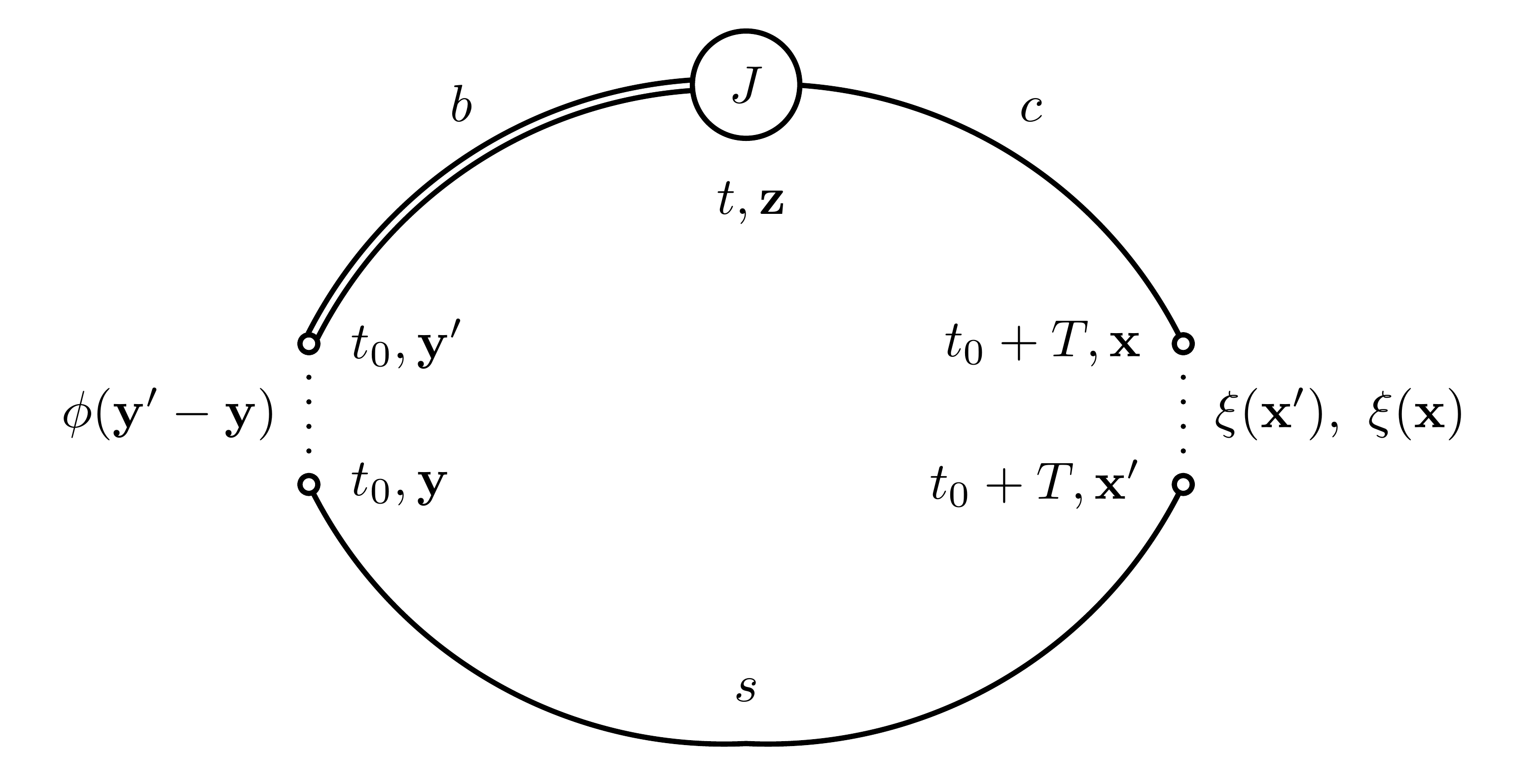
We calculate $B_{s}$ and $D_{s}$ meson two-point correlators and three-point correlators of the bottom-charm currents, $J_{\mu}$. We use smeared heavy-strange bilinears to represent the $B_{s}$ meson and incorporate both delta-function and Gaussian smearing, with a smearing radius of $r_{0}/a=5$ and $r_{0}/a=7$ on the coarse and fine ensembles, respectively. Three-point correlators are computed with the setup illustrated in Figure 1. The $B_{s}$ meson is created at time $t_{0}$ and a current $J_{\mu}$ inserted at timeslice $t$, between $t_{0}$ and $t_{0}+T$. The daughter $D_{s}$ meson is then annihilated at timeslice $t_{0}+T$. We use four values of $T$: 12, 13, 14, and 15 on the coarse lattices; and 21, 22, 23, and 24 on the fine lattices. We implement spatial sums at the source through the $U(1)$ random wall sources $\xi(x)$ and $\xi(x^{\prime})$ Na et al. (2010). We generate data for four different values of the $D_{s}$ meson momenta, $\vec{p}=2\pi/(aL)(0,0,0)$, $\vec{p}=2\pi/(aL)(1,0,0)$, $\vec{p}=2\pi/(aL)(1,1,0)$, and $\vec{p}=2\pi/(aL)(1,1,1)$, where $L$ is the spatial lattice extent.

Figure 1: Lattice setup for the three-point correlators. See accompanying text for details.

We fit $B_{s}$ meson two-point functions to a sum of decaying exponentials in Euclidean time, $t$,

$$C_{B_{s}}^{\beta,\alpha}(t)={} \sum_{i=0}^{N_{B_{s}}-1}b_{i}^{\beta}b_{i}^{\alpha\ast}e^{-E_{i}^{B_{s},\mathrm{sim}}t}$$

$$+\sum_{i=0}^{N_{B_{s}}^{\prime}-1}b_{i}^{\prime\,\beta}b_{i}^{\prime\,\alpha\ast}(-1)^{t}e^{-E_{i}^{\prime\,B_{s},\mathrm{sim}}t}.$$ (9)

Here the superscripts $\alpha$ and $\beta$ indicate the smearing associated with the $B_{s}$ meson source (delta function or Gaussian); the $b_{i}$ and $b_{i}^{\prime}$ are amplitudes associated with the ordinary non-oscillatory states and the oscillatory states that arise in the staggered quark formalism; the meson energies are $E_{i}^{B_{s},\mathrm{sim}}$ and $E_{i}^{\prime\,B_{s},\mathrm{sim}}$ for the non-oscillatory and oscillatory states, respectively; and $N_{B_{s}}^{(\prime)}$ is the number of exponentials included in the fit.

The ground state $B_{s}$ energy in NRQCD, $E_{0}^{B_{s},\mathrm{sim}}$, is related to the true energy in full QCD, $E_{0}^{B_{s}}$, by

$$E_{0}^{B_{s}}\equiv M_{B_{s}}=\frac{1}{2}\left[\overline{M}_{b\overline{b}}^{\mathrm{exp}}-E_{b\overline{b}}^{\mathrm{sim}}\right]+E_{0}^{B_{s},\mathrm{sim}},$$ (10)

because the $b$-quark rest mass has been integrated out in NRQCD. Here $\overline{M}_{b\overline{b}}^{\mathrm{exp}}$ is the spin-averaged $\Upsilon$ mass used to tune the $b$-quark mass and $aE_{b\overline{b}}^{\mathrm{sim}}$ was determined in Na et al. (2012). We tabulate the values for $aE_{b\overline{b}}^{\mathrm{sim}}$ in Table 3.

We fit the $D_{s}$ meson two-point functions to the form

$$C_{D_{s}}(t;\vec{p})={} \sum_{i=0}^{N_{D_{s}}-1}|d_{i}|^{2}\left[e^{-E_{i}^{D_{s}}t}+e^{-E_{i}^{D_{s}}(N_{t}-t)}\right]$$

$$+\sum_{i=0}^{N_{D_{s}}^{\prime}-1}{} |d_{i}^{\prime}|^{2}(-1)^{t}\left[e^{-E_{i}^{\prime\,D_{s}}t}+e^{-E_{i}^{\prime\,D_{s}}(N_{t}-t)}\right].$$ (11)

For the three-point correlator we use the fit ansatz

$$C_{J}^{\alpha}{} (t,T;\vec{p})=\sum_{i=0}^{N_{D_{s}}-1}\sum_{j=0}^{N_{B_{s}}-1}A_{ij}^{\alpha}e^{-E_{i}^{D_{s}}t}e^{-E_{j}^{B_{s},\mathrm{sim}}(T-t)}$$

$$+\sum_{i=0}^{N_{D_{s}}^{\prime}-1}\sum_{j=0}^{N_{B_{s}}-1}B_{ij}^{\alpha}(-1)^{t}e^{-E_{i}^{\prime\,D_{s}}t}e^{-E_{j}^{B_{s},\mathrm{sim}}(T-t)}$$

$$+\sum_{i=0}^{N_{D_{s}}-1}\sum_{j=0}^{N_{B_{s}}^{\prime}-1}C_{ij}^{\alpha}(-1)^{t}e^{-E_{i}^{D_{s}}t}e^{-E_{j}^{\prime\,B_{s},\mathrm{sim}}(T-t)}$$

$$+\sum_{i=0}^{N_{D_{s}}^{\prime}-1}\sum_{j=0}^{N_{B_{s}}^{\prime}-1}D_{ij}^{\alpha}(-1)^{T}e^{-E_{i}^{\prime\,D_{s}}t}e^{-E_{i}^{\prime\,B_{s},\mathrm{sim}}(T-t)}.$$ (12)

The amplitudes $A_{ij}^{\alpha}$ for energy levels $(i,j)$ depend on the current $J_{\mu}$, the daughter $D_{s}$ meson momentum $\vec{p}$, and the smearing of the $B_{s}$ meson source, $\alpha$.

The hadronic matrix element between $B_{s}$ and $D_{s}$ meson states is then given in terms of the ground state energies and amplitudes extracted from two- and three-point correlator fits by the relation

$$\langle D_{s}(\vec{p})|V^{\mu}|B_{s}\rangle=\frac{A_{00}^{\alpha}}{d_{0}b_{0}^{\alpha\ast}}\sqrt{2a^{3}E_{0}^{D_{s}}}\sqrt{2a^{3}M_{B_{s}}}.$$ (13)

For more details on this relation, see Section III of Na et al. (2015).

III Correlator fit and form factor results

We employ a Bayesian multi-exponential fitting procedure, based on the python packages lsqfit Lepage, G.P. (a) and corrfitter Lepage, G.P. (b), that has been used by the HPQCD collaboration for a wide range of lattice calculations. Statistical correlations between data points, and correlations between data and priors, are automatically captured with the gvar class Lepage, G.P. (c), which facilitates the straightforward manipulation of Gaussian-distributed random variables.

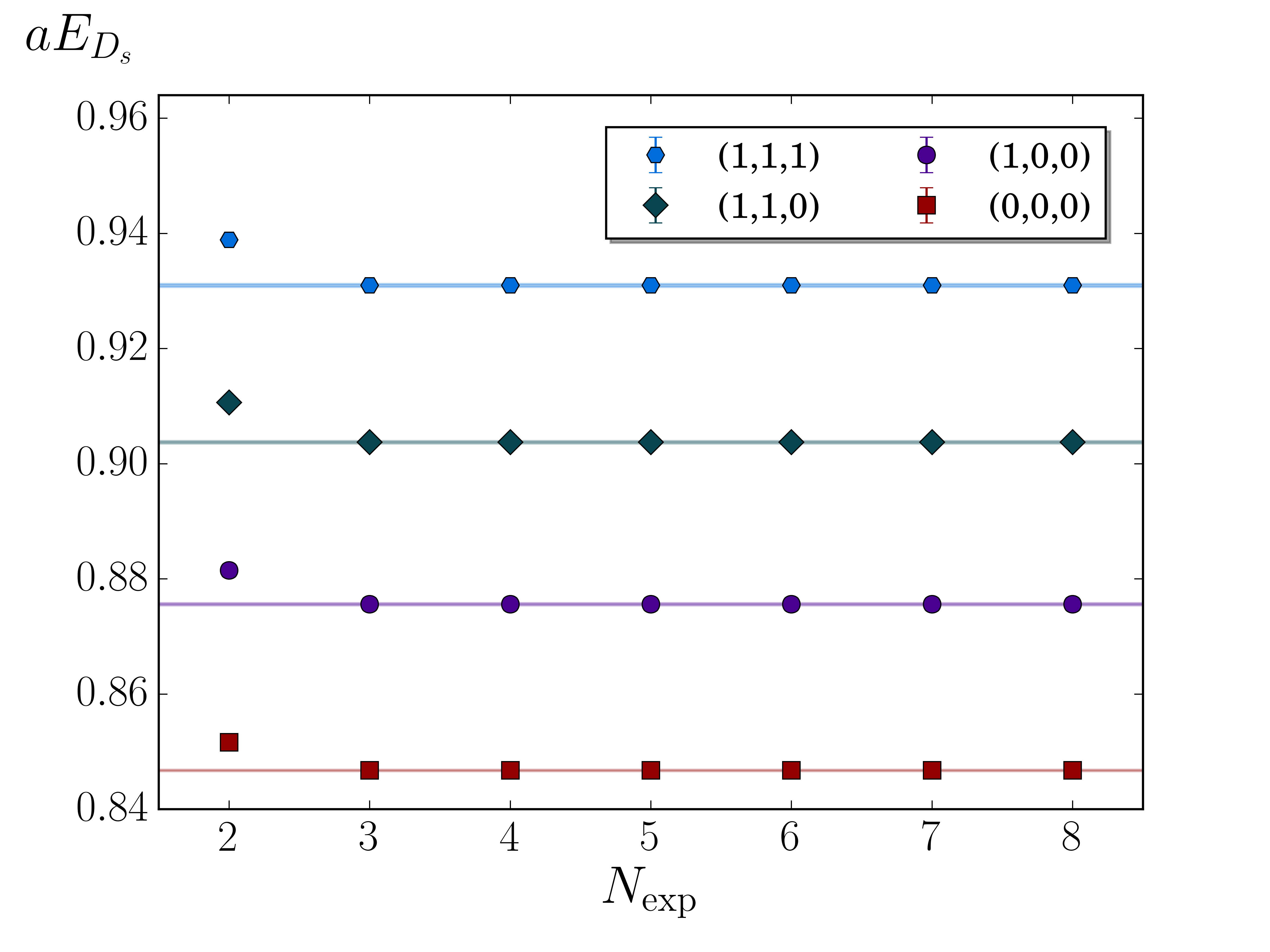
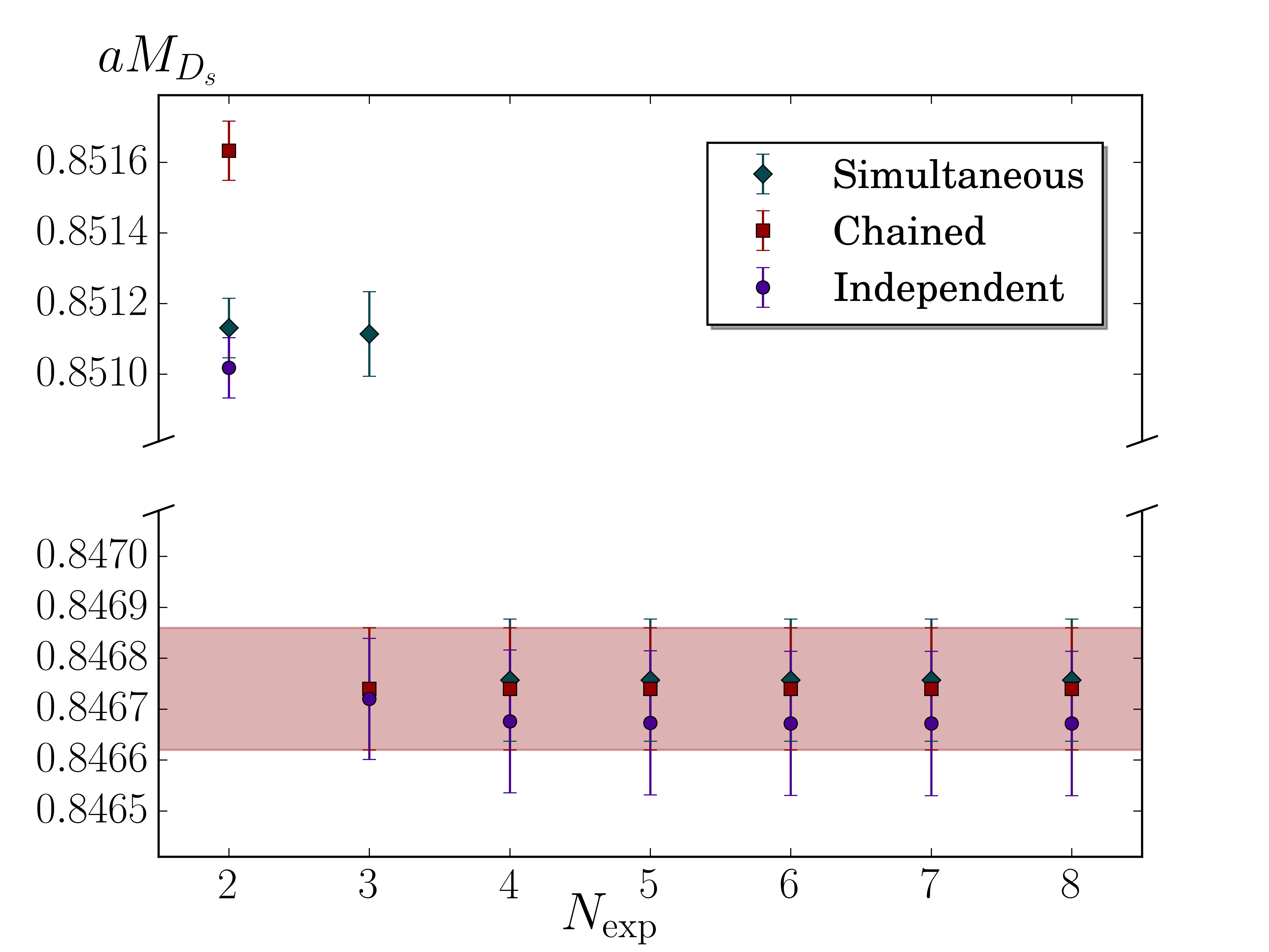
In this Bayesian multi-exponential approach, one uses a number of indicators of fit stability, consistency, and goodness-of-fit to check the fit results. For example, we check that, beyond a minimum number of exponentials, the fit results are independent of the number of exponentials included in the fit. Figure 2 illustrates the results of this test for the $D_{s}$ meson two-point fits on ensemble set F1. The upper panel presents our results for four values of the spatial momentum, plotted as a function of the number of exponentials included in the plot. The lower panel shows the results obtained from three types of fits: a simultaneous fit to correlator data for all four spatial momenta, plotted with blue diamonds; a chained fit (discussed in detail in Appendix A of Bouchard et al. (2014)) to correlator data for all four spatial momenta simultaneously, shown with red squares; and an “individual” fit, plotted with purple circles. These individual fits include the correlator data for just a single daughter meson momentum in each fit.

We take the result for $N_{\mathrm{exp}}=5$ from the chained fit as our final result for each momentum. These results are tabulated in Table 4 and shown in Figure 2 as shaded bands in each plot. All three fit approaches give consistent results, as seen in the lower panel of Figure 2, but the simultaneous fits, with or without chaining, have the advantage that they capture the correlations between momenta, which is then reflected in the uncertainty quoted in the fit results. The chained fits give slightly better values of reduced $\chi^{2}$. For example, for the ground state results plotted in the lower panel, the chained fits give $\chi^{2}/\mathrm{dof}=0.88$ for $N_{\mathrm{nexp}}=5$, while the simultaneous fits give $\chi^{2}/\mathrm{dof}=1.1$. Both fits include 164 degrees of freedom. In addition, the chained fits are about ten percent faster than the simultaneous fits—14.6s to generate all the data in the lower plot for the chained fit compared to 16.4s for the simultaneous fit. This is not an important consideration for the two-point fits, but becomes relevant for the larger three-point fits, which can take many hours. Choosing to use chained fits for both two- and three-point fits ensures a consistent approach throughout the fitting procedure.

Figure 2: Fit results for the $D_{s}$ meson two-point correlator as a function of the number of exponentials included in the fit on ensemble F1. The upper plot includes data for all four values of the spatial momentum of the $D_{s}$ meson. The lower plot compares the values for the ground state energy from the simultaneous fit with two alternative fitting strategies, which are described in the text, at zero spatial momentum. Note the magnified scale on the vertical axis in the lower panel.

Table 4: Fit results for the ground state energies of the $D_{s}$ meson at each spatial momentum $\vec{p}$. We take $N_{\mathrm{exp}}=5$ and fit all two-point correlator data simultaneously.

Set	$aM_{D_{s}}$	$aE_{D_{s}}(1,0,0)$	$aE_{D_{s}}(1,1,0)$	$aE_{D_{s}}(1,1,1)$
C1	1.18755(22)	1.21517(34)	1.24284(33)	1.27013(39)
C2	1.20090(30)	1.24013(56)	1.27822(61)	1.31543(97)
C3	1.19010(33)	1.23026(53)	1.26948(54)	1.30755(79)
F1	0.84674(12)	0.87559(19)	0.90373(20)	0.93096(26)
F2	0.84415(14)	0.87348(25)	0.90145(25)	0.92869(33)

As a further test of the two-point fits for the $D_{s}$ meson we determine the ratio $(M_{D_{s}}^{2}+\vec{p}^{2})/E_{D_{s}}^{2}$ on each ensemble. We plot the results in Figure 3. The shaded region corresponds to $1\pm\alpha_{s}(ap/\pi)^{2}$, where we set $\alpha_{s}=0.25$. In general, the data lie systematically above the relativistic value of unity, indicating that the statistical uncertainties of the fit results are sufficiently small that we can resolve discretization effects at ${\cal O}(\alpha_{s}(ap/\pi)^{2})$. These discretization effects are less than $0.5\%$ in the dispersion relation.

Figure 3: Dispersion relation for each ensemble. The shaded region corresponds to $1\pm\alpha_{s}(ap/\pi)^{2}$ where we take $\alpha_{s}=0.25$.

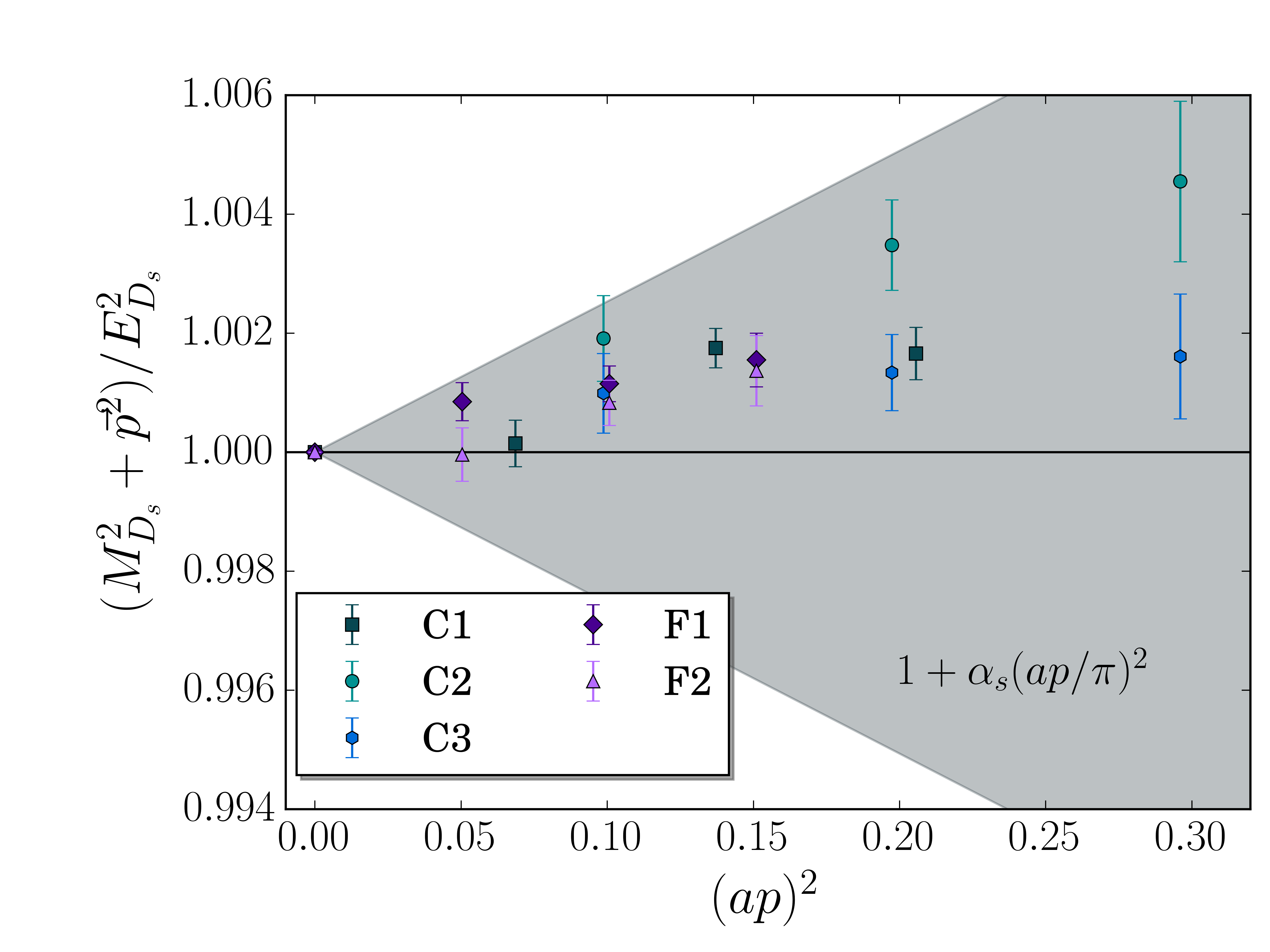
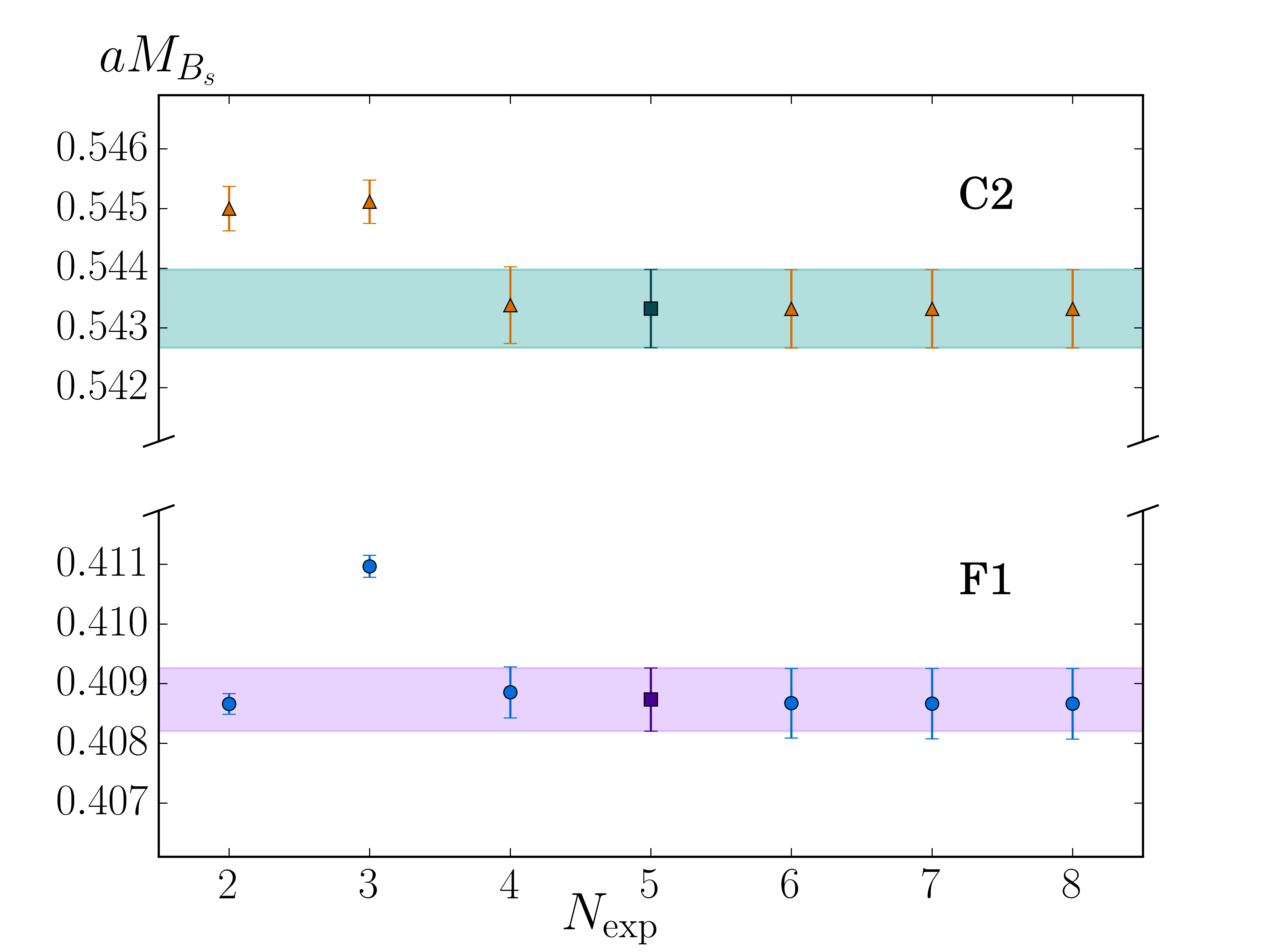
Figure 4 shows the corresponding two-point fit results for the ground state of the $B_{s}$ meson for ensemble sets C2 and F1. These ensemble sets have the same sea quark mass ratios, $m_{\ell}/m_{s}=1/5$ (see Table 1) and the difference between the results stems almost entirely from the lattice spacing. We take the values with $N_{\mathrm{exp}}=5$ as our final results, highlighted in the figure by the square data points and the shaded bands. We tabulate our final results in Table 5.

Figure 4: Fit results for the $B_{s}$ meson two-point correlator as a function of the number of exponentials included in the fit on two ensemble sets, C2 and F1. We plot our final results, for which $N_{\mathrm{exp}}=5$, as a green hexagon for C2 and a purple square for F1, with corresponding shaded bands.

Table 5: Fit results for the ground state $aE_{0}^{B_{s},\mathrm{sim}}$, on each ensemble set, with $N_{\mathrm{exp}}=5$.

C1	C2	C3	F1	F2
0.53714(60)	0.54332(65)	0.53657(86)	0.40873(53)	0.40819(44)

For the three-point correlator fits, we use a fitting procedure that diverges slightly from the approach taken in Na et al. (2015) and do not employ a “mixed” fitting strategy. Instead of combining “individual” and “master” fits (see Na et al. (2015) for full details), we use chained fits to correlators at all spatial momenta. This fitting approach ensures that we keep track of all statistical correlations between data at different momenta while maintaining fit stability, which was an issue for simultaneous fits attempted in Na et al. (2015).

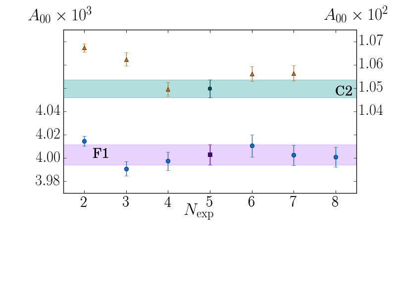
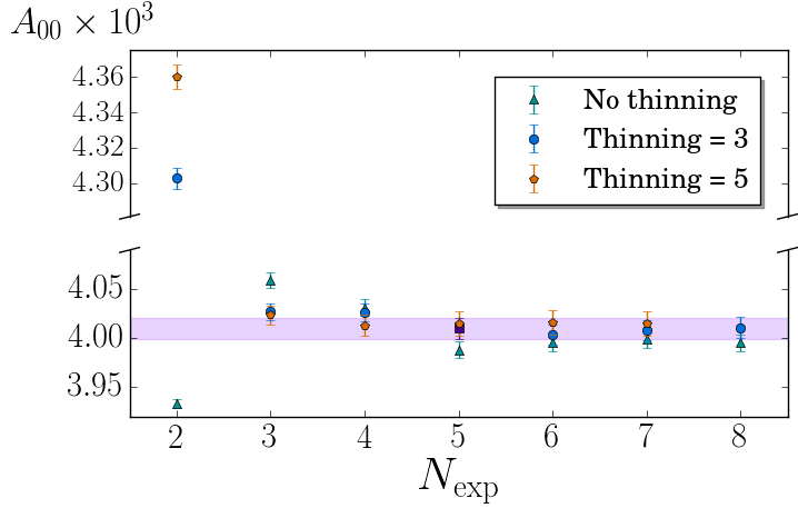
To improve stability and goodness-of-fit, we thin the three-point correlator data on the fine ensembles by keeping every third timeslice. We illustrate the stability of these fits with the number of exponentials in the fit in Figure 5.

Figure 5: Fit results for the three-point amplitudes as a function of the number of exponentials on two ensemble sets, C2 and F1. We fit to correlator data for all values of the spatial momentum simultaneously and thin by keeping every third timeslice. We plot our final results, for which $N_{\mathrm{exp}}=5$, as a green hexagon for C2 and a purple square for F1, with corresponding shaded bands. Note that the amplitudes on set C2 are approximately three times larger than the amplitudes on set F1, as indicated by the left (F1) and right (C2) vertical axes.

We test our choice by comparing fit results for the three-point amplitudes with thinning (keeping both every third and every fifth timeslice) and without thinning and plot the results in Figure 6. We do not consider thinning by an even integer, which removes information about the oscillatory states generated by the staggered quark action.

Figure 6: Fit results for the three-point amplitudes as a function of the number of exponentials for different choices of data thinning: no thinning, represented by turquoise triangles; keeping every third timeslice, represented by blue circles and the label “Thinning = 3”; and every fifth timeslice, shown by yellow pentagons and the label “Thinning = 5”. Our final result, for which we use thinning by every third timeslice and $N_{\mathrm{exp}}=5$, is shown as a purple square and the corresponding purple shaded band.

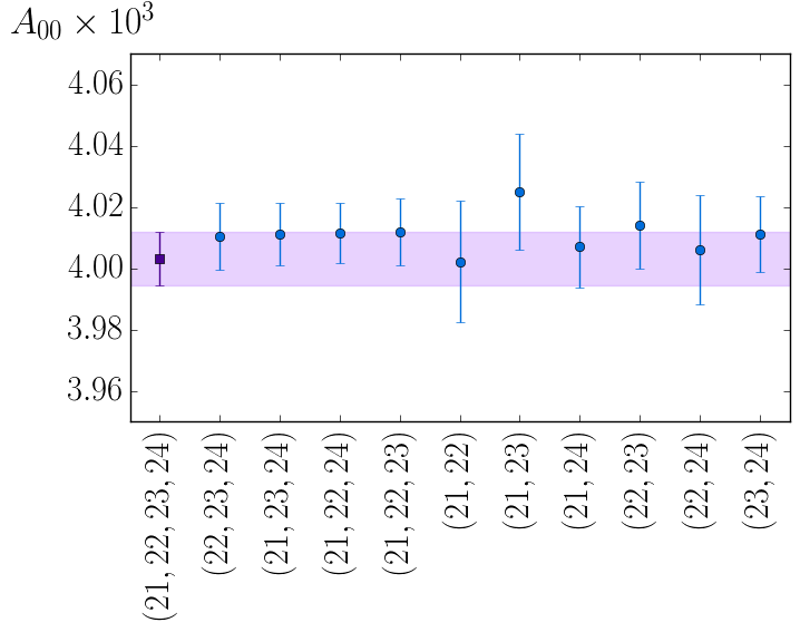
In Figure 7 we present results for the three-point fits when different combinations of source-sink separations, $T$, are used. For our final results we take the full set, $T=(12,13,14,15)$ on the coarse ensembles and $T=(21,22,23,24)$ on the fine ensembles.

Figure 7: Fit results for the three-point amplitude $A_{00}$ as a function of the number of source-sink separations, $T$, incorporated in the fit on ensemble set F1. We fit to correlator data for all values of the spatial momentum simultaneously and thin by keeping every third timeslice. For our final results we take the full set, $T=(12,13,14,15)$ on the coarse ensembles and $T=(21,22,23,24)$ on the fine ensembles, indicated by the first point, the purple square, and the purple shaded band. Fit results from other combinations of source-sink separations are plotted as blue circles.

We fit the three-point correlator data after matching the bottom-charm currents to full QCD, as described briefly in Section II and in more detail in Na et al. (2015). In Na et al. (2015) this approach was compared with fitting the data first and then matching to full QCD and, as expected, the results are in good agreement within errors.

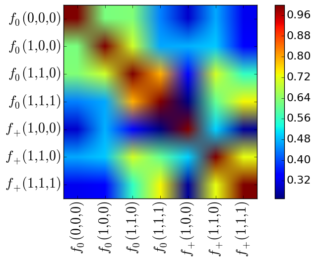
We summarize our final results for the form factors, $f_{0}(\vec{p})$ and $f_{+}(\vec{p})$, for each ensemble and $D_{s}$ momentum in Tables 7 and 7. We represent the correlations between form factors at different momenta as a heat map in Figure 8 for ensemble set F2.

Figure 8: Correlations between form factors at different momenta for the ensemble set F2.

Table 6: Final results for the form factor $f_{0}(\vec{p})$.

Set	$f_{0}(0,0,0)$	$f_{0}(1,0,0)$	$f_{0}(1,1,0)$	$f_{0}(1,1,1)$
C1	0.8885(11)	0.8754(14)	0.8645(13)	0.8568(13)
C2	0.8822(13)	0.8663(15)	0.8524(16)	0.8418(18)
C3	0.8883(13)	0.8723(16)	0.8603(16)	0.8484(21)
F1	0.90632(98)	0.8848(13)	0.8674(13)	0.8506(17)
F2	0.9047(12)	0.8855(16)	0.8667(15)	0.8487(19)

Table 7: Final results for the form factor $f_{+}(\vec{p})$.

Set	$f_{+}(1,0,0)$	$f_{+}(1,1,0)$	$f_{+}(1,1,1)$
C1	1.1384(35)	1.1081(20)	1.0827(21)
C2	1.1137(29)	1.0795(22)	1.0470(21)
C3	1.1260(34)	1.0912(24)	1.0552(28)
F1	1.1453(29)	1.0955(24)	1.0549(24)
F2	1.1347(42)	1.0905(26)	1.0457(33)

IV Chiral, continuum and kinematic extrapolations

The form factor results presented in the previous section are determined at finite lattice spacing, with sea quark masses that are heavier than their physical values. These form factors are therefore functions of the momentum transfer, the lattice spacing, and the sea quark masses. The form factors determined from experimental data are functions of a single kinematic variable only. Typically this variable is the momentum transfer, $q^{2}$, or the daughter meson energy, $E_{D_{s}}$, but the form factors can also be expressed in terms of the $w$-variable, defined by

$$w(q^{2})=1+\frac{q_{\mathrm{max}}^{2}-q^{2}}{2M_{B_{s}}M_{D_{s}}},$$ (14)

where $q_{\mathrm{max}}^{2}=(M_{B_{s}}-M_{D_{s}})^{2}\simeq$11.54\text{\,}\mathrm{G}\mathrm{e}\mathrm{V}^{2}$$ or the $z$-variable,

$$z(q^{2})=\frac{\sqrt{t_{+}-q^{2}}-\sqrt{t_{+}-t_{0}}}{\sqrt{t_{+}-q^{2}}+\sqrt{t_{+}-t_{0}}}.$$ (15)

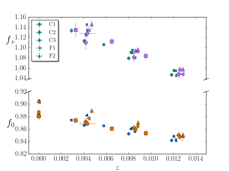
Here $t_{+}=(M_{B_{s}}+M_{D_{s}})^{2}$ and $t_{0}$ is a free parameter, which we take to be $t_{0}=q_{\mathrm{max}}^{2}$ to ensure consistency with the analysis of Na et al. (2015). In Figure 9 we compare our results for the form factors, $f_{0}(q^{2})$ and $f_{+}(q^{2})$, with the corresponding form factors for the $B\to D\ell\nu$ decay, taken from Na et al. (2015), as a function of the $z$-variable. From the plot, we see that there is little dependence on the light spectator quark species in the form factor results.

Figure 9: Form factor results for the $B_{s}\to D_{s}\ell\nu$ decay, compared to those for the $B\to D\ell\nu$ decay from Na et al. (2015), as function of $z$. We plot four sets of results, for $f_{0}(q^{2}(z))$ and $f_{+}(q^{2}(z))$ for both $B$ and $B_{s}$ meson decays. We distinguish the data in four ways. First, the shape of each data marker indicates the corresponding ensemble set, as shown in the legend in the upper left corner: squares represent set C1; diamonds set C2; circles C3; left-triangles F1; and triangles F2. Second, the upper set of points are those for $f_{+}(q^{2}(z))$ and the lower set of points show the data for $f_{0}(q^{2}(z))$, as indicated by the annotations. Third, the color of the points distinguishes the data as follows: the turquoise-green points represent $f_{+}^{B_{s}\to D_{s}}(q^{2}(z))$; the light purple points are $f_{+}^{B\to D}(q^{2}(z))$; the blue points are $f_{0}^{B_{s}\to D_{s}}(q^{2}(z))$; and the orange-yellow points are $f_{0}^{B\to D}(q^{2}(z))$. Finally, we distinguish the data by size: the larger markers represent the $B\to D\ell\nu$ decay, while the smaller points are from those for the $B_{s}\to D_{s}\ell\nu$ decay.

To relate the form factor results determined at finite lattice spacing and unphysical sea quark masses to experimental data, we must therefore perform continuum and chiral extrapolations, along with a kinematic extrapolation in terms of one of the choices of kinematic variable. We combine these extrapolations through the modified $z$-expansion, introduced in Na et al. (2010, 2011), and applied to $B_{(s)}$ heavy-light decays in Bouchard et al. (2013a, b); Bouchard et al. (2014). Our analysis of the chiral-continuum-kinematic extrapolation for $B_{s}\to D_{s}\ell\nu$ decay closely parallels that for the $B\to D\ell\nu$ decay in Na et al. (2015), so we only briefly outline the key components and refer the reader to Na et al. (2015) for details.

We express the dependence of the form factors on the $z$-variable through a modification of the BCL parameterization Bourrely et al. (2009)

$$f_{0}(q^{2}(z))={} \frac{1}{P_{0}}\sum_{j=0}^{J-1}a_{j}^{(0)}(m_{l},m_{l}^{\mathrm{sea}},a)z^{j},$$ (16)

$$f_{+}(q^{2}(z))={} \frac{1}{P_{+}}\sum_{j=0}^{J-1}a_{j}^{(+)}(m_{l},m_{l}^{\mathrm{sea}},a)$$

$$\qquad\times\left[z^{j}-(-1)^{j-J}\frac{j}{J}z^{J}\right].$$ (17)

Here the $P_{0,+}$ are Blaschke factors that take into account the effects of expected poles above the physical region,

$$P_{0,+}(q^{2})=\left(1-\frac{q^{2}}{M_{0,+}^{2}}\right),$$ (18)

where we take $M_{+}=M_{B_{c}^{\ast}}=$6.330(9)\text{\,}\mathrm{G}\mathrm{e}\mathrm{V}$$ Gregory et al. (2010), and $M_{0}=$6.42(10)\text{\,}\mathrm{G}\mathrm{e}\mathrm{V}$$. We find little dependence on the value of $M_{0}$, in line with the results of Na et al. (2015). The expansion coefficients $a_{j}^{(0,+)}$ include lattice spacing and light quark mass dependence and can be written as

$$a_{j}^{(0,+)}(m_{l},m_{l}^{\mathrm{sea}},a)=\widetilde{a}_{j}^{(0,+)}\widetilde{D}_{j}^{(0,+)}(m_{l},m_{l}^{\mathrm{sea}},a),$$ (19)

where the $\widetilde{D}_{j}^{(0,+)}$ include all lattice artifacts and chiral logarithms. These coefficients are given by

$$\widetilde{D}_{j}={} 1+c_{j}^{(1)}x_{\pi}+c_{j}^{(2)}x_{\pi}\log(x_{\pi})$$

$$\qquad+d_{j}^{(1)}\left(\frac{\delta x_{\pi}}{2}+\delta x_{K}\right)+d_{j}^{(2)}\delta x_{\eta_{s}}$$

$$\qquad+e_{j}^{(1)}\left(\frac{aE_{D_{s}}}{\pi}\right)^{2}+e_{j}^{(2)}\left(\frac{aE_{D_{s}}}{\pi}\right)^{4}$$

$$\qquad+m_{j}^{(1)}(am_{c})^{2}+m_{j}^{(2)}(am_{c})^{4},$$ (20)

where

$$x_{\pi,K,\eta_{s}}={} \frac{M_{\pi,K,\eta_{s}}^{2}}{(4\pi f_{\pi})^{2}},$$ (21)

$$\delta x_{\pi,K}={} \frac{(M_{\pi,K}^{\mathrm{AsqTad}})^{2}-(M_{\pi,K}^{\mathrm{HISQ}})^{2}}{(4\pi f_{\pi})^{2}},$$ (22)

$$\delta x_{\eta_{s}}={} \frac{(M_{\eta_{s}}^{\mathrm{HISQ}})^{2}-(M_{\eta_{s}}^{\mathrm{phys.}})^{2}}{(4\pi f_{\pi})^{2}},$$ (23)

and the $c_{j}^{(i)}$, $d_{j}^{(i)}$, $e_{j}^{(i)}$, and $m_{j}^{(i)}$ are fit parameters, along with the $\widetilde{a}_{j}^{(0,+)}$. We use the fit function form of Na et al. (2015), with a new fit parameter, $d_{j}^{(2)}$, to account for the tuning of the valence strange quark mass on each ensemble. We tabulate the meson masses required to calculate $\delta x_{\pi,K,\eta_{s}}$ in Table 2.

We further modify the $z$-expansion parameterization of the form factors to accommodate the systematic uncertainty associated with the truncation of the matching procedure at ${\cal O}(\alpha_{s},\Lambda_{\mathrm{QCD}}/m_{b},\alpha_{s}/(am_{b}))$. We introduce fit parameters $m_{\parallel}$ and $m_{\perp}$, with central value zero and width $\delta m_{\parallel,\perp}$ and re-scale the form factors, $f_{\parallel}$ and $f_{\perp}$ according to

$$f_{\parallel,\perp}\rightarrow(1+m_{\parallel,\perp})f_{\parallel,\perp}.$$ (24)

We take the systematic uncertainties in these fit parameters as 3% and refer the reader to the detailed discussion of this approach in Na et al. (2015).

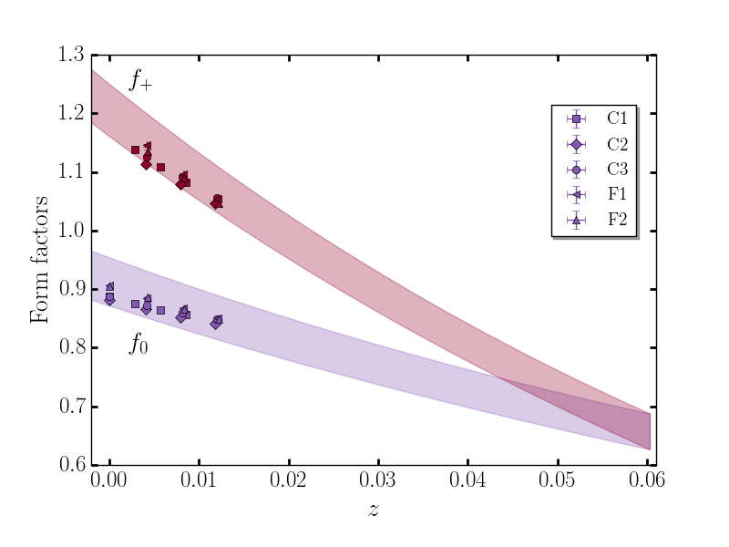
In Figure 10 we plot our fit results for $f_{0}(z)$, $f_{+}(z)$ as a function of the $z$-variable. We obtain a reduced $\chi^{2}$ of $\chi^{2}/\mathrm{dof}=1.2$ with 36 degrees of freedom (dof), with a quality factor of $Q=0.24$. The $Q$-value (or $p$-value) corresponds to the probability that the $\chi^{2}/\mathrm{dof}$ from the fit could have been larger, by chance, assuming the data are all Gaussian and consistent with each other. We plot the lattice data and the results of the chiral-continuum-kinematic extrapolation for $f_{+}(z)$ as the upper, red shaded band and for $f_{0}(z)$ as the lower, purple shaded band. We use the fit ansatz outlined above, including terms up to $z^{3}$ in the modified $z$-expansion, and refer to these results as the “standard extrapolation”. We tabulate our choice of priors and the fit results in Appendix A, and provide the corresponding $z$-expansion coefficients and their correlations in Table 11. Following Na et al. (2015) and the earlier work of Na et al. (2010, 2011), we group the priors into Group I and Group II variables, and add a third group. Broadly speaking, Group I priors are the typical fit parameters, Group II includes the input lattice scales and masses, and Group III priors are physical input masses. See the appendix of Na et al. (2015) for more details.

Figure 10: Fit results from the “standard extrapolation” fit ansatz detailed in the text. The purple data points show the fit results at finite lattice spacing and the red and purple shaded bands are the physical extrapolations.

To test the convergence of our fit ansatz, we follow a procedure similar to that outlined in Na et al. (2015). This can be summarized as modifying the fit ansatz in the following ways:

1. include terms up to $z^{2}$ in the $z$-expansion;

2. include terms up to $z^{4}$ in the $z$-expansion;

3. add light-quark mass dependence to the fit parameters $m_{j}^{(i)}$;

4. add strange-quark mass dependence to the fit parameters $m_{j}^{(i)}$;

5. add bottom-quark mass dependence to the fit parameters $m_{j}^{(i)}$;

6. include discretization terms up to $(am_{c})^{2}$;

7. include discretization terms up to $(am_{c})^{6}$;

8. include discretization terms up to $(aE_{D_{s}}/\pi)^{2}$;

9. include discretization terms up to $(aE_{D_{s}}/\pi)^{6}$;

10. omit the $x_{\pi}\log(x_{\pi})$ term;

11. incorporate a 2% uncertainty for higher-order matching contributions;

12. incorporate a 4% uncertainty for higher-order matching contributions;

13. incorporate 4% and 2% uncertainties on coarse and fine ensembles, respectively, for higher-order matching contributions.

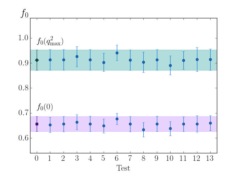
We show the results of these modifications in Figure 11. This plot demonstrates that the fit has converged with respect to a variety of modifications of the chiral-continuum-kinematic extrapolation ansatz. As part of this process, we also tested the significance of the Blaschke factor in the fit results. In line with the results of Na et al. (2015), we found that, while the results agreed within uncertainties, removing the Blaschke lowered the central value and increased the uncertainty of the result. This test is not strictly a test of convergence and is therefore not included in Figure 11.

Figure 11: Fit results from modifications to the “standard extrapolation” fit ansatz, plotted as blue circles representing the form factor $f_{0}$ at $q^{2}=0$ (the lower set of data points) and at $q^{2}=q^{2}_{\mathrm{max}}$ (the upper set of points). The test numbers labeling the horizontal axis correspond to the modifications listed in the text. The first data point, the purple square for $f_{0}(q^{2}=0)$ and turquoise diamond for $f_{0}(q^{2}_{\mathrm{max}})$, are the “standard extrapolation” fit results, which are also represented by the purple and turquoise shaded bands, respectively.

To determine the ratio of form factors, we simultaneously fit the lattice form factor data for the $B_{s}\to D_{s}\ell\nu$ and $B\to D\ell\nu$ decays in a single script. We take the form factor results from Table III of Na et al. (2015) for the $B\to D\ell\nu$ decay. Fitting the results simultaneously ensures that statistical correlations between the two data sets, such as those stemming from the lattice spacing determination on each ensemble set, are included in the final result for the ratio at zero momentum transfer. We do not re-analyze the $B\to D\ell\nu$ to account for statistical correlations between the correlators themselves, which have negligible effect on the final result, given the current precision. This analysis would require fitting both $B\to D\ell\nu$ and $B_{s}\to D_{s}\ell\nu$ two- and three-point correlators simultaneously. To ensure that these statistical correlations are not important, we tested the correlations between the three-point correlators on different ensemble sets. We show an example of the corresponding correlations as a heat map in Figure 12, from which one can see that statistical correlations are less than $\sim 0.6$. We have found that correlations of this size have negligible impact at our current level of precision.

Figure 12: Correlations between $B\to D\ell\nu$ and $B_{s}\to D_{s}\ell\nu$ ensemble-averaged, three-point correlators for ensemble set C1. The data correspond to a single $B_{(s)}$ meson source with Gaussian smearing $r_{0}/a=5$, a source-sink separation of $T=13$ and with $a\vec{p}_{D_{(s)}}=(0,0,0)$.

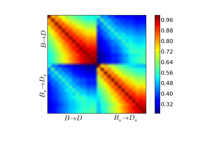
We fit the form factor data using the standard extrapolation ansätze for both the $B\to D\ell\nu$ and $B_{s}\to D_{s}\ell\nu$ data. For the $B_{s}\to D_{s}\ell\nu$ decay, we choose the priors for the coefficients in the modified $z$-expansion to be equal to those for the corresponding expression for the $B\to D\ell\nu$ $z$-expansion. These priors reflect the close agreement between the values for the $B\to D\ell\nu$ and $B_{s}\to D_{s}\ell\nu$ decays, illustrated in Figure 9. We list our choice of priors and the fit results for the ratio of form factors in Appendix A, and provide the corresponding $z$-expansion coefficients and their correlations in Table 12.

V Results

V.1 Form factors

We plot our final results for the form factors, $f_{0}(q^{2})$ and $f_{+}(q^{2})$, as a function of the momentum transfer, $q^{2}$, in Figure 13.

Figure 13: Chiral and continuum extrapolated form factors, $f_{0}(q^{2})$ (lower band) and $f_{+}(q^{2})$ (upper band), as a function of the momentum transfer.

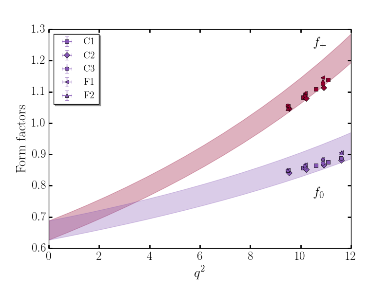
Our final result for the form factor at zero momentum transfer is

$$f_{0}^{B_{s}\to D_{s}}(0)=f_{+}^{B_{s}\to D_{s}}(0)=0.656(31).$$ (25)

We provide an estimate of the error budget for this result in Table 8. For the ratio of form factors, we find

$$\frac{f_{0}^{B_{s}\to D_{s}}(M_{\pi}^{2})}{f_{0}^{B\to D}(M_{K}^{2})}=1.000(62),$$ (26)

and

$$\frac{f_{0}^{B_{s}\to D_{s}}(M_{\pi}^{2})}{f_{0}^{B\to D}(M_{\pi}^{2})}=1.006(62),$$ (27)

with corresponding error budgets in Table 9. We show the extrapolation bands as a function of momentum transfer for both $B_{s}\to D_{s}$ (purple hatched band) and $B\to D$ (plain turquoise band) semileptonic decays in Figure 14.

Figure 14: Chiral and continuum extrapolated form factors, $f_{0}(q^{2})$ (lower band) and $f_{+}(q^{2})$ (upper band), as a function of the momentum transfer, for both $B_{s}\to D_{s}$ (purple hatched band) and $B\to D$ (plain turquoise band) semileptonic decays. The lattice data for each decay cannot be distinguished on this plot and are therefore not included. See Figure 10 for a detailed plot of the results for the form factors at finite lattice spacing for both decays.

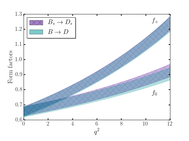
We find agreement, within errors, with the results of Bailey et al. (2012), which are

$$\frac{f_{0}^{B_{s}\to D_{s}}(M_{\pi}^{2})}{f_{0}^{B\to D}(M_{K}^{2})}[\mathrm{FNAL/MILC}]={} 1.046(46)$$ (28)

$$\frac{f_{0}^{B_{s}\to D_{s}}(M_{\pi}^{2})}{f_{0}^{B\to D}(M_{\pi}^{2})}[\mathrm{FNAL/MILC}]={} 1.054(50).$$ (29)

Here we have combined the uncertainties quoted in Bailey et al. (2012), which are statistical and systematic, in quadrature.

For the form factor at zero recoil, $f_{+}(q^{2}_{\mathrm{max}})$, which is often quoted as

$${\cal G}(1)=\frac{2\sqrt{\kappa}}{1+\kappa}f_{+}(q_{\mathrm{max}}^{2}),$$ (30)

where $\kappa=M_{D_{s}}/M_{B_{s}}$, we find

$${\cal G}(1)=1.068(40).$$ (31)

This result is in good agreement with the value of ${\cal G}(1)=1.052(46)$ determined in Atoui et al. (2014), with a slightly smaller uncertainty. The corresponding values for the $B\to D\ell\nu$ form factors are ${\cal G}^{B\to D}(1)=1.035(40)$ Na et al. (2015) and ${\cal G}^{B\to D}(1)=1.058(9)$ Bailey et al. (2012) (where the quoted uncertainty includes only statistical uncertainties).

The slope of the form factor, $f_{+}(q^{2})$, is given by

$$\rho^{2}(w)=-\frac{{\cal G}^{\prime}(w)}{{\cal G}(w)},$$ (32)

where the derivative is with respect to the $w$-variable of Equation (14). In the CLN parameterization, Caprini et al. (1998), the form factor is then parameterized by

$${\cal G}(w)={\cal G}(1)\Big{[}1-8\rho^{2}z+(51\rho^{2}-10)z^{2}-(252\rho^{2}-84)z^{3}\Big{]},$$ (33)

with $z=z(w)$ the $z$-variable of the previous section:

$$z(w)=\frac{\sqrt{w+1}-\sqrt{2}}{\sqrt{w+1}+\sqrt{2}}.$$ (34)

We obtain

$$\rho^{2}(1)=1.244(76)$$ (35)

for the slope of the form factor.

Experimental data for the $B\to D\ell\nu$ decay is typically presented in the form $|V_{cb}|{\cal G}(1)$, since the differential decay rate for the $B_{(s)}\to D_{(s)}\ell\nu$ decay can be written as

$$\frac{d\Gamma(B_{(s)}\to D_{(s)}\ell\nu)}{dw}={} \frac{G_{F}^{2}}{48\pi^{3}}M_{D_{(s)}}^{3}(M_{B_{(s)}}+M_{D_{(s)}})^{2}$$

$$\times(w^{2}-1)^{3/2}|V_{cb}|^{2}|{\cal G}(w)|^{2},$$ (36)

where $G_{F}$ is the Fermi constant. In this form, lattice results for the form factor ${\cal G}(1)$ provide the normalization required to extract $|V_{cb}|$ from experimental data. Incorporating the slope of the form factor, $\rho^{2}(w)$, helps further tighten experimental determinations of $|V_{cb}|$. An even more powerful approach incorporates the full kinematic dependence on the scalar and vector form factors, in combination with experimental data over a range of momentum transfer Na et al. (2015); Huschle et al. (2015). When combined with our form factor results, future experimental data for the $B_{s}\to D_{s}\ell\nu$ decay will provide a new method to extract $|V_{cb}|$ and may shed light on the long-standing tension between exclusive and inclusive determinations of $|V_{cb}|$.

V.2 Form factor error budget

We tabulate the errors in the form factors at zero momentum transfer, Equation (25), in Table 8.

Table 8: Error budget for the form factors at zero momentum transfer, $f_{0}(0)=f_{+}(0)$, for the $B_{s}\to D_{s}\ell\nu$ semileptonic decay. We describe each source of uncertainty in more detail in the accompanying text.

Type	Partial uncertainty (%)
Statistical	1.22
Chiral extrapolation	0.80
Quark mass tuning	0.66
Discretization	2.47
Kinematic	0.71
Matching	2.21
total	3.70

The sources of uncertainty listed in Table 8 are:

Statistical

The statistical uncertainties include the two- and three-point correlator fit errors and those associated with the lattice spacing determination, $r_{1}$ and $r_{1}/a$.

Chiral extrapolation

This uncertainty includes the valence and sea quark mass extrapolation errors and chiral logarithms in the chiral-continuum extrapolation. These effects correspond to the fit parameters $c_{j}^{i}$ in Equation (IV).

Quark mass tuning

Uncertainties arising from tuning errors in the light and strange quark masses at finite lattice spacing, including partial quenching effects between the HISQ valence and AsqTad sea quarks. These uncertainties are generally very small.

Discretization

Discretization effects incorporate the $(am_{c})^{n}$ and $(aE_{D_{s}}/\pi)^{n}$ terms in the modified $z$-expansion. These effects are the dominant source of uncertainty in our results.

Kinematic

These uncertainties stem from the $z$-expansion coefficients and the locations of the poles in the Blaschke factors.

Matching

Matching errors arise from the $m_{\perp,\parallel}$ fit parameters discussed in the previous section. Perturbative matching uncertainties are the second-largest source of uncertainty in our final results. We propagate these uncertainties from the large momentum-transfer region, for which we have lattice results, to zero momentum-transfer.

The uncertainties associated with physical meson mass input errors and finite volume effects, which are both less than $0.01\%$, are not included in these estimates, because they are negligible contributions to the final error budget. In our error budget, we also neglect uncertainties from electromagnetic effects, isospin breaking, and the effects of quenching in the charm quark in the gauge ensembles.

In Table 9 we list the uncertainties in the form factor ratios, Equations (26) and (27). These uncertainties are dominated by those coming from the $B\to D\ell\nu$ decay Na et al. (2015).

Table 9: Error budget for the ratio of the form factors, $f_{0}^{B_{s}\to D_{s}}(M_{\pi}^{2})/f_{0}^{B\to D}(M_{K}^{2})$ (second column) and $f_{0}^{B_{s}\to D_{s}}(M_{\pi}^{2})/f_{0}^{B\to D}(M_{\pi}^{2})$ (third column). We describe each source of uncertainty in more detail in the accompanying text.

Type	Partial uncertainty (%)
	$\frac{\vphantom{\big{[}}f_{0}^{B_{s}\to D_{s}}(M_{\pi}^{2})}{\vphantom{\big{[}}f_{0}^{B\to D}(M_{K}^{2})}$	$\frac{\vphantom{\big{[}}f_{0}^{B_{s}\to D_{s}}(M_{\pi}^{2})}{\vphantom{\big{[}}f_{0}^{B\to D}(M_{\pi}^{2})}$
Statistical	2.28	2.32
Chiral extrapolation	1.22	1.22
Quark mass tuning	0.81	0.81
Discretization	3.48	3.49
Kinematic	1.38	1.43
Matching	0.07	0.05
total	6.15	6.18

V.3 Semileptonic decay phenomenology

With our results for the ratio of the form factors, $f_{0}^{B_{s}\to D_{s}}/f_{0}^{B\to D}$, in Equations (26) and (27), we can now determine the ratio of fragmentation fractions. LHCb presents their measurement of the these ratios in the form Aaij et al. (2011)

$$\frac{f_{s}}{f_{d}}={} 0.310(30)_{\mathrm{stat.}}(21)_{\mathrm{syst.}}\frac{1}{{\cal N}_{a}{\cal N}_{F}},$$ (37)

$$\frac{f_{s}}{f_{d}}={} 0.307(17)_{\mathrm{stat.}}(23)_{\mathrm{syst.}}\frac{1}{{\cal N}_{a}{\cal N}_{e}{\cal N}^{\prime}_{F}},$$ (38)

where the ${\cal N}_{a}$ parameterize deviations from naive factorization and ${\cal N}_{e}$ is an electroweak correction factor to account for $W$-exchange. The dependence on the form factors is expressed in ${\cal N}_{F}$ and ${\cal N}^{\prime}_{F}$, which are given in Equation (2). For convenience, we repeat those expressions here:

$${\cal N}_{F}=\left[\frac{f_{0}^{(s)}(M_{\pi}^{2})}{f_{0}^{(d)}(M_{K}^{2})}\right]^{2}\quad\mathrm{and}\quad{\cal N}^{\prime}_{F}=\left[\frac{f_{0}^{(s)}(M_{\pi}^{2})}{f_{0}^{(d)}(M_{\pi}^{2})}\right]^{2}.$$ (39)

These ratios are relevant to the extraction of the fragmentation fraction ratios from the branching fraction ratios

$$\frac{{\cal B}(\overline{B}_{s}^{0}\to D_{s}^{+}\pi^{-})}{{\cal B}(\overline{B}^{0}\to D^{+}K^{-})}\quad\mathrm{and}\quad\frac{{\cal B}(\overline{B}_{s}^{0}\to D_{s}^{+}\pi^{-})}{{\cal B}(\overline{B}^{0}\to D^{+}\pi^{-})},$$ (40)

respectively.

Using our results in Equations (26) and (27), we obtain

$${\cal N}_{F}={} 1.00(12),$$ (41)

$${\cal N}^{\prime}_{F}={} 1.01(12).$$ (42)

These results are uncorrelated with the other factors in Equations (37) and (38), so that we can update the LHCb result for the fragmentation ratio directly. Using the values of ${\cal N}_{a}=1.00(2)$ and ${\cal N}_{e}=0.966(75)$ Fleischer et al. (2010, 2011), we find

$$\frac{f_{s}}{f_{d}}=0.310(30)_{\mathrm{stat.}}(21)_{\mathrm{syst.}}(6)_{theor.}(38)_{\mathrm{latt.}}$$ (43)

by using ${\cal N}_{F}$ for the ${\cal B}(\overline{B}_{s}^{0}\to D_{s}^{+}\pi^{-})/{\cal B}(\overline{B}^{0}\to D^{+}K^{-})$ channel. The uncertainties in this result are: the experimental statistical and systematic uncertainties; the uncertainty associated with ${\cal N}_{a}$; and the uncertainties in our lattice input, ${\cal N}_{F}$. We assume no correlations in these uncertainties. For the ${\cal B}(\overline{B}_{s}^{0}\to D_{s}^{+}\pi^{-})/{\cal B}(\overline{B}^{0}\to D^{+}\pi^{-})$ channel, we obtain

$$\frac{f_{s}}{f_{d}}=0.307(16)_{\mathrm{stat.}}(21)_{\mathrm{syst.}}(23)_{\mathrm{theor.}}(44)_{\mathrm{latt.}}$$ (44)

from ${\cal N}^{\prime}_{F}$.

These results are in agreement with the result determined in Bailey et al. (2012),

$$\frac{f_{s}}{f_{d}}=0.286(16)_{\mathrm{stat.}}(21)_{\mathrm{syst.}}(26)_{\mathrm{latt.}}(22)_{\mathrm{Ne}}.$$ (45)

Both of these lattice results are a little higher than that quoted in Khachatryan et al. (2015) of $f_{s}/f_{d}=0.259(15)$ or the average value of $f_{s}/f_{d}=0.267^{+22}_{-20}$ determined in Aaij et al. (2012), but all results agree within the quoted uncertainties.

The ratio

$$R(D)=\frac{{\cal B}(B\to D\tau\nu)}{{\cal B}(B\to D\ell\nu)}$$ (46)

measures the ratio of branching fraction of the semileptonic decay to the $\tau$ lepton to the branching fraction to an electron or muon (represented by $\ell$). The experimental measurements of this branching fraction ratio are currently in tension with the Standard Model result. The global experimental average is Lees et al. (2012, 2013); Huschle et al. (2015); Amhis et al. (2016b)

$$R(D)_{\mathrm{exp.}}=0.391(41)_{\mathrm{stat.}}(28)_{\mathrm{sys.}},$$ (47)

a value that is approximately 4$\sigma$ from the theoretical expectation

$$R(D)_{\mathrm{theor.}}=0.299(7),$$ (48)

where we have taken the mean of the results in Kamenik and Mescia (2008); Bailey et al. (2012); Na et al. (2015), and combined uncertainties in quadrature, neglecting any correlations for simplicity, because a full analysis of this result is beyond the scope of this work.

We present the first calculation from lattice QCD of the corresponding ratio for the semileptonic $B_{s}\to D_{s}\ell\nu$ decay,

$$R(D_{s})=\frac{{\cal B}(B_{s}\to D_{s}\tau\nu)}{{\cal B}(B_{s}\to D_{s}\ell\nu)}.$$ (49)

This ratio has not been experimentally measured and this provides an opportunity for lattice QCD to make a clear prediction of the value expected from the Standard Model. Using the form factor results of the previous section, we find

$$R(D_{s})=0.314(6).$$ (50)

We provide a complete error budget for this ratio in Table 10 and plot the differential branching fractions for $B_{s}\to D_{s}\mu\nu$ and $B_{s}\to D_{s}\tau\nu$ as functions of the momentum transfer in Figure 15.

Figure 15: Differential branching fractions for the $B_{s}\to D_{s}\mu\nu$ (hatched magenta band) and $B_{s}\to D_{s}\tau\nu$ (purple band) decays.

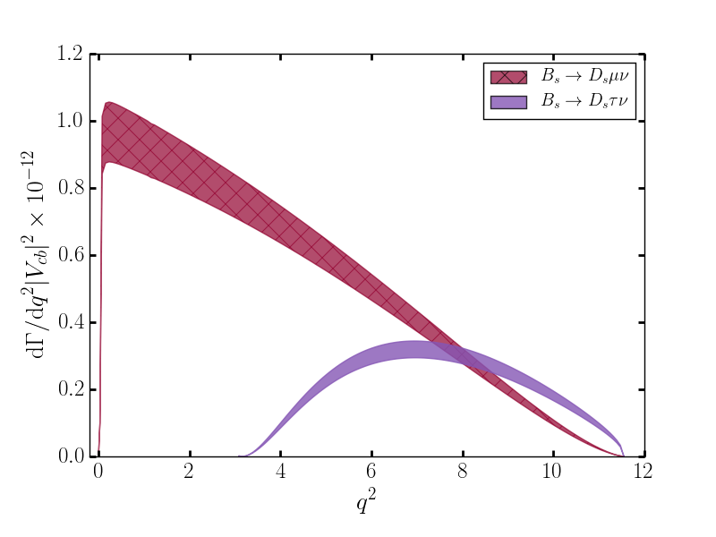
This result is larger, and about three time more precise, than the prediction of $R(D_{s})=0.274^{+20}_{-19}$ Bhol (2014), where the form factors were determined from a relativistic quark model.

Table 10: Error budget for the branching fraction ratio $R(D_{s})$. We describe each source of uncertainty in more detail in the accompanying text. The uncertainties associated with discretization effects is no longer the dominant source of uncertainty, because the discretization effects largely cancel in the ratio.

Type	Partial uncertainty (%)
Statistical	0.90
Chiral extrapolation	0.16
Quark mass tuning	0.19
Discretization	0.84
Kinematic	1.13
Matching	1.05
total	1.94

VI Summary

We have presented a lattice study of the $B_{s}\to D_{s}\ell\nu$ semileptonic decay over the full kinematic range of momentum transfer and determined the form factors, $f_{0}^{B_{s}\to D_{s}}(q^{2})$ and $f_{+}^{B_{s}\to D_{s}}(q^{2})$. Combining these results with a previous determination of the corresponding form factors for the $B\to D\ell\nu$ decay Na et al. (2015), we extracted the ratios $f_{0}^{B_{s}\to D_{s}}(M_{\pi}^{2})/f_{0}^{B\to D}(M_{K}^{2})$ and $f_{0}^{B_{s}\to D_{s}}(M_{\pi}^{2})/f_{0}^{B\to D}(M_{\pi}^{2})$. From these ratios we computed the fragmentation fraction ratio $f_{s}/f_{d}$, an important ingredient in experimental determinations of $B_{s}$ meson branching fractions at hadron colliders, particularly for the rare decay ${\cal B}(B_{s}\rightarrow\mu^{+}\mu^{-})$. In addition, we predict $R(D_{s})$, the ratio of the branching fractions of the semileptonic $B_{s}$ decay to tau and to electrons and muons.

There are a number of tensions between experimental measurements and theoretical expectations for semileptonic decays of the $B$ meson. These tensions include the branching fraction ratios, $R(D^{(\ast)})$, and determinations of $|V_{cb}|$ from exclusive and inclusive decays. Future experimental measurements of semileptonic decays of $B_{s}$ mesons, in conjunction with our results for the form factors and for $R(D_{s})$, may provide some insight into these tensions.

Our result for the form factor at zero recoil, ${\cal G}(1)$, presented in Equation (31), is consistent with an earlier determination by the ETM collaboration Atoui et al. (2014). Moreover, our results for the form factor ratios $f_{0}^{B_{s}\to D_{s}}(M_{\pi}^{2})/f_{0}^{B\to D}(M_{K}^{2})$ and $f_{0}^{B_{s}\to D_{s}}(M_{\pi}^{2})/f_{0}^{B\to D}(M_{\pi}^{2})$, given in Equations (26) and (27), are in agreement with the values obtained by the FNAL/MILC collaborations. Our determination of this ratio incorporates correlations between the form factors for both decay channels, but the quoted uncertainty does not include the statistical correlations between the raw correlator data, which are negligible at the current level of precision. We determine values for the fragmentation fraction ratio, $f_{s}/f_{d}$, Equations (43) and (44). These results have larger uncertainties associated with the form factor inputs than those determined in Bailey et al. (2012). Finally, we give the branching fraction ratio, $R(D_{s})$, in Equation (50).

The dominant uncertainty in the form factors for the $B_{s}\to D_{s}\ell\nu$ decay arises from the discretization effects, with a significant contribution from the matching to full QCD. Higher order calculations in lattice perturbation theory with the highly improved actions employed in this calculation are currently unfeasible, so we are exploring ways to reduce matching errors by combining results calculated using NRQCD with those determined with an entirely relativistic formulation for the $b$-quark. This approach is outlined in Bouchard et al. (2014); Na et al. (2015).

The LHC is scheduled to significantly improve the statistical uncertainties in experimental measurements of $B_{s}$ decays with more data over the next decade. Currently, the most precise determinations of the fragmentation fraction ratio, $f_{s}/f_{d}$, are those measured in situ at the LHC. To improve the theoretical calculations of this ratio requires several advances. At present the lattice form factor results are the largest source of uncertainty in the theoretical result for the ratio, but this could be improved with a suitable global averaging procedure, such as that undertaken in Aoki et al. (2016).

Further improvements in the uncertainty in the Standard Model expectation of the ratio of the fragmentation fractions will ultimately require concerted effort to reduce all sources of uncertainty, not just those from lattice QCD. Improved theoretical determinations of the fragmentation fraction ratio will be necessary to take full advantage of the better statistical precision of future experimental results and shed light on current tensions in the heavy quark flavor sector.

Appendix A Reconstructing form factors

In this appendix we provide our fit results for the coefficients of the $z$-expansion, for both the $B_{s}\to D_{s}\ell\nu$ decay and the ratio of the $B\to D\ell\nu$ and $B_{s}\to D_{s}\ell\nu$ decays. We also tabulate our choice of priors for the chiral-continuum extrapolation for the $B_{s}\to D_{s}\ell\nu$ decay.

Table 11: Coefficients of $z$-expansion and the corresponding Blaschke factors (first row), and their covariances, for the $B_{s}\to D_{s}\ell\nu$ decay. The rows correspond to the columns, moving from to bottom and left to right, respectively.

$a_{0}^{(0)}$	$a_{1}^{(0)}$	$a_{2}^{(0)}$	$P_{0}$	$a_{0}^{(+)}$	$a_{1}^{(+)}$	$a_{2}^{(+)}$	$P_{+}$
0.658(31)	-0.10(30)	1.3(2.8)	6.330(9)	0.858(32)	-3.38(41)	0.6(4.7)	6.43(10)
9.53401$\times 10^{-4}$	-3.03547$\times 10^{-3}$	-5.42391$\times 10^{-3}$	8.76501$\times 10^{-4}$	5.94503$\times 10^{-4}$	1.58251$\times 10^{-3}$	1.60091$\times 10^{-2}$	6.15598$\times 10^{-6}$
	9.03097$\times 10^{-2}$	-0.101760	-1.69040$\times 10^{-2}$	4.46248$\times 10^{-4}$	2.36283$\times 10^{-2}$	4.56659$\times 10^{-2}$	-1.29286$\times 10^{-4}$
		8.02283	3.96101$\times 10^{-3}$	8.48079$\times 10^{-3}$	0.104246	0.760797	-8.23960$\times 10^{-7}$
			1.06275$\times 10^{-2}$	-3.65165$\times 10^{-5}$	-1.30241$\times 10^{-3}$	-3.70251$\times 10^{-3}$	8.06159$\times 10^{-5}$
				1.00761$\times 10^{-3}$	-4.23358$\times 10^{-3}$	-2.64511$\times 10^{-2}$	9.42502$\times 10^{-6}$
					0.165251	-0.617234	-1.88031$\times 10^{-4}$
						22.49292	6.83236$\times 10^{-5}$
							8.09911$\times 10^{-5}$

Table 12: Coefficients and Blaschke factors for the $z$-expansions for the ratio of the $B_{s}\to D_{s}\ell\nu$ and $B\to D\ell\nu$, decays. Note that the Blaschke factors are common to both expansions.

Coefficient	Fit value
	$B_{s}\to D_{s}\ell\nu$	$B\to D\ell\nu$
$a_{0}^{(0)}$	0.663(32)	0.639(32)
$a_{1}^{(0)}$	-0.10(30)	0.18(33)
$a_{2}^{(0)}$	1.3(2.8)	-0.2(2.9)
$P_{0}$	6.43(10)	6.43(10)
$a_{0}^{(+)}$	0.868(34)	0.870(38)
$a_{1}^{(+)}$	-3.35(43)	-3.27(59)
$a_{2}^{(+)}$	0.6(4.7)	0.5(4.8)
$P_{+}$	6.330(9)	6.330(9)

Table 13: Group I priors and fit results for the parameters in the modified $z$-expansion for the $B_{s}\to D_{s}\ell\nu$ decay.

	Prior $[f_{0}]$	Fit result $[f_{0}]$	Prior $[f_{+}]$	Fit result $[f_{+}]$
$a_{0}$	0.0(3.0)	0.663(32)	0.0(5.0)	0.868(34)
$a_{1}$	0.0(3.0)	-0.10(30)	0.0(5.0)	-3.35(43)
$a_{2}$	0.0(3.0)	1.3(2.8)	0.0(5.0)	0.6(4.7)
$c_{1}^{(1)}$	0.0(1.0)	0.28(15)	0.0(1.0)	0.43(15)
$c_{1}^{(2)}$	0.0(1.0)	-0.20(1.0)	0.0(1.0)	0.48(62)
$c_{1}^{(3)}$	0.0(1.0)	0.03(1.0)	0.0(1.0)	-0.003(1.0)
$c_{2}^{(1)}$	0.00(30)	0.20(13)	0.00(30)	0.31(13)
$c_{2}^{(2)}$	0.00(30)	0.02(30)	0.00(30)	-0.05(29)
$c_{2}^{(3)}$	0.00(30)	-0.005(0.3)	0.00(30)	0.0002(0.3)
$d_{1}^{(1)}$	0.00(30)	-0.19(28)	0.00(30)	-0.02(29)
$d_{1}^{(2)}$	0.00(30)	-0.003(0.3)	0.00(30)	-0.002(0.3)
$d_{1}^{(3)}$	0.00(30)	0.002(0.3)	0.00(30)	-7$\times 10^{-5}$(0.3)
$d_{2}^{(1)}$	0.00(30)	0.04(30)	0.00(30)	0.05(30)
$d_{2}^{(2)}$	0.00(30)	-0.0002(0.3)	0.00(30)	0.003(0.3)
$d_{2}^{(3)}$	0.00(30)	2$\times 10^{-5}$(0.3)	0.00(30)	-1$\times 10^{-5}$(0.3)
$e_{1}^{(1)}$	0.00(30)	0.22(24)	0.00(30)	0.08(24)
$e_{1}^{(2)}$	0.00(30)	-0.005(0.3)	0.00(30)	-0.02(30)
$e_{1}^{(3)}$	0.00(30)	0.004(0.3)	0.00(30)	-0.0001(0.3)
$e_{2}^{(1)}$	0.0(1.0)	1.42(53)	0.0(1.0)	0.70(73)
$e_{2}^{(2)}$	0.0(1.0)	-0.02(1.0)	0.0(1.0)	-0.07(99)
$e_{2}^{(3)}$	0.0(1.0)	0.009(1.0)	0.0(1.0)	-0.0002(1.0)
$m_{1}^{(1)}$	0.00(30)	-0.007(0.236)	0.00(30)	-0.05(22)
$m_{1}^{(2)}$	0.00(30)	-0.001(0.3)	0.00(30)	-0.10(29)
$m_{1}^{(3)}$	0.00(30)	0.009(0.3)	0.00(30)	-0.0002(0.3)
$m_{2}^{(1)}$	0.0(1.0)	-0.43(42)	0.0(1.0)	-0.17(38)
$m_{2}^{(2)}$	0.0(1.0)	0.0003(1.0)	0.0(1.0)	-0.77(85)
$m_{2}^{(3)}$	0.0(1.0)	0.04(1.0)	0.0(1.0)	-0.0004(1.0)

Table 14: Group II priors and fit results for the parameters in the modified $z$-expansion for the $B_{s}\to D_{s}\ell\nu$ decay.

Quantity	Prior	Fit result
$r_{1}/a$	2.6470(30)	2.6474(30)
	2.6180(30)	2.6179(30)
	2.6440(30)	2.6437(30)
	3.6990(30)	3.6992(30)
	3.7120(40)	3.7116(39)
$aM_{B}$	3.23019(25)	3.23018(25)
	3.26785(33)	3.26783(33)
	3.23585(38)	3.23579(38)
	2.30884(17)	2.30885(17)
	2.30163(23)	2.30162(22)
$aE_{D}(0,0,0)$	1.18750(15)	1.18750(15)
	1.20126(21)	1.20125(20)
	1.19031(24)	1.19028(24)
	0.84680(10)	0.84680(10)
	0.84410(12)	0.84410(12)
$aE_{D}(1,0,0)$	1.21497(19)	1.21506(19)
	1.24055(30)	1.24075(28)
	1.23055(35)	1.23060(31)
	0.87579(16)	0.87582(15)
	0.87340(19)	0.87338(19)
$aE_{D}(1,1,0)$	1.24264(19)	1.24276(19)
	1.27942(29)	1.27953(27)
	1.26974(35)	1.26948(32)
	0.90397(16)	0.90399(15)
	0.90138(18)	0.90135(18)
$aE_{D}(1,1,1)$	1.26988(22)	1.26999(22)
	1.31755(46)	1.31737(40)
	1.30768(48)	1.30738(41)
	0.93131(21)	0.93132(20)
	0.92861(24)	0.92864(23)
$aM_{\pi}$	0.15990(20)	0.15990(20)
	0.21110(20)	0.21110(20)
	0.29310(20)	0.29310(20)
	0.13460(10)	0.13460(10)
	0.18730(10)	0.18730(10)
$aM_{\eta_{s}}$	0.41113(18)	0.41113(18)
	0.41435(22)	0.41435(22)
	0.41185(22)	0.41185(22)
	0.29416(12)	0.29416(12)
	0.29311(18)	0.29311(18)
$aM_{K}$	0.31217(20)	0.31217(20)
	0.32851(48)	0.32850(48)
	0.35720(22)	0.35721(22)
	0.22855(17)	0.22855(17)
	0.24596(14)	0.24596(14)
$aM_{K}^{\mathrm{MILC}}$	0.36530(29)	0.36530(29)
	0.38331(24)	0.38331(24)
	0.40984(21)	0.40984(21)
	0.25318(19)	0.25318(19)
	0.27217(21)	0.27217(21)
$aM_{\pi}^{\mathrm{MILC}}$	0.15971(20)	0.15971(20)
	0.22447(17)	0.22447(17)
	0.31125(16)	0.31125(16)
	0.14789(18)	0.14789(18)
	0.20635(18)	0.20635(18)
$1+m_{\parallel}$	1.000(30)	1.001(30)
$1+m_{\perp}$	1.000(30)	1.000(30)

Table 15: Group III priors and fit results for the parameters in the modified $z$-expansion for the $B_{s}\to D_{s}\ell\nu$ decay.

Quantity	Prior (GeV)	Fit result (GeV)
$r_{1}$	0.3133(23)	0.3130(23)
$m_{\eta_{s}}^{\mathrm{phys}}$	0.6858(40)	0.6858(40)
$m_{\pi}^{\mathrm{phys}}$	0.13500000(60)	0.13500000(60)
$m_{B_{s}}^{\mathrm{phys}}$	5.36679(23)	5.36679(23)
$m_{D_{s}}^{\mathrm{phys}}$	1.96830(10)	1.96830(10)
$m_{K_{s}}^{\mathrm{phys}}$	0.4957(20)	0.4957(20)
$M_{+}$	6.3300(90)	6.3300(90)
$M_{0}$	6.398(99)	6.42(10)

Table 16: Group I priors and fit results for the parameters in the modified $z$-expansion for the ratio of the form factors for the $B_{s}\to D_{s}\ell\nu$ decay, indicated by the superscript $B_{s}$, and $B\to D\ell\nu$ decay, labeled by the superscript $B$.

	Prior $[f_{0}^{B_{s}}]$	Fit result $[f_{0}^{B_{s}}]$	Prior $[f_{+}^{B_{s}}]$	Fit result $[f_{+}^{B_{s}}]$	Prior $[f_{0}^{B}]$	Fit result $[f_{0}^{B}]$	Prior $[f_{+}^{B}]$	Fit result $[f_{+}^{B}]$
$a_{0}$	0.0(3.0)	0.663(32)	0.0(5.0)	0.639(32)	0.0(3.0)	0.868(34)	0.0(5.0)	0.870(38)
$a_{1}$	0.0(3.0)	-0.10(30)	0.0(5.0)	0.18(33)	0.0(3.0)	-3.35(43)	0.0(5.0)	-3.27(59)
$a_{2}$	0.0(3.0)	1.3(2.8)	0.0(5.0)	-0.2(2.9)	0.0(3.0)	0.6(4.7)	0.0(5.0)	0.5(4.8)
$c_{1}^{(1)}$	0.0(1.0)	0.28(15)	0.0(1.0)	-0.10(23)	0.0(1.0)	0.43(15)	0.0(1.0)	0.50(25)
$c_{1}^{(2)}$	0.0(1.0)	-0.2(1.0)	0.0(1.0)	-0.08(1.0)	0.0(1.0)	0.48(62)	0.0(1.0)	-1.13(79)
$c_{1}^{(3)}$	0.0(1.0)	0.03(1.0)	0.0(1.0)	0.002(1.0)	0.0(1.0)	-0.003(1.0)	0.0(1.0)	0.004(1.0)
$c_{2}^{(1)}$	0.00(30)	0.20(13)	0.00(30)	-0.11(19)	0.00(30)	0.31(13)	0.00(30)	0.38(20)
$c_{2}^{(2)}$	0.00(30)	0.02(30)	0.00(30)	0.008(0.3)	0.00(30)	-0.05(29)	0.00(30)	0.13(29)
$c_{2}^{(3)}$	0.00(30)	-0.005(0.3)	0.00(30)	-0.0003(0.3)	0.00(30)	0.0002(0.3)	0.00(30)	-0.0005(0.3)
$d_{1}^{(1)}$	0.00(30)	-0.19(28)	0.00(30)	0.01(28)	0.00(30)	-0.02(29)	0.00(30)	-0.06(28)
$d_{1}^{(2)}$	0.00(30)	-0.003(0.3)	0.00(30)	0.0005(0.3)	0.00(30)	-0.002(0.299)	0.00(30)	-0.02(0.3)
$d_{1}^{(3)}$	0.00(30)	0.002(0.3)	0.00(30)	2$\times 10^{-5}$(0.3)	0.00(30)	-7$\times 10^{-5}$(0.3)	0.00(30)	9$\times 10^{-5}$(0.3)
$d_{2}^{(1)}$	0.00(30)	0.04(30)	0.00(30)	-0.02(30)	0.00(30)	0.05(30)	0.00(30)	0.06(30)
$d_{2}^{(2)}$	0.00(30)	-0.0002(0.3)	0.00(30)	-0.0003(0.3)	0.00(30)	0.003(0.3)	0.00(30)	-0.002(0.3)
$d_{2}^{(3)}$	0.00(30)	2$\times 10^{-5}$(0.3)	0.00(30)	3$\times 10^{-6}$(0.3)	0.00(30)	2$\times 10^{-5}$(0.3)	0.00(30)	-1$\times 10^{-6}$(0.3)
$e_{1}^{(1)}$	0.00(30)	0.22(24)	0.00(30)	0.27(25)	0.00(30)	0.08(24)	0.00(30)	0.05(25)
$e_{1}^{(2)}$	0.00(30)	-0.005(0.3)	0.00(30)	0.006(0.3)	0.00(30)	-0.02(0.3)	0.00(30)	-0.01(30)
$e_{1}^{(3)}$	0.00(30)	0.004(0.3)	0.00(30)	-$8\times 10^{-5}$(0.3)	0.00(30)	-0.0001(0.3)	0.00(30)	$4\times 10^{-5}$(0.3)
$e_{2}^{(1)}$	0.0(1.0)	1.42(53)	0.0(1.0)	1.49(66)	0.0(1.0)	0.70(73)	0.0(1.0)	0.12(82)
$e_{2}^{(2)}$	0.0(1.0)	-0.02(1.0)	0.0(1.0)	0.02(1.0)	0.0(1.0)	-0.07(1.0)	0.0(1.0)	-0.02(99)
$e_{2}^{(3)}$	0.0(1.0)	0.009(1.0)	0.0(1.0)	-0.0003(1.0)	0.0(1.0)	-0.0002(1.0)	0.0(1.0)	$3\times 10^{-5}$(1.0)
$m_{1}^{(1)}$	0.00(30)	-0.007(0.236)	0.00(30)	-0.10(24)	0.00(30)	-0.05(22)	0.00(30)	0.03(24)
$m_{1}^{(2)}$	0.00(30)	-0.001(0.3)	0.00(30)	0.02(30)	0.00(30)	-0.10(29)	0.00(30)	-0.03(29)
$m_{1}^{(3)}$	0.00(30)	0.009(0.3)	0.00(30)	-0.0003(0.3)	0.00(30)	-0.0002(0.3)	0.00(30)	$5\times 10^{-5}$(0.3)
$m_{2}^{(1)}$	0.0(1.0)	-0.43(42)	0.0(1.0)	-0.31(44)	0.0(1.0)	-0.17(38)	0.0(1.0)	-0.19(40)
$m_{2}^{(2)}$	0.0(1.0)	0.0003(1.0)	0.0(1.0)	0.1(1.0)	0.0(1.0)	-0.77(85)	0.0(1.0)	-0.12(89)
$m_{2}^{(3)}$	0.0(1.0)	0.04(1.0)	0.0(1.0)	-0.002(1.0)	0.0(1.0)	-0.0004(1.0)	0.0(1.0)	$5\times 10^{-5}$(1.0)

Table 17: Group II priors and fit results for the parameters in the modified $z$-expansion for the ratio of the form factors for the $B_{s}\to D_{s}\ell\nu$ and $B\to D\ell\nu$ decays.

Quantity	Prior $[B_{s}\to D_{s}\ell\nu]$	Fit result $[B_{s}\to D_{s}\ell\nu]$	Prior $[B\to D\ell\nu]$	Fit result $[B\to D\ell\nu]$
$aM_{B_{(s)}}$	3.23019(25)	3.23017(25)	3.18937(62)	3.18933(62)
	3.26781(33)	3.26782(33)	3.23194(88)	3.23211(87)
	3.23575(38)	3.23578(38)	3.21199(77)	3.21193(77)
	2.30906(26)	2.30905(26)	2.28120(49)	2.28117(48)
	2.30122(16)	2.30122(16)	2.28102(40)	2.28112(40)
$aE_{D_{(s)}}(0,0,0)$	1.18750(15)	1.18750(15)	1.13904(97)	1.13927(84)
	1.20126(21)	1.20126(20)	1.16001(73)	1.16026(71)
	1.19031(24)	1.19026(24)	1.16339(54)	1.16333(54)
	0.84675(12)	0.84674(10)	0.81448(35)	0.81444(35)
	0.84419(10)	0.84421(10)	0.81995(27)	0.82005(26)
$aE_{D_{(s)}}(1,0,0)$	1.21497(19)	1.21505(19)	1.1682(10)	1.16794(90)
	1.24055(30)	1.24076(28)	1.19896(99)	1.19915(94)
	1.23055(35)	1.23058(31)	1.20399(76)	1.20448(69)
	0.87579(16)	0.87580(15)	0.84377(56)	0.84399(50)
	0.87353(16)	0.87344(15)	0.85102(40)	0.85086(38)
$aE_{D_{(s)}}(1,1,0)$	1.24264(19)	1.24275(19)	1.19863(85)	1.19853(82)
	1.27942(29)	1.27953(27)	1.24009(87)	1.23987(83)
	1.26974(35)	1.26945(32)	1.24476(78)	1.24471(72)
	0.90397(16)	0.90398(15)	0.87274(56)	0.87267(52)
	0.90144(16)	0.90146(15)	0.87943(38)	0.87950(36)
$aE_{D_{(s)}}(1,1,1)$	1.26988(22)	1.26998(22)	1.22850(85)	1.22833(83)
	1.31755(46)	1.31732(40)	1.27838(93)	1.27815(91)
	1.30768(48)	1.30751(42)	1.28312(97)	1.28316(90)
	0.93126(24)	0.93126(24)	0.89996(74)	0.90037(66)
	0.92873(24)	0.92879(20)	0.90647(50)	0.90645(47)

Table 18: Shared (Group II and III) priors and fit results for the parameters in the modified $z$-expansion for the ratio of the form factors for the $B_{s}\to D_{s}\ell\nu$ and $B\to D\ell\nu$ decays. These priors are common to both fits to the $B_{s}\to D_{s}\ell\nu$ and $B\to D\ell\nu$ decays, which are fitted in the same script to account for correlations between form factor results. Values for Group III priors are given in GeV.

Quantity	Prior	Fit result
$r_{1}/a$	2.6470(30)	2.6474(30)
	2.6180(30)	2.6174(30)
	2.6440(30)	2.6442(30)
	3.6990(30)	3.6990(30)
	3.7120(40)	3.7121(39)
$1+m_{\parallel}$	1.000(30)	0.998(30)
$1+m_{\perp}$	1.000(30)	1.003(30)
Quantity	Prior (GeV)	Fit result (GeV)
$r_{1}$	0.3132(23)	0.3130(23)
$m_{\eta_{s}}^{\mathrm{phys}}$	0.6858(40)	0.6858(40)
$m_{\pi}^{\mathrm{phys}}$	0.13500000(60)	0.13500000(60)
$m_{B_{s}}^{\mathrm{phys}}$	5.36679(23)	5.36679(23)
$m_{D_{s}}^{\mathrm{phys}}$	1.96830(10)	1.96830(10)
$m_{K_{s}}^{\mathrm{phys}}$	0.4957(20)	0.4957(20)
$m_{B}^{\mathrm{phys}}$	5.27941(17)	5.27942(17)
$m_{D}^{\mathrm{phys}}$	1.86690(40)	1.86690(40)
$M_{+}$	6.3300(90)	6.3300(90)
$M_{0}$	6.42(10)	6.42(10)

References

- Khachatryan et al. (2015) V. Khachatryan et al. (LHCb, CMS), Nature 522, 68 (2015).
- Aaij et al. (2017) R. Aaij et al. (LHCb) (2017), eprint 1703.05747.
- Ge et al. (2016) Z.-F. Ge, T.-F. Feng, and H.-B. Zhang, Mod. Phys. Lett. A31, 1650164 (2016).
- Adeva et al. (2009) B. Adeva et al. (LHCb) (2009), eprint 0912.4179.
- Aaij et al. (2012) R. Aaij et al. (LHCb), Phys. Rev. D85, 032008 (2012).
- Aaij et al. (2013) R. Aaij et al. (LHCb), JHEP 04, 001 (2013).
- Storaci et al. (2013) B. Storaci et al. (LHCb) (2013), eprint LHCb-CONF-2013-011, CERN-LHCb-CONF-2013-011.
- Fleischer et al. (2010) R. Fleischer, N. Serra, and N. Tuning, Phys. Rev. D82, 034038 (2010).
- Fleischer et al. (2011) R. Fleischer, N. Serra, and N. Tuning, Phys. Rev. D83, 014017 (2011).
- Bailey et al. (2012) J. A. Bailey, A. Bazavov, C. Bernard, C. Bouchard, C. DeTar, et al., Phys.Rev. D85, 114502 (2012).
- Atoui et al. (2014) M. Atoui, V. Mor nas, D. Bec̆irevic, and F. Sanfilippo, Eur. Phys. J. C74, 2861 (2014).
- Na et al. (2015) H. Na, C. M. Bouchard, G. P. Lepage, C. Monahan, and J. Shigemitsu (HPQCD), Phys. Rev. D92, 054510 (2015), [Erratum: Phys. Rev.D93,no.11,119906(2016)].
- Amhis et al. (2014) Y. Amhis et al. (HFAG) (2014), eprint 1412.7515.
- Amhis et al. (2016a) Y. Amhis et al. (HFAG), Semileptonic b decay parameters (2016a), URL http://www.slac.stanford.edu/xorg/hfag/semi/index.html.
- Patrigiani et al. (2016) C. Patrigiani et al. (Particle Data Group), Chin. Phys. C 40, 100001 (2016).
- Gambino et al. (2016) P. Gambino, K. J. Healey, and S. Turczyk (2016), eprint 1606.06174.
- Bigi and Gambino (2016) D. Bigi and P. Gambino (2016), eprint 1606.08030.
- Zhao et al. (2007) S.-M. Zhao, X. Liu, and S.-J. Li, Eur. Phys. J. C51, 601 (2007).
- Bhol (2014) A. Bhol, Europhys. Lett. 106, 31001 (2014).
- Li et al. (2009) R.-H. Li, C.-D. Lu, and Y.-M. Wang, Phys. Rev. D80, 014005 (2009).
- Fan et al. (2014) Y.-Y. Fan, W.-F. Wang, and Z.-J. Xiao, Phys. Rev. D89, 014030 (2014).
- Li et al. (2010) G. Li, F.-l. Shao, and W. Wang, Phys. Rev. D82, 094031 (2010).
- Chen et al. (2012) X. J. Chen, H. F. Fu, C. S. Kim, and G. L. Wang, J. Phys. G39, 045002 (2012).
- Bazavov et al. (2010) A. Bazavov et al. (MILC), Rev. Mod. Phys. 82, 1349 (2010).
- Bouchard et al. (2014) C. M. Bouchard, G. P. Lepage, C. Monahan, H. Na, and J. Shigemitsu, Phys. Rev. D90, 054506 (2014).
- Na et al. (2012) H. Na, C. J. Monahan, C. T. Davies, R. Horgan, G. P. Lepage, and J. Shigemitsu, Phys.Rev. D86, 034506 (2012).
- Monahan et al. (2013) C. Monahan, J. Shigemitsu, and R. Horgan, Phys.Rev. D87, 034017 (2013).
- Na et al. (2010) H. Na, C. T. Davies, E. Follana, G. P. Lepage, and J. Shigemitsu, Phys.Rev. D82, 114506 (2010).
- Lepage, G.P. (a) Lepage, G.P., lsqfit v4.8.5.1, URL https://doi.org/10.5281/zenodo.10236.
- Lepage, G.P. (b) Lepage, G.P., corrfitter v3.7.1, URL https://doi.org/10.5281/zenodo.10237.
- Lepage, G.P. (c) Lepage, G.P., gvar v8.0, URL https://doi.org/10.5281/zenodo.164941.
- Na et al. (2011) H. Na, C. T. Davies, E. Follana, J. Koponen, G. P. Lepage, et al., Phys.Rev. D84, 114505 (2011).
- Bouchard et al. (2013a) C. Bouchard, G. P. Lepage, C. Monahan, H. Na, and J. Shigemitsu (HPQCD), Phys. Rev. Lett. 111, 162002 (2013a), [Erratum: Phys. Rev. Lett.112,no.14,149902(2014)].
- Bouchard et al. (2013b) C. Bouchard, G. P. Lepage, C. Monahan, H. Na, and J. Shigemitsu (HPQCD), Phys. Rev. D88, 054509 (2013b), [Erratum: Phys. Rev.D88,no.7,079901(2013)].
- Bourrely et al. (2009) C. Bourrely, I. Caprini, and L. Lellouch, Phys. Rev. D79, 013008 (2009), [Erratum: Phys. Rev.D82,099902(2010)].
- Gregory et al. (2010) E. B. Gregory, C. T. H. Davies, E. Follana, E. Gamiz, I. D. Kendall, G. P. Lepage, H. Na, J. Shigemitsu, and K. Y. Wong, Phys. Rev. Lett. 104, 022001 (2010).
- Caprini et al. (1998) I. Caprini, L. Lellouch, and M. Neubert, Nucl. Phys. B530, 153 (1998).
- Huschle et al. (2015) M. Huschle et al. (Belle), Phys. Rev. D92, 072014 (2015).
- Aaij et al. (2011) R. Aaij et al. (LHCb), Phys. Rev. Lett. 107, 211801 (2011).
- Lees et al. (2012) J. P. Lees et al. (BaBar), Phys. Rev. Lett. 109, 101802 (2012).
- Lees et al. (2013) J. P. Lees et al. (BaBar), Phys. Rev. D88, 072012 (2013).
- Amhis et al. (2016b) Y. Amhis et al. (HFAG), Average of and (2016b), URL https://www.slac.stanford.edu/xorg/hfag/semi/eps15/eps15_dtaunu.html.
- Kamenik and Mescia (2008) J. F. Kamenik and F. Mescia, Phys. Rev. D78, 014003 (2008).
- Aoki et al. (2016) S. Aoki et al. (2016), eprint 1607.00299.