\WithSuffix

[7]G^ #1,#2_#3,#4(#5 #6— #7) aainstitutetext: Theory Group, Deutsches Elektronen-Synchrotron (DESY), D-22607 Hamburg, Germany bbinstitutetext: University of Vienna, Faculty of Physics, Boltzmanngasse 5, A-1090 Wien, Austria ccinstitutetext: Institut für Physik, Humboldt-Universität zu Berlin, Zum Großen Windkanal 6, D-12489 Berlin, Germany

Factorization and Resummation for Massive Quark Effects in Exclusive Drell-Yan

Piotr Pietrulewicz b    Daniel Samitz c    Anne Spiering a    and Frank J. Tackmann piotr.pietrulewicz@desy.de daniel.samitz@univie.ac.at spiering@physik.hu-berlin.de frank.tackmann@desy.de
Abstract

Exclusive differential spectra in color-singlet processes at hadron colliders are benchmark observables that have been studied to high precision in theory and experiment. We present an effective-theory framework utilizing soft-collinear effective theory to incorporate massive (bottom) quark effects into resummed differential distributions, accounting for both heavy-quark initiated primary contributions to the hard scattering process as well as secondary effects from gluons splitting into heavy-quark pairs. To be specific, we focus on the Drell-Yan process and consider the vector-boson transverse momentum, qTsubscript𝑞𝑇q_{T}, and beam thrust, 𝒯𝒯{\mathcal{T}}, as examples of exclusive observables. The theoretical description depends on the hierarchy between the hard, mass, and the qTsubscript𝑞𝑇q_{T} (or 𝒯𝒯{\mathcal{T}}) scales, ranging from the decoupling limit qTmmuch-less-thansubscript𝑞𝑇𝑚q_{T}\ll m to the massless limit mqTmuch-less-than𝑚subscript𝑞𝑇m\ll q_{T}. The phenomenologically relevant intermediate regime mqTsimilar-to𝑚subscript𝑞𝑇m\sim q_{T} requires in particular quark-mass dependent beam and soft functions. We calculate all ingredients for the description of primary and secondary mass effects required at NNLL resummation order (combining NNLL evolution with NNLO boundary conditions) for qTsubscript𝑞𝑇q_{T} and 𝒯𝒯{\mathcal{T}} in all relevant hierarchies. For the qTsubscript𝑞𝑇q_{T} distribution the rapidity divergences are different from the massless case and we discuss features of the resulting rapidity evolution. Our results will allow for a detailed investigation of quark-mass effects in the ratio of W𝑊W and Z𝑍Z boson spectra at small qTsubscript𝑞𝑇q_{T}, which is important for the precision measurement of the W𝑊W-boson mass at the LHC.

preprint: DESY 16-199 UWTHPH 2017-3 HU-EP-16/42

1 Introduction

Differential cross sections for the production of color-singlet states (e.g. electroweak vector bosons or the Higgs boson) represent benchmark observables at the LHC. For the Drell-Yan process, the measurements of the transverse momentum (qTsubscript𝑞𝑇q_{T}) spectrum of the vector boson (and related variables) have reached uncertainties below the percent level Aad:2011fp ; Chatrchyan:2011wt ; Aad:2014xaa ; Khachatryan:2015oaa ; Aad:2015auj ; Khachatryan:2016nbe , allowing for stringent tests of theoretical predictions from both analytic resummed calculations and parton-shower Monte-Carlo programs. An accurate description of the qTsubscript𝑞𝑇q_{T} spectrum is also a key ingredient for a precise measurement of the W𝑊W-boson mass at the LHC, which requires a thorough understanding of the W𝑊W-boson and Z𝑍Z-boson spectra and in particular their ratio Buge:2006dv ; Besson:2008zs ; CMS:2016nnd ; Atlas:2014 . The associated uncertainties are one of the dominant theoretical uncertainties in the recent mWsubscript𝑚𝑊m_{W} determination by the ATLAS collaboration Aaboud:2017svj .

So far, mass effects from charm and bottom quarks in the initial state have been discussed extensively for inclusive heavy-quark induced cross sections, leading to the development of several variable-flavor number schemes in deep inelastic scattering and pp𝑝𝑝pp collisions (see e.g. refs. Aivazis:1993kh ; Aivazis:1993pi ; Thorne:1997ga ; Kretzer:1998ju ; Collins:1998rz ; Forte:2010ta ; Bonvini:2015pxa ). On the other hand, analogous heavy-quark mass effects from initial-state radiation have received little attention so far in the context of resummed exclusive (differential) cross sections, i.e. where the measurement of an additional (differential) observable restricts the QCD radiation into the soft-collinear regime requiring the resummation of the associated logarithms. While e.g. for mqTmuch-less-than𝑚subscript𝑞𝑇m\ll q_{T} the mass effects in the resummed qTsubscript𝑞𝑇q_{T} distribution are simply encoded by the matching between the parton distribution functions across a flavor threshold (e.g. matching four-flavor PDFs onto five-flavor PDFs including a b𝑏b-quark PDF at the scale mbsubscript𝑚𝑏m_{b}, which happens much below the scale qTsubscript𝑞𝑇q_{T}), this description breaks down for qTmsimilar-tosubscript𝑞𝑇𝑚q_{T}\sim m or qTmmuch-less-thansubscript𝑞𝑇𝑚q_{T}\ll m. A comprehensive treatment of these regimes in resummed predictions has been missing so far. This concerns in particular also parton-shower Monte-Carlo generators, which include massive quark effects primarily as kinematic effects and by using massive splitting functions. Since heavy-quark initiated corrections are one of the main differences between the W𝑊W and Z𝑍Z boson spectra, this issue can play therefore an important role for mWsubscript𝑚𝑊m_{W} measurements at the LHC.

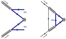
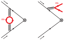
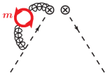
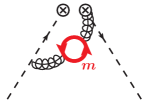
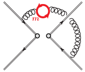
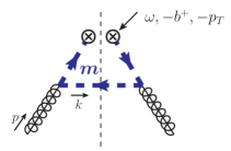
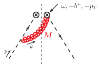
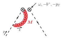
In general, one can distinguish two types of mass effects as illustrated in fig. 1, which have different characteristics: Contributions where the heavy-quark enters the hard interaction process are called primary mass effects. Contributions from a gluon splitting into a massive quark-antiquark pair with light quarks entering the hard interaction are called secondary. For the qTsubscript𝑞𝑇q_{T} spectrum, earlier treatments of the heavy-quark initiated primary contributions for mqTless-than-or-similar-to𝑚subscript𝑞𝑇m\lesssim q_{T} have been given in refs. Nadolsky:2002jr ; Berge:2005rv ; Belyaev:2005bs , essentially combining the ACOT scheme with the standard CSS qTsubscript𝑞𝑇q_{T} resummation. A complete setup also requires to account for secondary mass effects. Their systematic description for differential spectra in the various relevant hierarchies between mass and other physical scales has been established in the context of event shapes in e+esuperscript𝑒superscript𝑒e^{+}e^{-} collisions Gritschacher:2013pha ; Pietrulewicz:2014qza and for threshold resummation in DIS Hoang:2015iva , see also refs. Butenschoen:2016lpz ; Dehnadi:2016snl for a recent utilization in the context of boosted heavy quark initiated jets. The application to differential spectra in pp𝑝𝑝pp collisions will be part of the present paper.

We present a systematic effective-theory treatment of quark mass effects including both types of mass effects and all possible scale hierarchies using soft-collinear effective theory (SCET) Bauer:2000ew ; Bauer:2000yr ; Bauer:2001ct ; Bauer:2001yt . We focus on the Drell-Yan process, ppZ/γ+𝑝𝑝𝑍superscript𝛾superscriptsuperscriptpp\to Z/\gamma^{*}\to\ell^{+}\ell^{-}, and consider two types of observables that resolve additional QCD radiation and are used to constrain the process to the exclusive region, namely the transverse momentum qTsubscript𝑞𝑇q_{T} of the gauge boson and beam thrust Stewart:2009yx ,

qT=|qT|=|pT+pT¯|=|ipTi|,𝒯=imin{napi,nbpi}.formulae-sequencesubscript𝑞𝑇subscript𝑞𝑇subscript𝑝𝑇subscript𝑝𝑇¯subscript𝑖subscript𝑝𝑇𝑖𝒯subscript𝑖subscript𝑛𝑎subscript𝑝𝑖subscript𝑛𝑏subscript𝑝𝑖\displaystyle q_{T}=|\vec{q}_{T}|=\lvert\vec{p}_{T\ell}+\vec{p}_{T\bar{\ell}}\rvert=\Bigl{\lvert}\sum_{i}\vec{p}_{Ti}\Bigr{\rvert}\,,\qquad{\mathcal{T}}=\sum_{i}\min\{n_{a}\!\cdot\!p_{i},n_{b}\!\cdot\!p_{i}\}\,. (1)

Here, pisubscript𝑝𝑖p_{i} are all hadronic final-state momenta (i.e. excluding the color-singlet final state), and na,bμ=(1,±z^)superscriptsubscript𝑛𝑎𝑏𝜇1plus-or-minus^𝑧n_{a,b}^{\mu}=(1,\pm\hat{z}) are lightlike vectors along the beam axes. Due to transverse momentum conservation qTsubscript𝑞𝑇q_{T} measures the total transverse momentum of the final state hadronic radiation, while beam thrust measures the momentum projections of all hadronic particles onto the beam axis. The exclusive regime we are interested in corresponds to qTQmuch-less-thansubscript𝑞𝑇𝑄q_{T}\ll Q or 𝒯Qmuch-less-than𝒯𝑄{\mathcal{T}}\ll Q, where Q=q2𝑄superscript𝑞2Q=\sqrt{q^{2}} is the dilepton invariant mass. These two observables restrict the allowed QCD radiation into the collinear and soft regime in different ways, leading to different effective-theory setups with distinct factorization and resummation properties, which are well-known in the massless limit up to high orders in the logarithmic counting (see e.g. refs. Collins:1981uk ; Collins:1981va ; Collins:1984kg ; Balazs:1997xd ; Balazs:2000wv ; Bozzi:2010xn ; deFlorian:2011xf ; Becher:2010tm ; Chiu:2011qc ; Chiu:2012ir ; GarciaEchevarria:2011rb and refs. Stewart:2009yx ; Stewart:2010pd ; Berger:2010xi ). These two cases provide simple prototypical examples, which cover the essential features of the factorization with massive quarks that will also be relevant for including massive quark effects for other more complicated jet resolution variables whose factorization is known in the massless limit. Throughout the paper we always consider the limit ΛQCDqT,𝒯much-less-thansubscriptΛQCDsubscript𝑞𝑇𝒯\Lambda_{\mathrm{QCD}}\ll q_{T},{\mathcal{T}} allowing for a perturbative description of the physics at these kinematic scales. We then consider all relevant relative hierarchies between the heavy-quark mass m𝑚m and the kinematic scales set by the measurement of qTsubscript𝑞𝑇q_{T} or 𝒯𝒯{\mathcal{T}}, respectively.

Refer to caption
Refer to caption
Figure 1: Primary (a) and secondary (b) heavy-quark mass effects for Z𝑍Z-boson production.

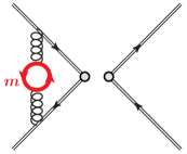
In the second part of the paper, we explicitly compute all required ingredients for incorporating mbsubscript𝑚𝑏m_{b} effects at NNLL order, which combines NNLL evolution with the full NNLO singular boundary conditions (hard, beam, and soft functions). For Z𝑍Z-boson production at NNLL, primary effects contribute via 𝒪(αs)×𝒪(αs)𝒪subscript𝛼𝑠𝒪subscript𝛼𝑠\mathcal{O}(\alpha_{s})\times\mathcal{O}(\alpha_{s}) heavy-quark initiated contributions, illustrated in fig. 1. Secondary effects contribute as 𝒪(αs2)𝒪superscriptsubscript𝛼𝑠2\mathcal{O}(\alpha_{s}^{2}) corrections to light-quark initiated hard interactions, illustrated in fig. 1. Due to the strong CKM suppression primary mbsubscript𝑚𝑏m_{b}-effects do not play any significant role for W𝑊W-production, which represents a key difference to Z𝑍Z-boson production. Primary mcsubscript𝑚𝑐m_{c}-effects enter W𝑊W-production in the (sizeable) cs𝑐𝑠cs-channel, where they start already at NLL via 𝒪(αs)×𝒪(1)𝒪subscript𝛼𝑠𝒪1\mathcal{O}(\alpha_{s})\times\mathcal{O}(1) corrections. For this case, our explicit results for the regime qTmcsimilar-tosubscript𝑞𝑇subscript𝑚𝑐q_{T}\sim m_{c} allows for up to NNLL resummation. (Here, the resummation at NNLL would require the 𝒪(αs2)𝒪superscriptsubscript𝛼𝑠2\mathcal{O}(\alpha_{s}^{2}) primary massive contributions.)

The paper is organized as follows: We first discuss in detail the effective field theory setup for the different parametric regimes for the case of qTsubscript𝑞𝑇q_{T} in sec. 2 and for 𝒯𝒯{\mathcal{T}} in sec. 3. Here, we elaborate on the relevant mode setup in SCET, the resulting factorization formulae, and all-order relations between the factorization ingredients in the different regimes. In sec. 4, we give the 𝒪(αs)𝒪subscript𝛼𝑠\mathcal{O}(\alpha_{s}) and 𝒪(αs2)𝒪superscriptsubscript𝛼𝑠2\mathcal{O}(\alpha_{s}^{2}) results for the various ingredients for NNLL resummation. We also verify the consistency of our results with the associated results in the massless limit. Further details on all calculations are given in the appendices, where we also give the analytic results at fixed-order for the massive quark effects in the qTsubscript𝑞𝑇q_{T} and 𝒯𝒯{\mathcal{T}} distributions in the singular limit qT,𝒯Qmuch-less-thansubscript𝑞𝑇𝒯𝑄q_{T},{\mathcal{T}}\ll Q. In sec. 5, we discuss the consequences of the secondary mass effects on the rapidity evolution, in particular for the qTsubscript𝑞𝑇q_{T} distribution in the regime qTmbsimilar-tosubscript𝑞𝑇subscript𝑚𝑏q_{T}\sim m_{b}. As an outlook we provide in sec. 6 an estimate of the potential size of the bottom quark effects for low-qTsubscript𝑞𝑇q_{T} Drell-Yan measurements. In sec. 7 we conclude.

2 Factorization of quark mass effects for the 𝒒𝑻subscript𝒒𝑻q_{T} spectrum

2.1 Factorization for massless quarks

Before discussing the massive quark corrections, we first briefly summarize the EFT setup and factorization for massless quarks. The relevant modes for the measurement of qTsubscript𝑞𝑇q_{T} in the limit qTQmuch-less-thansubscript𝑞𝑇𝑄q_{T}\ll Q are nasubscript𝑛𝑎n_{a}-collinear, nbsubscript𝑛𝑏n_{b}-collinear, and soft modes with the scaling

na-collinear:subscript𝑛𝑎-collinear:\displaystyle n_{a}\text{-collinear:} pnaμ(qT2Q,Q,qT),similar-tosuperscriptsubscript𝑝subscript𝑛𝑎𝜇superscriptsubscript𝑞𝑇2𝑄𝑄subscript𝑞𝑇\displaystyle\quad p_{n_{a}}^{\mu}\sim\Bigl{(}\frac{q_{T}^{2}}{Q},Q,q_{T}\Bigr{)}\,,
nb-collinear:subscript𝑛𝑏-collinear:\displaystyle n_{b}\text{-collinear:} pnbμ(Q,qT2Q,qT),similar-tosuperscriptsubscript𝑝subscript𝑛𝑏𝜇𝑄superscriptsubscript𝑞𝑇2𝑄subscript𝑞𝑇\displaystyle\quad p_{n_{b}}^{\mu}\sim\Bigl{(}Q,\frac{q_{T}^{2}}{Q},q_{T}\Bigr{)}\,,
soft: psμ(qT,qT,qT),similar-tosuperscriptsubscript𝑝𝑠𝜇subscript𝑞𝑇subscript𝑞𝑇subscript𝑞𝑇\displaystyle\quad p_{s}^{\mu}\sim(q_{T},q_{T},q_{T})\,, (2)

which we have written in terms of light-cone coordinates along the beam axis,

pμ=napnbμ2+nbpnaμ2+pμ(nap,nbp,p)(p+,p,p),superscript𝑝𝜇subscript𝑛𝑎𝑝superscriptsubscript𝑛𝑏𝜇2subscript𝑛𝑏𝑝superscriptsubscript𝑛𝑎𝜇2superscriptsubscript𝑝perpendicular-to𝜇subscript𝑛𝑎𝑝subscript𝑛𝑏𝑝subscript𝑝perpendicular-tosuperscript𝑝superscript𝑝subscript𝑝perpendicular-to\displaystyle p^{\mu}=n_{a}\!\cdot\!p\,\frac{n_{b}^{\mu}}{2}+n_{b}\!\cdot\!p\,\frac{n_{a}^{\mu}}{2}+p_{\perp}^{\mu}\equiv(n_{a}\!\cdot\!p,n_{b}\!\cdot\!p,p_{\perp})\equiv(p^{+},p^{-},p_{\perp})\,, (3)

with n¯anbsubscript¯𝑛𝑎subscript𝑛𝑏\bar{n}_{a}\equiv n_{b}. Besides these perturbative modes there are also nonperturbative collinear modes with the scaling (ΛQCD2/Q,Q,ΛQCD)superscriptsubscriptΛQCD2𝑄𝑄subscriptΛQCD(\Lambda_{\mathrm{QCD}}^{2}/Q,Q,\Lambda_{\mathrm{QCD}}) and (Q,ΛQCD2/Q,ΛQCD)𝑄superscriptsubscriptΛQCD2𝑄subscriptΛQCD(Q,\Lambda_{\mathrm{QCD}}^{2}/Q,\Lambda_{\mathrm{QCD}}), which describe the initial-state protons at the scale μΛQCDsimilar-to𝜇subscriptΛQCD\mu\sim\Lambda_{\mathrm{QCD}}, and which are unrelated to the specific jet resolution measurement. The typical invariant mass of the soft modes is parametrically the same as for the collinear modes, pna2pnb2ps2qT2similar-tosuperscriptsubscript𝑝subscript𝑛𝑎2superscriptsubscript𝑝subscript𝑛𝑏2similar-tosuperscriptsubscript𝑝𝑠2similar-tosuperscriptsubscript𝑞𝑇2p_{n_{a}}^{2}\sim p_{n_{b}}^{2}\sim p_{s}^{2}\sim q_{T}^{2}, which is the characteristic feature of a SCETIIsubscriptSCETII{\rm SCET}_{\rm II} theory. The soft and collinear modes are only separated in rapidity leading to the emergence of rapidity divergences and associated rapidity logarithms. The traditional approach for their resummation in QCD relies on the work by Collins, Soper, and Sterman Collins:1981uk ; Collins:1981va ; Collins:1984kg . In SCET the factorization and resummation were devised in refs. Becher:2010tm ; Chiu:2011qc ; Chiu:2012ir ; GarciaEchevarria:2011rb .

Here we will use the rapidity renormalization approach of refs. Chiu:2011qc ; Chiu:2012ir , where the rapidity divergences are regularized by a symmetric regulator and are renormalized by appropriate counterterms (by a MS¯¯MS\overline{\rm MS}-type subtraction). The rapidity logarithms are then resummed by solving the associated rapidity renormalization group equations. Within this framework the factorized differential cross section with nfsubscript𝑛𝑓n_{f} massless quarks reads111In principle there is also a corresponding contribution for a gluon initiated hard interaction. However, taking into account the decay of the electroweak boson into massless leptons this correction vanishes for onshell gluons and only contributes to the power suppressed terms of 𝒪(qT/Q)𝒪subscript𝑞𝑇𝑄\mathcal{O}(q_{T}/Q).

dσdqT2dQ2dYd𝜎dsubscriptsuperscript𝑞2𝑇dsuperscript𝑄2d𝑌\displaystyle\frac{\textrm{d}\sigma}{\textrm{d}q^{2}_{T}\,\textrm{d}Q^{2}\,\textrm{d}Y} =i,j{q,q¯}Hij(nf)(Q,μ)d2pTad2pTbd2pTsδ(qT2|pTa+pTb+pTs|2)absentsubscript𝑖𝑗𝑞¯𝑞subscriptsuperscript𝐻subscript𝑛𝑓𝑖𝑗𝑄𝜇superscriptd2subscript𝑝𝑇𝑎superscriptd2subscript𝑝𝑇𝑏superscriptd2subscript𝑝𝑇𝑠𝛿superscriptsubscript𝑞𝑇2superscriptsubscript𝑝𝑇𝑎subscript𝑝𝑇𝑏subscript𝑝𝑇𝑠2\displaystyle=\sum_{i,j\in\{q,\bar{q}\}}H^{(n_{f})}_{ij}(Q,\mu)\int\!\textrm{d}^{2}p_{Ta}\,\textrm{d}^{2}p_{Tb}\,\textrm{d}^{2}p_{Ts}\,\delta(q_{T}^{2}-|\vec{p}_{Ta}+\vec{p}_{Tb}+\vec{p}_{Ts}|^{2}) (4)
×Bi(nf)(pTa,xa,μ,νωa)Bj(nf)(pTb,xb,μ,νωb)S(nf)(pTs,μ,ν)[1+𝒪(qTQ)],absentsubscriptsuperscript𝐵subscript𝑛𝑓𝑖subscript𝑝𝑇𝑎subscript𝑥𝑎𝜇𝜈subscript𝜔𝑎subscriptsuperscript𝐵subscript𝑛𝑓𝑗subscript𝑝𝑇𝑏subscript𝑥𝑏𝜇𝜈subscript𝜔𝑏superscript𝑆subscript𝑛𝑓subscript𝑝𝑇𝑠𝜇𝜈delimited-[]1𝒪subscript𝑞𝑇𝑄\displaystyle\quad\times B^{(n_{f})}_{i}\Bigl{(}\vec{p}_{Ta},x_{a},\mu,\frac{\nu}{\omega_{a}}\Bigr{)}\,B^{(n_{f})}_{j}\Bigl{(}\vec{p}_{Tb},x_{b},\mu,\frac{\nu}{\omega_{b}}\Bigr{)}\,S^{(n_{f})}(\vec{p}_{Ts},\mu,\nu)\,\Bigl{[}1+\mathcal{O}\Bigl{(}\frac{q_{T}}{Q}\Bigr{)}\Bigr{]}\,,

where

ωa=QeY,ωb=QeY,xa,b=ωa,bEcm,formulae-sequencesubscript𝜔𝑎𝑄superscript𝑒𝑌formulae-sequencesubscript𝜔𝑏𝑄superscript𝑒𝑌subscript𝑥𝑎𝑏subscript𝜔𝑎𝑏subscript𝐸cm\displaystyle\omega_{a}=Qe^{Y}\,,\quad\omega_{b}=Qe^{-Y}\,,\quad x_{a,b}=\frac{\omega_{a,b}}{E_{\mathrm{cm}}}\,, (5)

with Y𝑌Y denoting the rapidity of the color-singlet state.

In eq. (4), the superscript (nf)subscript𝑛𝑓(n_{f}) on all functions indicates that the associated EFT operators and the strong coupling constant in these functions are renormalized with nfsubscript𝑛𝑓n_{f} active quark flavors, which matters for the evolution already at LL. Hijsubscript𝐻𝑖𝑗H_{ij} denotes the process-dependent (but measurement-independent) hard function. It encodes the tree-level result and hard virtual corrections of the partonic process ijZ/W/γ𝑖𝑗𝑍𝑊superscript𝛾ij\to Z/W/\gamma^{*} at the scale μQsimilar-to𝜇𝑄\mu\sim Q. Following refs. Collins:1981uw ; Fleming:2006cd ; Stewart:2009yx , the renormalized transverse-momentum dependent (TMD) beam functions Bisubscript𝐵𝑖B_{i}, which are essentially equivalent to TMDPDFs, can be matched onto PDFs as

Bi(nf)(pT,x,μ,νω)subscriptsuperscript𝐵subscript𝑛𝑓𝑖subscript𝑝𝑇𝑥𝜇𝜈𝜔\displaystyle B^{(n_{f})}_{i}\Bigl{(}\vec{p}_{T},x,\mu,\frac{\nu}{\omega}\Bigr{)} =kx1dzzik(nf)(pT,z,μ,νω)fk(nf)(xz,μ)[1+𝒪(ΛQCD2|pT|2)]absentsubscript𝑘superscriptsubscript𝑥1d𝑧𝑧subscriptsuperscriptsubscript𝑛𝑓𝑖𝑘subscript𝑝𝑇𝑧𝜇𝜈𝜔subscriptsuperscript𝑓subscript𝑛𝑓𝑘𝑥𝑧𝜇delimited-[]1𝒪superscriptsubscriptΛQCD2superscriptsubscript𝑝𝑇2\displaystyle=\sum_{k}\int_{x}^{1}\frac{\textrm{d}z}{z}\,\mathcal{I}^{(n_{f})}_{ik}\Bigl{(}\vec{p}_{T},z,\mu,\frac{\nu}{\omega}\Bigr{)}\,f^{(n_{f})}_{k}\Bigl{(}\frac{x}{z},\mu\Bigr{)}\biggl{[}1+\mathcal{O}\biggl{(}\frac{\Lambda_{\mathrm{QCD}}^{2}}{|\vec{p}_{T}|^{2}}\biggr{)}\biggr{]}
kik(nf)(pT,x,μ,νω)xfk(nf)(x,μ),absentsubscript𝑘subscripttensor-product𝑥subscriptsuperscriptsubscript𝑛𝑓𝑖𝑘subscript𝑝𝑇𝑥𝜇𝜈𝜔subscriptsuperscript𝑓subscript𝑛𝑓𝑘𝑥𝜇\displaystyle\equiv\sum_{k}\mathcal{I}^{(n_{f})}_{ik}(\vec{p}_{T},x,\mu,\frac{\nu}{\omega})\otimes_{x}f^{(n_{f})}_{k}(x,\mu)\,, (6)

where the perturbative matching coefficients iksubscript𝑖𝑘\mathcal{I}_{ik} describe the collinear initial-state radiation at the invariant mass scale μqTsimilar-to𝜇subscript𝑞𝑇\mu\sim q_{T} and rapidity scale νQsimilar-to𝜈𝑄\nu\sim Q, and the nonperturbative parton distribution functions (PDFs) are denoted by fksubscript𝑓𝑘f_{k}. In the following, we abbreviate the Mellin-type convolution in x𝑥x as in the second line above. Finally, the soft function S𝑆S describes the wide-angle soft radiation at the invariant mass and rapidity scale μνqTsimilar-to𝜇𝜈similar-tosubscript𝑞𝑇\mu\sim\nu\sim q_{T}. The matching coefficients iksubscript𝑖𝑘\mathcal{I}_{ik} and the soft function are process-independent and have been computed to 𝒪(αs2)𝒪superscriptsubscript𝛼𝑠2\mathcal{O}(\alpha_{s}^{2}) in refs. Catani:2012qa ; Gehrmann:2012ze ; Gehrmann:2014yya ; Luebbert:2016itl allowing for a full NNLL analysis of Drell-Yan for massless quarks. The three-loop noncusp rapidity anomalous dimension required for the resummation at N3LL has recently become available Li:2016axz ; Li:2016ctv ; Vladimirov:2016dll .

In eq. (4), the logarithms of qT/Qsubscript𝑞𝑇𝑄q_{T}/Q are resummed by evaluating all functions at their characteristic renormalization scales and evolving them to common final scales μ𝜇\mu and ν𝜈\nu by solving the set of coupled evolution equations

μddμHij(nf)(Q,μ)𝜇dd𝜇subscriptsuperscript𝐻subscript𝑛𝑓𝑖𝑗𝑄𝜇\displaystyle\mu\frac{\textrm{d}}{\textrm{d}\mu}H^{(n_{f})}_{ij}(Q,\mu) =γH(nf)(Q,μ)Hij(nf)(Q,μ),absentsuperscriptsubscript𝛾𝐻subscript𝑛𝑓𝑄𝜇subscriptsuperscript𝐻subscript𝑛𝑓𝑖𝑗𝑄𝜇\displaystyle=\gamma_{H}^{(n_{f})}(Q,\mu)\,H^{(n_{f})}_{ij}(Q,\mu)\,,
μddμBi(nf)(pT,x,μ,νω)𝜇dd𝜇subscriptsuperscript𝐵subscript𝑛𝑓𝑖subscript𝑝𝑇𝑥𝜇𝜈𝜔\displaystyle\mu\frac{\textrm{d}}{\textrm{d}\mu}B^{(n_{f})}_{i}\Bigl{(}\vec{p}_{T},x,\mu,\frac{\nu}{\omega}\Bigr{)} =γB(nf)(μ,νω)Bi(nf)(pT,x,μ,νω),absentsuperscriptsubscript𝛾𝐵subscript𝑛𝑓𝜇𝜈𝜔subscriptsuperscript𝐵subscript𝑛𝑓𝑖subscript𝑝𝑇𝑥𝜇𝜈𝜔\displaystyle=\gamma_{B}^{(n_{f})}\Bigl{(}\mu,\frac{\nu}{\omega}\Bigr{)}\,B^{(n_{f})}_{i}\Bigl{(}\vec{p}_{T},x,\mu,\frac{\nu}{\omega}\Bigr{)}\,,
μddμS(nf)(pT,μ,ν)𝜇dd𝜇superscript𝑆subscript𝑛𝑓subscript𝑝𝑇𝜇𝜈\displaystyle\mu\frac{\textrm{d}}{\textrm{d}\mu}S^{(n_{f})}(\vec{p}_{T},\mu,\nu) =γS(nf)(μ,ν)S(nf)(pT,μ,ν),absentsuperscriptsubscript𝛾𝑆subscript𝑛𝑓𝜇𝜈superscript𝑆subscript𝑛𝑓subscript𝑝𝑇𝜇𝜈\displaystyle=\gamma_{S}^{(n_{f})}(\mu,\nu)\,S^{(n_{f})}(\vec{p}_{T},\mu,\nu)\,,
μddμfi(nf)(x,μ)𝜇dd𝜇superscriptsubscript𝑓𝑖subscript𝑛𝑓𝑥𝜇\displaystyle\mu\frac{\textrm{d}}{\textrm{d}\mu}f_{i}^{(n_{f})}(x,\mu) =kγf,ik(nf)(x,μ)xfk(nf)(x,μ),absentsubscript𝑘subscripttensor-product𝑥superscriptsubscript𝛾𝑓𝑖𝑘subscript𝑛𝑓𝑥𝜇superscriptsubscript𝑓𝑘subscript𝑛𝑓𝑥𝜇\displaystyle=\sum_{k}\gamma_{f,ik}^{(n_{f})}(x,\mu)\otimes_{x}f_{k}^{(n_{f})}(x,\mu)\,,
νddνBi(nf)(pT,x,μ,νω)𝜈dd𝜈subscriptsuperscript𝐵subscript𝑛𝑓𝑖subscript𝑝𝑇𝑥𝜇𝜈𝜔\displaystyle\nu\frac{\textrm{d}}{\textrm{d}\nu}B^{(n_{f})}_{i}\Bigl{(}\vec{p}_{T},x,\mu,\frac{\nu}{\omega}\Bigr{)} =d2kTγν,B(nf)(pTkT,μ)Bi(nf)(kT,x,μ,νω),absentsuperscriptd2subscript𝑘𝑇superscriptsubscript𝛾𝜈𝐵subscript𝑛𝑓subscript𝑝𝑇subscript𝑘𝑇𝜇subscriptsuperscript𝐵subscript𝑛𝑓𝑖subscript𝑘𝑇𝑥𝜇𝜈𝜔\displaystyle=\int\!\textrm{d}^{2}k_{T}\,\gamma_{\nu,B}^{(n_{f})}(\vec{p}_{T}-\vec{k}_{T},\mu)\,B^{(n_{f})}_{i}\Bigl{(}\vec{k}_{T},x,\mu,\frac{\nu}{\omega}\Bigr{)}\,,
νddνS(nf)(pT,μ,ν)𝜈dd𝜈superscript𝑆subscript𝑛𝑓subscript𝑝𝑇𝜇𝜈\displaystyle\nu\frac{\textrm{d}}{\textrm{d}\nu}S^{(n_{f})}(\vec{p}_{T},\mu,\nu) =d2kTγν,S(nf)(pTkT,μ)S(nf)(kT,μ,ν).absentsuperscriptd2subscript𝑘𝑇superscriptsubscript𝛾𝜈𝑆subscript𝑛𝑓subscript𝑝𝑇subscript𝑘𝑇𝜇superscript𝑆subscript𝑛𝑓subscript𝑘𝑇𝜇𝜈\displaystyle=\int\!\textrm{d}^{2}k_{T}\,\gamma_{\nu,S}^{(n_{f})}(\vec{p}_{T}-\vec{k}_{T},\mu)\,S^{(n_{f})}(\vec{k}_{T},\mu,\nu)\,. (7)

Only the evolution of the PDF leads to flavor mixing. Consistency of RG running implies that

γH(nf)(Q,μ)+γB(nf)(μ,νωa)+γB(nf)(μ,νωb)+γS(nf)(μ,ν)superscriptsubscript𝛾𝐻subscript𝑛𝑓𝑄𝜇superscriptsubscript𝛾𝐵subscript𝑛𝑓𝜇𝜈subscript𝜔𝑎superscriptsubscript𝛾𝐵subscript𝑛𝑓𝜇𝜈subscript𝜔𝑏superscriptsubscript𝛾𝑆subscript𝑛𝑓𝜇𝜈\displaystyle\gamma_{H}^{(n_{f})}(Q,\mu)+\gamma_{B}^{(n_{f})}\Bigl{(}\mu,\frac{\nu}{\omega_{a}}\Bigr{)}+\gamma_{B}^{(n_{f})}\Bigl{(}\mu,\frac{\nu}{\omega_{b}}\Bigr{)}+\gamma_{S}^{(n_{f})}(\mu,\nu) =0,absent0\displaystyle=0\,,
2γν,B(nf)(pT,μ)+γν,S(nf)(pT,μ)2superscriptsubscript𝛾𝜈𝐵subscript𝑛𝑓subscript𝑝𝑇𝜇superscriptsubscript𝛾𝜈𝑆subscript𝑛𝑓subscript𝑝𝑇𝜇\displaystyle 2\gamma_{\nu,B}^{(n_{f})}(\vec{p}_{T},\mu)+\gamma_{\nu,S}^{(n_{f})}(\vec{p}_{T},\mu) =0,absent0\displaystyle=0\,,
μddμγν,S(nf)(pT,μ)=νddνγS(nf)(μ,ν)δ(pT)𝜇dd𝜇superscriptsubscript𝛾𝜈𝑆subscript𝑛𝑓subscript𝑝𝑇𝜇𝜈dd𝜈superscriptsubscript𝛾𝑆subscript𝑛𝑓𝜇𝜈𝛿subscript𝑝𝑇\displaystyle\mu\frac{\textrm{d}}{\textrm{d}\mu}\gamma_{\nu,S}^{(n_{f})}(\vec{p}_{T},\mu)=\nu\frac{\textrm{d}}{\textrm{d}\nu}\gamma_{S}^{(n_{f})}(\mu,\nu)\,\delta(\vec{p}_{T}) =4Γcusp(nf)[αs(μ)]δ(pT).absent4subscriptsuperscriptΓsubscript𝑛𝑓cuspdelimited-[]subscript𝛼𝑠𝜇𝛿subscript𝑝𝑇\displaystyle=-4\Gamma^{(n_{f})}_{\mathrm{cusp}}[\alpha_{s}(\mu)]\,\delta(\vec{p}_{T})\,. (8)

Note that in practice, the evolution is usually performed in Fourier space, such that one actually resums the conjugate logarithms ln(bμ)𝑏𝜇\ln(b\mu) where b=|bT|1/qT𝑏subscript𝑏𝑇similar-to1subscript𝑞𝑇b=\lvert\vec{b}_{T}\rvert\sim 1/q_{T} is the Fourier-conjugate variable to qTsubscript𝑞𝑇q_{T}. The qTsubscript𝑞𝑇q_{T} spectrum is then obtained as the inverse Fourier transform of the resummed b𝑏b-spectrum. The exact solution and evolution directly in qTsubscript𝑞𝑇q_{T} space, which directly resums the (distributional) logarithms in qTsubscript𝑞𝑇q_{T}, has been recently discussed in Ebert:2016gcn (see also ref. Monni:2016ktx ), and turns out to be significantly more involved due to the intrinsic two-dimensional nature of qTsubscript𝑞𝑇\vec{q}_{T}.

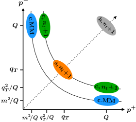
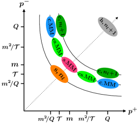
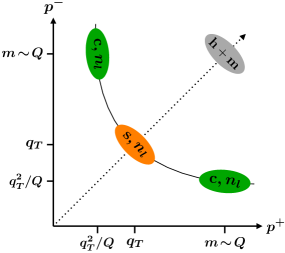
In the following subsections, we discuss how the mode and factorization setup changes when massive quark flavors are involved. These lead to the appearance of additional modes related to fluctuations around the mass shell as discussed extensively in refs. Gritschacher:2013pha ; Pietrulewicz:2014qza . For the different hierarchies between the mass scale m𝑚m and the scales Q𝑄Q and qTsubscript𝑞𝑇q_{T} the relevant modes are illustrated in fig. 2. In the first case, qTmQmuch-less-thansubscript𝑞𝑇𝑚similar-to𝑄q_{T}\ll m\sim Q, the massive flavor is integrated out at the hard scale, which leads to the above massless case with nlsubscript𝑛𝑙n_{l} massless flavors, as discussed in sec. 2.2. The second case, qTmQmuch-less-thansubscript𝑞𝑇𝑚much-less-than𝑄q_{T}\ll m\ll Q, where the quark mass is larger than the jet resolution variable, is analogous to the corresponding case for thrust in e+esuperscript𝑒superscript𝑒absente^{+}e^{-}\to dijets in refs. Gritschacher:2013pha ; Pietrulewicz:2014qza and DIS in the x1𝑥1x\to 1 limit Hoang:2015iva . We refer to these papers for details and only summarize briefly the main features for this regime in sec. 2.3. Our main focus is on the hierarchies qTmQsimilar-tosubscript𝑞𝑇𝑚much-less-than𝑄q_{T}\sim m\ll Q and mqTQmuch-less-than𝑚subscript𝑞𝑇much-less-than𝑄m\ll q_{T}\ll Q, which are important for bottom and charm quark mass effects at the LHC, and which are discussed in secs. 2.4 and 2.5.
Refer to caption
(a) qTmQmuch-less-thansubscript𝑞𝑇𝑚similar-to𝑄{q_{T}\ll m\sim Q}
Refer to caption
(b) qTmQmuch-less-thansubscript𝑞𝑇𝑚much-less-than𝑄{q_{T}\ll m\ll Q}
Refer to caption
(c) qTmQsimilar-tosubscript𝑞𝑇𝑚much-less-than𝑄{q_{T}\sim m\ll Q}
Refer to caption
(d) mqTQmuch-less-than𝑚subscript𝑞𝑇much-less-than𝑄{m\ll q_{T}\ll Q}
Figure 2: Effective theory modes for the qTsubscript𝑞𝑇q_{T} spectrum with massive quarks for qTQmuch-less-thansubscript𝑞𝑇𝑄q_{T}\ll Q and mΛQCDmuch-greater-than𝑚subscriptΛQCDm\gg\Lambda_{\rm QCD}.

2.2 Quark mass effects for mQsimilar-to𝑚𝑄m\sim Q

If the quark mass represents a large scale Qsimilar-toabsent𝑄\sim Q (which concerns the top quark at the LHC), this quark flavor does not play a dynamic role in the low-energy effective theory and is integrated out at the hard scale in the matching from QCD to SCET. The relevant modes are shown in fig. 2(a). The massive quark only contributes via mass-dependent contributions to the hard function. This yields the factorization theorem

dσdqT2dQ2dYd𝜎dsubscriptsuperscript𝑞2𝑇dsuperscript𝑄2d𝑌\displaystyle\frac{\textrm{d}\sigma}{\textrm{d}q^{2}_{T}\,\textrm{d}Q^{2}\,\textrm{d}Y} =i,j{q,q¯}Hij(Q,m,μ)d2pTad2pTbd2pTsδ(qT2|pTa+pTb+pTs|2)absentsubscript𝑖𝑗𝑞¯𝑞subscript𝐻𝑖𝑗𝑄𝑚𝜇superscriptd2subscript𝑝𝑇𝑎superscriptd2subscript𝑝𝑇𝑏superscriptd2subscript𝑝𝑇𝑠𝛿superscriptsubscript𝑞𝑇2superscriptsubscript𝑝𝑇𝑎subscript𝑝𝑇𝑏subscript𝑝𝑇𝑠2\displaystyle=\sum_{i,j\in\{q,\bar{q}\}}H_{ij}(Q,m,\mu)\,\int\textrm{d}^{2}p_{Ta}\,\textrm{d}^{2}p_{Tb}\,\textrm{d}^{2}p_{Ts}\,\delta(q_{T}^{2}-|\vec{p}_{Ta}+\vec{p}_{Tb}+\vec{p}_{Ts}|^{2}) (9)
×Bi(nl)(pTa,xa,μ,νωa)Bj(nl)(pTb,xb,μ,νωb)S(nl)(pTs,μ,ν)[1+𝒪(qT2m2,qTQ)],absentsubscriptsuperscript𝐵subscript𝑛𝑙𝑖subscript𝑝𝑇𝑎subscript𝑥𝑎𝜇𝜈subscript𝜔𝑎subscriptsuperscript𝐵subscript𝑛𝑙𝑗subscript𝑝𝑇𝑏subscript𝑥𝑏𝜇𝜈subscript𝜔𝑏superscript𝑆subscript𝑛𝑙subscript𝑝𝑇𝑠𝜇𝜈delimited-[]1𝒪superscriptsubscript𝑞𝑇2superscript𝑚2subscript𝑞𝑇𝑄\displaystyle\quad\times B^{(n_{l})}_{i}\Bigl{(}\vec{p}_{Ta},x_{a},\mu,\frac{\nu}{\omega_{a}}\Bigr{)}\,B^{(n_{l})}_{j}\Bigl{(}\vec{p}_{Tb},x_{b},\mu,\frac{\nu}{\omega_{b}}\Bigr{)}\,S^{(n_{l})}(\vec{p}_{Ts},\mu,\nu)\biggl{[}1+\mathcal{O}\Bigl{(}\frac{q_{T}^{2}}{m^{2}},\frac{q_{T}}{Q}\Bigr{)}\biggr{]}\,,

which is essentially equivalent to the massless case in the previous subsection with nlsubscript𝑛𝑙n_{l} massless flavors. The hard function Hij(Q,m,μ)subscript𝐻𝑖𝑗𝑄𝑚𝜇H_{ij}(Q,m,\mu) can be evaluated either in the (nf=nl)subscript𝑛𝑓subscript𝑛𝑙(n_{f}=n_{l}) or the (nf=nl+1)subscript𝑛𝑓subscript𝑛𝑙1(n_{f}=n_{l}+1) flavor scheme for αssubscript𝛼𝑠\alpha_{s}, where nlsubscript𝑛𝑙n_{l} is the number of light (massless) quark flavors. The associated massive quark corrections are directly related to the virtual contributions to the quark form factors, e.g. given at 𝒪(αs2)𝒪superscriptsubscript𝛼𝑠2\mathcal{O}(\alpha_{s}^{2}) by the virtual diagrams in fig. 1. In general both primary and secondary corrections contribute for initial (massless) quarks. Using the (nl)subscript𝑛𝑙(n_{l}) flavor scheme for αssubscript𝛼𝑠\alpha_{s} these vanish as 𝒪(Q2/m2)𝒪superscript𝑄2superscript𝑚2\mathcal{O}(Q^{2}/m^{2}) in the decoupling limit mQmuch-greater-than𝑚𝑄m\gg Q for the conserved vector current. For the axial-vector current, contributing to Z𝑍Z-boson production, there are in addition also anomaly corrections starting at 𝒪(αs2)𝒪superscriptsubscript𝛼𝑠2\mathcal{O}(\alpha_{s}^{2}) from the massive quark triangle in fig. 1 that do not decouple.222Instead, for mQmuch-greater-than𝑚𝑄m\gg Q the heavy quark can be integrated out around its mass scale and the axial current can be evolved between m𝑚m and Q𝑄Q to resum the associated logarithms ln(m/Q)𝑚𝑄\ln(m/Q). Since the massive quark does not appear as a dynamic flavor in the EFT below the hard scale Q𝑄Q, the entire RG evolution to sum the logarithms of qTsubscript𝑞𝑇q_{T} is performed with nlsubscript𝑛𝑙n_{l} massless flavors as in eq. (4).

2.3 Quark mass effects for qTmQmuch-less-thansubscript𝑞𝑇𝑚much-less-than𝑄q_{T}\ll m\ll Q

Next, we consider the hierarchies where the quark mass is parametrically smaller than the hard scale, mQmuch-less-than𝑚𝑄m\ll Q. These require a different factorization setup than mQsimilar-to𝑚𝑄m\sim Q since fluctuations around the mass-shell are now parametrically separated from hard fluctuations, which would lead to large unresummed logarithms inside the hard function Hij(Q,m,μ)subscript𝐻𝑖𝑗𝑄𝑚𝜇H_{ij}(Q,m,\mu). In this subsection, we start with the case where the transverse momentum is much smaller than the mass, qTmQmuch-less-thansubscript𝑞𝑇𝑚much-less-than𝑄q_{T}\ll m\ll Q, while qTmQsimilar-tosubscript𝑞𝑇𝑚much-less-than𝑄q_{T}\sim m\ll Q and mqTQmuch-less-than𝑚subscript𝑞𝑇much-less-than𝑄m\ll q_{T}\ll Q are considered in the following subsections.

In a first step the QCD current is matched onto the SCET current with nl+1subscript𝑛𝑙1n_{l}+1 dynamic quark flavors at the scale μQsimilar-to𝜇𝑄\mu\sim Q. Since mQmuch-less-than𝑚𝑄m\ll Q this matching can be performed (at leading order in the expansion parameter m/Q𝑚𝑄m/Q) only with massless quarks, leading to the hard function with nl+1subscript𝑛𝑙1n_{l}+1 massless flavors, Hij(nl+1)superscriptsubscript𝐻𝑖𝑗subscript𝑛𝑙1H_{ij}^{(n_{l}+1)}, with the strong coupling inside it renormalized with nl+1subscript𝑛𝑙1n_{l}+1 flavors. The matching is performed onto SCET containing nasubscript𝑛𝑎n_{a}-collinear, nbsubscript𝑛𝑏n_{b}-collinear, and soft mass modes with the scaling

na-collinear MM:subscript𝑛𝑎-collinear MM:\displaystyle n_{a}\text{-collinear MM:} pm,naμ(m2Q,Q,m),similar-tosuperscriptsubscript𝑝𝑚subscript𝑛𝑎𝜇superscript𝑚2𝑄𝑄𝑚\displaystyle\quad p_{m,n_{a}}^{\mu}\sim\Bigl{(}\frac{m^{2}}{Q},Q,m\Bigr{)}\,,
nb-collinear MM:subscript𝑛𝑏-collinear MM:\displaystyle n_{b}\text{-collinear MM:} pm,nbμ(Q,m2Q,m),similar-tosuperscriptsubscript𝑝𝑚subscript𝑛𝑏𝜇𝑄superscript𝑚2𝑄𝑚\displaystyle\quad p_{m,n_{b}}^{\mu}\sim\Bigl{(}Q,\frac{m^{2}}{Q},m\Bigr{)}\,,
soft MM: pm,sμ(m,m,m),similar-tosuperscriptsubscript𝑝𝑚𝑠𝜇𝑚𝑚𝑚\displaystyle\quad p_{m,s}^{\mu}\sim(m,m,m)\,, (10)

as illustrated in fig. 2(b). These mass-shell fluctuations arise here purely from secondary virtual contributions.

In a second step at the scale μmsimilar-to𝜇𝑚\mu\sim m, the mass modes are integrated out and the SCET with nlsubscript𝑛𝑙n_{l} massless and one massive flavor is matched onto SCET with nlsubscript𝑛𝑙n_{l} massless flavors with the usual scaling as in the massless case in eq. (2.1). Since the soft and collinear mass modes have the same invariant mass set by the quark mass and are only separated in rapidity, there are rapidity divergences in their (unrenormalized) collinear and soft contributions. Their renormalization and the resummation of the associated logarithms can be again handled using the rapidity RG approach in refs. Chiu:2011qc ; Chiu:2012ir , which has been explicitly carried out in ref. Hoang:2015vua .333The matching in ref. Hoang:2015vua was performed with massive primary quarks yielding the matching functions denoted as Hm,nsubscript𝐻𝑚𝑛H_{m,n}, Hm,n¯subscript𝐻𝑚¯𝑛H_{m,\bar{n}} and Hm,ssubscript𝐻𝑚𝑠H_{m,s} there. However, this does not affect the structure of the rapidity logarithms arising from the secondary mass effects, which are independent of the primary quarks being massive or massless. In addition, all renormalized parameters like the strong coupling constant are matched at the mass scale from nl+1subscript𝑛𝑙1n_{l}+1 to nlsubscript𝑛𝑙n_{l} flavors taking into account that the massive flavor is removed as a dynamic degree of freedom.

After these steps, the factorization at the low scale qTsimilar-toabsentsubscript𝑞𝑇\sim q_{T} proceeds as in the massless case with all operator matrix elements depending on the nlsubscript𝑛𝑙n_{l} massless flavors, which yields the factorization theorem

dσdqT2dQ2dYd𝜎dsubscriptsuperscript𝑞2𝑇dsuperscript𝑄2d𝑌\displaystyle\frac{\textrm{d}\sigma}{\textrm{d}q^{2}_{T}\,\textrm{d}Q^{2}\,\textrm{d}Y} =i,j{q,q¯}Hij(nl+1)(Q,μ)Hc(m,μ,νωa)Hc(m,μ,νωb)Hs(m,μ,ν)absentsubscript𝑖𝑗𝑞¯𝑞subscriptsuperscript𝐻subscript𝑛𝑙1𝑖𝑗𝑄𝜇subscript𝐻𝑐𝑚𝜇𝜈subscript𝜔𝑎subscript𝐻𝑐𝑚𝜇𝜈subscript𝜔𝑏subscript𝐻𝑠𝑚𝜇𝜈\displaystyle=\sum_{i,j\in\{q,\bar{q}\}}H^{(n_{l}+1)}_{ij}(Q,\mu)\,H_{c}\Bigl{(}m,\mu,\frac{\nu}{\omega_{a}}\Bigr{)}H_{c}\Bigl{(}m,\mu,\frac{\nu}{\omega_{b}}\Bigr{)}H_{s}(m,\mu,\nu)
×d2pTad2pTbd2pTsδ(qT2|pTa+pTb+pTs|2)Bi(nl)(pTa,xa,μ,νωa)\displaystyle\quad\times\int\textrm{d}^{2}p_{Ta}\,\textrm{d}^{2}p_{Tb}\,\textrm{d}^{2}p_{Ts}\,\delta(q_{T}^{2}-|\vec{p}_{Ta}+\vec{p}_{Tb}+\vec{p}_{Ts}|^{2})\,B^{(n_{l})}_{i}\Bigl{(}\vec{p}_{Ta},x_{a},\mu,\frac{\nu}{\omega_{a}}\Bigr{)}
×Bj(nl)(pTb,xb,μ,νωb)S(nl)(pTs,μ,ν)[1+𝒪(qTQ,qT2m2,m2Q2)].absentsubscriptsuperscript𝐵subscript𝑛𝑙𝑗subscript𝑝𝑇𝑏subscript𝑥𝑏𝜇𝜈subscript𝜔𝑏superscript𝑆subscript𝑛𝑙subscript𝑝𝑇𝑠𝜇𝜈delimited-[]1𝒪subscript𝑞𝑇𝑄superscriptsubscript𝑞𝑇2superscript𝑚2superscript𝑚2superscript𝑄2\displaystyle\quad\times B^{(n_{l})}_{j}\Bigl{(}\vec{p}_{Tb},x_{b},\mu,\frac{\nu}{\omega_{b}}\Bigr{)}\,S^{(n_{l})}(\vec{p}_{Ts},\mu,\nu)\,\Bigl{[}1+\mathcal{O}\Bigl{(}\frac{q_{T}}{Q},\frac{q_{T}^{2}}{m^{2}},\frac{m^{2}}{Q^{2}}\Bigr{)}\Bigr{]}\,. (11)

Here Hcsubscript𝐻𝑐H_{c} and Hssubscript𝐻𝑠H_{s} denote the hard functions that arise from the matching at the mass scale μmsimilar-to𝜇𝑚\mu\sim m. Their natural rapidity scales are νQsimilar-to𝜈𝑄\nu\sim Q for the collinear contributions and νmsimilar-to𝜈𝑚\nu\sim m for the soft ones. They can be evaluated in either the (nl)subscript𝑛𝑙(n_{l}) or (nl+1)subscript𝑛𝑙1(n_{l}+1) scheme for αssubscript𝛼𝑠\alpha_{s}. We will give their expressions at 𝒪(αs2)𝒪superscriptsubscript𝛼𝑠2\mathcal{O}(\alpha_{s}^{2}) in sec. 4.1. The resummation of all logarithms of ratios of qTsubscript𝑞𝑇q_{T}, m𝑚m, and Q𝑄Q is achieved by performing the evolution in μ𝜇\mu and ν𝜈\nu of all functions appearing in eq. (2.3) from their natural scales.

In principle, the μ𝜇\mu evolution can be performed by evolving all functions with their respective number of quark flavors without switching the flavor scheme, i.e. with nl+1subscript𝑛𝑙1n_{l}+1 flavors for H𝐻H, nlsubscript𝑛𝑙n_{l} flavors for B𝐵B and S𝑆S and an additional evolution for the collinear and soft matching functions Hcsubscript𝐻𝑐H_{c} and Hssubscript𝐻𝑠H_{s}. The consistency of RG running for the factorization theorems in eqs. (2.3) and (9), and eq. (2.1) with nlsubscript𝑛𝑙n_{l} massless flavors, implies that the μ𝜇\mu-dependence of the mass-dependent hard functions Hcsubscript𝐻𝑐H_{c} and Hssubscript𝐻𝑠H_{s} is precisely given by the difference between nlsubscript𝑛𝑙n_{l} and nl+1subscript𝑛𝑙1n_{l}+1 active quark flavors in the evolution of the hard function Hijsubscript𝐻𝑖𝑗H_{ij},

γHc(m,μ,νωa)+γHc(m,μ,νωb)+γHs(m,μ,ν)=γH(nl)(Q,μ)γH(nl+1)(Q,μ),subscript𝛾subscript𝐻𝑐𝑚𝜇𝜈subscript𝜔𝑎subscript𝛾subscript𝐻𝑐𝑚𝜇𝜈subscript𝜔𝑏subscript𝛾subscript𝐻𝑠𝑚𝜇𝜈subscriptsuperscript𝛾subscript𝑛𝑙𝐻𝑄𝜇subscriptsuperscript𝛾subscript𝑛𝑙1𝐻𝑄𝜇\displaystyle\gamma_{H_{c}}\Bigl{(}m,\mu,\frac{\nu}{\omega_{a}}\Bigr{)}+\gamma_{H_{c}}\Bigl{(}m,\mu,\frac{\nu}{\omega_{b}}\Bigr{)}+\gamma_{H_{s}}(m,\mu,\nu)=\gamma^{(n_{l})}_{H}(Q,\mu)-\gamma^{(n_{l}+1)}_{H}(Q,\mu)\,, (12)

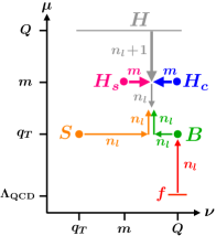
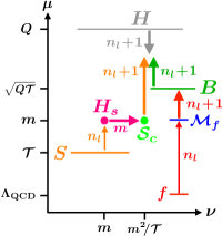
where γH(nf)subscriptsuperscript𝛾subscript𝑛𝑓𝐻\gamma^{(n_{f})}_{H} is defined in eq. (2.1), and γHcsubscript𝛾subscript𝐻𝑐\gamma_{H_{c}} and γHssubscript𝛾subscript𝐻𝑠\gamma_{H_{s}} are defined analogously. At two loops this relation can be checked explicitly using the results in eqs. (4.1.2), (4.1.2) and (A.1). As a result, the μ𝜇\mu evolution for the hard functions can be conveniently implemented as illustrated in fig. 3(a), by carrying out the μ𝜇\mu evolution with nlsubscript𝑛𝑙n_{l} active quark flavors below the matching scale μmmsimilar-tosubscript𝜇𝑚𝑚\mu_{m}\sim m and with nl+1subscript𝑛𝑙1n_{l}+1 flavors above μmsubscript𝜇𝑚\mu_{m}, providing in this sense a “variable-flavor number scheme” Pietrulewicz:2014qza ; Hoang:2015iva . (This effectively corresponds to using operator running for the hard scattering current, which is renormalized with nl+1subscript𝑛𝑙1n_{l}+1 flavors above the mass scale and with nlsubscript𝑛𝑙n_{l} flavors below the mass scale.) In addition there is also a rapidity evolution, which is carried out at μm=msubscript𝜇𝑚𝑚\mu_{m}=m, i.e. at the border between the (nl+1)subscript𝑛𝑙1(n_{l}+1) and (nl)subscript𝑛𝑙(n_{l})-flavor theories (see ref. Hoang:2015vua ), which is governed by the mass-dependent rapidity anomalous dimensions for Hssubscript𝐻𝑠H_{s} and Hcsubscript𝐻𝑐H_{c},

γν,Hs(m,μ)=2γν,Hc(m,μ)=ddlnνlnHs(m,μ,ν).subscript𝛾𝜈subscript𝐻𝑠𝑚𝜇2subscript𝛾𝜈subscript𝐻𝑐𝑚𝜇dd𝜈subscript𝐻𝑠𝑚𝜇𝜈\displaystyle\gamma_{\nu,H_{s}}(m,\mu)=-2\gamma_{\nu,H_{c}}(m,\mu)=\frac{\textrm{d}}{\textrm{d}\ln\nu}\ln H_{s}(m,\mu,\nu)\,. (13)
Refer to caption
(a) qTmQmuch-less-thansubscript𝑞𝑇𝑚much-less-than𝑄{q_{T}\ll m\ll Q}
Refer to caption
(b) qTmQsimilar-tosubscript𝑞𝑇𝑚much-less-than𝑄{q_{T}\sim m\ll Q}
Refer to caption
(c) mqTQmuch-less-than𝑚subscript𝑞𝑇much-less-than𝑄{m\ll q_{T}\ll Q}
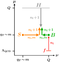
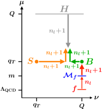
Figure 3: Illustration of the renormalization group evolution for qTsubscript𝑞𝑇q_{T} of the hard, beam, soft, and parton distribution functions in invariant mass and rapidity. The anomalous dimensions for each evolution step involve the displayed number of active quark flavors. The label m𝑚m indicates that the corresponding evolution is mass dependent.

2.4 Quark mass effects for qTmQsimilar-tosubscript𝑞𝑇𝑚much-less-than𝑄q_{T}\sim m\ll Q

If the qTsubscript𝑞𝑇q_{T} scale is of the order of the quark mass, qTmsimilar-tosubscript𝑞𝑇𝑚q_{T}\sim m, the massive quark becomes a dynamic degree of freedom, which contributes to the qTsubscript𝑞𝑇q_{T} spectrum via real radiation effects. The mass modes in eq. (2.3) are now the same as the usual massless SCETIIsubscriptSCETII{\rm SCET}_{\rm II} modes for the qTsubscript𝑞𝑇q_{T} measurement in eq. (2.1), since their parametrically scaling coincides for qTmsimilar-tosubscript𝑞𝑇𝑚q_{T}\sim m, as illustrated in fig. 2(c). In this case, there is only a single matching at the hard scale μQsimilar-to𝜇𝑄\mu\sim Q from QCD onto SCET with these common soft and collinear modes. This hard matching gives again rise to the (mass-independent) hard function Hij(nl+1)superscriptsubscript𝐻𝑖𝑗subscript𝑛𝑙1H_{ij}^{(n_{l}+1)} for nl+1subscript𝑛𝑙1n_{l}+1 massless flavors. The SCET operator matrix elements at the scale μqTsimilar-to𝜇subscript𝑞𝑇\mu\sim q_{T}, i.e. the beam and soft functions, now encode the effects of the massive quark. They are now renormalized with nl+1subscript𝑛𝑙1n_{l}+1 quark flavors and contain an explicit dependence on the quark mass. When integrating out the modes with the virtuality qTsubscript𝑞𝑇q_{T} also the massive quark is integrated out and the collinear matching functions iksubscript𝑖𝑘\mathcal{I}_{ik} between the beam functions and the PDFs thus also contain the effect from changing from nl+1subscript𝑛𝑙1n_{l}+1 to nlsubscript𝑛𝑙n_{l} flavors, i.e.

Bi(nl+1)(pT,m,x,μ,νω)=k{q,q¯,g}ik(pT,m,x,μ,νω)xfk(nl)(x,μ)[1+𝒪(ΛQCD2m2,ΛQCD2qT2)].superscriptsubscript𝐵𝑖subscript𝑛𝑙1subscript𝑝𝑇𝑚𝑥𝜇𝜈𝜔subscript𝑘𝑞¯𝑞𝑔subscripttensor-product𝑥subscript𝑖𝑘subscript𝑝𝑇𝑚𝑥𝜇𝜈𝜔subscriptsuperscript𝑓subscript𝑛𝑙𝑘𝑥𝜇delimited-[]1𝒪superscriptsubscriptΛQCD2superscript𝑚2superscriptsubscriptΛQCD2superscriptsubscript𝑞𝑇2\displaystyle B_{i}^{(n_{l}+1)}\Bigl{(}\vec{p}_{T},m,x,\mu,\frac{\nu}{\omega}\Bigr{)}=\sum_{k\in\{q,\bar{q},g\}}\mathcal{I}_{ik}\Bigl{(}\vec{p}_{T},m,x,\mu,\frac{\nu}{\omega}\Bigr{)}\otimes_{x}f^{(n_{l})}_{k}(x,\mu)\Bigl{[}1+\mathcal{O}\Bigl{(}\frac{\Lambda_{\mathrm{QCD}}^{2}}{m^{2}},\frac{\Lambda_{\mathrm{QCD}}^{2}}{q_{T}^{2}}\Bigr{)}\Bigr{]}\,. (14)

Written out explicitly, the factorization theorem reads

dσdqT2dQ2dYd𝜎dsubscriptsuperscript𝑞2𝑇dsuperscript𝑄2d𝑌\displaystyle\frac{\textrm{d}\sigma}{\textrm{d}q^{2}_{T}\,\textrm{d}Q^{2}\,\textrm{d}Y} =i,j{q,q¯,Q,Q¯}Hij(nl+1)(Q,μ)d2pTad2pTbd2pTsδ(qT2|pTa+pTb+pTs|2)absentsubscript𝑖𝑗𝑞¯𝑞𝑄¯𝑄subscriptsuperscript𝐻subscript𝑛𝑙1𝑖𝑗𝑄𝜇superscriptd2subscript𝑝𝑇𝑎superscriptd2subscript𝑝𝑇𝑏superscriptd2subscript𝑝𝑇𝑠𝛿superscriptsubscript𝑞𝑇2superscriptsubscript𝑝𝑇𝑎subscript𝑝𝑇𝑏subscript𝑝𝑇𝑠2\displaystyle=\sum_{i,j\in\{q,\bar{q},Q,\bar{Q}\}}H^{(n_{l}+1)}_{ij}(Q,\mu)\,\int\textrm{d}^{2}p_{Ta}\,\textrm{d}^{2}p_{Tb}\,\textrm{d}^{2}p_{Ts}\,\delta(q_{T}^{2}-|\vec{p}_{Ta}+\vec{p}_{Tb}+\vec{p}_{Ts}|^{2})
×[k{q,q¯,g}ik(pTa,m,xa,μ,νωa)xfk(nl)(xa,μ)]absentdelimited-[]subscript𝑘𝑞¯𝑞𝑔subscripttensor-product𝑥subscript𝑖𝑘subscript𝑝𝑇𝑎𝑚subscript𝑥𝑎𝜇𝜈subscript𝜔𝑎subscriptsuperscript𝑓subscript𝑛𝑙𝑘subscript𝑥𝑎𝜇\displaystyle\quad\times\biggl{[}\sum_{k\in\{q,\bar{q},g\}}\mathcal{I}_{ik}\Bigl{(}\vec{p}_{Ta},m,x_{a},\mu,\frac{\nu}{\omega_{a}}\Bigr{)}\otimes_{x}f^{(n_{l})}_{k}(x_{a},\mu)\biggr{]}
×[k{q,q¯,g}jk(pTb,m,xb,μ,νωb)xfk(nl)(xb,μ)]absentdelimited-[]subscript𝑘𝑞¯𝑞𝑔subscripttensor-product𝑥subscript𝑗𝑘subscript𝑝𝑇𝑏𝑚subscript𝑥𝑏𝜇𝜈subscript𝜔𝑏subscriptsuperscript𝑓subscript𝑛𝑙𝑘subscript𝑥𝑏𝜇\displaystyle\quad\times\biggl{[}\sum_{k\in\{q,\bar{q},g\}}\mathcal{I}_{jk}\Bigl{(}\vec{p}_{Tb},m,x_{b},\mu,\frac{\nu}{\omega_{b}}\Bigr{)}\otimes_{x}f^{(n_{l})}_{k}(x_{b},\mu)\biggr{]}
×S(pTs,m,μ,ν)[1+𝒪(qTQ,m2Q2,ΛQCD2m2,ΛQCD2qT2)],absent𝑆subscript𝑝𝑇𝑠𝑚𝜇𝜈delimited-[]1𝒪subscript𝑞𝑇𝑄superscript𝑚2superscript𝑄2superscriptsubscriptΛQCD2superscript𝑚2superscriptsubscriptΛQCD2superscriptsubscript𝑞𝑇2\displaystyle\quad\times S(\vec{p}_{Ts},m,\mu,\nu)\,\biggl{[}1+\mathcal{O}\Bigl{(}\frac{q_{T}}{Q},\frac{m^{2}}{Q^{2}},\frac{\Lambda_{\mathrm{QCD}}^{2}}{m^{2}},\frac{\Lambda_{\mathrm{QCD}}^{2}}{q_{T}^{2}}\Bigr{)}\biggr{]}\,, (15)

where i,j=Q,Q¯formulae-sequence𝑖𝑗𝑄¯𝑄i,j=Q,\bar{Q} denotes the massive quark flavor in the sum over flavors. We stress that the renormalization of the bare soft and beam function with nlsubscript𝑛𝑙n_{l} massless and one massive flavor is carried out in the nl+1subscript𝑛𝑙1n_{l}+1 flavor scheme for αssubscript𝛼𝑠\alpha_{s}, while the strong coupling in the PDFs (which are defined in the lower theory with nlsubscript𝑛𝑙n_{l} massless flavors) is renormalized with nlsubscript𝑛𝑙n_{l} flavors. The renormalized soft function and beam function coefficients iksubscript𝑖𝑘\mathcal{I}_{ik} can then be expressed in terms of either the (nl+1)subscript𝑛𝑙1(n_{l}+1) or the (nl)subscript𝑛𝑙(n_{l}) flavor scheme for αssubscript𝛼𝑠\alpha_{s} without introducing large logarithms.

In this hierarchy quark mass effects enter in eq. (2.4) at 𝒪(αs2)𝒪superscriptsubscript𝛼𝑠2\mathcal{O}(\alpha_{s}^{2}) in two ways: There are secondary radiation effects appearing in the two-loop soft function S(2)superscript𝑆2S^{(2)} and the flavor-diagonal beam function matching coefficients qq(2)subscriptsuperscript2𝑞𝑞\mathcal{I}^{(2)}_{qq}. In addition, there are primary mass effects arising from a massive-quark initiated hard process. For Z/γ𝑍superscript𝛾Z/\gamma^{*} production, this requires the production of the massive quarks via gluon splitting in both collinear sectors, which manifests itself in two one-loop collinear matching coefficients Qg(1)×Q¯g(1)subscriptsuperscript1𝑄𝑔subscriptsuperscript1¯𝑄𝑔\mathcal{I}^{(1)}_{Qg}\times\mathcal{I}^{(1)}_{\bar{Q}g}. For W𝑊W-boson production, primary charm quark effects enter already at 𝒪(αs)𝒪subscript𝛼𝑠\mathcal{O}(\alpha_{s}) from a single Qg(1)subscriptsuperscript1𝑄𝑔\mathcal{I}^{(1)}_{Qg} with Q=c𝑄𝑐Q=c.

The resummation of logarithms ln(qT/Q)subscript𝑞𝑇𝑄\ln(q_{T}/Q) and ln(m/Q)𝑚𝑄\ln(m/Q) is again obtained by performing the RG evolution for eq. (2.4), which is illustrated in fig. 3(b). While the evolution of the PDFs proceeds in nlsubscript𝑛𝑙n_{l} flavors, the μ𝜇\mu-evolution for the hard, beam, and soft functions above the scale m𝑚m is now carried out purely with nl+1subscript𝑛𝑙1n_{l}+1 flavors. Consistency of RG running for eq. (14) implies that the matching coefficients iksubscript𝑖𝑘\mathcal{I}_{ik} satisfy

μddμik(pT,m,z,μ,νω)𝜇dd𝜇subscript𝑖𝑘subscript𝑝𝑇𝑚𝑧𝜇𝜈𝜔\displaystyle\mu\frac{\textrm{d}}{\textrm{d}\mu}\,\mathcal{I}_{ik}\Bigl{(}\vec{p}_{T},m,z,\mu,\frac{\nu}{\omega}\Bigr{)} =[γBi(nl+1)×ik](pT,m,z,μ,νω)jq,q¯,g[ijγf,jk(nl)](pT,m,z,μ,νω).absentdelimited-[]subscriptsuperscript𝛾subscript𝑛𝑙1subscript𝐵𝑖subscript𝑖𝑘subscript𝑝𝑇𝑚𝑧𝜇𝜈𝜔subscript𝑗𝑞¯𝑞𝑔delimited-[]tensor-productsubscript𝑖𝑗subscriptsuperscript𝛾subscript𝑛𝑙𝑓𝑗𝑘subscript𝑝𝑇𝑚𝑧𝜇𝜈𝜔\displaystyle=\Bigl{[}\gamma^{(n_{l}+1)}_{B_{i}}\times\mathcal{I}_{ik}\Bigr{]}\Bigl{(}\vec{p}_{T},m,z,\mu,\frac{\nu}{\omega}\Bigr{)}-\sum_{j\in q,\bar{q},g}\Bigl{[}\mathcal{I}_{ij}\otimes\gamma^{(n_{l})}_{f,jk}\Bigr{]}\Bigl{(}\vec{p}_{T},m,z,\mu,\frac{\nu}{\omega}\Bigr{)}\,. (16)

Since the renormalization of the beam functions does not involve parton mixing, the one-loop primary mass contributions to Qg(1)superscriptsubscript𝑄𝑔1{\mathcal{I}}_{Qg}^{(1)} cannot give rise to rapidity divergences and associated logarithms. On the other hand, the secondary mass effects change the rapidity evolution. In particular, the beam and soft ν𝜈\nu-anomalous dimensions become mass dependent444The fact that quark masses can affect the evolution was already pointed out in ref. Collins:1984kg .,

νddνBi(nl+1)(pT,m,μ,νω)𝜈dd𝜈superscriptsubscript𝐵𝑖subscript𝑛𝑙1subscript𝑝𝑇𝑚𝜇𝜈𝜔\displaystyle\nu\frac{\textrm{d}}{\textrm{d}\nu}B_{i}^{(n_{l}+1)}\Bigl{(}\vec{p}_{T},m,\mu,\frac{\nu}{\omega}\Bigr{)} =d2kTγν,B(nl+1)(pTkT,m,μ)Bi(nl+1)(kT,m,μ,νω),absentsuperscriptd2subscript𝑘𝑇subscriptsuperscript𝛾subscript𝑛𝑙1𝜈𝐵subscript𝑝𝑇subscript𝑘𝑇𝑚𝜇superscriptsubscript𝐵𝑖subscript𝑛𝑙1subscript𝑘𝑇𝑚𝜇𝜈𝜔\displaystyle=\int\!\textrm{d}^{2}k_{T}\,\gamma^{(n_{l}+1)}_{\nu,B}(\vec{p}_{T}-\vec{k}_{T},m,\mu)\,B_{i}^{(n_{l}+1)}\Bigl{(}\vec{k}_{T},m,\mu,\frac{\nu}{\omega}\Bigr{)}\,,
νddνS(nl+1)(pT,m,μ,ν)𝜈dd𝜈superscript𝑆subscript𝑛𝑙1subscript𝑝𝑇𝑚𝜇𝜈\displaystyle\nu\frac{\textrm{d}}{\textrm{d}\nu}S^{(n_{l}+1)}(\vec{p}_{T},m,\mu,\nu) =d2kTγν,S(nl+1)(pTkT,m,μ)S(nl+1)(kT,m,μ,ν).absentsuperscriptd2subscript𝑘𝑇subscriptsuperscript𝛾subscript𝑛𝑙1𝜈𝑆subscript𝑝𝑇subscript𝑘𝑇𝑚𝜇superscript𝑆subscript𝑛𝑙1subscript𝑘𝑇𝑚𝜇𝜈\displaystyle=\int\!\textrm{d}^{2}k_{T}\,\gamma^{(n_{l}+1)}_{\nu,S}(\vec{p}_{T}-\vec{k}_{T},m,\mu)\,S^{(n_{l}+1)}(\vec{k}_{T},m,\mu,\nu)\,. (17)

We discuss the implications of the mass dependence for the rapidity evolution in sec. 5.

2.5 Quark mass effects for mqTQmuch-less-than𝑚subscript𝑞𝑇much-less-than𝑄m\ll q_{T}\ll Q

If qTsubscript𝑞𝑇q_{T} is much larger than the mass, the fluctuations around the mass-shell take place at a different scale than the jet resolution measurement. There are no relevant soft fluctuations scaling like pm,sμ(m,m,m)similar-tosuperscriptsubscript𝑝𝑚𝑠𝜇𝑚𝑚𝑚p_{m,s}^{\mu}\sim(m,m,m), since the measurement of qTsubscript𝑞𝑇q_{T} is IR safe and is thus insensitive to the lower mass scale. (In other words, if we were to explicitly distinguish such soft mass modes their contribution would cancel as for an inclusive observable since they are not constrained by the qTsubscript𝑞𝑇q_{T}-measurement.) This means that the soft modes are described by a soft function with nl+1subscript𝑛𝑙1n_{l}+1 massless flavors at the scale μqTsimilar-to𝜇subscript𝑞𝑇\mu\sim q_{T}. Due to the collinear sensitivity of the initial-state radiation there are still relevant collinear mass modes scaling like pm,naμ(m2/Q,Q,m)similar-tosuperscriptsubscript𝑝𝑚subscript𝑛𝑎𝜇superscript𝑚2𝑄𝑄𝑚p_{m,n_{a}}^{\mu}\sim(m^{2}/Q,Q,m) and pm,nbμ(Q,m2/Q,m)similar-tosuperscriptsubscript𝑝𝑚subscript𝑛𝑏𝜇𝑄superscript𝑚2𝑄𝑚p_{m,n_{b}}^{\mu}\sim(Q,m^{2}/Q,m), as illustrated in fig. 2(d). Thus there are collinear modes in SCET at different invariant mass scales, which can be disentangled by a multistage matching. First, the beam functions are matched onto the PDFs with nlsubscript𝑛𝑙n_{l} massless and one massive flavor. Since this matching takes place at the scale μBqTmsimilar-tosubscript𝜇𝐵subscript𝑞𝑇much-greater-than𝑚\mu_{B}\sim q_{T}\gg m this gives just the matching coefficients iksubscript𝑖𝑘\mathcal{I}_{ik} for nl+1subscript𝑛𝑙1n_{l}+1 massless flavors,

Bi(nl+1)(pT,m,x,μ,νω)=k{q,q¯,Q,Q¯,g}ik(nl+1)(pT,x,μ,νω)xfk(nl+1)(x,m,μ)[1+𝒪(m2qT2)].superscriptsubscript𝐵𝑖subscript𝑛𝑙1subscript𝑝𝑇𝑚𝑥𝜇𝜈𝜔subscript𝑘𝑞¯𝑞𝑄¯𝑄𝑔subscripttensor-product𝑥subscriptsuperscriptsubscript𝑛𝑙1𝑖𝑘subscript𝑝𝑇𝑥𝜇𝜈𝜔subscriptsuperscript𝑓subscript𝑛𝑙1𝑘𝑥𝑚𝜇delimited-[]1𝒪superscript𝑚2superscriptsubscript𝑞𝑇2\displaystyle B_{i}^{(n_{l}+1)}\Bigl{(}\vec{p}_{T},m,x,\mu,\frac{\nu}{\omega}\Bigr{)}=\sum_{k\in\{q,\bar{q},Q,\bar{Q},g\}}\mathcal{I}^{(n_{l}+1)}_{ik}\Bigl{(}\vec{p}_{T},x,\mu,\frac{\nu}{\omega}\Bigr{)}\otimes_{x}f^{(n_{l}+1)}_{k}(x,m,\mu)\Bigl{[}1+\mathcal{O}\Bigl{(}\frac{m^{2}}{q_{T}^{2}}\Bigr{)}\Bigr{]}\,. (18)

In a second step, at the mass scale μmmsimilar-tosubscript𝜇𝑚𝑚\mu_{m}\sim m, the PDFs including the massive quark effects are matched onto PDFs with nlsubscript𝑛𝑙n_{l} massless quarks, and with αssubscript𝛼𝑠\alpha_{s} in the (nl)subscript𝑛𝑙(n_{l}) flavor scheme,

fi(nl+1)(x,m,μ)=k{q,q¯,g}ik(x,m,μ)xfk(nl)(x,μ)[1+𝒪(ΛQCD2m2)].subscriptsuperscript𝑓subscript𝑛𝑙1𝑖𝑥𝑚𝜇subscript𝑘𝑞¯𝑞𝑔subscripttensor-product𝑥subscript𝑖𝑘𝑥𝑚𝜇subscriptsuperscript𝑓subscript𝑛𝑙𝑘𝑥𝜇delimited-[]1𝒪superscriptsubscriptΛQCD2superscript𝑚2\displaystyle f^{(n_{l}+1)}_{i}(x,m,\mu)=\sum_{k\in\{q,\bar{q},g\}}\mathcal{M}_{ik}(x,m,\mu)\otimes_{x}f^{(n_{l})}_{k}(x,\mu)\biggl{[}1+\mathcal{O}\Bigl{(}\frac{\Lambda_{\mathrm{QCD}}^{2}}{m^{2}}\Bigr{)}\biggr{]}\,. (19)

The PDF matching functions iksubscript𝑖𝑘\mathcal{M}_{ik} can be expressed in either the (nl)subscript𝑛𝑙(n_{l}) or the (nl+1)subscript𝑛𝑙1(n_{l}+1) flavor scheme for αssubscript𝛼𝑠\alpha_{s}.

In total, the factorization theorem reads

dσdqT2dQ2dYd𝜎dsubscriptsuperscript𝑞2𝑇dsuperscript𝑄2d𝑌\displaystyle\frac{\textrm{d}\sigma}{\textrm{d}q^{2}_{T}\,\textrm{d}Q^{2}\,\textrm{d}Y} =i,j{q,q¯,Q,Q¯}Hij(nl+1)(Q,μ)d2pTad2pTbd2pTsδ(qT2|pTa+pTb+pTs|2)absentsubscript𝑖𝑗𝑞¯𝑞𝑄¯𝑄subscriptsuperscript𝐻subscript𝑛𝑙1𝑖𝑗𝑄𝜇superscriptd2subscript𝑝𝑇𝑎superscriptd2subscript𝑝𝑇𝑏superscriptd2subscript𝑝𝑇𝑠𝛿superscriptsubscript𝑞𝑇2superscriptsubscript𝑝𝑇𝑎subscript𝑝𝑇𝑏subscript𝑝𝑇𝑠2\displaystyle=\sum_{i,j\in\{q,\bar{q},Q,\bar{Q}\}}H^{(n_{l}+1)}_{ij}(Q,\mu)\,\int\textrm{d}^{2}p_{Ta}\,\textrm{d}^{2}p_{Tb}\,\textrm{d}^{2}p_{Ts}\,\delta(q_{T}^{2}-|\vec{p}_{Ta}+\vec{p}_{Tb}+\vec{p}_{Ts}|^{2})
×[k{q,q¯,Q,Q¯,g}l{q,q¯,g}ik(nl+1)(pTa,xa,μ,νωa)xkl(xa,m,μ)xfl(nl)(xa,μ)]absentdelimited-[]subscript𝑘𝑞¯𝑞𝑄¯𝑄𝑔subscript𝑙𝑞¯𝑞𝑔subscripttensor-product𝑥subscripttensor-product𝑥subscriptsuperscriptsubscript𝑛𝑙1𝑖𝑘subscript𝑝𝑇𝑎subscript𝑥𝑎𝜇𝜈subscript𝜔𝑎subscript𝑘𝑙subscript𝑥𝑎𝑚𝜇subscriptsuperscript𝑓subscript𝑛𝑙𝑙subscript𝑥𝑎𝜇\displaystyle\quad\times\biggl{[}\sum_{k\in\{q,\bar{q},Q,\bar{Q},g\}}\sum_{l\in\{q,\bar{q},g\}}\mathcal{I}^{(n_{l}+1)}_{ik}\Bigl{(}\vec{p}_{Ta},x_{a},\mu,\frac{\nu}{\omega_{a}}\Bigr{)}\otimes_{x}\mathcal{M}_{kl}(x_{a},m,\mu)\otimes_{x}f^{(n_{l})}_{l}(x_{a},\mu)\biggr{]}
×[k{q,q¯,Q,Q¯,g}l{q,q¯,g}jk(nl+1)(pTb,xb,μ,νωb)xkl(xb,m,μ)xfl(nl)(xb,μ)]absentdelimited-[]subscript𝑘𝑞¯𝑞𝑄¯𝑄𝑔subscript𝑙𝑞¯𝑞𝑔subscripttensor-product𝑥subscripttensor-product𝑥subscriptsuperscriptsubscript𝑛𝑙1𝑗𝑘subscript𝑝𝑇𝑏subscript𝑥𝑏𝜇𝜈subscript𝜔𝑏subscript𝑘𝑙subscript𝑥𝑏𝑚𝜇subscriptsuperscript𝑓subscript𝑛𝑙𝑙subscript𝑥𝑏𝜇\displaystyle\quad\times\biggl{[}\sum_{k\in\{q,\bar{q},Q,\bar{Q},g\}}\sum_{l\in\{q,\bar{q},g\}}\mathcal{I}^{(n_{l}+1)}_{jk}\Bigl{(}\vec{p}_{Tb},x_{b},\mu,\frac{\nu}{\omega_{b}}\Bigr{)}\otimes_{x}\mathcal{M}_{kl}(x_{b},m,\mu)\otimes_{x}f^{(n_{l})}_{l}(x_{b},\mu)\biggr{]}
×S(nl+1)(pTs,μ,ν)[1+𝒪(qTQ,m2qT2,ΛQCD2m2)].absentsuperscript𝑆subscript𝑛𝑙1subscript𝑝𝑇𝑠𝜇𝜈delimited-[]1𝒪subscript𝑞𝑇𝑄superscript𝑚2superscriptsubscript𝑞𝑇2superscriptsubscriptΛQCD2superscript𝑚2\displaystyle\quad\times S^{(n_{l}+1)}(\vec{p}_{Ts},\mu,\nu)\biggl{[}1+\mathcal{O}\Bigl{(}\frac{q_{T}}{Q},\frac{m^{2}}{q_{T}^{2}},\frac{\Lambda_{\mathrm{QCD}}^{2}}{m^{2}}\Bigr{)}\biggr{]}\,. (20)

As in sec. 2.4, massive quark corrections can arise at 𝒪(αs2)𝒪superscriptsubscript𝛼𝑠2\mathcal{O}(\alpha_{s}^{2}) either via primary mass effects involving the product of two one-loop PDF matching corrections Qg(1)subscriptsuperscript1𝑄𝑔\mathcal{M}^{(1)}_{Qg} (for Z/γ𝑍superscript𝛾Z/\gamma^{*}) generating a massive quark-antiquark pair that initiates the hard interaction, or via secondary mass effects involving one two-loop contribution qq(2)subscriptsuperscript2𝑞𝑞\mathcal{M}^{(2)}_{qq}. Note that also the running of the light quark and gluon PDFs above μmsubscript𝜇𝑚\mu_{m} generates an effective massive quark PDF via evolution factors Uf,Qk(nl+1)(μB,μm)subscriptsuperscript𝑈subscript𝑛𝑙1𝑓𝑄𝑘subscript𝜇𝐵subscript𝜇𝑚U^{(n_{l}+1)}_{f,Qk}(\mu_{B},\mu_{m}), which for large hierarchies mqTmuch-less-than𝑚subscript𝑞𝑇m\ll q_{T} can give 𝒪(1)𝒪1\mathcal{O}(1) contributions.

The evolution of the hard, beam, and soft functions can be performed purely with nl+1subscript𝑛𝑙1n_{l}+1 massless flavors, while the PDFs are evolved with nlsubscript𝑛𝑙n_{l} flavor below μmmsimilar-tosubscript𝜇𝑚𝑚\mu_{m}\sim m and with nl+1subscript𝑛𝑙1n_{l}+1 flavors above μmmsimilar-tosubscript𝜇𝑚𝑚\mu_{m}\sim m, see fig. 3(c), as usual in any variable-flavor number scheme. The μmsubscript𝜇𝑚\mu_{m} dependence is canceled order-by-order by the matching factors ijsubscript𝑖𝑗\mathcal{M}_{ij},

μddμik(m,z,μ)𝜇dd𝜇subscript𝑖𝑘𝑚𝑧𝜇\displaystyle\mu\frac{\textrm{d}}{\textrm{d}\mu}\,\mathcal{M}_{ik}(m,z,\mu) =j{q,q¯,Q,Q¯,g}[γf,ij(nl+1)zjk](m,z,μ)j{q,q¯,g}[ijzγf,jk(nl)](m,z,μ).absentsubscript𝑗𝑞¯𝑞𝑄¯𝑄𝑔delimited-[]subscripttensor-product𝑧subscriptsuperscript𝛾subscript𝑛𝑙1𝑓𝑖𝑗subscript𝑗𝑘𝑚𝑧𝜇subscript𝑗𝑞¯𝑞𝑔delimited-[]subscripttensor-product𝑧subscript𝑖𝑗subscriptsuperscript𝛾subscript𝑛𝑙𝑓𝑗𝑘𝑚𝑧𝜇\displaystyle=\sum_{j\in\{q,\bar{q},Q,\bar{Q},g\}}\Bigl{[}\gamma^{(n_{l}+1)}_{f,ij}\otimes_{z}\mathcal{M}_{jk}\Bigr{]}(m,z,\mu)-\sum_{j\in\{q,\bar{q},g\}}\Bigl{[}\mathcal{M}_{ij}\otimes_{z}\gamma^{(n_{l})}_{f,jk}\Bigr{]}(m,z,\mu)\,. (21)

The absence of soft mass modes in this regime implies there is no rapidity evolution at the mass scale, while the rapidity evolution between beam and soft functions is the same as for nl+1subscript𝑛𝑙1n_{l}+1 massless flavors.

In this regime, the mass dependence is thus fully contained in the collinear sectors. Within each collinear sector, the EFT setup is completely analogous to that of the heavy-quark induced inclusive cross section discussed in detail in ref. Bonvini:2015pxa , with the beam functions here playing the role of the inclusive cross section there and the qTsubscript𝑞𝑇q_{T} scale here playing the role of the hard scale there.

2.6 Relations between hierarchies

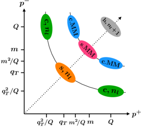
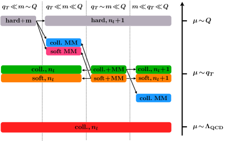
After discussing all hierarchies separately, we now show how the ingredients in each of the associated factorization theorems are related to each other. This will also make it obvious how the mass-dependent fixed-order corrections that are kept in one hierarchy but are dropped in another can be combined with the resummation of logarithms to obtain a systematic inclusion of the mass effects over the whole qTsubscript𝑞𝑇q_{T} spectrum. The relations between the modes and their contributions between the different regimes are summarized in fig. 4.
Refer to caption
Figure 4: Relevant modes for the qTsubscript𝑞𝑇q_{T} spectrum with qTQmuch-less-thansubscript𝑞𝑇𝑄q_{T}\ll Q for different hierarchies between the quark mass m𝑚m and the scales qTsubscript𝑞𝑇q_{T} and Q𝑄Q. The arrows indicate the relations between the modes and their associated contributions.

The hard functions appearing in the hierarchy qTmQmuch-less-thansubscript𝑞𝑇𝑚much-less-than𝑄q_{T}\ll m\ll Q in eq. (2.3) are related to the hard function for qTmQmuch-less-thansubscript𝑞𝑇𝑚similar-to𝑄q_{T}\ll m\sim Q in sec. 2.2 as follows555Here and in the following it is implied that at a specific fixed order the functions on both sides have to be expanded in the same renormalization scheme for αssubscript𝛼𝑠\alpha_{s}. Since Hij(nl+1)subscriptsuperscript𝐻subscript𝑛𝑙1𝑖𝑗H^{(n_{l}+1)}_{ij} is generically written with nl+1subscript𝑛𝑙1n_{l}+1 (massless) flavors, the (nl+1)subscript𝑛𝑙1(n_{l}+1)-flavor scheme is most convenient here and also to extract the 𝒪(m2/Q2)𝒪superscript𝑚2superscript𝑄2\mathcal{O}(m^{2}/Q^{2}) power corrections on the right-hand side of eq. (22) from its fixed-order expansion.

Hij(Q,m,μ)=Hij(nl+1)(Q,μ)Hc(m,μ,νωa)Hc(m,μ,νωb)Hs(m,μ,ν)[1+𝒪(m2Q2)].subscript𝐻𝑖𝑗𝑄𝑚𝜇subscriptsuperscript𝐻subscript𝑛𝑙1𝑖𝑗𝑄𝜇subscript𝐻𝑐𝑚𝜇𝜈subscript𝜔𝑎subscript𝐻𝑐𝑚𝜇𝜈subscript𝜔𝑏subscript𝐻𝑠𝑚𝜇𝜈delimited-[]1𝒪superscript𝑚2superscript𝑄2\displaystyle H_{ij}(Q,m,\mu)=H^{(n_{l}+1)}_{ij}(Q,\mu)\,H_{c}\Bigl{(}m,\mu,\frac{\nu}{\omega_{a}}\Bigr{)}H_{c}\Bigl{(}m,\mu,\frac{\nu}{\omega_{b}}\Bigr{)}H_{s}(m,\mu,\nu)\biggl{[}1+\mathcal{O}\Bigl{(}\frac{m^{2}}{Q^{2}}\Bigr{)}\biggr{]}\,. (22)

In the product of functions on the right-hand side, which appear in eq. (2.3), the logarithms ln(m/Q)𝑚𝑄\ln(m/Q) can be resummed to all orders. One can construct a smooth description of the cross section for qTmmuch-less-thansubscript𝑞𝑇𝑚q_{T}\ll m that resums these logarithms and also includes the associated mass-dependent 𝒪(m2/Q2)𝒪superscript𝑚2superscript𝑄2\mathcal{O}(m^{2}/Q^{2}) power corrections by simply adding the latter to the hard function H(nl+1)(Q,μ)superscript𝐻subscript𝑛𝑙1𝑄𝜇H^{(n_{l}+1)}(Q,\mu) at the scale μQsimilar-to𝜇𝑄\mu\sim Q.

The fixed-order contributions to the operator matrix elements appearing in the hierarchy qTmmuch-less-thansubscript𝑞𝑇𝑚q_{T}\ll m are encoded in the ones for qTmsimilar-tosubscript𝑞𝑇𝑚q_{T}\sim m. The mass-dependent beam function matching coefficients for qTmsimilar-tosubscript𝑞𝑇𝑚q_{T}\sim m are related to those for qTmmuch-less-thansubscript𝑞𝑇𝑚q_{T}\ll m and the collinear mass-mode function Hcsubscript𝐻𝑐H_{c} by

ik(pT,x,m,μ,νω)=Hc(m,μ,νω)ik(nl)(pT,x,μ,νω)[1+𝒪(pT2m2)].subscript𝑖𝑘subscript𝑝𝑇𝑥𝑚𝜇𝜈𝜔subscript𝐻𝑐𝑚𝜇𝜈𝜔superscriptsubscript𝑖𝑘subscript𝑛𝑙subscript𝑝𝑇𝑥𝜇𝜈𝜔delimited-[]1𝒪superscriptsubscript𝑝𝑇2superscript𝑚2\displaystyle\mathcal{I}_{ik}\Bigl{(}\vec{p}_{T},x,m,\mu,\frac{\nu}{\omega}\Bigr{)}=H_{c}\Bigl{(}m,\mu,\frac{\nu}{\omega}\Bigr{)}\,\mathcal{I}_{ik}^{(n_{l})}\Bigl{(}\vec{p}_{T},x,\mu,\frac{\nu}{\omega}\Bigr{)}\biggl{[}1+\mathcal{O}\Bigl{(}\frac{p_{T}^{2}}{m^{2}}\Bigr{)}\biggr{]}\,. (23)

Similarly, the mass-dependent soft function for qTmsimilar-tosubscript𝑞𝑇𝑚q_{T}\sim m is related to the one for qTmmuch-less-thansubscript𝑞𝑇𝑚q_{T}\ll m and the soft mass-mode function Hssubscript𝐻𝑠H_{s} by

S(pT,m,μ,ν)=Hs(m,μ,ν)S(nl)(pT,μ,ν)[1+𝒪(pT2m2)].𝑆subscript𝑝𝑇𝑚𝜇𝜈subscript𝐻𝑠𝑚𝜇𝜈superscript𝑆subscript𝑛𝑙subscript𝑝𝑇𝜇𝜈delimited-[]1𝒪superscriptsubscript𝑝𝑇2superscript𝑚2\displaystyle S(\vec{p}_{T},m,\mu,\nu)=H_{s}(m,\mu,\nu)\,S^{(n_{l})}(\vec{p}_{T},\mu,\nu)\biggl{[}1+\mathcal{O}\Bigl{(}\frac{p_{T}^{2}}{m^{2}}\Bigr{)}\biggr{]}\,. (24)

In the products on the right-hand sides, which appear in eq. (2.3), logarithms ln(qT/m)subscript𝑞𝑇𝑚\ln(q_{T}/m) are resummed to all orders in the limit qTmmuch-less-thansubscript𝑞𝑇𝑚q_{T}\ll m. One can include the associated 𝒪(qT2/m2)𝒪superscriptsubscript𝑞𝑇2superscript𝑚2\mathcal{O}(q_{T}^{2}/m^{2}) power corrections that are important for qTmsimilar-tosubscript𝑞𝑇𝑚q_{T}\sim m, by obtaining them from the fixed-order expansions of eqs. (23) and (24) and adding them to the (nl)subscript𝑛𝑙(n_{l})-flavor beam function coefficients and soft function at the scale μqTsimilar-to𝜇subscript𝑞𝑇\mu\sim q_{T}.

Finally, the fixed-order contributions for the operator matrix elements appearing in the hierarchy mqTmuch-less-than𝑚subscript𝑞𝑇m\ll q_{T} are also encoded in the corresponding ones for qTmsimilar-tosubscript𝑞𝑇𝑚q_{T}\sim m. Hence, the mass-dependent beam function matching coefficients are related to those for mqTmuch-less-than𝑚subscript𝑞𝑇m\ll q_{T} and the PDF matching functions by

ik(pT,m,x,μ,νω)=j=q,q¯,gij(nl+1)(pT,x,μ,νω)xjk(m,x,μ)[1+𝒪(m2pT2)].subscript𝑖𝑘subscript𝑝𝑇𝑚𝑥𝜇𝜈𝜔subscript𝑗𝑞¯𝑞𝑔subscripttensor-product𝑥superscriptsubscript𝑖𝑗subscript𝑛𝑙1subscript𝑝𝑇𝑥𝜇𝜈𝜔subscript𝑗𝑘𝑚𝑥𝜇delimited-[]1𝒪superscript𝑚2superscriptsubscript𝑝𝑇2\displaystyle\mathcal{I}_{ik}\Bigl{(}\vec{p}_{T},m,x,\mu,\frac{\nu}{\omega}\Bigr{)}=\sum_{j=q,\bar{q},g}\mathcal{I}_{ij}^{(n_{l}+1)}\Bigl{(}\vec{p}_{T},x,\mu,\frac{\nu}{\omega}\Bigr{)}\otimes_{x}\mathcal{M}_{jk}(m,x,\mu)\biggl{[}1+\mathcal{O}\Bigl{(}\frac{m^{2}}{p_{T}^{2}}\Bigr{)}\biggr{]}\,. (25)

Similarly, the mass-dependent and massless soft function are related by

S(pT,m,μ,ν)=S(nl+1)(pT,μ,ν)[1+𝒪(m2pT2)],𝑆subscript𝑝𝑇𝑚𝜇𝜈superscript𝑆subscript𝑛𝑙1subscript𝑝𝑇𝜇𝜈delimited-[]1𝒪superscript𝑚2superscriptsubscript𝑝𝑇2\displaystyle S(\vec{p}_{T},m,\mu,\nu)=S^{(n_{l}+1)}(\vec{p}_{T},\mu,\nu)\biggl{[}1+\mathcal{O}\Bigl{(}\frac{m^{2}}{p_{T}^{2}}\Bigr{)}\biggr{]}\,, (26)

since there are no relevant soft IR fluctuations below the mass scale. In the functions on the right-hand sides, which appear in eq. (2.5), logarithms ln(m/qT)𝑚subscript𝑞𝑇\ln(m/q_{T}) can be resummed to all orders in the limit mqTmuch-less-than𝑚subscript𝑞𝑇m\ll q_{T}. This can be combined with the associated 𝒪(m2/qT2)𝒪superscript𝑚2superscriptsubscript𝑞𝑇2\mathcal{O}(m^{2}/q_{T}^{2}) power corrections relevant for qTmsimilar-tosubscript𝑞𝑇𝑚q_{T}\sim m, by obtaining them from the fixed-order expansions of eqs. (25) and (26) and adding them to the (nl+1)subscript𝑛𝑙1(n_{l}+1)-flavor beam function matching coefficients and soft function at the scale μqTsimilar-to𝜇subscript𝑞𝑇\mu\sim q_{T}.

By including the various power corrections, one combines the factorization theorems in the different hierarchies and obtains a theoretical description that is valid across the whole qTsubscript𝑞𝑇q_{T} spectrum and includes the resummation of logarithms in all relevant limits. This can be considered a variable-flavor scheme for the resummed qTsubscript𝑞𝑇q_{T} spectrum. (In addition one should of course also include the usual qT/Qsubscript𝑞𝑇𝑄q_{T}/Q nonsingular corrections to reproduce the full fixed-order result for qTQsimilar-tosubscript𝑞𝑇𝑄q_{T}\sim Q.)

We stress that different specific ways of how to incorporate the various power corrections are formally equivalent as long as the correct fixed-order expansion and the correct resummation is reproduced in each limit. Any differences then amount to resummation effects at power-suppressed level and are thus beyond the formal (leading-power) resummation accuracy.

A particular scheme (“S-ACOT”) to merge the mqTmuch-less-than𝑚subscript𝑞𝑇m\ll q_{T} and qTmsimilar-tosubscript𝑞𝑇𝑚q_{T}\sim m regimes was discussed in ref. Nadolsky:2002jr for the primary massive quark corrections. In practice, for the numerical study of b𝑏b-quark mass effects at low qTmQmuch-less-thansubscript𝑞𝑇𝑚much-less-than𝑄q_{T}\ll m\ll Q the off-diagonal evolution factor Uf,bgsubscript𝑈𝑓𝑏𝑔U_{f,bg} and thus the effective b𝑏b-quark PDF at the scale qTsubscript𝑞𝑇q_{T} are still quite small, so that one may effectively count fb(μB)𝒪(αs)similar-tosubscript𝑓𝑏subscript𝜇𝐵𝒪subscript𝛼𝑠f_{b}(\mu_{B})\sim\mathcal{O}(\alpha_{s}). In particular, this counting facilitates the seamless combination with the nonsingular corrections for mqTsimilar-to𝑚subscript𝑞𝑇m\sim q_{T} encoded in the beam function matching coefficients in eq. (2.4). This was discussed in ref. Bonvini:2015pxa in the context of the inclusive bb¯H𝑏¯𝑏𝐻b\bar{b}H production cross section, and the analogous discussion applies here as well. In refs. Pietrulewicz:2014qza ; Hoang:2015iva , the power corrections were included implicitly in the construction of the variable-flavor number schemes for thrust in e+esuperscript𝑒superscript𝑒e^{+}e^{-} and DIS in the endpoint region by applying different renormalization schemes for the massive quark contributions to the EFT operators above and below the mass scale.

3 Factorization of mass effects for beam thrust

3.1 Factorization for massless quarks

For the measurement of beam thrust with 𝒯Qmuch-less-than𝒯𝑄{\mathcal{T}}\ll Q the relevant EFT modes are nasubscript𝑛𝑎n_{a}-collinear, nbsubscript𝑛𝑏n_{b}–collinear and usoft modes with the scaling

na-collinear:subscript𝑛𝑎-collinear:\displaystyle n_{a}\text{-collinear:} pnaμ(𝒯,Q,Q𝒯),similar-tosuperscriptsubscript𝑝subscript𝑛𝑎𝜇𝒯𝑄𝑄𝒯\displaystyle\quad p_{n_{a}}^{\mu}\sim({\mathcal{T}},Q,\sqrt{Q{\mathcal{T}}})\,,
nb-collinear:subscript𝑛𝑏-collinear:\displaystyle n_{b}\text{-collinear:} pnbμ(Q,𝒯,Q𝒯),similar-tosuperscriptsubscript𝑝subscript𝑛𝑏𝜇𝑄𝒯𝑄𝒯\displaystyle\quad p_{n_{b}}^{\mu}\sim(Q,{\mathcal{T}},\sqrt{Q{\mathcal{T}}})\,,
usoft: pusμ(𝒯,𝒯,𝒯).similar-tosuperscriptsubscript𝑝𝑢𝑠𝜇𝒯𝒯𝒯\displaystyle\quad p_{us}^{\mu}\sim({\mathcal{T}},{\mathcal{T}},{\mathcal{T}})\,. (27)

The usoft and collinear modes are now separated in invariant mass, pus2𝒯2pna2pnb2Q𝒯similar-tosuperscriptsubscript𝑝𝑢𝑠2superscript𝒯2much-less-thansuperscriptsubscript𝑝subscript𝑛𝑎2similar-tosuperscriptsubscript𝑝subscript𝑛𝑏2similar-to𝑄𝒯p_{us}^{2}\sim{\mathcal{T}}^{2}\ll p_{n_{a}}^{2}\sim p_{n_{b}}^{2}\sim Q{\mathcal{T}}, which is the characteristic feature of a SCETIsubscriptSCETI{\rm SCET}_{\rm I} theory. In this case, there are no rapidity logarithms and the renormalization and evolution is solely in invariant mass. The resulting factorization formula reads Stewart:2009yx

dσdQ2dYd𝒯d𝜎dsuperscript𝑄2d𝑌d𝒯\displaystyle\frac{\textrm{d}\sigma}{\textrm{d}Q^{2}\,\textrm{d}Y\,\textrm{d}{\mathcal{T}}} =i,j{q,q¯}Hij(nf)(Q,μ)dtadtbBi(nf)(ta,xa,μ)Bj(nf)(tb,xb,μ)absentsubscript𝑖𝑗𝑞¯𝑞subscriptsuperscript𝐻subscript𝑛𝑓𝑖𝑗𝑄𝜇dsubscript𝑡𝑎dsubscript𝑡𝑏subscriptsuperscript𝐵subscript𝑛𝑓𝑖subscript𝑡𝑎subscript𝑥𝑎𝜇subscriptsuperscript𝐵subscript𝑛𝑓𝑗subscript𝑡𝑏subscript𝑥𝑏𝜇\displaystyle=\sum_{i,j\in\{q,\bar{q}\}}H^{(n_{f})}_{ij}(Q,\mu)\int\textrm{d}t_{a}\,\textrm{d}t_{b}\,B^{(n_{f})}_{i}(t_{a},x_{a},\mu)\,B^{(n_{f})}_{j}(t_{b},x_{b},\mu)
×S(nf)(𝒯taωatbωb,μ)[1+𝒪(𝒯Q)].absentsuperscript𝑆subscript𝑛𝑓𝒯subscript𝑡𝑎subscript𝜔𝑎subscript𝑡𝑏subscript𝜔𝑏𝜇delimited-[]1𝒪𝒯𝑄\displaystyle\quad\times S^{(n_{f})}\Bigl{(}{\mathcal{T}}-\frac{t_{a}}{\omega_{a}}-\frac{t_{b}}{\omega_{b}},\mu\Bigr{)}\,\biggl{[}1+\mathcal{O}\Bigl{(}\frac{{\mathcal{T}}}{Q}\Bigr{)}\biggr{]}\,. (28)

This as well as the expressions including mass effects in the subsequent subsections are valid for the primary hard scattering, and do not account for spectator forward (multiparton) scattering effects, since the Glauber Lagrangian of ref. Rothstein:2016bsq has been neglected. (There are also corrections from perturbative Glauber effects starting at 𝒪(αs4)𝒪superscriptsubscript𝛼𝑠4{\cal O}(\alpha_{s}^{4}) Gaunt:2014ska ; Zeng:2015iba , which are well beyond the order we are interested in, but can be calculated and included using the Glauber operator framework of ref. Rothstein:2016bsq .) This is sufficient for our purposes of discussing the mass effects in a prototypical SCETIsubscriptSCETI{\rm SCET}_{\rm I} scenario. Our results are also directly relevant to include massive quark effects in the Geneva Monte-Carlo program Alioli:2012fc ; Alioli:2015toa , which employs 𝒯𝒯{\mathcal{T}} as the jet resolution variable for the primary interaction and where multiparton effects are included Alioli:2016wqt via the combination with Pythia8 and its MPI model Sjostrand:1987su ; Sjostrand:2004pf ; Sjostrand:2004ef .

The hard function Hijsubscript𝐻𝑖𝑗H_{ij} in eq. (3.1) is measurement independent and the same as in eq. (4). The beam and soft functions depend on the measurement and are different from those in eq. (4). The virtuality-dependent beam functions Bisubscript𝐵𝑖B_{i} can be factorized into perturbative matching coefficients iksubscript𝑖𝑘\mathcal{I}_{ik} at the scale μtQ𝒯similar-to𝜇𝑡similar-to𝑄𝒯\mu\sim t\sim\sqrt{Q{\mathcal{T}}} and the standard nonperturbative PDFs Stewart:2009yx ; Stewart:2010qs

Bi(nf)(t,x,μ)=kik(nf)(t,x,μ)xfk(nf)(x,μ)[1+𝒪(ΛQCD2t)].subscriptsuperscript𝐵subscript𝑛𝑓𝑖𝑡𝑥𝜇subscript𝑘subscripttensor-product𝑥subscriptsuperscriptsubscript𝑛𝑓𝑖𝑘𝑡𝑥𝜇subscriptsuperscript𝑓subscript𝑛𝑓𝑘𝑥𝜇delimited-[]1𝒪superscriptsubscriptΛQCD2𝑡\displaystyle B^{(n_{f})}_{i}(t,x,\mu)=\sum_{k}\mathcal{I}^{(n_{f})}_{ik}(t,x,\mu)\otimes_{x}f^{(n_{f})}_{k}(x,\mu)\biggl{[}1+\mathcal{O}\biggl{(}\frac{\Lambda_{\mathrm{QCD}}^{2}}{t}\biggr{)}\biggr{]}\,. (29)

The matching coefficients iksubscript𝑖𝑘\mathcal{I}_{ik} have been calculated to 𝒪(αs2)𝒪superscriptsubscript𝛼𝑠2\mathcal{O}(\alpha_{s}^{2}) Gaunt:2014xga ; Gaunt:2014cfa . The soft function at the scale μ𝒯similar-to𝜇𝒯\mu\sim{\mathcal{T}} is equivalent to the thrust soft function Kang:2015moa , which is known to 𝒪(αs2)𝒪superscriptsubscript𝛼𝑠2\mathcal{O}(\alpha_{s}^{2}) Kelley:2011ng ; Monni:2011gb . The noncusp anomalous dimensions required at N3LL are available from existing results Stewart:2010qs .

The resummation of logarithms ln(𝒯/Q)𝒯𝑄\ln({\mathcal{T}}/Q) is performed by evaluating all functions at their characteristic scales and evolving them to a common final scale μ𝜇\mu using the solutions of the RGEs

μddμBi(nf)(t,x,μ)𝜇dd𝜇subscriptsuperscript𝐵subscript𝑛𝑓𝑖𝑡𝑥𝜇\displaystyle\mu\frac{\textrm{d}}{\textrm{d}\mu}B^{(n_{f})}_{i}(t,x,\mu) =dtγB(nf)(tt,μ)Bi(nf)(t,x,μ),absentdsuperscript𝑡superscriptsubscript𝛾𝐵subscript𝑛𝑓𝑡superscript𝑡𝜇subscriptsuperscript𝐵subscript𝑛𝑓𝑖superscript𝑡𝑥𝜇\displaystyle=\int\textrm{d}t^{\prime}\,\gamma_{B}^{(n_{f})}(t-t^{\prime},\mu)\,B^{(n_{f})}_{i}(t^{\prime},x,\mu)\,,
μddμS(nf)(,μ)𝜇dd𝜇superscript𝑆subscript𝑛𝑓𝜇\displaystyle\mu\frac{\textrm{d}}{\textrm{d}\mu}S^{(n_{f})}(\ell,\mu) =dγS(nf)(,μ)S(nf)(,μ).absentdsuperscriptsuperscriptsubscript𝛾𝑆subscript𝑛𝑓superscript𝜇superscript𝑆subscript𝑛𝑓superscript𝜇\displaystyle=\int\textrm{d}\ell^{\prime}\,\gamma_{S}^{(n_{f})}(\ell-\ell^{\prime},\mu)\,S^{(n_{f})}(\ell^{\prime},\mu)\,. (30)

In contrast to eq. (4), there is no rapidity evolution in SCETIsubscriptSCETI{\rm SCET}_{\rm I} for massless quarks. Consistency of the RG evolution implies that

ωaγB(nf)(ωa,μ)+ωbγB(nf)(ωb,μ)+γS(nf)(,μ)=γH(nf)(Q,μ)δ().subscript𝜔𝑎superscriptsubscript𝛾𝐵subscript𝑛𝑓subscript𝜔𝑎𝜇subscript𝜔𝑏superscriptsubscript𝛾𝐵subscript𝑛𝑓subscript𝜔𝑏𝜇superscriptsubscript𝛾𝑆subscript𝑛𝑓𝜇superscriptsubscript𝛾𝐻subscript𝑛𝑓𝑄𝜇𝛿\displaystyle\omega_{a}\gamma_{B}^{(n_{f})}(\omega_{a}\ell,\mu)+\omega_{b}\gamma_{B}^{(n_{f})}(\omega_{b}\ell,\mu)+\gamma_{S}^{(n_{f})}(\ell,\mu)=\gamma_{H}^{(n_{f})}(Q,\mu)\,\delta(\ell)\,. (31)

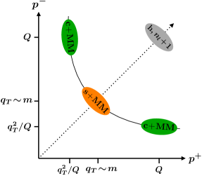
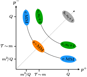
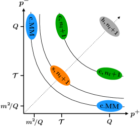
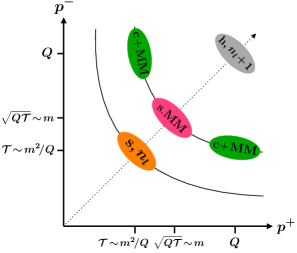
For beam thrust the number of possible scale hierarchies with a massive quark is larger due to the fact that the (massless) collinear and soft modes have different invariant mass scales. The discussion for the hierarchies with Q𝒯mmuch-less-than𝑄𝒯𝑚\sqrt{Q{\mathcal{T}}}\ll m where the massive quark cannot be produced via real emissions, is completely identical to qTmmuch-less-thansubscript𝑞𝑇𝑚q_{T}\ll m, since the quark mass effects in these cases are independent of the low-energy measurement. For mQsimilar-to𝑚𝑄m\sim Q, all mass effects are encoded by using the mass-dependent hard function from sec. 2.2 in eq. (3.1) together with nf=nlsubscript𝑛𝑓subscript𝑛𝑙n_{f}=n_{l} everywhere else. Similarly, the case Q𝒯mQmuch-less-than𝑄𝒯𝑚much-less-than𝑄\sqrt{Q{\mathcal{T}}}\ll m\ll Q is described by using eq. (3.1) with nf=nlsubscript𝑛𝑓subscript𝑛𝑙n_{f}=n_{l}, and replacing the hard function by the product of massless (nl+1)subscript𝑛𝑙1(n_{l}+1)-flavor hard function and the soft and collinear mass-mode functions Hssubscript𝐻𝑠H_{s} and Hcsubscript𝐻𝑐H_{c}, as for the case qTmQmuch-less-thansubscript𝑞𝑇𝑚much-less-than𝑄q_{T}\ll m\ll Q in sec. 2.3. We therefore proceed directly to the hierarchies mQ𝒯less-than-or-similar-to𝑚𝑄𝒯m\lesssim\sqrt{Q{\mathcal{T}}}, where the massive quark can be produced in collinear and/or soft real radiation. The four possible hierarchies and the relevant EFT modes in the p+psuperscript𝑝superscript𝑝p^{+}p^{-}-plane are illustrated in fig. 5, and are discussed in the following subsections.
Refer to caption
(a) 𝒯mQ𝒯much-less-than𝒯𝑚similar-to𝑄𝒯{{\mathcal{T}}\ll m\sim\sqrt{Q{\mathcal{T}}}}
Refer to caption
(b) 𝒯mQ𝒯much-less-than𝒯𝑚much-less-than𝑄𝒯{{\mathcal{T}}\ll m\ll\sqrt{Q{\mathcal{T}}}}
Refer to caption
(c) 𝒯mQ𝒯similar-to𝒯𝑚much-less-than𝑄𝒯{{\mathcal{T}}\sim m\ll\sqrt{Q{\mathcal{T}}}}
Refer to caption
(d) m𝒯Q𝒯much-less-than𝑚𝒯much-less-than𝑄𝒯{m\ll{\mathcal{T}}\ll\sqrt{Q{\mathcal{T}}}}
Figure 5: Effective theory modes for the beam thrust spectrum with massive quarks for m2/Q𝒯Qless-than-or-similar-tosuperscript𝑚2𝑄𝒯much-less-than𝑄m^{2}/Q\lesssim{\mathcal{T}}\ll Q and mΛQCDmuch-greater-than𝑚subscriptΛQCDm\gg\Lambda_{\rm QCD}.

3.2 Quark mass effects for Q𝒯mQsimilar-to𝑄𝒯𝑚much-less-than𝑄\sqrt{Q{\mathcal{T}}}\sim m\ll Q

For Q𝒯mQsimilar-to𝑄𝒯𝑚much-less-than𝑄\sqrt{Q{\mathcal{T}}}\sim m\ll Q massive quarks can be produced via collinear initial-state radiation, but not via soft real radiation. After the hard matching, carried out with nl+1subscript𝑛𝑙1n_{l}+1 massless quark flavors as discussed in sec. 2.3, the degrees of freedom in the EFT are collinear and soft modes with the scaling

na-collinear + MM:subscript𝑛𝑎-collinear + MM:\displaystyle n_{a}\text{-collinear + MM:} pnaμ(𝒯,Q,Q𝒯)(m2Q,Q,m),similar-tosuperscriptsubscript𝑝subscript𝑛𝑎𝜇𝒯𝑄𝑄𝒯similar-tosuperscript𝑚2𝑄𝑄𝑚\displaystyle\quad p_{n_{a}}^{\mu}\sim({\mathcal{T}},Q,\sqrt{Q{\mathcal{T}}})\sim\Bigl{(}\frac{m^{2}}{Q},Q,m\Bigr{)}\,,
nb-collinear + MM:subscript𝑛𝑏-collinear + MM:\displaystyle n_{b}\text{-collinear + MM:} pnbμ(Q,𝒯,Q𝒯)(Q,m2Q,m),similar-tosuperscriptsubscript𝑝subscript𝑛𝑏𝜇𝑄𝒯𝑄𝒯similar-to𝑄superscript𝑚2𝑄𝑚\displaystyle\quad p_{n_{b}}^{\mu}\sim(Q,{\mathcal{T}},\sqrt{Q{\mathcal{T}}})\sim\Bigl{(}Q,\frac{m^{2}}{Q},m\Bigr{)}\,,
soft MM: psμ(m,m,m),similar-tosuperscriptsubscript𝑝𝑠𝜇𝑚𝑚𝑚\displaystyle\quad p_{s}^{\mu}\sim(m,m,m)\,,
usoft: pusμ(𝒯,𝒯,𝒯),similar-tosuperscriptsubscript𝑝𝑢𝑠𝜇𝒯𝒯𝒯\displaystyle\quad p_{us}^{\mu}\sim({\mathcal{T}},{\mathcal{T}},{\mathcal{T}})\,, (32)

as illustrated in fig. 5(a). While the usual usoft modes live at a lower virtuality scale than the collinear modes, the soft mass-modes are separated from the collinear modes only in rapidity, leading to a mix of SCETIsubscriptSCETI{\rm SCET}_{\rm I} and SCETIIsubscriptSCETII{\rm SCET}_{\rm II} features. In particular, there will be mass-related rapidity divergences.

At the scale μQ𝒯msimilar-to𝜇𝑄𝒯similar-to𝑚\mu\sim\sqrt{Q{\mathcal{T}}}\sim m this theory with nl+1subscript𝑛𝑙1n_{l}+1 dynamical quark flavors is matched onto a theory with nlsubscript𝑛𝑙n_{l} flavors integrating out also fluctuations related to initial-state collinear radiation of massless particles. The matching in the collinear sectors leads to mass-dependent beam function coefficients iksubscript𝑖𝑘\mathcal{I}_{ik},

Bi(nl+1)(t,m,x,μ,νω)=k{q,q¯,g}ik(t,m,x,μ,νω)xfk(nl)(x,μ)[1+𝒪(ΛQCD2m2,ΛQCD2t)],superscriptsubscript𝐵𝑖subscript𝑛𝑙1𝑡𝑚𝑥𝜇𝜈𝜔subscript𝑘𝑞¯𝑞𝑔subscripttensor-product𝑥subscript𝑖𝑘𝑡𝑚𝑥𝜇𝜈𝜔subscriptsuperscript𝑓subscript𝑛𝑙𝑘𝑥𝜇delimited-[]1𝒪superscriptsubscriptΛQCD2superscript𝑚2superscriptsubscriptΛQCD2𝑡\displaystyle B_{i}^{(n_{l}+1)}\Bigl{(}t,m,x,\mu,\frac{\nu}{\omega}\Bigr{)}=\sum_{k\in\{q,\bar{q},g\}}\mathcal{I}_{ik}\Bigl{(}t,m,x,\mu,\frac{\nu}{\omega}\Bigr{)}\otimes_{x}f^{(n_{l})}_{k}(x,\mu)\biggl{[}1+\mathcal{O}\Bigl{(}\frac{\Lambda_{\mathrm{QCD}}^{2}}{m^{2}},\frac{\Lambda_{\mathrm{QCD}}^{2}}{t}\Bigr{)}\biggr{]}\,, (33)

analogous to eq. (14). The dependence on the rapidity scale ν𝜈\nu here arises due to virtual secondary massive quark corrections and is the same as for the collinear mass-mode function Hcsubscript𝐻𝑐H_{c} in eq. (2.3), i.e.,

νddνBi(nl+1)(t,m,x,μ,νω)=γν,Hc(m,μ)Bi(nl+1)(t,m,x,μ,νω).𝜈dd𝜈superscriptsubscript𝐵𝑖subscript𝑛𝑙1𝑡𝑚𝑥𝜇𝜈𝜔subscript𝛾𝜈subscript𝐻𝑐𝑚𝜇superscriptsubscript𝐵𝑖subscript𝑛𝑙1𝑡𝑚𝑥𝜇𝜈𝜔\displaystyle\nu\frac{\textrm{d}}{\textrm{d}\nu}B_{i}^{(n_{l}+1)}\Bigl{(}t,m,x,\mu,\frac{\nu}{\omega}\Bigr{)}=\gamma_{\nu,H_{c}}(m,\mu)\,B_{i}^{(n_{l}+1)}\Bigl{(}t,m,x,\mu,\frac{\nu}{\omega}\Bigr{)}\,. (34)

In the soft sector the soft mass modes are integrated out, leaving only the usoft modes. This gives exactly the soft mass-mode function Hssubscript𝐻𝑠H_{s} in eq. (2.3), which encodes the effects of virtual secondary massive quark radiation. As usual, also the strong coupling constant has to be matched from nl+1subscript𝑛𝑙1n_{l}+1 to nlsubscript𝑛𝑙n_{l} flavors. The remaining contributions at the lower scales, the soft function and the PDFs, are given in terms of nlsubscript𝑛𝑙n_{l} massless flavors and in the (nl)subscript𝑛𝑙(n_{l})-scheme for αssubscript𝛼𝑠\alpha_{s}. The resulting factorized cross section reads

dσdQ2dYd𝒯d𝜎dsuperscript𝑄2d𝑌d𝒯\displaystyle\frac{\textrm{d}\sigma}{\textrm{d}Q^{2}\,\textrm{d}Y\,\textrm{d}{\mathcal{T}}} =i,j{q,q¯,Q,Q¯}Hij(nl+1)(Q,μ)Hs(m,μ,ν)dtadtbabsentsubscript𝑖𝑗𝑞¯𝑞𝑄¯𝑄subscriptsuperscript𝐻subscript𝑛𝑙1𝑖𝑗𝑄𝜇subscript𝐻𝑠𝑚𝜇𝜈dsubscript𝑡𝑎dsubscript𝑡𝑏\displaystyle=\sum_{i,j\in\{q,\bar{q},Q,\bar{Q}\}}H^{(n_{l}+1)}_{ij}(Q,\mu)\,H_{s}(m,\mu,\nu)\int\!\textrm{d}t_{a}\,\textrm{d}t_{b}\,
×[k{q,q¯,g}ik(ta,m,xa,μ,νωa)xfk(nl)(xa,μ)]absentdelimited-[]subscript𝑘𝑞¯𝑞𝑔subscripttensor-product𝑥subscript𝑖𝑘subscript𝑡𝑎𝑚subscript𝑥𝑎𝜇𝜈subscript𝜔𝑎subscriptsuperscript𝑓subscript𝑛𝑙𝑘subscript𝑥𝑎𝜇\displaystyle\quad\times\biggl{[}\sum_{k\in\{q,\bar{q},g\}}\mathcal{I}_{ik}\Bigl{(}t_{a},m,x_{a},\mu,\frac{\nu}{\omega_{a}}\Bigr{)}\otimes_{x}f^{(n_{l})}_{k}(x_{a},\mu)\biggr{]}
×[k{q,q¯,g}jk(tb,m,xb,μ,νωa)xfk(nl)(xb,μ)]absentdelimited-[]subscript𝑘𝑞¯𝑞𝑔subscripttensor-product𝑥subscript𝑗𝑘subscript𝑡𝑏𝑚subscript𝑥𝑏𝜇𝜈subscript𝜔𝑎subscriptsuperscript𝑓subscript𝑛𝑙𝑘subscript𝑥𝑏𝜇\displaystyle\quad\times\biggl{[}\sum_{k\in\{q,\bar{q},g\}}\mathcal{I}_{jk}\Bigl{(}t_{b},m,x_{b},\mu,\frac{\nu}{\omega_{a}}\Bigr{)}\otimes_{x}f^{(n_{l})}_{k}(x_{b},\mu)\biggr{]}
×S(nl)(𝒯taωatbωb,μ)[1+𝒪(𝒯Q,m2Q2,𝒯2m2,ΛQCD𝒯)].absentsuperscript𝑆subscript𝑛𝑙𝒯subscript𝑡𝑎subscript𝜔𝑎subscript𝑡𝑏subscript𝜔𝑏𝜇delimited-[]1𝒪𝒯𝑄superscript𝑚2superscript𝑄2superscript𝒯2superscript𝑚2subscriptΛQCD𝒯\displaystyle\quad\times S^{(n_{l})}\Bigl{(}{\mathcal{T}}-\frac{t_{a}}{\omega_{a}}-\frac{t_{b}}{\omega_{b}},\mu\Bigr{)}\,\biggl{[}1+\mathcal{O}\Bigl{(}\frac{{\mathcal{T}}}{Q},\frac{m^{2}}{Q^{2}},\frac{{\mathcal{T}}^{2}}{m^{2}},\frac{\Lambda_{\mathrm{QCD}}}{{\mathcal{T}}}\Bigr{)}\biggr{]}\,. (35)

The resummation of logarithms in eq. (3.2) is obtained by evolving all functions from their natural scales, as illustrated in fig. 6(a). The mass-dependent ν𝜈\nu evolution, which resums the rapidity logarithms ln(Q/m)𝑄𝑚\ln(Q/m), is identical to the one for the hard functions Hcsubscript𝐻𝑐H_{c} and Hssubscript𝐻𝑠H_{s} in sec. 2.3. The μ𝜇\mu evolution can be conveniently carried out by evolving the hard, beam, and soft functions with nl+1subscript𝑛𝑙1n_{l}+1 active flavors above the mass scale and with nlsubscript𝑛𝑙n_{l} active flavors below the mass scale, which automatically takes into account the μ𝜇\mu dependence of HSsubscript𝐻𝑆H_{S}. To see this, the consistency of RG running for eq. (3.2) together with the consistency relation for nl+1subscript𝑛𝑙1n_{l}+1 massless quarks in eq. (31) implies

ωaγB,m(nl+1)(ωa,m,μ,νωa)+ωbγB,m(nl+1)(ωb,m,μ,νωb)+γS(nl)(,μ)+γHs,μ(m,μ,ν)δ()subscript𝜔𝑎superscriptsubscript𝛾𝐵𝑚subscript𝑛𝑙1subscript𝜔𝑎𝑚𝜇𝜈subscript𝜔𝑎subscript𝜔𝑏superscriptsubscript𝛾𝐵𝑚subscript𝑛𝑙1subscript𝜔𝑏𝑚𝜇𝜈subscript𝜔𝑏superscriptsubscript𝛾𝑆subscript𝑛𝑙𝜇subscript𝛾subscript𝐻𝑠𝜇𝑚𝜇𝜈𝛿\displaystyle\omega_{a}\gamma_{B,m}^{(n_{l}+1)}\Bigl{(}\omega_{a}\ell,m,\mu,\frac{\nu}{\omega_{a}}\Bigr{)}+\omega_{b}\gamma_{B,m}^{(n_{l}+1)}\Bigl{(}\omega_{b}\ell,m,\mu,\frac{\nu}{\omega_{b}}\Bigr{)}+\gamma_{S}^{(n_{l})}(\ell,\mu)+\gamma_{H_{s},\mu}(m,\mu,\nu)\,\delta(\ell)
=ωaγB(nl+1)(ωa,μ)+ωbγB(nl+1)(ωb,μ)+γS(nl+1)(,μ),absentsubscript𝜔𝑎superscriptsubscript𝛾𝐵subscript𝑛𝑙1subscript𝜔𝑎𝜇subscript𝜔𝑏superscriptsubscript𝛾𝐵subscript𝑛𝑙1subscript𝜔𝑏𝜇superscriptsubscript𝛾𝑆subscript𝑛𝑙1𝜇\displaystyle\qquad=\omega_{a}\gamma_{B}^{(n_{l}+1)}(\omega_{a}\ell,\mu)+\omega_{b}\gamma_{B}^{(n_{l}+1)}(\omega_{b}\ell,\mu)+\gamma_{S}^{(n_{l}+1)}(\ell,\mu)\,, (36)

where γS(nl)superscriptsubscript𝛾𝑆subscript𝑛𝑙\gamma_{S}^{(n_{l})}, γS(nl+1)superscriptsubscript𝛾𝑆subscript𝑛𝑙1\gamma_{S}^{(n_{l}+1)}, γB(nl+1)superscriptsubscript𝛾𝐵subscript𝑛𝑙1\gamma_{B}^{(n_{l}+1)} are the anomalous dimensions for the soft and beam functions with nlsubscript𝑛𝑙n_{l} and nl+1subscript𝑛𝑙1n_{l}+1 massless flavors as defined in eq. (3.1), and γB,m(nl+1)(t,m,μ,ν/ω)superscriptsubscript𝛾𝐵𝑚subscript𝑛𝑙1𝑡𝑚𝜇𝜈𝜔\gamma_{B,m}^{(n_{l}+1)}(t,m,\mu,\nu/\omega) is the anomalous dimension of the mass-dependent beam function,

μddμBi(nl+1)(t,m,x,μ,νω)=dtγB,m(nl+1)(tt,m,μ,νω)Bi(nl+1)(t,m,x,μ,νω).𝜇dd𝜇superscriptsubscript𝐵𝑖subscript𝑛𝑙1𝑡𝑚𝑥𝜇𝜈𝜔dsuperscript𝑡superscriptsubscript𝛾𝐵𝑚subscript𝑛𝑙1𝑡superscript𝑡𝑚𝜇𝜈𝜔superscriptsubscript𝐵𝑖subscript𝑛𝑙1superscript𝑡𝑚𝑥𝜇𝜈𝜔\displaystyle\mu\frac{\textrm{d}}{\textrm{d}\mu}B_{i}^{(n_{l}+1)}\Bigl{(}t,m,x,\mu,\frac{\nu}{\omega}\Bigr{)}=\int\textrm{d}t^{\prime}\,\gamma_{B,m}^{(n_{l}+1)}\Bigl{(}t-t^{\prime},m,\mu,\frac{\nu}{\omega}\Bigr{)}\,B_{i}^{(n_{l}+1)}\Bigl{(}t^{\prime},m,x,\mu,\frac{\nu}{\omega}\Bigr{)}\,. (37)

The consistency relation in eq. (3.2) can be confirmed explicitly at two loops with the expressions in eqs. (A.2.2), (A.3.2), (4.1.2), and (73). Note that this relation does not imply that γB,m(nl+1)(t,m,μ,ν/ω)superscriptsubscript𝛾𝐵𝑚subscript𝑛𝑙1𝑡𝑚𝜇𝜈𝜔\gamma_{B,m}^{(n_{l}+1)}(t,m,\mu,\nu/\omega) and γB(nl+1)(t,μ)superscriptsubscript𝛾𝐵subscript𝑛𝑙1𝑡𝜇\gamma_{B}^{(n_{l}+1)}(t,\mu) are the same, which is indeed not the case for the massive quark corrections as we will see explicitly in sec. 4.2. The reason is that the presence of the quark mass leads to a SCETIIsubscriptSCETII{\rm SCET}_{\rm II}-type theory, in which the required rapidity regularization redistributes the μ𝜇\mu anomalous dimension between soft and collinear corrections with individually regularization scheme dependent pieces. Only their sum, as given on the left-hand side of eq. (3.2), is independent of the regularization scheme and yields the combined running for beam and soft functions with nl+1subscript𝑛𝑙1n_{l}+1 massless flavors above μmmsimilar-tosubscript𝜇𝑚𝑚\mu_{m}\sim m, as on the right-hand side of eq. (3.2).
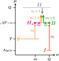
Refer to caption
(a) 𝒯mQ𝒯much-less-than𝒯𝑚similar-to𝑄𝒯{{\mathcal{T}}\ll m\sim\sqrt{Q{\mathcal{T}}}}
Refer to caption
(b) 𝒯mQ𝒯much-less-than𝒯𝑚much-less-than𝑄𝒯{{\mathcal{T}}\ll m\ll\sqrt{Q{\mathcal{T}}}}
Refer to caption
(c) 𝒯mQ𝒯similar-to𝒯𝑚much-less-than𝑄𝒯{{\mathcal{T}}\sim m\ll\sqrt{Q{\mathcal{T}}}}
Figure 6: Illustration of the renormalization group evolution for beam thrust of the hard, beam, soft, and parton distribution function in invariant mass and rapidity. The anomalous dimensions for each evolution step involve the displayed number of active quark flavors. The label m𝑚m indicates that the corresponding evolution is mass dependent.

3.3 Quark mass effects for 𝒯mQ𝒯much-less-than𝒯𝑚much-less-than𝑄𝒯{\mathcal{T}}\ll m\ll\sqrt{Q{\mathcal{T}}}

When the beam scale becomes larger than the mass scale, but the soft scale is still larger than the mass, which happens for m2/Q𝒯mmuch-less-thansuperscript𝑚2𝑄𝒯much-less-than𝑚m^{2}/Q\ll{\mathcal{T}}\ll m, the beam function matching coefficients iksubscript𝑖𝑘\mathcal{I}_{ik} encode only fluctuations related to initial-state collinear radiation with nl+1subscript𝑛𝑙1n_{l}+1 massless quarks. The EFT below Q𝒯𝑄𝒯\sqrt{Q{\mathcal{T}}} contains the usual collinear and soft mass modes scaling as pm,naμ(m2/Q,Q,m)similar-tosuperscriptsubscript𝑝𝑚subscript𝑛𝑎𝜇superscript𝑚2𝑄𝑄𝑚p_{m,n_{a}}^{\mu}\sim(m^{2}/Q,Q,m), pm,nbμ(Q,m2/Q,m)similar-tosuperscriptsubscript𝑝𝑚subscript𝑛𝑏𝜇𝑄superscript𝑚2𝑄𝑚p_{m,n_{b}}^{\mu}\sim(Q,m^{2}/Q,m), and pm,sμ(m,m,m)similar-tosuperscriptsubscript𝑝𝑚𝑠𝜇𝑚𝑚𝑚p_{m,s}^{\mu}\sim(m,m,m), which do not contribute to the beam thrust measurement. However, besides these there are also additional modes with fluctuations around the mass scale which can have a dynamic impact on the 𝒯𝒯{\mathcal{T}} spectrum in this hierarchy, as illustrated in fig. 5(b). Their scaling is precisely determined by this condition and the on-shell constraint, yielding the scaling

na-csoft MM:subscript𝑛𝑎-csoft MM:\displaystyle n_{a}\text{-csoft MM:} pcs,naμ(𝒯,m2𝒯,m),similar-tosuperscriptsubscript𝑝𝑐𝑠subscript𝑛𝑎𝜇𝒯superscript𝑚2𝒯𝑚\displaystyle\quad p_{cs,n_{a}}^{\mu}\sim\Bigl{(}{\mathcal{T}},\frac{m^{2}}{{\mathcal{T}}},m\Bigr{)}\,,
nb-csoft MM:subscript𝑛𝑏-csoft MM:\displaystyle n_{b}\text{-csoft MM:} pcs,nbμ(m2𝒯,𝒯,m).similar-tosuperscriptsubscript𝑝𝑐𝑠subscript𝑛𝑏𝜇superscript𝑚2𝒯𝒯𝑚\displaystyle\quad p_{cs,n_{b}}^{\mu}\sim\Bigl{(}\frac{m^{2}}{{\mathcal{T}}},{\mathcal{T}},m\Bigr{)}\,. (38)

We refer to these intermediate modes as collinear-soft (csoft), since they are simultaneously boosted (by a factor m/𝒯𝑚𝒯m/{\mathcal{T}}) but are softer than the standard collinear modes, thus coupling to the latter via Wilson lines and leading to a SCET+subscriptSCET{\rm SCET}_{+} theory Bauer:2011uc . This type of intermediate SCET+subscriptSCET{\rm SCET}_{+} modes have appeared in various contexts Bauer:2011uc ; Procura:2014cba ; Larkoski:2015zka ; Pietrulewicz:2016nwo . The setup here is similar to the case of double-differential distributions with a simultaneous qTsubscript𝑞𝑇q_{T} and beam thrust measurement discussed in ref. Procura:2014cba . Also there, several hierarchies are possible ranging from a SCETIIsubscriptSCETII{\rm SCET}_{\rm II} regime for qT𝒯similar-tosubscript𝑞𝑇𝒯q_{T}\sim{\mathcal{T}} to a SCETIsubscriptSCETI{\rm SCET}_{\rm I} regime for qTQ𝒯similar-tosubscript𝑞𝑇𝑄𝒯q_{T}\sim\sqrt{Q{\mathcal{T}}} with a SCET+subscriptSCET{\rm SCET}_{+} regime in between. The csoft modes in their SCET+subscriptSCET{\rm SCET}_{+} regime are separated from the collinear modes only in rapidity. In our case here, the csoft mass modes are separated in invariant mass from the standard SCETIsubscriptSCETI{\rm SCET}_{\rm I} soft and collinear modes and in rapidity from their SCETIIsubscriptSCETII{\rm SCET}_{\rm II}-type soft mass-mode cousins.

The matching in the collinear sector can be performed in two steps as in eqs. (18) and (19). After integrating out all of the mass modes, the PDF and the soft function are still given in a (nl)subscript𝑛𝑙(n_{l})-flavor theory. Thus the factorization formula reads

dσdQ2dYd𝒯d𝜎dsuperscript𝑄2d𝑌d𝒯\displaystyle\frac{\textrm{d}\sigma}{\textrm{d}Q^{2}\,\textrm{d}Y\,\textrm{d}{\mathcal{T}}} =i,j{q,q¯,Q,Q¯}Hij(nl+1)(Q,μ)Hs(m,μ,ν)dkadkb𝒮c(ka,m,μ,ν)𝒮c(kb,m,μ,ν)absentsubscript𝑖𝑗𝑞¯𝑞𝑄¯𝑄subscriptsuperscript𝐻subscript𝑛𝑙1𝑖𝑗𝑄𝜇subscript𝐻𝑠𝑚𝜇𝜈dsubscript𝑘𝑎dsubscript𝑘𝑏subscript𝒮𝑐subscript𝑘𝑎𝑚𝜇𝜈subscript𝒮𝑐subscript𝑘𝑏𝑚𝜇𝜈\displaystyle=\sum_{i,j\in\{q,\bar{q},Q,\bar{Q}\}}H^{(n_{l}+1)}_{ij}(Q,\mu)\,H_{s}(m,\mu,\nu)\int\!\textrm{d}k_{a}\,\textrm{d}k_{b}\,\mathcal{S}_{c}(k_{a},m,\mu,\nu)\,\mathcal{S}_{c}(k_{b},m,\mu,\nu)
×dta[k{q,q¯,Q,Q¯,g}l{q,q¯,g}ik(nl+1)(ta,xa,μ)xkl(xa,m,μ)xfk(nl)(xa,μ)]\displaystyle\quad\times\int\!\textrm{d}t_{a}\,\biggl{[}\sum_{k\in\{q,\bar{q},Q,\bar{Q},g\}}\sum_{l\in\{q,\bar{q},g\}}\mathcal{I}^{(n_{l}+1)}_{ik}(t_{a},x_{a},\mu)\otimes_{x}\mathcal{M}_{kl}(x_{a},m,\mu)\otimes_{x}f^{(n_{l})}_{k}(x_{a},\mu)\biggr{]}
×dtb[k{q,q¯,Q,Q¯,g}l{q,q¯,g}jk(nl+1)(tb,xb,μ)xkl(xb,m,μ)xfn(nl)(xb,μ)]\displaystyle\quad\times\int\!\textrm{d}t_{b}\,\biggl{[}\sum_{k\in\{q,\bar{q},Q,\bar{Q},g\}}\sum_{l\in\{q,\bar{q},g\}}\mathcal{I}^{(n_{l}+1)}_{jk}(t_{b},x_{b},\mu)\otimes_{x}\mathcal{M}_{kl}(x_{b},m,\mu)\otimes_{x}f^{(n_{l})}_{n}(x_{b},\mu)\biggr{]}
×S(nl)(𝒯taωatbωbkakb,μ)[1+𝒪(𝒯Q,m2Q𝒯,𝒯2m2,ΛQCD𝒯)].absentsuperscript𝑆subscript𝑛𝑙𝒯subscript𝑡𝑎subscript𝜔𝑎subscript𝑡𝑏subscript𝜔𝑏subscript𝑘𝑎subscript𝑘𝑏𝜇delimited-[]1𝒪𝒯𝑄superscript𝑚2𝑄𝒯superscript𝒯2superscript𝑚2subscriptΛQCD𝒯\displaystyle\quad\times S^{(n_{l})}\Bigl{(}{\mathcal{T}}-\frac{t_{a}}{\omega_{a}}-\frac{t_{b}}{\omega_{b}}-k_{a}-k_{b},\mu\Bigr{)}\Bigl{[}1+\mathcal{O}\Bigl{(}\frac{{\mathcal{T}}}{Q},\frac{m^{2}}{Q{\mathcal{T}}},\frac{{\mathcal{T}}^{2}}{m^{2}},\frac{\Lambda_{\mathrm{QCD}}}{{\mathcal{T}}}\Bigr{)}\Bigr{]}\,. (39)

The functions 𝒮csubscript𝒮𝑐\mathcal{S}_{c} here are the csoft matching functions encoding the interactions of the collinear-soft radiation at the invariant mass scale μmsimilar-to𝜇𝑚\mu\sim m and the rapidity scale νm2/𝒯similar-to𝜈superscript𝑚2𝒯\nu\sim m^{2}/{\mathcal{T}}. The ijsubscript𝑖𝑗\mathcal{M}_{ij} correspond to the well-known PDF matching correction incorporating the effect of the collinear mass modes, as in eq. (2.5). The virtual soft massive quark corrections are still described by the function Hssubscript𝐻𝑠H_{s} at the rapidity scale νmsimilar-to𝜈𝑚\nu\sim m as in eq. (3.2).

The RG evolution for eq. (3.3) is illustrated in fig. 6(b). The csoft function satisfies the same rapidity RGE as the collinear mass-mode function Hcsubscript𝐻𝑐H_{c} in eq. (2.3) and the massive beam functions in eq. (34), i.e.,

νddν𝒮c(k,m,μ,ν)=γν,Hc(m,μ)𝒮c(k,m,μ,ν).𝜈dd𝜈subscript𝒮𝑐𝑘𝑚𝜇𝜈subscript𝛾𝜈subscript𝐻𝑐𝑚𝜇subscript𝒮𝑐𝑘𝑚𝜇𝜈\displaystyle\nu\frac{\textrm{d}}{\textrm{d}\nu}\mathcal{S}_{c}(k,m,\mu,\nu)=\gamma_{\nu,H_{c}}(m,\mu)\,\mathcal{S}_{c}(k,m,\mu,\nu)\,. (40)

The only difference with respect to the rapidity evolution in eq. (3.2) is that it now happens between Hssubscript𝐻𝑠H_{s} and 𝒮csubscript𝒮𝑐\mathcal{S}_{c} with ν𝒮cm2/𝒯similar-tosubscript𝜈subscript𝒮𝑐superscript𝑚2𝒯\nu_{\mathcal{S}_{c}}\sim m^{2}/{\mathcal{T}} rather than between Hssubscript𝐻𝑠H_{s} and the beam functions with νBQsimilar-tosubscript𝜈𝐵𝑄\nu_{B}\sim Q, such that now the (smaller) rapidity logarithms ln(m/𝒯)𝑚𝒯\ln(m/{\mathcal{T}}) are resummed. The μ𝜇\mu evolution can be performed with nl+1subscript𝑛𝑙1n_{l}+1 flavors for the hard function Hijsubscript𝐻𝑖𝑗H_{ij}, the beam and soft function above the mass scale and with nlsubscript𝑛𝑙n_{l} flavors below. This automatically accounts for the μ𝜇\mu dependence of 𝒮csubscript𝒮𝑐\mathcal{S}_{c} and Hssubscript𝐻𝑠H_{s} above μmmsimilar-tosubscript𝜇𝑚𝑚\mu_{m}\sim m, which precisely gives the difference between the evolution of the soft function with nl+1subscript𝑛𝑙1n_{l}+1 and nlsubscript𝑛𝑙n_{l} flavors, as implied by the consistency of RG running for eq. (3.3) and the relation in eq. (31) with nl+1subscript𝑛𝑙1n_{l}+1 massless quarks,

γS(nl)(,μ)+2γ𝒮c(,m,μ,ν)+δ()γHs(m,μ,ν)=γS(nl+1)(,μ),superscriptsubscript𝛾𝑆subscript𝑛𝑙𝜇2subscript𝛾subscript𝒮𝑐𝑚𝜇𝜈𝛿subscript𝛾subscript𝐻𝑠𝑚𝜇𝜈superscriptsubscript𝛾𝑆subscript𝑛𝑙1𝜇\displaystyle\gamma_{S}^{(n_{l})}(\ell,\mu)+2\gamma_{\mathcal{S}_{c}}(\ell,m,\mu,\nu)+\delta(\ell)\,\gamma_{H_{s}}(m,\mu,\nu)=\gamma_{S}^{(n_{l}+1)}(\ell,\mu)\,, (41)

where

μddμ𝒮c(k,m,μ,ν)=dkγ𝒮c(kk,m,μ,ν)𝒮c(k,m,μ,ν).𝜇dd𝜇subscript𝒮𝑐𝑘𝑚𝜇𝜈dsuperscript𝑘subscript𝛾subscript𝒮𝑐𝑘superscript𝑘𝑚𝜇𝜈subscript𝒮𝑐𝑘𝑚𝜇𝜈\displaystyle\mu\frac{\textrm{d}}{\textrm{d}\mu}\mathcal{S}_{c}(k,m,\mu,\nu)=\int\textrm{d}k^{\prime}\,\gamma_{\mathcal{S}_{c}}(k-k^{\prime},m,\mu,\nu)\,\mathcal{S}_{c}(k,m,\mu,\nu)\,. (42)

At two loops, the consistency relation eq. (41) can be explicitly confirmed with the expressions in eqs. (A.3.2), (80), and (4.1.2).

3.4 Quark mass effects for 𝒯msimilar-to𝒯𝑚{\mathcal{T}}\sim m and m𝒯much-less-than𝑚𝒯m\ll{\mathcal{T}}

For 𝒯msimilar-to𝒯𝑚{\mathcal{T}}\sim m the csoft and soft mass modes in the previous section merge with the usual usoft modes,

usoft: psμ(𝒯,𝒯,𝒯)(𝒯,m2𝒯,m)(m,m,m).similar-tosuperscriptsubscript𝑝𝑠𝜇𝒯𝒯𝒯similar-to𝒯superscript𝑚2𝒯𝑚similar-to𝑚𝑚𝑚\displaystyle\quad p_{s}^{\mu}\sim({\mathcal{T}},{\mathcal{T}},{\mathcal{T}})\sim\Bigl{(}{\mathcal{T}},\frac{m^{2}}{{\mathcal{T}}},m\Bigr{)}\sim(m,m,m)\,. (43)

In this hierarchy massive quarks can be also produced in soft real radiation leading to a soft function at the scale μ𝒯similar-to𝜇𝒯\mu\sim{\mathcal{T}} that depends on the quark mass. In addition, there are the usual collinear modes as well as the collinear mass modes, as illustrated in fig. 5(c). Since we still have mQ𝒯much-less-than𝑚𝑄𝒯m\ll\sqrt{Q{\mathcal{T}}}, the matching in the collinear sectors is the same as in the previous subsection. The factorization formula reads

dσdQ2dYd𝒯d𝜎dsuperscript𝑄2d𝑌d𝒯\displaystyle\frac{\textrm{d}\sigma}{\textrm{d}Q^{2}\,\textrm{d}Y\,\textrm{d}{\mathcal{T}}} =i,j{q,q¯,Q,Q¯}Hij(nl+1)(Q,μ)dtadtbabsentsubscript𝑖𝑗𝑞¯𝑞𝑄¯𝑄subscriptsuperscript𝐻subscript𝑛𝑙1𝑖𝑗𝑄𝜇dsubscript𝑡𝑎dsubscript𝑡𝑏\displaystyle=\sum_{i,j\in\{q,\bar{q},Q,\bar{Q}\}}H^{(n_{l}+1)}_{ij}(Q,\mu)\int\!\textrm{d}t_{a}\,\textrm{d}t_{b}
×[k{q,q¯,Q,Q¯,g}l{q,q¯,g}ik(nl+1)(ta,xa,μ)xkl(xa,m,μ)xfk(nl)(xa,μ)]absentdelimited-[]subscript𝑘𝑞¯𝑞𝑄¯𝑄𝑔subscript𝑙𝑞¯𝑞𝑔subscripttensor-product𝑥subscripttensor-product𝑥subscriptsuperscriptsubscript𝑛𝑙1𝑖𝑘subscript𝑡𝑎subscript𝑥𝑎𝜇subscript𝑘𝑙subscript𝑥𝑎𝑚𝜇subscriptsuperscript𝑓subscript𝑛𝑙𝑘subscript𝑥𝑎𝜇\displaystyle\quad\times\biggl{[}\sum_{k\in\{q,\bar{q},Q,\bar{Q},g\}}\sum_{l\in\{q,\bar{q},g\}}\mathcal{I}^{(n_{l}+1)}_{ik}(t_{a},x_{a},\mu)\otimes_{x}\mathcal{M}_{kl}(x_{a},m,\mu)\otimes_{x}f^{(n_{l})}_{k}(x_{a},\mu)\biggr{]}
×[k{q,q¯,Q,Q¯,g}l{q,q¯,g}jk(nl+1)(tb,xb,μ)xkl(xb,m,μ)xfk(nl)(xb,μ)]absentdelimited-[]subscript𝑘𝑞¯𝑞𝑄¯𝑄𝑔subscript𝑙𝑞¯𝑞𝑔subscripttensor-product𝑥subscripttensor-product𝑥subscriptsuperscriptsubscript𝑛𝑙1𝑗𝑘subscript𝑡𝑏subscript𝑥𝑏𝜇subscript𝑘𝑙subscript𝑥𝑏𝑚𝜇subscriptsuperscript𝑓subscript𝑛𝑙𝑘subscript𝑥𝑏𝜇\displaystyle\quad\times\biggl{[}\sum_{k\in\{q,\bar{q},Q,\bar{Q},g\}}\sum_{l\in\{q,\bar{q},g\}}\mathcal{I}^{(n_{l}+1)}_{jk}(t_{b},x_{b},\mu)\otimes_{x}\mathcal{M}_{kl}(x_{b},m,\mu)\otimes_{x}f^{(n_{l})}_{k}(x_{b},\mu)\biggr{]}
×S(𝒯taωatbωb,m,μ)[1+𝒪(𝒯Q,m2Q𝒯,ΛQCD𝒯,ΛQCD2m2)].absent𝑆𝒯subscript𝑡𝑎subscript𝜔𝑎subscript𝑡𝑏subscript𝜔𝑏𝑚𝜇delimited-[]1𝒪𝒯𝑄superscript𝑚2𝑄𝒯subscriptΛQCD𝒯superscriptsubscriptΛQCD2superscript𝑚2\displaystyle\quad\times S\Bigl{(}{\mathcal{T}}-\frac{t_{a}}{\omega_{a}}-\frac{t_{b}}{\omega_{b}},m,\mu\Bigr{)}\biggl{[}1+\mathcal{O}\Bigl{(}\frac{{\mathcal{T}}}{Q},\frac{m^{2}}{Q{\mathcal{T}}},\frac{\Lambda_{\mathrm{QCD}}}{{\mathcal{T}}},\frac{\Lambda_{\mathrm{QCD}}^{2}}{m^{2}}\Bigr{)}\biggr{]}\,. (44)

Now all rapidity divergences cancel within the soft function and do not leave behind any potentially large rapidity logarithms. The RG evolution for this case is illustrated in fig. 6(c).

Finally, for m𝒯much-less-than𝑚𝒯m\ll{\mathcal{T}} the mass dependence in the IR insensitive soft function vanishes, if expressed in terms of the (nl+1)subscript𝑛𝑙1(n_{l}+1)-flavor scheme for αssubscript𝛼𝑠\alpha_{s}. Otherwise, eq. (3.4) remains unchanged, such that now the only dependence on the mass scale arises in the PDF matching corrections ijsubscript𝑖𝑗\mathcal{M}_{ij}. The hard, beam, and soft functions can now be always evolved with nl+1subscript𝑛𝑙1n_{l}+1 massless flavors and only the evolution of the PDF changes, when crossing the flavor threshold.

3.5 Relations between hierarchies
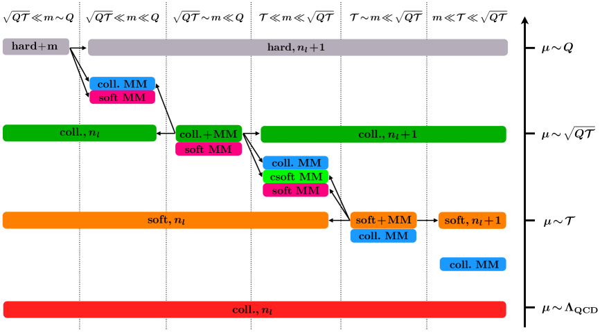
Refer to caption
Figure 7: Relevant modes for the beam thrust spectrum with 𝒯Qmuch-less-than𝒯𝑄{\mathcal{T}}\ll Q for different hierarchies between the quark mass m𝑚m and the scales 𝒯𝒯{\mathcal{T}}, Q𝒯𝑄𝒯\sqrt{Q{\mathcal{T}}} and Q𝑄Q. The arrows indicate the relations between the modes and their associated contributions.

We now discuss how the ingredients appearing in the different factorization formulae are related to each other. The relations between the modes and their contributions are illustrated in fig. 7 for the different possible hierarchies. As in sec. 2.6, these relations show how one can combine the resummation of logarithms relevant in one regime with the power-suppressed fixed-order content that becomes important in the neighboring regimes, enabling a systematic inclusion of mass corrections across the entire 𝒯𝒯{\mathcal{T}} spectrum.

Similar to eq. (23), the mass-dependent beam function coefficients appearing for Q𝒯msimilar-to𝑄𝒯𝑚\sqrt{Q{\mathcal{T}}}\sim m (incorporating massive quark fluctuation as discussed in sec. 3.2) are related to those for Q𝒯mmuch-less-than𝑄𝒯𝑚\sqrt{Q{\mathcal{T}}}\ll m with nlsubscript𝑛𝑙n_{l} massless quarks and the collinear mass-mode function Hcsubscript𝐻𝑐H_{c} by

ik(t,m,x,μ,νω)=Hc(m,μ,νω)ik(nl)(t,x,μ)[1+𝒪(tm2)].subscript𝑖𝑘𝑡𝑚𝑥𝜇𝜈𝜔subscript𝐻𝑐𝑚𝜇𝜈𝜔superscriptsubscript𝑖𝑘subscript𝑛𝑙𝑡𝑥𝜇delimited-[]1𝒪𝑡superscript𝑚2\displaystyle\mathcal{I}_{ik}\Bigl{(}t,m,x,\mu,\frac{\nu}{\omega}\Bigr{)}=H_{c}\Bigl{(}m,\mu,\frac{\nu}{\omega}\Bigr{)}\,\mathcal{I}_{ik}^{(n_{l})}(t,x,\mu)\Bigl{[}1+\mathcal{O}\Bigl{(}\frac{t}{m^{2}}\Bigr{)}\Bigr{]}\,. (45)

At the same time, the mass-dependent beam function also encodes information about the fixed-order content for 𝒯mQ𝒯much-less-than𝒯𝑚much-less-than𝑄𝒯{\mathcal{T}}\ll m\ll\sqrt{Q{\mathcal{T}}}. Comparing eqs. (3.2) and (3.3), they are related to those with nl+1subscript𝑛𝑙1n_{l}+1 massless flavors, the PDF matching functions, and the csoft function 𝒮csubscript𝒮𝑐\mathcal{S}_{c} by

ik(t,m,x,μ,νω)subscript𝑖𝑘𝑡𝑚𝑥𝜇𝜈𝜔\displaystyle\mathcal{I}_{ik}\Bigl{(}t,m,x,\mu,\frac{\nu}{\omega}\Bigr{)} =j={q,q¯,Q,Q¯,g}dij(nl+1)(tQ,x,μ)xjk(x,m,μ)𝒮c(,m,μ,ν)absentsubscript𝑗𝑞¯𝑞𝑄¯𝑄𝑔subscripttensor-product𝑥dsuperscriptsubscript𝑖𝑗subscript𝑛𝑙1𝑡𝑄𝑥𝜇subscript𝑗𝑘𝑥𝑚𝜇subscript𝒮𝑐𝑚𝜇𝜈\displaystyle=\!\!\sum_{j=\{q,\bar{q},Q,\bar{Q},g\}}\int\!\textrm{d}\ell\,\mathcal{I}_{ij}^{(n_{l}+1)}(t-Q\ell,x,\mu)\otimes_{x}\mathcal{M}_{jk}(x,m,\mu)\,\mathcal{S}_{c}(\ell,m,\mu,\nu)
×[1+𝒪(m2Q𝒯)].absentdelimited-[]1𝒪superscript𝑚2𝑄𝒯\displaystyle\quad\times\biggl{[}1+\mathcal{O}\Bigl{(}\frac{m^{2}}{Q{\mathcal{T}}}\Bigr{)}\biggr{]}\,. (46)

The mass-dependent soft function for 𝒯msimilar-to𝒯𝑚{\mathcal{T}}\sim m in eq. (3.4) contains massive quark fluctuations that for 𝒯mmuch-less-than𝒯𝑚{\mathcal{T}}\ll m get split into the massless soft function with nlsubscript𝑛𝑙n_{l} flavors, the soft mass mode function Hssubscript𝐻𝑠H_{s}, and the csoft function 𝒮csubscript𝒮𝑐\mathcal{S}_{c} in eq. (3.3) as

S(,m,μ)=Hs(m,μ,ν)dS(nl)(,μ)𝒮c(,m,μ,ν)[1+𝒪(2m2)].𝑆𝑚𝜇subscript𝐻𝑠𝑚𝜇𝜈dsuperscriptsuperscript𝑆subscript𝑛𝑙superscript𝜇subscript𝒮𝑐superscript𝑚𝜇𝜈delimited-[]1𝒪superscript2superscript𝑚2\displaystyle S(\ell,m,\mu)=H_{s}(m,\mu,\nu)\int\!\textrm{d}\ell^{\prime}\,S^{(n_{l})}(\ell-\ell^{\prime},\mu)\,\mathcal{S}_{c}(\ell^{\prime},m,\mu,\nu)\Bigl{[}1+\mathcal{O}\Bigl{(}\frac{\ell^{2}}{m^{2}}\Bigr{)}\Bigr{]}\,. (47)

Finally, as already mentioned below eq. (3.4), the soft function approaches its massless limit for m𝒯much-less-than𝑚𝒯m\ll{\mathcal{T}},

S(,m,μ)=S(nl+1)(,μ)[1+𝒪(m22)].𝑆𝑚𝜇superscript𝑆subscript𝑛𝑙1𝜇delimited-[]1𝒪superscript𝑚2superscript2\displaystyle S(\ell,m,\mu)=S^{(n_{l}+1)}(\ell,\mu)\Bigl{[}1+\mathcal{O}\Bigl{(}\frac{m^{2}}{\ell^{2}}\Bigr{)}\Bigr{]}\,. (48)

3.6 Relation to previous literature

Here, we briefly comment on the connection of the factorization setup presented here for beam thrust to the closely related SCETIsubscriptSCETI{\rm SCET}_{\rm I} setup in refs. Gritschacher:2013pha ; Pietrulewicz:2014qza for thrust in e+esuperscript𝑒superscript𝑒e^{+}e^{-}-collisions (or similarly also for DIS with x1𝑥1x\to 1 Hoang:2015iva ). Besides the fact that the jet functions appearing for thrust in e+esuperscript𝑒superscript𝑒e^{+}e^{-} are replaced by virtuality-dependent beam functions for beam thrust in pp𝑝𝑝pp collisions, there are also some differences in the description of the different regimes. While we have discussed each possible hierarchy in a strict EFT sense identifying a single operator matrix element or matching function with each EFT mode, refs. Gritschacher:2013pha ; Pietrulewicz:2014qza already set up their factorization theorems in a way that they apply for neighboring hierarchies (e.g. 𝒯mQ𝒯much-less-than𝒯𝑚similar-to𝑄𝒯{\mathcal{T}}\ll m\sim\sqrt{Q{\mathcal{T}}} and 𝒯mQ𝒯much-less-than𝒯𝑚much-less-than𝑄𝒯{\mathcal{T}}\ll m\ll\sqrt{Q{\mathcal{T}}}). Using appropriate renormalization conditions, the mass dependent corrections to the jet and soft functions were assigned such that they directly give the massless results in the small mass limit and decouple in the infinite mass limit. In addition, the factorization theorems contained mass mode matching functions for hard, jet, and soft function, whenever the evolution of one of the matrix elements crossed the mass scale. In our setup this essentially amounts to a specific practical choice how to incorporate the power corrections in eqs. (45)–(48). Although the final outcome is thus essentially the same once the correct rapidity scales are chosen in the mass mode matching functions, it is perhaps more transparent conceptionally to first distinguish all hierarchies with the associated modes as we do here, and separately discuss the possible ways to add the nonsingular corrections later. In particular, for the hierarchy 𝒯mQ𝒯much-less-than𝒯𝑚much-less-than𝑄𝒯{\mathcal{T}}\ll m\ll\sqrt{Q{\mathcal{T}}}, this leads us to identify the csoft modes as a relevant degree of freedom with a corresponding function evaluated naturally at the rapidity scale νm2/𝒯similar-to𝜈superscript𝑚2𝒯\nu\sim m^{2}/{\mathcal{T}}. In contrast, refs. Gritschacher:2013pha ; Pietrulewicz:2014qza the corresponding corrections appeared inside the mass mode matching functions as soft-bin contributions that had to be evaluated at this rapidity scale to minimize large rapidity logarithms.

4 Results for massive quark corrections

In this section we present our results for the contributions from primary massive quarks at 𝒪(αs)𝒪subscript𝛼𝑠\mathcal{O}(\alpha_{s}) and from secondary massive quarks at 𝒪(αs2)𝒪superscriptsubscript𝛼𝑠2\mathcal{O}(\alpha_{s}^{2}) to all components of the various factorization theorems discussed in secs. 2 and 3, providing all required ingredients for the Drell-Yan spectrum at NNLL. The results in this section are only given for a single massive quark flavor and with the rapidity divergences regularized by the symmetric Wilson line regulator introduced in refs. Chiu:2011qc ; Chiu:2012ir . The actual computations of the primary and secondary massive quark corrections to the beam and soft functions are carried out in some detail in app. B. In sec. 4.4, we show explicitly that the results satisfy the small and large mass limits, and illustrate the numerical size of the mass-dependent corrections for the case of b𝑏b quarks.

The fixed-order results for the mass-dependent corrections can be expanded either in terms of the (nl)subscript𝑛𝑙(n_{l})-flavor or (nl+1)subscript𝑛𝑙1(n_{l}+1)-flavor scheme for αssubscript𝛼𝑠\alpha_{s}. For definiteness we expand in this section any function F(m)𝐹𝑚F(m) using αs(nl+1)superscriptsubscript𝛼𝑠subscript𝑛𝑙1\alpha_{s}^{(n_{l}+1)},

F(m)=n=0(αs(nl+1)(μ)4π)nF(n)(m).𝐹𝑚superscriptsubscript𝑛0superscriptsuperscriptsubscript𝛼𝑠subscript𝑛𝑙1𝜇4𝜋𝑛superscript𝐹𝑛𝑚\displaystyle F(m)=\sum_{n=0}^{\infty}\biggl{(}\frac{\alpha_{s}^{(n_{l}+1)}(\mu)}{4\pi}\biggr{)}^{n}\,F^{(n)}(m)\;. (49)

The different two-loop contributions to F(2)(m)superscript𝐹2𝑚F^{(2)}(m) are written as

F(2)(m)=TFnlF(2,l)+TFF(2,h)(m)+...,superscript𝐹2𝑚subscript𝑇𝐹subscript𝑛𝑙superscript𝐹2𝑙limit-fromsubscript𝑇𝐹superscript𝐹2𝑚\displaystyle F^{(2)}(m)=T_{F}n_{l}\,F^{(2,l)}+T_{F}F^{(2,h)}(m)+\,.\,.\,.\;, (50)

where F(2,h)superscript𝐹2F^{(2,h)} contains all mass dependent two-loop corrections and F(2,l)superscript𝐹2𝑙F^{(2,l)} the associated contributions for massless flavors. The expansion of F𝐹F in terms of αs(nl)superscriptsubscript𝛼𝑠subscript𝑛𝑙\alpha_{s}^{(n_{l})} can be easily obtained by using the matching relation for αssubscript𝛼𝑠\alpha_{s},

αs(nl+1)(μ)=αs(nl)(μ)[1αs(nl)(μ)TF4π43Lm+𝒪(αs2)],superscriptsubscript𝛼𝑠subscript𝑛𝑙1𝜇superscriptsubscript𝛼𝑠subscript𝑛𝑙𝜇delimited-[]1superscriptsubscript𝛼𝑠subscript𝑛𝑙𝜇subscript𝑇𝐹4𝜋43subscript𝐿𝑚𝒪superscriptsubscript𝛼𝑠2\displaystyle\alpha_{s}^{(n_{l}+1)}(\mu)=\alpha_{s}^{(n_{l})}(\mu)\biggl{[}1-\frac{\alpha_{s}^{(n_{l})}(\mu)T_{F}}{4\pi}\,\frac{4}{3}L_{m}+\mathcal{O}(\alpha_{s}^{2})\biggr{]}\,, (51)

where here and in the following we abbreviate

Lmlnm2μ2.subscript𝐿𝑚superscript𝑚2superscript𝜇2\displaystyle L_{m}\equiv\ln\frac{m^{2}}{\mu^{2}}\,. (52)

4.1 Hard matching functions

All hard matching functions, i.e. the hard function H𝐻H at the scale Q𝑄Q and the mass mode matching functions Hcsubscript𝐻𝑐H_{c} and Hssubscript𝐻𝑠H_{s} at the scale mQmuch-less-than𝑚𝑄m\ll Q, are insensitive to the measurement performed at a lower scale and are therefore the same for qTsubscript𝑞𝑇q_{T} and beam thrust 𝒯𝒯{\mathcal{T}}. Since the QCD and SCET currents are the same as for e+e2jetssuperscript𝑒superscript𝑒2jetse^{+}e^{-}\to 2\;\text{jets}, the results can be read off from the corresponding ones in refs. Pietrulewicz:2014qza ; Hoang:2015vua .

4.1.1 Massive quark corrections to the hard function

The secondary massive quark corrections to the hard function in eq. (9) read

H(2,h)(Q,m,μ)superscript𝐻2𝑄𝑚𝜇\displaystyle H^{(2,h)}(Q,m,\mu) =H(0)(Q){CFhvirt(m2Q2)+43LmH(1)(Q,μ)},absentsuperscript𝐻0𝑄subscript𝐶𝐹subscriptvirtsuperscript𝑚2superscript𝑄243subscript𝐿𝑚superscript𝐻1𝑄𝜇\displaystyle=H^{(0)}(Q)\biggl{\{}C_{F}h_{\rm virt}\Bigl{(}\frac{m^{2}}{Q^{2}}\Bigr{)}+\frac{4}{3}L_{m}\,H^{(1)}(Q,\mu)\biggr{\}}\,, (53)

where H(0)superscript𝐻0H^{(0)} denotes the tree-level normalization and H(1)superscript𝐻1H^{(1)} the massless one-loop contribution given in eq. (116). The function hvirtsubscriptvirth_{\rm virt} contains the 𝒪(αs2CFTF)𝒪superscriptsubscript𝛼𝑠2subscript𝐶𝐹subscript𝑇𝐹\mathcal{O}(\alpha_{s}^{2}C_{F}T_{F}) virtual massive quark bubble correction in full QCD shown in fig. 1. It has been calculated in refs. Kniehl1990 ; Hoang:1995fr and is given by

hvirt(x)subscriptvirt𝑥\displaystyle h_{\rm virt}(x) =(16x283)[4Li3(r1r+1)13ln3r1r+1+2π23lnr1r+1+4ζ3]absent16superscript𝑥283delimited-[]4subscriptLi3𝑟1𝑟113superscript3𝑟1𝑟12superscript𝜋23𝑟1𝑟14subscript𝜁3\displaystyle=\Bigl{(}16x^{2}-\frac{8}{3}\Bigr{)}\biggl{[}-4\textrm{Li}_{3}\Bigl{(}\frac{r-1}{r+1}\Bigr{)}-\frac{1}{3}\ln^{3}\frac{r-1}{r+1}+\frac{2\pi^{2}}{3}\ln\frac{r-1}{r+1}+4\zeta_{3}\biggr{]}
+r(1849x+769)[4Li2(r1r+1)+ln2r1r+12π23]+(8809x+106027)lnx𝑟1849𝑥769delimited-[]4subscriptLi2𝑟1𝑟1superscript2𝑟1𝑟12superscript𝜋238809𝑥106027𝑥\displaystyle\quad+r\Bigl{(}\frac{184}{9}x+\frac{76}{9}\Bigr{)}\biggl{[}4\textrm{Li}_{2}\Bigl{(}\frac{r-1}{r+1}\Bigr{)}+\ln^{2}\frac{r-1}{r+1}-\frac{2\pi^{2}}{3}\biggr{]}+\Bigl{(}\frac{880}{9}x+\frac{1060}{27}\Bigr{)}\ln x
+19049x+671081,19049𝑥671081\displaystyle\quad+\frac{1904}{9}x+\frac{6710}{81}\,, (54)

with r=1+4x𝑟14𝑥r=\sqrt{1+4x}. For m𝑚m\to\infty the massive quark decouples such that hvirt(x)0subscriptvirt𝑥0h_{\rm virt}(x)\to 0 for x𝑥x\to\infty.

For Z𝑍Z-boson production there is an additional primary massive quark contribution to the axial vector current, namely the massive quark triangle correction in fig. 1, which we denote by ΔhaxialΔsubscriptaxial\Delta h_{\rm axial} with the same prefactor as for hvirtsubscriptvirth_{\rm virt} using the narrow width approximation for notational simplicity. It has been computed in refs. Kniehl:1989qu ; Gonsalves:1991qn ; Bernreuther:2005rw and is given by

Δhaxial(Q,m,μ)Δsubscriptaxial𝑄𝑚𝜇\displaystyle\Delta h_{\rm axial}(Q,m,\mu) =8aqaQvq2+aq2[3lnQ2μ29+π23+θ(Q24m2)G1(m2Q2)\displaystyle=\frac{8a_{q}a_{Q}}{v_{q}^{2}+a_{q}^{2}}\biggl{[}3\ln\frac{Q^{2}}{\mu^{2}}-9+\frac{\pi^{2}}{3}+\theta(Q^{2}-4m^{2})\,G_{1}\Bigl{(}\frac{m^{2}}{Q^{2}}\Bigr{)}
+θ(4m2Q2)G2(m2Q2)],\displaystyle\qquad\qquad+\theta(4m^{2}-Q^{2})\,G_{2}\Bigl{(}\frac{m^{2}}{Q^{2}}\Bigr{)}\biggr{]}\,, (55)

where the vector and axial vector couplings for up- and down-type quarks are proportional to vu=18/3sin2θWsubscript𝑣𝑢183superscript2subscript𝜃𝑊v_{u}=1-8/3\sin^{2}\theta_{W}, vd=1+4/3sin2θWsubscript𝑣𝑑143superscript2subscript𝜃𝑊v_{d}=-1+4/3\sin^{2}\theta_{W}, au=1subscript𝑎𝑢1a_{u}=1, ad=1subscript𝑎𝑑1a_{d}=-1. The functions G1subscript𝐺1G_{1} and G2subscript𝐺2G_{2} are given in eqs. (2.8) and (2.9) of ref. Gonsalves:1991qn . In the small mass limit mQmuch-less-than𝑚𝑄m\ll Q the function G1(m2/Q2)subscript𝐺1superscript𝑚2superscript𝑄2G_{1}(m^{2}/Q^{2}) vanishes, such that ΔhaxialΔsubscriptaxial\Delta h_{\rm axial} gives the same result as for a massless flavor in the loop,

Δhaxial(Q,m,μ)=8aqaQvq2+aq2[3lnQ2μ29+π23+𝒪(m2Q2)].Δsubscriptaxial𝑄𝑚𝜇8subscript𝑎𝑞subscript𝑎𝑄superscriptsubscript𝑣𝑞2superscriptsubscript𝑎𝑞2delimited-[]3superscript𝑄2superscript𝜇29superscript𝜋23𝒪superscript𝑚2superscript𝑄2\displaystyle\Delta h_{\rm axial}(Q,m,\mu)=\frac{8a_{q}a_{Q}}{v_{q}^{2}+a_{q}^{2}}\biggl{[}3\ln\frac{Q^{2}}{\mu^{2}}-9+\frac{\pi^{2}}{3}+\mathcal{O}\Bigl{(}\frac{m^{2}}{Q^{2}}\Bigr{)}\biggr{]}\,. (56)

For a massless isospin partner this correction is thus canceled within the SU(2)L𝑆𝑈subscript2𝐿SU(2)_{L} doublet, while for different masses (as for mbmtmuch-less-thansubscript𝑚𝑏subscript𝑚𝑡m_{b}\ll m_{t}) there is a (μ𝜇\mu-independent) remainder. Note that for Qmmuch-less-than𝑄𝑚Q\ll m the function ΔhaxialΔsubscriptaxial\Delta h_{\rm axial} gives a nonvanishing contribution

Δhaxial(Q,m,μ)=8aqaQvq2+aq2[3lnm2μ2+32+𝒪(Q2m2)].Δsubscriptaxial𝑄𝑚𝜇8subscript𝑎𝑞subscript𝑎𝑄superscriptsubscript𝑣𝑞2superscriptsubscript𝑎𝑞2delimited-[]3superscript𝑚2superscript𝜇232𝒪superscript𝑄2superscript𝑚2\displaystyle\Delta h_{\rm axial}(Q,m,\mu)=\frac{8a_{q}a_{Q}}{v_{q}^{2}+a_{q}^{2}}\biggl{[}3\ln\frac{m^{2}}{\mu^{2}}+\frac{3}{2}+\mathcal{O}\Bigl{(}\frac{Q^{2}}{m^{2}}\Bigr{)}\biggr{]}\,. (57)

In this case one would integrate out the heavy quark at the scale μmmsimilar-tosubscript𝜇𝑚𝑚\mu_{m}\sim m and evolve the axial current to μHQsimilar-tosubscript𝜇𝐻𝑄\mu_{H}\sim Q to resum logarithms ln(m2/Q2)superscript𝑚2superscript𝑄2\ln(m^{2}/Q^{2}).

4.1.2 Soft and collinear mass-mode matching functions

The contributions to the mass-mode matching functions originate only from secondary radiation. The soft mass-mode function Hssubscript𝐻𝑠H_{s} appearing in eqs. (2.3), (3.2), and (3.3) has been computed at two loops with the symmetric η𝜂\eta-regulator in ref. Hoang:2015vua . It is given by

Hs(m,μ,ν)subscript𝐻𝑠𝑚𝜇𝜈\displaystyle H_{s}(m,\mu,\nu) =1+αs2CFTF16π2[(163Lm2+1609Lm+44827)lnνμ+89Lm3+409Lm2\displaystyle=1+\frac{\alpha_{s}^{2}C_{F}T_{F}}{16\pi^{2}}\biggl{[}-\Bigl{(}\frac{16}{3}L_{m}^{2}+\frac{160}{9}L_{m}+\frac{448}{27}\Bigr{)}\ln\frac{\nu}{\mu}+\frac{8}{9}L_{m}^{3}+\frac{40}{9}L_{m}^{2}
+(448274π29)Lm+6562710π22756ζ39]+𝒪(αs3).\displaystyle\quad+\Big{(}\frac{448}{27}-\frac{4\pi^{2}}{9}\Big{)}L_{m}+\frac{656}{27}-\frac{10\pi^{2}}{27}-\frac{56\zeta_{3}}{9}\biggr{]}+\mathcal{O}(\alpha_{s}^{3})\,. (58)

Since there are no 𝒪(αs)𝒪subscript𝛼𝑠\mathcal{O}(\alpha_{s}) corrections, the flavor scheme for αssubscript𝛼𝑠\alpha_{s} does not affect the results at 𝒪(αs2)𝒪superscriptsubscript𝛼𝑠2\mathcal{O}(\alpha_{s}^{2}). Its anomalous dimensions are

γHs(m,μ,ν)subscript𝛾subscript𝐻𝑠𝑚𝜇𝜈\displaystyle\gamma_{H_{s}}(m,\mu,\nu) =αs2CFTF16π2[(643Lm+3209)lnνμ44827+8π29]+𝒪(αs3),absentsuperscriptsubscript𝛼𝑠2subscript𝐶𝐹subscript𝑇𝐹16superscript𝜋2delimited-[]643subscript𝐿𝑚3209𝜈𝜇448278superscript𝜋29𝒪superscriptsubscript𝛼𝑠3\displaystyle=\frac{\alpha_{s}^{2}C_{F}T_{F}}{16\pi^{2}}\biggl{[}\Bigl{(}\frac{64}{3}L_{m}+\frac{320}{9}\Bigr{)}\ln\frac{\nu}{\mu}-\frac{448}{27}+\frac{8\pi^{2}}{9}\biggr{]}+\mathcal{O}(\alpha_{s}^{3})\,,
γν,Hs(m,μ)subscript𝛾𝜈subscript𝐻𝑠𝑚𝜇\displaystyle\gamma_{\nu,H_{s}}(m,\mu) =αs2CFTF16π2[163Lm21609Lm44827]+𝒪(αs3).absentsuperscriptsubscript𝛼𝑠2subscript𝐶𝐹subscript𝑇𝐹16superscript𝜋2delimited-[]163superscriptsubscript𝐿𝑚21609subscript𝐿𝑚44827𝒪superscriptsubscript𝛼𝑠3\displaystyle=\frac{\alpha_{s}^{2}C_{F}T_{F}}{16\pi^{2}}\biggl{[}-\frac{16}{3}L_{m}^{2}-\frac{160}{9}L_{m}-\frac{448}{27}\biggr{]}+\mathcal{O}(\alpha_{s}^{3})\,. (59)

The rapidity anomalous dimension is even known at 𝒪(αs3)𝒪superscriptsubscript𝛼𝑠3\mathcal{O}(\alpha_{s}^{3}), see ref. Hoang:2015iva .

The result for the collinear mass-mode function Hcsubscript𝐻𝑐H_{c} in eq. (2.3) can be inferred at 𝒪(αs2)𝒪superscriptsubscript𝛼𝑠2\mathcal{O}(\alpha_{s}^{2}) from the computations in refs. Pietrulewicz:2014qza ; Hoang:2015vua and reads

Hc(m,μ,νω)subscript𝐻𝑐𝑚𝜇𝜈𝜔\displaystyle H_{c}\Bigl{(}m,\mu,\frac{\nu}{\omega}\Bigr{)} =1+αs2CFTF16π2[(83Lm2+809Lm+22427)lnνω\displaystyle=1+\frac{\alpha_{s}^{2}C_{F}T_{F}}{16\pi^{2}}\biggl{[}\left(\frac{8}{3}L_{m}^{2}+\frac{80}{9}L_{m}+\frac{224}{27}\right)\ln\frac{\nu}{\omega}
+2Lm2+(23+8π29)Lm+7318+20π2278ζ33]+𝒪(αs3).\displaystyle\quad+2L_{m}^{2}+\Bigl{(}\frac{2}{3}+\frac{8\pi^{2}}{9}\Bigr{)}L_{m}+\frac{73}{18}+\frac{20\pi^{2}}{27}-\frac{8\zeta_{3}}{3}\biggr{]}+\mathcal{O}(\alpha_{s}^{3})\,. (60)

Its anomalous dimensions are

γHc(m,μ,νω)subscript𝛾subscript𝐻𝑐𝑚𝜇𝜈𝜔\displaystyle\gamma_{H_{c}}\Bigl{(}m,\mu,\frac{\nu}{\omega}\Bigr{)} =αs2CFTF16π2[(323Lm+1609)lnνω8Lm4316π29]+𝒪(αs3),absentsuperscriptsubscript𝛼𝑠2subscript𝐶𝐹subscript𝑇𝐹16superscript𝜋2delimited-[]323subscript𝐿𝑚1609𝜈𝜔8subscript𝐿𝑚4316superscript𝜋29𝒪superscriptsubscript𝛼𝑠3\displaystyle=\frac{\alpha_{s}^{2}C_{F}T_{F}}{16\pi^{2}}\biggl{[}-\Bigl{(}\frac{32}{3}L_{m}+\frac{160}{9}\Bigr{)}\ln\frac{\nu}{\omega}-8L_{m}-\frac{4}{3}-\frac{16\pi^{2}}{9}\biggr{]}+\mathcal{O}(\alpha_{s}^{3})\,,
γν,Hc(m,μ)subscript𝛾𝜈subscript𝐻𝑐𝑚𝜇\displaystyle\gamma_{\nu,H_{c}}(m,\mu) =αs2CFTF16π2(83Lm2+809Lm+22427)+𝒪(αs3).absentsuperscriptsubscript𝛼𝑠2subscript𝐶𝐹subscript𝑇𝐹16superscript𝜋283superscriptsubscript𝐿𝑚2809subscript𝐿𝑚22427𝒪superscriptsubscript𝛼𝑠3\displaystyle=\frac{\alpha_{s}^{2}C_{F}T_{F}}{16\pi^{2}}\biggl{(}\frac{8}{3}L_{m}^{2}+\frac{80}{9}L_{m}+\frac{224}{27}\biggr{)}+\mathcal{O}(\alpha_{s}^{3})\,. (61)

One can easily verify that the relation in eq. (22) between the massive hard function in eq. (53), the hard function contribution for a massless flavor in eq. (116), and the two mass-mode functions in eqs. (4.1.2) and (4.1.2) is satisfied,

H(2,h)(Q,m,μ)superscript𝐻2𝑄𝑚𝜇\displaystyle H^{(2,h)}(Q,m,\mu) =H(2,l)(Q,μ)+Hc(2)(m,μ,νωa)+Hc(2)(m,μ,νωb)+Hs(2)(m,μ,ν)+𝒪(m2Q2).absentsuperscript𝐻2𝑙𝑄𝜇superscriptsubscript𝐻𝑐2𝑚𝜇𝜈subscript𝜔𝑎superscriptsubscript𝐻𝑐2𝑚𝜇𝜈subscript𝜔𝑏superscriptsubscript𝐻𝑠2𝑚𝜇𝜈𝒪superscript𝑚2superscript𝑄2\displaystyle=H^{(2,l)}(Q,\mu)+H_{c}^{(2)}\Bigl{(}m,\mu,\frac{\nu}{\omega_{a}}\Bigr{)}+H_{c}^{(2)}\Bigl{(}m,\mu,\frac{\nu}{\omega_{b}}\Bigr{)}+H_{s}^{(2)}(m,\mu,\nu)+\mathcal{O}\Bigl{(}\frac{m^{2}}{Q^{2}}\Bigr{)}. (62)

4.2 Beam functions

Here we give our results for the massive quark beam function coefficient Qgsubscript𝑄𝑔\mathcal{I}_{Qg} at 𝒪(αs)𝒪subscript𝛼𝑠\mathcal{O}(\alpha_{s}) and the secondary massive quark corrections to the light-quark coefficients qqsubscript𝑞𝑞\mathcal{I}_{qq} at 𝒪(αs2)𝒪superscriptsubscript𝛼𝑠2\mathcal{O}(\alpha_{s}^{2}), which appear in eqs. (2.4) and (3.2) for the qTsubscript𝑞𝑇q_{T} and beam thrust measurement. We also give the massive quark contributions to the beam function anomalous dimensions. We also give the well-known results for the corresponding PDF matching coefficients Qgsubscript𝑄𝑔\mathcal{\mathcal{M}}_{Qg} at 𝒪(αs)𝒪subscript𝛼𝑠\mathcal{O}(\alpha_{s}) and qqsubscript𝑞𝑞\mathcal{\mathcal{M}}_{qq} at 𝒪(αs2)𝒪superscriptsubscript𝛼𝑠2\mathcal{O}(\alpha_{s}^{2}) appearing in eqs. (2.5), (3.3) and (3.4).

4.2.1 TMD beam function coefficients
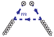
Refer to caption
Figure 8: Feynman diagram for the massive quark beam function at one loop.

The matching coefficient Qgsubscript𝑄𝑔\mathcal{I}_{Qg} generating a massive beam function from a gluon splitting is calculated at 𝒪(αs)𝒪subscript𝛼𝑠\mathcal{O}(\alpha_{s}) in sec. B.1 and corresponds to the diagram shown in fig. 8. The result reads (pT2=|pT|2superscriptsubscript𝑝𝑇2superscriptsubscript𝑝𝑇2p_{T}^{2}=|\vec{p}_{T}|^{2})

Qg(pT,m,z)=Q¯g(pT,m,z)=αsTF4π2θ(z)θ(1z)2pT2+m2[Pqg(z)+2m2z(1z)pT2+m2]+𝒪(αs2),subscript𝑄𝑔subscript𝑝𝑇𝑚𝑧subscript¯𝑄𝑔subscript𝑝𝑇𝑚𝑧subscript𝛼𝑠subscript𝑇𝐹4superscript𝜋2𝜃𝑧𝜃1𝑧2superscriptsubscript𝑝𝑇2superscript𝑚2delimited-[]subscript𝑃𝑞𝑔𝑧2superscript𝑚2𝑧1𝑧superscriptsubscript𝑝𝑇2superscript𝑚2𝒪superscriptsubscript𝛼𝑠2\displaystyle\mathcal{I}_{Qg}(\vec{p}_{T},m,z)=\mathcal{I}_{\bar{Q}g}(\vec{p}_{T},m,z)=\frac{\alpha_{s}T_{F}}{4\pi^{2}}\,\theta(z)\,\theta(1-z)\,\frac{2}{p_{T}^{2}+m^{2}}\biggl{[}P_{qg}(z)+\frac{2m^{2}z(1-z)}{p_{T}^{2}+m^{2}}\biggr{]}+\mathcal{O}(\alpha_{s}^{2})\,, (63)

with the splitting function

Pqg(z)=z2+(1z)2.subscript𝑃𝑞𝑔𝑧superscript𝑧2superscript1𝑧2\displaystyle P_{qg}(z)=z^{2}+(1-z)^{2}\,. (64)

This result is equivalent to the Fourier transform of the mass-dependent matching functions 𝒞h/Gsubscript𝒞𝐺\mathcal{C}_{h/G} in ref. Nadolsky:2002jr . After performing an appropriate crossing it also agrees with the massive final-state splitting functions Catani:2000ef ; Kang:2016ofv or fragmenting jet function Bauer:2013bza .
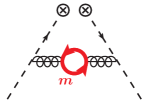
Refer to caption
Refer to caption
Refer to caption
Figure 9: Secondary massive quark corrections for the light-quark beam function at 𝒪(αs2)𝒪superscriptsubscript𝛼𝑠2\mathcal{O}(\alpha_{s}^{2}). In addition, also the wave-function renormalization correction and the mirror diagrams for (b) and (c) have to be included.

The contributions from secondary massive quarks to the matching coefficient qqsubscript𝑞𝑞\mathcal{I}_{qq} are computed in sec. B.3 at 𝒪(αs2)𝒪superscriptsubscript𝛼𝑠2\mathcal{O}(\alpha_{s}^{2}). The corresponding diagrams are shown in fig. 9. The result is given by

qq(2,h)(pT,m,z,μ,νω)superscriptsubscript𝑞𝑞2subscript𝑝𝑇𝑚𝑧𝜇𝜈𝜔\displaystyle\mathcal{I}_{qq}^{(2,h)}\Bigl{(}\vec{p}_{T},m,z,\mu,\frac{\nu}{\omega}\Bigr{)}
=θ(z)CF{δ(2)(pT)δ(1z)[(83Lm2+809Lm+22427)lnνω+2Lm2+(23+8π29)Lm\displaystyle\quad=\theta(z)C_{F}\biggl{\{}\delta^{(2)}(\vec{p}_{T})\,\delta(1-z)\biggl{[}\Bigl{(}\frac{8}{3}L_{m}^{2}+\frac{80}{9}L_{m}+\frac{224}{27}\Bigr{)}\ln\frac{\nu}{\omega}+2L_{m}^{2}+\Bigl{(}\frac{2}{3}+\frac{8\pi^{2}}{9}\Bigr{)}L_{m}
+7318+20π2278ζ33]\displaystyle\qquad\quad+\frac{73}{18}+\frac{20\pi^{2}}{27}-\frac{8\zeta_{3}}{3}\biggr{]}
+169πpT2[0(1z)δ(1z)lnνω][5+12m^2+3c(12m^2)lnc+1c1]169𝜋superscriptsubscript𝑝𝑇2delimited-[]subscript01𝑧𝛿1𝑧𝜈𝜔delimited-[]512superscript^𝑚23𝑐12superscript^𝑚2𝑐1𝑐1\displaystyle\qquad+\frac{16}{9\pi p_{T}^{2}}\Bigl{[}\mathcal{L}_{0}(1-z)-\delta(1-z)\ln\frac{\nu}{\omega}\Bigr{]}\Bigl{[}-5+12\hat{m}^{2}+3c(1-2\hat{m}^{2})\ln\frac{c+1}{c-1}\Bigr{]}
+169πpT2θ(1z)[32d(1z)[(1+z2)(1+2m^2z)+4m^4z2(5+6z5z2)]lnd+1d1\displaystyle\qquad+\frac{16}{9\pi p_{T}^{2}}\theta(1-z)\biggl{[}\frac{3}{2d(1-z)}\bigl{[}(1+z^{2})(1+2\hat{m}^{2}z)+4\hat{m}^{4}z^{2}(-5+6z-5z^{2})\bigr{]}\ln\frac{d+1}{d-1}
3c(12m^2)1zlnc+1c1+1+4z+3m^2(4+z5z2)]}\displaystyle\qquad\quad-\frac{3c(1-2\hat{m}^{2})}{1-z}\ln\frac{c+1}{c-1}+1+4z+3\hat{m}^{2}(-4+z-5z^{2})\biggr{]}\biggr{\}}
+43Lmqq(1)(pT,z,μ,νω),43subscript𝐿𝑚superscriptsubscript𝑞𝑞1subscript𝑝𝑇𝑧𝜇𝜈𝜔\displaystyle\qquad+\frac{4}{3}L_{m}\,\mathcal{I}_{qq}^{(1)}\Bigl{(}\vec{p}_{T},z,\mu,\frac{\nu}{\omega}\Bigr{)}\,, (65)

where

m^mpT,c=1+4m^2,d=1+4m^2z,formulae-sequence^𝑚𝑚subscript𝑝𝑇formulae-sequence𝑐14superscript^𝑚2𝑑14superscript^𝑚2𝑧\displaystyle\hat{m}\equiv\frac{m}{p_{T}}\,,\qquad c=\sqrt{1+4\hat{m}^{2}}\,,\qquad d=\sqrt{1+4\hat{m}^{2}z}\,, (66)

and the one-loop term qq(1)superscriptsubscript𝑞𝑞1\mathcal{I}_{qq}^{(1)} is given in eq. (119). Here n(1z)subscript𝑛1𝑧\mathcal{L}_{n}(1-z) denotes the standard plus distribution as defined in appendix D.

In the (nl+1)subscript𝑛𝑙1(n_{l}+1)-flavor scheme for αssubscript𝛼𝑠\alpha_{s} there is also a correction from a virtual massive quark loop to the flavor-nondiagonal matching coefficient qg(2)subscriptsuperscript2𝑞𝑔\mathcal{I}^{(2)}_{qg}. This contribution is trivial, since it factorizes into a vacuum polarization correction corresponding to the matching of αssubscript𝛼𝑠\alpha_{s} between the (nl)subscript𝑛𝑙(n_{l}) and (nl+1)subscript𝑛𝑙1(n_{l}+1)-flavor schemes, and the one-loop contribution, such that

qg(2,h)(pT,m,z,μ)=43Lmqg(1)(pT,z,μ),superscriptsubscript𝑞𝑔2subscript𝑝𝑇𝑚𝑧𝜇43subscript𝐿𝑚superscriptsubscript𝑞𝑔1subscript𝑝𝑇𝑧𝜇\displaystyle\mathcal{I}_{qg}^{(2,h)}(\vec{p}_{T},m,z,\mu)=\frac{4}{3}L_{m}\,\mathcal{I}_{qg}^{(1)}(\vec{p}_{T},z,\mu)\,, (67)

with qg(1)superscriptsubscript𝑞𝑔1\mathcal{I}_{qg}^{(1)} given in eq. (118). In the (nl)subscript𝑛𝑙(n_{l})-flavor scheme for αssubscript𝛼𝑠\alpha_{s} the qg(2,h)superscriptsubscript𝑞𝑔2\mathcal{I}_{qg}^{(2,h)} contribution vanishes.

The contributions from a massive flavor to the beam function anomalous dimensions are

γB(2,h)(νω)superscriptsubscript𝛾𝐵2𝜈𝜔\displaystyle\gamma_{B}^{(2,h)}\Bigl{(}\frac{\nu}{\omega}\Bigr{)} =CF(1609lnνω4316π29),absentsubscript𝐶𝐹1609𝜈𝜔4316superscript𝜋29\displaystyle=C_{F}\,\biggl{(}-\frac{160}{9}\ln\frac{\nu}{\omega}-\frac{4}{3}-\frac{16\pi^{2}}{9}\biggr{)}\,,
γν,B(2,h)(pT,m,μ)superscriptsubscript𝛾𝜈𝐵2subscript𝑝𝑇𝑚𝜇\displaystyle\gamma_{\nu,B}^{(2,h)}(\vec{p}_{T},m,\mu) =CF{163Lm0(pT,μ)+δ(2)(pT)(83Lm2+809Lm+22427)\displaystyle=C_{F}\,\biggl{\{}-\frac{16}{3}L_{m}\mathcal{L}_{0}(\vec{p}_{T},\mu)+\delta^{(2)}(\vec{p}_{T})\Bigl{(}\frac{8}{3}L_{m}^{2}+\frac{80}{9}L_{m}+\frac{224}{27}\Bigr{)}
+169πpT2[512m^23c(12m^2)lnc+1c1]}.\displaystyle\quad+\frac{16}{9\pi p_{T}^{2}}\biggl{[}5-12\hat{m}^{2}-3c(1-2\hat{m}^{2})\ln\frac{c+1}{c-1}\biggr{]}\biggr{\}}\,. (68)

The 0(pT,μ)subscript0subscript𝑝𝑇𝜇\mathcal{L}_{0}(\vec{p}_{T},\mu) distribution is defined in appendix D. The μ𝜇\mu anomalous dimension here is the same as for a massless quark flavor, γB(2,h)=γB(2,l)superscriptsubscript𝛾𝐵2superscriptsubscript𝛾𝐵2𝑙\gamma_{B}^{(2,h)}=\gamma_{B}^{(2,l)} [see eq. (A.2.1)]. The rapidity anomalous dimension is explicitly mass dependent and only reproduces the result for a massless flavor in the limit mpTmuch-less-than𝑚subscript𝑝𝑇m\ll p_{T}.

4.2.2 Virtuality-dependent beam function coefficients

The massive quark-gluon virtuality beam function matching coefficient at 𝒪(αs)𝒪subscript𝛼𝑠\mathcal{O}(\alpha_{s}) shown in fig. 8 is given by

Qg(t,m,z)=αsTF4πθ(t)θ(z)θ[t(1z)zm2]2t[Pqg(z)+2m2z2t]+𝒪(αs2).subscript𝑄𝑔𝑡𝑚𝑧subscript𝛼𝑠subscript𝑇𝐹4𝜋𝜃𝑡𝜃𝑧𝜃delimited-[]𝑡1𝑧𝑧superscript𝑚22𝑡delimited-[]subscript𝑃𝑞𝑔𝑧2superscript𝑚2superscript𝑧2𝑡𝒪superscriptsubscript𝛼𝑠2\displaystyle\mathcal{I}_{Qg}(t,m,z)=\frac{\alpha_{s}T_{F}}{4\pi}\,\theta(t)\,\theta(z)\,\theta\biggl{[}\frac{t(1-z)}{z}-m^{2}\biggr{]}\,\frac{2}{t}\biggl{[}P_{qg}(z)+\frac{2m^{2}z^{2}}{t}\biggr{]}+\mathcal{O}(\alpha_{s}^{2})\,. (69)

The contributions from secondary massive quarks to the light-quark coefficient at 𝒪(αs2)𝒪superscriptsubscript𝛼𝑠2\mathcal{O}(\alpha_{s}^{2}) as shown in fig. 9 are given by

qq(2,h)(t,m,z,μ,νω)superscriptsubscript𝑞𝑞2𝑡𝑚𝑧𝜇𝜈𝜔\displaystyle\mathcal{I}_{qq}^{(2,h)}\Bigl{(}t,m,z,\mu,\frac{\nu}{\omega}\Bigr{)}
=θ(z)CF{δ(t)δ(1z)[(83Lm2+809Lm+22427)lnνω+2Lm2+(23+8π29)Lm\displaystyle\quad=\theta(z)C_{F}\biggl{\{}\delta(t)\,\delta(1-z)\biggl{[}\Bigl{(}\frac{8}{3}L_{m}^{2}+\frac{80}{9}L_{m}+\frac{224}{27}\Bigr{)}\ln\frac{\nu}{\omega}+2L_{m}^{2}+\Bigl{(}\frac{2}{3}+\frac{8\pi^{2}}{9}\Bigr{)}L_{m}
+7318+20π2278ζ33]\displaystyle\qquad\quad+\frac{73}{18}+\frac{20\pi^{2}}{27}-\frac{8\zeta_{3}}{3}\biggr{]}
+θ(t4m2z1z)89t(1z)[3u[(1+z2)(12m^t2z)4m^t4z2(23z+5z2)]lnuvu+v\displaystyle\qquad+\theta\biggl{(}t-\frac{4m^{2}z}{1-z}\biggr{)}\frac{8}{9t(1-z)}\biggl{[}-\frac{3}{u}\Bigl{[}(1+z^{2})(1-2\hat{m}_{t}^{2}z)-4\hat{m}_{t}^{4}z^{2}(2-3z+5z^{2})\Bigr{]}\ln\frac{u-v}{u+v}
2v[43z+4z2+z(1121z+29z215z3)1zm^t2]]}+43Lmqq(1)(t,z,μ),\displaystyle\qquad\quad-2v\Bigl{[}4-3z+4z^{2}+\frac{z(11-21z+29z^{2}-15z^{3})}{1-z}\,\hat{m}_{t}^{2}\Bigr{]}\biggr{]}\biggr{\}}+\frac{4}{3}L_{m}\,\mathcal{I}_{qq}^{(1)}(t,z,\mu)\,, (70)

with

m^t=mtu=14m^t2z,v=14m^t2z1z,formulae-sequencesubscript^𝑚𝑡𝑚𝑡formulae-sequence𝑢14superscriptsubscript^𝑚𝑡2𝑧𝑣14superscriptsubscript^𝑚𝑡2𝑧1𝑧\displaystyle\hat{m}_{t}=\frac{m}{\sqrt{t}}\,\qquad u=\sqrt{1-4\hat{m}_{t}^{2}z}\,,\qquad v=\sqrt{1-\frac{4\hat{m}_{t}^{2}z}{1-z}}\,, (71)

and the one-loop term qq(1)superscriptsubscript𝑞𝑞1\mathcal{I}_{qq}^{(1)} is given in eq. (123).

In the (nl+1)subscript𝑛𝑙1(n_{l}+1)-flavor scheme for αssubscript𝛼𝑠\alpha_{s} there is also the analogous contribution to eq. (67) to the flavor-nondiagonal coefficient

qg(2,h)(t,m,z,μ)=43Lmqg(1)(t,z,μ),superscriptsubscript𝑞𝑔2𝑡𝑚𝑧𝜇43subscript𝐿𝑚superscriptsubscript𝑞𝑔1𝑡𝑧𝜇\displaystyle\mathcal{I}_{qg}^{(2,h)}(t,m,z,\mu)=\frac{4}{3}L_{m}\,\mathcal{I}_{qg}^{(1)}(t,z,\mu)\,, (72)

with qg(1)superscriptsubscript𝑞𝑔1\mathcal{I}_{qg}^{(1)} given in eq. (123). In the (nl)subscript𝑛𝑙(n_{l})-flavor scheme for αssubscript𝛼𝑠\alpha_{s} the qg(2,h)superscriptsubscript𝑞𝑔2\mathcal{I}_{qg}^{(2,h)} contribution vanishes.

The contribution from the massive flavor to the μ𝜇\mu anomalous dimension at 𝒪(αs2)𝒪superscriptsubscript𝛼𝑠2\mathcal{O}(\alpha_{s}^{2}) is given by

γB,m(2,h)(t,νω)subscriptsuperscript𝛾2𝐵𝑚𝑡𝜈𝜔\displaystyle\gamma^{(2,h)}_{B,m}\Bigl{(}t,\frac{\nu}{\omega}\Bigr{)} =CFδ(t)(1609lnνω4316π29).absentsubscript𝐶𝐹𝛿𝑡1609𝜈𝜔4316superscript𝜋29\displaystyle=C_{F}\,\delta(t)\biggl{(}-\frac{160}{9}\ln\frac{\nu}{\omega}-\frac{4}{3}-\frac{16\pi^{2}}{9}\biggr{)}\,. (73)

We emphasize that the massive quark contribution to the μ𝜇\mu anomalous dimension is not the same as for a massless flavor, but is in fact the same as for the TMD beam function in eq. (4.2.1). This is required by consistency with the large mass limit Q𝒯,qTmmuch-less-than𝑄𝒯subscript𝑞𝑇𝑚Q{\mathcal{T}},q_{T}\ll m, where the massive flavor can only contribute to the (local) running of the common current operators, which are independent of the measurement. Only in combination with the soft mass-mode function Hssubscript𝐻𝑠H_{s} and the soft function, the combined μ𝜇\mu evolution above the mass scale is the same as for nl+1subscript𝑛𝑙1n_{l}+1 massless flavors as discussed in eq. (3.2).

The secondary massive quarks introduce rapidity divergences and associated logarithms also in the virtuality-dependent beam function. The ν𝜈\nu anomalous dimension induced by the secondary massive effects is the same as for the collinear mass-mode function, see eq. (34), given in eq. (4.1.2).

4.2.3 PDF matching coefficients

The matching coefficients relating the PDFs in the (nl+1)subscript𝑛𝑙1(n_{l}+1) and the (nl)subscript𝑛𝑙(n_{l})-flavor scheme are all known at two loops Buza:1996wv and partially beyond (see e.g. refs. Ablinger:2014nga ; Ablinger:2014vwa ; Ablinger:2014lka and references therein). The matching coefficient for a primary massive quark originating from an initial-state gluon at 𝒪(αs)𝒪subscript𝛼𝑠\mathcal{O}(\alpha_{s}) is

Qg(m,z,μ)=αsTF4πθ(1z)θ(z) 2Pqg(z)Lm+𝒪(αs2).subscript𝑄𝑔𝑚𝑧𝜇subscript𝛼𝑠subscript𝑇𝐹4𝜋𝜃1𝑧𝜃𝑧2subscript𝑃𝑞𝑔𝑧subscript𝐿𝑚𝒪superscriptsubscript𝛼𝑠2\displaystyle\mathcal{M}_{Qg}(m,z,\mu)=-\frac{\alpha_{s}T_{F}}{4\pi}\,\theta(1-z)\theta(z)\,2P_{qg}(z)L_{m}+\mathcal{O}(\alpha_{s}^{2})\,. (74)

The matching coefficient coming from secondary massive quark corrections to the light-quark PDFs reads up to 𝒪(αs2)𝒪superscriptsubscript𝛼𝑠2\mathcal{O}(\alpha_{s}^{2})

qq(m,z,μ)subscript𝑞𝑞𝑚𝑧𝜇\displaystyle\mathcal{M}_{qq}(m,z,\mu) =1+αs2CFTF16π2θ(z){0(1z)(83Lm2+809Lm+22427)\displaystyle=1+\frac{\alpha_{s}^{2}C_{F}T_{F}}{16\pi^{2}}\,\theta(z)\biggl{\{}\mathcal{L}_{0}(1-z)\biggl{(}\frac{8}{3}L_{m}^{2}+\frac{80}{9}L_{m}+\frac{224}{27}\biggr{)}
+δ(1z)[2Lm2+(23+8π29)Lm+7318+20π2278ζ33]𝛿1𝑧delimited-[]2superscriptsubscript𝐿𝑚2238superscript𝜋29subscript𝐿𝑚731820superscript𝜋2278subscript𝜁33\displaystyle\qquad+\delta(1-z)\biggl{[}2L_{m}^{2}+\left(\frac{2}{3}+\frac{8\pi^{2}}{9}\right)L_{m}+\frac{73}{18}+\frac{20\pi^{2}}{27}-\frac{8\zeta_{3}}{3}\biggr{]}
+θ(1z)[43Lm2(1+z)+Lm(89889z+831+z21zlnz)+231+z21zln2z\displaystyle\qquad+\theta(1-z)\ \biggl{[}-\frac{4}{3}L_{m}^{2}(1+z)+L_{m}\biggl{(}\frac{8}{9}-\frac{88}{9}z+\frac{8}{3}\frac{1+z^{2}}{1-z}\,\ln z\biggr{)}+\frac{2}{3}\frac{1+z^{2}}{1-z}\,\ln^{2}z
+lnz1z(449163z+449z2)+442726827z]}+𝒪(αs3).\displaystyle\qquad+\frac{\ln z}{1-z}\biggl{(}\frac{44}{9}-\frac{16}{3}z+\frac{44}{9}z^{2}\biggr{)}+\frac{44}{27}-\frac{268}{27}z\biggr{]}\biggr{\}}+\mathcal{O}(\alpha_{s}^{3})\,. (75)

The matching coefficient between the gluon PDF in the (nl)subscript𝑛𝑙(n_{l}) and (nl+1)subscript𝑛𝑙1(n_{l}+1)-flavor schemes at 𝒪(αs)𝒪subscript𝛼𝑠\mathcal{O}(\alpha_{s}), which is also required for Drell-Yan at 𝒪(αs2)𝒪superscriptsubscript𝛼𝑠2\mathcal{O}(\alpha_{s}^{2}), is equivalent to the matching relation for αssubscript𝛼𝑠\alpha_{s}

gg(m,z,μ)=δ(1z)+αsTF4πδ(1z)43Lm+𝒪(αs2).subscript𝑔𝑔𝑚𝑧𝜇𝛿1𝑧subscript𝛼𝑠subscript𝑇𝐹4𝜋𝛿1𝑧43subscript𝐿𝑚𝒪superscriptsubscript𝛼𝑠2\displaystyle\mathcal{M}_{gg}(m,z,\mu)=\delta(1-z)+\frac{\alpha_{s}T_{F}}{4\pi}\,\delta(1-z)\,\frac{4}{3}L_{m}+\mathcal{O}(\alpha_{s}^{2})\,. (76)

Note that taking into account the nondiagonal evolution of the PDFs the known 𝒪(αs2)𝒪superscriptsubscript𝛼𝑠2\mathcal{O}(\alpha_{s}^{2}) corrections for all matching factors ijsubscript𝑖𝑗\mathcal{M}_{ij} become relevant at NNLL.

4.3 Soft and collinear-soft functions

Here we give all massive quark corrections at 𝒪(αs2)𝒪superscriptsubscript𝛼𝑠2\mathcal{O}(\alpha_{s}^{2}) to the soft and csoft functions. They arise exclusively from secondary radiation. Note that the soft functions satisfy Casimir scaling at this order and can be thus applied also to color-singlet production in gluon-fusion by replacing an overall CFCAsubscript𝐶𝐹subscript𝐶𝐴C_{F}\to C_{A}.

4.3.1 TMD soft function

Refer to caption
Refer to caption
Figure 10: Corrections from secondary massive quarks to the (c)soft function. Also the mirror diagrams need to be included.

The contributions from secondary massive quarks to the TMD soft function, which appears in eq. (2.4) for qTmsimilar-tosubscript𝑞𝑇𝑚q_{T}\sim m, are calculated in app. B.4 at 𝒪(αs2)𝒪superscriptsubscript𝛼𝑠2\mathcal{O}(\alpha_{s}^{2}) and correspond to the diagrams shown in fig. 10. The result reads

S(2,h)(pT,m,μ,ν)superscript𝑆2subscript𝑝𝑇𝑚𝜇𝜈\displaystyle S^{(2,h)}(\vec{p}_{T},m,\mu,\nu) =CF{δ(2)(pT)[(163Lm21609Lm44827)lnνμ+89Lm3+409Lm2\displaystyle=C_{F}\,\biggl{\{}\delta^{(2)}(\vec{p}_{T})\biggl{[}\Bigl{(}-\frac{16}{3}L_{m}^{2}-\frac{160}{9}L_{m}-\frac{448}{27}\Bigr{)}\ln\frac{\nu}{\mu}+\frac{8}{9}L_{m}^{3}+\frac{40}{9}L_{m}^{2}
+(448274π29)Lm+6562710π22756ζ39]\displaystyle\qquad+\Bigl{(}\frac{448}{27}-\frac{4\pi^{2}}{9}\Bigr{)}L_{m}+\frac{656}{27}-\frac{10\pi^{2}}{27}-\frac{56\zeta_{3}}{9}\biggr{]}
+169πpT2[2[5+12m^2+3c(12m^2)lnc+1c1]lnνm\displaystyle\quad+\frac{16}{9\pi p_{T}^{2}}\biggl{[}2\Bigl{[}-5+12\hat{m}^{2}+3c(1-2\hat{m}^{2})\ln\frac{c+1}{c-1}\Bigr{]}\ln\frac{\nu}{m}
+3c(12m^2)[Li2((c1)2(c+1)2)+2lnc+1c1lnm^(c+1)2cπ26]3𝑐12superscript^𝑚2delimited-[]subscriptLi2superscript𝑐12superscript𝑐122𝑐1𝑐1^𝑚𝑐12𝑐superscript𝜋26\displaystyle\qquad+3c(1-2\hat{m}^{2})\biggl{[}\textrm{Li}_{2}\biggl{(}\frac{(c-1)^{2}}{(c+1)^{2}}\biggr{)}+2\ln\frac{c+1}{c-1}\ln\frac{\hat{m}(c+1)}{2c}-\frac{\pi^{2}}{6}\biggr{]}
+c(516m^2)lnc+1c1+8m^2]}+43LmS(1)(pT,μ,ν),\displaystyle\qquad+c(5-16\hat{m}^{2})\ln\frac{c+1}{c-1}+8\hat{m}^{2}\biggr{]}\biggr{\}}+\frac{4}{3}L_{m}\,S^{(1)}(\vec{p}_{T},\mu,\nu)\,, (77)

where m^=m/pT^𝑚𝑚subscript𝑝𝑇\hat{m}=m/p_{T} and c=1+4m^2𝑐14superscript^𝑚2c=\sqrt{1+4\hat{m}^{2}} as in eq. (66) and the one-loop soft function S(1)superscript𝑆1S^{(1)} given in eq. (126).

The massive quark contributions to the anomalous dimensions of the soft function are

γS(2,h)(pT,μ,ν)superscriptsubscript𝛾𝑆2subscript𝑝𝑇𝜇𝜈\displaystyle\gamma_{S}^{(2,h)}(\vec{p}_{T},\mu,\nu) =CF(3209lnνμ44827+8π29),absentsubscript𝐶𝐹3209𝜈𝜇448278superscript𝜋29\displaystyle=C_{F}\,\biggl{(}\frac{320}{9}\ln\frac{\nu}{\mu}-\frac{448}{27}+\frac{8\pi^{2}}{9}\biggr{)}\,,
γν,S(2,h)(pT,m,μ)superscriptsubscript𝛾𝜈𝑆2subscript𝑝𝑇𝑚𝜇\displaystyle\gamma_{\nu,S}^{(2,h)}(\vec{p}_{T},m,\mu) =CF{323Lm0(pT,μ)+δ(2)(pT)(163Lm21609Lm44827)\displaystyle=C_{F}\,\biggl{\{}\frac{32}{3}L_{m}\mathcal{L}_{0}(\vec{p}_{T},\mu)+\delta^{(2)}(\vec{p}_{T})\biggl{(}-\frac{16}{3}L_{m}^{2}-\frac{160}{9}L_{m}-\frac{448}{27}\biggr{)}
+329πpT2[5+12m^2+3c(12m^2)lnc+1c1]}.\displaystyle\quad+\frac{32}{9\pi p_{T}^{2}}\biggl{[}-5+12\hat{m}^{2}+3c(1-2\hat{m}^{2})\ln\frac{c+1}{c-1}\biggr{]}\biggr{\}}\,. (78)

The μ𝜇\mu anomalous dimension here is the same as for an additional massless flavor, γS(2,h)=γS(2,l)superscriptsubscript𝛾𝑆2superscriptsubscript𝛾𝑆2𝑙\gamma_{S}^{(2,h)}=\gamma_{S}^{(2,l)} [see eq. (A.3.1)]. The rapidity anomalous dimension is explicitly mass dependent and only reduces to the result for a massless flavor in the limit mpTmuch-less-than𝑚subscript𝑝𝑇m\ll p_{T}.

4.3.2 Csoft function for beam thrust

The csoft function is a matching coefficient between an eikonal matrix element in the nl+1subscript𝑛𝑙1n_{l}+1 and nlsubscript𝑛𝑙n_{l} flavor theories appearing for the hierarchy 𝒯mQ𝒯much-less-than𝒯𝑚much-less-than𝑄𝒯{\mathcal{T}}\ll m\ll\sqrt{Q{\mathcal{T}}} in eq. (3.3). The relevant diagrams at 𝒪(αs2)𝒪superscriptsubscript𝛼𝑠2\mathcal{O}(\alpha_{s}^{2}) are shown in fig. 10 and are calculated in sec. B.5. The result is given by

𝒮c(,m,μ,ν)subscript𝒮𝑐𝑚𝜇𝜈\displaystyle\mathcal{S}_{c}(\ell,m,\mu,\nu) =δ()+αs2CFTF16π2{νμ20(νμ2)(83Lm2+809Lm+22427)\displaystyle=\delta(\ell)+\frac{\alpha_{s}^{2}C_{F}T_{F}}{16\pi^{2}}\biggl{\{}\frac{\nu}{\mu^{2}}\mathcal{L}_{0}\Bigl{(}\frac{\ell\,\nu}{\mu^{2}}\Bigr{)}\Bigl{(}\frac{8}{3}L_{m}^{2}+\frac{80}{9}L_{m}+\frac{224}{27}\Bigr{)} (79)
+δ()[89Lm3409Lm2+(44827+4π29)Lm65627+10π227+56ζ39]}+𝒪(αs3).\displaystyle\quad+\delta(\ell)\biggl{[}-\frac{8}{9}L_{m}^{3}-\frac{40}{9}L_{m}^{2}+\Bigl{(}-\frac{448}{27}+\frac{4\pi^{2}}{9}\Bigr{)}L_{m}-\frac{656}{27}+\frac{10\pi^{2}}{27}+\frac{56\zeta_{3}}{9}\biggr{]}\biggr{\}}+\mathcal{O}(\alpha_{s}^{3}).

We can see that with the scale choices μmsimilar-to𝜇𝑚\mu\sim m and νμ2/m2/𝒯similar-to𝜈superscript𝜇2similar-tosuperscript𝑚2𝒯\nu\sim\mu^{2}/\ell\sim m^{2}/{\mathcal{T}} all large logarithms (including the implicit one inside the plus distribution) are minimized. The μ𝜇\mu anomalous dimensions of the csoft matching function is given by

γ𝒮c(,m,μ,ν)subscript𝛾subscript𝒮𝑐𝑚𝜇𝜈\displaystyle\gamma_{\mathcal{S}_{c}}(\ell,m,\mu,\nu) =αs2CFTF16π2[νμ20(νμ2)(323Lm+1609)+δ()(448278π29)]+𝒪(αs3).absentsuperscriptsubscript𝛼𝑠2subscript𝐶𝐹subscript𝑇𝐹16superscript𝜋2delimited-[]𝜈superscript𝜇2subscript0𝜈superscript𝜇2323subscript𝐿𝑚1609𝛿448278superscript𝜋29𝒪superscriptsubscript𝛼𝑠3\displaystyle=\frac{\alpha_{s}^{2}C_{F}T_{F}}{16\pi^{2}}\biggl{[}-\frac{\nu}{\mu^{2}}\mathcal{L}_{0}\Bigl{(}\frac{\ell\,\nu}{\mu^{2}}\Bigr{)}\Bigl{(}\frac{32}{3}L_{m}+\frac{160}{9}\Bigr{)}+\delta(\ell)\Bigl{(}\frac{448}{27}-\frac{8\pi^{2}}{9}\Bigr{)}\biggr{]}+\mathcal{O}(\alpha_{s}^{3})\,. (80)

The ν𝜈\nu anomalous dimension is the same as for the collinear mass mode function in eq. (4.1.2), γν,𝒮c=γν,Hcsubscript𝛾𝜈subscript𝒮𝑐subscript𝛾𝜈subscript𝐻𝑐\gamma_{\nu,\mathcal{S}_{c}}=\gamma_{\nu,H_{c}}.

4.3.3 (Beam) thrust soft function

The secondary massive quark corrections to the (beam) thrust soft function at 𝒪(αs2)𝒪superscriptsubscript𝛼𝑠2\mathcal{O}(\alpha_{s}^{2}) were calculated in ref. Gritschacher:2013tza and are given by

S(2,h)(,m,μ)superscript𝑆2𝑚𝜇\displaystyle S^{(2,h)}(\ell,m,\mu) =CF{1μ0(μ)(163Lm2+1609Lm+44827)\displaystyle=C_{F}\,\biggl{\{}\frac{1}{\mu}\mathcal{L}_{0}\Bigl{(}\frac{\ell}{\mu}\Bigr{)}\biggl{(}\frac{16}{3}L_{m}^{2}+\frac{160}{9}L_{m}+\frac{448}{27}\biggr{)}
+δ()[89Lm3409Lm2+(44827+4π29)Lm65627+10π227+569ζ3]𝛿delimited-[]89superscriptsubscript𝐿𝑚3409superscriptsubscript𝐿𝑚2448274superscript𝜋29subscript𝐿𝑚6562710superscript𝜋227569subscript𝜁3\displaystyle\quad+\delta(\ell)\biggl{[}-\frac{8}{9}L_{m}^{3}-\frac{40}{9}L_{m}^{2}+\Bigl{(}-\frac{448}{27}+\frac{4\pi^{2}}{9}\Bigr{)}L_{m}-\frac{656}{27}+\frac{10\pi^{2}}{27}+\frac{56}{9}\zeta_{3}\biggr{]}
+θ(2m)1[643Li2(w1w+1)+163ln21w1+w643ln1w1+wlnm^\displaystyle\quad+\theta(\ell-2m)\frac{1}{\ell}\biggl{[}\frac{64}{3}\,\textrm{Li}_{2}\Bigl{(}\frac{w-1}{w+1}\Bigr{)}+\frac{16}{3}\ln^{2}\frac{1-w}{1+w}-\frac{64}{3}\ln\frac{1-w}{1+w}\ln\hat{m}_{\ell}
1609ln1w1+ww(89627+25627m^2)+16π29]}\displaystyle\qquad-\frac{160}{9}\ln\frac{1-w}{1+w}-w\Bigl{(}\frac{896}{27}+\frac{256}{27}\hat{m}_{\ell}^{2}\Bigr{)}+\frac{16\pi^{2}}{9}\biggr{]}\biggr{\}}
+ΔSτ(,m)+43LmS(1)(,μ),Δsubscript𝑆𝜏𝑚43subscript𝐿𝑚superscript𝑆1𝜇\displaystyle\quad+\Delta S_{\tau}(\ell,m)+\frac{4}{3}L_{m}\,S^{(1)}(\ell,\mu)\,, (81)

where

m^m,w=14m^2,formulae-sequencesubscript^𝑚𝑚𝑤14superscriptsubscript^𝑚2\displaystyle\hat{m}_{\ell}\equiv\frac{m}{\ell}\,,\qquad w=\sqrt{1-4\hat{m}_{\ell}^{2}}\,, (82)

and the one-loop soft function S(1)superscript𝑆1S^{(1)} is given in eq. (129). The term ΔSτ(,m)Δsubscript𝑆𝜏𝑚\Delta S_{\tau}(\ell,m) contains the correction from two real final-state emissions entering two opposite hemispheres, which vanishes both for mmuch-less-than𝑚\ell\ll m and mmuch-less-than𝑚m\ll\ell and is currently only known numerically. The integral expression for this numerically small contribution is given in eq. (61) of ref. Gritschacher:2013tza , and a precise parametrization can be found in ref. Pietrulewicz:2014qza .

The massive quark contribution to the anomalous dimension is the same as for a massless flavor, γS(2,h)(,μ)=γS(2,l)(,μ)superscriptsubscript𝛾𝑆2𝜇superscriptsubscript𝛾𝑆2𝑙𝜇\gamma_{S}^{(2,h)}(\ell,\mu)=\gamma_{S}^{(2,l)}(\ell,\mu), given in eq. (A.3.2).

4.4 Small and large mass limits

In secs. 2.6 and 3.5 we explained how the ingredients in the factorization theorems for different hierarchies are related to each other. Here we verify these relations for the beam and soft functions up to 𝒪(αs2)𝒪superscriptsubscript𝛼𝑠2\mathcal{O}(\alpha_{s}^{2}). We also scrutinize the numerical impact of the power corrections for these functions. We focus in particular on the 𝒪(m2/qT2)𝒪superscript𝑚2superscriptsubscript𝑞𝑇2\mathcal{O}(m^{2}/q_{T}^{2}) corrections the qTsubscript𝑞𝑇q_{T} spectrum for b𝑏b quarks, which are contained in the factorization theorem eq. (2.4) for qTmsimilar-tosubscript𝑞𝑇𝑚q_{T}\sim m but not in the massless limit for mqTmuch-less-than𝑚subscript𝑞𝑇m\ll q_{T} in eq. (2.5), as these are phenomenologically important hierarchies for b𝑏b-quark mass effects at the LHC.

For the numerical results we use the MMHT2014 NNLO PDFs Harland-Lang:2014zoa and evaluate the contributions for μ=mb=4.8𝜇subscript𝑚𝑏4.8\mu=m_{b}=4.8 GeV, ω=mZ𝜔subscript𝑚𝑍\omega=m_{Z}, and Ecm=13subscript𝐸cm13E_{\rm cm}=13 TeV. The main qualitative features of the results do not depend on these specific input parameters.

4.4.1 Limiting behavior for qTsubscript𝑞𝑇q_{T}

We first consider the primary mass effects at one loop, which are encoded in the TMD beam function matching coefficient Qg(1)superscriptsubscript𝑄𝑔1\mathcal{I}_{Qg}^{(1)} in eq. (63). In the limit pTmmuch-less-thansubscript𝑝𝑇𝑚p_{T}\ll m the primary massive quarks decouple, which is manifest in the result,

Qg(1)(pT,m,z)=𝒪(pT2m2).superscriptsubscript𝑄𝑔1subscript𝑝𝑇𝑚𝑧𝒪superscriptsubscript𝑝𝑇2superscript𝑚2\displaystyle\mathcal{I}_{Qg}^{(1)}(\vec{p}_{T},m,z)=\mathcal{O}\Bigl{(}\frac{p_{T}^{2}}{m^{2}}\Bigr{)}\,. (83)

On the other hand, in the opposite limit mpTmuch-less-than𝑚subscript𝑝𝑇m\ll p_{T} it becomes

Qg(1)(pT,m,z)superscriptsubscript𝑄𝑔1subscript𝑝𝑇𝑚𝑧\displaystyle\mathcal{I}_{Qg}^{(1)}(\vec{p}_{T},m,z)
=TFθ(1z)θ(z){2Pqg(z)0(pT,μ)+δ(2)(pT)[2Pqg(z)Lm+4z(1z)]+𝒪(m2pT2)}absentsubscript𝑇𝐹𝜃1𝑧𝜃𝑧2subscript𝑃𝑞𝑔𝑧subscript0subscript𝑝𝑇𝜇superscript𝛿2subscript𝑝𝑇delimited-[]2subscript𝑃𝑞𝑔𝑧subscript𝐿𝑚4𝑧1𝑧𝒪superscript𝑚2superscriptsubscript𝑝𝑇2\displaystyle\quad=T_{F}\,\theta(1-z)\theta(z)\,\Bigl{\{}2P_{qg}(z)\mathcal{L}_{0}(\vec{p}_{T},\mu)+\delta^{(2)}(\vec{p}_{T})\Bigl{[}-2P_{qg}(z)L_{m}+4z(1-z)\Bigr{]}\!+\mathcal{O}\Bigl{(}\frac{m^{2}}{p_{T}^{2}}\Bigr{)}\biggr{\}}
=qg(1)(pT,z,μ)+δ(2)(pT)Qg(1)(m,z,μ)+𝒪(m2pT2),absentsuperscriptsubscript𝑞𝑔1subscript𝑝𝑇𝑧𝜇superscript𝛿2subscript𝑝𝑇superscriptsubscript𝑄𝑔1𝑚𝑧𝜇𝒪superscript𝑚2superscriptsubscript𝑝𝑇2\displaystyle\quad=\mathcal{I}_{qg}^{(1)}(\vec{p}_{T},z,\mu)+\delta^{(2)}(\vec{p}_{T})\mathcal{M}_{Qg}^{(1)}(m,z,\mu)+\mathcal{O}\Bigl{(}\frac{m^{2}}{p_{T}^{2}}\Bigr{)}\,, (84)

confirming that the relation in eq. (25) is satisfied at 𝒪(αs)𝒪subscript𝛼𝑠\mathcal{O}(\alpha_{s}). The massless one-loop matching coefficient qg(1)superscriptsubscript𝑞𝑔1\mathcal{I}_{qg}^{(1)} can be found in eq. (118) and the PDF matching coefficient Qg(1)superscriptsubscript𝑄𝑔1\mathcal{M}_{Qg}^{(1)} in eq. (74). To account for the correct distributive structure in pTsubscript𝑝𝑇\vec{p}_{T} that emerges in the massless limit, one can integrate the expressions with massive quarks and identify the distributions at the cumulant level.
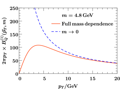
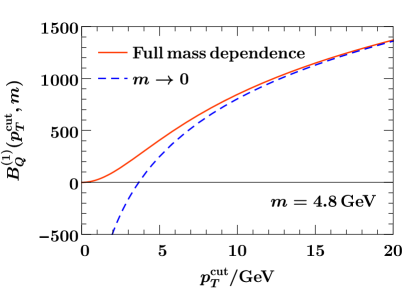
Refer to caption
Refer to caption
Figure 11: Massive b𝑏b-quark beam function (left panel) and its cumulant (right panel) together with its m0𝑚0m\to 0 limit. The input parameters are described in the text.

In fig. 11 we show the result for the massive quark beam function BQ(1)=Qg(1)xfgsubscriptsuperscript𝐵1𝑄subscripttensor-product𝑥subscriptsuperscript1𝑄𝑔subscript𝑓𝑔B^{(1)}_{Q}=\mathcal{I}^{(1)}_{Qg}\otimes_{x}f_{g} at 𝒪(αs)𝒪subscript𝛼𝑠\mathcal{O}(\alpha_{s}) as function of pTsubscript𝑝𝑇p_{T} using the full massive matching coefficient Qg(1)subscriptsuperscript1𝑄𝑔\mathcal{I}^{(1)}_{Qg} (solid orange) and its small mass limit in eq. (4.4.1). Note that the results differential in pTsubscript𝑝𝑇p_{T} are not explicitly μ𝜇\mu-dependent at 𝒪(αs)𝒪subscript𝛼𝑠\mathcal{O}(\alpha_{s}). In the right panel we show the corresponding results for the cumulant

BQ(pTcut,m)|pT|<pTcutd2pTBQ(pT,m),subscript𝐵𝑄superscriptsubscript𝑝𝑇cut𝑚subscriptsubscript𝑝𝑇superscriptsubscript𝑝𝑇cutsuperscriptd2subscript𝑝𝑇subscript𝐵𝑄subscript𝑝𝑇𝑚\displaystyle B_{Q}(p_{T}^{\rm cut},m)\equiv\int_{|\vec{p}_{T}|<p_{T}^{\rm cut}}\textrm{d}^{2}p_{T}\,B_{Q}(\vec{p}_{T},m)\,, (85)

which also includes the δ(2)(pT)superscript𝛿2subscript𝑝𝑇\delta^{(2)}(\vec{p}_{T}) constant contribution. We can see that in both cases the small mass limit is correctly approached for pT(cut)mbmuch-greater-thansuperscriptsubscript𝑝𝑇cutsubscript𝑚𝑏p_{T}^{(\rm cut)}\gg m_{b}, while for pT(cut)mbmuch-less-thansuperscriptsubscript𝑝𝑇cutsubscript𝑚𝑏p_{T}^{(\rm cut)}\ll m_{b} the primary mass effects decouple with the result going to zero. The corrections to the small mass limit become sizeable for pTmbsimilar-tosubscript𝑝𝑇subscript𝑚𝑏p_{T}\sim m_{b} and vanish quite fast for larger pTsubscript𝑝𝑇p_{T}.

Refer to caption
Refer to caption
Figure 12: Convolution of two massive b𝑏b-quark beam functions together with the result in the m0𝑚0m\to 0 limit differential in the total pT|pT|subscript𝑝𝑇subscript𝑝𝑇p_{T}\equiv|\vec{p}_{T}| (left panel) and the corresponding cumulant (right panel). This is proportional to the primary massive quark correction to the Z𝑍Z-boson spectrum at 𝒪(αs2)𝒪superscriptsubscript𝛼𝑠2\mathcal{O}(\alpha_{s}^{2}).

In fig. 12 we show the result for the convolution between two massive quark beam functions,

BQ(1)BQ(1)(pT,m)d2pTBQ(1)(pTpT,m)BQ(1)(pT,m),tensor-productsubscriptsuperscript𝐵1𝑄subscriptsuperscript𝐵1𝑄subscript𝑝𝑇𝑚superscriptd2superscriptsubscript𝑝𝑇subscriptsuperscript𝐵1𝑄subscript𝑝𝑇subscriptsuperscript𝑝𝑇𝑚subscriptsuperscript𝐵1𝑄subscriptsuperscript𝑝𝑇𝑚\displaystyle B^{(1)}_{Q}\otimes B^{(1)}_{Q}(\vec{p}_{T},m)\equiv\int\!\textrm{d}^{2}p_{T}^{\prime}\,B^{(1)}_{Q}(\vec{p}_{T}-\vec{p}^{\,\prime}_{T},m)\,B^{(1)}_{Q}(\vec{p}^{\,\prime}_{T},m)\,, (86)

which enters the result for Z𝑍Z-boson production at 𝒪(αs2TF2)𝒪superscriptsubscript𝛼𝑠2superscriptsubscript𝑇𝐹2\mathcal{O}(\alpha_{s}^{2}T_{F}^{2}) and NNLL. The analytic expression for the convolution between the two one-loop mass-dependent coefficients is given in eq. (C.1). We see that now the corrections to small-mass limit remain nonnegligible even for larger values of pTsubscript𝑝𝑇p_{T}. This is due to the fact that the pTsubscript𝑝𝑇\vec{p}_{T}-convolution generates a logarithmic dependence in the spectrum, such that the power corrections of 𝒪(mb2/pT2)𝒪superscriptsubscript𝑚𝑏2superscriptsubscript𝑝𝑇2\mathcal{O}(m_{b}^{2}/p_{T}^{2}) become enhanced by logarithms ln(pT2/mb2)superscriptsubscript𝑝𝑇2superscriptsubscript𝑚𝑏2\ln(p_{T}^{2}/m_{b}^{2}).

Next, we consider the secondary massive quark corrections at 𝒪(αs2CFTF)𝒪superscriptsubscript𝛼𝑠2subscript𝐶𝐹subscript𝑇𝐹\mathcal{O}(\alpha_{s}^{2}C_{F}T_{F}). The result for the mass-dependent TMD beam function coefficient qq(2,h)(pT,m,z)subscriptsuperscript2𝑞𝑞subscript𝑝𝑇𝑚𝑧\mathcal{I}^{(2,h)}_{qq}(\vec{p}_{T},m,z) is given in eq. (4.2.1). In the decoupling limit pTmmuch-less-thansubscript𝑝𝑇𝑚p_{T}\ll m all its terms without distributions in pTsubscript𝑝𝑇\vec{p}_{T} give 𝒪(pT2/m2)𝒪superscriptsubscript𝑝𝑇2superscript𝑚2\mathcal{O}(p_{T}^{2}/m^{2}) power-suppressed contributions. Combining its remaining distributional terms with the contributions arising from changing the αssubscript𝛼𝑠\alpha_{s} scheme from nl+1subscript𝑛𝑙1n_{l}+1 to nlsubscript𝑛𝑙n_{l} flavors yields

qq(2,h)(pT,m,z,μ,νω)43Lmqq(1)(pT,z,μ,νω)=δ(2)(pT)δ(1z)Hc(2)(m,μ,νω)+𝒪(pT2m2),superscriptsubscript𝑞𝑞2subscript𝑝𝑇𝑚𝑧𝜇𝜈𝜔43subscript𝐿𝑚superscriptsubscript𝑞𝑞1subscript𝑝𝑇𝑧𝜇𝜈𝜔superscript𝛿2subscript𝑝𝑇𝛿1𝑧superscriptsubscript𝐻𝑐2𝑚𝜇𝜈𝜔𝒪superscriptsubscript𝑝𝑇2superscript𝑚2\displaystyle\mathcal{I}_{qq}^{(2,h)}\Bigl{(}\vec{p}_{T},m,z,\mu,\frac{\nu}{\omega}\Bigr{)}-\frac{4}{3}L_{m}\mathcal{I}_{qq}^{(1)}\Bigl{(}\vec{p}_{T},z,\mu,\frac{\nu}{\omega}\Bigr{)}=\delta^{(2)}(\vec{p}_{T})\,\delta(1-z)\,H_{c}^{(2)}\Bigl{(}m,\mu,\frac{\nu}{\omega}\Bigr{)}+\mathcal{O}\Bigl{(}\frac{p_{T}^{2}}{m^{2}}\Bigr{)}\,, (87)

confirming the relation in eq. (23) at this order. The massless one-loop coefficient qq(1)superscriptsubscript𝑞𝑞1\mathcal{I}_{qq}^{(1)} and the collinear mass-mode function Hc(2)superscriptsubscript𝐻𝑐2H_{c}^{(2)} can be found in eqs. (119) and (4.1.2), respectively. On the other hand, in the limit mpTmuch-less-than𝑚subscript𝑝𝑇m\ll p_{T} we get

qq(2,h)(pT,m,z,μ,νω)=qq(2,l)(pT,z,μ,νω)+δ2(pT)qq(2)(m,z,μ)+𝒪(m2pT2),superscriptsubscript𝑞𝑞2subscript𝑝𝑇𝑚𝑧𝜇𝜈𝜔subscriptsuperscript2𝑙𝑞𝑞subscript𝑝𝑇𝑧𝜇𝜈𝜔superscript𝛿2subscript𝑝𝑇superscriptsubscript𝑞𝑞2𝑚𝑧𝜇𝒪superscript𝑚2superscriptsubscript𝑝𝑇2\displaystyle\mathcal{I}_{qq}^{(2,h)}\Bigl{(}\vec{p}_{T},m,z,\mu,\frac{\nu}{\omega}\Bigr{)}=\mathcal{I}^{(2,l)}_{qq}\Bigl{(}\vec{p}_{T},z,\mu,\frac{\nu}{\omega}\Bigr{)}+\delta^{2}(\vec{p}_{T})\,\mathcal{M}_{qq}^{(2)}(m,z,\mu)+\mathcal{O}\Bigl{(}\frac{m^{2}}{p_{T}^{2}}\Bigr{)}\;, (88)

such that all infrared mass dependence is given by the PDF matching, as required by the relation in eq. (25). The results for the massless coefficient and the PDF matching coefficient are given in eqs. (A.2.1) and (4.2.3), respectively.

For the coefficient qg(2,h)superscriptsubscript𝑞𝑔2\mathcal{I}_{qg}^{(2,h)} at 𝒪(αs2TF2)𝒪superscriptsubscript𝛼𝑠2superscriptsubscript𝑇𝐹2\mathcal{O}(\alpha_{s}^{2}T_{F}^{2}) the limiting behavior is trivial, since it vanishes identically in the (nl)subscript𝑛𝑙(n_{l})-flavor scheme for αssubscript𝛼𝑠\alpha_{s}, and in the (nl+1)subscript𝑛𝑙1(n_{l}+1)-flavor scheme for αssubscript𝛼𝑠\alpha_{s} it is exactly

TFqg(2,h)(pT,m,z,μ)=qg(1)(pT,z,μ)zgg(1)(m,z,μ).subscript𝑇𝐹superscriptsubscript𝑞𝑔2subscript𝑝𝑇𝑚𝑧𝜇subscripttensor-product𝑧superscriptsubscript𝑞𝑔1subscript𝑝𝑇𝑧𝜇subscriptsuperscript1𝑔𝑔𝑚𝑧𝜇\displaystyle T_{F}\,\mathcal{I}_{qg}^{(2,h)}(\vec{p}_{T},m,z,\mu)=\mathcal{I}_{qg}^{(1)}(\vec{p}_{T},z,\mu)\otimes_{z}\mathcal{M}^{(1)}_{gg}(m,z,\mu)\,. (89)

The mass-dependent TMD soft function is given in eq. (4.3.1). In the limit pTmmuch-less-thansubscript𝑝𝑇𝑚p_{T}\ll m all its terms without distributions in pTsubscript𝑝𝑇\vec{p}_{T} become 𝒪(pT2/m2)𝒪superscriptsubscript𝑝𝑇2superscript𝑚2\mathcal{O}(p_{T}^{2}/m^{2}) power suppressed, just as for the beam function. Combining its remaining distributional terms with the contributions arising from changing the scheme of the strong coupling from nl+1subscript𝑛𝑙1n_{l}+1 to nlsubscript𝑛𝑙n_{l} flavors yields

S(2,h)(pT,m,μ,ν)43LmS(1)(pT,μ,ν)=δ(2)(pT)Hs(2)(m,μ,ν)+𝒪(pT2m2),superscript𝑆2subscript𝑝𝑇𝑚𝜇𝜈43subscript𝐿𝑚superscript𝑆1subscript𝑝𝑇𝜇𝜈superscript𝛿2subscript𝑝𝑇superscriptsubscript𝐻𝑠2𝑚𝜇𝜈𝒪superscriptsubscript𝑝𝑇2superscript𝑚2\displaystyle S^{(2,h)}(\vec{p}_{T},m,\mu,\nu)-\frac{4}{3}L_{m}S^{(1)}(\vec{p}_{T},\mu,\nu)=\delta^{(2)}(\vec{p}_{T})\,H_{s}^{(2)}(m,\mu,\nu)+\mathcal{O}\Bigl{(}\frac{p_{T}^{2}}{m^{2}}\Bigr{)}\,, (90)

confirming the relation in eq. (24). The massless one-loop TMD soft function S(1)superscript𝑆1S^{(1)} and the softmass-mode function Hs(2)superscriptsubscript𝐻𝑠2H_{s}^{(2)} are given in eqs. (126) and (4.1.2), respectively. Since the soft function is free of IR singularities, the limit mpTmuch-less-than𝑚subscript𝑝𝑇m\ll p_{T} just yields the massless soft function in eq. (A.3.1),

S(2,h)(pT,m,μ,ν)=S(2,l)(pT,μ,ν)+𝒪(m2pT2).superscript𝑆2subscript𝑝𝑇𝑚𝜇𝜈superscript𝑆2𝑙subscript𝑝𝑇𝜇𝜈𝒪superscript𝑚2superscriptsubscript𝑝𝑇2\displaystyle S^{(2,h)}(\vec{p}_{T},m,\mu,\nu)=S^{(2,l)}(\vec{p}_{T},\mu,\nu)+\mathcal{O}\Bigl{(}\frac{m^{2}}{p_{T}^{2}}\Bigr{)}\,. (91)
Refer to caption
Refer to caption
Figure 13: Secondary massive bottom quark corrections to the u𝑢u-quark beam function (left panel) and its cumulant (right panel) at 𝒪(αs2CFTF)𝒪superscriptsubscript𝛼𝑠2subscript𝐶𝐹subscript𝑇𝐹\mathcal{O}(\alpha_{s}^{2}C_{F}T_{F}) (including the square-root of the soft function here) for μ=mb𝜇subscript𝑚𝑏\mu=m_{b} as a function of qTsubscript𝑞𝑇q_{T}.

We now discuss the numerical impact of the 𝒪(m2/pT2)𝒪superscript𝑚2superscriptsubscript𝑝𝑇2\mathcal{O}(m^{2}/p_{T}^{2}) terms from secondary mass effects. Since the individual results for the beam and soft functions depend on the specific regularization scheme, we consider their symmetrized combination

B~q(pT,m,ω,x,μ)=d2pTBq(pTpT,m,x,μ,νω)S(pT,m,μ,ν),subscript~𝐵𝑞subscript𝑝𝑇𝑚𝜔𝑥𝜇superscriptd2superscriptsubscript𝑝𝑇subscript𝐵𝑞subscript𝑝𝑇subscriptsuperscript𝑝𝑇𝑚𝑥𝜇𝜈𝜔𝑆subscriptsuperscript𝑝𝑇𝑚𝜇𝜈\displaystyle\tilde{B}_{q}(\vec{p}_{T},m,\omega,x,\mu)=\int\textrm{d}^{2}p_{T}^{\prime}\,B_{q}\Bigl{(}\vec{p}_{T}-\vec{p}^{\,\prime}_{T},m,x,\mu,\frac{\nu}{\omega}\Bigr{)}\,\sqrt{S(\vec{p}^{\,\prime}_{T},m,\mu,\nu)}\,, (92)

which is independent of ν𝜈\nu.666This combination is sometimes used as definition of a TMD PDF. B~qsubscript~𝐵𝑞\tilde{B}_{q} contains large rapidity logarithms, which are resummed once the soft and beam functions are evaluated at their natural rapidity scales and evolved to a common scale ν𝜈\nu. For demonstrating the size of the power corrections here, we evaluate it at fixed order. The 𝒪(αs2CFTF)𝒪superscriptsubscript𝛼𝑠2subscript𝐶𝐹subscript𝑇𝐹\mathcal{O}(\alpha_{s}^{2}C_{F}T_{F}) corrections explicitly depend on μ𝜇\mu and the flavor-number scheme, but the difference between the full result and the small mass limits given in eqs. (88) and (91) do not. In fig. 13 we show the result for the 𝒪(αs2CFTF)𝒪superscriptsubscript𝛼𝑠2subscript𝐶𝐹subscript𝑇𝐹\mathcal{O}(\alpha_{s}^{2}C_{F}T_{F}) corrections (with αs=αs(nl+1)subscript𝛼𝑠superscriptsubscript𝛼𝑠subscript𝑛𝑙1\alpha_{s}=\alpha_{s}^{(n_{l}+1)}) to the u𝑢u-quark beam function, both differential in pTsubscript𝑝𝑇p_{T} and the corresponding cumulant. We see that the full mass dependent results correctly reproduce the small and large mass limits. The corrections to the massless are much larger than for the primary mass effects. In particular, they are still of 𝒪(100%)𝒪percent100\mathcal{O}(100\%) for pT(cut)10similar-tosuperscriptsubscript𝑝𝑇cut10p_{T}^{(\rm cut)}\sim 10 GeV. This clearly indicates that for secondary radiation involving two massive quarks in the final state the corrections are rather of 𝒪(4m2/pT2)𝒪4superscript𝑚2superscriptsubscript𝑝𝑇2\mathcal{O}(4m^{2}/p_{T}^{2}), as one might expect.

4.4.2 Limiting behavior for 𝒯𝒯{\mathcal{T}}

We carry out the discussion for beam thrust in close analogy. The virtuality-dependent massive quark beam function coefficient at one loop is given in eq. (69). In the limit tm2much-less-than𝑡superscript𝑚2t\ll m^{2} the primary massive quarks correctly decouple,

Qg(1)(t,m,z)=𝒪(tm2).superscriptsubscript𝑄𝑔1𝑡𝑚𝑧𝒪𝑡superscript𝑚2\displaystyle\mathcal{I}_{Qg}^{(1)}(t,m,z)=\mathcal{O}\Bigl{(}\frac{t}{m^{2}}\Bigr{)}\,. (93)

In the opposite limit m2tmuch-less-thansuperscript𝑚2𝑡m^{2}\ll t we get

Qg(1)(t,m,z)superscriptsubscript𝑄𝑔1𝑡𝑚𝑧\displaystyle\mathcal{I}_{Qg}^{(1)}(t,m,z) =TFθ(1z)θ(z){2Pqg(z)1μ20(tμ2)+δ(t)[2Pqg(z)(Lm+ln1zz)\displaystyle=T_{F}\,\theta(1-z)\theta(z)\biggl{\{}2P_{qg}(z)\,\frac{1}{\mu^{2}}\mathcal{L}_{0}\Bigl{(}\frac{t}{\mu^{2}}\Bigr{)}+\delta(t)\biggl{[}2P_{qg}(z)\biggl{(}-L_{m}+\ln\frac{1-z}{z}\biggr{)}
+4z(1z)]}+𝒪(m2t)\displaystyle\qquad+4z(1-z)\biggr{]}\biggr{\}}+\mathcal{O}\left(\frac{m^{2}}{t}\right)
=qg(1)(t,z,μ)+δ(t)Qg(1)(m,z,μ)+𝒪(m2t),absentsuperscriptsubscript𝑞𝑔1𝑡𝑧𝜇𝛿𝑡superscriptsubscript𝑄𝑔1𝑚𝑧𝜇𝒪superscript𝑚2𝑡\displaystyle=\mathcal{I}_{qg}^{(1)}(t,z,\mu)+\delta(t)\,\mathcal{M}_{Qg}^{(1)}(m,z,\mu)+\mathcal{O}\Bigl{(}\frac{m^{2}}{t}\Bigr{)}\;, (94)

as required by the relation (3.5). The massless one-loop matching coefficient qg(1)superscriptsubscript𝑞𝑔1\mathcal{I}_{qg}^{(1)} and the PDF matching coefficient Qg(1)superscriptsubscript𝑄𝑔1\mathcal{M}_{Qg}^{(1)} are given in eqs. (123) and (74), respectively.

The secondary massive quark corrections to the virtuality-dependent beam function are given in eq. (4.2.2). In the decoupling limit tm2much-less-than𝑡superscript𝑚2t\ll m^{2} all its nondistributional terms become 𝒪(t/m2)𝒪𝑡superscript𝑚2\mathcal{O}(t/m^{2}) power suppressed. Combining the remaining distributional terms in t𝑡t with the contributions arising from changing the scheme of the strong coupling from nl+1subscript𝑛𝑙1n_{l}+1 to nlsubscript𝑛𝑙n_{l} flavors yields

qq(2,h)(t,m,z,μ,νω)43Lmqq(1)(t,z,μ)=δ(t)δ(1z)Hc(2)(m,μ,νω)+𝒪(tm2),superscriptsubscript𝑞𝑞2𝑡𝑚𝑧𝜇𝜈𝜔43subscript𝐿𝑚superscriptsubscript𝑞𝑞1𝑡𝑧𝜇𝛿𝑡𝛿1𝑧superscriptsubscript𝐻𝑐2𝑚𝜇𝜈𝜔𝒪𝑡superscript𝑚2\displaystyle\mathcal{I}_{qq}^{(2,h)}\Bigl{(}t,m,z,\mu,\frac{\nu}{\omega}\Bigr{)}-\frac{4}{3}L_{m}\mathcal{I}_{qq}^{(1)}(t,z,\mu)=\delta(t)\delta(1-z)\,H_{c}^{(2)}\Bigl{(}m,\mu,\frac{\nu}{\omega}\Bigr{)}+\mathcal{O}\Bigl{(}\frac{t}{m^{2}}\Bigr{)}\,, (95)

in agreement with eq. (45). The massless result for qq(1)superscriptsubscript𝑞𝑞1\mathcal{I}_{qq}^{(1)} and the collinear mass-mode function Hc(2)superscriptsubscript𝐻𝑐2H_{c}^{(2)} are given in eqs. (123) and (4.1.2), respectively. In the limit m2tmuch-less-thansuperscript𝑚2𝑡m^{2}\ll t we get

qq(2,h)(t,m,z,μ,νω)superscriptsubscript𝑞𝑞2𝑡𝑚𝑧𝜇𝜈𝜔\displaystyle\mathcal{I}_{qq}^{(2,h)}\Bigl{(}t,m,z,\mu,\frac{\nu}{\omega}\Bigr{)}
=qq(2,l)(t,z,μ)+δ(t)qq(2)(m,z,μ)+δ(1z)1ω𝒮c(2)(tω,m,μ,ν)+𝒪(m2t).absentsubscriptsuperscript2𝑙𝑞𝑞𝑡𝑧𝜇𝛿𝑡superscriptsubscript𝑞𝑞2𝑚𝑧𝜇𝛿1𝑧1𝜔superscriptsubscript𝒮𝑐2𝑡𝜔𝑚𝜇𝜈𝒪superscript𝑚2𝑡\displaystyle\quad=\mathcal{I}^{(2,l)}_{qq}(t,z,\mu)+\delta(t)\,\mathcal{M}_{qq}^{(2)}(m,z,\mu)+\delta(1-z)\,\frac{1}{\omega}\,\mathcal{S}_{c}^{(2)}\Bigl{(}\frac{t}{\omega},m,\mu,\nu\Bigr{)}+\mathcal{O}\Bigl{(}\frac{m^{2}}{t}\Bigr{)}\,. (96)

All infrared mass dependence is contained in the PDF matching coefficient and the csoft function, as required by eq. (3.5). The functions on the right-hand side are given in eqs. (124), (4.2.3), and (79), respectively.
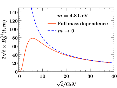
Refer to caption
Refer to caption
Figure 14: Massive b𝑏b-quark beam function (left panel) and the convolution between two of these (right panel) together with the m0𝑚0m\to 0 limit as a function of tQ𝒯similar-to𝑡𝑄𝒯\sqrt{t}\sim\sqrt{Q{\mathcal{T}}}.
Refer to caption
Refer to caption
Figure 15: Secondary massive b𝑏b-quark corrections to the u𝑢u-quark beam function for Y=0𝑌0Y=0 (left panel) and the soft function (right panel) at 𝒪(αs2CFTF)𝒪superscriptsubscript𝛼𝑠2subscript𝐶𝐹subscript𝑇𝐹\mathcal{O}(\alpha_{s}^{2}C_{F}T_{F}) for μ=mb𝜇subscript𝑚𝑏\mu=m_{b} as functions of tQ𝒯similar-to𝑡𝑄𝒯\sqrt{t}\sim\sqrt{Q{\mathcal{T}}} and 𝒯similar-to𝒯\ell\sim{\mathcal{T}}, respectively.

The mass-dependent corrections to the (beam) thrust soft function are given in eq. (4.3.3). In the limit mmuch-less-than𝑚\ell\ll m all its nondistributional terms become 𝒪(2/m2)𝒪superscript2superscript𝑚2\mathcal{O}(\ell^{2}/m^{2}) power suppressed. Combining the remaining distributional terms with the contributions arising from changing the scheme of the strong coupling from nl+1subscript𝑛𝑙1n_{l}+1 to nlsubscript𝑛𝑙n_{l} flavors yields

S(2,h)(,m,μ)43LmS(1)(,μ)=δ()Hs(2)(m,μ,ν)+𝒮c(2)(,m,μ,ν)+𝒪(2m2),superscript𝑆2𝑚𝜇43subscript𝐿𝑚superscript𝑆1𝜇𝛿superscriptsubscript𝐻𝑠2𝑚𝜇𝜈superscriptsubscript𝒮𝑐2𝑚𝜇𝜈𝒪superscript2superscript𝑚2\displaystyle S^{(2,h)}(\ell,m,\mu)-\frac{4}{3}L_{m}S^{(1)}(\ell,\mu)=\delta(\ell)\,H_{s}^{(2)}(m,\mu,\nu)+\mathcal{S}_{c}^{(2)}(\ell,m,\mu,\nu)+\mathcal{O}\Bigl{(}\frac{\ell^{2}}{m^{2}}\Bigr{)}\,, (97)

in agreement with eq. (47). The massless one-loop thrust soft function S(1)superscript𝑆1S^{(1)}, the soft mass-mode function Hs(2)superscriptsubscript𝐻𝑠2H_{s}^{(2)}, and the csoft function 𝒮c(2)superscriptsubscript𝒮𝑐2\mathcal{S}_{c}^{(2)} can be found in eqs. (129), (4.1.2), and (79), respectively. For mmuch-less-than𝑚m\ll\ell the correct massless result is recovered,

S(2,h)(,m,μ)=S(2,l)(,μ)+𝒪(m22),superscript𝑆2𝑚𝜇superscript𝑆2𝑙𝜇𝒪superscript𝑚2superscript2\displaystyle S^{(2,h)}(\ell,m,\mu)=S^{(2,l)}(\ell,\mu)+\mathcal{O}\Bigl{(}\frac{m^{2}}{\ell^{2}}\Bigr{)}\,, (98)

which was already checked in ref. Gritschacher:2013tza .

In fig. 14, we show the numerical results for the one-loop massive beam function and the convolution between two of these (which is the leading order correction from primary massive quarks for the Z𝑍Z-boson production) as a function of tQ𝒯similar-to𝑡𝑄𝒯\sqrt{t}\sim\sqrt{Q{\mathcal{T}}}. The mass effects become relevant for tmb5similar-to𝑡subscript𝑚𝑏similar-to5\sqrt{t}\sim m_{b}\sim 5 GeV (corresponding to 𝒯1less-than-or-similar-to𝒯1{\mathcal{T}}\lesssim 1 GeV for Q=mZ𝑄subscript𝑚𝑍Q=m_{Z}). The corrections to the massless limit for the convolution of two beam functions is nonnegligible also for larger values. In fig. 15, we show the result for the secondary 𝒪(αs2CFTF)𝒪superscriptsubscript𝛼𝑠2subscript𝐶𝐹subscript𝑇𝐹\mathcal{O}(\alpha_{s}^{2}C_{F}T_{F}) corrections to the beam and soft function. The corrections to the massless limit for the beam function remain sizeable even for t2mbgreater-than-or-equivalent-to𝑡2subscript𝑚𝑏\sqrt{t}\gtrsim 2m_{b}. For the soft function, the mass effects are important for 𝒯mbsimilar-to𝒯similar-tosubscript𝑚𝑏{\mathcal{T}}\sim\ell\sim m_{b} and become small for >10GeV2mb10GeVsimilar-to2subscript𝑚𝑏\ell>10\,{\rm GeV}\sim 2m_{b}. Note that the small bump in the soft function in fig. 15 originates from the correction term ΔSτΔsubscript𝑆𝜏\Delta S_{\tau} in eq. (4.3.3). The associated correction in the massless limit is fully contained in the δ()𝛿\delta(\ell) term.

5 Rapidity evolution

Here, we discuss the solutions of the rapidity RGEs in eq. (13), or equivalently eqs. (34) and (40), and in particular the rapidity evolution for the mass-dependent soft function in eq. (2.4) for qTmsimilar-tosubscript𝑞𝑇𝑚q_{T}\sim m, where the massive quark corrections give rise to a different running than for massless flavors. Our primary aim here is to highlight the different features with respect to the massless case, while leaving the practical implementation for future work.

The rapidity evolution for the mass-mode matching functions Hssubscript𝐻𝑠H_{s} and Hcsubscript𝐻𝑐H_{c} according to eq. (13) has been discussed in ref. Hoang:2015vua . The evolution for the beam thrust beam function and csoft function according to eqs. (34) and (40) is completely analogous. For example, the ν𝜈\nu-evolved soft matching function Hssubscript𝐻𝑠H_{s} is given by

Hs(m,μ,ν)subscript𝐻𝑠𝑚𝜇𝜈\displaystyle H_{s}(m,\mu,\nu) =V(m,μ,ν,ν0)Hs(m,μ,ν0),absent𝑉𝑚𝜇𝜈subscript𝜈0subscript𝐻𝑠𝑚𝜇subscript𝜈0\displaystyle=V(m,\mu,\nu,\nu_{0})\,H_{s}(m,\mu,\nu_{0})\,, (99)
V(m,μ,ν,ν0)𝑉𝑚𝜇𝜈subscript𝜈0\displaystyle V(m,\mu,\nu,\nu_{0}) =exp{[4ηΓ(nl)(μ0(m),μ)4ηΓ(nl+1)(μ0(m),μ)+γν,Hs(m,μ0(m))]lnνν0}.absentdelimited-[]4superscriptsubscript𝜂Γsubscript𝑛𝑙subscript𝜇0𝑚𝜇4superscriptsubscript𝜂Γsubscript𝑛𝑙1subscript𝜇0𝑚𝜇subscript𝛾𝜈subscript𝐻𝑠𝑚subscript𝜇0𝑚𝜈subscript𝜈0\displaystyle=\exp\biggl{\{}\Big{[}4\eta_{\Gamma}^{(n_{l})}(\mu_{0}(m),\mu)-4\eta_{\Gamma}^{(n_{l}+1)}(\mu_{0}(m),\mu)+\gamma_{\nu,H_{s}}(m,\mu_{0}(m))\Big{]}\ln\frac{\nu}{\nu_{0}}\biggr{\}}\,.

The evolution function ηΓsubscript𝜂Γ\eta_{\Gamma} is defined by

ηΓ(nf)(μ0,μ)superscriptsubscript𝜂Γsubscript𝑛𝑓subscript𝜇0𝜇\displaystyle\eta_{\Gamma}^{(n_{f})}(\mu_{0},\mu) =μ0μdμμΓcusp(nf)[αs(nf)(μ)],absentsuperscriptsubscriptsubscript𝜇0𝜇dsuperscript𝜇superscript𝜇subscriptsuperscriptΓsubscript𝑛𝑓cuspdelimited-[]superscriptsubscript𝛼𝑠subscript𝑛𝑓superscript𝜇\displaystyle=\int_{\mu_{0}}^{\mu}\frac{\textrm{d}\mu^{\prime}}{\mu^{\prime}}\,\Gamma^{(n_{f})}_{\rm{cusp}}[\alpha_{s}^{(n_{f})}(\mu^{\prime})]\,, (100)

and resums the μ𝜇\mu-dependent logarithms inside the ν𝜈\nu anomalous dimension as required by consistency with the μ𝜇\mu evolution to maintain the path independence in μ𝜇\mu-ν𝜈\nu-space Chiu:2012ir . With the canonical scale choice

μ0(m)=m,subscript𝜇0𝑚𝑚\displaystyle\mu_{0}(m)=m\,, (101)

all logarithmic terms in the boundary condition γν,Hs(m,μ0(m))subscript𝛾𝜈subscript𝐻𝑠𝑚subscript𝜇0𝑚\gamma_{\nu,H_{s}}(m,\mu_{0}(m)) are minimized.

The solution of the rapidity RGE for the soft function is substantially more involved due to its two-dimensional convolution structure on pTsubscript𝑝𝑇\vec{p}_{T}. The formal solution of the rapidity RGE for massless quarks in eq. (2.1) is most conveniently found by Fourier transforming to impact parameter space with b=|b|𝑏𝑏b=|\vec{b}|, where the rapidity RGE becomes multiplicative

νddνS~(nf)(b,μ,ν)=γ~ν,S(nf)(b,μ)S~(nf)(b,μ,ν).𝜈dd𝜈superscript~𝑆subscript𝑛𝑓𝑏𝜇𝜈subscriptsuperscript~𝛾subscript𝑛𝑓𝜈𝑆𝑏𝜇superscript~𝑆subscript𝑛𝑓𝑏𝜇𝜈\displaystyle\nu\frac{\textrm{d}}{\textrm{d}\nu}\,\tilde{S}^{(n_{f})}(b,\mu,\nu)=\tilde{\gamma}^{(n_{f})}_{\nu,S}(b,\mu)\,\tilde{S}^{(n_{f})}(b,\mu,\nu)\,. (102)

The consistency (path independence) between μ𝜇\mu and ν𝜈\nu evolution requires the rapidity anomalous dimension in Fourier space to satisfy

μddμγ~ν,S(nf)(b,μ)=4Γcusp[αs(nf)(μ)].𝜇dd𝜇subscriptsuperscript~𝛾subscript𝑛𝑓𝜈𝑆𝑏𝜇4subscriptΓcuspdelimited-[]superscriptsubscript𝛼𝑠subscript𝑛𝑓𝜇\displaystyle\mu\frac{\textrm{d}}{\textrm{d}\mu}\,\tilde{\gamma}^{(n_{f})}_{\nu,S}(b,\mu)=-4\,\Gamma_{\rm{cusp}}[\alpha_{s}^{(n_{f})}(\mu)]\,. (103)

Its solution is given by

γ~ν,S(nf)(b,μ)=4ηΓ(nf)(μ0(b),μ)+γ~ν,S(nf)(b,μ0(b)).subscriptsuperscript~𝛾subscript𝑛𝑓𝜈𝑆𝑏𝜇4superscriptsubscript𝜂Γsubscript𝑛𝑓subscript𝜇0𝑏𝜇subscriptsuperscript~𝛾subscript𝑛𝑓𝜈𝑆𝑏subscript𝜇0𝑏\displaystyle\tilde{\gamma}^{(n_{f})}_{\nu,S}(b,\mu)=-4\eta_{\Gamma}^{(n_{f})}(\mu_{0}(b),\mu)+\tilde{\gamma}^{(n_{f})}_{\nu,S}(b,\mu_{0}(b))\,. (104)

The logarithms of ln(μbeγE/2)𝜇𝑏superscript𝑒subscript𝛾𝐸2\ln(\mu\,b\,e^{\gamma_{E}}/2) in the second boundary term are eliminated by the canonical scale choice

μ0(l)(b)=2eγEb.subscriptsuperscript𝜇𝑙0𝑏2superscript𝑒subscript𝛾𝐸𝑏\displaystyle\mu^{(l)}_{0}(b)=\frac{2\,e^{-\gamma_{E}}}{b}\,. (105)

With this choice, the ν𝜈\nu evolution of the soft function in Fourier space at any given scale μ𝜇\mu is given by

S~(b,μ,ν)=S~(b,μ,ν0)exp[γ~ν,S(nf)(b,μ)lnνν0].~𝑆𝑏𝜇𝜈~𝑆𝑏𝜇subscript𝜈0subscriptsuperscript~𝛾subscript𝑛𝑓𝜈𝑆𝑏𝜇𝜈subscript𝜈0\displaystyle\tilde{S}(b,\mu,\nu)=\tilde{S}(b,\mu,\nu_{0})\exp\biggl{[}\tilde{\gamma}^{(n_{f})}_{\nu,S}(b,\mu)\,\ln\frac{\nu}{\nu_{0}}\biggr{]}\,. (106)

As is well known, the rapidity evolution kernel becomes intrinsically nonperturbative at 1/bΛQCDmuch-less-than1𝑏subscriptΛQCD1/b\ll\Lambda_{\rm QCD} Collins:1981uk ; Collins:1981va ; Collins:1984kg . This nonperturbative sensitivity appears through the resummed rapidity anomalous dimension, which with the canonical scale choice in eq. (105) gets evaluated at αs(1/b)subscript𝛼𝑠1𝑏\alpha_{s}(1/b). It is important to note that this is not an artefact of performing the evolution in Fourier space. Rather this is a physical effect, which also happens when the ν𝜈\nu evolution is consistently performed in momentum space. As shown in ref. Ebert:2016gcn , in this case the appropriate resummed result for γν,S(pT,μ)subscript𝛾𝜈𝑆subscript𝑝𝑇𝜇\gamma_{\nu,S}(\vec{p}_{T},\mu) explicitly depends on αs(pT)subscript𝛼𝑠subscript𝑝𝑇\alpha_{s}(p_{T}), which means it becomes nonperturbative for pTΛQCDless-than-or-similar-tosubscript𝑝𝑇subscriptΛQCDp_{T}\lesssim\Lambda_{\rm QCD}.

For the massive quark corrections in the regime qTmsimilar-tosubscript𝑞𝑇𝑚q_{T}\sim m the μ𝜇\mu dependence of the rapidity anomalous dimension is the same as for the massless quarks, i.e. eq. (103), such that

γ~ν,S(h)(b,m,μ)=4ηΓ(nl)(μ0(b,m),μ)4ηΓ(nl+1)(μ0(b,m),μ)+γ~ν,S(h)(b,m,μ0(b,m)).subscriptsuperscript~𝛾𝜈𝑆𝑏𝑚𝜇4superscriptsubscript𝜂Γsubscript𝑛𝑙subscript𝜇0𝑏𝑚𝜇4superscriptsubscript𝜂Γsubscript𝑛𝑙1subscript𝜇0𝑏𝑚𝜇subscriptsuperscript~𝛾𝜈𝑆𝑏𝑚subscript𝜇0𝑏𝑚\displaystyle\tilde{\gamma}^{(h)}_{\nu,S}(b,m,\mu)=4\eta_{\Gamma}^{(n_{l})}(\mu_{0}(b,m),\mu)-4\eta_{\Gamma}^{(n_{l}+1)}(\mu_{0}(b,m),\mu)+\tilde{\gamma}^{(h)}_{\nu,S}(b,m,\mu_{0}(b,m))\,. (107)

Here γ~ν,S(h)subscriptsuperscript~𝛾𝜈𝑆\tilde{\gamma}^{(h)}_{\nu,S} denotes only the contributions of the massive flavor to the full anomalous dimension. The explicit mass dependence arises in the μ𝜇\mu-independent boundary contribution, which depends on both b𝑏b and m𝑚m. From the relations in eqs. (26) and (24) we can directly infer the limiting behavior to the anomalous dimension,

γ~ν,S(b,m,μ)subscript~𝛾𝜈𝑆𝑏𝑚𝜇\displaystyle\tilde{\gamma}_{\nu,S}(b,m,\mu) =γ~ν,S(nl+1)(b,μ)+𝒪(m2b2),absentsuperscriptsubscript~𝛾𝜈𝑆subscript𝑛𝑙1𝑏𝜇𝒪superscript𝑚2superscript𝑏2\displaystyle=\tilde{\gamma}_{\nu,S}^{(n_{l}+1)}(b,\mu)+\mathcal{O}(m^{2}b^{2})\,,
γ~ν,S(b,m,μ)subscript~𝛾𝜈𝑆𝑏𝑚𝜇\displaystyle\tilde{\gamma}_{\nu,S}(b,m,\mu) =γ~ν,S(nl)(b,μ)+γν,Hs(m,μ)+𝒪(1m2b2).absentsuperscriptsubscript~𝛾𝜈𝑆subscript𝑛𝑙𝑏𝜇subscript𝛾𝜈subscript𝐻𝑠𝑚𝜇𝒪1superscript𝑚2superscript𝑏2\displaystyle=\tilde{\gamma}_{\nu,S}^{(n_{l})}(b,\mu)+\gamma_{\nu,H_{s}}(m,\mu)+\mathcal{O}\Bigl{(}\frac{1}{m^{2}b^{2}}\Bigr{)}\,. (108)

This means that the massive quark corrections γ~ν,S(h)subscriptsuperscript~𝛾𝜈𝑆\tilde{\gamma}^{(h)}_{\nu,S} are the same as for a massless flavor in the limit m1/bmuch-less-than𝑚1𝑏m\ll 1/b and are the same as the rapidity anomalous dimension of the soft mass mode function Hssubscript𝐻𝑠H_{s} in the limit 1/bmmuch-less-than1𝑏𝑚1/b\ll m, provided one uses the (nl+1)subscript𝑛𝑙1(n_{l}+1) and (nl)subscript𝑛𝑙(n_{l})-flavor scheme for αssubscript𝛼𝑠\alpha_{s}, respectively. To eliminate the logarithms inside γ~ν,S(h)subscriptsuperscript~𝛾𝜈𝑆\tilde{\gamma}^{(h)}_{\nu,S}, the canonical scale choice μ0(b,m)subscript𝜇0𝑏𝑚\mu_{0}(b,m) should behave like the massless case for m1/bmuch-less-than𝑚1𝑏m\ll 1/b and like the choice for the mass-mode matching functions for m1/bmuch-greater-than𝑚1𝑏m\gg 1/b,

μ0(h)(b,m)subscriptsuperscript𝜇0𝑏𝑚\displaystyle\mu^{(h)}_{0}(b,m) μ0(l)(b)=2eγEbsimilar-toabsentsubscriptsuperscript𝜇𝑙0𝑏2superscriptesubscript𝛾𝐸𝑏\displaystyle\sim\mu^{(l)}_{0}(b)=\frac{2\,\mathrm{e}^{-\gamma_{E}}}{b} for1/b,for1𝑏\displaystyle\text{for}\quad 1/b\to\infty\,,
μ0(h)(b,m)subscriptsuperscript𝜇0𝑏𝑚\displaystyle\mu^{(h)}_{0}(b,m) msimilar-toabsent𝑚\displaystyle\sim m for1/b0.for1𝑏0\displaystyle\text{for}\quad 1/b\to 0\,. (109)

Since μ0(h)(b,m)subscriptsuperscript𝜇0𝑏𝑚\mu^{(h)}_{0}(b,m) freezes out naturally at the perturbative mass scale for 1/b01𝑏01/b\to 0, the nonperturbative sensitivity in the ν𝜈\nu evolution gets regulated by the quark mass for the massive quark contributions.

We first illustrate this behavior in a simple one-loop toy example: We consider the radiation of a massive gluon (with mass M𝑀M) having the same couplings as a (massless) gluon in QCD, which exhibits the main features of the full results for secondary massive quarks. The associated corrections are obtained in the calculations of app. B.4.1 as intermediate results for the two-loop case. In b𝑏b-space the one-loop rapidity anomalous dimensions for massless and massive gluons are given by

γ~ν,S(1)(b,μ)superscriptsubscript~𝛾𝜈𝑆1𝑏𝜇\displaystyle\tilde{\gamma}_{\nu,S}^{(1)}(b,\mu) =CF 8Lb,absentsubscript𝐶𝐹8subscript𝐿𝑏\displaystyle=-C_{F}\,8L_{b}\,,
γ~ν,S(1)(b,M,μ)superscriptsubscript~𝛾𝜈𝑆1𝑏𝑀𝜇\displaystyle\tilde{\gamma}_{\nu,S}^{(1)}(b,M,\mu) =CF[8LM+16K0(bM)],absentsubscript𝐶𝐹delimited-[]8subscript𝐿𝑀16subscript𝐾0𝑏𝑀\displaystyle=C_{F}\,\Bigl{[}8L_{M}+16K_{0}(bM)\Bigr{]}\,, (110)

where K0subscript𝐾0K_{0} denotes the modified Bessel function of the second kind and

Lblnb2μ2e2γE4,LMlnM2μ2.formulae-sequencesubscript𝐿𝑏superscript𝑏2superscript𝜇2superscripte2subscript𝛾𝐸4subscript𝐿𝑀superscript𝑀2superscript𝜇2\displaystyle L_{b}\equiv\ln\frac{b^{2}\mu^{2}\mathrm{e}^{2\gamma_{E}}}{4}\,,\qquad L_{M}\equiv\ln\frac{M^{2}}{\mu^{2}}\,. (111)

The mass-dependent result has the limiting behavior

γ~ν,S(1)(b,M,μ)superscriptsubscript~𝛾𝜈𝑆1𝑏𝑀𝜇\displaystyle\tilde{\gamma}_{\nu,S}^{(1)}(b,M,\mu) =CF 8Lb+𝒪(M2b2),absentsubscript𝐶𝐹8subscript𝐿𝑏𝒪superscript𝑀2superscript𝑏2\displaystyle=-C_{F}\,8L_{b}+\mathcal{O}(M^{2}b^{2})\,,
γ~ν,S(1)(b,M,μ)superscriptsubscript~𝛾𝜈𝑆1𝑏𝑀𝜇\displaystyle\tilde{\gamma}_{\nu,S}^{(1)}(b,M,\mu) =CF 8LM+𝒪(1M2b2),absentsubscript𝐶𝐹8subscript𝐿𝑀𝒪1superscript𝑀2superscript𝑏2\displaystyle=C_{F}\,8L_{M}+\mathcal{O}\Bigl{(}\frac{1}{M^{2}b^{2}}\Bigr{)}\;, (112)

in close analogy to eq. (5). A natural choice to eliminate any large terms in eq. (5) in both limits is

μ0(h)(b,M)=MeK0(bM).subscriptsuperscript𝜇0𝑏𝑀𝑀superscript𝑒subscript𝐾0𝑏𝑀\displaystyle\mu^{(h)}_{0}(b,M)=M\,e^{K_{0}(bM)}\,. (113)

for which γ~ν,S(1)(b,M,μ0(h)(b,M))subscriptsuperscript~𝛾1𝜈𝑆𝑏𝑀subscriptsuperscript𝜇0𝑏𝑀\tilde{\gamma}^{(1)}_{\nu,S}(b,M,\mu^{(h)}_{0}(b,M)) just vanishes. The behavior of this choice as a function of b𝑏b compared to the massless result is shown in fig. 16.
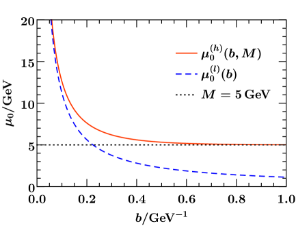
Refer to caption
Figure 16: The canonical scales μ0(h)(b,M)subscriptsuperscript𝜇0𝑏𝑀\mu^{(h)}_{0}(b,M) for the massive case (red, solid) and μ0(l)(b)=μ0(b,M=0)superscriptsubscript𝜇0𝑙𝑏subscript𝜇0𝑏𝑀0\mu_{0}^{(l)}(b)=\mu_{0}(b,M=0) for the massless case (blue, dashed) with M=5𝑀5M=5 GeV.

For the full secondary massive quark corrections at 𝒪(αs2)𝒪superscriptsubscript𝛼𝑠2\mathcal{O}(\alpha_{s}^{2}) the Fourier transform of eq. (4.3.1) reads (expanded in terms of αs(nl+1)superscriptsubscript𝛼𝑠subscript𝑛𝑙1\alpha_{s}^{(n_{l}+1)} as in eq. (49))

γ~ν,S(2,h)(b,m,μ)superscriptsubscript~𝛾𝜈𝑆2𝑏𝑚𝜇\displaystyle\tilde{\gamma}_{\nu,S}^{(2,h)}(b,m,\mu) =CF{323LbLm163Lm21609Lm44827\displaystyle=C_{F}\,\biggl{\{}-\frac{32}{3}L_{b}L_{m}-\frac{16}{3}L_{m}^{2}-\frac{160}{9}L_{m}-\frac{448}{27}
+8π3[2G1,3 3,0(320,0,0|m2b2)+G1,3 3,0(520,0,1|m2b2)]},\displaystyle\quad+\frac{8\sqrt{\pi}}{3}\Bigl{[}2\,G^{\,3,0}_{1,3}\Big{\lparen}\begin{smallmatrix}\frac{3}{2}\\ 0,0,0\end{smallmatrix}\Big{|}\,m^{2}b^{2}\Big{\rparen}+G^{\,3,0}_{1,3}\Big{\lparen}\begin{smallmatrix}\frac{5}{2}\\ 0,0,1\end{smallmatrix}\Big{|}\,m^{2}b^{2}\Big{\rparen}\Bigr{]}\biggr{\}}\,, (114)

where G𝐺G denotes a Meijer G function. This result has the limiting behavior

γ~ν,S(2,h)(b,m,μ)superscriptsubscript~𝛾𝜈𝑆2𝑏𝑚𝜇\displaystyle\tilde{\gamma}_{\nu,S}^{(2,h)}(b,m,\mu) =CF(163Lb2+1609Lb+44827)+𝒪(m2b2),absentsubscript𝐶𝐹163superscriptsubscript𝐿𝑏21609subscript𝐿𝑏44827𝒪superscript𝑚2superscript𝑏2\displaystyle=C_{F}\,\biggl{(}\frac{16}{3}L_{b}^{2}+\frac{160}{9}L_{b}+\frac{448}{27}\biggr{)}+\mathcal{O}(m^{2}b^{2})\,,
γ~ν,S(2,h)(b,m,μ)43Lmγ~ν,S(1)(b,μ)superscriptsubscript~𝛾𝜈𝑆2𝑏𝑚𝜇43subscript𝐿𝑚superscriptsubscript~𝛾𝜈𝑆1𝑏𝜇\displaystyle\tilde{\gamma}_{\nu,S}^{(2,h)}(b,m,\mu)-\frac{4}{3}L_{m}\tilde{\gamma}_{\nu,S}^{(1)}(b,\mu) =CF(163Lm21609Lm44827)+𝒪(1m2b2).absentsubscript𝐶𝐹163superscriptsubscript𝐿𝑚21609subscript𝐿𝑚44827𝒪1superscript𝑚2superscript𝑏2\displaystyle=C_{F}\,\biggl{(}-\frac{16}{3}L_{m}^{2}-\frac{160}{9}L_{m}-\frac{448}{27}\biggr{)}+\mathcal{O}\Bigl{(}\frac{1}{m^{2}b^{2}}\Bigr{)}\,. (115)

Hence, the correct massless limit is recovered, while in the large-mass limit one obtains the anomalous dimension in eq. (4.1.2). Note that one needs to perform a change for the strong coupling between the nl+1subscript𝑛𝑙1n_{l}+1 and nlsubscript𝑛𝑙n_{l} flavor schemes to obtain both limits correctly. To minimize the logarithms for any regime one should thus adopt a canonical scale choice that satisfies eq. (5), as for example in eq. (113).

6 Outlook: Phenomenological impact for Drell-Yan

Our results can be applied to properly take into account bottom quark mass effects for the Drell-Yan qTsubscript𝑞𝑇q_{T} spectrum at NNLL. While a full resummation analysis is beyond the scope of this paper, we can estimate the potential size of the quark-mass effects by looking at the fixed-order qTsubscript𝑞𝑇q_{T} spectrum.

In fig. 17, we show separately the contributions from primary and secondary massive quarks to the cross section at 𝒪(αs2)𝒪superscriptsubscript𝛼𝑠2\mathcal{O}(\alpha_{s}^{2}), normalized to the 𝒪(αs)𝒪subscript𝛼𝑠\mathcal{O}(\alpha_{s}) spectrum dσ(1)dsuperscript𝜎1\textrm{d}\sigma^{(1)} including all flavors (treating the charm as a massless flavor). We utilize the MMHT2014 NNLO PDFs Harland-Lang:2014zoa and evaluate the contributions for μ=mb=4.8𝜇subscript𝑚𝑏4.8\mu=m_{b}=4.8 GeV, Q=mZ𝑄subscript𝑚𝑍Q=m_{Z}, Y=0𝑌0Y=0, and Ecm=13subscript𝐸cm13E_{\rm cm}=13 TeV. Note that the secondary mass contributions at 𝒪(αs2)𝒪superscriptsubscript𝛼𝑠2\mathcal{O}(\alpha_{s}^{2}) are explicitly μ𝜇\mu-dependent and scheme-dependent, the nonsingular mass correction, i.e. the difference between the full massive result for μmbsimilar-to𝜇subscript𝑚𝑏\mu\sim m_{b} and the massless limit (encoded partially in a massive PDF), is μ𝜇\mu independent at this order. As can be seen, the relative contribution of the bb¯𝑏¯𝑏b\bar{b}-initiated channel grows with larger qTsubscript𝑞𝑇q_{T}, while the impact of the secondary contributions including the full mass dependence is at the sub-percent level throughout the spectrum. As expected, the nonsingular mass corrections are very small for mbqTmuch-less-thansubscript𝑚𝑏subscript𝑞𝑇m_{b}\ll q_{T}, but can reach the order of percent for qTmbsimilar-tosubscript𝑞𝑇subscript𝑚𝑏q_{T}\sim m_{b}, which roughly corresponds to the peak region of the distribution where the cross section is largest.

The same can also be seen in fig. 18, where we show the mass nonsingular corrections to the massless limit for primary and secondary contributions as well as their sum. They are shown for μ=mb𝜇subscript𝑚𝑏\mu=m_{b} on the left and for μ=qT𝜇subscript𝑞𝑇\mu=q_{T} on the right. We see that these corrections are (at fixed order) indeed only weakly dependent on the value of μ𝜇\mu (for qT2greater-than-or-equivalent-tosubscript𝑞𝑇2q_{T}\gtrsim 2 GeV). All in all, the bottom quark mass can have a relevant effect for high precision predictions of the qTsubscript𝑞𝑇q_{T}-spectrum at the order of percent around the peak of the distribution (5similar-toabsent5\sim 5 GeV). Below the peak of the distribution the fixed-order result is of course not expected to give a reliable quantitative result, and furthermore nonperturbative corrections become important in this regime. Nevertheless, we expect the qualitative features like the sign and order of magnitude of the mass effects to provide an indication for the behaviour of the full resummed result.

For W𝑊W production sizable corrections from bottom quark effects arise only through secondary contributions (due to the strong CKM suppression of the primary contributions), which have a similar impact as for Z𝑍Z-production. On the other hand, charm-initiated production plays an important role and enters already at 𝒪(αs)𝒪subscript𝛼𝑠\mathcal{O}(\alpha_{s}). Estimating the nonsingular mass corrections for qTmcsimilar-tosubscript𝑞𝑇subscript𝑚𝑐q_{T}\sim m_{c} is more subtle, since higher-order corrections in the strong coupling and nonperturbative effects are likely to dominate the effect from the known beam function at 𝒪(αs)𝒪subscript𝛼𝑠\mathcal{O}(\alpha_{s}) at these low scales. Thus, we do not attempt to determine their characteristic size here and leave this to future work. An analysis based on the leading-order matrix element and its potential impact on the determination of mWsubscript𝑚𝑊m_{W} can be found in ref. Berge:2005rv .
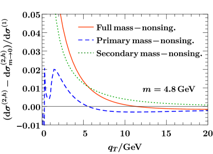
Refer to caption
Refer to caption
Figure 17: Primary (left panel) and secondary (right panel) massive bottom quark contributions for the Z𝑍Z-boson qTsubscript𝑞𝑇q_{T} spectrum at fixed 𝒪(αs2TF2)𝒪superscriptsubscript𝛼𝑠2superscriptsubscript𝑇𝐹2\mathcal{O}(\alpha_{s}^{2}T_{F}^{2}) and 𝒪(αs2CFTF)𝒪superscriptsubscript𝛼𝑠2subscript𝐶𝐹subscript𝑇𝐹\mathcal{O}(\alpha_{s}^{2}C_{F}T_{F}), respectively. The results are given relative to the full 𝒪(αs)𝒪subscript𝛼𝑠\mathcal{O}(\alpha_{s}) result including all flavors.
Refer to caption
Refer to caption
Figure 18: Different types of mass nonsingular corrections for Z𝑍Z-boson production at μ=mb𝜇subscript𝑚𝑏\mu=m_{b} (left panel) and μ=qT𝜇subscript𝑞𝑇\mu=q_{T} (right panel).

7 Conclusions

Massive quark effects provide a challenge for high-precision predictions at colliders. Using a SCET-based factorization framework, we have discussed how to systematically incorporate massive quark corrections into exclusive differential cross sections at the LHC, using the measurement of the transverse momentum qTsubscript𝑞𝑇q_{T} and beam thrust for Drell-Yan production as prototypical examples. We have discussed the relevant factorization setup for the different hierarchies between the mass scale and the other relevant kinematic scales. We find that the presence of (secondary) massive quarks can lead to the emergence or alteration of rapidity logarithms thus changing the resummation structure in a nontrivial way.

The generic framework for the description of mass effects generalizes to other exclusive cross sections with different jet-resolution measurements and final-state kinematic cuts, which will require additional calculations of the relevant factorization ingredients. Our results for the beam thrust spectrum allow for a systematic inclusion of massive quark effects into the Geneva Monte-Carlo program Alioli:2012fc ; Alioli:2015toa at NNLL+{}^{\prime}+NNLO in its underlying jet resolution variable. Several of our results are also immediately relevant for other processes besides Drell-Yan. The massive quark beam functions are relevant for any heavy-quark initiated process, for example exclusive bb¯H𝑏¯𝑏𝐻b\bar{b}H-production. The mass-dependent soft function and rapidity anomalous dimension at 𝒪(αs2)𝒪superscriptsubscript𝛼𝑠2\mathcal{O}(\alpha_{s}^{2}) satisfy Casimir scaling and can be therefore also utilized for the description of gluon-fusion processes, e.g. the Higgs qTsubscript𝑞𝑇q_{T}-spectrum.

An important application of our framework is to the precise theoretical description of the Drell-Yan qTsubscript𝑞𝑇q_{T} spectrum. To this end, we have computed all required mass-dependent beam and soft functions up to 𝒪(αs2)𝒪superscriptsubscript𝛼𝑠2\mathcal{O}(\alpha_{s}^{2}) allowing for the description of massive quark effects in the Drell-Yan qTsubscript𝑞𝑇q_{T} spectrum at NNLL. In particular, our results provide an important ingredient for a detailed investigation of quark-mass effects in the ratio of W𝑊W and Z𝑍Z boson spectra at small qTsubscript𝑞𝑇q_{T}, which is important for the precision measurement of the W𝑊W-boson mass at the LHC.

Acknowledgements.
We thank Markus Ebert and Maximilian Stahlhofen for useful discussions. This work was supported by the German Science Foundation (DFG) through the Emmy-Noether Grant No. TA 867/1-1 and the Collaborative Research Center (SFB) 676 Particles, Strings and the Early Universe. D.S. is supported by the Austrian Science Fund (FWF) under the Doctoral Program No. W1252-N27 Particles and Interactions. We also thank the Erwin-Schrödinger Institute (ESI) for partial support in the framework of the ESI program Challenges and Concepts for Field Theory and Applications in the Era of LHC Run-2.

Appendix A Results for massless quarks

Here we summarize the relevant results with massless quarks for the hard, beam, and soft functions.

A.1 Hard function

The massless quark hard function is directly related to the QCD form factor and has been computed at 𝒪(αs2)𝒪superscriptsubscript𝛼𝑠2\mathcal{O}(\alpha_{s}^{2}) in ref. Matsuura . The 𝒪(αs)𝒪subscript𝛼𝑠\mathcal{O}(\alpha_{s}) and 𝒪(αs2CFTF)𝒪superscriptsubscript𝛼𝑠2subscript𝐶𝐹subscript𝑇𝐹\mathcal{O}(\alpha_{s}^{2}C_{F}T_{F}) corrections read in an expansion in terms of αs=αs(nf)(μ)subscript𝛼𝑠superscriptsubscript𝛼𝑠subscript𝑛𝑓𝜇\alpha_{s}=\alpha_{s}^{(n_{f})}(\mu) in analogy to eq. (49) (with LQ=ln(Q2/μ2)subscript𝐿𝑄superscript𝑄2superscript𝜇2L_{Q}=\ln(Q^{2}/\mu^{2}))

H(1)(Q,μ)superscript𝐻1𝑄𝜇\displaystyle H^{(1)}(Q,\mu) =H(0)(Q)CF(2LQ2+6LQ16+7π23),absentsuperscript𝐻0𝑄subscript𝐶𝐹2superscriptsubscript𝐿𝑄26subscript𝐿𝑄167superscript𝜋23\displaystyle=H^{(0)}(Q)\,C_{F}\,\Bigl{(}-2L_{Q}^{2}+6L_{Q}-16+\frac{7\pi^{2}}{3}\Bigr{)}\,, (116)
H(2,l)(Q,μ)superscript𝐻2𝑙𝑄𝜇\displaystyle H^{(2,l)}(Q,\mu) =H(0)(Q)CF[89LQ3+769LQ2(8362716π29)LQ+408581182π227+8ζ39],absentsuperscript𝐻0𝑄subscript𝐶𝐹delimited-[]89superscriptsubscript𝐿𝑄3769superscriptsubscript𝐿𝑄28362716superscript𝜋29subscript𝐿𝑄408581182superscript𝜋2278subscript𝜁39\displaystyle=H^{(0)}(Q)\,C_{F}\,\biggl{[}-\frac{8}{9}L_{Q}^{3}+\frac{76}{9}L_{Q}^{2}-\Bigl{(}\frac{836}{27}-\frac{16\pi^{2}}{9}\Bigr{)}L_{Q}+\frac{4085}{81}-\frac{182\pi^{2}}{27}+\frac{8\zeta_{3}}{9}\biggr{]}\,,

where H(0)superscript𝐻0H^{(0)} is the tree-level contribution. Note that for a single quark flavor there is in addition a nonvanishing correction to the axial current contribution relevant for Z𝑍Z-boson production, but cancels within an isospin doublet for massless quarks.

The anomalous dimensions are

γH(1)(Q,μ)superscriptsubscript𝛾𝐻1𝑄𝜇\displaystyle\gamma_{H}^{(1)}(Q,\mu) =CF(8LQ12),absentsubscript𝐶𝐹8subscript𝐿𝑄12\displaystyle=C_{F}\,(8L_{Q}-12)\,,
γH(2,l)(Q,μ)superscriptsubscript𝛾𝐻2𝑙𝑄𝜇\displaystyle\gamma_{H}^{(2,l)}(Q,\mu) =CF(1609LQ+52027+8π23).absentsubscript𝐶𝐹1609subscript𝐿𝑄520278superscript𝜋23\displaystyle=C_{F}\,\biggl{(}-\frac{160}{9}L_{Q}+\frac{520}{27}+\frac{8\pi^{2}}{3}\biggr{)}\,. (117)

A.2 Beam functions

A.2.1 TMD beam function

The matching coefficients entering the TMD beam function have been computed at 𝒪(αs2)𝒪superscriptsubscript𝛼𝑠2\mathcal{O}(\alpha_{s}^{2}) in various schemes Catani:2012qa ; Gehrmann:2012ze ; Gehrmann:2014yya ; Echevarria:2016scs and are obtained for the symmetric η𝜂\eta-regulator in ref. Luebbert:2016itl . The results at 𝒪(αs)𝒪subscript𝛼𝑠\mathcal{O}(\alpha_{s}) are

qg(1)(pT,z,μ)superscriptsubscript𝑞𝑔1subscript𝑝𝑇𝑧𝜇\displaystyle\mathcal{I}_{qg}^{(1)}(\vec{p}_{T},z,\mu) =θ(z)θ(1z)TF[2Pqg(z)0(pT,μ)+4z(1z)δ(2)(pT)],absent𝜃𝑧𝜃1𝑧subscript𝑇𝐹delimited-[]2subscript𝑃𝑞𝑔𝑧subscript0subscript𝑝𝑇𝜇4𝑧1𝑧superscript𝛿2subscript𝑝𝑇\displaystyle=\theta(z)\theta(1-z)\,T_{F}\,\Bigl{[}2P_{qg}(z)\mathcal{L}_{0}(\vec{p}_{T},\mu)+4z(1-z)\delta^{(2)}(\vec{p}_{T})\Bigr{]}\,, (118)
qq(1)(pT,z,μ,νω)superscriptsubscript𝑞𝑞1subscript𝑝𝑇𝑧𝜇𝜈𝜔\displaystyle\mathcal{I}_{qq}^{(1)}\Bigl{(}\vec{p}_{T},z,\mu,\frac{\nu}{\omega}\Bigr{)} =θ(z)CF{0(pT,μ)[(4lnνω+3)δ(1z)+2Pqq(z)]\displaystyle=\theta(z)\,C_{F}\,\Bigl{\{}\mathcal{L}_{0}(\vec{p}_{T},\mu)\Bigl{[}-\Bigl{(}4\ln\frac{\nu}{\omega}+3\Bigr{)}\delta(1-z)+2P_{qq}(z)\Bigr{]}
+2δ(2)(pT)θ(1z)(1z)}.\displaystyle\quad+2\delta^{(2)}(\vec{p}_{T})\,\theta(1-z)(1-z)\Bigr{\}}\,. (119)

The splitting functions are

Pqg(z)=z2+(1z)2,Pqq(z)=20(1z)+32δ(1z)θ(1z)(1+z).formulae-sequencesubscript𝑃𝑞𝑔𝑧superscript𝑧2superscript1𝑧2subscript𝑃𝑞𝑞𝑧2subscript01𝑧32𝛿1𝑧𝜃1𝑧1𝑧\displaystyle P_{qg}(z)=z^{2}+(1-z)^{2}\,,\qquad P_{qq}(z)=2\mathcal{L}_{0}(1-z)+\frac{3}{2}\delta(1-z)-\theta(1-z)(1+z)\,. (120)

At 𝒪(αs2CFTF)𝒪superscriptsubscript𝛼𝑠2subscript𝐶𝐹subscript𝑇𝐹\mathcal{O}(\alpha_{s}^{2}C_{F}T_{F}) the massless matching coefficient is given by

qq(2,l)(pT,z,μ,νω)superscriptsubscript𝑞𝑞2𝑙subscript𝑝𝑇𝑧𝜇𝜈𝜔\displaystyle\mathcal{I}_{qq}^{(2,l)}\Bigl{(}\vec{p}_{T},z,\mu,\frac{\nu}{\omega}\Bigr{)} =θ(z)CF{1(pT,μ)[1630(1z)163lnνωδ(1z)83θ(1z)(1+z)]\displaystyle=\theta(z)\,C_{F}\biggl{\{}\mathcal{L}_{1}(\vec{p}_{T},\mu)\biggl{[}\frac{16}{3}\mathcal{L}_{0}(1-z)-\frac{16}{3}\ln\frac{\nu}{\omega}\,\delta(1-z)-\frac{8}{3}\theta(1-z)(1+z)\biggr{]}
+0(pT,μ)[8090(1z)+809lnνωδ(1z)\displaystyle\quad+\mathcal{L}_{0}(\vec{p}_{T},\mu)\biggl{[}-\frac{80}{9}\mathcal{L}_{0}(1-z)+\frac{80}{9}\ln\frac{\nu}{\omega}\,\delta(1-z)
+θ(1z)(831+z21zlnz+169+64z9)]\displaystyle\qquad+\theta(1-z)\biggl{(}-\frac{8}{3}\frac{1+z^{2}}{1-z}\ln z+\frac{16}{9}+\frac{64z}{9}\biggr{)}\biggr{]}
+δ(2)(pT)[224270(1z)22427lnνωδ(1z)\displaystyle\quad+\delta^{(2)}(\vec{p}_{T})\biggl{[}\frac{224}{27}\mathcal{L}_{0}(1-z)-\frac{224}{27}\ln\frac{\nu}{\omega}\,\delta(1-z)
+θ(1z)(231+z21zln2z+2091+z21zlnz1482776z27)]}.\displaystyle\qquad+\theta(1-z)\biggl{(}\frac{2}{3}\frac{1+z^{2}}{1-z}\ln^{2}z+\frac{20}{9}\frac{1+z^{2}}{1-z}\ln z-\frac{148}{27}-\frac{76z}{27}\biggr{)}\biggr{]}\biggr{\}}\,. (121)

The anomalous dimensions of the massless quark TMD beam function, as defined in eq. (2.1), are given at 𝒪(αs)𝒪subscript𝛼𝑠\mathcal{O}(\alpha_{s}) and 𝒪(αs2CFTF)𝒪superscriptsubscript𝛼𝑠2subscript𝐶𝐹subscript𝑇𝐹\mathcal{O}(\alpha_{s}^{2}C_{F}T_{F}) by

γB(1)(νω)superscriptsubscript𝛾𝐵1𝜈𝜔\displaystyle\gamma_{B}^{(1)}\Bigl{(}\frac{\nu}{\omega}\Bigr{)} =CF(8lnνω+6),absentsubscript𝐶𝐹8𝜈𝜔6\displaystyle=C_{F}\,\Bigl{(}8\ln\frac{\nu}{\omega}+6\Bigr{)}\,,
γB(2,l)(νω)superscriptsubscript𝛾𝐵2𝑙𝜈𝜔\displaystyle\gamma_{B}^{(2,l)}\Bigl{(}\frac{\nu}{\omega}\Bigr{)} =CF(1609lnνω4316π29),absentsubscript𝐶𝐹1609𝜈𝜔4316superscript𝜋29\displaystyle=C_{F}\,\Bigl{(}-\frac{160}{9}\ln\frac{\nu}{\omega}-\frac{4}{3}-\frac{16\pi^{2}}{9}\Bigr{)}\,,
γν,B(1)(pT,μ)superscriptsubscript𝛾𝜈𝐵1subscript𝑝𝑇𝜇\displaystyle\gamma_{\nu,B}^{(1)}(\vec{p}_{T},\mu) =CF 40(pT,μ),absentsubscript𝐶𝐹4subscript0subscript𝑝𝑇𝜇\displaystyle=-C_{F}\,4\mathcal{L}_{0}(\vec{p}_{T},\mu)\,,
γν,B(2,l)(pT,μ)superscriptsubscript𝛾𝜈𝐵2𝑙subscript𝑝𝑇𝜇\displaystyle\gamma_{\nu,B}^{(2,l)}(\vec{p}_{T},\mu) =CF[1631(pT,μ)+8090(pT,μ)22427δ(2)(pT)].absentsubscript𝐶𝐹delimited-[]163subscript1subscript𝑝𝑇𝜇809subscript0subscript𝑝𝑇𝜇22427superscript𝛿2subscript𝑝𝑇\displaystyle=C_{F}\,\biggl{[}-\frac{16}{3}\mathcal{L}_{1}(\vec{p}_{T},\mu)+\frac{80}{9}\mathcal{L}_{0}(\vec{p}_{T},\mu)-\frac{224}{27}\delta^{(2)}(\vec{p}_{T})\biggr{]}\,. (122)

A.2.2 Virtuality-dependent beam function

The virtuality-dependent beam functions for massless quarks are known to two loop order Gaunt:2014xga ; Gaunt:2014cfa . The matching coefficients at 𝒪(αs)𝒪subscript𝛼𝑠\mathcal{O}(\alpha_{s}) read

qg(1)(t,z,μ)superscriptsubscript𝑞𝑔1𝑡𝑧𝜇\displaystyle\mathcal{I}_{qg}^{(1)}(t,z,\mu) =θ(z)θ(1z)TF{2Pqg(z)1μ20(tμ2)+δ(t)[2Pqg(z)ln1zz+4z(1z)]},absent𝜃𝑧𝜃1𝑧subscript𝑇𝐹2subscript𝑃𝑞𝑔𝑧1superscript𝜇2subscript0𝑡superscript𝜇2𝛿𝑡delimited-[]2subscript𝑃𝑞𝑔𝑧1𝑧𝑧4𝑧1𝑧\displaystyle=\theta(z)\theta(1-z)\,T_{F}\,\biggl{\{}2P_{qg}(z)\frac{1}{\mu^{2}}\mathcal{L}_{0}\Bigl{(}\frac{t}{\mu^{2}}\Bigr{)}+\delta(t)\Bigl{[}2P_{qg}(z)\ln\frac{1-z}{z}+4z(1-z)\Bigr{]}\biggr{\}}\,,
qq(1)(t,z,μ)superscriptsubscript𝑞𝑞1𝑡𝑧𝜇\displaystyle\mathcal{I}_{qq}^{(1)}(t,z,\mu) =θ(z)CF{4μ21(tμ2)δ(1z)+1μ20(tμ2)[2Pqq(z)3δ(1z)]\displaystyle=\theta(z)\,C_{F}\,\biggl{\{}\frac{4}{\mu^{2}}\mathcal{L}_{1}\Bigl{(}\frac{t}{\mu^{2}}\Bigr{)}\delta(1-z)+\frac{1}{\mu^{2}}\mathcal{L}_{0}\Bigl{(}\frac{t}{\mu^{2}}\Bigr{)}\Bigl{[}2P_{qq}(z)-3\delta(1-z)\Bigr{]}
+δ(t)[41(1z)π23δ(1z)\displaystyle\quad+\delta(t)\biggl{[}4\mathcal{L}_{1}(1-z)-\frac{\pi^{2}}{3}\delta(1-z)
+θ(1z)[2(1z2(1+z)ln(1z)21+z21zlnz]]}.\displaystyle\qquad+\theta(1-z)\Bigl{[}2(1-z-2(1+z)\ln(1-z)-2\frac{1+z^{2}}{1-z}\ln z\Bigr{]}\biggr{]}\biggr{\}}\,. (123)

The massless matching coefficient at order 𝒪(αs2CFTF)𝒪superscriptsubscript𝛼𝑠2subscript𝐶𝐹subscript𝑇𝐹\mathcal{O}(\alpha_{s}^{2}C_{F}T_{F}) for one quark flavor reads

qq(2,l)(t,z,μ)superscriptsubscript𝑞𝑞2𝑙𝑡𝑧𝜇\displaystyle\mathcal{I}_{qq}^{(2,l)}(t,z,\mu) (124)
=θ(z)CF{831μ22(tμ2)δ(1z)\displaystyle=\theta(z)\,C_{F}\biggl{\{}\frac{8}{3}\frac{1}{\mu^{2}}\mathcal{L}_{2}\Bigl{(}\frac{t}{\mu^{2}}\Bigr{)}\,\delta(1-z)
+1μ21(tμ2)[1630(1z)809δ(1z)83θ(1z)(1+z)]1superscript𝜇2subscript1𝑡superscript𝜇2delimited-[]163subscript01𝑧809𝛿1𝑧83𝜃1𝑧1𝑧\displaystyle\quad+\frac{1}{\mu^{2}}\mathcal{L}_{1}\Bigl{(}\frac{t}{\mu^{2}}\Bigr{)}\biggl{[}\frac{16}{3}\mathcal{L}_{0}(1-z)-\frac{80}{9}\delta(1-z)-\frac{8}{3}\theta(1-z)(1+z)\biggr{]}
+1μ20(tμ2)[1631(1z)8090(1z)+δ(1z)(224278π29)\displaystyle\quad+\frac{1}{\mu^{2}}\mathcal{L}_{0}\Bigl{(}\frac{t}{\mu^{2}}\Bigr{)}\biggl{[}\frac{16}{3}\mathcal{L}_{1}(1-z)-\frac{80}{9}\mathcal{L}_{0}(1-z)+\delta(1-z)\Bigl{(}\frac{224}{27}-\frac{8\pi^{2}}{9}\Bigr{)}
+θ(1z)(83(1+z)ln(1z)16(1+z2)3(1z)lnz+169+64z9)]\displaystyle\qquad+\theta(1-z)\biggl{(}-\frac{8}{3}(1+z)\ln(1-z)-\frac{16(1+z^{2})}{3(1-z)}\ln z+\frac{16}{9}+\frac{64z}{9}\biggr{)}\biggr{]}
+δ(t)[832(1z)8091(1z)+0(1z)(224278π29)\displaystyle\quad+\delta(t)\biggl{[}\frac{8}{3}\mathcal{L}_{2}(1-z)-\frac{80}{9}\mathcal{L}_{1}(1-z)+\mathcal{L}_{0}(1-z)\Bigl{(}\frac{224}{27}-\frac{8\pi^{2}}{9}\Bigr{)}
+δ(1z)(65681+10π29+40ζ39)+θ(1z)(8(1+z2)3(1z)Li2(1z)\displaystyle\qquad+\delta(1-z)\Bigl{(}-\frac{656}{81}+\frac{10\pi^{2}}{9}+\frac{40\zeta_{3}}{9}\Bigr{)}+\theta(1-z)\biggl{(}-\frac{8(1+z^{2})}{3(1-z)}\,\mathrm{Li}_{2}(1-z)
43(1+z)ln2(1z)16(1+z2)3(1z)ln(1z)lnz+10(1+z2)3(1z)ln2z431𝑧superscript21𝑧161superscript𝑧231𝑧1𝑧𝑧101superscript𝑧231𝑧superscript2𝑧\displaystyle\qquad-\frac{4}{3}(1+z)\ln^{2}(1-z)-\frac{16(1+z^{2})}{3(1-z)}\ln(1-z)\ln z+\frac{10\left(1+z^{2}\right)}{3(1-z)}\ln^{2}z
+(169+64z9)ln(1z)+4(52z+7z2)3(1z)lnz1482776z27+4π29(1+z))]}.\displaystyle\qquad+\Bigl{(}\frac{16}{9}+\frac{64z}{9}\Bigr{)}\ln(1-z)+\frac{4(5-2z+7z^{2})}{3(1-z)}\ln z-\frac{148}{27}-\frac{76z}{27}+\frac{4\pi^{2}}{9}(1+z)\biggr{)}\biggr{]}\biggr{\}}\,.

The anomalous dimension of the massless quark beam function at order 𝒪(αs)𝒪subscript𝛼𝑠\mathcal{O}(\alpha_{s}) and 𝒪(αs2CFTF)𝒪superscriptsubscript𝛼𝑠2subscript𝐶𝐹subscript𝑇𝐹\mathcal{O}(\alpha_{s}^{2}C_{F}T_{F}) are given by

γB(1)(t,μ)superscriptsubscript𝛾𝐵1𝑡𝜇\displaystyle\gamma_{B}^{(1)}(t,\mu) =CF[8μ20(tμ2)+6δ(t)],absentsubscript𝐶𝐹delimited-[]8superscript𝜇2subscript0𝑡superscript𝜇26𝛿𝑡\displaystyle=C_{F}\biggl{[}-\frac{8}{\mu^{2}}\mathcal{L}_{0}\Bigl{(}\frac{t}{\mu^{2}}\Bigr{)}+6\delta(t)\biggr{]}\,,
γB(2,l)(t,μ)superscriptsubscript𝛾𝐵2𝑙𝑡𝜇\displaystyle\gamma_{B}^{(2,l)}(t,\mu) =CF[16091μ20(tμ2)+δ(t)(484278π29)].absentsubscript𝐶𝐹delimited-[]16091superscript𝜇2subscript0𝑡superscript𝜇2𝛿𝑡484278superscript𝜋29\displaystyle=C_{F}\,\biggl{[}\frac{160}{9}\frac{1}{\mu^{2}}\mathcal{L}_{0}\Bigl{(}\frac{t}{\mu^{2}}\Bigr{)}+\delta(t)\Bigl{(}-\frac{484}{27}-\frac{8\pi^{2}}{9}\Bigr{)}\biggr{]}\,. (125)

A.3 Soft functions

A.3.1 TMD soft function

The TMD soft function for massless quarks with the symmetric η𝜂\eta-regulator has been computed at two loops in ref. Luebbert:2016itl . At 𝒪(αs)𝒪subscript𝛼𝑠\mathcal{O}(\alpha_{s}) and 𝒪(αs2CFTF)𝒪superscriptsubscript𝛼𝑠2subscript𝐶𝐹subscript𝑇𝐹\mathcal{O}(\alpha_{s}^{2}C_{F}T_{F}) it is given by

S(1)(pT,μ,ν)superscript𝑆1subscript𝑝𝑇𝜇𝜈\displaystyle S^{(1)}(\vec{p}_{T},\mu,\nu) =CF[41(pT,μ)+8lnνμ0(pT,μ)π23δ(2)(pT)],absentsubscript𝐶𝐹delimited-[]4subscript1subscript𝑝𝑇𝜇8𝜈𝜇subscript0subscript𝑝𝑇𝜇superscript𝜋23superscript𝛿2subscript𝑝𝑇\displaystyle=C_{F}\,\biggl{[}-4\mathcal{L}_{1}(\vec{p}_{T},\mu)+8\ln\frac{\nu}{\mu}\,\mathcal{L}_{0}(\vec{p}_{T},\mu)-\frac{\pi^{2}}{3}\delta^{(2)}(\vec{p}_{T})\biggr{]}\,, (126)
S(2,l)(pT,μ,ν)superscript𝑆2𝑙subscript𝑝𝑇𝜇𝜈\displaystyle S^{(2,l)}(\vec{p}_{T},\mu,\nu) =CF[1632(pT,μ)+1(pT,μ)(323lnνμ+809)0(pT,μ)(1609lnνμ+8π29)\displaystyle=C_{F}\,\biggl{[}-\frac{16}{3}\mathcal{L}_{2}(\vec{p}_{T},\mu)+\mathcal{L}_{1}(\vec{p}_{T},\mu)\Bigl{(}\frac{32}{3}\ln\frac{\nu}{\mu}+\frac{80}{9}\Bigr{)}-\mathcal{L}_{0}(\vec{p}_{T},\mu)\Bigl{(}\frac{160}{9}\ln\frac{\nu}{\mu}+\frac{8\pi^{2}}{9}\Bigr{)}
+δ(2)(pT)(44827lnνμ65681+10π298ζ39)].\displaystyle\quad+\delta^{(2)}(\vec{p}_{T})\Bigl{(}\frac{448}{27}\ln\frac{\nu}{\mu}-\frac{656}{81}+\frac{10\pi^{2}}{9}-\frac{8\zeta_{3}}{9}\Bigr{)}\biggr{]}\,. (127)

The corresponding anomalous dimensions are

γS(1)(μ,ν)subscriptsuperscript𝛾1𝑆𝜇𝜈\displaystyle\gamma^{(1)}_{S}(\mu,\nu) =CF 16lnνμ,absentsubscript𝐶𝐹16𝜈𝜇\displaystyle=-C_{F}\,16\ln\frac{\nu}{\mu}\,,
γS(2,l)(μ,ν)superscriptsubscript𝛾𝑆2𝑙𝜇𝜈\displaystyle\gamma_{S}^{(2,l)}(\mu,\nu) =CF(3209lnνμ44827+8π29),absentsubscript𝐶𝐹3209𝜈𝜇448278superscript𝜋29\displaystyle=C_{F}\,\biggl{(}\frac{320}{9}\ln\frac{\nu}{\mu}-\frac{448}{27}+\frac{8\pi^{2}}{9}\biggr{)}\,,
γν,S(1)(pT,μ)subscriptsuperscript𝛾1𝜈𝑆subscript𝑝𝑇𝜇\displaystyle\gamma^{(1)}_{\nu,S}(\vec{p}_{T},\mu) =CF 80(pT,μ),absentsubscript𝐶𝐹8subscript0subscript𝑝𝑇𝜇\displaystyle=C_{F}\,8\mathcal{L}_{0}(\vec{p}_{T},\mu)\,,
γν,S(2,l)(pT,μ)superscriptsubscript𝛾𝜈𝑆2𝑙subscript𝑝𝑇𝜇\displaystyle\gamma_{\nu,S}^{(2,l)}(\vec{p}_{T},\mu) =CF[3231(pT,μ)16090(pT,μ)+44827δ(2)(pT)].absentsubscript𝐶𝐹delimited-[]323subscript1subscript𝑝𝑇𝜇1609subscript0subscript𝑝𝑇𝜇44827superscript𝛿2subscript𝑝𝑇\displaystyle=C_{F}\,\biggl{[}\frac{32}{3}\mathcal{L}_{1}(\vec{p}_{T},\mu)-\frac{160}{9}\mathcal{L}_{0}(\vec{p}_{T},\mu)+\frac{448}{27}\delta^{(2)}(\vec{p}_{T})\biggr{]}\,. (128)

A.3.2 Thrust soft function

The thrust soft function is known to two loops Kelley:2011ng ; Monni:2011gb . At 𝒪(αs)𝒪subscript𝛼𝑠\mathcal{O}(\alpha_{s}) and 𝒪(αs2CFTF)𝒪superscriptsubscript𝛼𝑠2subscript𝐶𝐹subscript𝑇𝐹\mathcal{O}(\alpha_{s}^{2}C_{F}T_{F}) it is given by

S(1)(,μ)superscript𝑆1𝜇\displaystyle S^{(1)}(\ell,\mu) =CF[161μ1(μ)+π23δ()],absentsubscript𝐶𝐹delimited-[]161𝜇subscript1𝜇superscript𝜋23𝛿\displaystyle=C_{F}\,\biggl{[}-16\frac{1}{\mu}\mathcal{L}_{1}\Bigl{(}\frac{\ell}{\mu}\Bigr{)}+\frac{\pi^{2}}{3}\delta(\ell)\biggr{]}\,, (129)
S(2,l)(,μ)superscript𝑆2𝑙𝜇\displaystyle S^{(2,l)}(\ell,\mu) =CF[6431μ2(μ)+32091μ1(μ)+1μ0(μ)(44827+16π29)\displaystyle=C_{F}\,\biggl{[}-\frac{64}{3}\frac{1}{\mu}\mathcal{L}_{2}\Bigl{(}\frac{\ell}{\mu}\Bigr{)}+\frac{320}{9}\frac{1}{\mu}\mathcal{L}_{1}\Bigl{(}\frac{\ell}{\mu}\Bigr{)}+\frac{1}{\mu}\mathcal{L}_{0}\Bigl{(}\frac{\ell}{\mu}\Bigr{)}\Bigl{(}-\frac{448}{27}+\frac{16\pi^{2}}{9}\Bigr{)}
+δ()(8081+74π2272329ζ3)].\displaystyle\quad+\delta(\ell)\Bigr{(}\frac{80}{81}+\frac{74\pi^{2}}{27}-\frac{232}{9}\zeta_{3}\Bigr{)}\biggr{]}\,. (130)

The corresponding μ𝜇\mu anomalous dimension is given by

γS(1)(,μ)superscriptsubscript𝛾𝑆1𝜇\displaystyle\gamma_{S}^{(1)}(\ell,\mu) =16CF1μ0(μ),absent16subscript𝐶𝐹1𝜇subscript0𝜇\displaystyle=16C_{F}\,\frac{1}{\mu}\mathcal{L}_{0}\Bigl{(}\frac{\ell}{\mu}\Bigr{)}\,,
γS(2,l)(,μ)superscriptsubscript𝛾𝑆2𝑙𝜇\displaystyle\gamma_{S}^{(2,l)}(\ell,\mu) =CF[32091μ0(μ)+δ()(448278π29)].absentsubscript𝐶𝐹delimited-[]32091𝜇subscript0𝜇𝛿448278superscript𝜋29\displaystyle=C_{F}\biggl{[}-\frac{320}{9}\frac{1}{\mu}\mathcal{L}_{0}\Bigl{(}\frac{\ell}{\mu}\Bigr{)}+\delta(\ell)\Bigl{(}\frac{448}{27}-\frac{8\pi^{2}}{9}\Bigr{)}\biggr{]}\,. (131)

Appendix B Calculations of massive quark corrections

We calculate the quark mass dependent beam and soft functions for primary and secondary contributions at one and two loops, respectively. The final renormalized results are given and discussed in sec. 4. For the computation of the collinear massive quark corrections we use the Feynman rules determined from the collinear massive quark Lagrangian Rothstein:2003wh ; Leibovich:2003jd ; Fleming:2007qr . For the secondary corrections we use in practice regular QCD Feynman rules, since the collinear sector is essentially just a boosted version of QCD. (The interactions of the massive quarks in the soft sector are anyway given by the usual QCD Feynman rules.) First, we calculate the massive quark beam function in sec. B.1, before discussing the computation of the secondary corrections for the massless quark beam and soft functions in secs. B.2B.5. All computations are carried out in Feynman gauge.

B.1 Massive quark beam function at 𝒪(αs)𝒪subscript𝛼𝑠\mathcal{O}(\alpha_{s})

The massive quark beam function operator for a measurement function \mathcal{M} is defined as (see e.g. refs. Stewart:2009yx ; Stewart:2010qs ; Jain:2011iu ; Chiu:2012ir )

𝒪Q({},ω,m)subscript𝒪𝑄𝜔𝑚\displaystyle\mathcal{O}_{Q}(\{\mathcal{M}\},\omega,m) =χ¯n,m(0)(𝒫μ,p^+)n¯2[δ(ω𝒫¯n)χn,m(0)],absentsubscript¯𝜒𝑛𝑚0superscript𝒫𝜇superscript^𝑝¯𝑛2delimited-[]𝛿𝜔subscript¯𝒫𝑛subscript𝜒𝑛𝑚0\displaystyle=\overline{\chi}_{n,m}(0)\mathcal{M}(\mathcal{P}^{\mu},\hat{p}^{+})\frac{\not{\bar{n}}}{2}\bigl{[}\delta(\omega-\overline{\mathcal{P}}_{n})\chi_{n,m}(0)\bigr{]}\,, (132)

where χn,msubscript𝜒𝑛𝑚\chi_{n,m} indicates a massive collinear quark field, 𝒫μsuperscript𝒫𝜇\mathcal{P}^{\mu} is the label momentum operator, and p^+superscript^𝑝\hat{p}^{+} extracts the residual momentum component nk𝑛𝑘n\cdot k. For the transverse momentum dependent (TMD), virtuality dependent, and fully differential case the measurement functions are

=δ(2)(pT𝒫),p+=δ(tωp^+),,p+=δ(2)(pT𝒫)δ(tωp^+).formulae-sequencesubscriptperpendicular-tosuperscript𝛿2subscript𝑝𝑇subscript𝒫perpendicular-toformulae-sequencesubscriptsuperscript𝑝𝛿𝑡𝜔superscript^𝑝subscriptperpendicular-tosuperscript𝑝superscript𝛿2subscript𝑝𝑇subscript𝒫perpendicular-to𝛿𝑡𝜔superscript^𝑝\displaystyle\mathcal{M}_{\perp}=\delta^{(2)}(\vec{p}_{T}-\vec{\mathcal{P}}_{\perp})\,,\quad\mathcal{M}_{p^{+}}=\delta(t-\omega\hat{p}^{+})\,,\quad\mathcal{M}_{\perp,p^{+}}=\delta^{(2)}(\vec{p}_{T}-\vec{\mathcal{P}}_{\perp})\,\delta(t-\omega\hat{p}^{+})\,. (133)

For convenience we discuss also the fully differential case here, from which the other two cases can be obtained by an integration over the respective other variable. The beam functions are proton matrix elements of the operators 𝒪Qsubscript𝒪𝑄\mathcal{O}_{Q}. To compute the (perturbative) matching coefficients onto the PDFs, we take matrix elements with partonic states, denoting e.g.

BQg({},m,z=ωp)gn(p)|𝒪Q({},ω,m)|gn(p),subscript𝐵𝑄𝑔𝑚𝑧𝜔superscript𝑝quantum-operator-productsubscript𝑔𝑛𝑝subscript𝒪𝑄𝜔𝑚subscript𝑔𝑛𝑝\displaystyle B_{Qg}\Bigl{(}\{\mathcal{M}\},m,z=\frac{\omega}{p^{-}}\Bigr{)}\equiv\langle g_{n}(p)|\mathcal{O}_{Q}(\{\mathcal{M}\},\omega,m)|g_{n}(p)\rangle\,, (134)

for an initial collinear gluon state with momentum pμ=pnμ/2superscript𝑝𝜇superscript𝑝superscript𝑛𝜇2p^{\mu}=p^{-}n^{\mu}/2.

Refer to caption
Figure 19: One-loop diagram contributing to the massive quark beam function.

At 𝒪(αs)𝒪subscript𝛼𝑠\mathcal{O}(\alpha_{s}) the only contribution to the massive quark beam function originates from an initial collinear gluon splitting into a heavy quark-antiquark pair. The corresponding diagram is given in fig. 19. The kinematics of the on-shell final state is fully constrained at one loop, so that the diagram can be evaluated without performing any integration. For the fully differential case we obtain

BQg(t,pT,m,z)|𝒪(αs)evaluated-atsubscript𝐵𝑄𝑔𝑡subscript𝑝𝑇𝑚𝑧𝒪subscript𝛼𝑠\displaystyle B_{Qg}(t,\vec{p}_{T},m,z)\Big{|}_{\mathcal{O}(\alpha_{s})} =8παsTFθ(ω)θ(t)d4k(2π)4|k|2[(p)22(pk)k]+m2(p)2(p)2(k+)2kabsent8𝜋subscript𝛼𝑠subscript𝑇𝐹𝜃𝜔𝜃𝑡superscriptd4𝑘superscript2𝜋4superscriptsubscript𝑘perpendicular-to2delimited-[]superscriptsuperscript𝑝22superscript𝑝superscript𝑘superscript𝑘superscript𝑚2superscriptsuperscript𝑝2superscriptsuperscript𝑝2superscriptsuperscript𝑘2superscript𝑘\displaystyle=8\pi\alpha_{s}T_{F}\,\theta(\omega)\,\theta(t)\int\frac{\mathrm{d}^{4}k}{(2\pi)^{4}}\,\frac{|\vec{k}_{\perp}|^{2}\big{[}(p^{-})^{2}-2(p^{-}-k^{-})k^{-}\big{]}+m^{2}(p^{-})^{2}}{(p^{-})^{2}(k^{+})^{2}k^{-}}
×δ(ωp+k)δ(b+k+)δ(2)(pTk) 2πδ(k2m2)absent𝛿𝜔superscript𝑝superscript𝑘𝛿superscript𝑏superscript𝑘superscript𝛿2subscript𝑝𝑇subscript𝑘perpendicular-to2𝜋𝛿superscript𝑘2superscript𝑚2\displaystyle\quad\times\delta(\omega-p^{-}+k^{-})\,\delta(b^{+}-k^{+})\,\delta^{(2)}(\vec{p}_{T}-\vec{k}_{\perp})\,2\pi\delta(k^{2}-m^{2})
=αsTF4π2θ(z)θ(t)δ(pT2t(1z)z+m2)2t(Pqg(z)+2m2z2t)absentsubscript𝛼𝑠subscript𝑇𝐹4superscript𝜋2𝜃𝑧𝜃𝑡𝛿superscriptsubscript𝑝𝑇2𝑡1𝑧𝑧superscript𝑚22𝑡subscript𝑃𝑞𝑔𝑧2superscript𝑚2superscript𝑧2𝑡\displaystyle=\frac{\alpha_{s}T_{F}}{4\pi^{2}}\,\theta(z)\,\theta(t)\,\delta\Bigl{(}p_{T}^{2}-\frac{t(1-z)}{z}+m^{2}\Bigr{)}\frac{2}{t}\Bigl{(}P_{qg}(z)+\frac{2m^{2}z^{2}}{t}\Bigr{)}
=αs4πQg(1)(t,pT,m,z),absentsubscript𝛼𝑠4𝜋subscriptsuperscript1𝑄𝑔𝑡subscript𝑝𝑇𝑚𝑧\displaystyle=\frac{\alpha_{s}}{4\pi}\,\mathcal{I}^{(1)}_{Qg}(t,\vec{p}_{T},m,z)\,, (135)

where Pqg(z)=z2+(1z)2subscript𝑃𝑞𝑔𝑧superscript𝑧2superscript1𝑧2P_{qg}(z)=z^{2}+(1-z)^{2} is the leading-order gluon-quark splitting function. The correction BQgsubscript𝐵𝑄𝑔B_{Qg} at 𝒪(αs)𝒪subscript𝛼𝑠\mathcal{O}(\alpha_{s}) is UV and IR finite. It corresponds directly to the matching coefficient Qg(1)subscriptsuperscript1𝑄𝑔\mathcal{I}^{(1)}_{Qg}, given as the one-loop coefficient in an expansion in terms of αssubscript𝛼𝑠\alpha_{s} as in eq. (49). The matching coefficients for the TMD and virtuality-dependent beam functions can be obtained here by a trivial integration of this result,

Qg(1)(pT,m,z)=dtQg(1)(t,pT,m,z),Qg(1)(t,m,z)=d2pTQg(1)(t,pT,m,z),formulae-sequencesuperscriptsubscript𝑄𝑔1subscript𝑝𝑇𝑚𝑧differential-d𝑡superscriptsubscript𝑄𝑔1𝑡subscript𝑝𝑇𝑚𝑧superscriptsubscript𝑄𝑔1𝑡𝑚𝑧superscriptd2subscript𝑝𝑇superscriptsubscript𝑄𝑔1𝑡subscript𝑝𝑇𝑚𝑧\displaystyle\mathcal{I}_{Qg}^{(1)}(\vec{p}_{T},m,z)=\int\mathrm{d}t\,\mathcal{I}_{Qg}^{(1)}(t,\vec{p}_{T},m,z)\,,\qquad\mathcal{I}_{Qg}^{(1)}(t,m,z)=\int\mathrm{d}^{2}p_{T}\,\mathcal{I}_{Qg}^{(1)}(t,\vec{p}_{T},m,z)\,, (136)

which yields the results in eqs. (63) and (69). Note that in general, this integration has to be performed for the bare result with the full dependence on the UV and rapidity regulator. However, in this case all matrix elements are finite and do not require any renormalization at this order.

B.2 Dispersive technique for secondary massive quark corrections

For observables where only the sum over the final-state hadronic momenta enters the measurement, one can use dispersion relations to obtain the results for secondary massive quark radiation at 𝒪(αs2)𝒪superscriptsubscript𝛼𝑠2\mathcal{O}(\alpha_{s}^{2}) from the corresponding results for “massive gluon” radiation at 𝒪(αs)𝒪subscript𝛼𝑠\mathcal{O}(\alpha_{s}). This has been discussed in detail in ref. Pietrulewicz:2014qza . The key relation is that the insertion of a vacuum polarization function for massive quarks Πμν(m2,p2)subscriptΠ𝜇𝜈superscript𝑚2superscript𝑝2\Pi_{\mu\nu}(m^{2},p^{2}) between two gluon propagators can be written as

igμρp2+iϵΠρσ(m2,p2)igσνp2+iϵ𝑖superscript𝑔𝜇𝜌superscript𝑝2𝑖italic-ϵsubscriptΠ𝜌𝜎superscript𝑚2superscript𝑝2𝑖superscript𝑔𝜎𝜈superscript𝑝2𝑖italic-ϵ\displaystyle\frac{-\,i\,g^{\mu\rho}}{p^{2}+i\epsilon}\,\Pi_{\rho\sigma}(m^{2},p^{2})\,\frac{-\,i\,g^{\sigma\nu}}{p^{2}+i\epsilon} =1πdM2M2i(gμνpμpνp2)p2M2+iϵIm[Π(m2,M2)]absent1𝜋dsuperscript𝑀2superscript𝑀2𝑖superscript𝑔𝜇𝜈superscript𝑝𝜇superscript𝑝𝜈superscript𝑝2superscript𝑝2superscript𝑀2𝑖italic-ϵImdelimited-[]Πsuperscript𝑚2superscript𝑀2\displaystyle=\frac{1}{\pi}\int\frac{\textrm{d}M^{2}}{M^{2}}\,\frac{-\,i\,\Big{(}g^{\mu\nu}-\frac{p^{\mu}p^{\nu}}{p^{2}}\Big{)}}{p^{2}-M^{2}+i\epsilon}\,\mathrm{Im}\!\left[\Pi(m^{2},M^{2})\right]
i(gμνpμpνp2)p2+iϵΠ(m2,0).𝑖superscript𝑔𝜇𝜈superscript𝑝𝜇superscript𝑝𝜈superscript𝑝2superscript𝑝2𝑖italic-ϵΠsuperscript𝑚20\displaystyle\quad-\frac{-\,i\,\Big{(}g^{\mu\nu}-\frac{p^{\mu}p^{\nu}}{p^{2}}\Big{)}}{p^{2}+i\epsilon}\,\Pi(m^{2},0)\,. (137)

The first term contains a gluon propagator with effective mass M𝑀M and the absorptive part of the vacuum polarization function, which reads in d=42ϵ𝑑42italic-ϵd=4-2\epsilon dimensions

Im[Π(m2,p2)]=θ(p24m2)αsTF4π(4μ2eγE)ϵπ3/2Γ(52ϵ)(1ϵ+2m2p2)(p2)ϵ(14m2p2)1/2ϵ.Imdelimited-[]Πsuperscript𝑚2superscript𝑝2𝜃superscript𝑝24superscript𝑚2subscript𝛼𝑠subscript𝑇𝐹4𝜋superscript4superscript𝜇2superscript𝑒subscript𝛾𝐸italic-ϵsuperscript𝜋32Γ52italic-ϵ1italic-ϵ2superscript𝑚2superscript𝑝2superscriptsuperscript𝑝2italic-ϵsuperscript14superscript𝑚2superscript𝑝212italic-ϵ\displaystyle\mathrm{Im}\!\left[\Pi(m^{2},p^{2})\right]=\theta(p^{2}-4m^{2})\,\frac{\alpha_{s}T_{F}}{4\pi}\,\frac{(4\mu^{2}e^{\gamma_{E}})^{\epsilon}\pi^{3/2}}{\Gamma(\frac{5}{2}-\epsilon)}\Big{(}1-\epsilon+\frac{2m^{2}}{p^{2}}\Big{)}\,(p^{2})^{-\epsilon}\,\Big{(}1-\frac{4m^{2}}{p^{2}}\Big{)}^{1/2-\epsilon}\,. (138)

To obtain the first term on the right-hand side in eq. (B.2) the vacuum polarization function (and thus the strong coupling) was renormalized in the on-shell scheme, i.e., with nlsubscript𝑛𝑙n_{l} active quark flavors. The second term in eq. (B.2) translates back to an unrenormalized strong coupling and consists of a massless gluon propagator and the 𝒪(αs)𝒪subscript𝛼𝑠\mathcal{O}(\alpha_{s}) vacuum polarization function at zero momentum transfer, which is given by

Π(m2,0)=αsTF4π43Γ(ϵ)(μ2eγEm2)ϵαsTF4πΠ(1)(m2,0).Πsuperscript𝑚20subscript𝛼𝑠subscript𝑇𝐹4𝜋43Γitalic-ϵsuperscriptsuperscript𝜇2superscript𝑒subscript𝛾𝐸superscript𝑚2italic-ϵsubscript𝛼𝑠subscript𝑇𝐹4𝜋superscriptΠ1superscript𝑚20\displaystyle\Pi(m^{2},0)=\frac{\alpha_{s}T_{F}}{4\pi}\,\frac{4}{3}\,\Gamma(\epsilon)\bigg{(}\frac{\mu^{2}e^{\gamma_{E}}}{m^{2}}\bigg{)}^{\epsilon}\equiv\frac{\alpha_{s}T_{F}}{4\pi}\,\Pi^{(1)}(m^{2},0)\,. (139)

In the following we will first carry out the computation of the beam and soft functions at 𝒪(αs)𝒪subscript𝛼𝑠\mathcal{O}(\alpha_{s}) for the radiation of a “massive gluon” and in a second step use the relation in eq. (B.2) to obtain the associated results for massive quarks at 𝒪(αs2CFTF)𝒪superscriptsubscript𝛼𝑠2subscript𝐶𝐹subscript𝑇𝐹\mathcal{O}(\alpha_{s}^{2}C_{F}T_{F}). In our calculations we drop the contributions from the terms proportional to pμpνsuperscript𝑝𝜇superscript𝑝𝜈p^{\mu}p^{\nu}, which vanish in total due to gauge invariance.

B.3 Secondary mass effects in light-quark beam functions

We compute the massive quark corrections to the TMD and virtuality-dependent light-quark beam function at 𝒪(αs2CFTF)𝒪superscriptsubscript𝛼𝑠2subscript𝐶𝐹subscript𝑇𝐹\mathcal{O}(\alpha_{s}^{2}C_{F}T_{F}) starting with the massive gluon case at 𝒪(αs)𝒪subscript𝛼𝑠\mathcal{O}(\alpha_{s}). Only the contributions to the matching coefficient qqsubscript𝑞𝑞\mathcal{I}_{qq} are nontrivial, so we consider only diagrams with a quark in the initial state.

B.3.1 Quark beam function with a massive gluon at 𝒪(αs)𝒪subscript𝛼𝑠\mathcal{O}(\alpha_{s})
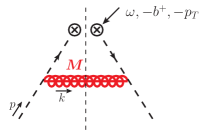
Refer to caption
Refer to caption
Refer to caption
Figure 20: Light-quark beam function diagrams for massive gluon radiation at one loop. In addition, also the wave function renormalization correction and the mirror diagrams for (b) and (c) have to be included in the calculation.
Contributions to the fully-differential beam function

As in sec. B.1 we start also here with the computation of the corrections for the fully-differential beam function. The contributing one-loop diagrams to the matrix element Bqqsubscript𝐵𝑞𝑞B_{qq} with massless quarks in the initial state, defined in analogy to eq. (134), are displayed in fig. 20. They consist of a purely virtual and a real-radiation part,

Bqq(1,bare)(t,pT,M,ω,z)=δ(1z)δ(t)δ(2)(pT)Bqq,virt(1,bare)(M,ω)+Bqq,real(1,bare)(t,pT,M,ω,z).subscriptsuperscript𝐵1bare𝑞𝑞𝑡subscript𝑝𝑇𝑀𝜔𝑧𝛿1𝑧𝛿𝑡superscript𝛿2subscript𝑝𝑇subscriptsuperscript𝐵1bare𝑞𝑞virt𝑀𝜔subscriptsuperscript𝐵1bare𝑞𝑞real𝑡subscript𝑝𝑇𝑀𝜔𝑧\displaystyle B^{(1,\rm bare)}_{qq}(t,\vec{p}_{T},M,\omega,z)=\delta(1-z)\,\delta(t)\,\delta^{(2)}(\vec{p}_{T})\,B^{(1,\rm bare)}_{qq,\rm{virt}}(M,\omega)+B^{(1,\rm bare)}_{qq,\rm{real}}(t,\vec{p}_{T},M,\omega,z)\;. (140)

The virtual massive gluon contributions in fig. 20 are the same as for other collinear quark operators like the current or the PDF and have been computed e.g. in ref. Chiu:2012ir . Including the wave function renormalization diagrams the d𝑑d-dimensional result reads Hoang:2015iva

Bqq,virt(1,bare)(M,ω)=CF(μ2eγEM2)ϵΓ(ϵ){4η+4lnνω+4H1ϵ2(1ϵ)2ϵ+𝒪(η)},subscriptsuperscript𝐵1bare𝑞𝑞virt𝑀𝜔subscript𝐶𝐹superscriptsuperscript𝜇2superscriptesubscript𝛾𝐸superscript𝑀2italic-ϵΓitalic-ϵ4𝜂4𝜈𝜔4subscript𝐻1italic-ϵ21italic-ϵ2italic-ϵ𝒪𝜂\displaystyle B^{(1,\rm{bare})}_{qq,\rm{virt}}(M,\omega)=C_{F}\,\Bigl{(}\frac{\mu^{2}\mathrm{e}^{\gamma_{E}}}{M^{2}}\Bigr{)}^{\epsilon}\Gamma(\epsilon)\,\biggl{\{}\frac{4}{\eta}+4\ln\frac{\nu}{\omega}+4H_{1-\epsilon}-\frac{2(1-\epsilon)}{2-\epsilon}+\mathcal{O}(\eta)\biggr{\}}\;, (141)

where Hα=ψ(1+α)+γEsubscript𝐻𝛼𝜓1𝛼subscript𝛾𝐸H_{\alpha}=\psi(1+\alpha)+\gamma_{E} is the Harmonic number. Here the rapidity divergences have been regulated using the symmetric η𝜂\eta regulator acting on the Wilson lines Chiu:2012ir ; Chiu:2011qc , while UV divergences are regulated with dimensional regularization as usual. Furthermore, the gluon mass provides an IR cutoff.

The real radiation contributions in figs. 20 and 20 can be easily evaluated, since all momentum components are fully determined by the measurement. For the first diagram we get

B(a)superscript𝐵𝑎\displaystyle B^{(a)} =8παsCFpθ(ω)θ(t)d4k(2π)4|k|2[(pk)2+iϵ]2δ(ωp+k)δ(tωk+)absent8𝜋subscript𝛼𝑠subscript𝐶𝐹superscript𝑝𝜃𝜔𝜃𝑡superscriptd4𝑘superscript2𝜋4superscriptsubscript𝑘perpendicular-to2superscriptdelimited-[]superscript𝑝𝑘2𝑖italic-ϵ2𝛿𝜔superscript𝑝superscript𝑘𝛿𝑡𝜔superscript𝑘\displaystyle=8\pi\alpha_{s}C_{F}p^{-}\theta(\omega)\,\theta(t)\int\frac{\mathrm{d}^{4}k}{(2\pi)^{4}}\,\frac{|\vec{k}_{\perp}|^{2}}{\big{[}(p-k)^{2}+i\epsilon\big{]}^{2}}\,\delta(\omega-p^{-}+k^{-})\,\delta(t-\omega k^{+})
×δ(2)(pTk) 2πδ(k2M2)absentsuperscript𝛿2subscript𝑝𝑇subscript𝑘perpendicular-to2𝜋𝛿superscript𝑘2superscript𝑀2\displaystyle\hskip 113.81102pt\times\delta^{(2)}(\vec{p}_{T}-\vec{k}_{\perp})\,2\pi\delta(k^{2}-M^{2})
=αsCF4π2θ(z)θ(t)δ(pT2t(1z)z+M2)2(t(1z)zM2)(tzM2)2.absentsubscript𝛼𝑠subscript𝐶𝐹4superscript𝜋2𝜃𝑧𝜃𝑡𝛿superscriptsubscript𝑝𝑇2𝑡1𝑧𝑧superscript𝑀22𝑡1𝑧𝑧superscript𝑀2superscript𝑡𝑧superscript𝑀22\displaystyle=\frac{\alpha_{s}C_{F}}{4\pi^{2}}\,\theta(z)\,\theta(t)\,\delta\Bigl{(}p_{T}^{2}-\frac{t(1-z)}{z}+M^{2}\Bigr{)}\,\frac{2\bigl{(}t(1-z)-zM^{2}\bigr{)}}{(t-zM^{2})^{2}}\;. (142)

Since UV divergences do not appear for the real radiation corrections and the gluon mass regulates all IR divergences we do not need to employ dimensional regularization here. The second diagram in fig. 20 yields

B(b)superscript𝐵𝑏\displaystyle B^{(b)} =8παsCFpθ(ω)θ(t)d4k(2π)4(pk)(pk)2+iϵνη(k)ηδ(ωp+k)δ(tωk+)absent8𝜋subscript𝛼𝑠subscript𝐶𝐹superscript𝑝𝜃𝜔𝜃𝑡superscriptd4𝑘superscript2𝜋4superscript𝑝superscript𝑘superscript𝑝𝑘2𝑖italic-ϵsuperscript𝜈𝜂superscriptsuperscript𝑘𝜂𝛿𝜔superscript𝑝superscript𝑘𝛿𝑡𝜔superscript𝑘\displaystyle=-8\pi\alpha_{s}C_{F}p^{-}\theta(\omega)\,\theta(t)\int\frac{\mathrm{d}^{4}k}{(2\pi)^{4}}\,\frac{(p^{-}-k^{-})}{(p-k)^{2}+i\epsilon}\,\frac{\nu^{\eta}}{(k^{-})^{\eta}}\,\delta(\omega-p^{-}+k^{-})\,\delta(t-\omega k^{+})
×δ(2)(pTk) 2πδ(k2M2)absentsuperscript𝛿2subscript𝑝𝑇subscript𝑘perpendicular-to2𝜋𝛿superscript𝑘2superscript𝑀2\displaystyle\hskip 113.81102pt\times\delta^{(2)}(\vec{p}_{T}-\vec{k}_{\perp})\,2\pi\delta(k^{2}-M^{2})
=αsCF4π2θ(z)θ(t)δ(pT2t(1z)z+M2)(νω)η2z1η(tzM2)(1z)η.absentsubscript𝛼𝑠subscript𝐶𝐹4superscript𝜋2𝜃𝑧𝜃𝑡𝛿superscriptsubscript𝑝𝑇2𝑡1𝑧𝑧superscript𝑀2superscript𝜈𝜔𝜂2superscript𝑧1𝜂𝑡𝑧superscript𝑀2superscript1𝑧𝜂\displaystyle=\frac{\alpha_{s}C_{F}}{4\pi^{2}}\,\theta(z)\,\theta(t)\,\delta\Bigl{(}p_{T}^{2}-\frac{t(1-z)}{z}+M^{2}\Bigr{)}\Bigl{(}\frac{\nu}{\omega}\Bigr{)}^{\eta}\frac{2z^{1-\eta}}{(t-zM^{2})(1-z)^{\eta}}\,. (143)

While the fully-differential quark beam function itself does not contain any rapidity divergences, we have included here the η𝜂\eta regulator, since we will use this result to obtain the TMD beam function by integrating over the virtuality, which results in rapidity divergences for this real radiation correction. The full real radiation contributions at one loop yield

αs4πBqq,real(1,bare)(t,pT,M,ω,z)subscript𝛼𝑠4𝜋superscriptsubscript𝐵𝑞𝑞real1bare𝑡subscript𝑝𝑇𝑀𝜔𝑧\displaystyle\frac{\alpha_{s}}{4\pi}B_{qq,\rm{real}}^{(1,\rm{bare})}(t,\vec{p}_{T},M,\omega,z) =B(a)+2B(b)absentsuperscript𝐵𝑎2superscript𝐵𝑏\displaystyle=B^{(a)}+2B^{(b)}
=αsCF4π1πθ(z)θ(t)δ(pT2t(1z)z+M2)absentsubscript𝛼𝑠subscript𝐶𝐹4𝜋1𝜋𝜃𝑧𝜃𝑡𝛿superscriptsubscript𝑝𝑇2𝑡1𝑧𝑧superscript𝑀2\displaystyle=\frac{\alpha_{s}C_{F}}{4\pi}\,\frac{1}{\pi}\,\theta(z)\,\theta(t)\,\delta\Bigl{(}p_{T}^{2}-\frac{t(1-z)}{z}+M^{2}\Bigr{)}
×2tzM2[(νω)η2z1η(1z)η+t(1z)zM2tzM2].absent2𝑡𝑧superscript𝑀2delimited-[]superscript𝜈𝜔𝜂2superscript𝑧1𝜂superscript1𝑧𝜂𝑡1𝑧𝑧superscript𝑀2𝑡𝑧superscript𝑀2\displaystyle\quad\times\frac{2}{t-zM^{2}}\biggl{[}\Bigl{(}\frac{\nu}{\omega}\Bigr{)}^{\eta}\frac{2z^{1-\eta}}{(1-z)^{\eta}}+\frac{t(1-z)-zM^{2}}{t-zM^{2}}\biggr{]}\,. (144)

For both virtual and real radiation corrections all soft-bin subtractions are parametrically power suppressed or scaleless and therefore do not contribute.

Contributions to the TMD beam function

The corrections for the TMD beam function with a massive gluon can be obtained by integrating the fully-differential beam function in eq. (140) over the virtuality t𝑡t. We write them again as

Bqq(1,bare)(pT,M,z)=δ(1z)δ(2)(pT)Bqq,virt(1,bare)(M,ω)+Bqq,real(1,bare)(pT,M,ω,z),superscriptsubscript𝐵𝑞𝑞1baresubscript𝑝𝑇𝑀𝑧𝛿1𝑧superscript𝛿2subscript𝑝𝑇subscriptsuperscript𝐵1bare𝑞𝑞virt𝑀𝜔subscriptsuperscript𝐵1bare𝑞𝑞realsubscript𝑝𝑇𝑀𝜔𝑧\displaystyle B_{qq}^{(1,\rm{bare})}(\vec{p}_{T},M,z)=\delta(1-z)\,\delta^{(2)}(\vec{p}_{T})\,B^{(1,\rm{bare})}_{qq,\rm{virt}}(M,\omega)+B^{(1,\rm{bare})}_{qq,\rm{real}}(\vec{p}_{T},M,\omega,z)\;, (145)

where Bqq,virt(1,bare)subscriptsuperscript𝐵1bare𝑞𝑞virtB^{(1,\rm{bare})}_{qq,\rm{virt}} is given in eq. (141) and

Bqq,real(1,bare)(pT,M,ω,z)superscriptsubscript𝐵𝑞𝑞real1baresubscript𝑝𝑇𝑀𝜔𝑧\displaystyle B_{qq,\rm{real}}^{(1,\rm{bare})}(\vec{p}_{T},M,\omega,z) =dtBqq,real(1,bare)(t,pT,M,z)absentdifferential-d𝑡superscriptsubscript𝐵𝑞𝑞real1bare𝑡subscript𝑝𝑇𝑀𝑧\displaystyle=\int\mathrm{d}t\,B_{qq,\rm{real}}^{(1,\rm{bare})}(t,\vec{p}_{T},M,z) (146)
=CFθ(z)θ(1z)1π2pT2+zM2[pT2(1z)pT2+zM2+2z1η(1z)1+η(νω)η].absentsubscript𝐶𝐹𝜃𝑧𝜃1𝑧1𝜋2superscriptsubscript𝑝𝑇2𝑧superscript𝑀2delimited-[]superscriptsubscript𝑝𝑇21𝑧superscriptsubscript𝑝𝑇2𝑧superscript𝑀22superscript𝑧1𝜂superscript1𝑧1𝜂superscript𝜈𝜔𝜂\displaystyle=C_{F}\,\theta(z)\,\theta(1-z)\,\frac{1}{\pi}\,\frac{2}{p_{T}^{2}+zM^{2}}\biggl{[}\frac{p_{T}^{2}(1-z)}{p_{T}^{2}+zM^{2}}+\frac{2z^{1-\eta}}{(1-z)^{1+\eta}}\Bigl{(}\frac{\nu}{\omega}\Bigr{)}^{\eta}\biggr{]}\;.

Here it is necessary to keep a nonvanishing value for η𝜂\eta in the second term to regularize the rapidity divergence for z1𝑧1z\to 1. Expanding for η0𝜂0\eta\to 0 we get

Bqq,real(1,bare)(pT,M,ω,z)superscriptsubscript𝐵𝑞𝑞real1baresubscript𝑝𝑇𝑀𝜔𝑧\displaystyle B_{qq,\rm{real}}^{(1,\rm{bare})}(\vec{p}_{T},M,\omega,z) =CFθ(z)1π{4pT2+M2[δ(1z)(1η+lnνω)+0(1z)]\displaystyle=C_{F}\,\theta(z)\,\frac{1}{\pi}\,\biggl{\{}\frac{4}{p_{T}^{2}+M^{2}}\Bigl{[}-\delta(1-z)\Bigl{(}\frac{1}{\eta}+\ln\frac{\nu}{\omega}\Bigr{)}+\mathcal{L}_{0}(1-z)\Bigr{]}
+θ(1z)2pT2pT2+zM2[1zpT2+zM22pT2+M2]}+𝒪(η).\displaystyle+\theta(1-z)\frac{2p_{T}^{2}}{p_{T}^{2}+zM^{2}}\Bigl{[}\frac{1-z}{p_{T}^{2}+zM^{2}}-\frac{2}{p_{T}^{2}+M^{2}}\Bigr{]}\biggr{\}}+\mathcal{O}(\eta)\;. (147)
Contributions to the virtuality-dependent beam function

The virtuality-dependent beam function with a massive gluon can be obtained by integrating the results for the fully-differential beam function over pTsubscript𝑝𝑇\vec{p}_{T}. We decompose the corrections again into a virtual and real radiation part,

Bqq(1,bare)(t,M,z)=δ(1z)δ(t)Bqq,virt(1,bare)(M,ω)+Bqq,real(1,bare)(t,M,z),superscriptsubscript𝐵𝑞𝑞1bare𝑡𝑀𝑧𝛿1𝑧𝛿𝑡subscriptsuperscript𝐵1bare𝑞𝑞virt𝑀𝜔subscriptsuperscript𝐵1bare𝑞𝑞real𝑡𝑀𝑧\displaystyle B_{qq}^{(1,\rm{bare})}(t,M,z)=\delta(1-z)\,\delta(t)\,B^{(1,\rm{bare})}_{qq,\rm{virt}}(M,\omega)+B^{(1,\rm{bare})}_{qq,\rm{real}}(t,M,z)\;, (148)

where Bqq,virt(1,bare)subscriptsuperscript𝐵1bare𝑞𝑞virtB^{(1,\rm{bare})}_{qq,\rm{virt}} is given in eq. (141) and

Bqq,real(1)(t,M,z)superscriptsubscript𝐵𝑞𝑞real1𝑡𝑀𝑧\displaystyle B_{qq,\rm{real}}^{(1)}(t,M,z) =d2pTBqq,real(1,bare)(t,pT,M,ω,z)absentsuperscriptd2subscript𝑝𝑇superscriptsubscript𝐵𝑞𝑞real1bare𝑡subscript𝑝𝑇𝑀𝜔𝑧\displaystyle=\int\mathrm{d}^{2}\vec{p}_{T}\,B_{qq,\rm{real}}^{(1,\rm{bare})}(t,\vec{p}_{T},M,\omega,z) (149)
=CFθ(z)θ(t)θ(t(1z)zM2)2tzM2(2z1z+t(1z)zM2tzM2),absentsubscript𝐶𝐹𝜃𝑧𝜃𝑡𝜃𝑡1𝑧𝑧superscript𝑀22𝑡𝑧superscript𝑀22𝑧1𝑧𝑡1𝑧𝑧superscript𝑀2𝑡𝑧superscript𝑀2\displaystyle=C_{F}\,\theta(z)\,\theta(t)\,\theta\Bigl{(}\frac{t(1-z)}{z}-M^{2}\Bigr{)}\,\frac{2}{t-zM^{2}}\Bigl{(}\frac{2z}{1-z}+\frac{t(1-z)-zM^{2}}{t-zM^{2}}\Bigr{)}\,,

with the fully-differential real radiation contributions in eq. (144). Here the η𝜂\eta regulator has already been dropped, since for the virtuality-dependent beam function no rapidity divergences arise from the real radiation contributions.

B.3.2 Secondary massive quark effects in the TMD beam function

To obtain the secondary massive quark corrections from the one-loop results with a massive gluon, we first convolve the one-loop results with the imaginary part of the vacuum polarization function according to eq. (B.2) and define

αsTF4πBqq,virt(2,h,bare)(m,ω)subscript𝛼𝑠subscript𝑇𝐹4𝜋subscriptsuperscript𝐵2bare𝑞𝑞virt𝑚𝜔\displaystyle\frac{\alpha_{s}T_{F}}{4\pi}B^{(2,h,\rm{bare})}_{qq,\rm{virt}}(m,\omega) =1πdM2M2Im[Π(m2,M2)]×Bqq,virt(1,bare)(M,ω),absent1𝜋dsuperscript𝑀2superscript𝑀2Imdelimited-[]Πsuperscript𝑚2superscript𝑀2subscriptsuperscript𝐵1bare𝑞𝑞virt𝑀𝜔\displaystyle=\frac{1}{\pi}\int\frac{\mathrm{d}M^{2}}{M^{2}}\,{\rm{Im}}\bigl{[}\Pi(m^{2},M^{2})\bigr{]}\times B^{(1,\rm{bare})}_{qq,\rm{virt}}(M,\omega)\;,
αsTF4πBqq,real(2,h,bare)(pT,m,ω,z)subscript𝛼𝑠subscript𝑇𝐹4𝜋subscriptsuperscript𝐵2bare𝑞𝑞realsubscript𝑝𝑇𝑚𝜔𝑧\displaystyle\frac{\alpha_{s}T_{F}}{4\pi}B^{(2,h,\rm{bare})}_{qq,\rm{real}}(\vec{p}_{T},m,\omega,z) =1πdM2M2Im[Π(m2,M2)]×Bqq,real(1,bare)(pT,M,ω,z).absent1𝜋dsuperscript𝑀2superscript𝑀2Imdelimited-[]Πsuperscript𝑚2superscript𝑀2subscriptsuperscript𝐵1bare𝑞𝑞realsubscript𝑝𝑇𝑀𝜔𝑧\displaystyle=\frac{1}{\pi}\int\frac{\mathrm{d}M^{2}}{M^{2}}\,{\rm{Im}}\bigl{[}\Pi(m^{2},M^{2})\bigr{]}\times B^{(1,\rm{bare})}_{qq,\rm{real}}(\vec{p}_{T},M,\omega,z)\;. (150)

The results from these dispersion integrations are

Bqq,virt(2,h,bare)(m,ω)subscriptsuperscript𝐵2bare𝑞𝑞virt𝑚𝜔\displaystyle B^{(2,h,\rm{bare})}_{qq,\rm{virt}}(m,\omega) =CF{(1η+lnνω)[83ϵ21ϵ(163Lm+409)+163Lm2+809Lm+22427\displaystyle=C_{F}\,\biggl{\{}\Bigl{(}\frac{1}{\eta}+\ln\frac{\nu}{\omega}\Bigr{)}\biggl{[}\frac{8}{3\epsilon^{2}}-\frac{1}{\epsilon}\Bigl{(}\frac{16}{3}L_{m}+\frac{40}{9}\Bigr{)}+\frac{16}{3}L_{m}^{2}+\frac{80}{9}L_{m}+\frac{224}{27}
+4π29+𝒪(ϵ)]+2ϵ21ϵ(4Lm+13+4π29)+4Lm2+(23+8π29)Lm\displaystyle\quad+\frac{4\pi^{2}}{9}+\mathcal{O}(\epsilon)\biggr{]}+\frac{2}{\epsilon^{2}}-\frac{1}{\epsilon}\Bigl{(}4L_{m}+\frac{1}{3}+\frac{4\pi^{2}}{9}\Bigr{)}+4L_{m}^{2}+\Bigl{(}\frac{2}{3}+\frac{8\pi^{2}}{9}\Bigr{)}L_{m}
+7318+29π2278ζ33},\displaystyle\quad+\frac{73}{18}+\frac{29\pi^{2}}{27}-\frac{8\zeta_{3}}{3}\biggr{\}}\;, (151)
Bqq,real(2,h,bare)(pT,m,ω,z)subscriptsuperscript𝐵2bare𝑞𝑞realsubscript𝑝𝑇𝑚𝜔𝑧\displaystyle B^{(2,h,\rm{bare})}_{qq,\rm{real}}(\vec{p}_{T},m,\omega,z) =CF1πpT2{169ηδ(1z)[512m^23c(12m^2)ln(c+1c1)]\displaystyle=C_{F}\,\frac{1}{\pi p_{T}^{2}}\biggl{\{}\frac{16}{9\eta}\,\delta(1-z)\biggl{[}5-12\hat{m}^{2}-3c(1-2\hat{m}^{2})\ln\Bigl{(}\frac{c+1}{c-1}\Bigr{)}\biggr{]}
+brealqT(m2pT2,z,νω)},\displaystyle\quad+b_{\rm{real}}^{q_{T}}\Bigl{(}\frac{m^{2}}{p_{T}^{2}},z,\frac{\nu}{\omega}\Bigr{)}\biggr{\}}\;, (152)

with

brealqT(m^2,z,νω)=θ(z)169{[512m^23c(12m^2)ln(c+1c1)]\displaystyle b_{\rm{real}}^{q_{T}}\Bigl{(}\hat{m}^{2},z,\frac{\nu}{\omega}\Bigr{)}=\theta(z)\frac{16}{9}\biggl{\{}\biggl{[}5-12\hat{m}^{2}-3c(1-2\hat{m}^{2})\ln\Bigl{(}\frac{c+1}{c-1}\Bigr{)}\biggr{]}
×(δ(1z)lnνω0(1z))absent𝛿1𝑧𝜈𝜔subscript01𝑧\displaystyle\qquad\times\Bigl{(}\delta(1-z)\ln\frac{\nu}{\omega}-\mathcal{L}_{0}(1-z)\Bigr{)}
+θ(1z)[32d(1z)[1+z2+2m^2z(1+z2)+4m^4z2(5+6z5z2)]ln(d+1d1)\displaystyle\qquad+\theta(1-z)\biggl{[}\frac{3}{2d(1-z)}\bigl{[}1+z^{2}+2\hat{m}^{2}z(1+z^{2})+4\hat{m}^{4}z^{2}(-5+6z-5z^{2})\bigr{]}\,\ln\Bigl{(}\frac{d+1}{d-1}\Bigr{)}
3c(12m^2)1zln(c+1c1)+1+4z+3m^2(4+z5z2)]},\displaystyle\qquad-\frac{3c(1-2\hat{m}^{2})}{1-z}\ln\Bigl{(}\frac{c+1}{c-1}\Bigr{)}+1+4z+3\hat{m}^{2}(-4+z-5z^{2})\biggr{]}\biggr{\}}\;, (153)

and m^^𝑚\hat{m}, c𝑐c, d𝑑d defined in eq. (66). Using eq. (B.3.2) entails that the massive quark corrections to the strong coupling are renormalized in the on-shell scheme, i.e., the expansion is in terms of αs=αs(nl)subscript𝛼𝑠superscriptsubscript𝛼𝑠subscript𝑛𝑙\alpha_{s}=\alpha_{s}^{(n_{l})}. Since the beam function matrix element has to be renormalized entirely in the nl+1subscript𝑛𝑙1n_{l}+1 flavor theory, we need to account for the second term in eq. (B.2) (which switches back to an unrenormalized αssubscript𝛼𝑠\alpha_{s}) and renormalize the massive quark corrections to the strong coupling in the MS¯¯MS\overline{\rm MS} scheme, such that the expansion is in terms of αs=αs(nl+1)subscript𝛼𝑠superscriptsubscript𝛼𝑠subscript𝑛𝑙1\alpha_{s}=\alpha_{s}^{(n_{l}+1)}. The beam function operator is renormalized according to

𝒪q(bare)(pT,m,ω)=d2pTZB(pTpT,m,μ,νω)𝒪q(pT,m,ω,μ,ν),subscriptsuperscript𝒪bare𝑞subscript𝑝𝑇𝑚𝜔superscriptd2superscriptsubscript𝑝𝑇subscript𝑍𝐵subscript𝑝𝑇subscriptsuperscript𝑝𝑇𝑚𝜇𝜈𝜔subscript𝒪𝑞subscriptsuperscript𝑝𝑇𝑚𝜔𝜇𝜈\displaystyle\mathcal{O}^{(\rm bare)}_{q}(\vec{p}_{T},m,\omega)=\int\textrm{d}^{2}p_{T}^{\prime}\,Z_{B}\Bigl{(}\vec{p}_{T}-\vec{p}^{\,\prime}_{T},m,\mu,\frac{\nu}{\omega}\Bigr{)}\,\mathcal{O}_{q}(\vec{p}^{\,\prime}_{T},m,\omega,\mu,\nu)\,, (154)

where the counterterm encodes also the rapidity divergences. This yields for the renormalized matrix element with initial state quarks at 𝒪(αs2CFTF)𝒪superscriptsubscript𝛼𝑠2subscript𝐶𝐹subscript𝑇𝐹\mathcal{O}(\alpha_{s}^{2}C_{F}T_{F}) in terms of αs=αs(nl+1)subscript𝛼𝑠superscriptsubscript𝛼𝑠subscript𝑛𝑙1\alpha_{s}=\alpha_{s}^{(n_{l}+1)}

Bqq(2,h)(pT,m,z,μ,νω)superscriptsubscript𝐵𝑞𝑞2subscript𝑝𝑇𝑚𝑧𝜇𝜈𝜔\displaystyle B_{qq}^{(2,h)}\Bigl{(}\vec{p}_{T},m,z,\mu,\frac{\nu}{\omega}\Bigr{)} =δ(2)(pT)δ(1z)Bqq,virt(2,h,bare)(m,ω)+Bqq,real(2,h,bare)(pT,m,ω,z)absentsuperscript𝛿2subscript𝑝𝑇𝛿1𝑧subscriptsuperscript𝐵2bare𝑞𝑞virt𝑚𝜔subscriptsuperscript𝐵2bare𝑞𝑞realsubscript𝑝𝑇𝑚𝜔𝑧\displaystyle=\delta^{(2)}(\vec{p}_{T})\,\delta(1-z)\,B^{(2,h,\rm{bare})}_{qq,\rm{virt}}(m,\omega)+B^{(2,h,\rm{bare})}_{qq,\rm{real}}(\vec{p}_{T},m,\omega,z) (155)
(Π(1)(m2,0)43ϵ)Bqq(1,bare)(pT,ω,z)=Bqq(1)(pT,z,μ,νω)+ZB(1)(pT,μ,νω)δ(1z)δ(1z)ZB(2,h)(pT,m,μ,νω).\displaystyle\quad-\Bigl{(}\Pi^{(1)}(m^{2},0)-\frac{4}{3\epsilon}\Bigr{)}\underbrace{B_{qq}^{(1,\rm bare)}(\vec{p}_{T},\omega,z)}_{\makebox[0.0pt]{\scriptsize$=B^{(1)}_{qq}(\vec{p}_{T},z,\mu,\frac{\nu}{\omega})+Z_{B}^{(1)}(\vec{p}_{T},\mu,\frac{\nu}{\omega})\,\delta(1-z)$}}-\delta(1-z)Z_{B}^{(2,h)}\Bigl{(}\vec{p}_{T},m,\mu,\frac{\nu}{\omega}\Bigl{)}\,.

where the (bare) vacuum polarization function Π(1)(m2,0)superscriptΠ1superscript𝑚20\Pi^{(1)}(m^{2},0) is given in eq. (139). The one-loop counterterm reads

ZB(1)(pT,μ,νω)=CF{δ(2)(pT)[1η(4ϵ+𝒪(ϵ))+1ϵ(3+4lnνω)]1η(4+𝒪(ϵ))0(pT,μ)}.superscriptsubscript𝑍𝐵1subscript𝑝𝑇𝜇𝜈𝜔subscript𝐶𝐹superscript𝛿2subscript𝑝𝑇delimited-[]1𝜂4italic-ϵ𝒪italic-ϵ1italic-ϵ34𝜈𝜔1𝜂4𝒪italic-ϵsubscript0subscript𝑝𝑇𝜇\displaystyle Z_{B}^{(1)}\Bigl{(}\vec{p}_{T},\mu,\frac{\nu}{\omega}\Bigr{)}=C_{F}\,\biggl{\{}\delta^{(2)}(\vec{p}_{T})\biggl{[}\frac{1}{\eta}\Bigl{(}\frac{4}{\epsilon}+\mathcal{O}(\epsilon)\Bigr{)}+\frac{1}{\epsilon}\Bigl{(}3+4\ln\frac{\nu}{\omega}\Bigr{)}\biggr{]}-\frac{1}{\eta}\Bigl{(}4+\mathcal{O}(\epsilon)\Bigr{)}\mathcal{L}_{0}(\vec{p}_{T},\mu)\biggr{\}}\;. (156)

The two-loop counterterm ZB(2)superscriptsubscript𝑍𝐵2Z_{B}^{(2)} absorbs all remaining UV and rapidity divergences in eq. (155) and is given by

ZB(2,h)(pT,m,μ,νω)=CF{δ(2)(pT)[1η(83ϵ2409ϵ+83Lm2+809Lm+22427+𝒪(ϵ))\displaystyle Z_{B}^{(2,h)}\Bigl{(}\vec{p}_{T},m,\mu,\frac{\nu}{\omega}\Bigr{)}=C_{F}\,\biggl{\{}\delta^{(2)}(\vec{p}_{T})\biggl{[}\frac{1}{\eta}\Bigl{(}\frac{8}{3\epsilon^{2}}-\frac{40}{9\epsilon}+\frac{8}{3}L_{m}^{2}+\frac{80}{9}L_{m}+\frac{224}{27}+\mathcal{O}(\epsilon)\Bigr{)}
+1ϵ2(2+83lnνω)1ϵ(13+4π29+409lnνω)]1η(163Lm+𝒪(ϵ))0(pT,μ)\displaystyle\qquad+\frac{1}{\epsilon^{2}}\Bigl{(}2+\frac{8}{3}\ln\frac{\nu}{\omega}\Bigr{)}-\frac{1}{\epsilon}\Bigl{(}\frac{1}{3}+\frac{4\pi^{2}}{9}+\frac{40}{9}\ln\frac{\nu}{\omega}\Bigr{)}\biggr{]}-\frac{1}{\eta}\Bigl{(}\frac{16}{3}L_{m}+\mathcal{O}(\epsilon)\Bigr{)}\mathcal{L}_{0}(\vec{p}_{T},\mu)
+1η169πpT2[512m^23c(12m^2)lnc+1c1]}.\displaystyle\qquad+\frac{1}{\eta}\,\frac{16}{9\pi p_{T}^{2}}\biggl{[}5-12\hat{m}^{2}-3c(1-2\hat{m}^{2})\ln\frac{c+1}{c-1}\biggr{]}\biggr{\}}\,. (157)

This yields the anomalous dimensions in eq. (4.2.1). The renormalized one-loop partonic beam function Bqq(1)superscriptsubscript𝐵𝑞𝑞1B_{qq}^{(1)} still contains IR divergences, so its exact form depends on the choice of the IR regulator.

The beam function matching coefficient qqsubscript𝑞𝑞\mathcal{I}_{qq} as defined in (14) can be now easily obtained. Note that the PDFs are renormalized in an nlsubscript𝑛𝑙n_{l}-flavor theory with αs=αs(nl)subscript𝛼𝑠superscriptsubscript𝛼𝑠subscript𝑛𝑙\alpha_{s}=\alpha_{s}^{(n_{l})} in contrast to the beam function. Thus, there is a contribution coming from the scheme change of αssubscript𝛼𝑠\alpha_{s} to nl+1subscript𝑛𝑙1n_{l}+1 flavors for the (renormalized) one-loop PDF correction, i.e.

qq(2,h)(pT,m,z,μ,νω)superscriptsubscript𝑞𝑞2subscript𝑝𝑇𝑚𝑧𝜇𝜈𝜔\displaystyle\mathcal{I}_{qq}^{(2,h)}\Bigl{(}\vec{p}_{T},m,z,\mu,\frac{\nu}{\omega}\Bigr{)} =Bqq(2,h)(pT,m,z,μ,νω)δ(2)(pT)43Lmfqq(1)(z,μ)absentsuperscriptsubscript𝐵𝑞𝑞2subscript𝑝𝑇𝑚𝑧𝜇𝜈𝜔superscript𝛿2subscript𝑝𝑇43subscript𝐿𝑚superscriptsubscript𝑓𝑞𝑞1𝑧𝜇\displaystyle=B_{qq}^{(2,h)}\Bigl{(}\vec{p}_{T},m,z,\mu,\frac{\nu}{\omega}\Bigr{)}-\delta^{(2)}(\vec{p}_{T})\,\frac{4}{3}L_{m}f_{qq}^{(1)}(z,\mu)
=δ(2)(pT)δ(1z)Bqq,virt(2,h,bare)(m,ω)+Bqq,real(2,h,bare)(pT,m,ω,z)absentsuperscript𝛿2subscript𝑝𝑇𝛿1𝑧subscriptsuperscript𝐵2bare𝑞𝑞virt𝑚𝜔subscriptsuperscript𝐵2bare𝑞𝑞realsubscript𝑝𝑇𝑚𝜔𝑧\displaystyle=\delta^{(2)}(\vec{p}_{T})\,\delta(1-z)B^{(2,h,\rm{bare})}_{qq,\rm{virt}}(m,\omega)+B^{(2,h,\rm{bare})}_{qq,\rm{real}}(\vec{p}_{T},m,\omega,z)
δ(1z)[(Π(1)(m2,0)43ϵ)ZB(1)(pT,μ,νω)+ZB(2,h)(pT,m,μ,νω)]\displaystyle\quad-\delta(1-z)\biggl{[}\Bigl{(}\Pi^{(1)}(m^{2},0)-\frac{4}{3\epsilon}\Bigr{)}\,Z_{B}^{(1)}\Bigl{(}\vec{p}_{T},\mu,\frac{\nu}{\omega}\Bigr{)}+Z_{B}^{(2,h)}\Bigl{(}\vec{p}_{T},m,\mu,\frac{\nu}{\omega}\Bigl{)}\biggr{]}
+43Lm(Bqq(1)(pT,z,μ,νω)δ(2)(pT)fqq(1)(z,μ))=qq(1)(pT,z,μ,νω).43subscript𝐿𝑚subscriptsubscriptsuperscript𝐵1𝑞𝑞subscript𝑝𝑇𝑧𝜇𝜈𝜔superscript𝛿2subscript𝑝𝑇superscriptsubscript𝑓𝑞𝑞1𝑧𝜇absentsuperscriptsubscript𝑞𝑞1subscript𝑝𝑇𝑧𝜇𝜈𝜔\displaystyle\quad+\frac{4}{3}L_{m}\underbrace{\biggl{(}B^{(1)}_{qq}\Bigl{(}\vec{p}_{T},z,\mu,\frac{\nu}{\omega}\Bigr{)}-\delta^{(2)}(\vec{p}_{T})f_{qq}^{(1)}(z,\mu)\biggr{)}}_{=\,\mathcal{I}_{qq}^{(1)}(\vec{p}_{T},z,\mu,\frac{\nu}{\omega})}\,. (158)

Here the IR divergences cancel between the one-loop beam function and the PDF to give the finite one-loop matching coefficient qq(1)superscriptsubscript𝑞𝑞1\mathcal{I}_{qq}^{(1)}, which is given in eq. (119). Using eqs. (151), (152), (156) and (B.3.2) we obtain the full result for the secondary massive quark corrections to the beam function matching coefficient given in eq. (4.2.1).

B.3.3 Secondary massive quark effects in the virtuality-dependent beam function

We proceed with the virtuality-dependent beam function. While the virtual contributions are the same as for the TMD beam function given in eq. (151), the dispersion integration for the real radiation terms yields

αsTF4πBqq,real(2,h)(t,m,z)subscript𝛼𝑠subscript𝑇𝐹4𝜋subscriptsuperscript𝐵2𝑞𝑞real𝑡𝑚𝑧\displaystyle\frac{\alpha_{s}T_{F}}{4\pi}B^{(2,h)}_{qq,\rm{real}}(t,m,z) =1πdM2M2Im[Π(m2,M2)]×Bqq,real(1)(t,M,z)absent1𝜋dsuperscript𝑀2superscript𝑀2Imdelimited-[]Πsuperscript𝑚2superscript𝑀2subscriptsuperscript𝐵1𝑞𝑞real𝑡𝑀𝑧\displaystyle=\frac{1}{\pi}\int\frac{\mathrm{d}M^{2}}{M^{2}}\,{\rm{Im}}\bigl{[}\Pi(m^{2},M^{2})\bigr{]}\times B^{(1)}_{qq,\rm{real}}(t,M,z)
=αsTF4πCFtbreal𝒯(m2t,z),absentsubscript𝛼𝑠subscript𝑇𝐹4𝜋subscript𝐶𝐹𝑡superscriptsubscript𝑏real𝒯superscript𝑚2𝑡𝑧\displaystyle=\frac{\alpha_{s}T_{F}}{4\pi}\,\frac{C_{F}}{t}\,b_{\rm{real}}^{{\mathcal{T}}}\Bigl{(}\frac{m^{2}}{t},z\Bigr{)}\,, (159)

with

breal𝒯(m^2,z)superscriptsubscript𝑏real𝒯superscript^𝑚2𝑧\displaystyle b_{\rm{real}}^{{\mathcal{T}}}(\hat{m}^{2},z) =θ(z)θ(v)89(1z){3ulnuvu+v[1+z22m^t2z(1+z2)4m^t4z2(23z+5z2)]\displaystyle=\theta(z)\,\theta(v)\,\frac{8}{9(1-z)}\biggl{\{}-\frac{3}{u}\ln\frac{u-v}{u+v}\biggl{[}1+z^{2}-2\hat{m}_{t}^{2}z(1+z^{2})-4\hat{m}_{t}^{4}z^{2}(2-3z+5z^{2})\biggr{]}
2v[43z+4z2+z(1121z+29z215z3)1zm^t2]},\displaystyle\quad-2v\biggl{[}4-3z+4z^{2}+\frac{z(11-21z+29z^{2}-15z^{3})}{1-z}\,\hat{m}_{t}^{2}\biggr{]}\biggr{\}}\,, (160)

and m^tsubscript^𝑚𝑡\hat{m}_{t}, u𝑢u, v𝑣v as in eq. (71).

To obtain the quark mass dependent matching coefficient qq(2,h)subscriptsuperscript2𝑞𝑞\mathcal{I}^{(2,h)}_{qq} we carry out our calculation using a gluon mass ΛQ𝒯mmuch-less-thanΛ𝑄𝒯similar-to𝑚\Lambda\ll\sqrt{Q{\mathcal{T}}}\sim m as IR regulator. Although the result is independent of the regulator, this is technically most convenient, since this allows us to match two SCETIIsubscriptSCETII{\rm SCET}_{\rm II} theories with each other in a straightforward way.777Alternatively, one can also perform the matching between theories where the fluctuations related to the nlsubscript𝑛𝑙n_{l} massless flavors are described within a SCETIsubscriptSCETI{\rm SCET}_{\rm I} theory. In this setup, there is no csoft function on the right-hand side of the matching relation in contrast to eq. (161). However, in this case the zero-bin subtractions for the collinear fields with respect to the ultrasoft modes in the SCETIsubscriptSCETI{\rm SCET}_{\rm I} nlsubscript𝑛𝑙n_{l} flavor theory yield a nontrivial contribution to the beam-function matrix element on the left-hand side of the matching relation. Their contribution is equivalent to the inverse of the csoft function in eq. (161), such that the resulting matching coefficient qqsubscript𝑞𝑞\mathcal{I}_{qq} is the same. While the SCETIIsubscriptSCETII{\rm SCET}_{\rm II} theory with nl+1subscript𝑛𝑙1n_{l}+1 flavors (i.e. above the mass scale) contains collinear modes, the SCETIIsubscriptSCETII{\rm SCET}_{\rm II} theory with nlsubscript𝑛𝑙n_{l} flavors (i.e. below the mass scale) contains collinear and csoft modes like in the mode setup of sec. 3.3. The matching relation reads

qq(nl+1)(t,m,z,μ,νω)=dqq(tω,m,z,μ,νω)zfqq(nl)(z,μ)𝒮(nl)(,μ,ν),superscriptsubscript𝑞𝑞subscript𝑛𝑙1𝑡𝑚𝑧𝜇𝜈𝜔subscripttensor-product𝑧differential-dsubscript𝑞𝑞𝑡𝜔𝑚𝑧𝜇𝜈𝜔subscriptsuperscript𝑓subscript𝑛𝑙𝑞𝑞𝑧𝜇superscript𝒮subscript𝑛𝑙𝜇𝜈\displaystyle\mathscr{B}_{qq}^{(n_{l}+1)}\Bigl{(}t,m,z,\mu,\frac{\nu}{\omega}\Bigr{)}=\int\mathrm{d}\ell\,\mathcal{I}_{qq}\Bigl{(}t-\omega\ell,m,z,\mu,\frac{\nu}{\omega}\Bigr{)}\otimes_{z}f^{(n_{l})}_{qq}(z,\mu)\,\mathscr{S}^{(n_{l})}(\ell,\mu,\nu)\;, (161)

where qq(nl+1)superscriptsubscript𝑞𝑞subscript𝑛𝑙1\mathscr{B}_{qq}^{(n_{l}+1)} corresponds to the pure SCETIIsubscriptSCETII{\rm SCET}_{\rm II} beam function matrix element and 𝒮(nl)superscript𝒮subscript𝑛𝑙\mathscr{S}^{(n_{l})} represents the csoft matrix element.

In close analogy to eq. (155) the renormalized SCETIIsubscriptSCETII{\rm SCET}_{\rm II} matrix element qq(nl+1)superscriptsubscript𝑞𝑞subscript𝑛𝑙1\mathscr{B}_{qq}^{(n_{l}+1)} is given at 𝒪(αs2CFTF)𝒪superscriptsubscript𝛼𝑠2subscript𝐶𝐹subscript𝑇𝐹\mathcal{O}(\alpha_{s}^{2}C_{F}T_{F}) by

qq(2,h)(t,m,z,μ,νω)superscriptsubscript𝑞𝑞2𝑡𝑚𝑧𝜇𝜈𝜔\displaystyle\mathscr{B}_{qq}^{(2,h)}\Bigl{(}t,m,z,\mu,\frac{\nu}{\omega}\Bigr{)} =δ(t)δ(1z)Bqq,virt(2,h,bare)(m,ω)+Bqq,real(2,h)(t,m,z)absent𝛿𝑡𝛿1𝑧subscriptsuperscript𝐵2bare𝑞𝑞virt𝑚𝜔subscriptsuperscript𝐵2𝑞𝑞real𝑡𝑚𝑧\displaystyle=\delta(t)\,\delta(1-z)\,B^{(2,h,\rm{bare})}_{qq,\rm{virt}}(m,\omega)+B^{(2,h)}_{qq,\rm{real}}(t,m,z) (162)
(Π(1)(m2,0)43ϵ)Bqq(1,bare)(t,z)=qq(1)(t,z,μ,νω)+Z(1)(t,μ,νω)δ(1z)δ(1z)Z(2,h)(t,m,μ,νω).\displaystyle\quad-\Bigl{(}\Pi^{(1)}(m^{2},0)-\frac{4}{3\epsilon}\Bigr{)}\underbrace{B_{qq}^{(1,\rm bare)}(t,z)}_{\makebox[0.0pt]{\scriptsize$=\mathscr{B}^{(1)}_{qq}(t,z,\mu,\frac{\nu}{\omega})+Z_{\mathscr{B}}^{(1)}(t,\mu,\frac{\nu}{\omega})\,\delta(1-z)$}}-\,\delta(1-z)Z_{\mathscr{B}}^{(2,h)}\Bigl{(}t,m,\mu,\frac{\nu}{\omega}\Bigl{)}\,.

To separate UV, rapidity, and IR divergences properly from each other, we also employ the SCETIIsubscriptSCETII{\rm SCET}_{\rm II}-type IR regulator (here a gluon mass ΛΛ\Lambda) for the one-loop expressions, and at this stage the renormalized matrix elements and the counterterms still depend on this IR regulator. The matching coefficient qqsubscript𝑞𝑞\mathcal{I}_{qq} can now be calculated as (in an expansion in terms of αs(nl+1)superscriptsubscript𝛼𝑠subscript𝑛𝑙1\alpha_{s}^{(n_{l}+1)})

qq(2,h)(t,m,z,μ,νω)subscriptsuperscript2𝑞𝑞𝑡𝑚𝑧𝜇𝜈𝜔\displaystyle\mathcal{I}^{(2,h)}_{qq}\Bigl{(}t,m,z,\mu,\frac{\nu}{\omega}\Bigr{)} =qq(2,h)(t,m,z,μ,νω)43Lm[δ(t)fqq(1)(z,μ)+δ(1z)1ω𝒮(1)(tω,μ,ν)]absentsuperscriptsubscript𝑞𝑞2𝑡𝑚𝑧𝜇𝜈𝜔43subscript𝐿𝑚delimited-[]𝛿𝑡superscriptsubscript𝑓𝑞𝑞1𝑧𝜇𝛿1𝑧1𝜔superscript𝒮1𝑡𝜔𝜇𝜈\displaystyle=\mathscr{B}_{qq}^{(2,h)}\Bigl{(}t,m,z,\mu,\frac{\nu}{\omega}\Bigr{)}-\frac{4}{3}L_{m}\biggl{[}\delta(t)f_{qq}^{(1)}(z,\mu)+\delta(1-z)\frac{1}{\omega}\mathscr{S}^{(1)}\Bigl{(}\frac{t}{\omega},\mu,\nu\Bigr{)}\biggr{]}
=δ(t)δ(1z)Bqq,virt(2,h,bare)(m,ω)+Bqq,real(2,h)(t,m,z)Z(2,h)(t,m,μ,νω)δ(1z)absent𝛿𝑡𝛿1𝑧subscriptsuperscript𝐵2bare𝑞𝑞virt𝑚𝜔subscriptsuperscript𝐵2𝑞𝑞real𝑡𝑚𝑧superscriptsubscript𝑍2𝑡𝑚𝜇𝜈𝜔𝛿1𝑧\displaystyle=\delta(t)\delta(1-z)B^{(2,h,\rm{bare})}_{qq,\rm{virt}}(m,\omega)+B^{(2,h)}_{qq,\rm{real}}(t,m,z)-Z_{\mathscr{B}}^{(2,h)}\Bigl{(}t,m,\mu,\frac{\nu}{\omega}\Bigr{)}\delta(1-z)
(Π(1)(m2,0)43ϵ)Z(1)(t,μ,νω)δ(1z)superscriptΠ1superscript𝑚2043italic-ϵsuperscriptsubscript𝑍1𝑡𝜇𝜈𝜔𝛿1𝑧\displaystyle\quad-\Bigl{(}\Pi^{(1)}(m^{2},0)-\frac{4}{3\epsilon}\Bigr{)}Z_{\mathscr{B}}^{(1)}\Bigl{(}t,\mu,\frac{\nu}{\omega}\Bigr{)}\delta(1-z)
+43Lm[qq(1)(t,z,μ)δ(t)fqq(1)(z,μ)δ(1z)1ω𝒮(1)(tω,μ,ν)]=qq(1)(t,z,μ).43subscript𝐿𝑚subscriptdelimited-[]subscriptsuperscript1𝑞𝑞𝑡𝑧𝜇𝛿𝑡superscriptsubscript𝑓𝑞𝑞1𝑧𝜇𝛿1𝑧1𝜔superscript𝒮1𝑡𝜔𝜇𝜈absentsuperscriptsubscript𝑞𝑞1𝑡𝑧𝜇\displaystyle\quad+\frac{4}{3}L_{m}\underbrace{\biggl{[}\mathscr{B}^{(1)}_{qq}(t,z,\mu)-\delta(t)f_{qq}^{(1)}(z,\mu)-\delta(1-z)\frac{1}{\omega}\mathscr{S}^{(1)}\Bigl{(}\frac{t}{\omega},\mu,\nu\Bigr{)}\biggr{]}}_{=\mathcal{I}_{qq}^{(1)}(t,z,\mu)}\,. (163)

Here the IR divergences cancel between the one-loop beam function, the PDF, and the csoft matrix element and yield the finite one-loop matching coefficient qq(1)superscriptsubscript𝑞𝑞1\mathcal{I}_{qq}^{(1)} given in eq. (123). The counterterm Zsubscript𝑍Z_{\mathscr{B}} in SCETIIsubscriptSCETII{\rm SCET}_{\rm II} is defined via

qq(bare)(t,m,z)=dtZ(nl+1)(tt,m,μ,νω)qq(nl+1)(t,m,z,μ,νω).superscriptsubscript𝑞𝑞bare𝑡𝑚𝑧dsuperscript𝑡subscriptsuperscript𝑍subscript𝑛𝑙1𝑡superscript𝑡𝑚𝜇𝜈𝜔subscriptsuperscriptsubscript𝑛𝑙1𝑞𝑞superscript𝑡𝑚𝑧𝜇𝜈𝜔\displaystyle\mathscr{B}_{qq}^{(\rm bare)}(t,m,z)=\int\textrm{d}t^{\prime}\,Z^{(n_{l}+1)}_{\mathscr{B}}\Bigl{(}t-t^{\prime},m,\mu,\frac{\nu}{\omega}\Bigr{)}\,\mathscr{B}^{(n_{l}+1)}_{qq}\Bigl{(}t^{\prime},m,z,\mu,\frac{\nu}{\omega}\Bigr{)}\,. (164)

Using the results in eqs. (148) and (141) for a massive gluon gives the associated expression for Z(1)superscriptsubscript𝑍1Z_{\mathscr{B}}^{(1)} (expanded in η𝜂\eta and ϵitalic-ϵ\epsilon)

Z(1)(t,μ,νω)=CFδ(t){4η[1ϵlnΛ2μ2+𝒪(ϵ)]+1ϵ[4lnνω+3]}.superscriptsubscript𝑍1𝑡𝜇𝜈𝜔subscript𝐶𝐹𝛿𝑡4𝜂delimited-[]1italic-ϵsuperscriptΛ2superscript𝜇2𝒪italic-ϵ1italic-ϵdelimited-[]4𝜈𝜔3\displaystyle Z_{\mathscr{B}}^{(1)}\Bigl{(}t,\mu,\frac{\nu}{\omega}\Bigr{)}=C_{F}\,\delta(t)\biggl{\{}\frac{4}{\eta}\biggl{[}\frac{1}{\epsilon}-\ln\frac{\Lambda^{2}}{\mu^{2}}+\mathcal{O}(\epsilon)\biggr{]}+\frac{1}{\epsilon}\biggl{[}4\ln\frac{\nu}{\omega}+3\biggr{]}\biggr{\}}\,. (165)

The two-loop counterterm Z(2,h)subscriptsuperscript𝑍2Z^{(2,h)}_{\mathscr{B}} cancels all divergences in eq. (B.3.3) and reads888While the 1/η1𝜂1/\eta-divergences in the counterterm of the beam function matrix element still contain IR sensitivity, this also happens for the counterterm of the csoft matrix element in eq. (161), such that the resulting rapidity anomalous dimension for the running at the boundary between the nl+1subscript𝑛𝑙1n_{l}+1 and nlsubscript𝑛𝑙n_{l} theory is IR finite.

Z(2,h)(t,m,μ,νω)subscriptsuperscript𝑍2𝑡𝑚𝜇𝜈𝜔\displaystyle Z^{(2,h)}_{\mathscr{B}}\Bigl{(}t,m,\mu,\frac{\nu}{\omega}\Bigr{)} =CFδ(t){1η(83ϵ2409ϵ163LmlnΛ2μ2+83Lm2+809Lm+22427+𝒪(ϵ))\displaystyle=C_{F}\,\delta(t)\,\biggl{\{}\frac{1}{\eta}\Bigl{(}\frac{8}{3\epsilon^{2}}-\frac{40}{9\epsilon}-\frac{16}{3}L_{m}\ln\frac{\Lambda^{2}}{\mu^{2}}+\frac{8}{3}L_{m}^{2}+\frac{80}{9}L_{m}+\frac{224}{27}+\mathcal{O}(\epsilon)\Bigr{)}
+1ϵ2(83lnνω+2)1ϵ(409lnνω+13+4π29)}.\displaystyle\qquad+\frac{1}{\epsilon^{2}}\Bigl{(}\frac{8}{3}\ln\frac{\nu}{\omega}+2\Bigr{)}-\frac{1}{\epsilon}\Bigl{(}\frac{40}{9}\ln\frac{\nu}{\omega}+\frac{1}{3}+\frac{4\pi^{2}}{9}\Bigr{)}\biggr{\}}\;. (166)

Using eqs. (141), (B.3.3), (165), (B.3.3) and (123) in eq. (B.3.3) we obtain the full two-loop result for the matching coefficient in eq. (4.2.2).

B.4 Secondary mass effects in the TMD soft function

The TMD soft function is defined as

S(pT)=1Nctr0|T¯[Sn(0)Sn¯(0)]δ(2)(pT𝒫)T[Sn¯(0)Sn(0)]|0,\displaystyle S(\vec{p}_{T})=\frac{1}{N_{c}}\,\mathrm{tr}\,\langle 0\rvert\overline{\mathrm{T}}\big{[}S_{n}^{\dagger}(0)S_{\bar{n}}(0)\big{]}\delta^{(2)}(\vec{p}_{T}-\vec{\mathcal{P}}_{\perp})\mathrm{T}\big{[}S_{\bar{n}}^{\dagger}(0)S_{n}(0)\big{]}\lvert 0\rangle\;, (167)

with the soft Wilson line Snsubscript𝑆𝑛S_{n} given by Chiu:2012ir

Sn=subscript𝑆𝑛absent\displaystyle S_{n}= permsexp[gn𝒫νη/2|2𝒫3|η/2nAs],subscriptpermsexpdelimited-[]𝑔𝑛𝒫superscript𝜈𝜂2superscript2subscript𝒫3𝜂2𝑛subscript𝐴𝑠\displaystyle\sum_{\text{perms}}\mathrm{exp}\biggl{[}-\frac{g}{n\cdot\mathcal{P}}\frac{\nu^{\eta/2}}{|2\mathcal{P}_{3}|^{\eta/2}}\,n\cdot A_{s}\biggr{]}\,, (168)

and in analogy for the others. Again we will first calculate the one-loop corrections to the soft function with a massive gluon, which is used in a second step to obtain the corrections from secondary massive quarks at 𝒪(αs2CFTF)𝒪superscriptsubscript𝛼𝑠2subscript𝐶𝐹subscript𝑇𝐹\mathcal{O}(\alpha_{s}^{2}C_{F}T_{F}).

B.4.1 TMD soft function with a massive gluon at 𝒪(αs)𝒪subscript𝛼𝑠\mathcal{O}(\alpha_{s})

We decompose the soft function with a massive gluon at one loop in terms of virtual and real radiation corrections,

S(1)(pT,M,μ,ν)=δ(2)(pT)Svirt(1)(M,μ,ν)+Sreal(1)(pT,M,ν).superscript𝑆1subscript𝑝𝑇𝑀𝜇𝜈superscript𝛿2subscript𝑝𝑇subscriptsuperscript𝑆1virt𝑀𝜇𝜈superscriptsubscript𝑆real1subscript𝑝𝑇𝑀𝜈\displaystyle S^{(1)}(\vec{p}_{T},M,\mu,\nu)=\delta^{(2)}(\vec{p}_{T})\,S^{(1)}_{\rm{virt}}(M,\mu,\nu)+S_{\rm{real}}^{(1)}(\vec{p}_{T},M,\nu)\;. (169)
Refer to caption
Refer to caption
Figure 21: Soft function corrections for a massive gluon at one-loop. The associated mirror diagrams need to be included in addition.

The virtual contributions from the diagram in fig. 21 (and its mirror diagram) are the same as for the Sudakov form factor computed in ref. Chiu:2012ir and yield

Svirt(1,bare)(M)=CF(μ2eγEM2)ϵΓ(ϵ)[8η8lnνM4Hϵ1]+𝒪(η).subscriptsuperscript𝑆1barevirt𝑀subscript𝐶𝐹superscriptsuperscript𝜇2superscriptesubscript𝛾𝐸superscript𝑀2italic-ϵΓitalic-ϵdelimited-[]8𝜂8𝜈𝑀4subscript𝐻italic-ϵ1𝒪𝜂\displaystyle S^{(1,\rm{bare})}_{\rm{virt}}(M)=C_{F}\,\Bigl{(}\frac{\mu^{2}\mathrm{e}^{\gamma_{E}}}{M^{2}}\Bigr{)}^{\epsilon}\Gamma(\epsilon)\,\Bigl{[}-\frac{8}{\eta}-8\ln\frac{\nu}{M}-4H_{\epsilon-1}\Bigr{]}+\mathcal{O}(\eta)\,. (170)

The UV-finite and IR-finite real radiation diagram in Fig. 21 gives

S(b)superscript𝑆𝑏\displaystyle S^{(b)} =8παsCFd4k(2π)41k+kνη|k+k|ηδ(2)(pTk) 2πδ(k2M2)absent8𝜋subscript𝛼𝑠subscript𝐶𝐹superscriptd4𝑘superscript2𝜋41superscript𝑘superscript𝑘superscript𝜈𝜂superscriptsuperscript𝑘superscript𝑘𝜂superscript𝛿2subscript𝑝𝑇subscript𝑘perpendicular-to2𝜋𝛿superscript𝑘2superscript𝑀2\displaystyle=8\pi\alpha_{s}C_{F}\int\frac{\mathrm{d}^{4}k}{(2\pi)^{4}}\,\frac{1}{k^{+}k^{-}}\,\frac{\nu^{\eta}}{|k^{+}-k^{-}|^{\eta}}\,\delta^{(2)}(\vec{p}_{T}-\vec{k}_{\perp})\,2\pi\delta(k^{2}-M^{2})
=αsCF4π2Γ(η2)Γ(1η2)π32(pT2+M2)(ν2pT2+M2)η.absentsubscript𝛼𝑠subscript𝐶𝐹4𝜋2Γ𝜂2Γ1𝜂2superscript𝜋32superscriptsubscript𝑝𝑇2superscript𝑀2superscript𝜈2superscriptsubscript𝑝𝑇2superscript𝑀2𝜂\displaystyle=\frac{\alpha_{s}C_{F}}{4\pi}\frac{2\,\Gamma(\frac{\eta}{2})\Gamma(\frac{1-\eta}{2})}{\pi^{\frac{3}{2}}(p_{T}^{2}+M^{2})}\biggl{(}\frac{\nu}{2\sqrt{\smash[b]{p_{T}^{2}+M^{2}}}}\biggr{)}^{\eta}\,. (171)

After expanding in η𝜂\eta and adding the mirror diagram, the real radiation contribution to the TMD soft function at one loop then reads

αs4πSreal(1,bare)(pT,M)subscript𝛼𝑠4𝜋superscriptsubscript𝑆real1baresubscript𝑝𝑇𝑀\displaystyle\frac{\alpha_{s}}{4\pi}S_{\rm{real}}^{(1,\rm{bare})}(\vec{p}_{T},M) =2S(b)=αsCF4π4π(pT2+M2)[2η+ln(ν2pT2+M2)]+𝒪(η).absent2superscript𝑆𝑏subscript𝛼𝑠subscript𝐶𝐹4𝜋4𝜋superscriptsubscript𝑝𝑇2superscript𝑀2delimited-[]2𝜂superscript𝜈2superscriptsubscript𝑝𝑇2superscript𝑀2𝒪𝜂\displaystyle=2S^{(b)}=\frac{\alpha_{s}C_{F}}{4\pi}\,\frac{4}{\pi(p_{T}^{2}+M^{2})}\biggl{[}\frac{2}{\eta}+\ln\Bigl{(}\frac{\nu^{2}}{p_{T}^{2}+M^{2}}\Bigr{)}\biggr{]}+\mathcal{O}(\eta)\,. (172)

B.4.2 Secondary corrections at 𝒪(αs2CFTF)𝒪superscriptsubscript𝛼𝑠2subscript𝐶𝐹subscript𝑇𝐹\mathcal{O}(\alpha_{s}^{2}C_{F}T_{F})

To obtain the secondary massive quark corrections from the one-loop results with a massive gluon, we first convolve the one-loop results with the imaginary part of the vacuum polarization function,

αsTF4πSvirt(2,h,bare)(m)subscript𝛼𝑠subscript𝑇𝐹4𝜋subscriptsuperscript𝑆2barevirt𝑚\displaystyle\frac{\alpha_{s}T_{F}}{4\pi}S^{(2,h,\rm{bare})}_{\rm{virt}}(m) =1πdM2M2Im[Π(m2,M2)]×Svirt(1,bare)(M),absent1𝜋dsuperscript𝑀2superscript𝑀2Imdelimited-[]Πsuperscript𝑚2superscript𝑀2subscriptsuperscript𝑆1barevirt𝑀\displaystyle=\frac{1}{\pi}\int\frac{\mathrm{d}M^{2}}{M^{2}}\,{\rm{Im}}\bigl{[}\Pi(m^{2},M^{2})\bigr{]}\times S^{(1,\rm{bare})}_{\rm{virt}}(M)\;,
αsTF4πSreal(2,h,bare)(pT,m)subscript𝛼𝑠subscript𝑇𝐹4𝜋subscriptsuperscript𝑆2barerealsubscript𝑝𝑇𝑚\displaystyle\frac{\alpha_{s}T_{F}}{4\pi}S^{(2,h,\rm{bare})}_{\rm{real}}(\vec{p}_{T},m) =1πdM2M2Im[Π(m2,M2)]×Sreal(1,bare)(pT,M).absent1𝜋dsuperscript𝑀2superscript𝑀2Imdelimited-[]Πsuperscript𝑚2superscript𝑀2subscriptsuperscript𝑆1barerealsubscript𝑝𝑇𝑀\displaystyle=\frac{1}{\pi}\int\frac{\mathrm{d}M^{2}}{M^{2}}\,{\rm{Im}}\bigl{[}\Pi(m^{2},M^{2})\bigr{]}\times S^{(1,\rm{bare})}_{\rm{real}}(\vec{p}_{T},M)\;. (173)

The results from these dispersion integrations are

Svirt(2,h,bare)(m)subscriptsuperscript𝑆2barevirt𝑚\displaystyle S^{(2,h,\rm{bare})}_{\rm{virt}}(m) =CF{[163ϵ2+1ϵ(323Lm+809)323Lm21609Lm448278π29+𝒪(ϵ)]\displaystyle=C_{F}\,\biggl{\{}\biggl{[}-\frac{16}{3\epsilon^{2}}+\frac{1}{\epsilon}\Bigl{(}\frac{32}{3}L_{m}+\frac{80}{9}\Bigr{)}-\frac{32}{3}L_{m}^{2}-\frac{160}{9}L_{m}-\frac{448}{27}-\frac{8\pi^{2}}{9}+\mathcal{O}(\epsilon)\biggr{]}
×(1η+lnνμ)+4ϵ31ϵ2(163Lm+209)+1ϵ(83Lm211227+2π23)+409Lm2absent1𝜂𝜈𝜇4superscriptitalic-ϵ31superscriptitalic-ϵ2163subscript𝐿𝑚2091italic-ϵ83superscriptsubscript𝐿𝑚2112272superscript𝜋23409superscriptsubscript𝐿𝑚2\displaystyle\quad\times\Bigl{(}\frac{1}{\eta}+\ln\frac{\nu}{\mu}\Bigr{)}+\frac{4}{\epsilon^{3}}-\frac{1}{\epsilon^{2}}\Bigl{(}\frac{16}{3}L_{m}+\frac{20}{9}\Bigr{)}+\frac{1}{\epsilon}\Bigl{(}\frac{8}{3}L_{m}^{2}-\frac{112}{27}+\frac{2\pi^{2}}{3}\Bigr{)}+\frac{40}{9}L_{m}^{2}
+(448278π29)Lm+6562710π2278ζ3},\displaystyle\quad+\Bigl{(}\frac{448}{27}-\frac{8\pi^{2}}{9}\Bigr{)}L_{m}+\frac{656}{27}-\frac{10\pi^{2}}{27}-8\zeta_{3}\biggr{\}}\,, (174)
Sreal(2,h,bare)(pT,m)subscriptsuperscript𝑆2barerealsubscript𝑝𝑇𝑚\displaystyle S^{(2,h,\rm{bare})}_{\rm{real}}(\vec{p}_{T},m) =CFπpT2{329η[5+12m^2+3c(12m^2)lnc+1c1]+srealqT(m2pT2,νm)},absentsubscript𝐶𝐹𝜋superscriptsubscript𝑝𝑇2329𝜂delimited-[]512superscript^𝑚23𝑐12superscript^𝑚2𝑐1𝑐1superscriptsubscript𝑠realsubscript𝑞𝑇superscript𝑚2superscriptsubscript𝑝𝑇2𝜈𝑚\displaystyle=\frac{C_{F}}{\pi p_{T}^{2}}\biggl{\{}\frac{32}{9\eta}\biggl{[}-5+12\hat{m}^{2}+3c(1-2\hat{m}^{2})\ln\frac{c+1}{c-1}\biggr{]}+s_{\rm{real}}^{q_{T}}\Bigl{(}\frac{m^{2}}{p_{T}^{2}},\frac{\nu}{m}\Bigr{)}\biggr{\}}\,, (175)

with

srealqT(m^2,νm)superscriptsubscript𝑠realsubscript𝑞𝑇superscript^𝑚2𝜈𝑚\displaystyle s_{\rm{real}}^{q_{T}}\Bigl{(}\hat{m}^{2},\frac{\nu}{m}\Bigr{)} =169{2[5+12m^2+3c(12m^2)lnc+1c1]lnνm\displaystyle=\frac{16}{9}\biggl{\{}2\biggl{[}-5+12\hat{m}^{2}+3c(1-2\hat{m}^{2})\ln\frac{c+1}{c-1}\biggr{]}\ln\frac{\nu}{m}
+3c(12m^2)[Li2((c1)2(c+1)2)+2lnc+1c1(lnc+12c+lnm^)π26]3𝑐12superscript^𝑚2delimited-[]subscriptLi2superscript𝑐12superscript𝑐122𝑐1𝑐1𝑐12𝑐^𝑚superscript𝜋26\displaystyle\quad+3c(1-2\hat{m}^{2})\biggl{[}\textrm{Li}_{2}\left(\frac{(c-1)^{2}}{(c+1)^{2}}\right)+2\ln\frac{c+1}{c-1}\biggl{(}\ln\frac{c+1}{2c}+\ln\hat{m}\biggr{)}-\frac{\pi^{2}}{6}\biggr{]}
+8m^2+c(516m^2)lnc+1c1},\displaystyle\quad+8\hat{m}^{2}+c(5-16\hat{m}^{2})\ln\frac{c+1}{c-1}\biggr{\}}\,, (176)

and m^^𝑚\hat{m} and c𝑐c as in eq. (66). Using eq. (B.4.2) entails that the massive quark corrections to the strong coupling are renormalized in the on-shell scheme, i.e., the expansion is in terms of αs=αs(nl)subscript𝛼𝑠superscriptsubscript𝛼𝑠subscript𝑛𝑙\alpha_{s}=\alpha_{s}^{(n_{l})}. Since the soft function matrix element has to be renormalized entirely in the nl+1subscript𝑛𝑙1n_{l}+1 flavor theory, we need to account for the second term in eq. (B.2) (which switches back to an unrenormalized αssubscript𝛼𝑠\alpha_{s}) and renormalize the massive quark corrections to the strong coupling in the MS¯¯MS\overline{\rm MS} scheme, such that the expansion is in terms of αs=αs(nl+1)subscript𝛼𝑠superscriptsubscript𝛼𝑠subscript𝑛𝑙1\alpha_{s}=\alpha_{s}^{(n_{l}+1)}. The soft function is renormalized according to

S(bare)(pT,m)=d2pTZS(pTpT,m,μ,ν)S(pT,m,μ,ν).superscript𝑆baresubscript𝑝𝑇𝑚superscriptd2superscriptsubscript𝑝𝑇subscript𝑍𝑆subscript𝑝𝑇subscriptsuperscript𝑝𝑇𝑚𝜇𝜈𝑆subscriptsuperscript𝑝𝑇𝑚𝜇𝜈\displaystyle S^{(\rm bare)}(\vec{p}_{T},m)=\int\textrm{d}^{2}p_{T}^{\prime}\,Z_{S}\Bigl{(}\vec{p}_{T}-\vec{p}^{\,\prime}_{T},m,\mu,\nu\Bigr{)}\,S(\vec{p}^{\,\prime}_{T},m,\mu,\nu)\,. (177)

This yields for the renormalized matrix element with initial state quarks at 𝒪(αs2CFTF)𝒪superscriptsubscript𝛼𝑠2subscript𝐶𝐹subscript𝑇𝐹\mathcal{O}(\alpha_{s}^{2}C_{F}T_{F}) in terms of αs=αs(nl+1)subscript𝛼𝑠superscriptsubscript𝛼𝑠subscript𝑛𝑙1\alpha_{s}=\alpha_{s}^{(n_{l}+1)}

S(2,h)(pT,m,μ,ν)superscript𝑆2subscript𝑝𝑇𝑚𝜇𝜈\displaystyle S^{(2,h)}(\vec{p}_{T},m,\mu,\nu) =δ(2)(pT)Svirt(2,h,bare)(m)+Sreal(2,h,bare)(pT,m)absentsuperscript𝛿2subscript𝑝𝑇subscriptsuperscript𝑆2barevirt𝑚subscriptsuperscript𝑆2barerealsubscript𝑝𝑇𝑚\displaystyle=\delta^{(2)}(\vec{p}_{T})\,S^{(2,h,\rm{bare})}_{\rm{virt}}(m)+S^{(2,h,\rm{bare})}_{\rm{real}}(\vec{p}_{T},m) (178)
(Π(1)(m2,0)43ϵ)S(1,bare)(pT,μ,ν)=S(1)(pT,μ,ν)+ZS(1)(pT,μ,ν)δ(1z)ZS(2,h)(pT,m,μ,ν),superscriptΠ1superscript𝑚2043italic-ϵsubscriptsuperscript𝑆1baresubscript𝑝𝑇𝜇𝜈absentsuperscript𝑆1subscript𝑝𝑇𝜇𝜈superscriptsubscript𝑍𝑆1subscript𝑝𝑇𝜇𝜈𝛿1𝑧superscriptsubscript𝑍𝑆2subscript𝑝𝑇𝑚𝜇𝜈\displaystyle\quad-\Bigl{(}\Pi^{(1)}(m^{2},0)-\frac{4}{3\epsilon}\Bigr{)}\underbrace{S^{(1,\rm bare)}(\vec{p}_{T},\mu,\nu)}_{\makebox[0.0pt]{\scriptsize$=S^{(1)}(\vec{p}_{T},\mu,\nu)+Z_{S}^{(1)}(\vec{p}_{T},\mu,\nu)$}}-\delta(1-z)\,Z_{S}^{(2,h)}(\vec{p}_{T},m,\mu,\nu)\,,

where the (bare) vacuum polarization function Π(1)(m2,0)superscriptΠ1superscript𝑚20\Pi^{(1)}(m^{2},0) is given in eq. (139) and the renormalized one-loop soft function S(1)superscript𝑆1S^{(1)} is given in eq. (126). The one-loop counterterm reads

ZS(1)(pT,μ,ν)=CF{δ(2)(pT)[1η(8ϵ+𝒪(ϵ))+4ϵ28ϵlnνμ]+1η(8+𝒪(ϵ))0(pT,μ)},superscriptsubscript𝑍𝑆1subscript𝑝𝑇𝜇𝜈subscript𝐶𝐹superscript𝛿2subscript𝑝𝑇delimited-[]1𝜂8italic-ϵ𝒪italic-ϵ4superscriptitalic-ϵ28italic-ϵ𝜈𝜇1𝜂8𝒪italic-ϵsubscript0subscript𝑝𝑇𝜇\displaystyle Z_{S}^{(1)}(\vec{p}_{T},\mu,\nu)=C_{F}\,\biggl{\{}\delta^{(2)}(\vec{p}_{T})\biggl{[}\frac{1}{\eta}\Bigl{(}-\frac{8}{\epsilon}+\mathcal{O}(\epsilon)\Bigr{)}+\frac{4}{\epsilon^{2}}-\frac{8}{\epsilon}\ln\frac{\nu}{\mu}\biggr{]}+\frac{1}{\eta}\Bigl{(}8+\mathcal{O}(\epsilon)\Bigr{)}\mathcal{L}_{0}(\vec{p}_{T},\mu)\biggr{\}}\;, (179)

The two-loop counterterm ZS(2)superscriptsubscript𝑍𝑆2Z_{S}^{(2)} absorbs all remaining UV and IR divergences in eq. (178) and is given by

ZS(2,h)(pT,m,μ,ν)=CF{δ(2)(pT)[1η(163ϵ2+809ϵ163Lm21609Lm44827+𝒪(ϵ))\displaystyle Z_{S}^{(2,h)}(\vec{p}_{T},m,\mu,\nu)=C_{F}\,\biggl{\{}\delta^{(2)}(\vec{p}_{T})\biggl{[}\frac{1}{\eta}\Bigl{(}-\frac{16}{3\epsilon^{2}}+\frac{80}{9\epsilon}-\frac{16}{3}L_{m}^{2}-\frac{160}{9}L_{m}-\frac{448}{27}+\mathcal{O}(\epsilon)\Bigr{)}
+4ϵ31ϵ2(209+163lnνμ)+1ϵ(11227+2π29+809lnνμ)]+1η(323Lm+𝒪(ϵ))0(pT,μ)\displaystyle\qquad+\frac{4}{\epsilon^{3}}-\frac{1}{\epsilon^{2}}\Bigl{(}\frac{20}{9}+\frac{16}{3}\ln\frac{\nu}{\mu}\Bigr{)}+\frac{1}{\epsilon}\Bigl{(}-\frac{112}{27}+\frac{2\pi^{2}}{9}+\frac{80}{9}\ln\frac{\nu}{\mu}\Bigr{)}\biggr{]}+\frac{1}{\eta}\Bigl{(}\frac{32}{3}L_{m}+\mathcal{O}(\epsilon)\Bigr{)}\mathcal{L}_{0}(\vec{p}_{T},\mu)
+1η329πpT2(5+12m^2+3c(12m^2)lnc+1c1)}.\displaystyle\qquad+\frac{1}{\eta}\,\frac{32}{9\pi p_{T}^{2}}\biggl{(}-5+12\hat{m}^{2}+3c(1-2\hat{m}^{2})\ln\frac{c+1}{c-1}\biggr{)}\biggr{\}}\,. (180)

This yields the anomalous dimensions in eq. (4.3.1). Using eqs. (B.4.2), (175), (179), and (B.4.2) we obtain the full result for the secondary massive quark corrections to the TMD soft function in eq. (4.3.1).

B.5 Csoft function at two loops

We compute the csoft function 𝒮csubscript𝒮𝑐\mathcal{S}_{c} for beam thrust appearing in the hierarchy 𝒯mQ𝒯much-less-than𝒯𝑚much-less-than𝑄𝒯{\mathcal{T}}\ll m\ll\sqrt{Q{\mathcal{T}}}. As in the computation for the beam function matching coefficient in app. B.3.3 we carry out the calculation using a SCETIIsubscriptSCETII{\rm SCET}_{\rm II} IR regulator (a gluon mass Λmmuch-less-thanΛ𝑚\Lambda\ll m). In this context the csoft function is the matching coefficient between the csoft matrix elements in the nl+1subscript𝑛𝑙1n_{l}+1 and nlsubscript𝑛𝑙n_{l} flavor SCETIIsubscriptSCETII{\rm SCET}_{\rm II} theories,

𝒮(nl+1)(,m,μ,ν)=d𝒮c(,m,μ,ν)𝒮(nl)(,μ,ν).superscript𝒮subscript𝑛𝑙1𝑚𝜇𝜈differential-dsuperscriptsubscript𝒮𝑐superscript𝑚𝜇𝜈superscript𝒮subscript𝑛𝑙superscript𝜇𝜈\displaystyle\mathscr{S}^{(n_{l}+1)}(\ell,m,\mu,\nu)=\int\mathrm{d}\ell^{\prime}\,\mathcal{S}_{c}(\ell-\ell^{\prime},m,\mu,\nu)\,\mathscr{S}^{(n_{l})}(\ell^{\prime},\mu,\nu)\;. (181)

The latter are defined for any direction n𝑛n as

𝒮(,m)=1Nctr0|T¯[Xn(0)(0)Vn(0)(0)]δ(np^)T[Vn(0)(0)Xn(0)(0)]|0,\displaystyle\mathscr{S}(\ell,m)=\frac{1}{N_{c}}\,\mathrm{tr}\,\langle 0\rvert\overline{\mathrm{T}}\big{[}X_{n}^{(0)\dagger}(0)V^{(0)}_{n}(0)\big{]}\delta(\ell-n\cdot\hat{p})\mathrm{T}\big{[}V_{n}^{(0)\dagger}(0)X^{(0)}_{n}(0)\big{]}\lvert 0\rangle\;, (182)

with the csoft Wilson lines given by (see e.g. refs. Bauer:2011uc ; Procura:2014cba )

Xn=subscript𝑋𝑛absent\displaystyle X_{n}= permsexp[gn𝒫νη/2(n¯𝒫)η/2nAcs],Vn=permsexp[gn¯𝒫νη/2(n¯𝒫)η/2n¯Acs],subscriptpermsexpdelimited-[]𝑔𝑛𝒫superscript𝜈𝜂2superscript¯𝑛𝒫𝜂2𝑛subscript𝐴𝑐𝑠subscript𝑉𝑛subscriptpermsexpdelimited-[]𝑔¯𝑛𝒫superscript𝜈𝜂2superscript¯𝑛𝒫𝜂2¯𝑛subscript𝐴𝑐𝑠\displaystyle\sum_{\text{perms}}\mathrm{exp}\biggl{[}-\frac{g}{n\cdot\mathcal{P}}\frac{\nu^{\eta/2}}{(\bar{n}\cdot\mathcal{P})^{\eta/2}}\,n\cdot A_{cs}\biggr{]}\,,\quad V_{n}=\sum_{\text{perms}}\mathrm{exp}\biggl{[}-\frac{g}{\bar{n}\cdot\mathcal{P}}\frac{\nu^{\eta/2}}{(\bar{n}\cdot\mathcal{P})^{\eta/2}}\,\bar{n}\cdot A_{cs}\biggr{]}\,, (183)

Besides replacing the soft fields by csoft fields we have also expanded the η𝜂\eta regulator according to the soft scaling as in ref. Hoang:2015iva .999If the regulator is not expanded, nonvanishing soft-bin subtraction appear which eliminate the overlap with soft mass mode momentum regions, see ref. Lustermans:2016nvk .

B.5.1 Csoft function with a massive gluon at 𝒪(αs)𝒪subscript𝛼𝑠\mathcal{O}(\alpha_{s})

We will first calculate the one-loop corrections to the csoft matrix elements 𝒮𝒮\mathscr{S} with a massive gluon, that can then be used to obtain the two-loop corrections with secondary massive quarks using the dispersion technique described in sec. B.2. The one-loop results for the csoft matrix elements can be written as

𝒮(1,bare)(,M)=δ()𝒮virt(1,bare)(M)+𝒮real(1,bare)(,M).superscript𝒮1bare𝑀𝛿subscriptsuperscript𝒮1barevirt𝑀superscriptsubscript𝒮real1bare𝑀\displaystyle\mathscr{S}^{(1,\rm bare)}(\ell,M)=\delta(\ell)\,\mathscr{S}^{(1,\rm bare)}_{\rm{virt}}(M)+\mathscr{S}_{\rm{real}}^{(1,\rm bare)}(\ell,M)\;. (184)

The relevant contributions at one loop are displayed in the diagrams in fig. 21, with the soft Wilson lines Snsubscript𝑆𝑛S_{n} and Sn¯subscript𝑆¯𝑛S_{\bar{n}} replaced by the csoft Wilson lines Xnsubscript𝑋𝑛X_{n} and Vnsubscript𝑉𝑛V_{n}. With the choice of regularization in eq. (183) the virtual diagram leads to a scaleless integral, such that 𝒮virt(1,bare)=0subscriptsuperscript𝒮1barevirt0\mathscr{S}^{(1,\rm{bare})}_{\rm{virt}}=0. The real radiation diagram corresponding to fig. 21 yields

𝒮(b)superscript𝒮𝑏\displaystyle\mathscr{S}^{(b)} =8παsCFμ~2ϵddk(2π)d1kk+(νk)ηδ(k+) 2πδ(k2M2)absent8𝜋subscript𝛼𝑠subscript𝐶𝐹superscript~𝜇2italic-ϵsuperscriptd𝑑𝑘superscript2𝜋𝑑1superscript𝑘superscript𝑘superscript𝜈superscript𝑘𝜂𝛿superscript𝑘2𝜋𝛿superscript𝑘2superscript𝑀2\displaystyle=8\pi\alpha_{s}C_{F}\tilde{\mu}^{2\epsilon}\int\frac{\mathrm{d}^{d}k}{(2\pi)^{d}}\,\frac{1}{k^{-}k^{+}}\,\Bigl{(}\frac{\nu}{k^{-}}\Bigr{)}^{\eta}\,\delta(\ell-k^{+})\,2\pi\delta(k^{2}-M^{2})
=αsCF4π2Γ(ϵ+η)Γ(1+η)(μ2eγEM2)ϵ(νM2)ηθ()1η.absentsubscript𝛼𝑠subscript𝐶𝐹4𝜋2Γitalic-ϵ𝜂Γ1𝜂superscriptsuperscript𝜇2superscriptesubscript𝛾𝐸superscript𝑀2italic-ϵsuperscript𝜈superscript𝑀2𝜂𝜃superscript1𝜂\displaystyle=\frac{\alpha_{s}C_{F}}{4\pi}\frac{2\,\Gamma(\epsilon+\eta)}{\Gamma(1+\eta)}\Bigl{(}\frac{\mu^{2}\mathrm{e}^{\gamma_{E}}}{M^{2}}\Bigr{)}^{\epsilon}\Bigl{(}\frac{\nu}{M^{2}}\Bigr{)}^{\eta}\,\frac{\theta(\ell)}{\ell^{1-\eta}}\;. (185)

Including also the mirror diagram and expanding in η𝜂\eta the total real radiation contribution to the csoft matrix element with a massive gluon is

αs4π𝒮real(1,bare)(,M)subscript𝛼𝑠4𝜋superscriptsubscript𝒮real1bare𝑀\displaystyle\frac{\alpha_{s}}{4\pi}\mathscr{S}_{\rm real}^{(1,\rm bare)}(\ell,M) =2𝒮(b)absent2superscript𝒮𝑏\displaystyle=2\mathscr{S}^{(b)} (186)
=αsCF4π(μ2eγEM2)ϵΓ(ϵ)[δ()(1ηlnM2μ2+Hϵ1)+νμ20(νμ2)+𝒪(η)].absentsubscript𝛼𝑠subscript𝐶𝐹4𝜋superscriptsuperscript𝜇2superscriptesubscript𝛾𝐸superscript𝑀2italic-ϵΓitalic-ϵdelimited-[]𝛿1𝜂superscript𝑀2superscript𝜇2subscript𝐻italic-ϵ1𝜈superscript𝜇2subscript0𝜈superscript𝜇2𝒪𝜂\displaystyle=\frac{\alpha_{s}C_{F}}{4\pi}\Bigl{(}\frac{\mu^{2}\mathrm{e}^{\gamma_{E}}}{M^{2}}\Bigr{)}^{\epsilon}\Gamma(\epsilon)\,\biggl{[}\delta(\ell)\Bigl{(}\frac{1}{\eta}-\ln\frac{M^{2}}{\mu^{2}}+H_{\epsilon-1}\Bigr{)}+\frac{\nu}{\mu^{2}}\mathcal{L}_{0}\Bigl{(}\frac{\ell\,\nu}{\mu^{2}}\Bigr{)}+\mathcal{O}(\eta)\biggr{]}\,.

B.5.2 Csoft function at 𝒪(αs2)𝒪superscriptsubscript𝛼𝑠2\mathcal{O}(\alpha_{s}^{2})

We convolve the one-loop results with the imaginary part of the vacuum polarization function, which yields for the nonvanishing contributions

αsTF4π𝒮real(2,h,bare)(,m)=1πdM2M2Im[Π(m2,M2)]×𝒮real(1,bare)(,M).subscript𝛼𝑠subscript𝑇𝐹4𝜋subscriptsuperscript𝒮2barereal𝑚1𝜋dsuperscript𝑀2superscript𝑀2Imdelimited-[]Πsuperscript𝑚2superscript𝑀2subscriptsuperscript𝒮1barereal𝑀\displaystyle\frac{\alpha_{s}T_{F}}{4\pi}\mathscr{S}^{(2,h,\rm{bare})}_{\rm{real}}(\ell,m)=\frac{1}{\pi}\int\frac{\mathrm{d}M^{2}}{M^{2}}\,{\rm{Im}}\bigl{[}\Pi(m^{2},M^{2})\bigr{]}\times\mathscr{S}^{(1,\rm{bare})}_{\rm{real}}(\ell,M)\;. (187)

The result of this dispersion integral is

𝒮real(2,h,bare)(,m)subscriptsuperscript𝒮2barereal𝑚\displaystyle\mathscr{S}^{(2,h,\rm{bare})}_{\rm{real}}(\ell,m) =CF{[83ϵ21ϵ(163Lm+409)+163Lm2+809Lm+22427+4π29+𝒪(ϵ)]\displaystyle=C_{F}\,\biggl{\{}\biggl{[}\frac{8}{3\epsilon^{2}}-\frac{1}{\epsilon}\Bigl{(}\frac{16}{3}L_{m}+\frac{40}{9}\Bigr{)}+\frac{16}{3}L_{m}^{2}+\frac{80}{9}L_{m}+\frac{224}{27}+\frac{4\pi^{2}}{9}+\mathcal{O}(\epsilon)\biggr{]}
×[1ηδ()+νμ20(νμ2)]+δ()[4ϵ3+1ϵ2(163Lm+209)\displaystyle\qquad\times\biggl{[}\frac{1}{\eta}\delta(\ell)+\frac{\nu}{\mu^{2}}\mathcal{L}_{0}\Bigl{(}\frac{\ell\,\nu}{\mu^{2}}\Bigr{)}\biggr{]}+\delta(\ell)\biggl{[}-\frac{4}{\epsilon^{3}}+\frac{1}{\epsilon^{2}}\Bigl{(}\frac{16}{3}L_{m}+\frac{20}{9}\Bigr{)}
+1ϵ(83Lm2+112272π23)409Lm2+(44827+8π29)Lm1italic-ϵ83superscriptsubscript𝐿𝑚2112272superscript𝜋23409superscriptsubscript𝐿𝑚2448278superscript𝜋29subscript𝐿𝑚\displaystyle\quad+\frac{1}{\epsilon}\Bigl{(}-\frac{8}{3}L_{m}^{2}+\frac{112}{27}-\frac{2\pi^{2}}{3}\Bigr{)}-\frac{40}{9}L_{m}^{2}+\Bigl{(}-\frac{448}{27}+\frac{8\pi^{2}}{9}\Bigr{)}L_{m}
65627+10π227+8ζ3]}.\displaystyle\quad-\frac{656}{27}+\frac{10\pi^{2}}{27}+8\zeta_{3}\biggr{]}\biggr{\}}\,. (188)

Using eq. (187) entails that the massive quark corrections to the strong coupling are renormalized in the on-shell scheme, i.e., the expansion is in terms of αs=αs(nl)subscript𝛼𝑠superscriptsubscript𝛼𝑠subscript𝑛𝑙\alpha_{s}=\alpha_{s}^{(n_{l})}. To obtain the csoft function 𝒮csubscript𝒮𝑐\mathcal{S}_{c} we need to switch to αs(nl+1)superscriptsubscript𝛼𝑠subscript𝑛𝑙1\alpha_{s}^{(n_{l}+1)} and furthermore subtract the correction 𝒮(2,nl)superscript𝒮2subscript𝑛𝑙\mathscr{S}^{(2,n_{l})} (with a strong coupling in the nlsubscript𝑛𝑙n_{l} flavor scheme) according to eq. (181). All purely massless contributions cancel each other and we obtain for the 𝒪(αs2)𝒪superscriptsubscript𝛼𝑠2\mathcal{O}(\alpha_{s}^{2}) corrections in an expansion in terms of αs(nl+1)superscriptsubscript𝛼𝑠subscript𝑛𝑙1\alpha_{s}^{(n_{l}+1)}

𝒮c(2)(,m,μ,ν)superscriptsubscript𝒮𝑐2𝑚𝜇𝜈\displaystyle\mathcal{S}_{c}^{(2)}(\ell,m,\mu,\nu) =𝒮(2,h)(,m,μ,ν)43Lm𝒮(1)(,μ,ν)absentsuperscript𝒮2𝑚𝜇𝜈43subscript𝐿𝑚superscript𝒮1𝜇𝜈\displaystyle=\mathscr{S}^{(2,h)}(\ell,m,\mu,\nu)-\frac{4}{3}L_{m}\mathscr{S}^{(1)}(\ell,\mu,\nu) (189)
=𝒮real(2,h,bare)(,m)(Π(1)(m2,0)43ϵ)𝒮(1,bare)()absentsubscriptsuperscript𝒮2barereal𝑚superscriptΠ1superscript𝑚2043italic-ϵsuperscript𝒮1bare\displaystyle=\mathscr{S}^{(2,h,\rm{bare})}_{\rm{real}}(\ell,m)-\Bigl{(}\Pi^{(1)}(m^{2},0)-\frac{4}{3\epsilon}\Bigr{)}\mathscr{S}^{(1,\rm bare)}(\ell)
Z𝒮(2,h)(,m,μ,ν)43Lm𝒮(1)(,μ,ν)superscriptsubscript𝑍𝒮2𝑚𝜇𝜈43subscript𝐿𝑚superscript𝒮1𝜇𝜈\displaystyle\qquad-Z_{\mathscr{S}}^{(2,h)}(\ell,m,\mu,\nu)-\frac{4}{3}L_{m}\mathscr{S}^{(1)}(\ell,\mu,\nu)
=𝒮real(2,h,bare)(,m)(Π(1)(m2,0)43ϵ)Z𝒮(1)(,μ,ν)Z𝒮(2,h)(,m,μ,ν).absentsubscriptsuperscript𝒮2barereal𝑚superscriptΠ1superscript𝑚2043italic-ϵsuperscriptsubscript𝑍𝒮1𝜇𝜈superscriptsubscript𝑍𝒮2𝑚𝜇𝜈\displaystyle=\mathscr{S}^{(2,h,\rm{bare})}_{\rm{real}}(\ell,m)-\Bigl{(}\Pi^{(1)}(m^{2},0)-\frac{4}{3\epsilon}\Bigr{)}Z_{\mathscr{S}}^{(1)}(\ell,\mu,\nu)-Z_{\mathscr{S}}^{(2,h)}(\ell,m,\mu,\nu)\;.

Here the SCETIIsubscriptSCETII{\rm SCET}_{\rm II} counterterm is defined via

𝒮(bare)(,m)=dZ𝒮(nl+1)(,m,μ,ν)𝒮(nl+1)(,m,μ,ν).superscript𝒮bare𝑚dsuperscriptsubscriptsuperscript𝑍subscript𝑛𝑙1𝒮superscript𝑚𝜇𝜈superscript𝒮subscript𝑛𝑙1superscript𝑚𝜇𝜈\displaystyle\mathscr{S}^{(\rm bare)}(\ell,m)=\int\textrm{d}\ell^{\prime}\,Z^{(n_{l}+1)}_{\mathscr{S}}(\ell-\ell^{\prime},m,\mu,\nu)\,\mathscr{S}^{(n_{l}+1)}(\ell^{\prime},m,\mu,\nu)\,. (190)

Employing a gluon mass the associated expression for Z𝒮(1)superscriptsubscript𝑍𝒮1Z_{\mathscr{S}}^{(1)} can be read off from eq. (186) and is given by (expanded in η𝜂\eta and ϵitalic-ϵ\epsilon)

Z𝒮(1)(,μ,ν)=4CF{δ()[1η(1ϵlnΛ2μ2+𝒪(ϵ))1ϵ2]+νμ20(νμ2)1ϵ}.superscriptsubscript𝑍𝒮1𝜇𝜈4subscript𝐶𝐹𝛿delimited-[]1𝜂1italic-ϵsuperscriptΛ2superscript𝜇2𝒪italic-ϵ1superscriptitalic-ϵ2𝜈superscript𝜇2subscript0𝜈superscript𝜇21italic-ϵ\displaystyle Z_{\mathscr{S}}^{(1)}(\ell,\mu,\nu)=4C_{F}\biggl{\{}\delta(\ell)\biggl{[}\frac{1}{\eta}\Bigl{(}\frac{1}{\epsilon}-\ln\frac{\Lambda^{2}}{\mu^{2}}+\mathcal{O}(\epsilon)\Bigr{)}-\frac{1}{\epsilon^{2}}\biggr{]}+\frac{\nu}{\mu^{2}}\mathcal{L}_{0}\Bigl{(}\frac{\ell\nu}{\mu^{2}}\Bigr{)}\frac{1}{\epsilon}\biggr{\}}\,. (191)

The counterterm Z𝒮(2,h)subscriptsuperscript𝑍2𝒮Z^{(2,h)}_{\mathscr{S}} absorbs all divergences and is given by101010The anomalous dimension for the csoft function 𝒮csubscript𝒮𝑐\mathcal{S}_{c} can be obtained from the ratio of Z𝒮(nl+1)subscriptsuperscript𝑍subscript𝑛𝑙1𝒮Z^{(n_{l}+1)}_{\mathscr{S}} and Z𝒮(nl)subscriptsuperscript𝑍subscript𝑛𝑙𝒮Z^{(n_{l})}_{\mathscr{S}}, upon which the IR sensitivity cancels.

Z𝒮(2,h)(,m,μ,ν)subscriptsuperscript𝑍2𝒮𝑚𝜇𝜈\displaystyle Z^{(2,h)}_{\mathscr{S}}(\ell,m,\mu,\nu) =CF{δ()[1η(83ϵ2409ϵ163LmlnΛ2μ2+83Lm2+809Lm+22427+𝒪(ϵ))\displaystyle=C_{F}\,\biggl{\{}\delta(\ell)\biggl{[}\frac{1}{\eta}\Bigl{(}\frac{8}{3\epsilon^{2}}-\frac{40}{9\epsilon}-\frac{16}{3}L_{m}\ln\frac{\Lambda^{2}}{\mu^{2}}+\frac{8}{3}L_{m}^{2}+\frac{80}{9}L_{m}+\frac{224}{27}+\mathcal{O}(\epsilon)\Bigr{)}
4ϵ3+209ϵ2+1ϵ(112272π29)]+νμ20(νμ2)[83ϵ2409ϵ]}.\displaystyle\quad-\frac{4}{\epsilon^{3}}+\frac{20}{9\epsilon^{2}}+\frac{1}{\epsilon}\Bigl{(}\frac{112}{27}-\frac{2\pi^{2}}{9}\Bigr{)}\biggr{]}+\frac{\nu}{\mu^{2}}\mathcal{L}_{0}\Bigl{(}\frac{\ell\,\nu}{\mu^{2}}\Bigr{)}\biggl{[}\frac{8}{3\epsilon^{2}}-\frac{40}{9\epsilon}\biggr{]}\biggr{\}}\;. (192)

Using eqs. (B.5.2), (191) and (B.5.2) in eq. (189) we obtain the full result for the renormalized csoft function at two loops in eq. (79).

Appendix C Massive quark effects at fixed order

The factorization formulae in the secs. 2 and 3 contain together all information about the singular massive quark corrections to the differential cross sections in QCD at fixed order (for any given hierarchy between the mass and qTsubscript𝑞𝑇q_{T}/𝒯𝒯{\mathcal{T}}). Here we provide the results at 𝒪(αs2)𝒪superscriptsubscript𝛼𝑠2\mathcal{O}(\alpha_{s}^{2}) for Drell-Yan for both primary and secondary corrections. We write for each of these contributions (e=qT2,𝒯𝑒superscriptsubscript𝑞𝑇2𝒯e=q_{T}^{2},{\mathcal{T}})

dσdedQ2dY(e,Q,m,xa,xb)=i,j=q,q¯,gdzazadzbzbdσ^ijdedQ2dY(e,Q,m,za,zb,μ)fi(xaza,μ)fj(xbzb,μ),d𝜎d𝑒dsuperscript𝑄2d𝑌𝑒𝑄𝑚subscript𝑥𝑎subscript𝑥𝑏subscriptformulae-sequence𝑖𝑗𝑞¯𝑞𝑔dsubscript𝑧𝑎subscript𝑧𝑎dsubscript𝑧𝑏subscript𝑧𝑏dsubscript^𝜎𝑖𝑗d𝑒dsuperscript𝑄2d𝑌𝑒𝑄𝑚subscript𝑧𝑎subscript𝑧𝑏𝜇subscript𝑓𝑖subscript𝑥𝑎subscript𝑧𝑎𝜇subscript𝑓𝑗subscript𝑥𝑏subscript𝑧𝑏𝜇\displaystyle\frac{\textrm{d}\sigma}{\textrm{d}e\,\textrm{d}Q^{2}\,\textrm{d}Y}(e,Q,m,x_{a},x_{b})=\sum_{i,j=q,\bar{q},g}\int\frac{\textrm{d}z_{a}}{z_{a}}\,\frac{\textrm{d}z_{b}}{z_{b}}\,\frac{\textrm{d}\hat{\sigma}_{ij}}{\textrm{d}e\,\textrm{d}Q^{2}\,\textrm{d}Y}(e,Q,m,z_{a},z_{b},\mu)\,f_{i}\Bigl{(}\frac{x_{a}}{z_{a}},\mu\Bigr{)}\,f_{j}\Bigl{(}\frac{x_{b}}{z_{b}},\mu\Bigr{)}\,, (193)

and expand the partonic result in the nlsubscript𝑛𝑙n_{l}-flavor scheme for αssubscript𝛼𝑠\alpha_{s} as

dσ^ijdedQ2dYdsubscript^𝜎𝑖𝑗d𝑒dsuperscript𝑄2d𝑌\displaystyle\frac{\textrm{d}\hat{\sigma}_{ij}}{\textrm{d}e\,\textrm{d}Q^{2}\,\textrm{d}Y} =dσ^ij(0)dQ2dYδ(qT2)+αs(nl)(μ)4πdσ^ij(1)dedQ2dYabsentdsubscriptsuperscript^𝜎0𝑖𝑗dsuperscript𝑄2d𝑌𝛿superscriptsubscript𝑞𝑇2subscriptsuperscript𝛼subscript𝑛𝑙𝑠𝜇4𝜋dsubscriptsuperscript^𝜎1𝑖𝑗d𝑒dsuperscript𝑄2d𝑌\displaystyle=\frac{\textrm{d}\hat{\sigma}^{(0)}_{ij}}{\textrm{d}Q^{2}\,\textrm{d}Y}\,\delta(q_{T}^{2})+\frac{\alpha^{(n_{l})}_{s}(\mu)}{4\pi}\,\frac{\textrm{d}\hat{\sigma}^{(1)}_{ij}}{\textrm{d}e\,\textrm{d}Q^{2}\,\textrm{d}Y}
+(αs(nl)(μ)4π)2[TFnldσ^ij(2,l)dedQ2dY+TFdσ^ij(2,h)dedQ2dY+]+𝒪(αs3),superscriptsubscriptsuperscript𝛼subscript𝑛𝑙𝑠𝜇4𝜋2delimited-[]subscript𝑇𝐹subscript𝑛𝑙dsubscriptsuperscript^𝜎2𝑙𝑖𝑗d𝑒dsuperscript𝑄2d𝑌subscript𝑇𝐹dsubscriptsuperscript^𝜎2𝑖𝑗d𝑒dsuperscript𝑄2d𝑌𝒪superscriptsubscript𝛼𝑠3\displaystyle\quad+\biggl{(}\frac{\alpha^{(n_{l})}_{s}(\mu)}{4\pi}\biggr{)}^{2}\biggl{[}T_{F}n_{l}\,\frac{\textrm{d}\hat{\sigma}^{(2,l)}_{ij}}{\textrm{d}e\,\textrm{d}Q^{2}\,\textrm{d}Y}+T_{F}\,\frac{\textrm{d}\hat{\sigma}^{(2,h)}_{ij}}{\textrm{d}e\,\textrm{d}Q^{2}\,\textrm{d}Y}+\dots\biggr{]}+\mathcal{O}(\alpha_{s}^{3})\,, (194)

where dσqq¯(0)/(dQ2dY)dsubscriptsuperscript𝜎0𝑞¯𝑞dsuperscript𝑄2d𝑌\textrm{d}\sigma^{(0)}_{q\bar{q}}/(\textrm{d}Q^{2}\textrm{d}Y) denotes the Born cross section for the corresponding Drell-Yan process qq¯Z/γ¯𝑞¯𝑞𝑍superscript𝛾¯q\bar{q}\to Z/\gamma^{*}\to\ell\bar{\ell}. In this context dσQQ¯(0)/(dQ2dY)dsubscriptsuperscript𝜎0𝑄¯𝑄dsuperscript𝑄2d𝑌\textrm{d}\sigma^{(0)}_{Q\bar{Q}}/(\textrm{d}Q^{2}\textrm{d}Y) indicates the Born cross section for a massless quark q𝑞q with the same charge and isospin as the heavy quark Q𝑄Q.

C.1 Fixed-order result for the qTsubscript𝑞𝑇q_{T} spectrum

The singular fixed-order corrections for the qTsubscript𝑞𝑇q_{T}-spectrum (i.e. for qTQmuch-less-thansubscript𝑞𝑇𝑄q_{T}\ll Q) at 𝒪(αs2CFTF)𝒪superscriptsubscript𝛼𝑠2subscript𝐶𝐹subscript𝑇𝐹\mathcal{O}(\alpha_{s}^{2}C_{F}T_{F}) consist of the virtual (full QCD) contributions encoded in eqs. (4.1.1) and (4.1.1) and the secondary collinear and soft real radiation corrections contained in eqs. (4.2.1) and (4.3.1). Setting common scales μ=μH=μB=μS𝜇subscript𝜇𝐻subscript𝜇𝐵subscript𝜇𝑆\mu=\mu_{H}=\mu_{B}=\mu_{S} and ν=νB=νS𝜈subscript𝜈𝐵subscript𝜈𝑆\nu=\nu_{B}=\nu_{S} yields for the corrections to virtual photon production

dσ^qq¯(2,h)dqT2dQ2dYdsubscriptsuperscript^𝜎2𝑞¯𝑞dsuperscriptsubscript𝑞𝑇2dsuperscript𝑄2d𝑌\displaystyle\frac{\textrm{d}\hat{\sigma}^{(2,h)}_{q\bar{q}}}{\textrm{d}q_{T}^{2}\,\textrm{d}Q^{2}\,\textrm{d}Y} =dσ^qq¯(0)dQ2dYCF{hvirt(m2Q2)δ(qT2)δ(1za)δ(1zb)\displaystyle=\frac{\textrm{d}\hat{\sigma}^{(0)}_{q\bar{q}}}{\textrm{d}Q^{2}\,\textrm{d}Y}\,C_{F}\biggl{\{}h_{\rm virt}\Bigl{(}\frac{m^{2}}{Q^{2}}\Bigr{)}\,\delta(q_{T}^{2})\,\delta(1-z_{a})\,\delta(1-z_{b})
+1qT2brealqT(m2qT2,za,νωa)δ(1zb)+1qT2brealqT(m2qT2,zb,νωb)δ(1za)1superscriptsubscript𝑞𝑇2subscriptsuperscript𝑏subscript𝑞𝑇realsuperscript𝑚2superscriptsubscript𝑞𝑇2subscript𝑧𝑎𝜈subscript𝜔𝑎𝛿1subscript𝑧𝑏1superscriptsubscript𝑞𝑇2subscriptsuperscript𝑏subscript𝑞𝑇realsuperscript𝑚2superscriptsubscript𝑞𝑇2subscript𝑧𝑏𝜈subscript𝜔𝑏𝛿1subscript𝑧𝑎\displaystyle\quad+\frac{1}{q_{T}^{2}}\,b^{q_{T}}_{\rm{real}}\Bigl{(}\frac{m^{2}}{q_{T}^{2}},z_{a},\frac{\nu}{\omega_{a}}\Bigr{)}\,\delta(1-z_{b})+\frac{1}{q_{T}^{2}}\,b^{q_{T}}_{\rm{real}}\Bigl{(}\frac{m^{2}}{q_{T}^{2}},z_{b},\frac{\nu}{\omega_{b}}\Bigr{)}\,\delta(1-z_{a})
+1qT2srealqT(m2qT2,νm)δ(1za)δ(1zb)+𝒪(qTQ)},\displaystyle\quad+\frac{1}{q_{T}^{2}}\,s^{q_{T}}_{{\rm real}}\Bigl{(}\frac{m^{2}}{q_{T}^{2}},\frac{\nu}{m}\Bigr{)}\,\delta(1-z_{a})\,\delta(1-z_{b})+\mathcal{O}\Bigl{(}\frac{q_{T}}{Q}\Bigr{)}\biggr{\}}\,, (195)

where hvirtsubscriptvirth_{\rm virt}, brealqTsubscriptsuperscript𝑏subscript𝑞𝑇realb^{q_{T}}_{\rm{real}} and srealqTsubscriptsuperscript𝑠subscript𝑞𝑇reals^{q_{T}}_{{\rm real}} are given in eqs. (4.1.1), (153) and (176). For Z𝑍Z-boson production one has to include in addition the anomalous axial current correction in eq. (4.1.1) as contribution to the δ(qT2)𝛿superscriptsubscript𝑞𝑇2\delta(q_{T}^{2})-term (which gives in conjunction with the isospin partner a μ𝜇\mu-independent result). Writing out the nontrivial terms in the spectrum explicitly we get

dσ^qq¯(2,h)dqT2dQ2dY(qT2,Q,m,za,zb)=dσ^qq¯(0)dQ2dYθ(za)θ(zb)CF{hvirt(m2Q2)δ(qT2)δ(1za)δ(1zb)\displaystyle\frac{\textrm{d}\hat{\sigma}^{(2,h)}_{q\bar{q}}}{\textrm{d}q_{T}^{2}\,\textrm{d}Q^{2}\,\textrm{d}Y}(q_{T}^{2},Q,m,z_{a},z_{b})=\frac{\textrm{d}\hat{\sigma}^{(0)}_{q\bar{q}}}{\textrm{d}Q^{2}\,\textrm{d}Y}\,\theta(z_{a})\,\theta(z_{b})\,C_{F}\biggl{\{}h_{\rm virt}\Bigl{(}\frac{m^{2}}{Q^{2}}\Bigr{)}\,\delta(q_{T}^{2})\,\delta(1-z_{a})\,\delta(1-z_{b})
+δ(1zb)qT2[(809+643m^2+163(12m^2)lnc+1c1)(0(1za)+δ(1za)lnQm)\displaystyle\quad+\frac{\delta(1-z_{b})}{q_{T}^{2}}\biggl{[}\biggl{(}-\frac{80}{9}+\frac{64}{3}\hat{m}^{2}+\frac{16}{3}(1-2\hat{m}^{2})\ln\frac{c+1}{c-1}\biggr{)}\Bigl{(}\mathcal{L}_{0}(1-z_{a})+\delta(1-z_{a})\ln\frac{Q}{m}\Bigr{)}
+θ(1za)(83da(1za)[1+za2+2m^2za(1+za2)+4m^4za2(5+6za5za2)]lnda+1da1\displaystyle\qquad\quad+\theta(1-z_{a})\biggl{(}\frac{8}{3d_{a}(1-z_{a})}\bigl{[}1+z_{a}^{2}+2\hat{m}^{2}z_{a}(1+z_{a}^{2})+4\hat{m}^{4}z_{a}^{2}(-5+6z_{a}-5z_{a}^{2})\bigr{]}\,\ln\frac{d_{a}+1}{d_{a}-1}
16c(12m^2)3(1za)lnc+1c1+169+649za+163m^2(4+za5za2))\displaystyle\qquad\quad-\frac{16c(1-2\hat{m}^{2})}{3(1-z_{a})}\ln\frac{c+1}{c-1}+\frac{16}{9}+\frac{64}{9}z_{a}+\frac{16}{3}\hat{m}^{2}(-4+z_{a}-5z_{a}^{2})\biggr{)}
+δ(1za)(83c(12m^2)[Li2((c1)2(c+1)2)+2lnc+1c1lnm^(c+1)2cπ26]\displaystyle\qquad\quad+\delta(1-z_{a})\biggl{(}\frac{8}{3}c(1-2\hat{m}^{2})\biggl{[}\textrm{Li}_{2}\Bigl{(}\frac{(c-1)^{2}}{(c+1)^{2}}\Bigr{)}+2\ln\frac{c+1}{c-1}\ln\frac{\hat{m}(c+1)}{2c}-\frac{\pi^{2}}{6}\biggr{]}
+89c(516m^2)lnc+1c1+649m^2)]\displaystyle\qquad\quad+\frac{8}{9}c(5-16\hat{m}^{2})\ln\frac{c+1}{c-1}+\frac{64}{9}\hat{m}^{2}\biggr{)}\biggr{]}
+δ(1za)qT2[(zazb)]+𝒪(qTQ)},\displaystyle\quad+\frac{\delta(1-z_{a})}{q_{T}^{2}}\biggl{[}(z_{a}\leftrightarrow z_{b})\biggr{]}+\mathcal{O}\Bigl{(}\frac{q_{T}}{Q}\Bigr{)}\biggr{\}}\,, (196)

where

m^=mqT,c=1+4m^2,da=1+4m^2za.formulae-sequence^𝑚𝑚subscript𝑞𝑇formulae-sequence𝑐14superscript^𝑚2subscript𝑑𝑎14superscript^𝑚2subscript𝑧𝑎\displaystyle\hat{m}=\frac{m}{q_{T}}\,,\quad c=\sqrt{1+4\hat{m}^{2}}\,,\quad d_{a}=\sqrt{1+4\hat{m}^{2}z_{a}}\,. (197)

The singular fixed-order corrections for the qTsubscript𝑞𝑇q_{T} spectrum at 𝒪(αs2TF2)𝒪superscriptsubscript𝛼𝑠2superscriptsubscript𝑇𝐹2\mathcal{O}(\alpha_{s}^{2}T_{F}^{2}) consist of the primary collinear real radiation corrections in eq. (63) for both beam directions,

dσ^gg(2,h)dqT2dQ2dY(qT2,Q,m,za,zb)=2dσ^QQ¯(0)dQ2dY×πTFd2pTQg(1)(qTpT,m,za)Qg(1)(pT,m,zb)dsubscriptsuperscript^𝜎2𝑔𝑔dsuperscriptsubscript𝑞𝑇2dsuperscript𝑄2d𝑌superscriptsubscript𝑞𝑇2𝑄𝑚subscript𝑧𝑎subscript𝑧𝑏2dsubscriptsuperscript^𝜎0𝑄¯𝑄dsuperscript𝑄2d𝑌𝜋subscript𝑇𝐹superscriptd2subscript𝑝𝑇subscriptsuperscript1𝑄𝑔subscript𝑞𝑇subscript𝑝𝑇𝑚subscript𝑧𝑎subscriptsuperscript1𝑄𝑔subscript𝑝𝑇𝑚subscript𝑧𝑏\displaystyle\frac{\textrm{d}\hat{\sigma}^{(2,h)}_{gg}}{\textrm{d}q_{T}^{2}\,\textrm{d}Q^{2}\,\textrm{d}Y}(q_{T}^{2},Q,m,z_{a},z_{b})=2\,\frac{\textrm{d}\hat{\sigma}^{(0)}_{Q\bar{Q}}}{\textrm{d}Q^{2}\,\textrm{d}Y}\times\frac{\pi}{T_{F}}\int\textrm{d}^{2}p_{T}\,\mathcal{I}^{(1)}_{Qg}(\vec{q}_{T}-\vec{p}_{T},m,z_{a})\,\mathcal{I}^{(1)}_{Qg}(\vec{p}_{T},m,z_{b})
=dσ^QQ¯(0)dQ2dYθ(za)θ(zb)θ(1za)θ(1zb)8TFqT2c4{2(1zazb+2zazb)(za+zb2zazb)\displaystyle=\frac{\textrm{d}\hat{\sigma}^{(0)}_{Q\bar{Q}}}{\textrm{d}Q^{2}\,\textrm{d}Y}\,\theta(z_{a})\,\theta(z_{b})\,\theta(1-z_{a})\,\theta(1-z_{b})\,\frac{8T_{F}}{q_{T}^{2}c^{4}}\biggl{\{}2(1-z_{a}-z_{b}+2z_{a}z_{b})(z_{a}+z_{b}-2z_{a}z_{b})
+8m^2[za(1za)+zb(1zb)3zazb(1zazb+zazb)]16m^4zazb(1zazb+zazb)8superscript^𝑚2delimited-[]subscript𝑧𝑎1subscript𝑧𝑎subscript𝑧𝑏1subscript𝑧𝑏3subscript𝑧𝑎subscript𝑧𝑏1subscript𝑧𝑎subscript𝑧𝑏subscript𝑧𝑎subscript𝑧𝑏16superscript^𝑚4subscript𝑧𝑎subscript𝑧𝑏1subscript𝑧𝑎subscript𝑧𝑏subscript𝑧𝑎subscript𝑧𝑏\displaystyle\quad+8\hat{m}^{2}[z_{a}(1-z_{a})+z_{b}(1-z_{b})-3z_{a}z_{b}(1-z_{a}-z_{b}+z_{a}z_{b})]-16\hat{m}^{4}z_{a}z_{b}(1-z_{a}-z_{b}+z_{a}z_{b})
+1cln(1+c+2m^2(2+c)+2m^42m^4)[(12za+2za2)(12zb+2zb2)\displaystyle\quad+\frac{1}{c}\,\ln\biggl{(}\frac{1+c+2\hat{m}^{2}(2+c)+2\hat{m}^{4}}{2\hat{m}^{4}}\biggr{)}\biggl{[}(1-2z_{a}+2z_{a}^{2})(1-2z_{b}+2z_{b}^{2})
+2m^2(47za(1za)7zb(1zb)+12zazb(1zazb+zazb))2superscript^𝑚247subscript𝑧𝑎1subscript𝑧𝑎7subscript𝑧𝑏1subscript𝑧𝑏12subscript𝑧𝑎subscript𝑧𝑏1subscript𝑧𝑎subscript𝑧𝑏subscript𝑧𝑎subscript𝑧𝑏\displaystyle\qquad\quad+2\hat{m}^{2}\Bigl{(}4-7z_{a}(1-z_{a})-7z_{b}(1-z_{b})+12z_{a}z_{b}(1-z_{a}-z_{b}+z_{a}z_{b})\Bigr{)}
+8m^4(23za(1za)3zb(1zb)+6zazb(1zazb+zazb))8superscript^𝑚423subscript𝑧𝑎1subscript𝑧𝑎3subscript𝑧𝑏1subscript𝑧𝑏6subscript𝑧𝑎subscript𝑧𝑏1subscript𝑧𝑎subscript𝑧𝑏subscript𝑧𝑎subscript𝑧𝑏\displaystyle\qquad\quad+8\hat{m}^{4}\Bigl{(}2-3z_{a}(1-z_{a})-3z_{b}(1-z_{b})+6z_{a}z_{b}(1-z_{a}-z_{b}+z_{a}z_{b})\Bigr{)}
+16m^6zazb(1za)(1zb)]+𝒪(qTQ)}.\displaystyle\qquad\quad+16\hat{m}^{6}z_{a}z_{b}(1-z_{a})(1-z_{b})\biggr{]}+\mathcal{O}\Bigl{(}\frac{q_{T}}{Q}\Bigr{)}\biggr{\}}\,. (198)

Depending on the hierarchy between m𝑚m and qTsubscript𝑞𝑇q_{T} and Q𝑄Q some of the contributions in eqs. (C.1) and (C.1) are power-suppressed and therefore only appear via nonsingular corrections in the factorization formula for the associated parametric regime in sec. 2. Note also that virtual corrections are reshuffled among the components of the factorization theorem, which are in addition evaluated with αssubscript𝛼𝑠\alpha_{s} in different flavor number schemes. This essentially allows for a consistent factorization and the resummation of logarithms at higher orders.

C.2 Fixed-order result for the beam thrust spectrum

The singular fixed-order corrections for the 𝒯𝒯{\mathcal{T}} spectrum (i.e. for 𝒯Qmuch-less-than𝒯𝑄{\mathcal{T}}\ll Q) at 𝒪(αs2CFTF)𝒪superscriptsubscript𝛼𝑠2subscript𝐶𝐹subscript𝑇𝐹\mathcal{O}(\alpha_{s}^{2}C_{F}T_{F}) consist of the virtual (full QCD) contributions encoded in eqs. (4.1.1) and (4.1.1) and the secondary collinear and soft real radiation corrections contained in eqs. (4.2.2) and (4.3.3). Setting common scales μ=μH=μB=μS𝜇subscript𝜇𝐻subscript𝜇𝐵subscript𝜇𝑆\mu=\mu_{H}=\mu_{B}=\mu_{S} yields for the corrections to virtual photon production

dσ^qq¯(2,h)d𝒯dQ2dYdsubscriptsuperscript^𝜎2𝑞¯𝑞d𝒯dsuperscript𝑄2d𝑌\displaystyle\frac{\textrm{d}\hat{\sigma}^{(2,h)}_{q\bar{q}}}{\textrm{d}{\mathcal{T}}\,\textrm{d}Q^{2}\,\textrm{d}Y} =dσ^qq¯(0)dQ2dYCF{hvirt(m2Q2)δ(𝒯)δ(1za)δ(1zb)\displaystyle=\frac{\textrm{d}\hat{\sigma}^{(0)}_{q\bar{q}}}{\textrm{d}Q^{2}\,\textrm{d}Y}\,C_{F}\biggl{\{}h_{\rm virt}\Bigl{(}\frac{m^{2}}{Q^{2}}\Bigr{)}\,\delta({\mathcal{T}})\,\delta(1-z_{a})\,\delta(1-z_{b})
+1𝒯breal𝒯(m2ωa𝒯,za)δ(1zb)+1𝒯breal𝒯(m2ωb𝒯,zb)δ(1za)1𝒯superscriptsubscript𝑏real𝒯superscript𝑚2subscript𝜔𝑎𝒯subscript𝑧𝑎𝛿1subscript𝑧𝑏1𝒯superscriptsubscript𝑏real𝒯superscript𝑚2subscript𝜔𝑏𝒯subscript𝑧𝑏𝛿1subscript𝑧𝑎\displaystyle\quad+\frac{1}{{\mathcal{T}}}\,b_{\rm{real}}^{{\mathcal{T}}}\Bigl{(}\frac{m^{2}}{\omega_{a}{\mathcal{T}}},z_{a}\Bigr{)}\,\delta(1-z_{b})+\frac{1}{{\mathcal{T}}}\,b_{\rm{real}}^{{\mathcal{T}}}\Bigl{(}\frac{m^{2}}{\omega_{b}{\mathcal{T}}},z_{b}\Bigr{)}\,\delta(1-z_{a})
+1𝒯sreal𝒯(m2𝒯2)δ(1za)δ(1zb)+𝒪(𝒯Q)},\displaystyle\quad+\frac{1}{{\mathcal{T}}}\,s^{{\mathcal{T}}}_{\rm real}\Bigl{(}\frac{m^{2}}{{\mathcal{T}}^{2}}\Bigr{)}\,\delta(1-z_{a})\,\delta(1-z_{b})+\mathcal{O}\Bigl{(}\frac{{\mathcal{T}}}{Q}\Bigr{)}\biggr{\}}\,, (199)

where hvirtsubscriptvirth_{\rm virt} and breal𝒯superscriptsubscript𝑏real𝒯b_{\rm{real}}^{{\mathcal{T}}} are given in eqs. (4.1.1) and (160), respectively, and sreal𝒯superscriptsubscript𝑠real𝒯s_{{\rm real}}^{{\mathcal{T}}} is given implicitly by the nondistributive terms in eq. (4.3.3). Again, for Z𝑍Z-boson production the anomalous axial current correction in eq. (4.1.1) has to be included in the δ(𝒯)𝛿𝒯\delta({\mathcal{T}}) term. Writing out the nontrivial terms in the spectrum we get

dσ^qq¯(2,h)d𝒯dQ2dY(𝒯,Q,m,za,zb)=dσ^qq¯(0)dQ2dYθ(za)θ(zb)CF{δ(𝒯)δ(1za)δ(1zb)hvirt(m2Q2)\displaystyle\frac{\textrm{d}\hat{\sigma}^{(2,h)}_{q\bar{q}}}{\textrm{d}{\mathcal{T}}\,\textrm{d}Q^{2}\,\textrm{d}Y}({\mathcal{T}},Q,m,z_{a},z_{b})=\frac{\textrm{d}\hat{\sigma}^{(0)}_{q\bar{q}}}{\textrm{d}Q^{2}\,\textrm{d}Y}\,\theta(z_{a})\,\theta(z_{b})\,C_{F}\biggl{\{}\delta({\mathcal{T}})\,\delta(1-z_{a})\,\delta(1-z_{b})\,h_{\rm virt}\Bigl{(}\frac{m^{2}}{Q^{2}}\Bigr{)}
+δ(1zb)𝒯[θ(va)1za(169va[43za+4za2+za(1121za+29za215za3)1zam^a2]\displaystyle\quad+\frac{\delta(1-z_{b})}{{\mathcal{T}}}\biggl{[}\frac{\theta(v_{a})}{1-z_{a}}\biggl{(}-\frac{16}{9}v_{a}\Bigl{[}4-3z_{a}+4z_{a}^{2}+\frac{z_{a}(11-21z_{a}+29z_{a}^{2}-15z_{a}^{3})}{1-z_{a}}\,\hat{m}_{a}^{2}\Bigr{]}
83ua[1+za22m^a2za(1+za2)4m^a4za2(23za+5za2)]lnuavaua+va)\displaystyle\qquad\quad-\frac{8}{3u_{a}}\Bigl{[}1+z_{a}^{2}-2\hat{m}_{a}^{2}z_{a}(1+z_{a}^{2})-4\hat{m}_{a}^{4}z_{a}^{2}(2-3z_{a}+5z_{a}^{2})\Bigr{]}\ln\frac{u_{a}-v_{a}}{u_{a}+v_{a}}\biggr{)}
+δ(1za)(θ(𝒯2m)[323Li2(w1w+1)+83ln21w1+w323ln1w1+wlnm^𝒯\displaystyle\qquad\quad+\delta(1-z_{a})\biggl{(}\theta({\mathcal{T}}-2m)\biggl{[}\frac{32}{3}\,\textrm{Li}_{2}\Bigl{(}\frac{w-1}{w+1}\Bigr{)}+\frac{8}{3}\ln^{2}\frac{1-w}{1+w}-\frac{32}{3}\ln\frac{1-w}{1+w}\ln\hat{m}_{{\mathcal{T}}}
809ln1w1+ww(44827+12827m^𝒯2)+8π29]+𝒯ΔSτ,m(𝒯,m)2)]\displaystyle\qquad\quad-\frac{80}{9}\ln\frac{1-w}{1+w}-w\Bigl{(}\frac{448}{27}+\frac{128}{27}\hat{m}_{{\mathcal{T}}}^{2}\Bigr{)}+\frac{8\pi^{2}}{9}\biggr{]}+\frac{{\mathcal{T}}\,\Delta S_{\tau,m}({\mathcal{T}},m)}{2}\biggr{)}\biggr{]}
+δ(1za)𝒯[(za,ωazb,ωb)]+𝒪(𝒯Q)},\displaystyle\quad+\frac{\delta(1-z_{a})}{{\mathcal{T}}}\biggl{[}(z_{a},\omega_{a}\leftrightarrow z_{b},\omega_{b})\biggr{]}+\mathcal{O}\Bigl{(}\frac{{\mathcal{T}}}{Q}\Bigr{)}\biggr{\}}\,, (200)

where

m^a=mωa𝒯,m^𝒯=m𝒯,ua=14m^aza,va=14m^a2za1za,w=14m^𝒯2.formulae-sequencesubscript^𝑚𝑎𝑚subscript𝜔𝑎𝒯formulae-sequencesubscript^𝑚𝒯𝑚𝒯formulae-sequencesubscript𝑢𝑎14subscript^𝑚𝑎subscript𝑧𝑎formulae-sequencesubscript𝑣𝑎14superscriptsubscript^𝑚𝑎2subscript𝑧𝑎1subscript𝑧𝑎𝑤14subscriptsuperscript^𝑚2𝒯\displaystyle\hat{m}_{a}=\frac{m}{\sqrt{\omega_{a}{\mathcal{T}}}}\,,\quad\,\hat{m}_{\mathcal{T}}=\frac{m}{{\mathcal{T}}}\,,\quad u_{a}=\sqrt{1-4\hat{m}_{a}z_{a}}\,,\quad v_{a}=\sqrt{1-\frac{4\hat{m}_{a}^{2}z_{a}}{1-z_{a}}}\,,\quad w=\sqrt{1-4\hat{m}^{2}_{{\mathcal{T}}}}\,. (201)

The singular fixed-order corrections for the 𝒯𝒯{\mathcal{T}} spectrum at 𝒪(αs2TF2)𝒪superscriptsubscript𝛼𝑠2superscriptsubscript𝑇𝐹2\mathcal{O}(\alpha_{s}^{2}T_{F}^{2}) consist of the collinear real radiation corrections in eq. (69) for both beam directions,

dσ^gg(2,h)d𝒯dQ2dY(𝒯,Q,m,za,zb)=2dσQQ¯(0)dQ2dY×Q2TFd𝒯Qg(1)(ωa(𝒯𝒯),m,za)Qg(1)(ωb𝒯,m,zb)dsubscriptsuperscript^𝜎2𝑔𝑔d𝒯dsuperscript𝑄2d𝑌𝒯𝑄𝑚subscript𝑧𝑎subscript𝑧𝑏2dsubscriptsuperscript𝜎0𝑄¯𝑄dsuperscript𝑄2d𝑌superscript𝑄2subscript𝑇𝐹dsuperscript𝒯subscriptsuperscript1𝑄𝑔subscript𝜔𝑎𝒯superscript𝒯𝑚subscript𝑧𝑎subscriptsuperscript1𝑄𝑔subscript𝜔𝑏superscript𝒯𝑚subscript𝑧𝑏\displaystyle\frac{\textrm{d}\hat{\sigma}^{(2,h)}_{gg}}{\textrm{d}{\mathcal{T}}\,\textrm{d}Q^{2}\,\textrm{d}Y}({\mathcal{T}},Q,m,z_{a},z_{b})=2\,\frac{\textrm{d}\sigma^{(0)}_{Q\bar{Q}}}{\textrm{d}Q^{2}\,\textrm{d}Y}\times\frac{Q^{2}}{T_{F}}\int\textrm{d}{\mathcal{T}}^{\prime}\,\mathcal{I}^{(1)}_{Qg}(\omega_{a}({\mathcal{T}}-{\mathcal{T}}^{\prime}),m,z_{a})\,\mathcal{I}^{(1)}_{Qg}(\omega_{b}{\mathcal{T}}^{\prime},m,z_{b})
=dσQQ¯(0)dQ2dYθ(za)θ(zb)θ(𝒯m2zaωa(1za)m2zbωb(1zb))8TF𝒯absentdsubscriptsuperscript𝜎0𝑄¯𝑄dsuperscript𝑄2d𝑌𝜃subscript𝑧𝑎𝜃subscript𝑧𝑏𝜃𝒯superscript𝑚2subscript𝑧𝑎subscript𝜔𝑎1subscript𝑧𝑎superscript𝑚2subscript𝑧𝑏subscript𝜔𝑏1subscript𝑧𝑏8subscript𝑇𝐹𝒯\displaystyle=\frac{\textrm{d}\sigma^{(0)}_{Q\bar{Q}}}{\textrm{d}Q^{2}\,\textrm{d}Y}\,\theta(z_{a})\,\theta(z_{b})\,\theta\Bigl{(}{\mathcal{T}}-\frac{m^{2}z_{a}}{\omega_{a}(1-z_{a})}-\frac{m^{2}z_{b}}{\omega_{b}(1-z_{b})}\Bigr{)}\,\frac{8T_{F}}{{\mathcal{T}}}
×{2(1zam^a2za)(1zbm^b2zb)[(1za)(1zb)m^a2za(1zb)m^b2zb(1za)]\displaystyle\quad\times\biggl{\{}\frac{2}{(1-z_{a}-\hat{m}_{a}^{2}z_{a})(1-z_{b}-\hat{m}_{b}^{2}z_{b})}\Bigl{[}(1-z_{a})(1-z_{b})-\hat{m}_{a}^{2}z_{a}(1-z_{b})-\hat{m}_{b}^{2}z_{b}(1-z_{a})\Bigr{]}
×[(1zazb+2zazb)(za+zb2zazb)m^a2za2(12zb)2m^b2zb2(12za)24m^a2m^b2za2zb2]absentdelimited-[]1subscript𝑧𝑎subscript𝑧𝑏2subscript𝑧𝑎subscript𝑧𝑏subscript𝑧𝑎subscript𝑧𝑏2subscript𝑧𝑎subscript𝑧𝑏superscriptsubscript^𝑚𝑎2superscriptsubscript𝑧𝑎2superscript12subscript𝑧𝑏2superscriptsubscript^𝑚𝑏2superscriptsubscript𝑧𝑏2superscript12subscript𝑧𝑎24superscriptsubscript^𝑚𝑎2superscriptsubscript^𝑚𝑏2superscriptsubscript𝑧𝑎2superscriptsubscript𝑧𝑏2\displaystyle\qquad\times\Bigl{[}(1-z_{a}-z_{b}+2z_{a}z_{b})(z_{a}+z_{b}-2z_{a}z_{b})-\hat{m}_{a}^{2}z_{a}^{2}(1-2z_{b})^{2}-\hat{m}_{b}^{2}z_{b}^{2}(1-2z_{a})^{2}-4\hat{m}_{a}^{2}\hat{m}_{b}^{2}z_{a}^{2}z_{b}^{2}\Bigr{]}
+(ln1zam^a2zazam^a2+ln1zbm^b2zbzbm^b2)[(12za+2za2)(12zb+2zb2)\displaystyle\quad+\biggl{(}\ln\frac{1-z_{a}-\hat{m}_{a}^{2}z_{a}}{z_{a}\hat{m}_{a}^{2}}+\ln\frac{1-z_{b}-\hat{m}_{b}^{2}z_{b}}{z_{b}\hat{m}_{b}^{2}}\biggr{)}\biggl{[}(1-2z_{a}+2z_{a}^{2})(1-2z_{b}+2z_{b}^{2})
+2m^a2za2(12zb+2zb2)+2m^b2zb2(12za+2za2)+8m^a2m^b2za2zb2]}.\displaystyle\qquad+2\hat{m}_{a}^{2}z_{a}^{2}(1-2z_{b}+2z_{b}^{2})+2\hat{m}_{b}^{2}z_{b}^{2}(1-2z_{a}+2z_{a}^{2})+8\hat{m}_{a}^{2}\hat{m}_{b}^{2}z_{a}^{2}z_{b}^{2}\biggr{]}\biggr{\}}\,. (202)

Depending on the hierarchy between m𝑚m and 𝒯𝒯{\mathcal{T}} and Q𝑄Q some of the contributions in eqs. (C.2) and (C.2) are power-suppressed and therefore only appear via nonsingular corrections in the factorization formula for the associated parametric regime in sec. 2.

Appendix D Plus distributions

The standard plus distribution for some dimensionless function g(x)𝑔𝑥g(x) is defined as

[θ(x)g(x)]+=limβ0ddx[θ(xβ)G(x)]withG(x)=1xdxg(x).formulae-sequencesubscriptdelimited-[]𝜃𝑥𝑔𝑥subscript𝛽0dd𝑥delimited-[]𝜃𝑥𝛽𝐺𝑥with𝐺𝑥superscriptsubscript1𝑥differential-dsuperscript𝑥𝑔superscript𝑥\displaystyle\left[\theta(x)g(x)\right]_{+}=\lim\limits_{\beta\rightarrow 0}\frac{\mathrm{d}}{\mathrm{d}x}\left[\theta(x-\beta)G(x)\right]\qquad\text{with}\qquad G(x)=\int_{1}^{x}\mathrm{d}x^{\prime}\,g(x^{\prime})\;. (203)

The special case used in this paper is

n(x)=[θ(x)lnnxx]+.subscript𝑛𝑥subscriptdelimited-[]𝜃𝑥superscript𝑛𝑥𝑥\displaystyle\mathcal{L}_{n}(x)=\left[\frac{\theta(x)\ln^{n}x}{x}\right]_{+}\;. (204)

The 2-dimensional plus distributions that appear in the TMD beam and soft functions are defined as

n(pT,μ)=1πμ2n(|pT|2μ2).subscript𝑛subscript𝑝𝑇𝜇1𝜋superscript𝜇2subscript𝑛superscriptsubscript𝑝𝑇2superscript𝜇2\displaystyle\mathcal{L}_{n}(\vec{p}_{T},\mu)=\frac{1}{\pi\mu^{2}}\mathcal{L}_{n}\left(\frac{|\vec{p}_{T}|^{2}}{\mu^{2}}\right)\;. (205)

For the Fourier transform we use the convention

f~(b)=d2pTeibpTf(pT).~𝑓𝑏superscriptd2subscript𝑝𝑇superscripte𝑖𝑏subscript𝑝𝑇𝑓subscript𝑝𝑇\displaystyle\tilde{f}(\vec{b})=\int\mathrm{d}^{2}\vec{p}_{T}\,\mathrm{e}^{i\,\vec{b}\cdot\vec{p}_{T}}f(\vec{p}_{T})\;. (206)

The Fourier transforms of the 2-dimensional distributions required here are

δ(2)(pT)superscript𝛿2subscript𝑝𝑇\displaystyle\delta^{(2)}(\vec{p}_{T})\;  1,absent1\displaystyle\longleftrightarrow\;1\,,
0(pT,μ)subscript0subscript𝑝𝑇𝜇\displaystyle\mathcal{L}_{0}(\vec{p}_{T},\mu)\; Lb,absentsubscript𝐿𝑏\displaystyle\longleftrightarrow\;-L_{b}\,,
1(pT,μ)subscript1subscript𝑝𝑇𝜇\displaystyle\mathcal{L}_{1}(\vec{p}_{T},\mu)\; Lb22,absentsuperscriptsubscript𝐿𝑏22\displaystyle\longleftrightarrow\;\;\;\frac{L_{b}^{2}}{2}\,,
2(pT,μ)subscript2subscript𝑝𝑇𝜇\displaystyle\mathcal{L}_{2}(\vec{p}_{T},\mu)\; 14(Lb3+4ζ3),absent14superscriptsubscript𝐿𝑏34subscript𝜁3\displaystyle\longleftrightarrow\;-\frac{1}{4}\Bigl{(}L_{b}^{3}+4\zeta_{3}\Bigr{)}\,, (207)

with Lbsubscript𝐿𝑏L_{b} defined in eq. (111).

References

  • (1) ATLAS Collaboration, G. Aad et al., Measurement of the Transverse Momentum Distribution of W𝑊W Bosons in pp𝑝𝑝pp Collisions at s=7𝑠7\sqrt{s}=7 TeV with the ATLAS Detector, Phys. Rev. D85 (2012) 012005, [arXiv:1108.6308].
  • (2) CMS Collaboration, S. Chatrchyan et al., Measurement of the Rapidity and Transverse Momentum Distributions of Z𝑍Z Bosons in pp𝑝𝑝pp Collisions at s=7𝑠7\sqrt{s}=7 TeV, Phys. Rev. D85 (2012) 032002, [arXiv:1110.4973].
  • (3) ATLAS Collaboration, G. Aad et al., Measurement of the Z/γ𝑍superscript𝛾Z/\gamma^{*} boson transverse momentum distribution in pp𝑝𝑝pp collisions at s𝑠\sqrt{s} = 7 TeV with the ATLAS detector, JHEP 09 (2014) 145, [arXiv:1406.3660].
  • (4) CMS Collaboration, V. Khachatryan et al., Measurement of the Z boson differential cross section in transverse momentum and rapidity in proton–proton collisions at 8 TeV, Phys. Lett. B749 (2015) 187–209, [arXiv:1504.03511].
  • (5) ATLAS Collaboration, G. Aad et al., Measurement of the transverse momentum and ϕηsubscriptsuperscriptitalic-ϕ𝜂\phi^{*}_{\eta} distributions of Drell–Yan lepton pairs in proton–proton collisions at s=8𝑠8\sqrt{s}=8 TeV with the ATLAS detector, Eur. Phys. J. C76 (2016), no. 5 291, [arXiv:1512.02192].
  • (6) CMS Collaboration, V. Khachatryan et al., Measurement of the transverse momentum spectra of weak vector bosons produced in proton-proton collisions at s=8𝑠8\sqrt{s}=8 TeV, JHEP 02 (2017) 096, [arXiv:1606.05864].
  • (7) V. Buge, C. Jung, G. Quast, A. Ghezzi, M. Malberti, and T. Tabarelli de Fatis, Prospects for the precision measurement of the W mass with the CMS detector at the LHC, J. Phys. G34 (2007) N193–N220.
  • (8) ATLAS Collaboration, N. Besson, M. Boonekamp, E. Klinkby, S. Mehlhase, and T. Petersen, Re-evaluation of the LHC potential for the measurement of Mw, Eur. Phys. J. C57 (2008) 627–651, [arXiv:0805.2093].
  • (9) CMS Collaboration, W-like measurement of the Z boson mass using dimuon events collected in pp collisions at s=7TeV𝑠7TeV\sqrt{s}=7~{}\mathrm{TeV}, . CMS-PAS-SMP-14-007 (2016).
  • (10) ATLAS Collaboration, G. Aad et al., Studies of theoretical uncertainties on the measurement of the mass of the W boson at the LHC, . ATL-PHYS-PUB-2014-015.
  • (11) ATLAS Collaboration, M. Aaboud et al., Measurement of the W𝑊W-boson mass in pp collisions at s=7𝑠7\sqrt{s}=7 TeV with the ATLAS detector, arXiv:1701.07240.
  • (12) M. Aivazis, F. I. Olness, and W.-K. Tung, Leptoproduction of heavy quarks. 1. General formalism and kinematics of charged current and neutral current production processes, Phys. Rev. D50 (1994) 3085–3101, [hep-ph/9312318].
  • (13) M. Aivazis, J. C. Collins, F. I. Olness, and W.-K. Tung, Leptoproduction of heavy quarks. 2. A Unified QCD formulation of charged and neutral current processes from fixed target to collider energies, Phys. Rev. D50 (1994) 3102–3118, [hep-ph/9312319].
  • (14) R. Thorne and R. Roberts, An Ordered analysis of heavy flavor production in deep inelastic scattering, Phys.Rev. D57 (1998) 6871–6898, [hep-ph/9709442].
  • (15) S. Kretzer and I. Schienbein, Heavy quark initiated contributions to deep inelastic structure functions, Phys.Rev. D58 (1998) 094035, [hep-ph/9805233].
  • (16) J. C. Collins, Hard scattering factorization with heavy quarks: A General treatment, Phys.Rev. D58 (1998) 094002, [hep-ph/9806259].
  • (17) S. Forte, E. Laenen, P. Nason, and J. Rojo, Heavy quarks in deep-inelastic scattering, Nucl. Phys. B834 (2010) 116–162, [arXiv:1001.2312].
  • (18) M. Bonvini, A. S. Papanastasiou, and F. J. Tackmann, Resummation and matching of b-quark mass effects in bb¯H𝑏¯𝑏𝐻b\overline{b}H production, JHEP 11 (2015) 196, [arXiv:1508.03288].
  • (19) P. M. Nadolsky, N. Kidonakis, F. I. Olness, and C. P. Yuan, Resummation of transverse momentum and mass logarithms in DIS heavy quark production, Phys. Rev. D67 (2003) 074015, [hep-ph/0210082].
  • (20) S. Berge, P. M. Nadolsky, and F. I. Olness, Heavy-flavor effects in soft gluon resummation for electroweak boson production at hadron colliders, Phys. Rev. D73 (2006) 013002, [hep-ph/0509023].
  • (21) A. Belyaev, P. M. Nadolsky, and C. P. Yuan, Transverse momentum resummation for Higgs boson produced via b anti-b fusion at hadron colliders, JHEP 04 (2006) 004, [hep-ph/0509100].
  • (22) S. Gritschacher, A. H. Hoang, I. Jemos, and P. Pietrulewicz, Secondary Heavy Quark Production in Jets through Mass Modes, Phys.Rev. D88 (2013) 034021, [arXiv:1302.4743].
  • (23) P. Pietrulewicz, S. Gritschacher, A. H. Hoang, I. Jemos, and V. Mateu, Variable Flavor Number Scheme for Final State Jets in Thrust, Phys.Rev. D90 (2014), no. 11 114001, [arXiv:1405.4860].
  • (24) A. H. Hoang, P. Pietrulewicz, and D. Samitz, Variable Flavor Number Scheme for Final State Jets in DIS, Phys. Rev. D93 (2016), no. 3 034034, [arXiv:1508.04323].
  • (25) M. Butenschoen, B. Dehnadi, A. H. Hoang, V. Mateu, M. Preisser, and I. W. Stewart, Top Quark Mass Calibration for Monte Carlo Event Generators, Phys. Rev. Lett. 117 (2016), no. 23 232001, [arXiv:1608.01318].
  • (26) B. Dehnadi, Heavy quark mass determinations with sum rules and jets. PhD thesis, Vienna U., 2016.
  • (27) C. W. Bauer, S. Fleming, and M. E. Luke, Summing Sudakov logarithms in BXsγ𝐵subscript𝑋𝑠𝛾B\to X_{s}\gamma in effective field theory, Phys. Rev. D63 (2000) 014006, [hep-ph/0005275].
  • (28) C. W. Bauer, S. Fleming, D. Pirjol, and I. W. Stewart, An Effective field theory for collinear and soft gluons: Heavy to light decays, Phys. Rev. D63 (2001) 114020, [hep-ph/0011336].
  • (29) C. W. Bauer and I. W. Stewart, Invariant operators in collinear effective theory, Phys.Lett. B516 (2001) 134–142, [hep-ph/0107001].
  • (30) C. W. Bauer, D. Pirjol, and I. W. Stewart, Soft collinear factorization in effective field theory, Phys. Rev. D65 (2002) 054022, [hep-ph/0109045].
  • (31) I. W. Stewart, F. J. Tackmann, and W. J. Waalewijn, Factorization at the LHC: From PDFs to Initial State Jets, Phys.Rev. D81 (2010) 094035, [arXiv:0910.0467].
  • (32) J. C. Collins and D. E. Soper, Back-To-Back Jets in QCD, Nucl. Phys. B193 (1981) 381. [Erratum: Nucl. Phys.B213,545(1983)].
  • (33) J. C. Collins and D. E. Soper, Back-To-Back Jets: Fourier Transform from B to K-Transverse, Nucl. Phys. B197 (1982) 446–476.
  • (34) J. C. Collins, D. E. Soper, and G. F. Sterman, Transverse Momentum Distribution in Drell-Yan Pair and W and Z Boson Production, Nucl. Phys. B250 (1985) 199.
  • (35) C. Balazs and C. P. Yuan, Soft gluon effects on lepton pairs at hadron colliders, Phys. Rev. D56 (1997) 5558–5583, [hep-ph/9704258].
  • (36) C. Balazs and C. P. Yuan, Higgs boson production at the LHC with soft gluon effects, Phys. Lett. B478 (2000) 192–198, [hep-ph/0001103].
  • (37) G. Bozzi, S. Catani, G. Ferrera, D. de Florian, and M. Grazzini, Production of Drell-Yan lepton pairs in hadron collisions: Transverse-momentum resummation at next-to-next-to-leading logarithmic accuracy, Phys. Lett. B696 (2011) 207–213, [arXiv:1007.2351].
  • (38) D. de Florian, G. Ferrera, M. Grazzini, and D. Tommasini, Transverse-momentum resummation: Higgs boson production at the Tevatron and the LHC, JHEP 11 (2011) 064, [arXiv:1109.2109].
  • (39) T. Becher and M. Neubert, Drell-Yan production at small qTsubscript𝑞𝑇q_{T}, transverse parton distributions and the collinear anomaly, Eur.Phys.J. C71 (2011) 1665, [arXiv:1007.4005].
  • (40) J.-Y. Chiu, A. Jain, D. Neill, and I. Z. Rothstein, The Rapidity Renormalization Group, Phys.Rev.Lett. 108 (2012) 151601, [arXiv:1104.0881].
  • (41) J.-Y. Chiu, A. Jain, D. Neill, and I. Z. Rothstein, A Formalism for the Systematic Treatment of Rapidity Logarithms in Quantum Field Theory, JHEP 1205 (2012) 084, [arXiv:1202.0814].
  • (42) M. G. Echevarria, A. Idilbi, and I. Scimemi, Factorization Theorem For Drell-Yan At Low qTsubscript𝑞𝑇q_{T} And Transverse Momentum Distributions On-The-Light-Cone, JHEP 07 (2012) 002, [arXiv:1111.4996].
  • (43) I. W. Stewart, F. J. Tackmann, and W. J. Waalewijn, The Beam Thrust Cross Section for Drell-Yan at NNLL Order, Phys. Rev. Lett. 106 (2011) 032001, [arXiv:1005.4060].
  • (44) C. F. Berger, C. Marcantonini, I. W. Stewart, F. J. Tackmann, and W. J. Waalewijn, Higgs Production with a Central Jet Veto at NNLL+NNLO, JHEP 04 (2011) 092, [arXiv:1012.4480].
  • (45) J. C. Collins and D. E. Soper, Parton Distribution and Decay Functions, Nucl. Phys. B194 (1982) 445–492.
  • (46) S. Fleming, A. K. Leibovich, and T. Mehen, Resummation of Large Endpoint Corrections to Color-Octet J/ψ𝐽𝜓J/\psi Photoproduction, Phys. Rev. D74 (2006) 114004, [hep-ph/0607121].
  • (47) S. Catani, L. Cieri, D. de Florian, G. Ferrera, and M. Grazzini, Vector boson production at hadron colliders: hard-collinear coefficients at the NNLO, Eur. Phys. J. C72 (2012) 2195, [arXiv:1209.0158].
  • (48) T. Gehrmann, T. Lubbert, and L. L. Yang, Transverse parton distribution functions at next-to-next-to-leading order: the quark-to-quark case, Phys. Rev. Lett. 109 (2012) 242003, [arXiv:1209.0682].
  • (49) T. Gehrmann, T. Luebbert, and L. L. Yang, Calculation of the transverse parton distribution functions at next-to-next-to-leading order, JHEP 06 (2014) 155, [arXiv:1403.6451].
  • (50) T. Lübbert, J. Oredsson, and M. Stahlhofen, Rapidity renormalized TMD soft and beam functions at two loops, JHEP 03 (2016) 168, [arXiv:1602.01829].
  • (51) Y. Li, D. Neill, and H. X. Zhu, An Exponential Regulator for Rapidity Divergences, Submitted to: Phys. Rev. D (2016) [arXiv:1604.00392].
  • (52) Y. Li and H. X. Zhu, Bootstrapping Rapidity Anomalous Dimensions for Transverse-Momentum Resummation, Phys. Rev. Lett. 118 (2017), no. 2 022004, [arXiv:1604.01404].
  • (53) A. A. Vladimirov, Soft-/rapidity- anomalous dimensions correspondence, Phys. Rev. Lett. 118 (2017), no. 6 062001, [arXiv:1610.05791].
  • (54) M. A. Ebert and F. J. Tackmann, Resummation of Transverse Momentum Distributions in Distribution Space, JHEP 02 (2017) 110, [arXiv:1611.08610].
  • (55) P. F. Monni, E. Re, and P. Torrielli, Higgs Transverse-Momentum Resummation in Direct Space, Phys. Rev. Lett. 116 (2016), no. 24 242001, [arXiv:1604.02191].
  • (56) A. H. Hoang, A. Pathak, P. Pietrulewicz, and I. W. Stewart, Hard Matching for Boosted Tops at Two Loops, JHEP 12 (2015) 059, [arXiv:1508.04137].
  • (57) I. Z. Rothstein and I. W. Stewart, An Effective Field Theory for Forward Scattering and Factorization Violation, JHEP 08 (2016) 025, [arXiv:1601.04695].
  • (58) J. R. Gaunt, Glauber Gluons and Multiple Parton Interactions, JHEP 1407 (2014) 110, [arXiv:1405.2080].
  • (59) M. Zeng, Drell-Yan process with jet vetoes: breaking of generalized factorization, JHEP 10 (2015) 189, [arXiv:1507.01652].
  • (60) S. Alioli, C. W. Bauer, C. J. Berggren, A. Hornig, F. J. Tackmann, C. K. Vermilion, J. R. Walsh, and S. Zuberi, Combining Higher-Order Resummation with Multiple NLO Calculations and Parton Showers in GENEVA, JHEP 09 (2013) 120, [arXiv:1211.7049].
  • (61) S. Alioli, C. W. Bauer, C. Berggren, F. J. Tackmann, and J. R. Walsh, Drell-Yan production at NNLL+limit-from′+NNLO matched to parton showers, Phys. Rev. D92 (2015), no. 9 094020, [arXiv:1508.01475].
  • (62) S. Alioli, C. W. Bauer, S. Guns, and F. J. Tackmann, Underlying event sensitive observables in Drell-Yan production using GENEVA, Eur. Phys. J. C76 (2016), no. 11 614, [arXiv:1605.07192].
  • (63) T. Sjostrand and M. van Zijl, A Multiple Interaction Model for the Event Structure in Hadron Collisions, Phys. Rev. D36 (1987) 2019.
  • (64) T. Sjostrand and P. Z. Skands, Multiple interactions and the structure of beam remnants, JHEP 03 (2004) 053, [hep-ph/0402078].
  • (65) T. Sjostrand and P. Z. Skands, Transverse-momentum-ordered showers and interleaved multiple interactions, Eur. Phys. J. C39 (2005) 129–154, [hep-ph/0408302].
  • (66) I. W. Stewart, F. J. Tackmann, and W. J. Waalewijn, The Quark Beam Function at NNLL, JHEP 1009 (2010) 005, [arXiv:1002.2213].
  • (67) J. R. Gaunt, M. Stahlhofen, and F. J. Tackmann, The Quark Beam Function at Two Loops, JHEP 04 (2014) 113, [arXiv:1401.5478].
  • (68) J. Gaunt, M. Stahlhofen, and F. J. Tackmann, The Gluon Beam Function at Two Loops, JHEP 08 (2014) 020, [arXiv:1405.1044].
  • (69) D. Kang, O. Z. Labun, and C. Lee, Equality of hemisphere soft functions for e+esuperscript𝑒superscript𝑒e^{+}e^{-}, DIS and pp𝑝𝑝pp collisions at 𝒪(αs2)𝒪superscriptsubscript𝛼𝑠2\mathcal{O}(\alpha_{s}^{2}), Phys. Lett. B748 (2015) 45–54, [arXiv:1504.04006].
  • (70) R. Kelley, M. D. Schwartz, R. M. Schabinger, and H. X. Zhu, The two-loop hemisphere soft function, Phys. Rev. D84 (2011) 045022, [arXiv:1105.3676].
  • (71) P. F. Monni, T. Gehrmann, and G. Luisoni, Two-Loop Soft Corrections and Resummation of the Thrust Distribution in the Dijet Region, JHEP 1108 (2011) 010, [arXiv:1105.4560].
  • (72) C. W. Bauer, F. J. Tackmann, J. R. Walsh, and S. Zuberi, Factorization and Resummation for Dijet Invariant Mass Spectra, Phys.Rev. D85 (2012) 074006, [arXiv:1106.6047].
  • (73) M. Procura, W. J. Waalewijn, and L. Zeune, Resummation of Double-Differential Cross Sections and Fully-Unintegrated Parton Distribution Functions, JHEP 1502 (2015) 117, [arXiv:1410.6483].
  • (74) A. J. Larkoski, I. Moult, and D. Neill, Non-Global Logarithms, Factorization, and the Soft Substructure of Jets, JHEP 09 (2015) 143, [arXiv:1501.04596].
  • (75) P. Pietrulewicz, F. J. Tackmann, and W. J. Waalewijn, Factorization and Resummation for Generic Hierarchies between Jets, JHEP 08 (2016) 002, [arXiv:1601.05088].
  • (76) B. A. Kniehl, Two Loop QED Vertex Correction From Virtual Heavy Fermions, Phys.Lett. B237 (1990) 127.
  • (77) A. Hoang, Applications of two loop calculations in the standard model and its minimal supersymmetric extension, .
  • (78) B. A. Kniehl and J. H. Kuhn, QCD Corrections to the Z Decay Rate, Nucl. Phys. B329 (1990) 547–573.
  • (79) R. J. Gonsalves, C.-M. Hung, and J. Pawlowski, Heavy quark triangle diagram contributions to Z boson production in hadron collisions, Phys. Rev. D46 (1992) 4930–4942.
  • (80) W. Bernreuther, R. Bonciani, T. Gehrmann, R. Heinesch, T. Leineweber, and E. Remiddi, Two-loop QCD corrections to the heavy quark form-factors: Anomaly contributions, Nucl. Phys. B723 (2005) 91–116, [hep-ph/0504190].
  • (81) S. Catani, S. Dittmaier, and Z. Trocsanyi, One loop singular behavior of QCD and SUSY QCD amplitudes with massive partons, Phys. Lett. B500 (2001) 149–160, [hep-ph/0011222].
  • (82) Z.-B. Kang, F. Ringer, and I. Vitev, Effective field theory approach to open heavy flavor production in heavy-ion collisions, arXiv:1610.02043.
  • (83) C. W. Bauer and E. Mereghetti, Heavy Quark Fragmenting Jet Functions, JHEP 04 (2014) 051, [arXiv:1312.5605].
  • (84) M. Buza, Y. Matiounine, J. Smith, and W. L. van Neerven, Charm electroproduction viewed in the variable flavor number scheme versus fixed order perturbation theory, Eur. Phys. J. C1 (1998) 301–320, [hep-ph/9612398].
  • (85) J. Ablinger, A. Behring, J. Blümlein, A. De Freitas, A. von Manteuffel, and C. Schneider, The 3-loop pure singlet heavy flavor contributions to the structure function F2(x,Q2)subscript𝐹2𝑥superscript𝑄2F_{2}(x,Q^{2}) and the anomalous dimension, Nucl. Phys. B890 (2014) 48–151, [arXiv:1409.1135].
  • (86) J. Ablinger, A. Behring, J. Blümlein, A. De Freitas, A. Hasselhuhn, et al., The 3-Loop Non-Singlet Heavy Flavor Contributions and Anomalous Dimensions for the Structure Function F2(x,Q2)subscript𝐹2𝑥superscript𝑄2F_{2}(x,Q^{2}) and Transversity, Nucl.Phys. B886 (2014) 733–823, [arXiv:1406.4654].
  • (87) J. Ablinger, J. Blümlein, A. De Freitas, A. Hasselhuhn, A. von Manteuffel, M. Round, C. Schneider, and F. Wissbrock, The Transition Matrix Element Agq(N)subscript𝐴𝑔𝑞𝑁A_{gq}(N) of the Variable Flavor Number Scheme at 𝒪(αs3)𝒪superscriptsubscript𝛼𝑠3\mathcal{O}(\alpha_{s}^{3}), Nucl. Phys. B882 (2014) 263–288, [arXiv:1402.0359].
  • (88) S. Gritschacher, A. Hoang, I. Jemos, and P. Pietrulewicz, Two loop soft function for secondary massive quarks, Phys.Rev. D89 (2014) 014035, [arXiv:1309.6251].
  • (89) L. A. Harland-Lang, A. D. Martin, P. Motylinski, and R. S. Thorne, Parton distributions in the LHC era: MMHT 2014 PDFs, Eur. Phys. J. C75 (2015), no. 5 204, [arXiv:1412.3989].
  • (90) T. Matsuura and W. van Neerven, Second Order Logarithmic Corrections to the Drell-Yan Cross-section, Z.Phys. C38 (1988) 623.
  • (91) M. G. Echevarria, I. Scimemi, and A. Vladimirov, Unpolarized Transverse Momentum Dependent Parton Distribution and Fragmentation Functions at next-to-next-to-leading order, JHEP 09 (2016) 004, [arXiv:1604.07869].
  • (92) I. Z. Rothstein, Factorization, power corrections, and the pion form-factor, Phys. Rev. D70 (2004) 054024, [hep-ph/0301240].
  • (93) A. K. Leibovich, Z. Ligeti, and M. B. Wise, Comment on quark masses in SCET, Phys. Lett. B564 (2003) 231–234, [hep-ph/0303099].
  • (94) S. Fleming, A. H. Hoang, S. Mantry, and I. W. Stewart, Jets from massive unstable particles: Top-mass determination, Phys. Rev. D77 (2008) 074010, [hep-ph/0703207].
  • (95) A. Jain, M. Procura, and W. J. Waalewijn, Fully-Unintegrated Parton Distribution and Fragmentation Functions at Perturbative kTsubscript𝑘𝑇k_{T}, JHEP 04 (2012) 132, [arXiv:1110.0839].
  • (96) G. Lustermans, W. J. Waalewijn, and L. Zeune, Joint transverse momentum and threshold resummation beyond NLL, Phys. Lett. B762 (2016) 447–454, [arXiv:1605.02740].