Integral expression for the stationary distribution of reflected Brownian motion in a wedge

Sandro Franceschilabel=e1 [    mark]sandro.franceschi@sorbonne-universite.fr    Kilian Raschellabel=e2 [    mark]raschel@math.cnrs.fr Some University and Another University Laboratoire de Probabilités, Statistique et Modélisation, Sorbonne Université, 4 Place Jussieu, 75252 Paris Cedex 05, France. CNRS and Institut Denis Poisson, Université de Tours and Université d’Orléans, Parc de Grandmont, 37200 Tours, France.
Abstract

For Brownian motion in a (two-dimensional) wedge with negative drift and oblique reflection on the axes, we derive an explicit formula for the Laplace transform of its stationary distribution (when it exists), in terms of Cauchy integrals and generalized Chebyshev polynomials. To that purpose we solve a Carleman-type boundary value problem on a hyperbola, satisfied by the Laplace transforms of the boundary stationary distribution.

Reflected Brownian motion in a wedge,
Stationary distribution,
Laplace transform,
Carleman-type boundary value problem,
Boundary value problem with shift,
Conformal mapping,
keywords:
\arxiv

arXiv:1703.09433

and

Refer to caption
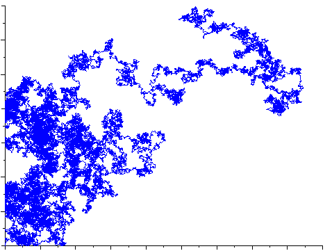
Figure 1: An example of path of reflected Brownian motion in the quadrant

1 Introduction and main results

Since its introduction in the eighties by Harrison, Reiman, Varadhan and Williams [31, 32, 55, 56, 57], reflected Brownian motion in the quarter plane has received a lot of attention from the probabilistic community. However, and surprisingly, finding a general explicit expression of the stationary distribution has been left as an open problem. The present paper solves this problem in a complete and unified way.

Reflected Brownian motion in two-dimensional cones

The semimartingale reflected Brownian motion with drift in the quarter plane +2:=[0,)2assignsuperscriptsubscript2superscript02\mathbb{R}_{+}^{2}:=[0,\infty)^{2} (or equivalently in arbitrary convex wedges, by performing a simple linear transformation, cf. Appendix A) can be written as

Z(t)=Z0+B(t)+μt+RL(t),t0,formulae-sequence𝑍𝑡subscript𝑍0𝐵𝑡𝜇𝑡𝑅𝐿𝑡for-all𝑡0Z(t)=Z_{0}+B(t)+\mu\cdot t+R\cdot L(t),\qquad\forall t\geqslant 0, (1)

where

  • Z0subscript𝑍0Z_{0} is any initial point in the quadrant,

  • B𝐵B is a Brownian motion with covariance Σ=(σ11σ12σ12σ22)Σsubscript𝜎11subscript𝜎12subscript𝜎12subscript𝜎22\Sigma=\small\left(\begin{array}[]{ll}\sigma_{11}&\sigma_{12}\\ \sigma_{12}&\sigma_{22}\end{array}\right) starting from the origin,

  • μ=(μ1μ2)𝜇subscript𝜇1subscript𝜇2\mu=\small\left(\begin{array}[]{l}\mu_{1}\\ \mu_{2}\end{array}\right) denotes the interior drift,

  • R=(R1,R2)=(r11r12r21r22)𝑅superscript𝑅1superscript𝑅2subscript𝑟11subscript𝑟12subscript𝑟21subscript𝑟22R=(R^{1},R^{2})=\small\left(\begin{array}[]{cc}r_{11}&r_{12}\\ r_{21}&r_{22}\end{array}\right) is the reflection matrix,

  • L=(L1L2)𝐿superscript𝐿1superscript𝐿2L=\small\left(\begin{array}[]{l}L^{1}\\ L^{2}\end{array}\right) is the local time.

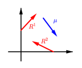
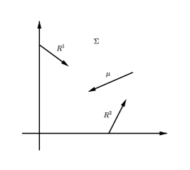
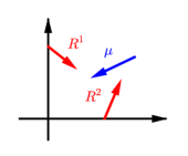
For i{1,2}𝑖12i\in\{1,2\}, the local time Li(t)superscript𝐿𝑖𝑡L^{i}(t) is a continuous non-decreasing process starting from 00 (i.e., Li(0)=0superscript𝐿𝑖00L^{i}(0)=0), increasing only at time t𝑡t such that Zi(t)=0superscript𝑍𝑖𝑡0Z^{i}(t)=0, viz., 0t𝟙{Zi(s)0}dLi(s)=0superscriptsubscript0𝑡subscript1superscript𝑍𝑖𝑠0differential-dsuperscript𝐿𝑖𝑠0\int_{0}^{t}\mathds{1}_{\{Z^{i}(s)\neq 0\}}\mathrm{d}L^{i}(s)=0, for all t0𝑡0t\geqslant 0. The columns R1superscript𝑅1R^{1} and R2superscript𝑅2R^{2} represent the directions in which the Brownian motion is pushed when the axes are reached, see Figure 2.

The reflected Brownian motion (Z(t))t0subscript𝑍𝑡𝑡0(Z(t))_{t\geqslant 0} associated with (Σ,μ,R)Σ𝜇𝑅(\Sigma,\mu,R) is well defined [55, 57], and is a fundamental stochastic process. This process has been extensively explored, and its multidimensional version (a semimartingale reflected Brownian motion in the positive orthant +dsuperscriptsubscript𝑑\mathbb{R}_{+}^{d}, as well as in convex polyhedrons) as well. It has been studied in depth, with focuses on its definition and semimartingale properties [55, 56, 16, 58], its recurrence or transience [56, 13, 35, 9, 7, 6, 15], the possible particular (e.g., product) form of its stationary distribution [34, 19, 47], its Lyapunov functions [23], its links with other stochastic processes [42, 22, 43], its use to approximate large queuing networks [26, 2, 33, 38, 37], the asymptotics of its stationary distribution [30, 17, 28, 49], numerical methods to compute the stationary distribution [13, 14], links with complex analysis [26, 2, 8, 29], comparison and coupling techniques [51, 50], etc.

The main contribution of the present paper is to find an exact expression for the stationary distribution (via its Laplace transforms, to be introduced in (3) and (4)), thanks to the theory of boundary value problems (BVPs), see our Theorem 1. This is one of the first attempts to apply boundary value techniques to diffusions in the quadrant, after [27] (under the symmetry conditions μ1=μ2subscript𝜇1subscript𝜇2\mu_{1}=\mu_{2}, σ11=σ22subscript𝜎11subscript𝜎22\sigma_{11}=\sigma_{22}, and symmetric reflection vectors in (1)), [26] (which concerns very specific cases of the covariance matrix, essentially the identity), [2] (on diffusions with a special behavior on the boundary), [29] (orthogonal reflections, solved by Tutte’s invariant approach [54, 3]); see also the introduction of [17], where the authors allude to the possibility of such an approach. The application of BVP techniques to discrete models has a longer history, see [25, 39, 3] and references therein.
Refer to caption
(a) μ1<0,μ2<0formulae-sequencesubscript𝜇10subscript𝜇20\mu_{1}<0,\ \mu_{2}<0
Refer to caption
(b) μ1<0,μ20formulae-sequencesubscript𝜇10subscript𝜇20\mu_{1}<0,\ \mu_{2}\geqslant 0
Refer to caption
(c) μ10,μ2<0formulae-sequencesubscript𝜇10subscript𝜇20\mu_{1}\geqslant 0,\ \mu_{2}<0
Figure 2: Drift μ𝜇\mu and reflection vectors R1superscript𝑅1R^{1} and R2superscript𝑅2R^{2}

Laplace transforms and functional equation

The reflected Brownian motion defined in (1) exists if and only if

{r11>0,r22>0,detR>0}or{r11>0,r22>0,r12>0,r21>0}.formulae-sequencesubscript𝑟110formulae-sequencesubscript𝑟220𝑅0orformulae-sequencesubscript𝑟110formulae-sequencesubscript𝑟220formulae-sequencesubscript𝑟120subscript𝑟210\{r_{11}>0,\quad r_{22}>0,\quad\det R>0\}\quad\text{or}\quad\{r_{11}>0,\quad r_{22}>0,\quad r_{12}>0,\quad r_{21}>0\}.

This condition is equivalent for R𝑅R to be completely-𝒮𝒮\mathcal{S}, which actually is a necessary and sufficient condition to the existence of reflected Brownian motion in arbitrary dimension, see [53, 48].

As for the stationary distribution, it exists if and only if

r11>0,r22>0,r11r22r12r21>0,r22μ1r12μ2<0,r11μ2r21μ1<0,formulae-sequencesubscript𝑟110formulae-sequencesubscript𝑟220formulae-sequencesubscript𝑟11subscript𝑟22subscript𝑟12subscript𝑟210formulae-sequencesubscript𝑟22subscript𝜇1subscript𝑟12subscript𝜇20subscript𝑟11subscript𝜇2subscript𝑟21subscript𝜇10r_{11}>0,\quad r_{22}>0,\quad r_{11}r_{22}-r_{12}r_{21}>0,\quad r_{22}\mu_{1}-r_{12}\mu_{2}<0,\quad r_{11}\mu_{2}-r_{21}\mu_{1}<0, (2)

see [33, 30], and in that case it is absolutely continuous w.r.t. the Lebesgue measure [13, 14, 33], with density denoted by π(x)=π(x1,x2)𝜋𝑥𝜋subscript𝑥1subscript𝑥2\pi(x)=\pi(x_{1},x_{2}). See Figure 2 for an example of parameters satisfying to (2); there are three different cases, according to the sign of the drift coordinates (having two non-negative coordinates is obviously incompatible with (2)). Assumption (2) implies in particular that R𝑅R is invertible and R1μ<0superscript𝑅1𝜇0R^{-1}\mu<0, which turns out to be a necessary condition for the existence of the stationary distribution in any dimension, see [33]. From now, we will assume that (2) is satisfied. Let the Laplace transform of π𝜋\pi be defined by

φ(θ)=𝔼π[exp(θZ)]=+2exp(θx)π(x)dx.𝜑𝜃subscript𝔼𝜋delimited-[]𝜃𝑍subscriptdouble-integralsuperscriptsubscript2𝜃𝑥𝜋𝑥differential-d𝑥\varphi(\theta)=\mathbb{E}_{\pi}[\exp{(\theta\cdot Z)}]=\iint_{{\mathbb{R}}_{+}^{2}}\exp{(\theta\cdot x)}\pi(x)\mathrm{d}x. (3)

Furthermore we define two finite boundary measures ν1subscript𝜈1\nu_{1} and ν2subscript𝜈2\nu_{2} such that, for A+𝐴subscriptA\subset\mathbb{R}_{+},

ν1(A)=𝔼π[01𝟙{Z(t){0}×A}dL1(t)],ν2(A)=𝔼π[01𝟙{Z(t)A×{0}}dL2(t)].formulae-sequencesubscript𝜈1𝐴subscript𝔼𝜋delimited-[]superscriptsubscript01subscript1𝑍𝑡0𝐴differential-dsuperscript𝐿1𝑡subscript𝜈2𝐴subscript𝔼𝜋delimited-[]superscriptsubscript01subscript1𝑍𝑡𝐴0differential-dsuperscript𝐿2𝑡\nu_{1}(A)=\mathbb{E}_{\pi}\bigg{[}\int_{0}^{1}\mathds{1}_{\{Z(t)\in\{0\}\times A\}}\mathrm{d}L^{1}(t)\bigg{]},\qquad\nu_{2}(A)=\mathbb{E}_{\pi}\bigg{[}\int_{0}^{1}\mathds{1}_{\{Z(t)\in A\times\{0\}\}}\mathrm{d}L^{2}(t)\bigg{]}.

The νisubscript𝜈𝑖\nu_{i} have their supports on the axes and may be viewed as boundary invariant measures. They are continuous w.r.t. the Lebesgue measure, see [34]. We define their Laplace transform by

φ1(θ2)=+exp(θ2x2)ν1(x2)dx2,φ2(θ1)=+exp(θ1x1)ν2(x1)dx1.formulae-sequencesubscript𝜑1subscript𝜃2subscriptsubscriptsubscript𝜃2subscript𝑥2subscript𝜈1subscript𝑥2differential-dsubscript𝑥2subscript𝜑2subscript𝜃1subscriptsubscriptsubscript𝜃1subscript𝑥1subscript𝜈2subscript𝑥1differential-dsubscript𝑥1\varphi_{1}(\theta_{2})=\int_{{\mathbb{R}}_{+}}\exp({\theta_{2}x_{2}})\nu_{1}(x_{2})\mathrm{d}x_{2},\qquad\varphi_{2}(\theta_{1})=\int_{{\mathbb{R}}_{+}}\exp({\theta_{1}x_{1}})\nu_{2}(x_{1})\mathrm{d}x_{1}. (4)

The following functional equation relates the Laplace transforms:

γ(θ)φ(θ)=γ1(θ)φ1(θ2)+γ2(θ)φ2(θ1),𝛾𝜃𝜑𝜃subscript𝛾1𝜃subscript𝜑1subscript𝜃2subscript𝛾2𝜃subscript𝜑2subscript𝜃1-\gamma(\theta)\varphi(\theta)=\gamma_{1}(\theta)\varphi_{1}(\theta_{2})+\gamma_{2}(\theta)\varphi_{2}(\theta_{1}), (5)

where we have noted

{γ(θ)=12(θΣθ)+θμ=12(σ11θ12+2σ12θ1θ2+σ22θ22)+μ1θ1+μ2θ2,γ1(θ)=R1θ=r11θ1+r21θ2,γ2(θ)=R2θ=r12θ1+r22θ2.cases𝛾𝜃12𝜃Σ𝜃𝜃𝜇12subscript𝜎11superscriptsubscript𝜃122subscript𝜎12subscript𝜃1subscript𝜃2subscript𝜎22superscriptsubscript𝜃22subscript𝜇1subscript𝜃1subscript𝜇2subscript𝜃2otherwisesubscript𝛾1𝜃superscript𝑅1𝜃subscript𝑟11subscript𝜃1subscript𝑟21subscript𝜃2otherwisesubscript𝛾2𝜃superscript𝑅2𝜃subscript𝑟12subscript𝜃1subscript𝑟22subscript𝜃2otherwise\begin{cases}\hskip 4.2679pt\gamma(\theta)=\frac{1}{2}{\color[rgb]{0,0,0}(\theta\cdot\Sigma\theta)+\theta\cdot\mu}=\frac{1}{2}(\sigma_{11}\theta_{1}^{2}+2\sigma_{12}\theta_{1}\theta_{2}+\sigma_{22}\theta_{2}^{2})+\mu_{1}\theta_{1}+\mu_{2}\theta_{2},\\ \gamma_{1}(\theta)={\color[rgb]{0,0,0}R^{1}\cdot\theta}=r_{11}\theta_{1}+r_{21}\theta_{2},\\ \gamma_{2}(\theta)={\color[rgb]{0,0,0}R^{2}\cdot\theta}=r_{12}\theta_{1}+r_{22}\theta_{2}.\end{cases} (6)

The Laplace transforms (3) and (4) (resp. Equation (5)) exist (resp. holds) at least for values of θ=(θ1,θ2)𝜃subscript𝜃1subscript𝜃2\theta=(\theta_{1},\theta_{2}) with θ10subscript𝜃10{\Re}\,\theta_{1}\leqslant 0 and θ20subscript𝜃20{\Re}\,\theta_{2}\leqslant 0. To prove the functional equation (5), the main idea is to use an identity called basic adjoint relationship (BAR); see [29, Section 2.1] and [17, 26] for details.

Kernel and associated quantities

In this paragraph we introduce necessary notation to state our main results. By definition, the kernel of (5) is the second degree polynomial γ𝛾\gamma. With this terminology, (5) is sometimes referred to as a kernel equation. The equality γ(θ1,θ2)=0𝛾subscript𝜃1subscript𝜃20\gamma(\theta_{1},\theta_{2})=0 with θ1,θ2subscript𝜃1subscript𝜃2\theta_{1},\theta_{2}\in\mathbb{C} defines algebraic functions Θ1±(θ2)superscriptsubscriptΘ1plus-or-minussubscript𝜃2\Theta_{1}^{\pm}(\theta_{2}) and Θ2±(θ1)superscriptsubscriptΘ2plus-or-minussubscript𝜃1\Theta_{2}^{\pm}(\theta_{1}) by

γ(Θ1±(θ2),θ2)=γ(θ1,Θ2±(θ1))=0.𝛾superscriptsubscriptΘ1plus-or-minussubscript𝜃2subscript𝜃2𝛾subscript𝜃1superscriptsubscriptΘ2plus-or-minussubscript𝜃10\gamma(\Theta_{1}^{\pm}(\theta_{2}),\theta_{2})=\gamma(\theta_{1},\Theta_{2}^{\pm}(\theta_{1}))=0.

Solving these equations readily yields

{Θ1±(θ2)=(σ12θ2+μ1)±θ22(σ122σ11σ22)+2θ2(μ1σ12μ2σ11)+μ12σ11,Θ2±(θ1)=(σ12θ1+μ2)±θ12(σ122σ11σ22)+2θ1(μ2σ12μ1σ22)+μ22σ22.casessuperscriptsubscriptΘ1plus-or-minussubscript𝜃2plus-or-minussubscript𝜎12subscript𝜃2subscript𝜇1superscriptsubscript𝜃22superscriptsubscript𝜎122subscript𝜎11subscript𝜎222subscript𝜃2subscript𝜇1subscript𝜎12subscript𝜇2subscript𝜎11superscriptsubscript𝜇12subscript𝜎11superscriptsubscriptΘ2plus-or-minussubscript𝜃1plus-or-minussubscript𝜎12subscript𝜃1subscript𝜇2superscriptsubscript𝜃12superscriptsubscript𝜎122subscript𝜎11subscript𝜎222subscript𝜃1subscript𝜇2subscript𝜎12subscript𝜇1subscript𝜎22superscriptsubscript𝜇22subscript𝜎22\left\{\begin{array}[]{l}\Theta_{1}^{\pm}(\theta_{2})=\dfrac{-(\sigma_{12}\theta_{2}+\mu_{1})\pm\sqrt{\theta_{2}^{2}(\sigma_{12}^{2}-\sigma_{11}\sigma_{22})+2\theta_{2}(\mu_{1}\sigma_{12}-\mu_{2}\sigma_{11})+\mu_{1}^{2}}}{\sigma_{11}},\vskip 3.0pt plus 1.0pt minus 1.0pt\vskip 3.0pt plus 1.0pt minus 1.0pt\\ \Theta_{2}^{\pm}(\theta_{1})=\dfrac{-(\sigma_{12}\theta_{1}+\mu_{2})\pm\sqrt{\theta_{1}^{2}(\sigma_{12}^{2}-\sigma_{11}\sigma_{22})+2\theta_{1}(\mu_{2}\sigma_{12}-\mu_{1}\sigma_{22})+\mu_{2}^{2}}}{\sigma_{22}}.\end{array}\right. (7)

The polynomials under the square roots in (7) have two zeros (called branch points), real and of opposite signs. They are denoted by θ2±superscriptsubscript𝜃2plus-or-minus\theta_{2}^{\pm} and θ1±superscriptsubscript𝜃1plus-or-minus\theta_{1}^{\pm}, respectively:

{θ2±=(μ1σ12μ2σ11)±(μ1σ12μ2σ11)2+μ12detΣdetΣ,θ1±=(μ2σ12μ1σ22)±(μ2σ12μ1σ22)2+μ22detΣdetΣ.casessuperscriptsubscript𝜃2plus-or-minusplus-or-minussubscript𝜇1subscript𝜎12subscript𝜇2subscript𝜎11superscriptsubscript𝜇1subscript𝜎12subscript𝜇2subscript𝜎112superscriptsubscript𝜇12ΣΣsuperscriptsubscript𝜃1plus-or-minusplus-or-minussubscript𝜇2subscript𝜎12subscript𝜇1subscript𝜎22superscriptsubscript𝜇2subscript𝜎12subscript𝜇1subscript𝜎222superscriptsubscript𝜇22ΣΣ\left\{\begin{array}[]{l}\displaystyle\theta_{2}^{\pm}=\frac{(\mu_{1}\sigma_{12}-\mu_{2}\sigma_{11})\pm\sqrt{(\mu_{1}\sigma_{12}-\mu_{2}\sigma_{11})^{2}+\mu_{1}^{2}\det{\Sigma}}}{\det\Sigma},\vskip 3.0pt plus 1.0pt minus 1.0pt\vskip 3.0pt plus 1.0pt minus 1.0pt\\ \displaystyle\theta_{1}^{\pm}=\frac{(\mu_{2}\sigma_{12}-\mu_{1}\sigma_{22})\pm\sqrt{(\mu_{2}\sigma_{12}-\mu_{1}\sigma_{22})^{2}+\mu_{2}^{2}\det{\Sigma}}}{\det\Sigma}.\end{array}\right. (8)

The algebraic functions Θ1±(θ2)superscriptsubscriptΘ1plus-or-minussubscript𝜃2\Theta_{1}^{\pm}(\theta_{2}) are meromorphic on the cut plane ((,θ2][θ2+,))superscriptsubscript𝜃2superscriptsubscript𝜃2\mathbb{C}\setminus((-\infty,\theta_{2}^{-}]\cup[\theta_{2}^{+},\infty)). Similarly, Θ2±(θ1)superscriptsubscriptΘ2plus-or-minussubscript𝜃1\Theta_{2}^{\pm}(\theta_{1}) are meromorphic on ((,θ1][θ1+,))superscriptsubscript𝜃1superscriptsubscript𝜃1\mathbb{C}\setminus((-\infty,\theta_{1}^{-}]\cup[\theta_{1}^{+},\infty)).

Our next important definition is the curve

={θ2:γ(θ1,θ2)=0 and θ1(,θ1)}.conditional-setsubscript𝜃2𝛾subscript𝜃1subscript𝜃20 and subscript𝜃1superscriptsubscript𝜃1\mathcal{R}=\{\theta_{2}\in\mathbb{C}:\gamma(\theta_{1},\theta_{2})=0\text{ and }\theta_{1}\in(-\infty,\theta_{1}^{-})\}.

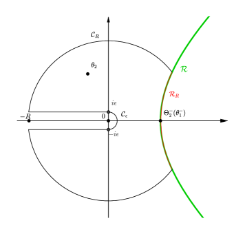
As it will be seen in Lemma 4 (see also Figure 7), \mathcal{R} is a branch of hyperbola. We denote by

={θ2:θ20}superscriptconditional-setsubscript𝜃2subscript𝜃20\mathcal{R}^{-}=\{\theta_{2}\in\mathcal{R}:\Im\,\theta_{2}\leqslant 0\} (9)

the negative imaginary part of \mathcal{R} oriented from the vertex to infinity.

We further define the function

w(θ2)=Tπβ(2θ2(θ2++θ2)θ2+θ2),𝑤subscript𝜃2subscript𝑇𝜋𝛽2subscript𝜃2superscriptsubscript𝜃2superscriptsubscript𝜃2superscriptsubscript𝜃2superscriptsubscript𝜃2w(\theta_{2})=T_{\frac{\pi}{\beta}}\left(-\frac{2\theta_{2}-(\theta_{2}^{+}+\theta_{2}^{-})}{\theta_{2}^{+}-\theta_{2}^{-}}\right), (10)

where

β=arccosσ12σ11σ22𝛽subscript𝜎12subscript𝜎11subscript𝜎22\beta=\arccos{-\frac{\sigma_{12}}{\sqrt{\sigma_{11}\sigma_{22}}}} (11)

and for a0𝑎0a\geqslant 0, Tasubscript𝑇𝑎T_{a} is the so-called generalized Chebyshev polynomial

Ta(x)=cos(aarccosx)=12{(x+x21)a+(xx21)a}.subscript𝑇𝑎𝑥𝑎𝑥12superscript𝑥superscript𝑥21𝑎superscript𝑥superscript𝑥21𝑎T_{a}(x)=\cos(a\arccos x)=\frac{1}{2}\Big{\{}\big{(}x+\sqrt{x^{2}-1}\big{)}^{a}+\big{(}x-\sqrt{x^{2}-1}\big{)}^{a}\Big{\}}. (12)

The function w𝑤w plays a special role regarding the curve \mathcal{R}, as for θ2subscript𝜃2\theta_{2}\in\mathcal{R} it satisfies w(θ2)=w(θ2¯)𝑤subscript𝜃2𝑤¯subscript𝜃2w(\theta_{2})=w(\overline{\theta_{2}}), see Lemma 9. (Here and throughout, θ2¯¯subscript𝜃2\overline{\theta_{2}} denotes the complex conjugate number of θ2subscript𝜃2\theta_{2}.)

Finally, let G𝐺G be the function whose expression is

G(θ2)=γ1γ2(Θ1(θ2),θ2)γ2γ1(Θ1(θ2¯),θ2¯).𝐺subscript𝜃2subscript𝛾1subscript𝛾2superscriptsubscriptΘ1subscript𝜃2subscript𝜃2subscript𝛾2subscript𝛾1superscriptsubscriptΘ1¯subscript𝜃2¯subscript𝜃2G(\theta_{2})=\frac{\gamma_{1}}{\gamma_{2}}(\Theta_{1}^{-}(\theta_{2}),\theta_{2})\frac{\gamma_{2}}{\gamma_{1}}(\Theta_{1}^{-}(\overline{\theta_{2}}),\overline{\theta_{2}}). (13)

Main results

Our main result can be stated as follows.

Theorem 1.

Under the assumption (2), the Laplace transform φ1subscript𝜑1\varphi_{1} in (4) is equal to

φ1(θ2)=ν1(+)(w(0)w(p)w(θ2)w(p))χexp{12iπlogG(θ)[w(θ)w(θ)w(θ2)w(θ)w(θ)w(0)]dθ},subscript𝜑1subscript𝜃2subscript𝜈1subscriptsuperscript𝑤0𝑤𝑝𝑤subscript𝜃2𝑤𝑝𝜒12𝑖𝜋subscriptsuperscript𝐺𝜃delimited-[]superscript𝑤𝜃𝑤𝜃𝑤subscript𝜃2superscript𝑤𝜃𝑤𝜃𝑤0differential-d𝜃\varphi_{1}(\theta_{2})=\\ \nu_{1}(\mathbb{R}_{+})\left(\frac{w(0)-w(p)}{w(\theta_{2})-w(p)}\right)^{-\chi}\exp\bigg{\{}\frac{1}{2i\pi}\int_{\mathcal{R}^{-}}\log G(\theta)\left[\frac{w^{\prime}(\theta)}{w(\theta)-w(\theta_{2})}-\frac{w^{\prime}(\theta)}{w(\theta)-w(0)}\right]\mathrm{d}\theta\bigg{\}}, (14)

where

  • w𝑤w, G𝐺G and superscript\mathcal{R}^{-} are defined in (10), (13) and (9), respectively,

  • ν1(+)=r12μ2r22μ1detRsubscript𝜈1subscriptsubscript𝑟12subscript𝜇2subscript𝑟22subscript𝜇1𝑅\displaystyle\nu_{1}(\mathbb{R}_{+})=\frac{r_{12}\mu_{2}-r_{22}\mu_{1}}{\det R},

  • the index χ𝜒\chi is given by χ={0if γ1(θ1,Θ2(θ1))0,1if γ1(θ1,Θ2(θ1))>0,𝜒cases0if subscript𝛾1superscriptsubscript𝜃1superscriptsubscriptΘ2superscriptsubscript𝜃101if subscript𝛾1superscriptsubscript𝜃1superscriptsubscriptΘ2superscriptsubscript𝜃10\chi=\left\{\begin{array}[]{rl}0&\displaystyle\text{if }\gamma_{1}(\theta_{1}^{-},\Theta_{2}^{-}(\theta_{1}^{-}))\leqslant 0,\vskip 3.0pt plus 1.0pt minus 1.0pt\\ -1&\displaystyle\text{if }\gamma_{1}(\theta_{1}^{-},\Theta_{2}^{-}(\theta_{1}^{-}))>0,\end{array}\right.

  • p=2r11(μ1r21μ2r11)r112σ222r11r21σ12+r212σ11𝑝2subscript𝑟11subscript𝜇1subscript𝑟21subscript𝜇2subscript𝑟11superscriptsubscript𝑟112subscript𝜎222subscript𝑟11subscript𝑟21subscript𝜎12superscriptsubscript𝑟212subscript𝜎11\displaystyle p=\frac{2r_{11}(\mu_{1}r_{21}-\mu_{2}r_{11})}{r_{11}^{2}\sigma_{22}-2r_{11}r_{21}\sigma_{12}+r_{21}^{2}\sigma_{11}},

  • to define the function logG(θ)𝐺𝜃\log G(\theta) on superscript\mathcal{R}^{-}, we use the determination of the logarithm taking a value in i(π,π]𝑖𝜋𝜋i\cdot(-\pi,\pi] at the vertex of superscript\mathcal{R}^{-} and varying continuously over the curve superscript\mathcal{R}^{-}.

The function φ2(θ1)subscript𝜑2subscript𝜃1\varphi_{2}(\theta_{1}) equals φ1(θ1)subscript𝜑1subscript𝜃1\varphi_{1}(\theta_{1}) in (14) after the change of parameters

σ11σ22,μ1μ2,r11r22,r12r21.subscript𝜎11subscript𝜎22subscript𝜇1subscript𝜇2subscript𝑟11subscript𝑟22subscript𝑟12subscript𝑟21\sigma_{11}\leftrightarrow\sigma_{22},\quad\mu_{1}\leftrightarrow\mu_{2},\quad r_{11}\leftrightarrow r_{22},\quad r_{12}\leftrightarrow r_{21}.

The functional equation (5) finally gives an explicit formula for the bivariate Laplace transform φ𝜑\varphi.

Let us now give some comments around Theorem 1.

  • Theorem 1 completely generalizes the results of [27] (with symmetry conditions), [26] (with the identity covariance matrix ΣΣ\Sigma) and [29] (orthogonal reflections on the axes). It offers the first explicit expression of the Laplace transforms, covering all the range of parameters (Σ,μ,R)Σ𝜇𝑅(\Sigma,\mu,R) satisfying to (2), thereby solving an old open problem.

  • We obtain three corollaries of Theorem 1, each of those corresponds to an already known result: we first compute the asymptotics of the boundary densities (Section 4.1, initially obtained in [18]); second we derive the product form expression of the density in the famous skew-symmetric case (Section 5.2, result originally proved in [34]); finally we compute the expression of the Laplace transforms in the case of orthogonal reflections (Section 5.4, see [29] for the first derivation).

  • It is worth remarking that the expression (14) is intrinsically non-continuous in terms of the parameters: the index χ𝜒\chi can indeed take two different values (namely, 00 and 111). For this reason, (14) actually contains two different formulas. See Remarks 7 and 18 for further related comments.

  • The paper [28] obtains the exact asymptotics of the stationary distribution along any direction in the quarter plane, see [28, Theorems 22–28]. Constants in these asymptotics involve the functions φ1subscript𝜑1\varphi_{1} and φ2subscript𝜑2\varphi_{2} in (4), and can thus be made explicit with Theorem 1.

  • It is also interesting to dissect (14) and to notice that certain quantities in that formula depend only on the behavior of the process in the interior of the quadrant (w𝑤w and superscript\mathcal{R}^{-}), while the remaining ones mix properties of the interior and boundary of the quarter plane (ν1(+)subscript𝜈1subscript\nu_{1}(\mathbb{R}_{+}), p𝑝p, χ𝜒\chi and G𝐺G).

  • The statement of Theorem 1 (namely, an expression of the Laplace transform as a Cauchy integral), as well as the techniques we shall employ to prove it (viz., reduction to BVPs with shift), are reminiscent of the results and methods used for discrete random walks in the quarter plane, see [25] for a modern reference, and [45, 24, 39] for historical breakthroughs.

  • Altogether, Theorem 1 illustrates that the analytic approach consisting in solving quarter plane problems via BVPs is better suited for diffusions than for discrete random walks. We can actually treat any wedge, covariance matrix, drift vector and reflection vectors (see Corollary 2 below), whereas in the discrete case, hypotheses should be done on the boundedness of the jumps (only small steps are considered in [25, 39, 5, 3]) and on the cone (typically, half and quarter planes only).

Theorem 1 further leads to an explicit expression for the Laplace transform of the stationary distribution of reflected Brownian motion in an arbitrary convex wedge, as stated in the following corollary, whose proof is postponed to Appendix A.

Corollary 2.

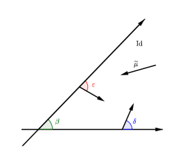
Let Z~~𝑍\widetilde{Z} be a reflected Brownian motion in a wedge of angle β(0,π)𝛽0𝜋\beta\in(0,\pi), of covariance matrix Σ~~Σ\widetilde{\Sigma}, drift μ~~𝜇\widetilde{\mu} and reflection matrix R~=(R~1,R~2)~𝑅superscript~𝑅1superscript~𝑅2\widetilde{R}=(\widetilde{R}^{1},\widetilde{R}^{2}), corresponding to the angles of reflection δ𝛿\delta and ε𝜀\varepsilon on Figure 13. Assume it is recurrent and note π~~𝜋\widetilde{\pi} the stationary distribution and φ~~𝜑\widetilde{\varphi} its Laplace transform. Let

T1=(1sinβcotβ01),T11=(sinβcosβ01).formulae-sequencesubscript𝑇1matrix1𝛽𝛽01superscriptsubscript𝑇11matrix𝛽𝛽01T_{1}=\begin{pmatrix}\frac{1}{\sin\beta}&\cot\beta\\ 0&1\end{pmatrix},\qquad T_{1}^{-1}=\begin{pmatrix}\sin\beta&-{\cos\beta}\\ 0&\phantom{-}1\end{pmatrix}.

Then

φ~(θ~)=φ(T1θ~),~𝜑~𝜃𝜑superscriptsubscript𝑇1top~𝜃\widetilde{\varphi}(\widetilde{\theta})=\varphi(T_{1}^{\top}\widetilde{\theta}),

where φ𝜑\varphi is the Laplace transform (14) of Theorem 1 associated to (Σ,μ,R)Σ𝜇𝑅(\Sigma,\mu,R), with

Σ=T1Σ~T1,μ=T11μ~andR=T11R~.formulae-sequenceΣsubscript𝑇1~Σsuperscriptsubscript𝑇1topformulae-sequence𝜇superscriptsubscript𝑇11~𝜇and𝑅superscriptsubscript𝑇11~𝑅\Sigma=T_{1}\widetilde{\Sigma}T_{1}^{\top},\quad\mu=T_{1}^{-1}\widetilde{\mu}\quad\text{and}\quad R=T_{1}^{-1}\widetilde{R}.

Structure of the paper

  • Section 2: analytic preliminaries, continuation of the Laplace transforms and definition of an important hyperbola

  • Section 3: statement and proof that the Laplace transforms satisfy BVP of Carleman-type on branches of hyperbolas, transformation of the Carleman BVP with shift into a (more classical) Riemann BVP, study of the conformal mapping allowing this transformation, resolution of the BVP

  • Section 4: asymptotics of the stationary distribution, links with Dai and Miyazawa’s [18] asymptotic results

  • Section 5: simplifications of the integral expression of Theorem 1 for models satisfying the skew-symmetric condition, for orthogonal reflections (leading to a new proof of the results of [29]), links with Dieker and Moriarty’s results [19]

  • Appendix A: equivalence between Brownian motion in the quarter plane and Brownian motion in convex wedges

Acknowledgements

We thank Irina Kurkova and Yuri Suhov for interesting discussions. We acknowledge support from the “projet MADACA” (2014–2016), funded by the Région Centre-Val de Loire (France). Finally we thank the editors and referees for their useful remarks and suggestions.

2 Methodology and analytic preliminaries

2.1 Methodology and positioning of our work regarding [27, 26, 2, 17]

Schematically, our argument for the proof of Theorem 1 is composed of the following steps:

  1. (1)

    presentation of the functional equation, analytic preliminaries, meromorphic continuation of the Laplace transforms (Section 2);

  2. (2)

    statement of a Carleman BVP with shift satisfied by the Laplace transforms (Section 3.1);

  3. (3)

    introduction of a conformal mapping, allowing to transform the latter BVP into a more classical Riemann BVP (Section 3.2), see Figure 8;

  4. (4)

    statement of the Riemann BVP (Section 3.3);

  5. (5)

    definition and study of the index (denoted by χ𝜒\chi in Theorem 1), which turns out to have a crucial role in solving the Riemann BVP (Section 3.4);

  6. (6)

    resolution of the BVP (Section 3.5).

Except for the study of the index (item (5), which is specific to our problem at hand), the above structuration of the proof dates back to (in chronological order) [24] (for the discrete setting, which later led to the book [25]), [27], [26] and [2].

To begin the discussion, let us remind that the process in [2] is absorbed on the boundary and then relaunched in the quadrant after an exponential time; it is therefore totally different from ours. Let us also recall that the analytic study of reflected Brownian motion in the quadrant was initiated in [27, 26], but both [27] and [26] did quite restrictive assumptions on the process (symmetry conditions μ1=μ2subscript𝜇1subscript𝜇2\mu_{1}=\mu_{2}, σ11=σ22subscript𝜎11subscript𝜎22\sigma_{11}=\sigma_{22}, and symmetric reflection vectors in [27], identity covariance matrix in [26]).

In this paper we follow the same steps (1)(6) and use a synthetic approach of [24, 27, 26, 2], to eventually go further than the existing literature and prove Theorem 1. Some technical details of the present work are borrowed from [27, 26, 2] and more particularly from [2]. Although being different, the stochastic process of [2] and ours share the property of satisfying a functional equation with the same left-hand side (as in (5)). Accordingly, technical details will be very similar as soon as they concern the kernel; this is the case of Section 2. In particular, as in [2], the Laplace transforms will satisfy BVP on hyperbolas.

On the other hand, many points of our analysis profoundly differ from that of [2]: the resolution of the BVP is different as the right-hand side of (5) is not comparable to that of [2]. Moreover we make our main result as tractable as possible: see our Section 5, where we present many techniques to simplify the analytic expression derived in Theorem 1. We further also propose asymptotic considerations, in close relation to those of [17].

We shall prove in full detail our main results only in the case where both coordinates of the drift are negative:

μ1<0,μ2<0.formulae-sequencesubscript𝜇10subscript𝜇20\mu_{1}<0,\qquad\mu_{2}<0. (15)

This hypothesis (also done in [27, 26, 28]) is only technical, and allows us to reduce the number of cases to handle. In Section 3.6 we comment on the case of a drift μ𝜇\mu with one non-negative coordinate (having two non-negative coordinates is incompatible with (2)), and we explain how Theorem 1 remains valid in this case.

2.2 Real points of the kernel

The set of real points of the zero set of the kernel

{(θ1,θ2)2:γ(θ1,θ2)=0}conditional-setsubscript𝜃1subscript𝜃2superscript2𝛾subscript𝜃1subscript𝜃20\{(\theta_{1},\theta_{2})\in\mathbb{R}^{2}:\gamma(\theta_{1},\theta_{2})=0\}

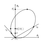
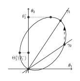
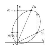
defines an ellipse, see Figure 3. Introduced in [17], this ellipse offers the possibility of presenting many analytical quantities in a clear and compact way:

  • the branch points θ1superscriptsubscript𝜃1\theta_{1}^{-} and θ1+superscriptsubscript𝜃1\theta_{1}^{+} (resp. θ2superscriptsubscript𝜃2\theta_{2}^{-} and θ2+superscriptsubscript𝜃2\theta_{2}^{+}) in (8) are the leftmost and rightmost (resp. bottommost and topmost) points on the ellipse;

  • the drift μ𝜇\mu is orthogonal to the tangent at the origin;

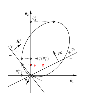
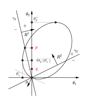
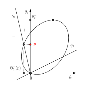
  • the set of points where γ1(θ1,θ2)=0subscript𝛾1subscript𝜃1subscript𝜃20\gamma_{1}(\theta_{1},\theta_{2})=0 and γ2(θ1,θ2)=0subscript𝛾2subscript𝜃1subscript𝜃20\gamma_{2}(\theta_{1},\theta_{2})=0 are straight lines, orthogonal to the reflection vectors R1superscript𝑅1R^{1} and R2superscript𝑅2R^{2}. Their intersection points with the ellipse are easily computed (notice that these intersection points appear in the statement of Theorem 1, in particular in the index χ𝜒\chi).

Refer to caption
Refer to caption
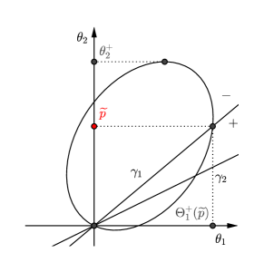
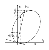
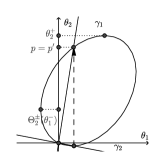
Figure 3: The ellipse and the two straight lines are the sets of real points (θ1,θ2)subscript𝜃1subscript𝜃2(\theta_{1},\theta_{2}) which cancel γ𝛾\gamma, γ1subscript𝛾1\gamma_{1} and γ2subscript𝛾2\gamma_{2}, respectively. Location of p𝑝p (see (18)) and q𝑞q (see (25)) according to the sign of γ1(θ1,Θ2(θ1))subscript𝛾1superscriptsubscript𝜃1superscriptsubscriptΘ2superscriptsubscript𝜃1\gamma_{1}(\theta_{1}^{-},\Theta_{2}^{-}(\theta_{1}^{-}))

2.3 Meromorphic continuation and poles of the Laplace transforms

In Section 3.1 we shall state a boundary condition for φ1subscript𝜑1\varphi_{1}, on a curve lying outside its natural domain of definition (namely, the half plane with negative real part). The statement hereafter (straightforward consequence of the functional equation (5), see Proposition 17 for an extended version) proposes a meromorphic continuation on a domain containing the latter curve.

Lemma 3.

The Laplace transform φ1(θ2)subscript𝜑1subscript𝜃2\varphi_{1}(\theta_{2}) can be extended meromorphically to the open and simply connected set

{θ2(θ2+,):θ20 or Θ1(θ2)<0},conditional-setsubscript𝜃2superscriptsubscript𝜃2subscript𝜃20 or superscriptsubscriptΘ1subscript𝜃20\{\theta_{2}\in{\color[rgb]{0,0,0}\mathbb{C}\setminus(\theta_{2}^{+},\infty)}:\Re\,\theta_{2}\leqslant 0\text{ or }\Re\,\Theta_{1}^{-}(\theta_{2})<0\}, (16)

by mean of the formula

φ1(θ2)=γ2γ1(Θ1(θ2),θ2)φ2(Θ1(θ2)).subscript𝜑1subscript𝜃2subscript𝛾2subscript𝛾1superscriptsubscriptΘ1subscript𝜃2subscript𝜃2subscript𝜑2superscriptsubscriptΘ1subscript𝜃2\varphi_{1}(\theta_{2})=-\frac{\gamma_{2}}{\gamma_{1}}(\Theta_{1}^{-}(\theta_{2}),\theta_{2})\varphi_{2}(\Theta_{1}^{-}(\theta_{2})). (17)
Proof.

The domain (16) is simply connected by [28, §2.4]. The formula (17), see [28, Lemma 6], is a direct consequence of the functional equation (5) evaluated at (Θ1(θ2),θ2)superscriptsubscriptΘ1subscript𝜃2subscript𝜃2(\Theta_{1}^{-}(\theta_{2}),\theta_{2}), first on the (non-empty) open domain

{θ2:θ2<0 and Θ1(θ2)<0}.conditional-setsubscript𝜃2subscript𝜃20 and superscriptsubscriptΘ1subscript𝜃20\{\theta_{2}\in\mathbb{C}:\Re\,\theta_{2}<0\text{ and }\Re\,\Theta_{1}^{-}(\theta_{2})<0\}.\qed

Due to the continuation formula (17), the only possible pole of φ1subscript𝜑1\varphi_{1} in the domain (16) will come from a cancelation of the denominator γ1subscript𝛾1\gamma_{1}. More precisely, let p𝑝p be the (unique, when it exists) non-zero point such that

γ1(Θ1(p),p)=0.subscript𝛾1superscriptsubscriptΘ1𝑝𝑝0\gamma_{1}(\Theta_{1}^{-}(p),p)=0. (18)

It follows from (18) that p𝑝p satisfies a second degree polynomial equation with real coefficients. As one of the roots is 00 the other one must be p𝑝p, which is then real and equals (when it exists)

p=2r11(μ1r21μ2r11)r112σ222r11r21σ12+r212σ11.𝑝2subscript𝑟11subscript𝜇1subscript𝑟21subscript𝜇2subscript𝑟11superscriptsubscript𝑟112subscript𝜎222subscript𝑟11subscript𝑟21subscript𝜎12superscriptsubscript𝑟212subscript𝜎11p=\frac{2r_{11}(\mu_{1}r_{21}-\mu_{2}r_{11})}{r_{11}^{2}\sigma_{22}-2r_{11}r_{21}\sigma_{12}+r_{21}^{2}\sigma_{11}}. (19)

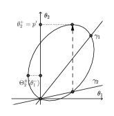
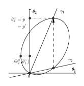
Formula (18) means that p𝑝p is the ordinate of the intersection point between the ellipse γ=0𝛾0\gamma=0 and the line γ1=0subscript𝛾10\gamma_{1}=0, see Figure 3. The intersection point always exists but sometimes its abscissa is associated to Θ1superscriptsubscriptΘ1\Theta_{1}^{-} (when p𝑝p exists, i.e., γ1(Θ1±(θ2+),θ2+)0subscript𝛾1superscriptsubscriptΘ1plus-or-minussuperscriptsubscript𝜃2superscriptsubscript𝜃20\gamma_{1}(\Theta_{1}^{\pm}(\theta_{2}^{+}),\theta_{2}^{+})\geqslant 0) and sometimes to Θ1+superscriptsubscriptΘ1\Theta_{1}^{+} (when p𝑝p doesn’t exist, i.e., γ1(Θ1±(θ2+),θ2+)<0subscript𝛾1superscriptsubscriptΘ1plus-or-minussuperscriptsubscript𝜃2superscriptsubscript𝜃20\gamma_{1}(\Theta_{1}^{\pm}(\theta_{2}^{+}),\theta_{2}^{+})<0), the limit case being p=θ2+𝑝superscriptsubscript𝜃2p=\theta_{2}^{+}, see Figure 4.

Refer to caption
Refer to caption
Figure 4: The intersection point between the ellipse γ=0𝛾0\gamma=0 and the straight line γ1=0subscript𝛾10\gamma_{1}=0. On the left side p𝑝p exists. On the right side p𝑝p doesn’t exist, although p~~𝑝\widetilde{p}, defined by that γ1(Θ1+(p~),p~)=0subscript𝛾1superscriptsubscriptΘ1~𝑝~𝑝0\gamma_{1}(\Theta_{1}^{+}(\widetilde{p}),\widetilde{p})=0, exists

Let us finally remark that the pole that φ1subscript𝜑1\varphi_{1} may have at p𝑝p is necessarily simple, due to the expression (6) of γ1subscript𝛾1\gamma_{1}.

2.4 An important hyperbola

For further use, we need to introduce the curve

={θ2:γ(θ1,θ2)=0 and θ1(,θ1)}=Θ2±((,θ1)).conditional-setsubscript𝜃2𝛾subscript𝜃1subscript𝜃20 and subscript𝜃1superscriptsubscript𝜃1superscriptsubscriptΘ2plus-or-minussuperscriptsubscript𝜃1\mathcal{R}=\{\theta_{2}\in\mathbb{C}:\gamma(\theta_{1},\theta_{2})=0\text{ and }\theta_{1}\in(-\infty,\theta_{1}^{-})\}=\Theta_{2}^{\pm}((-\infty,\theta_{1}^{-})). (20)

It is symmetrical w.r.t. the horizontal axis, see Figure 7. Indeed, the discriminant of Θ2±superscriptsubscriptΘ2plus-or-minus\Theta_{2}^{\pm} (i.e., the polynomial under the square root in (7)) is positive on (θ1,θ1+)superscriptsubscript𝜃1superscriptsubscript𝜃1(\theta_{1}^{-},\theta_{1}^{+}) and negative on [θ1,θ1+]superscriptsubscript𝜃1superscriptsubscript𝜃1{\mathbb{R}}\setminus[\theta_{1}^{-},\theta_{1}^{+}]. Accordingly, the branches Θ2±superscriptsubscriptΘ2plus-or-minus\Theta_{2}^{\pm} take respectively real and complex conjugate values on the sets above. Furthermore, \mathcal{R} has a simple structure, as shown by the following elementary result:

Lemma 4 (Lemma 9 in [2]).

The curve \mathcal{R} in (20) is a branch of hyperbola, whose equation is

σ22(σ122σ11σ22)x2+σ122σ22y22σ22(σ11μ2σ12μ1)x=μ2(σ11μ22σ12μ1).subscript𝜎22superscriptsubscript𝜎122subscript𝜎11subscript𝜎22superscript𝑥2superscriptsubscript𝜎122subscript𝜎22superscript𝑦22subscript𝜎22subscript𝜎11subscript𝜇2subscript𝜎12subscript𝜇1𝑥subscript𝜇2subscript𝜎11subscript𝜇22subscript𝜎12subscript𝜇1\sigma_{22}(\sigma_{12}^{2}-\sigma_{11}\sigma_{22})x^{2}+\sigma_{12}^{2}\sigma_{22}y^{2}-2\sigma_{22}(\sigma_{11}\mu_{2}-\sigma_{12}\mu_{1})x=\mu_{2}(\sigma_{11}\mu_{2}-2\sigma_{12}\mu_{1}). (21)

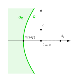
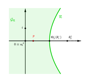
The curve \mathcal{R} is the right branch of the hyperbola if the covariance factor σ12>0subscript𝜎120\sigma_{12}>0, the left branch if σ12<0subscript𝜎120\sigma_{12}<0, and a vertical straight line in the limit case σ12=0subscript𝜎120\sigma_{12}=0.

Refer to caption
(a) σ12>0subscript𝜎120\sigma_{12}>0
Refer to caption
(b) σ12=0subscript𝜎120\sigma_{12}=0
Refer to caption
(c) σ12<0subscript𝜎120\sigma_{12}<0
Figure 5: The shape (in particular the orientation) of the curve \mathcal{R} depends directly on the sign of the covariance σ12subscript𝜎12\sigma_{12}

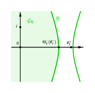
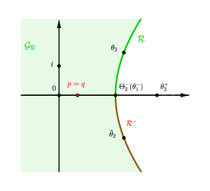
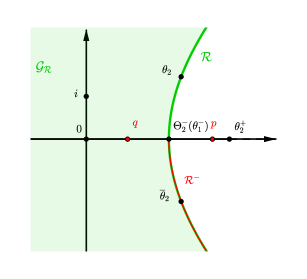
We denote the part of \mathcal{R} with negative imaginary part by superscript\mathcal{R}^{-}, see (9) and Figure 7. We further denote by 𝒢subscript𝒢\mathcal{G}_{\mathcal{R}} the open domain of \mathbb{C} containing 00 and bounded by \mathcal{R}, see again Figure 7. The closure of 𝒢subscript𝒢\mathcal{G}_{\mathcal{R}} is equal to 𝒢subscript𝒢\mathcal{G}_{\mathcal{R}}\cup\mathcal{R} and will be noted 𝒢¯¯subscript𝒢\overline{\mathcal{G}_{\mathcal{R}}}.

Lemma 5.

The domain

{θ2(θ2+,):θ20 or Θ1(θ2)<0},conditional-setsubscript𝜃2superscriptsubscript𝜃2subscript𝜃20 or superscriptsubscriptΘ1subscript𝜃20\{\theta_{2}\in\mathbb{C}\setminus(\theta_{2}^{+},\infty):\Re\,\theta_{2}\leqslant 0\text{ or }\Re\,\Theta_{1}^{-}(\theta_{2})<0\},

defined in (16), strictly contains 𝒢¯¯subscript𝒢\overline{\mathcal{G}_{\mathcal{R}}}.

Thanks to Lemma 3, this implies that the Laplace transform φ1(θ2)subscript𝜑1subscript𝜃2\varphi_{1}(\theta_{2}) can be extended meromorphically to a domain containing 𝒢¯¯subscript𝒢\overline{\mathcal{G}_{\mathcal{R}}}.

Proof.

The first way to see the above inclusion is to refer to [28], where the boundaries of the domain (16) (called Δ{s0}Δsubscript𝑠0\Delta\cup\{s_{0}\} in [28]) are computed, see in particular [28, Figures 10 and 11]. The technique used in [28] is to use the parametrization of the zero set of the kernel (6).

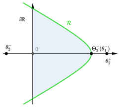
It is also possible to show it directly and more elementarily, as follows. First of all, the set 𝒢¯{θ2:θ20}¯subscript𝒢conditional-setsubscript𝜃2subscript𝜃20\overline{\mathcal{G}_{\mathcal{R}}}\cap\{\theta_{2}\in\mathbb{C}:\Re\,\theta_{2}\leqslant 0\} is obviously included in the domain defined in (16). It thus remains to show that the set 𝒢¯{θ2:θ2>0}¯subscript𝒢conditional-setsubscript𝜃2subscript𝜃20\overline{\mathcal{G}_{\mathcal{R}}}\cap\{\theta_{2}\in\mathbb{C}:\Re\,\theta_{2}>0\}, which is bounded by (a part of) \mathcal{R} and (a part of) i𝑖i\mathbb{R}, see Figure 6, is included in the domain (16). More specifically, we are going to prove that the latter set is a subset of

{θ2(θ2+,):Θ1(θ2)<0}.conditional-setsubscript𝜃2superscriptsubscript𝜃2superscriptsubscriptΘ1subscript𝜃20\{\theta_{2}\in\mathbb{C}\setminus(\theta_{2}^{+},\infty):\Re\,\Theta_{1}^{-}(\theta_{2})<0\}.

First, the definition (20) of \mathcal{R} obviously implies that {θ2(θ2+,):Θ1(θ2)<0}conditional-setsubscript𝜃2superscriptsubscript𝜃2superscriptsubscriptΘ1subscript𝜃20\mathcal{R}\subset\{\theta_{2}\in\mathbb{C}\setminus(\theta_{2}^{+},\infty):\Re\,\Theta_{1}^{-}(\theta_{2})<0\}. In the same way, we notice that i𝑖i\mathbb{R} also belongs to that set. Indeed, for t𝑡t\in\mathbb{R}, Equation (7) yields

Θ1(it)=1σ11(μ1μ12+t2detΣ+2it(μ1σ12μ2σ11))<0,superscriptsubscriptΘ1𝑖𝑡1subscript𝜎11subscript𝜇1superscriptsubscript𝜇12superscript𝑡2Σ2𝑖𝑡subscript𝜇1subscript𝜎12subscript𝜇2subscript𝜎110\Re\Theta_{1}^{-}(it)=\frac{1}{\sigma_{11}}\left(-\mu_{1}-\Re\sqrt{\mu_{1}^{2}+t^{2}\det\Sigma+2it(\mu_{1}\sigma_{12}-\mu_{2}\sigma_{11})}\right)<0,

because μ1<0subscript𝜇10\mu_{1}<0 by (15), and since ΣΣ\Sigma is a covariance matrix, detΣ>0Σ0\det\Sigma>0 and σ11>0subscript𝜎110\sigma_{11}>0. Then there are two cases to consider:

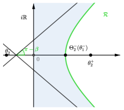
  • σ12<0subscript𝜎120\sigma_{12}<0 (i.e., 0<β<π20𝛽𝜋20<\beta<\frac{\pi}{2}): the set 𝒢¯{θ2:θ2>0}¯subscript𝒢conditional-setsubscript𝜃2subscript𝜃20\overline{\mathcal{G}_{\mathcal{R}}}\cap\{\theta_{2}\in\mathbb{C}:\Re\,\theta_{2}>0\} is bounded, see the left picture on Figure 6. Then the maximum principle applied to the function Θ1superscriptsubscriptΘ1\Re\Theta_{1}^{-} implies that the image of every point of the set 𝒢¯{θ2:θ2>0}¯subscript𝒢conditional-setsubscript𝜃2subscript𝜃20\overline{\mathcal{G}_{\mathcal{R}}}\cap\{\theta_{2}\in\mathbb{C}:\Re\,\theta_{2}>0\} by Θ1superscriptsubscriptΘ1\Re\Theta_{1}^{-} is negative.

  • σ120subscript𝜎120\sigma_{12}\geqslant 0 (i.e., π2β<π𝜋2𝛽𝜋\frac{\pi}{2}\leqslant\beta<\pi): it is no more possible to apply directly the maximum principle, as the set 𝒢¯{θ2:θ2>0}¯subscript𝒢conditional-setsubscript𝜃2subscript𝜃20\overline{\mathcal{G}_{\mathcal{R}}}\cap\{\theta_{2}\in\mathbb{C}:\Re\,\theta_{2}>0\} is now unbounded, see the right display on Figure 6. However, to conclude it is enough to show that the image by Θ1superscriptsubscriptΘ1\Re\Theta_{1}^{-} of a point reit𝑟superscript𝑒𝑖𝑡re^{it} near to infinity and in 𝒢¯{θ2:θ2>0}¯subscript𝒢conditional-setsubscript𝜃2subscript𝜃20\overline{\mathcal{G}_{\mathcal{R}}}\cap\{\theta_{2}\in\mathbb{C}:\Re\,\theta_{2}>0\} is negative.

    The asymptotic directions of i𝑖i\mathbb{R} (resp. \mathcal{R}) are ±π2plus-or-minus𝜋2\pm\frac{\pi}{2} (resp. ±(πβ)plus-or-minus𝜋𝛽\pm(\pi-\beta)), as this comes from (21) and (11). Then we prove that Θ1(re±it)<0superscriptsubscriptΘ1𝑟superscript𝑒plus-or-minus𝑖𝑡0\Re\Theta_{1}^{-}(re^{\pm it})<0, for r𝑟r large enough and t(πβ,π2)𝑡𝜋𝛽𝜋2t\in(\pi-\beta,\frac{\pi}{2}). For t(0,π)𝑡0𝜋t\in(0,\pi), the formula (7) gives the following limit:

    limrΘ1(re±it)re±it=σ12±idetΣσ11=σ22σ11e±iβ.𝑟superscriptsubscriptΘ1𝑟superscript𝑒plus-or-minus𝑖𝑡𝑟superscript𝑒plus-or-minus𝑖𝑡plus-or-minussubscript𝜎12𝑖Σsubscript𝜎11subscript𝜎22subscript𝜎11superscript𝑒plus-or-minus𝑖𝛽\underset{r\to\infty}{\lim}\frac{\Theta_{1}^{-}(re^{\pm it})}{re^{\pm it}}=\frac{-\sigma_{12}\pm i\sqrt{\det\Sigma}}{\sigma_{11}}=\sqrt{\frac{\sigma_{22}}{\sigma_{11}}}e^{\pm i\beta}.

    Taking t(πβ,π2)𝑡𝜋𝛽𝜋2t\in(\pi-\beta,\frac{\pi}{2}) we see that

    Θ1(re±it)rrσ22σ11e±i(t+β),superscriptsubscriptΘ1𝑟superscript𝑒plus-or-minus𝑖𝑡𝑟similar-to𝑟subscript𝜎22subscript𝜎11superscript𝑒plus-or-minus𝑖𝑡𝛽\Theta_{1}^{-}(re^{\pm it})\underset{r\to\infty}{\sim}r\sqrt{\frac{\sigma_{22}}{\sigma_{11}}}e^{\pm i(t+\beta)},

    and since t+β(π,π2+β)(π,3π2)𝑡𝛽𝜋𝜋2𝛽𝜋3𝜋2t+\beta\in(\pi,\frac{\pi}{2}+\beta)\subset(\pi,\frac{3\pi}{2}) we obtain that Θ1(re±it)<0superscriptsubscriptΘ1𝑟superscript𝑒plus-or-minus𝑖𝑡0\Re\Theta_{1}^{-}(re^{\pm it})<0 for r𝑟r large enough. We conclude the proof with the maximum principle as in the case σ12<0subscript𝜎120\sigma_{12}<0.∎

Refer to caption
Refer to caption
Figure 6: On the left σ12<0subscript𝜎120\sigma_{12}<0, and on the right σ120subscript𝜎120\sigma_{12}\geqslant 0. The blue domain is the set 𝒢¯{θ2:θ2>0}¯subscript𝒢conditional-setsubscript𝜃2subscript𝜃20\overline{\mathcal{G}_{\mathcal{R}}}\cap\{\theta_{2}\in\mathbb{C}:\Re\,\theta_{2}>0\}. On the right, the two lines are the asymptotes to \mathcal{R}
Refer to caption
Refer to caption
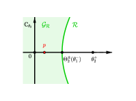
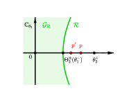
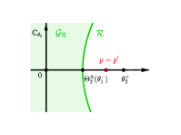
Figure 7: The curve \mathcal{R} in (20) is symmetric w.r.t. the horizontal axis, and 𝒢subscript𝒢\mathcal{G}_{\mathcal{R}} is the domain in green. The curve superscript\mathcal{R}^{-} is the half branch of \mathcal{R} with negative imaginary part. The points p𝑝p and q𝑞q are used to define the conformal mapping W𝑊W, see (18) and (27). The point q𝑞q is defined as follows: if the pole p𝑝p is in 𝒢subscript𝒢\mathcal{G}_{\mathcal{R}} then q=p𝑞𝑝q=p (figure on the left), otherwise q=12Θ2(θ1)𝑞12superscriptsubscriptΘ2superscriptsubscript𝜃1q=\frac{1}{2}\Theta_{2}^{-}(\theta_{1}^{-}) (figure on the right), see (25)

3 A proof of Theorem 1 via reduction to BVPs

3.1 Carleman BVP

For θ2subscript𝜃2\theta_{2}\in\mathcal{R}, define the function G𝐺G as in (13):

G(θ2)=γ1γ2(Θ1(θ2),θ2)γ2γ1(Θ1(θ2¯),θ2¯).𝐺subscript𝜃2subscript𝛾1subscript𝛾2superscriptsubscriptΘ1subscript𝜃2subscript𝜃2subscript𝛾2subscript𝛾1superscriptsubscriptΘ1¯subscript𝜃2¯subscript𝜃2G(\theta_{2})=\frac{\gamma_{1}}{\gamma_{2}}(\Theta_{1}^{-}(\theta_{2}),\theta_{2})\frac{\gamma_{2}}{\gamma_{1}}(\Theta_{1}^{-}(\overline{\theta_{2}}),\overline{\theta_{2}}).

Notice that G(θ2)G(θ2¯)=1𝐺subscript𝜃2𝐺¯subscript𝜃21G(\theta_{2})G(\overline{\theta_{2}})=1 and that for θ2subscript𝜃2\theta_{2}\in\mathcal{R} one has Θ1(θ2¯)=Θ1(θ2)superscriptsubscriptΘ1¯subscript𝜃2superscriptsubscriptΘ1subscript𝜃2\Theta_{1}^{-}(\overline{\theta_{2}})=\Theta_{1}^{-}({\theta_{2}}). Let us also recall that p𝑝p is defined in (18).

Proposition 6 (Carleman BVP with shift).

The function φ1subscript𝜑1\varphi_{1} in (4)

  1. (1)

    is meromorphic on 𝒢subscript𝒢\mathcal{G}_{\mathcal{R}},

    • without pole on 𝒢subscript𝒢\mathcal{G}_{\mathcal{R}} if γ1(θ1,Θ2(θ1))<0subscript𝛾1superscriptsubscript𝜃1superscriptsubscriptΘ2superscriptsubscript𝜃10\gamma_{1}(\theta_{1}^{-},\Theta_{2}^{-}(\theta_{1}^{-}))<0,

    • with a single pole on 𝒢subscript𝒢\mathcal{G}_{\mathcal{R}} at p𝑝p of order one if γ1(θ1,Θ2(θ1))>0subscript𝛾1superscriptsubscript𝜃1superscriptsubscriptΘ2superscriptsubscript𝜃10\gamma_{1}(\theta_{1}^{-},\Theta_{2}^{-}(\theta_{1}^{-}))>0,

    • without pole on 𝒢subscript𝒢\mathcal{G}_{\mathcal{R}} and with a single pole of order one on the boundary \mathcal{R} of 𝒢subscript𝒢\mathcal{G}_{\mathcal{R}}, at p=Θ2(θ1)𝑝superscriptsubscriptΘ2superscriptsubscript𝜃1p=\Theta_{2}^{-}(\theta_{1}^{-}), if γ1(θ1,Θ2(θ1))=0subscript𝛾1superscriptsubscript𝜃1superscriptsubscriptΘ2superscriptsubscript𝜃10\gamma_{1}(\theta_{1}^{-},\Theta_{2}^{-}(\theta_{1}^{-}))=0,

  2. (2)

    is continuous on 𝒢¯{p}¯subscript𝒢𝑝\overline{\mathcal{G}_{\mathcal{R}}}\setminus\{p\} and bounded at infinity,

  3. (3)

    satisfies the boundary condition

    φ1(θ2¯)=G(θ2)φ1(θ2),θ2.formulae-sequencesubscript𝜑1¯subscript𝜃2𝐺subscript𝜃2subscript𝜑1subscript𝜃2for-allsubscript𝜃2\varphi_{1}(\overline{\theta_{2}})=G(\theta_{2})\varphi_{1}({\theta_{2}}),\qquad\forall\theta_{2}\in\mathcal{R}. (22)

It is worth mentioning that the condition on the sign of γ1(θ1,Θ2(θ1))subscript𝛾1superscriptsubscript𝜃1superscriptsubscriptΘ2superscriptsubscript𝜃1\gamma_{1}(\theta_{1}^{-},\Theta_{2}^{-}(\theta_{1}^{-})) has a clear geometric meaning: indeed, γ1(θ1,Θ2(θ1))subscript𝛾1superscriptsubscript𝜃1superscriptsubscriptΘ2superscriptsubscript𝜃1\gamma_{1}(\theta_{1}^{-},\Theta_{2}^{-}(\theta_{1}^{-})) is negative (resp. positive) if and only if the straight line corresponding to γ1subscript𝛾1\gamma_{1} crosses the ellipse below (resp. above) the ordinate Θ2(θ1)superscriptsubscriptΘ2superscriptsubscript𝜃1\Theta_{2}^{-}(\theta_{1}^{-}); see Figure 3, left (resp. right).

Remark 7.

Item (1) of Proposition 6 shows that according to the values of the parameters, various cases exist regarding the singularities of the Laplace transform in the domain 𝒢subscript𝒢\mathcal{G}_{\mathcal{R}}. This is the reason why there isn’t a unique expression for the Laplace transform in our main Theorem 1, but two different expressions.

Proof of Proposition 6.

First of all, it follows from Lemma 3 that φ1subscript𝜑1\varphi_{1} is meromorphic in 𝒢subscript𝒢\mathcal{G}_{\mathcal{R}} and may have a pole of order one at p𝑝p. Indeed, due to the continuation formula (17), the only potential pole p𝑝p of φ1subscript𝜑1\varphi_{1} in 𝒢subscript𝒢\mathcal{G}_{\mathcal{R}} should be a zero of γ1subscript𝛾1\gamma_{1}. It is then on the real line and characterized by (18). Moreover, p𝑝p defined by (18) is smaller than Θ2(θ1)superscriptsubscriptΘ2superscriptsubscript𝜃1\Theta_{2}^{-}(\theta_{1}^{-}) (i.e., p𝒢𝑝subscript𝒢p\in\mathcal{G}_{\mathcal{R}}) if and only if the geometric condition γ1(θ1,Θ2(θ1))>0subscript𝛾1superscriptsubscript𝜃1superscriptsubscriptΘ2superscriptsubscript𝜃10\gamma_{1}(\theta_{1}^{-},\Theta_{2}^{-}(\theta_{1}^{-}))>0 is satisfied, see Figure 3. This demonstrates the first item of Proposition 6.

The second item (in particular the fact that φ1subscript𝜑1\varphi_{1} is bounded at infinity) comes from Lemma 3 together with the fact that (4) implies that φ1subscript𝜑1\varphi_{1} (resp. φ2subscript𝜑2\varphi_{2}) is bounded on the set {θ2:θ20}conditional-setsubscript𝜃2subscript𝜃20\{\theta_{2}\in\mathbb{C}:\Re\,\theta_{2}\leqslant 0\} (resp. {θ2:θ10}conditional-setsubscript𝜃2subscript𝜃10\{\theta_{2}\in\mathbb{C}:\Re\,\theta_{1}\leqslant 0\}).

To prove the boundary condition (22) (that we announced in [29, Proposition 7]), we consider θ1subscript𝜃1\theta_{1} such that θ1<0subscript𝜃10{\Re}\,\theta_{1}<0, and evaluate the functional equation (5) at (θ1,Θ2±(θ1))subscript𝜃1superscriptsubscriptΘ2plus-or-minussubscript𝜃1(\theta_{1},\Theta_{2}^{\pm}(\theta_{1})). This implies

γ1γ2(θ1,Θ2±(θ1))φ1(Θ2±(θ1))+φ2(θ1)=0,subscript𝛾1subscript𝛾2subscript𝜃1superscriptsubscriptΘ2plus-or-minussubscript𝜃1subscript𝜑1superscriptsubscriptΘ2plus-or-minussubscript𝜃1subscript𝜑2subscript𝜃10\frac{\gamma_{1}}{\gamma_{2}}(\theta_{1},\Theta_{2}^{\pm}(\theta_{1}))\varphi_{1}(\Theta_{2}^{\pm}(\theta_{1}))+\varphi_{2}(\theta_{1})=0,

which in turn yields

γ1γ2(θ1,Θ2+(θ1))φ1(Θ2+(θ1))=γ1γ2(θ1,Θ2(θ1))φ1(Θ2(θ1)).subscript𝛾1subscript𝛾2subscript𝜃1superscriptsubscriptΘ2subscript𝜃1subscript𝜑1superscriptsubscriptΘ2subscript𝜃1subscript𝛾1subscript𝛾2subscript𝜃1superscriptsubscriptΘ2subscript𝜃1subscript𝜑1superscriptsubscriptΘ2subscript𝜃1\frac{\gamma_{1}}{\gamma_{2}}(\theta_{1},\Theta_{2}^{+}(\theta_{1}))\varphi_{1}(\Theta_{2}^{+}(\theta_{1}))=\frac{\gamma_{1}}{\gamma_{2}}(\theta_{1},\Theta_{2}^{-}(\theta_{1}))\varphi_{1}(\Theta_{2}^{-}(\theta_{1})). (23)

Restricting (23) to values of θ1(,θ1)subscript𝜃1superscriptsubscript𝜃1\theta_{1}\in(-\infty,\theta_{1}^{-}), for which Θ2+(θ1)superscriptsubscriptΘ2subscript𝜃1\Theta_{2}^{+}(\theta_{1}) and Θ2(θ1)superscriptsubscriptΘ2subscript𝜃1\Theta_{2}^{-}(\theta_{1}) are complex conjugate (see Section 2), noting θ2=Θ2(θ1)subscript𝜃2superscriptsubscriptΘ2subscript𝜃1\theta_{2}=\Theta_{2}^{-}(\theta_{1})\in\mathcal{R} and noticing that θ1=Θ1(θ2)subscript𝜃1superscriptsubscriptΘ1subscript𝜃2\theta_{1}=\Theta_{1}^{-}(\theta_{2}), we reach the conclusion that

φ1(θ2¯)=γ1γ2(θ1,θ2)γ2γ1(θ1,θ2¯)φ1(θ2),subscript𝜑1¯subscript𝜃2subscript𝛾1subscript𝛾2subscript𝜃1subscript𝜃2subscript𝛾2subscript𝛾1subscript𝜃1¯subscript𝜃2subscript𝜑1subscript𝜃2\varphi_{1}(\overline{\theta_{2}})=\frac{\gamma_{1}}{\gamma_{2}}(\theta_{1},\theta_{2})\frac{\gamma_{2}}{\gamma_{1}}(\theta_{1},\overline{\theta_{2}})\varphi_{1}({\theta_{2}}),

which, by definition (13) of G𝐺G, exactly coincides with the boundary condition (22). Although we do not exclude a priori the denominators in (23) to vanish, note that this does not happen for θ1(,θ1)subscript𝜃1subscript𝜃1\theta_{1}\in(-\infty,\theta_{1}) since then the imaginary part of Θ2±(θ1)superscriptsubscriptΘ2plus-or-minussubscript𝜃1\Theta_{2}^{\pm}(\theta_{1}) is non-zero.

The BVP established in Proposition 6 belongs to the class of homogeneous Carleman (or Riemann-Carleman) BVPs with shift, see [44], the shift being here the complex conjugation.

In some cases, the function G𝐺G in (22) can be factorized, leading to an interesting particular case, that we comment below. As we shall see, the well-known skew-symmetric condition

2Σ=Rdiag(R)1diag(Σ)+diag(Σ)diag(R)1R2Σ𝑅diagsuperscript𝑅1diagΣdiagΣdiagsuperscript𝑅1superscript𝑅top2\Sigma=R\cdot\text{diag}(R)^{-1}\cdot\text{diag}(\Sigma)+\text{diag}(\Sigma)\cdot\text{diag}(R)^{-1}\cdot R^{\top} (24)

(equivalent for the stationary distribution π(x1,x2)𝜋subscript𝑥1subscript𝑥2\pi(x_{1},x_{2}) to have a product-form) gives a family of examples where such a factorization holds. In (24) we have noted diag(A)diag𝐴\text{diag}(A) the diagonal matrix with the same diagonal coefficients as those of A𝐴A.

Remark 8.

If there exists a rational function F𝐹F such that

G(θ2)=F(θ2)F(θ2¯),𝐺subscript𝜃2𝐹subscript𝜃2𝐹¯subscript𝜃2G(\theta_{2})=\frac{F(\theta_{2})}{F(\overline{\theta_{2}})},

one can transform the boundary condition (22) for φ1subscript𝜑1\varphi_{1} with G1𝐺1G\neq 1 into a boundary condition for φ1Fsubscript𝜑1𝐹\varphi_{1}\cdot F with G=1𝐺1G=1, namely,

(φ1F)(θ2¯)=(φ1F)(θ2).subscript𝜑1𝐹¯subscript𝜃2subscript𝜑1𝐹subscript𝜃2(\varphi_{1}\cdot F)(\overline{\theta_{2}})=(\varphi_{1}\cdot F)({\theta_{2}}).

Then the associated BVP should be solvable using Tutte’s invariants [3]. This is what has been done in [29], for the particular case of orthogonal reflections (corresponding to F(θ2)=1θ2𝐹subscript𝜃21subscript𝜃2F(\theta_{2})=\frac{1}{\theta_{2}}).

We show in Section 5.2 that such a rational function F𝐹F always exists in the skew-symmetric case (24), and from this we derive a rational expression of the Laplace transform.

The existence of a rational function F𝐹F factorizing G𝐺G as above is reminiscent of the notion of decoupling function or telescoper, introduced in [3, 21].

However, a rational factorization term F𝐹F as in Remark 8 does not exist in general, and it is still an open problem to characterize the parameters (Σ,μ,R)Σ𝜇𝑅(\Sigma,\mu,R) for which F𝐹F exists. As a consequence, we cannot systematically use Tutte’s invariants technique: we are left with transforming the BVP of Proposition 6 into a more classical one, using a certain conformal mapping having a very convenient gluing property.

3.2 Conformal gluing

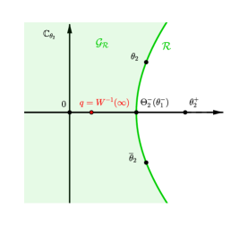
Our main result in this section is to prove that the function W𝑊W defined by Equation (27) below satisfies the properties of Lemma 9, allowing to transform the Carleman BVP with shift on the curve \mathcal{R} of Proposition 6 into a classical BVP on the segment [0,1]01[0,1].

Refer to caption
Refer to caption
Figure 8: Domains, curves and points related to the Carleman BVP with shift on \mathcal{R} (left) and the standard BVP on [0,1]01[0,1] (right)

First we need to define q𝑞q by

q={pif γ1(θ1,Θ2(θ1))>0, i.e., if φ1 admits p𝒢 as a pole,12Θ2(θ1)otherwise.𝑞cases𝑝if subscript𝛾1superscriptsubscript𝜃1superscriptsubscriptΘ2superscriptsubscript𝜃10 i.e., if φ1 admits p𝒢 as a pole12superscriptsubscriptΘ2superscriptsubscript𝜃1otherwiseq=\left\{\begin{array}[]{ll}p&\text{if }\gamma_{1}(\theta_{1}^{-},\Theta_{2}^{-}(\theta_{1}^{-}))>0,\text{ i.e., if $\varphi_{1}$ admits $p\in\mathcal{G}_{\mathcal{R}}$ as a pole},\vskip 3.0pt plus 1.0pt minus 1.0pt\\ \frac{1}{2}\Theta_{2}^{-}(\theta_{1}^{-})&\text{otherwise}.\end{array}\right. (25)

Note, the choice 12Θ2(θ1)12superscriptsubscriptΘ2superscriptsubscript𝜃1\frac{1}{2}\Theta_{2}^{-}(\theta_{1}^{-}) is arbitrary: any point in 𝒢subscript𝒢\mathcal{G}_{\mathcal{R}} would have been suitable. See Figures 3, 7 and 8. In the case where condition (15) is not satisfied, Θ2(θ1)superscriptsubscriptΘ2superscriptsubscript𝜃1\Theta_{2}^{-}(\theta_{1}^{-}) may be negative and another choice for q𝑞q should be done (as for example Θ2(θ1)1superscriptsubscriptΘ2superscriptsubscript𝜃11\Theta_{2}^{-}(\theta_{1}^{-})-1), see Section 3.6.

The function W𝑊W is built on the function w𝑤w below (note, w𝑤w is introduced in [29, Theorem 1]; under the symmetry conditions μ1=μ2subscript𝜇1subscript𝜇2\mu_{1}=\mu_{2}, σ11=σ22subscript𝜎11subscript𝜎22\sigma_{11}=\sigma_{22}, and symmetric reflection vectors in (1), Foschini [27] also obtained an expression for the conformal mapping w𝑤w, see [27, Figure 3]; see finally [2, Equation (4.6)] for a related formulation of w𝑤w):

w(θ2)=Tπβ(2θ2(θ2++θ2)θ2+θ2),𝑤subscript𝜃2subscript𝑇𝜋𝛽2subscript𝜃2superscriptsubscript𝜃2superscriptsubscript𝜃2superscriptsubscript𝜃2superscriptsubscript𝜃2w(\theta_{2})=T_{\frac{\pi}{\beta}}\left(-\frac{2\theta_{2}-(\theta_{2}^{+}+\theta_{2}^{-})}{\theta_{2}^{+}-\theta_{2}^{-}}\right),

which itself uses the branch points (8), the generalized Chebyshev polynomial (12) and the angle

β=arccosσ12σ11σ22.𝛽subscript𝜎12subscript𝜎11subscript𝜎22\beta=\arccos{-\frac{\sigma_{12}}{\sqrt{\sigma_{11}\sigma_{22}}}}. (26)

By [29, Section 4.2], w𝑤w is analytic on the cut plane [θ2+,)superscriptsubscript𝜃2\mathbb{C}\setminus[\theta_{2}^{+},\infty). Then we define

W(θ2)=w(θ2)w(Θ2(θ1))w(θ2)w(q)=w(θ2)+1w(θ2)w(q).𝑊subscript𝜃2𝑤subscript𝜃2𝑤superscriptsubscriptΘ2superscriptsubscript𝜃1𝑤subscript𝜃2𝑤𝑞𝑤subscript𝜃21𝑤subscript𝜃2𝑤𝑞W(\theta_{2})=\frac{w(\theta_{2})-w(\Theta_{2}^{-}(\theta_{1}^{-}))}{w(\theta_{2})-w(q)}=\frac{w(\theta_{2})+1}{w(\theta_{2})-w(q)}. (27)

The last equality is due to the identity

Θ2(θ1)=θ2++θ22θ2+θ22cosβ.superscriptsubscriptΘ2superscriptsubscript𝜃1superscriptsubscript𝜃2superscriptsubscript𝜃22superscriptsubscript𝜃2superscriptsubscript𝜃22𝛽\Theta_{2}^{-}(\theta_{1}^{-})=\frac{\theta_{2}^{+}+\theta_{2}^{-}}{2}-\frac{\theta_{2}^{+}-\theta_{2}^{-}}{2}\cos\beta.

We can see it by a direct computation or using a uniformization of the zero set of the kernel, see [29, Section 5] for more details. Then we have w(Θ2(θ1))=Tπβ(cosβ)=cosπ=1𝑤superscriptsubscriptΘ2superscriptsubscript𝜃1subscript𝑇𝜋𝛽𝛽𝜋1w(\Theta_{2}^{-}(\theta_{1}^{-}))=T_{\frac{\pi}{\beta}}(\cos\beta)=\cos\pi=-1.

Lemma 9.

The function W𝑊W in (27)

  1. (i)

    is analytic in 𝒢{q}subscript𝒢𝑞\mathcal{G}_{\mathcal{R}}\setminus\{q\}, continuous in 𝒢¯{q}¯subscript𝒢𝑞\overline{\mathcal{G}_{\mathcal{R}}}\setminus\{q\} and bounded at infinity,

  2. (ii)

    is one-to-one from 𝒢{q}subscript𝒢𝑞\mathcal{G}_{\mathcal{R}}\setminus\{q\} onto [0,1]01\mathbb{C}\setminus[0,1],

  3. (iii)

    satisfies W(θ2)=W(θ2¯)𝑊subscript𝜃2𝑊¯subscript𝜃2W(\theta_{2})=W(\overline{\theta_{2}}) for all θ2subscript𝜃2\theta_{2}\in\mathcal{R}.

Proof.

It can be found in [29, Lemma 6] that w𝑤w in (10)

  1. (i’)

    is analytic in 𝒢subscript𝒢\mathcal{G}_{\mathcal{R}}, continuous in 𝒢¯¯subscript𝒢\overline{\mathcal{G}_{\mathcal{R}}} and unbounded at infinity (Tasubscript𝑇𝑎T_{a} admits an analytic continuation on (θ2+,)superscriptsubscript𝜃2\mathbb{C}\setminus{\color[rgb]{0,0,0}(\theta_{2}^{+},\infty)}, and even on \mathbb{C} if a𝑎a is a non-negative integer: in that case Tasubscript𝑇𝑎T_{a} is the classical Chebyshev polynomial of the first kind),

  2. (ii’)

    is one-to-one from 𝒢subscript𝒢\mathcal{G}_{\mathcal{R}} onto (,1]1\mathbb{C}\setminus(-\infty,-1],

  3. (iii’)

    satisfies w(θ2)=w(θ2¯)𝑤subscript𝜃2𝑤¯subscript𝜃2w(\theta_{2})=w(\overline{\theta_{2}}) for all θ2subscript𝜃2\theta_{2}\in\mathcal{R}.

Here we want to define another conformal gluing function, which glues together the upper part and the lower part of the hyperbola onto the segment [0,1]01[0,1], and which sends the point q𝑞q in (25) at infinity, see Figure 8. For this reason we set W𝑊W as in (27): by construction W(Θ2(θ1))=0𝑊superscriptsubscriptΘ2superscriptsubscript𝜃10W(\Theta_{2}^{-}(\theta_{1}^{-}))=0, W()=1𝑊1W(\infty)=1 and W(q)=𝑊𝑞W(q)=\infty. The proof of Lemma 9 follows from the above-mentioned properties (i’)(iii’) of w𝑤w together with the definition (27) of W𝑊W. ∎

Remark 10.

The algebraic nature of the mapping w𝑤w in (10) (or equivalently W𝑊W in (27)) is directly related to the rationality of βπ𝛽𝜋\frac{\beta}{\pi}. Precisely, as shown in [29, Proposition 13], the following behaviors are possible:

  • The function w𝑤w is algebraic if and only if βπ𝛽𝜋\frac{\beta}{\pi}\in\mathbb{Q};

  • If in addition πβ𝜋𝛽\frac{\pi}{\beta}\in\mathbb{N} (and only in this case), then w𝑤w is a polynomial.

3.3 Reduction to a standard BVP

Thanks to the gluing function W𝑊W in (27), we are able to reformulate the Carleman BVP as a standard BVP for an open contour. See Figure 8 for a compact view of the two complex planes associated to the Carleman’s and Riemann’s BVPs. Define ψ1subscript𝜓1\psi_{1} by

ψ1(t)=φ1W1(t),t[0,1]formulae-sequencesubscript𝜓1𝑡subscript𝜑1superscript𝑊1𝑡for-all𝑡01\psi_{1}(t)=\varphi_{1}\circ W^{-1}(t),\qquad\forall t\in\mathbb{C}\setminus[0,1] (28)

(note, ψ1subscript𝜓1\psi_{1} is meromorphic on [0,1]01\mathbb{C}\setminus[0,1]). Equivalently we have φ1(θ2)=ψ1W(θ2)subscript𝜑1subscript𝜃2subscript𝜓1𝑊subscript𝜃2\varphi_{1}(\theta_{2})=\psi_{1}\circ W(\theta_{2}) for θ2𝒢subscript𝜃2subscript𝒢\theta_{2}\in\mathcal{G}_{\mathcal{R}}. Obviously W1superscript𝑊1W^{-1} is not well defined on [0,1]01[0,1]; however, it does admit upper and lower limits for t[0,1]𝑡01t\in[0,1]:

(W1)+(t)=limutu>0W1(u),(W1)(t)=limutu<0W1(u),formulae-sequencesuperscriptsuperscript𝑊1𝑡subscript𝑢𝑡𝑢0superscript𝑊1𝑢superscriptsuperscript𝑊1𝑡subscript𝑢𝑡𝑢0superscript𝑊1𝑢(W^{-1})^{+}(t)=\lim_{\begin{subarray}{c}u\to t\\ \Im u>0\end{subarray}}W^{-1}(u),\qquad(W^{-1})^{-}(t)=\lim_{\begin{subarray}{c}u\to t\\ \Im u<0\end{subarray}}W^{-1}(u),

and similarly for ψ1+(t)superscriptsubscript𝜓1𝑡\psi_{1}^{+}(t) and ψ1(t)superscriptsubscript𝜓1𝑡\psi_{1}^{-}(t). Then for θ2subscript𝜃2\theta_{2}\in\mathcal{R} and t=W(θ2)=W(θ2¯)𝑡𝑊subscript𝜃2𝑊¯subscript𝜃2t=W(\theta_{2})=W(\overline{\theta_{2}}), we have

φ1(θ2)={ψ1+(t)if θ2>0,ψ1(t)if θ2<0,φ1(θ2¯)={ψ1(t)if θ2>0,ψ1+(t)if θ2<0.formulae-sequencesubscript𝜑1subscript𝜃2casessuperscriptsubscript𝜓1𝑡if subscript𝜃20superscriptsubscript𝜓1𝑡if subscript𝜃20subscript𝜑1¯subscript𝜃2casessuperscriptsubscript𝜓1𝑡if subscript𝜃20superscriptsubscript𝜓1𝑡if subscript𝜃20\varphi_{1}({\theta_{2}})=\left\{\begin{array}[]{ll}\psi_{1}^{+}(t)&\text{if }\Im\,\theta_{2}>0,\vskip 3.0pt plus 1.0pt minus 1.0pt\\ \psi_{1}^{-}(t)&\text{if }\Im\,\theta_{2}<0,\end{array}\right.\qquad\varphi_{1}(\overline{\theta_{2}})=\left\{\begin{array}[]{ll}\psi_{1}^{-}(t)&\text{if }\Im\,\theta_{2}>0,\vskip 3.0pt plus 1.0pt minus 1.0pt\\ \psi_{1}^{+}(t)&\text{if }\Im\,\theta_{2}<0.\end{array}\right.

Define further

H(t)=G((W1)(t)),t[0,1].formulae-sequence𝐻𝑡𝐺superscriptsuperscript𝑊1𝑡for-all𝑡01H(t)=G((W^{-1})^{-}(t)),\qquad\forall t\in[0,1]. (29)

Then Proposition 6 becomes:

Proposition 11 (Riemann BVP).

The function ψ1subscript𝜓1\psi_{1} in (28)

  1. (1)

    is analytic in [0,1]01\mathbb{C}\setminus[0,1], bounded at infinity if γ1(θ1,Θ2(θ1))0subscript𝛾1superscriptsubscript𝜃1superscriptsubscriptΘ2superscriptsubscript𝜃10\gamma_{1}(\theta_{1}^{-},\Theta_{2}^{-}(\theta_{1}^{-}))\leqslant 0 and admitting a simple pole at infinity otherwise,

  2. (2)

    is continuous on [0,1]01[0,1] from below (with limits ψ1superscriptsubscript𝜓1\psi_{1}^{-}) and above (with limits ψ1+superscriptsubscript𝜓1\psi_{1}^{+}), bounded at 00 and 111 (except if γ1(θ1,Θ2(θ1))=0subscript𝛾1superscriptsubscript𝜃1superscriptsubscriptΘ2superscriptsubscript𝜃10\gamma_{1}(\theta_{1}^{-},\Theta_{2}^{-}(\theta_{1}^{-}))=0: in this case it has a pole of order one at 00),

  3. (3)

    satisfies, with H𝐻H defined in (29), the boundary condition

    ψ1+(t)=H(t)ψ1(t),t[0,1].formulae-sequencesuperscriptsubscript𝜓1𝑡𝐻𝑡superscriptsubscript𝜓1𝑡for-all𝑡01\psi_{1}^{+}(t)=H(t)\psi_{1}^{-}(t),\qquad\forall t\in[0,1]. (30)
Proof.

Items (1) and (2) directly follow from the corresponding items in Proposition 6. With the above definitions, the boundary equation (22) becomes

{ψ1(t)=G(θ2)ψ1+(t)if θ2>0,ψ1+(t)=G(θ2)ψ1(t)if θ2<0.casessuperscriptsubscript𝜓1𝑡𝐺subscript𝜃2superscriptsubscript𝜓1𝑡if subscript𝜃20superscriptsubscript𝜓1𝑡𝐺subscript𝜃2superscriptsubscript𝜓1𝑡if subscript𝜃20\left\{\begin{array}[]{ll}\psi_{1}^{-}(t)=G(\theta_{2})\psi_{1}^{+}(t)&\text{if }\Im\,\theta_{2}>0,\vskip 3.0pt plus 1.0pt minus 1.0pt\\ \psi_{1}^{+}(t)=G(\theta_{2})\psi_{1}^{-}(t)&\text{if }\Im\,\theta_{2}<0.\end{array}\right.

Since 1G(θ2)=G(θ2¯)=H(t)1𝐺subscript𝜃2𝐺¯subscript𝜃2𝐻𝑡\frac{1}{G(\theta_{2})}=G(\overline{\theta_{2}})=H(t) if θ2>0subscript𝜃20\Im\,\theta_{2}>0, and G(θ2)=H(t)𝐺subscript𝜃2𝐻𝑡G({\theta_{2}})=H(t) if θ2<0subscript𝜃20\Im\,\theta_{2}<0, the last item follows. ∎

3.4 Index of the BVP

The resolution of BVPs as in Proposition 11 heavily depends on the index χ𝜒\chi (see, e.g., [44, Section 5.2]), which is related to the variation of argument of H𝐻H on [0,1]01[0,1]:

Δ=[argH]01,d=argH(0)(π,π],χ=d+Δ2π.formulae-sequenceformulae-sequenceΔsuperscriptsubscriptdelimited-[]𝐻01𝑑𝐻0𝜋𝜋𝜒𝑑Δ2𝜋\Delta=[\arg H]_{0}^{1},\qquad{d}=\arg H(0)\in(-\pi,\pi],\qquad\chi=\left\lfloor\frac{{d}+\Delta}{2\pi}\right\rfloor. (31)

ΔΔ\Delta quantifies the variation of argument of H𝐻H on [0,1]01[0,1] and argH(1)=d+Δ𝐻1𝑑Δ\arg H(1)={d}+\Delta. Since (W1)([0,1])=superscriptsuperscript𝑊101superscript(W^{-1})^{-}([0,1])=\mathcal{R}^{-}, ΔΔ\Delta in (31) can be equivalently written [argG]subscriptdelimited-[]𝐺superscript[\arg G]_{\mathcal{R}^{-}} (from the vertex to infinity).

Remark 12.

It is important to notice that d(π,π]𝑑𝜋𝜋{d}\in(-\pi,\pi] in (31) corresponds to an arbitrary choice. Any other choice would eventually lead to the same Theorem 1 (though written slightly differently).

First, we compute d𝑑{d} in (31).

Lemma 13.

We have

d={0if γ1(θ1,Θ2(θ1))0,πif γ1(θ1,Θ2(θ1))=0.𝑑cases0if subscript𝛾1superscriptsubscript𝜃1superscriptsubscriptΘ2superscriptsubscript𝜃10𝜋if subscript𝛾1superscriptsubscript𝜃1superscriptsubscriptΘ2superscriptsubscript𝜃10{d}=\left\{\begin{array}[]{ll}0&\text{if }\gamma_{1}(\theta_{1}^{-},\Theta_{2}^{-}(\theta_{1}^{-}))\neq 0,\vskip 3.0pt plus 1.0pt minus 1.0pt\\ \pi&\text{if }\gamma_{1}(\theta_{1}^{-},\Theta_{2}^{-}(\theta_{1}^{-}))=0.\end{array}\right. (32)

The angle d+Δ(2π,2π)𝑑Δ2𝜋2𝜋{d}+\Delta\in(-2\pi,2\pi) and we have

tand+Δ2=detRdetΣσ12(r11r22+r12r21)σ22r11r12σ11r22r21.𝑑Δ2𝑅Σsubscript𝜎12subscript𝑟11subscript𝑟22subscript𝑟12subscript𝑟21subscript𝜎22subscript𝑟11subscript𝑟12subscript𝜎11subscript𝑟22subscript𝑟21\tan\frac{{d}+\Delta}{2}=\frac{\det R\cdot{\color[rgb]{0,0,0}\sqrt{\det\Sigma}}}{\sigma_{12}(r_{11}r_{22}+r_{12}r_{21})-\sigma_{22}r_{11}r_{12}-\sigma_{11}r_{22}r_{21}}. (33)

Note that the denominator of (33) can be negative, zero or positive, depending on the parameters.

Proof of Lemma 13.

First of all we show the formula (32). If first γ1(θ1,Θ2(θ1))0subscript𝛾1superscriptsubscript𝜃1superscriptsubscriptΘ2superscriptsubscript𝜃10\gamma_{1}(\theta_{1}^{-},\Theta_{2}^{-}(\theta_{1}^{-}))\neq 0 then H(0)=G(Θ2(θ1))=1𝐻0𝐺superscriptsubscriptΘ2superscriptsubscript𝜃11H(0)=G(\Theta_{2}^{-}(\theta_{1}^{-}))=1, since Θ2(θ1)superscriptsubscriptΘ2superscriptsubscript𝜃1\Theta_{2}^{-}(\theta_{1}^{-})\in\mathbb{R} simplifies the quotient (13) and then d=argH(0)=0𝑑𝐻00{d}=\arg H(0)=0. In the other case γ1(θ1,Θ2(θ1))=0subscript𝛾1superscriptsubscript𝜃1superscriptsubscriptΘ2superscriptsubscript𝜃10\gamma_{1}(\theta_{1}^{-},\Theta_{2}^{-}(\theta_{1}^{-}))=0, and we have

limt0H(t)=limθ2Θ2(θ1)θ2θ2Θ2(θ1)θ2¯Θ2(θ1)=1.subscript𝑡0𝐻𝑡subscriptFRACOPsubscript𝜃2superscriptsubscriptΘ2superscriptsubscript𝜃1subscript𝜃2superscriptsubscript𝜃2superscriptsubscriptΘ2superscriptsubscript𝜃1¯subscript𝜃2superscriptsubscriptΘ2superscriptsubscript𝜃11\lim_{t\to 0}H(t)=\lim_{\theta_{2}\to\Theta_{2}^{-}(\theta_{1}^{-})\atop\theta_{2}\in\mathcal{R}^{-}}\frac{\theta_{2}-\Theta_{2}^{-}(\theta_{1}^{-})}{\overline{\theta_{2}}-\Theta_{2}^{-}(\theta_{1}^{-})}=-1.

The last equality is due to the fact that the tangent to \mathcal{R} at Θ2(θ1)superscriptsubscriptΘ2superscriptsubscript𝜃1\Theta_{2}^{-}(\theta_{1}^{-}) is vertical, see Figure 8. Indeed if we write θ2Θ2(θ1)=a+ibsubscript𝜃2superscriptsubscriptΘ2superscriptsubscript𝜃1𝑎𝑖𝑏\theta_{2}-\Theta_{2}^{-}(\theta_{1}^{-})=a+ib when θ2Θ2(θ1)subscript𝜃2superscriptsubscriptΘ2superscriptsubscript𝜃1\theta_{2}\to\Theta_{2}^{-}(\theta_{1}^{-}) with θ2subscript𝜃2superscript\theta_{2}\in\mathcal{R}^{-}, the vertical tangent gives ab0𝑎𝑏0\frac{a}{b}\to 0 and then limt0H(t)=limab0ab+iabi=1subscript𝑡0𝐻𝑡subscript𝑎𝑏0𝑎𝑏𝑖𝑎𝑏𝑖1\lim_{t\to 0}H(t)=\lim_{\frac{a}{b}\to 0}\frac{\frac{a}{b}+i}{\frac{a}{b}-i}=-1. It implies that d=π𝑑𝜋{d}=\pi.

We are now going to show (33). We start by remarking that for θ2subscript𝜃2\theta_{2}\in\mathcal{R}, G(θ2)=1𝐺subscript𝜃21G(\theta_{2})=1 if and only if θ2subscript𝜃2\theta_{2}\in\mathbb{R}. Accordingly, for t[0,1]𝑡01t\in[0,1], H(t)=1𝐻𝑡1H(t)=1 only at t=0𝑡0t=0. Since |H|=1𝐻1|H|=1 on [0,1]01[0,1], then necessarily d+Δ[2π,2π]𝑑Δ2𝜋2𝜋{d}+\Delta\in[-2\pi,2\pi]. We now calculate

H(1)=limθ2θ2G(θ2).𝐻1subscriptFRACOPsubscript𝜃2subscript𝜃2superscript𝐺subscript𝜃2H(1)=\lim_{\theta_{2}\to\infty\hskip 2.84526pt\atop\theta_{2}\in\mathcal{R}^{-}}G(\theta_{2}).

Thanks to Equation (7) we easily compute the following limit

limθ2θ2Θ1(θ2)θ2=σ12idetΣσ11.subscriptFRACOPsubscript𝜃2subscript𝜃2superscriptsuperscriptsubscriptΘ1subscript𝜃2subscript𝜃2subscript𝜎12𝑖Σsubscript𝜎11\lim_{\theta_{2}\to\infty\hskip 2.84526pt\atop\theta_{2}\in\mathcal{R}^{-}}\frac{\Theta_{1}^{-}(\theta_{2})}{\theta_{2}}=\frac{-\sigma_{12}-i\sqrt{\det\Sigma}}{\sigma_{11}}.

Using this limit together with the definition of G𝐺G (see (13))

G(θ2)=(r11Θ1(θ2)θ2+r21)(r12Θ1(θ2)θ2¯+r22)(r12Θ1(θ2)θ2+r22)(r11Θ1(θ2)θ2¯+r21),𝐺subscript𝜃2subscript𝑟11superscriptsubscriptΘ1subscript𝜃2subscript𝜃2subscript𝑟21subscript𝑟12superscriptsubscriptΘ1subscript𝜃2¯subscript𝜃2subscript𝑟22subscript𝑟12superscriptsubscriptΘ1subscript𝜃2subscript𝜃2subscript𝑟22subscript𝑟11superscriptsubscriptΘ1subscript𝜃2¯subscript𝜃2subscript𝑟21G(\theta_{2})=\frac{\big{(}r_{11}\frac{\Theta_{1}^{-}(\theta_{2})}{\theta_{2}}+r_{21}\big{)}\big{(}r_{12}\frac{\Theta_{1}^{-}(\theta_{2})}{\overline{\theta_{2}}}+r_{22}\big{)}}{\big{(}r_{12}\frac{\Theta_{1}^{-}(\theta_{2})}{\theta_{2}}+r_{22}\big{)}\big{(}r_{11}\frac{\Theta_{1}^{-}(\theta_{2})}{\overline{\theta_{2}}}+r_{21}\big{)}},

we obtain that

H(1)𝐻1\displaystyle H(1) =(r11(σ12idetΣ)+r21σ11)(r12(σ12+idetΣ)+r22σ11)(r12(σ12idetΣ)+r22σ11)(r11(σ12+idetΣ)+r21σ11)absentsubscript𝑟11subscript𝜎12𝑖Σsubscript𝑟21subscript𝜎11subscript𝑟12subscript𝜎12𝑖Σsubscript𝑟22subscript𝜎11subscript𝑟12subscript𝜎12𝑖Σsubscript𝑟22subscript𝜎11subscript𝑟11subscript𝜎12𝑖Σsubscript𝑟21subscript𝜎11\displaystyle=\frac{\big{(}r_{11}(-\sigma_{12}-i\sqrt{\det\Sigma})+r_{21}\sigma_{11}\big{)}\big{(}r_{12}(-\sigma_{12}+i\sqrt{\det\Sigma})+r_{22}\sigma_{11}\big{)}}{\big{(}r_{12}(-\sigma_{12}-i\sqrt{\det\Sigma})+r_{22}\sigma_{11}\big{)}\big{(}r_{11}(-\sigma_{12}+i\sqrt{\det\Sigma})+r_{21}\sigma_{11}\big{)}}
=σ22r11r12+σ11r22r21σ12(r11r22+r12r21)idetRdetΣσ22r11r12+σ11r22r21σ12(r11r22+r12r21)+idetRdetΣ=exp(i(d+Δ)).absentsubscript𝜎22subscript𝑟11subscript𝑟12subscript𝜎11subscript𝑟22subscript𝑟21subscript𝜎12subscript𝑟11subscript𝑟22subscript𝑟12subscript𝑟21𝑖𝑅Σsubscript𝜎22subscript𝑟11subscript𝑟12subscript𝜎11subscript𝑟22subscript𝑟21subscript𝜎12subscript𝑟11subscript𝑟22subscript𝑟12subscript𝑟21𝑖𝑅Σ𝑖𝑑Δ\displaystyle=\frac{\sigma_{22}r_{11}r_{12}+\sigma_{11}r_{22}r_{21}-\sigma_{12}(r_{11}r_{22}+r_{12}r_{21})-i\det R{\color[rgb]{0,0,0}\sqrt{\det\Sigma}}}{\sigma_{22}r_{11}r_{12}+\sigma_{11}r_{22}r_{21}-\sigma_{12}(r_{11}r_{22}+r_{12}r_{21})+i\det R{\color[rgb]{0,0,0}\sqrt{\det\Sigma}}}=\exp({i({d}+\Delta)}).

Remembering that argH(1)=d+Δ[2π,2π]𝐻1𝑑Δ2𝜋2𝜋\arg H(1)={d}+\Delta\in[-2\pi,2\pi], it gives (33) and clearly, d+Δ𝑑Δ{d}+\Delta cannot be equal to ±2πplus-or-minus2𝜋\pm 2\pi because detRdetΣ0𝑅Σ0\det R\cdot\det\Sigma\neq 0. ∎

We now prove that

χ={0if γ1(θ1,Θ2(θ1))0,1if γ1(θ1,Θ2(θ1))>0.𝜒cases0if subscript𝛾1superscriptsubscript𝜃1superscriptsubscriptΘ2superscriptsubscript𝜃101if subscript𝛾1superscriptsubscript𝜃1superscriptsubscriptΘ2superscriptsubscript𝜃10\chi=\left\{\begin{array}[]{rl}0&\displaystyle\text{if }\gamma_{1}(\theta_{1}^{-},\Theta_{2}^{-}(\theta_{1}^{-}))\leqslant 0,\vskip 3.0pt plus 1.0pt minus 1.0pt\\ -1&\displaystyle\text{if }\gamma_{1}(\theta_{1}^{-},\Theta_{2}^{-}(\theta_{1}^{-}))>0.\end{array}\right. (34)

In particular, χ𝜒\chi is an intrinsically non-continuous function of the parameters, see also Remark 7.

Recall that the function ψ1subscript𝜓1\psi_{1} has been defined in (28).

Lemma 14.

The index χ𝜒\chi can take only the values 00 and 11-1, and we have the dichotomy:

  • χ=0γ1(θ1,Θ2(θ1))0𝜒0subscript𝛾1superscriptsubscript𝜃1superscriptsubscriptΘ2superscriptsubscript𝜃10absent\chi=0\phantom{-}\Longleftrightarrow\gamma_{1}(\theta_{1}^{-},\Theta_{2}^{-}(\theta_{1}^{-}))\leqslant 0\Longleftrightarrow ψ1subscript𝜓1\psi_{1} has no pole at infinity,

  • χ=1γ1(θ1,Θ2(θ1))>0𝜒1subscript𝛾1superscriptsubscript𝜃1superscriptsubscriptΘ2superscriptsubscript𝜃10absent\chi=-1\Longleftrightarrow\gamma_{1}(\theta_{1}^{-},\Theta_{2}^{-}(\theta_{1}^{-}))>0\Longleftrightarrow ψ1subscript𝜓1\psi_{1} has a simple pole at infinity.

Note that a simple pole at infinity means that ψ1(t)ctsubscript𝜓1𝑡subscriptsimilar-to𝑐𝑡\displaystyle\psi_{1}(t)\mathop{\sim}_{\infty}c\cdot t for some non-zero constant c𝑐c.

Proof.

We have already seen in Proposition 6 that the sign of γ1(θ1,Θ2(θ1))subscript𝛾1superscriptsubscript𝜃1superscriptsubscriptΘ2superscriptsubscript𝜃1\gamma_{1}(\theta_{1}^{-},\Theta_{2}^{-}(\theta_{1}^{-})) determines whether φ1subscript𝜑1\varphi_{1} has a pole in 𝒢subscript𝒢\mathcal{G}_{\mathcal{R}} or not, and thus if ψ1subscript𝜓1\psi_{1} has a pole at infinity by the correspondence of Figure 8. This shows the two equivalences on the right in the statement of Lemma 14. We are thus left with proving the first two equivalent conditions.

First, if γ1(θ1,Θ2(θ1))=0subscript𝛾1superscriptsubscript𝜃1superscriptsubscriptΘ2superscriptsubscript𝜃10\gamma_{1}(\theta_{1}^{-},\Theta_{2}^{-}(\theta_{1}^{-}))=0, d=π𝑑𝜋{d}=\pi and we have seen that in this case H(t)1𝐻𝑡1H(t)\neq 1 for all t[0,1]𝑡01t\in[0,1]. By (31), we deduce that χ=0𝜒0\chi=0.

If now γ1(θ1,Θ2(θ1))0subscript𝛾1superscriptsubscript𝜃1superscriptsubscriptΘ2superscriptsubscript𝜃10\gamma_{1}(\theta_{1}^{-},\Theta_{2}^{-}(\theta_{1}^{-}))\neq 0 we notice that

χ=Δ2π=0 or 1.𝜒Δ2𝜋0 or 1\chi=\left\lfloor\frac{\Delta}{2\pi}\right\rfloor=0\text{ or }-1.

Indeed, we have proved in Lemma 13 that Δ(2π,2π)Δ2𝜋2𝜋\Delta\in(-2\pi,2\pi). In particular, the sign of ΔΔ\Delta determines χ𝜒\chi: if sgnΔ0sgnΔ0\operatorname{sgn}\Delta\geqslant 0 then χ=0𝜒0\chi=0 and if sgnΔ<0sgnΔ0\operatorname{sgn}\Delta<0, χ=1𝜒1\chi=-1. In the rest of the proof, we show that sgnΔ=sgnγ1(θ1,Θ2(θ1))sgnΔsgnsubscript𝛾1superscriptsubscript𝜃1superscriptsubscriptΘ2superscriptsubscript𝜃1\operatorname{sgn}\Delta=-\operatorname{sgn}\gamma_{1}(\theta_{1}^{-},\Theta_{2}^{-}(\theta_{1}^{-})). First, ΔΔ\Delta can be computed as

Δ=argH(1)=[argG]=[argγ1γ2¯γ2γ1¯(Θ1(θ2),θ2)].Δ𝐻1subscriptdelimited-[]𝐺superscriptsubscriptdelimited-[]subscript𝛾1¯subscript𝛾2subscript𝛾2¯subscript𝛾1superscriptsubscriptΘ1subscript𝜃2subscript𝜃2superscript\Delta=\arg H(1)=[\arg G]_{\mathcal{R}^{-}}=\left[\arg\frac{\gamma_{1}\overline{\gamma_{2}}}{\gamma_{2}\overline{\gamma_{1}}}(\Theta_{1}^{-}(\theta_{2}),\theta_{2})\right]_{\mathcal{R}^{-}}.

Let θ2=aibsubscript𝜃2𝑎𝑖𝑏superscript\theta_{2}=a-ib\in\mathcal{R}^{-} (we must have b0𝑏0b\geqslant 0 and aΘ2(θ1)>0𝑎superscriptsubscriptΘ2superscriptsubscript𝜃10a\geqslant\Theta_{2}^{-}(\theta_{1}^{-})>0, see Figure 7) and θ1=Θ1(θ2)(,θ1]subscript𝜃1superscriptsubscriptΘ1subscript𝜃2superscriptsubscript𝜃1\theta_{1}=\Theta_{1}^{-}(\theta_{2})\in(-\infty,\theta_{1}^{-}]. Using the expression (6) of γ1subscript𝛾1\gamma_{1} and γ2subscript𝛾2\gamma_{2}, we obtain

γ1γ2¯(θ1,θ2)=γ1(θ1,a)γ2(θ1,a)+r21r22b2+ibθ1detR,subscript𝛾1¯subscript𝛾2subscript𝜃1subscript𝜃2subscript𝛾1subscript𝜃1𝑎subscript𝛾2subscript𝜃1𝑎subscript𝑟21subscript𝑟22superscript𝑏2𝑖𝑏subscript𝜃1𝑅\gamma_{1}\overline{\gamma_{2}}(\theta_{1},\theta_{2})=\gamma_{1}(\theta_{1},a)\gamma_{2}(\theta_{1},a)+r_{21}r_{22}b^{2}+ib\theta_{1}\det R,

from where we deduce that

argγ1γ2¯γ2γ1¯(θ1,θ2)=2arctanbθ1detRγ1(θ1,a)γ2(θ1,a)+r21r22b2.subscript𝛾1¯subscript𝛾2subscript𝛾2¯subscript𝛾1subscript𝜃1subscript𝜃22𝑏subscript𝜃1𝑅subscript𝛾1subscript𝜃1𝑎subscript𝛾2subscript𝜃1𝑎subscript𝑟21subscript𝑟22superscript𝑏2\arg\frac{\gamma_{1}\overline{\gamma_{2}}}{\gamma_{2}\overline{\gamma_{1}}}(\theta_{1},\theta_{2})=2\arctan\frac{b\cdot\theta_{1}\cdot\det R}{\gamma_{1}(\theta_{1},a)\gamma_{2}(\theta_{1},a)+r_{21}r_{22}b^{2}}. (35)

We now look for the sign of (35) when θ2Θ2(θ1)subscript𝜃2superscriptsubscriptΘ2superscriptsubscript𝜃1\theta_{2}\to\Theta_{2}^{-}(\theta_{1}^{-}), while remaining in superscript\mathcal{R}^{-}. This is sufficient to give the sign of ΔΔ\Delta, because (35) does not change sign on superscript\mathcal{R}^{-} due to the fact that G(θ2)=1𝐺subscript𝜃21G(\theta_{2})=1 on superscript\mathcal{R}^{-} if and only if θ2=Θ2(θ1)subscript𝜃2superscriptsubscriptΘ2superscriptsubscript𝜃1\theta_{2}=\Theta_{2}^{-}(\theta_{1}^{-}).

When θ2Θ2(θ1)subscript𝜃2superscriptsubscriptΘ2superscriptsubscript𝜃1\theta_{2}\to\Theta_{2}^{-}(\theta_{1}^{-}) we have b0𝑏0b\to 0, aΘ2(θ1)𝑎superscriptsubscriptΘ2superscriptsubscript𝜃1a\to\Theta_{2}^{-}(\theta_{1}^{-}) and θ1θ1subscript𝜃1superscriptsubscript𝜃1\theta_{1}\to\theta_{1}^{-}. We thus have

sgnargγ1γ2¯γ2γ1¯(θ1,θ2)sgnsubscript𝛾1¯subscript𝛾2subscript𝛾2¯subscript𝛾1subscript𝜃1subscript𝜃2\displaystyle\operatorname{sgn}\arg\frac{\gamma_{1}\overline{\gamma_{2}}}{\gamma_{2}\overline{\gamma_{1}}}(\theta_{1},\theta_{2}) =sgnbsgnθ1sgndetRsgnγ2(θ1,Θ2(θ1))sgnγ1(θ1,Θ2(θ1))absentsgn𝑏sgnsubscript𝜃1sgn𝑅sgnsubscript𝛾2superscriptsubscript𝜃1superscriptsubscriptΘ2superscriptsubscript𝜃1sgnsubscript𝛾1superscriptsubscript𝜃1superscriptsubscriptΘ2superscriptsubscript𝜃1\displaystyle=\operatorname{sgn}b\cdot\operatorname{sgn}\theta_{1}\cdot\operatorname{sgn}\det R\cdot\operatorname{sgn}\gamma_{2}(\theta_{1}^{-},\Theta_{2}^{-}(\theta_{1}^{-}))\cdot\operatorname{sgn}\gamma_{1}(\theta_{1}^{-},\Theta_{2}^{-}(\theta_{1}^{-}))
=(+1)(1)(+1)(+1)sgnγ1(θ1,Θ2(θ1))absent1111sgnsubscript𝛾1superscriptsubscript𝜃1superscriptsubscriptΘ2superscriptsubscript𝜃1\displaystyle=(+1)(-1)(+1)(+1)\operatorname{sgn}\gamma_{1}(\theta_{1}^{-},\Theta_{2}^{-}(\theta_{1}^{-}))
=sgnγ1(θ1,Θ2(θ1)),absentsgnsubscript𝛾1superscriptsubscript𝜃1superscriptsubscriptΘ2superscriptsubscript𝜃1\displaystyle=-\operatorname{sgn}\gamma_{1}(\theta_{1}^{-},\Theta_{2}^{-}(\theta_{1}^{-})),

because b0𝑏0b\geqslant 0, θ1<0subscript𝜃10\theta_{1}<0, detR>0𝑅0\det R>0 by (2), and γ2(θ1,Θ2(θ1))>0subscript𝛾2superscriptsubscript𝜃1superscriptsubscriptΘ2superscriptsubscript𝜃10\gamma_{2}(\theta_{1}^{-},\Theta_{2}^{-}(\theta_{1}^{-}))>0 (because r22>0subscript𝑟220r_{22}>0 and r22μ1r12μ2<0subscript𝑟22subscript𝜇1subscript𝑟12subscript𝜇20r_{22}\mu_{1}-r_{12}\mu_{2}<0, see Figure 3 to visualize this geometric condition). Then sgnΔ=sgnargγ1γ2¯γ2γ1¯(θ1,θ2)=sgnγ1(θ1,Θ2(θ1))sgnΔsgnsubscript𝛾1¯subscript𝛾2subscript𝛾2¯subscript𝛾1subscript𝜃1subscript𝜃2sgnsubscript𝛾1superscriptsubscript𝜃1superscriptsubscriptΘ2superscriptsubscript𝜃1\operatorname{sgn}\Delta=\operatorname{sgn}\arg\frac{\gamma_{1}\overline{\gamma_{2}}}{\gamma_{2}\overline{\gamma_{1}}}(\theta_{1},\theta_{2})=-\operatorname{sgn}\gamma_{1}(\theta_{1}^{-},\Theta_{2}^{-}(\theta_{1}^{-})), concluding the proof. ∎

3.5 Resolution of the BVP

We are now in position to conclude the proof of Theorem 1. Reformulating Proposition 11, the function ψ1subscript𝜓1\psi_{1} in (28)

  • is sectionally analytic in [0,1]01\mathbb{C}\setminus[0,1],

  • is continuous on [0,1]01[0,1] from below (with limits ψ1superscriptsubscript𝜓1\psi_{1}^{-}) and above (with limits ψ1+superscriptsubscript𝜓1\psi_{1}^{+}),

    • \bullet

      is bounded at the vicinities of [0,1]01[0,1] if γ1(θ1,Θ2(θ1))0subscript𝛾1superscriptsubscript𝜃1superscriptsubscriptΘ2superscriptsubscript𝜃10\gamma_{1}(\theta_{1}^{-},\Theta_{2}^{-}(\theta_{1}^{-}))\neq 0,

    • \bullet

      has a pole of order one at 00 and bounded at 111 if γ1(θ1,Θ2(θ1))=0subscript𝛾1superscriptsubscript𝜃1superscriptsubscriptΘ2superscriptsubscript𝜃10\gamma_{1}(\theta_{1}^{-},\Theta_{2}^{-}(\theta_{1}^{-}))=0,

  • is bounded at infinity if there is no pole before Θ2(θ1)superscriptsubscriptΘ2superscriptsubscript𝜃1\Theta_{2}^{-}(\theta_{1}^{-}) (then taking the value φ1(q)subscript𝜑1𝑞\varphi_{1}(q)), and with a pole of order one (see Lemma 3) at infinity if not (in short, it has a pole of order χ𝜒-\chi at infinity),

  • satisfies ψ1+(t)=H(t)ψ1(t)superscriptsubscript𝜓1𝑡𝐻𝑡superscriptsubscript𝜓1𝑡\psi_{1}^{+}(t)=H(t)\psi_{1}^{-}(t) for t[0,1]𝑡01t\in[0,1], with index χ𝜒\chi given by (34), cf. also Lemma 14.

End of proof of Theorem 1.

Our main reference for the resolution of the above so-called homogeneous BVP on an open contour is the book [46] of Muskhelishvili, see in particular [46, §79].

First of all, we prove that there exists a non-zero constant c𝑐c such that

ψ1(t)=c(t1)χexpΓ(t),subscript𝜓1𝑡𝑐superscript𝑡1𝜒Γ𝑡\psi_{1}(t)=c(t-1)^{-\chi}\exp\Gamma(t), (36)

where ΓΓ\Gamma is the following function, sectionally analytic on [0,1]01\mathbb{C}\setminus[0,1]:

Γ(t)=12iπ01logH(z)ztdz.Γ𝑡12𝑖𝜋superscriptsubscript01𝐻𝑧𝑧𝑡differential-d𝑧\Gamma(t)=\frac{1}{2i\pi}\int_{0}^{1}\frac{\log H(z)}{z-t}\mathrm{d}z. (37)

To make precise the definition (37), we define logH(z)𝐻𝑧\log H(z) by the facts that it should vary continuously over [0,1]01[0,1], and its initial value is such that logH(0)=id𝐻0𝑖𝑑\log H(0)=i{d} (i.e., 00 if H(0)=1𝐻01H(0)=1 and iπ𝑖𝜋i\pi if H(0)=1𝐻01H(0)=-1, see (32)).

At the vicinities 00 and 111, we have by [46, §29 and §79] that

expΓ(t)=td2πΩ0(t),expΓ(t)=(t1)d+Δ2πΩ1(t),formulae-sequenceΓ𝑡superscript𝑡𝑑2𝜋subscriptΩ0𝑡Γ𝑡superscript𝑡1𝑑Δ2𝜋subscriptΩ1𝑡\exp{\Gamma(t)}=t^{-\frac{{d}}{2\pi}}\Omega_{0}(t),\qquad\exp{\Gamma(t)}=(t-1)^{\frac{{d}+\Delta}{2\pi}}\Omega_{1}(t), (38)

for some function Ω0subscriptΩ0\Omega_{0} (resp. Ω1subscriptΩ1\Omega_{1}) analytic in a neighborhood of 00 (resp. 111) and non-zero at 00 (resp. 111). Then we set

X(t)=tdπ(t1)χexpΓ(t).𝑋𝑡superscript𝑡𝑑𝜋superscript𝑡1𝜒Γ𝑡X(t)=t^{\frac{{d}}{\pi}}(t-1)^{-\chi}\exp{\Gamma(t)}. (39)

The function X𝑋X in (39) is sectionally analytic in [0,1]01\mathbb{C}\setminus[0,1], and by construction of ΓΓ\Gamma and the Sokhotski-Plemelj formulas, it satisfies the boundary condition (30) (see [46, §79] for more details). Furthermore it has a pole of order χ+dπ𝜒𝑑𝜋-\chi+\frac{{d}}{\pi} at infinity and is bounded at 00 and 111: indeed, dπ𝑑𝜋\frac{{d}}{\pi} and χ𝜒-\chi are both equal to 00 or 111, see Lemmas 13 and 14. Then we consider two cases separately.

\bullet First case: γ1(θ1,Θ2(θ1))0subscript𝛾1superscriptsubscript𝜃1superscriptsubscriptΘ2superscriptsubscript𝜃10\gamma_{1}(\theta_{1}^{-},\Theta_{2}^{-}(\theta_{1}^{-}))\neq 0. Then d=0𝑑0{d}=0, and the function X𝑋X in (39) simplifies into

X(t)=(t1)χexpΓ(t).𝑋𝑡superscript𝑡1𝜒Γ𝑡X(t)=(t-1)^{-\chi}\exp{\Gamma(t)}.

It satisfies the exact same boundary condition as (30). Looking at the ratio ψ1Xsubscript𝜓1𝑋\frac{\psi_{1}}{X}, the boundary condition (30) gives that on [0,1]01[0,1],

ψ1+X+=ψ1X.superscriptsubscript𝜓1superscript𝑋superscriptsubscript𝜓1superscript𝑋\frac{\psi_{1}^{+}}{X^{+}}=\frac{\psi_{1}^{-}}{X^{-}}.

The above ratio is then analytic in the entire plane, even at the vicinities 00 and 111. The point 00 is a regular point and 111 is a removable singularity. Indeed, 111 is an isolated singular point, at which ψ1Xsubscript𝜓1𝑋\frac{\psi_{1}}{X} might be infinite with degree less than unity (namely, χ+Δ2π𝜒Δ2𝜋-\chi+\frac{\Delta}{2\pi}). Moreover, the function ψ1Xsubscript𝜓1𝑋\frac{\psi_{1}}{X} is bounded at infinity, because both X𝑋X and ψ1subscript𝜓1\psi_{1} have a pole of the same order χ𝜒-\chi. Thanks to Liouville’s theorem, we deduce that ψ1Xsubscript𝜓1𝑋\frac{\psi_{1}}{X} is constant. In conclusion, the formula (36) holds in this case.

\bullet Second case: γ1(θ1,Θ2(θ1))=0subscript𝛾1superscriptsubscript𝜃1superscriptsubscriptΘ2superscriptsubscript𝜃10\gamma_{1}(\theta_{1}^{-},\Theta_{2}^{-}(\theta_{1}^{-}))=0. Then d=π𝑑𝜋{d}=\pi, χ=0𝜒0\chi=0 and X(t)=texpΓ(t)𝑋𝑡𝑡Γ𝑡X(t)=t\exp{\Gamma(t)} in (39). Firstly, we notice that the function tψ1𝑡subscript𝜓1t\psi_{1} satisfies the boundary condition (30), is bounded at 00 and 111, and has a pole of order one at infinity. Moreover, the function X𝑋X has a pole of order 111 at infinity. Considering then the ratio tψ1X𝑡subscript𝜓1𝑋\frac{t\psi_{1}}{X}, the boundary condition (30) implies that on [0,1]01[0,1],

tψ1+X+=tψ1X.𝑡superscriptsubscript𝜓1superscript𝑋𝑡superscriptsubscript𝜓1superscript𝑋\frac{t\psi_{1}^{+}}{X^{+}}=\frac{t\psi_{1}^{-}}{X^{-}}.

The above ratio function is thus analytic in the entire complex plane, including the vicinities 00 and 111. It is indeed bounded at 111, and has a removable singularity at 00: the point 00 is an isolated singular point, at which tψ1X𝑡subscript𝜓1𝑋\frac{t\psi_{1}}{X} might be infinite with degree less than 1212\frac{1}{2}. Using again Liouville’s theorem, we deduce that the function tψ1X𝑡subscript𝜓1𝑋\frac{t\psi_{1}}{X} is a constant. Formula (36) therefore also holds.

We now deduce from (36) the formula (14) stated in Theorem 1. Going from the t𝑡t-plane back to the θ2subscript𝜃2\theta_{2}-plane (see (28) and Figure 8), one has that for some constant c𝑐c,

φ1(θ2)=ψ1(W(θ2))=c(W(θ2)1)χexp{12iπlogG(θ)W(θ)W(θ)W(θ2)dθ}.subscript𝜑1subscript𝜃2subscript𝜓1𝑊subscript𝜃2𝑐superscript𝑊subscript𝜃21𝜒12𝑖𝜋subscriptsuperscript𝐺𝜃superscript𝑊𝜃𝑊𝜃𝑊subscript𝜃2differential-d𝜃\varphi_{1}(\theta_{2})=\psi_{1}(W(\theta_{2}))=c(W(\theta_{2})-1)^{-\chi}\exp\bigg{\{}\frac{1}{2i\pi}\int_{\mathcal{R}^{-}}\log G(\theta)\frac{W^{\prime}(\theta)}{W(\theta)-W(\theta_{2})}\mathrm{d}\theta\bigg{\}}. (40)

Using the equation (27) relating W𝑊W and w𝑤w, we easily obtain

W(θ2)1=w(q)+1w(θ2)w(q)𝑊subscript𝜃21𝑤𝑞1𝑤subscript𝜃2𝑤𝑞W(\theta_{2})-1=\frac{w(q)+1}{w(\theta_{2})-w(q)}

as well as

W(θ)W(θ)W(θ2)=w(θ)w(θ)w(θ2)w(θ)w(θ)w(q).superscript𝑊𝜃𝑊𝜃𝑊subscript𝜃2superscript𝑤𝜃𝑤𝜃𝑤subscript𝜃2superscript𝑤𝜃𝑤𝜃𝑤𝑞\frac{W^{\prime}(\theta)}{W(\theta)-W(\theta_{2})}=\frac{w^{\prime}(\theta)}{w(\theta)-w(\theta_{2})}-\frac{w^{\prime}(\theta)}{w(\theta)-w(q)}.

Remembering that in the case χ=1𝜒1\chi=-1 one has q=p𝑞𝑝q=p, see (25), we finally obtain that for some constant csuperscript𝑐c^{\prime},

φ1(θ2)=c(1w(θ2)w(p))χexp{12iπlogG(θ)w(θ)w(θ)w(θ2)dθ}.subscript𝜑1subscript𝜃2superscript𝑐superscript1𝑤subscript𝜃2𝑤𝑝𝜒12𝑖𝜋subscriptsuperscript𝐺𝜃superscript𝑤𝜃𝑤𝜃𝑤subscript𝜃2differential-d𝜃\varphi_{1}(\theta_{2})=c^{\prime}\left(\frac{1}{w(\theta_{2})-w(p)}\right)^{-\chi}\exp\bigg{\{}\frac{1}{2i\pi}\int_{\mathcal{R}^{-}}\log G(\theta)\frac{w^{\prime}(\theta)}{w(\theta)-w(\theta_{2})}\mathrm{d}\theta\bigg{\}}.

By definition (4) of the Laplace transform we have φ1(0)=ν1(+)subscript𝜑10subscript𝜈1subscript\varphi_{1}(0)=\nu_{1}(\mathbb{R_{+}}). To find the exact constant csuperscript𝑐c^{\prime} (and thereby our main result (14)), we simply evaluate the above formula at θ2=0subscript𝜃20\theta_{2}=0 and use Lemma 15 below. ∎

Lemma 15.

One has (φ1(0)φ2(0))=(ν1(+)ν2(+))=R1μsubscript𝜑10subscript𝜑20subscript𝜈1subscriptsubscript𝜈2subscriptsuperscript𝑅1𝜇\left(\begin{array}[]{r}\varphi_{1}(0)\\ \varphi_{2}(0)\end{array}\right)=\left(\begin{array}[]{r}\nu_{1}(\mathbb{R}_{+})\\ \nu_{2}(\mathbb{R}_{+})\end{array}\right)=-R^{-1}\mu.

Proof.

Equation (4) evaluated at 00 gives φi(0)=νi(+)subscript𝜑𝑖0subscript𝜈𝑖subscript\varphi_{i}(0)=\nu_{i}(\mathbb{R}_{+}). We now evaluate (5) at θ2=0subscript𝜃20\theta_{2}=0, divide by θ1subscript𝜃1\theta_{1} and finally evaluate at θ1=0subscript𝜃10\theta_{1}=0. This yields μ1=r11φ1(0)+r12φ2(0)subscript𝜇1subscript𝑟11subscript𝜑10subscript𝑟12subscript𝜑20-\mu_{1}=r_{11}\varphi_{1}(0)+r_{12}\varphi_{2}(0). In a similar way, we obtain μ2=r21φ1(0)+r22φ2(0)subscript𝜇2subscript𝑟21subscript𝜑10subscript𝑟22subscript𝜑20-\mu_{2}=r_{21}\varphi_{1}(0)+r_{22}\varphi_{2}(0), thereby concluding the proof. ∎

Note that Lemma 15 gives, as announced in Theorem 1,

ν1(+)=r12μ2r22μ1detR,ν2(+)=r21μ1r11μ2detR,formulae-sequencesubscript𝜈1subscriptsubscript𝑟12subscript𝜇2subscript𝑟22subscript𝜇1𝑅subscript𝜈2subscriptsubscript𝑟21subscript𝜇1subscript𝑟11subscript𝜇2𝑅\nu_{1}(\mathbb{R}_{+})=\frac{r_{12}\mu_{2}-r_{22}\mu_{1}}{\det R},\qquad\nu_{2}(\mathbb{R}_{+})=\frac{r_{21}\mu_{1}-r_{11}\mu_{2}}{\det R},

which by (2) are positive: remind that this positivity condition is necessary for the existence of the stationary distribution [33].

Clearly, the integral expression (14) of φ1subscript𝜑1\varphi_{1} is meromorphic in the domain 𝒢subscript𝒢\mathcal{G}_{\mathcal{R}}. In Section 4 we shall see that it can be meromorphically continued on the much larger domain [θ2+,)superscriptsubscript𝜃2\mathbb{C}\setminus[\theta_{2}^{+},\infty).

To conclude this part, let us make Remark 12 more precise. In the case γ1(θ1,Θ2(θ1))=0subscript𝛾1superscriptsubscript𝜃1superscriptsubscriptΘ2superscriptsubscript𝜃10\gamma_{1}(\theta_{1}^{-},\Theta_{2}^{-}(\theta_{1}^{-}))=0 (i.e., H(0)=1𝐻01H(0)=-1), we have chosen d=π𝑑𝜋{d}=\pi in (31). (Recall that choosing d𝑑{d} is tantamount to fixing a determination of the arg\arg (or log\log) function.) Remarkably, any other choice of d𝑑{d} would have led to the same explicit expression for φ1subscript𝜑1\varphi_{1}, though written differently. For instance, if we had taken d=π𝑑𝜋{d}=-\pi instead, the index χ𝜒\chi would have been 11-1 (instead of 00), and the two determinations of the logarithm would differ by 2iπ2𝑖𝜋-2i\pi. With our notation in the proof of Theorem 1, we would have obtained for some constant c′′superscript𝑐′′c^{\prime\prime},

ψ1(t)=c′′t1texpΓ(t).subscript𝜓1𝑡superscript𝑐′′𝑡1𝑡Γ𝑡\psi_{1}(t)=c^{\prime\prime}\frac{t-1}{t}\exp{\Gamma(t)}.

This actually corresponds to the formula of Theorem 1 associated with χ=1𝜒1\chi=-1.

3.6 Generalizations

Our main Theorem 1 is derived under the hypothesis (15) that the coordinates (μ1,μ2)subscript𝜇1subscript𝜇2(\mu_{1},\mu_{2}) of the drift are negative. However, the conditions (2) (equivalent to the existence of a stationary distribution) allow the drift to have one non-negative coordinate. In the next few lines, we assume that μ10subscript𝜇10\mu_{1}\geqslant 0 or μ20subscript𝜇20\mu_{2}\geqslant 0, and we comment on the slight differences which would arise in the analytic treatment of the functional equation (5).

In the case of a drift having one non-negative coordinate, the drift vector is directed towards one axis (see Figures 2(b) and 2(c)) and accordingly, the pathwise behavior of the reflected Brownian motion is quite different. However, as we are going to explain now, the exact same integral formula stated in Theorem 1 still holds, and the only technical differences may be summarized as follows:

The ellipse: in case of a drift with one non-negative coordinate, the ellipse γ=0𝛾0\gamma=0 of Figure 3 would be oriented differently, because the drift is orthogonal to the tangent at the origin of the ellipse, see Figure 9. In particular, one may observe on the ellipse that the real point of the hyperbola Θ2(θ1)superscriptsubscriptΘ2superscriptsubscript𝜃1\Theta_{2}^{-}(\theta_{1}^{-}) may be negative. It is always negative when μ1<0subscript𝜇10\mu_{1}<0 and μ20subscript𝜇20\mu_{2}\geqslant 0, while it may be positive, negative or zero when μ10subscript𝜇10\mu_{1}\geqslant 0 and μ2<0subscript𝜇20\mu_{2}<0.

The continuation: regarding the meromorphic continuation of Lemma 3 and Lemma 5, there are the following changes:

  • In the case where μ1<0subscript𝜇10\mu_{1}<0 and μ20subscript𝜇20\mu_{2}\geqslant 0 (Figure 2(b)), the real point Θ2(θ1)superscriptsubscriptΘ2superscriptsubscript𝜃1\Theta_{2}^{-}(\theta_{1}^{-}) is negative. If in addition σ120subscript𝜎120\sigma_{12}\leqslant 0 then the whole domain 𝒢subscript𝒢\mathcal{G}_{\mathcal{R}} has non-positive real part, and there is no need to continue φ1subscript𝜑1\varphi_{1}. On the other hand, if σ12>0subscript𝜎120\sigma_{12}>0, then 𝒢{θ2:θ2>0}subscript𝒢conditional-setsubscript𝜃2subscript𝜃20\mathcal{G}_{\mathcal{R}}\cap\{\theta_{2}\in\mathbb{C}:\Re\,\theta_{2}>0\} is composed of two connected components, in which one may continue φ1subscript𝜑1\varphi_{1} with the same formula as in Lemma 3. Whatever the sign of σ12subscript𝜎12\sigma_{12} is, the function φ1subscript𝜑1\varphi_{1} has never a pole in the domain 𝒢subscript𝒢\mathcal{G}_{\mathcal{R}}.

  • The case where μ10subscript𝜇10\mu_{1}\geqslant 0 and μ2<0subscript𝜇20\mu_{2}<0 (Figure 2(c)) may be either similar to that of a double negative drift when the real point Θ2(θ1)superscriptsubscriptΘ2superscriptsubscript𝜃1\Theta_{2}^{-}(\theta_{1}^{-}) is positive, or similar to the case where μ1<0subscript𝜇10\mu_{1}<0 and μ20subscript𝜇20\mu_{2}\geqslant 0 when Θ2(θ1)superscriptsubscriptΘ2superscriptsubscript𝜃1\Theta_{2}^{-}(\theta_{1}^{-}) is negative.

The BVP: finally, the BVP (our Proposition 6) is exactly the same, and thus the explicit formula for the Laplace transform (Theorem 1) also.
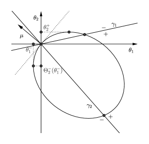
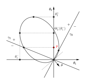
Refer to caption
Refer to caption
Refer to caption
Refer to caption
Figure 9: On the left μ1<0subscript𝜇10\mu_{1}<0 and μ2>0subscript𝜇20\mu_{2}>0, and on the right μ1>0subscript𝜇10\mu_{1}>0 and μ2<0subscript𝜇20\mu_{2}<0. The figures on the top represent the ellipses γ=0𝛾0\gamma=0, and the figures on the bottom show the domains 𝒢subscript𝒢\mathcal{G}_{\mathcal{R}} and related quantities. Recall that the drift is orthogonal to the tangent at the origin of the ellipse. Remark that contrary to the doubly negative drift case, the real point Θ2±(θ1)superscriptsubscriptΘ2plus-or-minussuperscriptsubscript𝜃1\Theta_{2}^{\pm}(\theta_{1}^{-}) of the hyperbola \mathcal{R} may now be negative

Let us also very briefly mention here the case of reflected Brownian motion in higher dimension [31, 34, 7, 6, 15]. Compared to its two-dimensional analogue, much less is known. However, an analogue of the functional equation (5) can still be stated (since the BAR exists in any dimension, see [33, 14]). Clearly, our techniques (based on complex analysis) use the dimension 222, and in our opinion, generalizing in higher dimension these BVP techniques is a difficult open problem. In the discrete case too, the case of dimension 333 is less understood. One can mention [12] for some ideas to state a BVP in dimension 333, as well as [4] for more combinatorial techniques.

4 Singularity analysis and asymptotics of the boundary distribution

The asymptotics (up to a constant) of the boundary measures has been obtained by Dai and Miyazawa in [18], see also [17, 28] for the interior measure. In this section we show that our expression (14) for the Laplace transform φ1subscript𝜑1\varphi_{1} stated in Theorem 1 is perfectly suited for singularity analysis, and accordingly to study the asymptotics (including the computation of the constant) of the boundary stationary distributions ν1subscript𝜈1\nu_{1} and ν2subscript𝜈2\nu_{2}. We shall first recall the result of [18] and express it in terms of our notations. Then we will explain how, thanks to Theorem 1, we could obtain a new proof of this result and make the constants explicit.

4.1 Asymptotic results

Theorem 16 (Theorem 6.1 of [18]).

Under the assumption (15), the following asymptotics holds:

limxν1(x)xκeτ2x=b,subscript𝑥subscript𝜈1𝑥superscript𝑥𝜅superscript𝑒subscript𝜏2𝑥𝑏\lim_{x\to\infty}\frac{\nu_{1}(x)}{x^{\kappa}e^{-\tau_{2}x}}=b, (41)

where κ{32,12,0,1}𝜅321201\kappa\in\{-\frac{3}{2},-\frac{1}{2},0,1\} and τ2{p,p,θ2+}subscript𝜏2𝑝superscript𝑝superscriptsubscript𝜃2\tau_{2}\in\{p,p^{\prime},\theta_{2}^{+}\} are given in Table 1, and b𝑏b is some positive constant. See Figures 10 and 11 to visualize geometrically the different cases.

We now propose a series of three remarks on Theorem 16.

\bullet We have already introduced p𝑝p, see (18), and psuperscript𝑝p^{\prime} is as follows: it is the (unique, when it exists) non-zero point p=Θ2+(r)superscript𝑝superscriptsubscriptΘ2𝑟p^{\prime}=\Theta_{2}^{+}(r), with r𝑟r defined by γ2(r,Θ2(r))=0subscript𝛾2𝑟superscriptsubscriptΘ2𝑟0\gamma_{2}(r,\Theta_{2}^{-}(r))=0 and rΘ1±(θ2+)𝑟superscriptsubscriptΘ1plus-or-minussuperscriptsubscript𝜃2r\leqslant\Theta_{1}^{\pm}(\theta_{2}^{+}). It will be convenient to adopt the following notation: we will write p>θ2+𝑝superscriptsubscript𝜃2p>\theta_{2}^{+} (resp. p>θ2+superscript𝑝superscriptsubscript𝜃2p^{\prime}>\theta_{2}^{+}) when p𝑝p (resp. psuperscript𝑝p^{\prime}) does not exist.

\bullet Theorem 6.1 of [18] deals with the asymptotics of ν1(x,)subscript𝜈1𝑥\nu_{1}(x,\infty), and not with that of ν1(x)subscript𝜈1𝑥\nu_{1}(x), as stated in Theorem 16 below. However, the two statements are equivalent: when the asymptotics of the density has the form bxκeτ2x𝑏superscript𝑥𝜅superscript𝑒subscript𝜏2𝑥bx^{\kappa}e^{-\tau_{2}x} as in (41), the corresponding tail probability is given by the exact same asymptotics (with another constant b𝑏b), see [17, Lemma D.5].

\bullet Before stating Table 1, which gives the values of κ𝜅\kappa and τ2subscript𝜏2\tau_{2} of Theorem 16, we briefly recall Dai and Miyazawa’s notations: θ(2,max)superscript𝜃2\theta^{(2,\max)} is the (unique) point of the ellipse γ=0𝛾0\gamma=0 such that θ2(2,max)=θ2+superscriptsubscript𝜃22superscriptsubscript𝜃2\theta_{2}^{(2,\max)}=\theta_{2}^{+}, τ2=sup{θ2>0:θ1,φ(θ1,θ2)<}subscript𝜏2supremumconditional-setsubscript𝜃20formulae-sequencesubscript𝜃1𝜑subscript𝜃1subscript𝜃2\tau_{2}=\sup\{\theta_{2}>0:\exists\theta_{1}\in\mathbb{R},\varphi(\theta_{1},\theta_{2})<\infty\} and θ(2,r)superscript𝜃2𝑟\theta^{(2,r)} is the intersection point of the straight line γ1=0subscript𝛾10\gamma_{1}=0 and the ellipse γ=0𝛾0\gamma=0. Notice that the definition of τ2subscript𝜏2\tau_{2} does not rely on an analytic continuation of φ𝜑\varphi.

Cases Dai and Miyazawa’s categories κ𝜅\kappa τ2subscript𝜏2\tau_{2}
p𝑝p or p(0,θ2+)superscript𝑝0superscriptsubscript𝜃2p^{\prime}\in(0,\theta_{2}^{+}) 1.a p<Θ2(θ1)𝑝superscriptsubscriptΘ2superscriptsuperscriptsubscript𝜃1absent\displaystyle p<\Theta_{2}^{-}(\theta_{1}^{-})^{\phantom{{}^{\prime}}} τ2<θ2(2,max)subscript𝜏2superscriptsubscript𝜃22\tau_{2}<\theta_{2}^{(2,\max)} Categories I or I​I 00 p𝑝p
1.b Θ2(θ1)p<psuperscriptsubscriptΘ2superscriptsubscript𝜃1𝑝superscriptsuperscript𝑝absent\Theta_{2}^{-}(\theta_{1}^{-})\leqslant p<{p^{\prime}}^{\phantom{{}^{\prime}}} Category I 00 p𝑝p
1.c Θ2(θ1)p<psuperscriptsubscriptΘ2superscriptsubscript𝜃1superscript𝑝𝑝\Theta_{2}^{-}(\theta_{1}^{-})\leqslant p^{\prime}<p Category I​I​I, τ2θ2(2,r)subscript𝜏2superscriptsuperscriptsubscript𝜃22𝑟absent\tau_{2}\neq{\theta_{2}^{(2,r)}}^{\phantom{{}^{\prime}}} 00 psuperscript𝑝p^{\prime}
1.d Θ2(θ1)p=psuperscriptsubscriptΘ2superscriptsubscript𝜃1𝑝superscript𝑝\Theta_{2}^{-}(\theta_{1}^{-})\leqslant p=p^{\prime} Category I​I​I, τ2=θ2(2,r)subscript𝜏2superscriptsubscript𝜃22𝑟\tau_{2}=\theta_{2}^{(2,r)} 111 p𝑝p
p𝑝p and pθ2+superscript𝑝superscriptsubscript𝜃2p^{\prime}\geqslant\theta_{2}^{+} 2.a p𝑝p and p>θ2+superscript𝑝superscriptsubscript𝜃2p^{\prime}>\theta_{2}^{+} τ2=θ2(2,max)subscript𝜏2superscriptsubscript𝜃22\tau_{2}=\theta_{2}^{(2,\max)} Category I, θ(2,r)θ(2,max)superscript𝜃2𝑟superscriptsuperscript𝜃2absent\theta^{(2,r)}\neq{\theta^{(2,\max)}}^{\phantom{{}^{\prime}}} 3232-\frac{3}{2} θ2+superscriptsubscript𝜃2\theta_{2}^{+}
2.b θ2+=psuperscriptsubscript𝜃2superscript𝑝absent\theta_{2}^{+}=p^{\phantom{{}^{\prime}}} Category I, θ(2,r)=θ(2,max)superscript𝜃2𝑟superscriptsuperscript𝜃2absent\theta^{(2,r)}={\theta^{(2,\max)}}^{\phantom{{}^{\prime}}} 1212-\frac{1}{2} θ2+superscriptsubscript𝜃2\theta_{2}^{+}
2.c θ2+=psuperscriptsubscript𝜃2superscriptsuperscript𝑝absent\theta_{2}^{+}={p^{\prime}}^{\phantom{{}^{\prime}}} Category I​I, θ(2,r)θ(2,max)superscript𝜃2𝑟superscriptsuperscript𝜃2absent\theta^{(2,r)}\neq{\theta^{(2,\max)}}^{\phantom{{}^{\prime}}} 1212-\frac{1}{2} θ2+superscriptsubscript𝜃2\theta_{2}^{+}
2.d θ2+=p=psuperscriptsubscript𝜃2𝑝superscriptsuperscript𝑝absent\theta_{2}^{+}=p={p^{\prime}}^{\phantom{{}^{\prime}}} Category I​I, θ(2,r)=θ(2,max)superscript𝜃2𝑟superscriptsuperscript𝜃2absent\theta^{(2,r)}={\theta^{(2,\max)}}^{\phantom{{}^{\prime}}} 00 θ2+superscriptsubscript𝜃2\theta_{2}^{+}
Table 1: Dai and Miyazawa’s categories expressed with our notations
Refer to caption
Refer to caption
Refer to caption
Refer to caption
Refer to caption
Refer to caption
Refer to caption
Refer to caption
Figure 10: Ellipses and curves in the cases 1.a, 1.b, 1.c and 1.d of Table 1
Refer to caption
Refer to caption
Refer to caption
Refer to caption
Figure 11: Ellipses in the cases 2.a, 2.b, 2.c and 2.d of Table 1

4.2 Sketch of the proof of Theorem 16

The idea is to study the singularities of φ1subscript𝜑1\varphi_{1} and to use transfer theorems (such as [20, Theorem 37.1]) relating the asymptotics of a function and the singularities of its Laplace transform. In our case, the singularity closest to 00 will determine the asymptotics. Our aim here is not to propose a complete proof of Theorem 16 (for this we refer to [18]), but rather to illustrate that Theorem 1 indeed implies Theorem 16, with the additional feature of providing an exact expression for the constant b𝑏b in (41). We give details for the case 1.a of Table 1, and only sketch the difficulties that would arise in the remaining cases.

Proof of Theorem 16 and computation of b𝑏b in case 1.a.

In that case, the index χ𝜒\chi equals 11-1 and the formula (14) gives

φ1(θ2)=ν1(+)(w(0)w(p)w(θ2)w(p))exp{12iπlogG(θ)[w(θ)w(θ)w(θ2)w(θ)w(θ)w(0)]dθ}.subscript𝜑1subscript𝜃2subscript𝜈1subscript𝑤0𝑤𝑝𝑤subscript𝜃2𝑤𝑝12𝑖𝜋subscriptsuperscript𝐺𝜃delimited-[]superscript𝑤𝜃𝑤𝜃𝑤subscript𝜃2superscript𝑤𝜃𝑤𝜃𝑤0differential-d𝜃\varphi_{1}(\theta_{2})=\\ \nu_{1}(\mathbb{R}_{+})\left(\frac{w(0)-w(p)}{w(\theta_{2})-w(p)}\right)\exp\bigg{\{}\frac{1}{2i\pi}\int_{\mathcal{R}^{-}}\log G(\theta)\left[\frac{w^{\prime}(\theta)}{w(\theta)-w(\theta_{2})}-\frac{w^{\prime}(\theta)}{w(\theta)-w(0)}\right]\mathrm{d}\theta\bigg{\}}.

Recall that w𝑤w is analytic, one-to-one on 𝒢subscript𝒢\mathcal{G}_{\mathcal{R}} and further satisfies w(θ2)w(θ)𝑤subscript𝜃2𝑤𝜃w(\theta_{2})\neq w(\theta), for all θ2𝒢subscript𝜃2subscript𝒢\theta_{2}\in\mathcal{G}_{\mathcal{R}} and θ𝜃superscript\theta\in\mathcal{R}^{-}. As a first result, the integral part (thus also its exponential) is analytic in the domain 𝒢subscript𝒢\mathcal{G}_{\mathcal{R}}. A second consequence is that 1w(θ2)w(p)1𝑤subscript𝜃2𝑤𝑝\frac{1}{w(\theta_{2})-w(p)} has a simple pole at p𝑝p: φ1(θ2)=b+o(1)θ2p,subscript𝜑1subscript𝜃2𝑏𝑜1subscript𝜃2𝑝\varphi_{1}(\theta_{2})=\frac{b+o(1)}{\theta_{2}-p}, with

b=ν1(+)(w(0)w(p)w(p))exp{12iπlogG(θ)[w(θ)w(θ)w(p)w(θ)w(θ)w(0)]dθ}.𝑏subscript𝜈1subscript𝑤0𝑤𝑝superscript𝑤𝑝12𝑖𝜋subscriptsuperscript𝐺𝜃delimited-[]superscript𝑤𝜃𝑤𝜃𝑤𝑝superscript𝑤𝜃𝑤𝜃𝑤0differential-d𝜃b=\nu_{1}(\mathbb{R}_{+})\left(\frac{w(0)-w(p)}{w^{\prime}(p)}\right)\exp\bigg{\{}\frac{1}{2i\pi}\int_{\mathcal{R}^{-}}\log G(\theta)\left[\frac{w^{\prime}(\theta)}{w(\theta)-w(p)}-\frac{w^{\prime}(\theta)}{w(\theta)-w(0)}\right]\mathrm{d}\theta\bigg{\}}.

Theorem 37.1 of [20] gives the announced asymptotics ν1(x)=epx(b+o(1))subscript𝜈1𝑥superscript𝑒𝑝𝑥𝑏𝑜1\nu_{1}(x)=e^{-px}(b+o(1)) as x𝑥x\to\infty. ∎

In the other cases, the singularities are not in 𝒢subscript𝒢\mathcal{G}_{\mathcal{R}} and we thus need to extend meromorphically φ1subscript𝜑1\varphi_{1} in a larger domain:

Proposition 17 (Theorem 11 of [28]).

The Laplace transform φ1subscript𝜑1\varphi_{1} can be meromorphically continued on the domain [θ2+,)superscriptsubscript𝜃2\mathbb{C}\setminus[\theta_{2}^{+},\infty).

Proposition 17 has already been proved in [28], see Theorem 11 there. Note that the formula (14) of Theorem 1 provides an alternative, direct, analytic proof, which can be sketched as follows: the equation (14) is valid a priori only for θ2subscript𝜃2\theta_{2} in 𝒢subscript𝒢\mathcal{G}_{\mathcal{R}}. However, considering a Hankel contour similar to that of Figure 12, surrounding [θ2+,)superscriptsubscript𝜃2[\theta_{2}^{+},\infty), we could write φ1subscript𝜑1\varphi_{1} as an integral over the cut [θ2+,)superscriptsubscript𝜃2[\theta_{2}^{+},\infty). The study of the so-obtained formula would give the singularities p𝑝p, psuperscript𝑝p^{\prime} and θ2+superscriptsubscript𝜃2\theta_{2}^{+} as in Table 1, and would lead to the precise asymptotics (we could even obtain the full asymptotic development) and the computation of b𝑏b.

Remark 18.

We have already commented on the fact that within a single formula, Theorem 1 actually captures two different expressions, depending on the value of χ𝜒\chi in (34). From an asymptotic viewpoint, Section 4 shows that different cases exist as well, depending on various parameters. It should be noted that these cases are all different, i.e., d𝑑{d} and χ𝜒\chi do not govern the asymptotic behavior of the boundary measures.

4.3 Asymptotics at 00 of the boundary densities

Let us introduce the key parameter

α=ε+δπβ,𝛼𝜀𝛿𝜋𝛽\alpha=\frac{\varepsilon+\delta-\pi}{\beta}, (42)

where ε𝜀\varepsilon and δ𝛿\delta are the reflection angles defined in Appendix A. They are in (0,π)0𝜋(0,\pi) and satisfy

tanε=sinβr21r11σ11σ22+cosβandtanδ=sinβr12r22σ22σ11+cosβ.formulae-sequence𝜀𝛽subscript𝑟21subscript𝑟11subscript𝜎11subscript𝜎22𝛽and𝛿𝛽subscript𝑟12subscript𝑟22subscript𝜎22subscript𝜎11𝛽\tan\varepsilon=\frac{\sin\beta}{\frac{r_{21}}{r_{11}}\sqrt{\frac{\sigma_{11}}{\sigma_{22}}}+\cos\beta}\qquad\text{and}\qquad\tan\delta=\frac{\sin\beta}{\frac{r_{12}}{r_{22}}\sqrt{\frac{\sigma_{22}}{\sigma_{11}}}+\cos\beta}. (43)

The quantity α𝛼\alpha is constantly used in the literature to establish some criteria. For example, α<1𝛼1\alpha<1 if and only if the semimartingale reflected Brownian motion exists, see [57]. See also [40] for a recent paper on the case α(1,2)𝛼12\alpha\in(1,2).

As we shall prove now, the exponent in the asymptotics at \infty of φ1subscript𝜑1\varphi_{1} is directly related to this crucial parameter of the model:

Proposition 19.

Let α𝛼\alpha be defined in (42). There exists a positive constant C>0𝐶0C>0 such that

φ1(θ2)θ2Cθ2α1.subscript𝜑1subscript𝜃2subscript𝜃2similar-to𝐶superscriptsubscript𝜃2𝛼1\varphi_{1}(\theta_{2})\underset{\theta_{2}\to\infty}{\sim}C\theta_{2}^{\alpha-1}. (44)

Before proving (44), let us explain informally how the previous result should be related to the asymptotics of the stationary distribution at 00.

Remark 20.

Combined to the functional equation (4), Proposition 19 and its analogue for φ2(θ1)subscript𝜑2subscript𝜃1\varphi_{2}(\theta_{1}) lead to, for any s[0,]𝑠0s\in[0,\infty],

φ(θ1,θ2)θ1,θ2θ2/θ1sCs(θ12+θ22)α22,𝜑subscript𝜃1subscript𝜃2FRACOPsubscript𝜃1subscript𝜃2subscript𝜃2subscript𝜃1𝑠similar-tosubscript𝐶𝑠superscriptsuperscriptsubscript𝜃12superscriptsubscript𝜃22𝛼22\varphi(\theta_{1},\theta_{2})\underset{\theta_{1},\theta_{2}\to\infty\atop\theta_{2}/\theta_{1}\to s}{\sim}C_{s}\bigl{(}\theta_{1}^{2}+\theta_{2}^{2}\bigr{)}^{\frac{\alpha-2}{2}}, (45)

for some constant Cs>0subscript𝐶𝑠0C_{s}>0. Moreover, classical transfer theorems connect singularities and asymptotics of a function and its (inverse) Laplace transform. The latter suggest that (44) and (45) might be transferred as (below, (r,t)𝑟𝑡(r,t) represent the polar coordinates of (x1,x2)subscript𝑥1subscript𝑥2(x_{1},x_{2}))

ν1(x2)x20Cx2αandπ(x1,x2)=π(rcost,rsint)r0Ctrαsubscript𝜈1subscript𝑥2subscript𝑥20similar-to𝐶superscriptsubscript𝑥2𝛼and𝜋subscript𝑥1subscript𝑥2𝜋𝑟𝑡𝑟𝑡𝑟0similar-tosubscript𝐶𝑡superscript𝑟𝛼\nu_{1}(x_{2})\underset{x_{2}\to 0}{\sim}Cx_{2}^{-\alpha}\qquad\text{and}\qquad\pi(x_{1},x_{2})=\pi(r\cos t,r\sin t)\underset{r\to 0}{\sim}C_{t}r^{-\alpha}

for positive constants C𝐶C and Ctsubscript𝐶𝑡C_{t}.

The above equation is reminiscent of the following (non-asymptotic) formula [56]

π(rcost,rsint)=rαsin(δαt)𝜋𝑟𝑡𝑟𝑡superscript𝑟𝛼𝛿𝛼𝑡{\pi}(r\cos t,r\sin t)=r^{-\alpha}\sin(\delta-\alpha t)

obtained in the driftless case, for r>0𝑟0r>0 and t[0,β]𝑡0𝛽t\in[0,\beta], and where δ𝛿\delta is the reflection angle defined in (43). It means that the density π𝜋\pi behaves near the corner as in the driftless case. As explained in [35], a probabilistic interpretation is that the behavior at the corner is determined on the small scale where the drift may be neglected compared to the Brownian part.

Let us finally remark that these formulas are consistent with the fact that the process reaches the boundary if α>0𝛼0\alpha>0 (see [55, 56]); indeed, in this case the stationary distribution goes to infinity near the corner.

Proof of Proposition 19.

First of all, let us recall that we have defined ψ1subscript𝜓1\psi_{1} such that

φ1(θ2)=ψ1(W(θ2)),subscript𝜑1subscript𝜃2subscript𝜓1𝑊subscript𝜃2\varphi_{1}(\theta_{2})=\psi_{1}(W(\theta_{2})),

see (28), where for some q𝒢𝑞subscript𝒢q\in\mathbb{R}\in\mathcal{G}_{\mathcal{R}},

W(θ2)=w(θ2)+1w(θ2)w(q),𝑊subscript𝜃2𝑤subscript𝜃21𝑤subscript𝜃2𝑤𝑞W(\theta_{2})=\frac{w(\theta_{2})+1}{w(\theta_{2})-w(q)},

see (27). In the rest of the proof, C𝐶C will denote a non-zero constant that may differ from line to line.

The formulas (36) and (38) entail that

ψ1(t)t1C(t1)d+Δ2πχ.subscript𝜓1𝑡𝑡1similar-to𝐶superscript𝑡1𝑑Δ2𝜋𝜒\psi_{1}(t)\underset{t\to 1}{\sim}C(t-1)^{\frac{{d}+\Delta}{2\pi}-\chi}.

Moreover, by (33) we have

tand+Δ2=detRdetΣσ12(r11r22+r12r21)σ22r11r12σ11r22r21,𝑑Δ2𝑅Σsubscript𝜎12subscript𝑟11subscript𝑟22subscript𝑟12subscript𝑟21subscript𝜎22subscript𝑟11subscript𝑟12subscript𝜎11subscript𝑟22subscript𝑟21\tan\frac{{d}+\Delta}{2}=\frac{\det R\sqrt{\det\Sigma}}{\sigma_{12}(r_{11}r_{22}+r_{12}r_{21})-\sigma_{22}r_{11}r_{12}-\sigma_{11}r_{22}r_{21}},

and by (31), χ=d+Δ2π𝜒𝑑Δ2𝜋\chi=\lfloor\frac{{d}+\Delta}{2\pi}\rfloor. Further, by (10) and (12), w(θ2)θ2Cθ2πβ𝑤subscript𝜃2subscript𝜃2similar-to𝐶superscriptsubscript𝜃2𝜋𝛽w(\theta_{2})\underset{\theta_{2}\to\infty}{\sim}C{\theta_{2}^{\frac{\pi}{\beta}}}, thus W(θ2)1θ2Cθ2πβ𝑊subscript𝜃21subscript𝜃2similar-to𝐶superscriptsubscript𝜃2𝜋𝛽W(\theta_{2})-1\underset{\theta_{2}\to\infty}{\sim}C{\theta_{2}^{-\frac{\pi}{\beta}}}. We deduce that

φ1(θ2)θ2Cθ2d+Δ2β+χπβ.subscript𝜑1subscript𝜃2subscript𝜃2similar-to𝐶superscriptsubscript𝜃2𝑑Δ2𝛽𝜒𝜋𝛽\varphi_{1}(\theta_{2})\underset{\theta_{2}\to\infty}{\sim}C\theta_{2}^{-\frac{{d}+\Delta}{2\beta}+\chi\frac{\pi}{\beta}}.

Using now (47) and (11) gives that

tan(ε+δβ)=tand+Δ2.𝜀𝛿𝛽𝑑Δ2\tan(\varepsilon+\delta-\beta)=-\tan\frac{{d}+\Delta}{2}.

Combined with the fact that d+Δ2(π,π)𝑑Δ2𝜋𝜋\frac{{d}+\Delta}{2}\in(-\pi,\pi) and 0<ε+δβ<π0𝜀𝛿𝛽𝜋0<\varepsilon+\delta-\beta<\pi (due to the recurrence condition and α<1𝛼1\alpha<1), this implies

d+Δ2={ε+δβπ if d+Δ>0, i.e., if χ=0,ε+δβ if d+Δ<0, i.e., if χ=1,𝑑Δ2cases𝜀𝛿𝛽𝜋formulae-sequence if 𝑑Δ0 i.e., if 𝜒0𝜀𝛿𝛽formulae-sequence if 𝑑Δ0 i.e., if 𝜒1-\frac{{d}+\Delta}{2}=\begin{cases}\varepsilon+\delta-\beta-\pi&\text{ if }{d}+\Delta>0,\text{ i.e., if }\chi=0,\\ \varepsilon+\delta-\beta&\text{ if }{d}+\Delta<0,\text{ i.e., if }\chi=-1,\end{cases}

which means

d+Δ2=ε+δβπχπ.𝑑Δ2𝜀𝛿𝛽𝜋𝜒𝜋-\frac{{d}+\Delta}{2}=\varepsilon+\delta-\beta-\pi-\chi\pi.

We deduce that

φ1(θ2)θ2Cθ2α1.subscript𝜑1subscript𝜃2subscript𝜃2similar-to𝐶superscriptsubscript𝜃2𝛼1\varphi_{1}(\theta_{2})\underset{\theta_{2}\to\infty}{\sim}C\theta_{2}^{\alpha-1}.\qed

5 Algebraic nature and simplification of the Laplace transforms

Motivations

In this section we are interested in the following question: in which extent is it possible to simplify the expressions of the Laplace transforms given in Theorem 1? For instance, is this possible that these functions be algebraic or even rational?

This is of paramount importance: first, simplified expressions would lead to an easier analysis, in particular for asymptotic analysis or for taking inverse Laplace transforms; second, understanding the parameters (Σ,μ,R)Σ𝜇𝑅(\Sigma,\mu,R) for which the Laplace transforms are rational should reveal intrinsic structure of the model. In the particular case of the identity covariance matrix ΣΣ\Sigma, some attempts of simplifications may be found in [26, Chapter 4].

In the literature, this question has received much interest in the discrete setting. One can first think at the famous Jackson’s networks [36] and their product form solutions. In a closer context, Latouche and Miyazawa [41], Chen, Boucherie and Goseling [10], obtain geometric necessary and sufficient conditions for the stationary distribution of random walks in the quarter plane to be sums of geometric terms. Such criteria can be applied, e.g., to derive an approximation scheme to error bounds for performance measures of random walks in the quarter plane [11].

In our context of reflected diffusions in the quadrant, analogues of these results are obtained by Dieker and Moriarty [19]: a simple condition (involving the single angle (46)) for the stationary density to be a sum of exponential terms is derived. We will discuss the links with our results in Section 5.1. In the simplest case the sum of exponential terms consist of one single term: this is the skew-symmetric condition (24) of [34]. In this case, a factorization such as in Remark 8 exists and applying an invariant method we are able to solve the skew-symmetric case, see our Section 5.2, yielding new proofs to already known results.

Another main reason which can lead to simplified expressions comes from the rationality of βπ𝛽𝜋\frac{\beta}{\pi}, with β𝛽\beta in (11). Before being more precise, let us mention that this reason is deeply different than the first one: β𝛽\beta only depends on the covariance matrix and is therefore independent of the reflection matrix, while Dieker and Moriarty’s condition is also dependent on the reflection angles, see (46). In the discrete setting, the rationality of βπ𝛽𝜋\frac{\beta}{\pi} is rather interpreted as a condition on the finiteness of a certain group of transformations, and this finiteness was shown to have a decisive influence on the D-finiteness (a function is D-finite if it satisfies a linear differential equation with polynomial coefficients on \mathbb{Q}) of the generating functions, see [25, 5, 21]. For reflected Brownian motion in the quadrant with orthogonal reflections, it is shown in [29] that the Laplace transform is algebraic (note, any algebraic function is D-finite) if and only if the group is finite. We present a structural result in Section 5.3.

Finally, we focus in Section 5.4 on the case of orthogonal reflections, and derive a new proof of the main result of [29], as a consequence of Theorem 1.

5.1 Dieker and Moriarty’s criterion

For the sake of completeness, let us mention the following result:

Theorem 21 (Theorem 1 in [19]).

The stationary density is a sum of exponentials if and only if

α=ε+δπβ={0,1,2,},𝛼𝜀𝛿𝜋𝛽012{\color[rgb]{0,0,0}\alpha=\frac{\varepsilon+\delta-\pi}{\beta}}\in-\mathbb{N}=-\{0,1,2,\ldots\}, (46)

with ε𝜀\varepsilon and δ𝛿\delta in (0,π)0𝜋(0,\pi) and

tanε=sinβr21r11σ11σ22+cosβ,tanδ=sinβr12r22σ22σ11+cosβ.formulae-sequence𝜀𝛽subscript𝑟21subscript𝑟11subscript𝜎11subscript𝜎22𝛽𝛿𝛽subscript𝑟12subscript𝑟22subscript𝜎22subscript𝜎11𝛽\tan\varepsilon=\frac{\sin\beta}{\frac{r_{21}}{r_{11}}\sqrt{\frac{\sigma_{11}}{\sigma_{22}}}+\cos\beta},\qquad\tan\delta=\frac{\sin\beta}{\frac{r_{12}}{r_{22}}\sqrt{\frac{\sigma_{22}}{\sigma_{11}}}+\cos\beta}. (47)

Notice that this is not the exact statement of [19, Theorem 1], as in Dieker and Moriarty’s paper, the Brownian motion is assumed to have an identity covariance matrix and evolves in a wedge with an arbitrary opening angle, whereas we consider Brownian motion with arbitrary covariance matrix but in the quarter plane. A simple linear transform, which is made explicit in Appendix A, makes both statements equivalent. The expression (47) of the angles ε𝜀\varepsilon and δ𝛿\delta follows from this transformation.

5.2 Skew-symmetric case

The skew-symmetric case holds when the matrix condition (24) is satisfied [34]. In dimension two, (24) can be reduced to the single equation

2σ12=r21r11σ11+r12r22σ22.2subscript𝜎12subscript𝑟21subscript𝑟11subscript𝜎11subscript𝑟12subscript𝑟22subscript𝜎222\sigma_{12}=\frac{r_{21}}{r_{11}}\sigma_{11}+\frac{r_{12}}{r_{22}}\sigma_{22}. (48)

Using the identities in (55) we easily show that the above condition is equivalent to

ε+δ=π,𝜀𝛿𝜋\varepsilon+\delta=\pi,

which is the case where the quantity α𝛼\alpha of Dieker and Moriarty’s criterion is equal to 00, see (46).

It is known, see [34], that condition (24) is satisfied if and only if the stationary distribution has a product form, i.e., π(x1,x2)=π2(x1)π1(x2)𝜋subscript𝑥1subscript𝑥2subscript𝜋2subscript𝑥1subscript𝜋1subscript𝑥2\pi(x_{1},x_{2})=\pi_{2}(x_{1})\pi_{1}(x_{2}), where the πisubscript𝜋𝑖\pi_{i}’s are the marginal densities of π𝜋\pi. Furthermore it implies that the stationary distribution is exponential, meaning that

π(x1,x2)=ζ1ζ2eζ1x1ζ2x2,with (ζ1ζ2)=2diag(Σ)1diag(R)R1μ.formulae-sequence𝜋subscript𝑥1subscript𝑥2subscript𝜁1subscript𝜁2superscript𝑒subscript𝜁1subscript𝑥1subscript𝜁2subscript𝑥2with subscript𝜁1subscript𝜁22diagsuperscriptΣ1diag𝑅superscript𝑅1𝜇\pi(x_{1},x_{2})=\zeta_{1}\zeta_{2}e^{-\zeta_{1}x_{1}-\zeta_{2}x_{2}},\quad\text{with }\small\left(\begin{array}[]{l}\zeta_{1}\\ \zeta_{2}\end{array}\right)=-2\cdot\text{diag}(\Sigma)^{-1}\cdot\text{diag}(R)\cdot R^{-1}\cdot\mu. (49)

See for example [31, §10], [34] or [18] for more details on these results.

In fact, in the skew-symmetric case, a rational factorization such as in the Remark 8 exists. It is then possible to find again, in another way, some already known results. Indeed if the skew-symmetric condition holds, we shall prove below that for θ2subscript𝜃2\theta_{2}\in\mathcal{R},

G(θ2)=F(θ2)F(θ2¯),with F(θ2)=ζ2θ2.formulae-sequence𝐺subscript𝜃2𝐹subscript𝜃2𝐹¯subscript𝜃2with 𝐹subscript𝜃2subscript𝜁2subscript𝜃2G(\theta_{2})=\frac{F(\theta_{2})}{F(\overline{\theta_{2}})},\quad\text{with }F(\theta_{2})=\zeta_{2}-\theta_{2}. (50)

where by (49) ζ2subscript𝜁2\zeta_{2} takes the value

ζ2=2r22(r21μ1r11μ2)σ22detR.subscript𝜁22subscript𝑟22subscript𝑟21subscript𝜇1subscript𝑟11subscript𝜇2subscript𝜎22𝑅\zeta_{2}=\frac{2r_{22}(r_{21}\mu_{1}-r_{11}\mu_{2})}{\sigma_{22}\det R}. (51)

Using (48) and (19) it is easy to remark that ζ2=psubscript𝜁2𝑝\zeta_{2}=p, which is the only possible pole of φ1subscript𝜑1\varphi_{1} in 𝒢subscript𝒢\mathcal{G}_{\mathcal{R}} as we observe after Lemma 3. It follows from Proposition 6 that the function φ1(θ2)(ζ2θ2)subscript𝜑1subscript𝜃2subscript𝜁2subscript𝜃2\varphi_{1}(\theta_{2})(\zeta_{2}-\theta_{2})

  • is bounded on 𝒢subscript𝒢\mathcal{G}_{\mathcal{R}} and converges at infinity to ν1(0)subscript𝜈10\nu_{1}(0) (thanks to the initial value theorem and Lemma 3),

  • is continuous on 𝒢¯¯subscript𝒢\overline{\mathcal{G}_{\mathcal{R}}},

  • satisfies the boundary condition φ1(θ2)(ζ2θ2)=φ1(θ2¯)(ζ2θ2¯)subscript𝜑1subscript𝜃2subscript𝜁2subscript𝜃2subscript𝜑1¯subscript𝜃2subscript𝜁2¯subscript𝜃2\varphi_{1}(\theta_{2})(\zeta_{2}-\theta_{2})=\varphi_{1}(\overline{\theta_{2}})(\zeta_{2}-\overline{\theta_{2}}) for all θ2subscript𝜃2\theta_{2}\in\mathcal{R}.

Then, using an invariant lemma (see Lemma 2 in [44, Section 10.2]), we conclude that for some constant C𝐶C,

φ1(θ2)=Cζ2θ2.subscript𝜑1subscript𝜃2𝐶subscript𝜁2subscript𝜃2\varphi_{1}(\theta_{2})=\frac{C}{\zeta_{2}-\theta_{2}}.

Evaluating the above equation at 00 and using Lemma 15 gives C=σ112r11ζ1ζ2𝐶subscript𝜎112subscript𝑟11subscript𝜁1subscript𝜁2C=\frac{\sigma_{11}}{2r_{11}}\zeta_{1}\zeta_{2}. Inverting the Laplace transform implies that the stationary distribution is exponential. Then using the functional equation (5), we find that σ11σ224r11r22ζ1ζ2φ(θ1,θ2)=φ1(θ2)φ2(θ1)subscript𝜎11subscript𝜎224subscript𝑟11subscript𝑟22subscript𝜁1subscript𝜁2𝜑subscript𝜃1subscript𝜃2subscript𝜑1subscript𝜃2subscript𝜑2subscript𝜃1\frac{\sigma_{11}\sigma_{22}}{4r_{11}r_{22}}\zeta_{1}\zeta_{2}\varphi(\theta_{1},\theta_{2})=\varphi_{1}(\theta_{2})\varphi_{2}(\theta_{1}), which means that π𝜋\pi has a product form.

Proof of Equation (50).

Let θ2subscript𝜃2\theta_{2}\in\mathcal{R} and note θ1=Θ1(θ2)subscript𝜃1superscriptsubscriptΘ1subscript𝜃2\theta_{1}=\Theta_{1}^{-}(\theta_{2}). Elementary computations give

γ1(θ1,θ2)γ2(θ1,θ2¯)=θ1(2r22σ22(r21μ1r11μ2)θ2detR).subscript𝛾1subscript𝜃1subscript𝜃2subscript𝛾2subscript𝜃1¯subscript𝜃2subscript𝜃12subscript𝑟22subscript𝜎22subscript𝑟21subscript𝜇1subscript𝑟11subscript𝜇2subscript𝜃2𝑅\gamma_{1}(\theta_{1},\theta_{2})\gamma_{2}(\theta_{1},\overline{\theta_{2}})=\theta_{1}\left(\frac{2r_{22}}{\sigma_{22}}(r_{21}\mu_{1}-r_{11}\mu_{2})-\theta_{2}\det R\right).

To find this, we just have to use the skew-symmetric condition (48) and to remark that for θ2subscript𝜃2\theta_{2}\in\mathcal{R} Vieta’s formulas give θ2θ2¯=1σ22(σ11θ12+2μ1θ1)subscript𝜃2¯subscript𝜃21subscript𝜎22subscript𝜎11superscriptsubscript𝜃122subscript𝜇1subscript𝜃1\theta_{2}\overline{\theta_{2}}=\frac{1}{\sigma_{2}2}(\sigma_{11}\theta_{1}^{2}+2\mu_{1}\theta_{1}) and θ2¯=θ21σ22(2σ12θ1+2μ2)¯subscript𝜃2subscript𝜃21subscript𝜎222subscript𝜎12subscript𝜃12subscript𝜇2\overline{\theta_{2}}=-\theta_{2}-\frac{1}{\sigma_{22}}(2\sigma_{12}\theta_{1}+2\mu_{2}). Then, using the expression (51) of ζ2subscript𝜁2\zeta_{2} we find G(θ2)=ζ2θ2ζ2θ2¯𝐺subscript𝜃2subscript𝜁2subscript𝜃2subscript𝜁2¯subscript𝜃2G(\theta_{2})=\frac{\zeta_{2}-\theta_{2}}{\zeta_{2}-\overline{\theta_{2}}} for θ2subscript𝜃2\theta_{2}\in\mathcal{R}. ∎

5.3 Structural form of the Laplace transforms

In the case βπ𝛽𝜋\frac{\beta}{\pi}\in\mathbb{Q}, and in this case only, the function W𝑊W in (27) is algebraic (as the generalized Chebyshev polynomial (10) is, see Remark 10), yielding the following structural result:

Proposition 22.

If βπ𝛽𝜋\frac{\beta}{\pi}\in\mathbb{Q}, the Laplace transform φ1subscript𝜑1\varphi_{1} of Theorem 1 is the product of an algebraic function by the exponential of a D-finite function.

Proof.

This easily follows from the fact that the Cauchy integral of a D-finite function is D-finite, see, e.g., [52]. ∎

However, it is not true in general that the exponential of a D-finite function is still D-finite.

5.4 Orthogonal reflections

Here we consider the case of orthogonal reflections, which is equivalent for the reflection matrix R𝑅R in (1) to be the identity matrix; see also Figure 2. By developing the theory of Tutte’s invariants (introduced by Tutte in [54] for the enumeration of properly colored triangulations, and used in [3] for the enumeration of quadrant walks) for the Brownian motion, we proved in [29] the following result:

Theorem 23 (Theorem 1 in [29]).

Let R𝑅R be the identity matrix in (1). The Laplace transform φ1subscript𝜑1\varphi_{1} is equal to

φ1(θ2)=μ1w(0)w(θ2)w(0)θ2.subscript𝜑1subscript𝜃2subscript𝜇1superscript𝑤0𝑤subscript𝜃2𝑤0subscript𝜃2\varphi_{1}(\theta_{2})=\frac{-\mu_{1}w^{\prime}(0)}{w(\theta_{2})-w(0)}\theta_{2}. (52)

In this section we derive a new proof of this result, as a consequence of Theorem 1. More generally, the proof below would work for any parameters (Σ,μ,R)Σ𝜇𝑅(\Sigma,\mu,R) such that G(θ2)=F(θ2)F(θ2¯)𝐺subscript𝜃2𝐹subscript𝜃2𝐹¯subscript𝜃2G(\theta_{2})=\frac{F(\theta_{2})}{F(\overline{\theta_{2}})} (cf. Remark 8), yielding a rational expression of φ1(θ2)subscript𝜑1subscript𝜃2\varphi_{1}(\theta_{2}) in terms of w(θ2)𝑤subscript𝜃2w(\theta_{2}) and θ2subscript𝜃2\theta_{2}.

Proof.

Let us first notice that the index χ=0𝜒0\chi=0. Indeed, since G(θ2)=θ2¯θ2𝐺subscript𝜃2¯subscript𝜃2subscript𝜃2G(\theta_{2})=\frac{\overline{\theta_{2}}}{\theta_{2}}, we have argG(θ2)=2argθ2>0𝐺subscript𝜃22subscript𝜃20\arg G(\theta_{2})=-2\arg\theta_{2}>0 for θ2subscript𝜃2\theta_{2}\in\mathcal{R}, and thus Δ>0Δ0\Delta>0, see the proof of Lemma 14.

Starting from the formula (40), we have for some constant C𝐶C

φ1(θ2)=Cexp{12iπ(logθ¯logθ)W(θ)W(θ)W(θ2)dθ}=Cexp{12iπlogθW(θ)W(θ)W(θ2)dθ}.subscript𝜑1subscript𝜃2𝐶12𝑖𝜋subscriptsuperscript¯𝜃𝜃superscript𝑊𝜃𝑊𝜃𝑊subscript𝜃2differential-d𝜃𝐶12𝑖𝜋subscript𝜃superscript𝑊𝜃𝑊𝜃𝑊subscript𝜃2d𝜃\varphi_{1}(\theta_{2})=C\exp\bigg{\{}{\frac{1}{2i\pi}\int_{\mathcal{R}^{-}}(\log\overline{\theta}-\log\theta)\frac{W^{\prime}(\theta)}{W(\theta)-W(\theta_{2})}\mathrm{d}\theta}\bigg{\}}=C\exp\bigg{\{}{\frac{1}{2i\pi}\int_{\mathcal{R}}\log\theta\frac{W^{\prime}(\theta)}{W(\theta)-W(\theta_{2})}\mathrm{d}\theta}\bigg{\}}.

To compute the above integral, we first integrate on the contour represented on Figure 12. The residue theorem gives

12iπ{R+𝒞R+𝒞ε+R+iεiε+iεRiε}logθW(θ)W(θ)W(θ2)dθ=logθ2logq.12𝑖𝜋subscriptsubscript𝑅subscriptsubscript𝒞𝑅subscriptsubscript𝒞𝜀superscriptsubscript𝑅𝑖𝜀𝑖𝜀superscriptsubscript𝑖𝜀𝑅𝑖𝜀𝜃superscript𝑊𝜃𝑊𝜃𝑊subscript𝜃2d𝜃subscript𝜃2𝑞\frac{1}{2i\pi}\bigg{\{}\int_{\mathcal{R}_{R}}+\int_{\mathcal{C}_{R}}+\int_{\mathcal{C}_{\varepsilon}}+\int_{-R+i\varepsilon}^{i\varepsilon}+\int_{-i\varepsilon}^{-R-i\varepsilon}\bigg{\}}\log\theta\frac{W^{\prime}(\theta)}{W(\theta)-W(\theta_{2})}\mathrm{d}\theta=\log\theta_{2}-\log q. (53)
Refer to caption
Figure 12: Integration contour used in the proof of Theorem 23

It is easy to see that

limR12iπRlogθW(θ)W(θ)W(θ2)dθ=12iπlogθW(θ)W(θ)W(θ2)dθsubscript𝑅12𝑖𝜋subscriptsubscript𝑅𝜃superscript𝑊𝜃𝑊𝜃𝑊subscript𝜃2d𝜃12𝑖𝜋subscript𝜃superscript𝑊𝜃𝑊𝜃𝑊subscript𝜃2d𝜃\lim_{R\to\infty}\frac{1}{2i\pi}\int_{\mathcal{R}_{R}}\log\theta\frac{W^{\prime}(\theta)}{W(\theta)-W(\theta_{2})}\mathrm{d}\theta=\frac{1}{2i\pi}\int_{\mathcal{R}}\log\theta\frac{W^{\prime}(\theta)}{W(\theta)-W(\theta_{2})}\mathrm{d}\theta

and that in the limits when ε0𝜀0\varepsilon\to 0 and R𝑅R\to\infty, the contributions on 𝒞εsubscript𝒞𝜀\mathcal{C}_{\varepsilon} and 𝒞Rsubscript𝒞𝑅\mathcal{C}_{R} both converge to 00, because W𝑊W is analytic at 00 and \infty, respectively.

Furthermore,

limε0limR12iπ{R+iεiε+iεRiε}subscript𝜀0subscript𝑅12𝑖𝜋superscriptsubscript𝑅𝑖𝜀𝑖𝜀superscriptsubscript𝑖𝜀𝑅𝑖𝜀\displaystyle\lim_{\varepsilon\to 0}\lim_{R\to\infty}\frac{1}{2i\pi}\bigg{\{}\int_{-R+i\varepsilon}^{i\varepsilon}+\int_{-i\varepsilon}^{-R-i\varepsilon}\bigg{\}} logθW(θ)W(θ)W(θ2)dθ𝜃superscript𝑊𝜃𝑊𝜃𝑊subscript𝜃2d𝜃\displaystyle\log\theta\frac{W^{\prime}(\theta)}{W(\theta)-W(\theta_{2})}\mathrm{d}\theta
=limε012iπ0(log(t+iε)log(tiε))W(θ)W(θ)W(θ2)dθabsentsubscript𝜀012𝑖𝜋superscriptsubscript0𝑡𝑖𝜀𝑡𝑖𝜀superscript𝑊𝜃𝑊𝜃𝑊subscript𝜃2differential-d𝜃\displaystyle=\lim_{\varepsilon\to 0}\frac{1}{2i\pi}\int_{-\infty}^{0}(\log(t+i\varepsilon)-\log(t-i\varepsilon))\frac{W^{\prime}(\theta)}{W(\theta)-W(\theta_{2})}\mathrm{d}\theta
=12iπ02iπW(θ)W(θ)W(θ2)dθabsent12𝑖𝜋superscriptsubscript02𝑖𝜋superscript𝑊𝜃𝑊𝜃𝑊subscript𝜃2differential-d𝜃\displaystyle=\frac{1}{2i\pi}\int_{-\infty}^{0}2i\pi\frac{W^{\prime}(\theta)}{W(\theta)-W(\theta_{2})}\mathrm{d}\theta
=logW(0)W(θ2)W()W(θ2)absent𝑊0𝑊subscript𝜃2𝑊𝑊subscript𝜃2\displaystyle=\log\frac{W(0)-W(\theta_{2})}{W(\infty)-W(\theta_{2})}
=logw(θ2)w(0)w(q)w(0).absent𝑤subscript𝜃2𝑤0𝑤𝑞𝑤0\displaystyle=\log\frac{w(\theta_{2})-w(0)}{w(q)-w(0)}.

Above we have used the dominated convergence and the fact that the principal determination of the logarithm gives us limε0(log(t+iε)log(tiε))=2iπsubscript𝜀0𝑡𝑖𝜀𝑡𝑖𝜀2𝑖𝜋\lim_{\varepsilon\to 0}(\log(t+i\varepsilon)-\log(t-i\varepsilon))=2i\pi. Letting R𝑅R\to\infty and then ε0𝜀0\varepsilon\to 0 in (53), we have, for some constants C𝐶C and Csuperscript𝐶C^{\prime},

φ1(θ2)=Cexp{12iπlogθW(θ)W(θ)W(θ2)dθ}=Cθ2w(θ2)w(0).subscript𝜑1subscript𝜃2𝐶12𝑖𝜋subscript𝜃superscript𝑊𝜃𝑊𝜃𝑊subscript𝜃2d𝜃superscript𝐶subscript𝜃2𝑤subscript𝜃2𝑤0\varphi_{1}(\theta_{2})=C\exp\bigg{\{}\frac{1}{2i\pi}\int_{\mathcal{R}}\log\theta\frac{W^{\prime}(\theta)}{W(\theta)-W(\theta_{2})}\mathrm{d}\theta\bigg{\}}=C^{\prime}\frac{\theta_{2}}{w(\theta_{2})-w(0)}.

Since by Lemma 15 one has φ1(0)=μ1subscript𝜑10subscript𝜇1\varphi_{1}(0)=-\mu_{1}, this eventually gives the right constant in (52). ∎

Appendix A Equivalence between Brownian motion in wedges and Brownian motion in the quarter plane

We use the notation of Section 1. Up to an isomorphism, studying Brownian motion in the quarter plane with arbitrary covariance matrix ΣΣ\Sigma is equivalent to studying Brownian motion in a cone of angle β=arccosσ12σ11σ22𝛽subscript𝜎12subscript𝜎11subscript𝜎22\beta=\arccos-\frac{\sigma_{12}}{\sqrt{\sigma_{11}\sigma_{22}}}, with covariance identity. See for example [1, Equation (23)] and [50, Lemma 3.23]. In this short section we relate the key parameters (angles of the reflection vectors and drift) before and after the linear transformation.

Let us define the linear transforms

T=(1sinβcotβ01)(1σ11001σ22),T1=(σ1100σ22)(sinβcosβ01).formulae-sequence𝑇matrix1𝛽𝛽01matrix1subscript𝜎11001subscript𝜎22superscript𝑇1matrixsubscript𝜎1100subscript𝜎22matrix𝛽𝛽01T=\begin{pmatrix}\frac{1}{\sin\beta}&\cot\beta\\ 0&1\end{pmatrix}\begin{pmatrix}\frac{1}{\sqrt{\sigma_{11}}}&0\\ 0&\frac{1}{\sqrt{\sigma_{22}}}\end{pmatrix},\qquad T^{-1}=\begin{pmatrix}\sqrt{\sigma_{11}}&0\\ 0&\sqrt{\sigma_{22}}\end{pmatrix}\begin{pmatrix}\sin\beta&-{\cos\beta}\\ 0&\phantom{-}1\end{pmatrix}. (54)
Refer to caption
Refer to caption
Figure 13: The linear transformation T𝑇T in (54) from the quadrant to the wedge of opening angle β𝛽\beta

Obviously the reflected Brownian motion associated to (Σ,μ,R)Σ𝜇𝑅(\Sigma,\mu,R) becomes a Brownian motion (with covariance identity) in a wedge of angle β𝛽\beta and with parameters (Id,Tμ,TR)Id𝑇𝜇𝑇𝑅(\text{Id},T\mu,TR). The new angles of reflection are δ𝛿\delta and ε𝜀\varepsilon (cf. Figure 13), such that

{tanδ=sinβa+cosβ,cosδ=a+cosβa2+2acosβ+1,sinδ=sinβa2+2acosβ+1,tanε=sinβb+cosβ,cosε=b+cosβb2+2bcosβ+1,sinε=sinβb2+2bcosβ+1,cases𝛿𝛽𝑎𝛽𝛿𝑎𝛽superscript𝑎22𝑎𝛽1𝛿𝛽superscript𝑎22𝑎𝛽1𝜀𝛽𝑏𝛽𝜀𝑏𝛽superscript𝑏22𝑏𝛽1𝜀𝛽superscript𝑏22𝑏𝛽1\left\{\begin{array}[]{lll}\tan\delta=\dfrac{\sin\beta}{a+\cos\beta},&\quad\cos\delta=\dfrac{a+\cos\beta}{\sqrt{a^{2}+2a\cos\beta+1}},&\quad\sin\delta=\dfrac{\sin\beta}{\sqrt{a^{2}+2a\cos\beta+1}},\vskip 3.0pt plus 1.0pt minus 1.0pt\vskip 3.0pt plus 1.0pt minus 1.0pt\\ \tan\varepsilon=\dfrac{\sin\beta}{b+\cos\beta},&\quad\cos\varepsilon=\dfrac{b+\cos\beta}{\sqrt{b^{2}+2b\cos\beta+1}},&\quad\sin\varepsilon=\dfrac{\sin\beta}{\sqrt{b^{2}+2b\cos\beta+1}},\end{array}\right. (55)

where a=r12r22σ22σ11𝑎subscript𝑟12subscript𝑟22subscript𝜎22subscript𝜎11a=\frac{r_{12}}{r_{22}}\sqrt{\frac{\sigma_{22}}{\sigma_{11}}} and b=r21r11σ11σ22𝑏subscript𝑟21subscript𝑟11subscript𝜎11subscript𝜎22b=\frac{r_{21}}{r_{11}}\sqrt{\frac{\sigma_{11}}{\sigma_{22}}}. The new drift is μ~=Tμ~𝜇𝑇𝜇\widetilde{\mu}=T\mu, where

μ~1=μ1σ111sinβ+μ2σ22cotβ and μ~2=μ2σ22.formulae-sequencesubscript~𝜇1subscript𝜇1subscript𝜎111𝛽subscript𝜇2subscript𝜎22𝛽 and subscript~𝜇2subscript𝜇2subscript𝜎22\widetilde{\mu}_{1}=\frac{\mu_{1}}{\sqrt{\sigma_{11}}}\frac{1}{\sin\beta}+\frac{\mu_{2}}{\sqrt{\sigma_{22}}}\cot\beta\quad\text{ and }\quad\widetilde{\mu}_{2}=\frac{\mu_{2}}{\sqrt{\sigma_{22}}}.

To conclude the appendix, we prove Corollary 2, which gives an explicit formula for the Laplace transform of the stationary distribution of a reflected Brownian motion in a wedge.

Proof of Corollary 2.

Let us arbitrarily choose σ11=σ22=1subscript𝜎11subscript𝜎221\sigma_{11}=\sigma_{22}=1 and σ12=cosβsubscript𝜎12𝛽\sigma_{12}=-\cos\beta. It implies that the linear transform T𝑇T in (54) is the same as T1subscript𝑇1T_{1} in the statement of Corollary 2. We consider the process Z=T1Z~𝑍superscript𝑇1~𝑍Z=T^{-1}\widetilde{Z}, which is a reflected Brownian motion in the quadrant of parameters (Σ,μ,R)Σ𝜇𝑅(\Sigma,\mu,R), with

Σ=T1Σ~(T1),μ=T1μ~andR=T1R~.formulae-sequenceΣsuperscript𝑇1~Σsuperscriptsuperscript𝑇1topformulae-sequence𝜇superscript𝑇1~𝜇and𝑅superscript𝑇1~𝑅\Sigma=T^{-1}\widetilde{\Sigma}(T^{-1})^{\top},\quad\mu=T^{-1}\widetilde{\mu}\quad\text{and}\quad R=T^{-1}\widetilde{R}.

Let ΠΠ\Pi (resp. Π~~Π\widetilde{\Pi}) be the invariant measure of Z𝑍Z (resp. Z~~𝑍\widetilde{Z}) and π𝜋\pi (resp. π~~𝜋\widetilde{\pi}) its density. It is easy to notice that

Π=Π~Tandπ=|detT|π~T.formulae-sequenceΠ~Π𝑇and𝜋𝑇~𝜋𝑇\Pi=\widetilde{\Pi}\circ T\quad\text{and}\quad\pi=|\det T|\widetilde{\pi}\circ T.

Indeed, by a fundamental property of the invariant measure, for all x+2𝑥superscriptsubscript2x\in\mathbb{R}_{+}^{2} and all measurable set A𝐴A in +2superscriptsubscript2\mathbb{R}_{+}^{2} we have the following limits

x[ZtA]tΠ(A),x[ZtA]=x[TZtTA]=Tx[Z~tTA]tΠ~(TA).subscript𝑥delimited-[]subscript𝑍𝑡𝐴𝑡Π𝐴subscript𝑥delimited-[]subscript𝑍𝑡𝐴subscript𝑥delimited-[]𝑇subscript𝑍𝑡𝑇𝐴subscript𝑇𝑥delimited-[]subscript~𝑍𝑡𝑇𝐴𝑡~Π𝑇𝐴\mathbb{P}_{x}[Z_{t}\in A]\underset{t\to\infty}{\longrightarrow}\Pi(A),\qquad\mathbb{P}_{x}[Z_{t}\in A]=\mathbb{P}_{x}[TZ_{t}\in TA]=\mathbb{P}_{Tx}[\widetilde{Z}_{t}\in TA]\underset{t\to\infty}{\longrightarrow}\widetilde{\Pi}(TA).

It yields Π=Π~TΠ~Π𝑇\Pi=\widetilde{\Pi}\circ T. Furthermore by a simple change of variable we have

Π~T(A)=TAπ~(x~)dx~=|detT|Aπ~(Tx)dx,~Π𝑇𝐴subscript𝑇𝐴~𝜋~𝑥differential-d~𝑥𝑇subscript𝐴~𝜋𝑇𝑥differential-d𝑥\widetilde{\Pi}\circ T(A)=\int_{TA}\widetilde{\pi}(\widetilde{x})\mathrm{d}\widetilde{x}=|\det T|\int_{A}\widetilde{\pi}(Tx)\mathrm{d}x,

therefore |detT|π~T𝑇~𝜋𝑇|\det T|\widetilde{\pi}\circ T is the density of ΠTΠ𝑇\Pi\circ T and is then equal to π𝜋\pi. Theorem 1 gives the value of φ𝜑\varphi, the Laplace transform of π𝜋\pi. Lastly, a simple change of variable x~=Tx~𝑥𝑇𝑥\widetilde{x}=Tx in Equation (3) leads to

φ~(θ~)=𝒞βexp(θ~x~)π~(x~)dx~=T1𝒞βexp(θ~Tx)π~(Tx)|detT|dx=+2exp(Tθ~x)π(x)dx=φ(Tθ~),~𝜑~𝜃subscriptdouble-integralsubscript𝒞𝛽~𝜃~𝑥~𝜋~𝑥differential-d~𝑥subscriptdouble-integralsuperscript𝑇1subscript𝒞𝛽~𝜃𝑇𝑥~𝜋𝑇𝑥𝑇differential-d𝑥subscriptdouble-integralsuperscriptsubscript2superscript𝑇top~𝜃𝑥𝜋𝑥differential-d𝑥𝜑superscript𝑇top~𝜃\widetilde{\varphi}(\widetilde{\theta})=\iint_{\mathcal{C}_{\beta}}\exp(\widetilde{\theta}\cdot\widetilde{x})\widetilde{\pi}(\widetilde{x})\mathrm{d}\widetilde{x}=\iint_{T^{-1}\mathcal{C}_{\beta}}\exp(\widetilde{\theta}\cdot Tx)\widetilde{\pi}(Tx)|\det T|\mathrm{d}x=\iint_{\mathbb{R}_{+}^{2}}\exp(T^{\top}\widetilde{\theta}\cdot x)\pi(x)\mathrm{d}x=\varphi(T^{\top}\widetilde{\theta}),

where 𝒞βsubscript𝒞𝛽\mathcal{C}_{\beta} is the wedge of angle β𝛽\beta where the process evolves. ∎

References

  • Aspandiiarov et al., [1996] Aspandiiarov, S., Iasnogorodski, R., and Menshikov, M. (1996). Passage-time moments for nonnegative stochastic processes and an application to reflected random walks in a quadrant. Ann. Probab., 24(2):932–960.
  • Baccelli and Fayolle, [1987] Baccelli, F. and Fayolle, G. (1987). Analysis of models reducible to a class of diffusion processes in the positive quarter plane. SIAM J. Appl. Math., 47(6):1367–1385.
  • Bernardi et al., [2016] Bernardi, O., Bousquet-Mélou, M., and Raschel, K. (2016). Counting quadrant walks via Tutte’s invariant method. In Proceedings of FPSAC 2016, Discrete Math. Theor. Comput. Sci. Proc., pages 203–214. Assoc. Discrete Math. Theor. Comput. Sci., Nancy.
  • Bostan et al., [2016] Bostan, A., Bousquet-Mélou, M., Kauers, M., and Melczer, S. (2016). On 3-dimensional lattice walks confined to the positive octant. Ann. Comb., 20(4):661–704.
  • Bousquet-Mélou and Mishna, [2010] Bousquet-Mélou, M. and Mishna, M. (2010). Walks with small steps in the quarter plane. In Algorithmic probability and combinatorics, volume 520 of Contemp. Math., pages 1–39. Amer. Math. Soc., Providence, RI.
  • Bramson, [2011] Bramson, M. (2011). Positive recurrence for reflecting Brownian motion in higher dimensions. Queueing Syst., 69(3-4):203–215.
  • Bramson et al., [2010] Bramson, M., Dai, J., and Harrison, J. (2010). Positive recurrence of reflecting Brownian motion in three dimensions. Ann. Appl. Probab., 20(2):753–783.
  • Burdzy et al., [2017] Burdzy, K., Chen, Z.-Q., Marshall, D., and Ramanan, K. (2017). Obliquely reflected Brownian motion in non-smooth planar domains. Ann. Probab., 45(5):2971–3037.
  • Chen, [1996] Chen, H. (1996). A sufficient condition for the positive recurrence of a semimartingale reflecting Brownian motion in an orthant. Ann. Appl. Probab., 6(3):758–765.
  • Chen et al., [2015] Chen, Y., Boucherie, R., and Goseling, J. (2015). The invariant measure of random walks in the quarter-plane: representation in geometric terms. Probab. Engrg. Inform. Sci., 29(2):233–251.
  • Chen et al., [2016] Chen, Y., Boucherie, R., and Goseling, J. (2016). Invariant measures and error bounds for random walks in the quarter-plane based on sums of geometric terms. Queueing Syst., 84(1-2):21–48.
  • Cohen, [1984] Cohen, J. (1984). On a functional relation in three complex variables; three coupled processors. Technical Report Mathematical Institute Utrecht 359, Utrecht University.
  • Dai, [1990] Dai, J. (1990). Steady-state analysis of reflected Brownian motions: Characterization, numerical methods and queueing applications. ProQuest LLC, Ann Arbor, MI. Thesis (Ph.D.)–Stanford University.
  • Dai and Harrison, [1992] Dai, J. and Harrison, J. (1992). Reflected Brownian motion in an orthant: numerical methods for steady-state analysis. Ann. Appl. Probab., 2(1):65–86.
  • Dai and Harrison, [2012] Dai, J. and Harrison, J. (2012). Reflecting Brownian motion in three dimensions: a new proof of sufficient conditions for positive recurrence. Math. Methods Oper. Res., 75(2):135–147.
  • Dai and Kurtz, [1994] Dai, J. and Kurtz, T. (1994). Characterization of the stationary distribution for a semimartingale reflecting brownian motion in a convex polyhedron. Preprint, pages 1–31.
  • Dai and Miyazawa, [2011] Dai, J. and Miyazawa, M. (2011). Reflecting Brownian motion in two dimensions: Exact asymptotics for the stationary distribution. Stoch. Syst., 1(1):146–208.
  • Dai and Miyazawa, [2013] Dai, J. and Miyazawa, M. (2013). Stationary distribution of a two-dimensional SRBM: geometric views and boundary measures. Queueing Syst., 74(2-3):181–217.
  • Dieker and Moriarty, [2009] Dieker, A. and Moriarty, J. (2009). Reflected Brownian motion in a wedge: sum-of-exponential stationary densities. Electron. Commun. Probab., 14:1–16.
  • Doetsch, [1974] Doetsch, G. (1974). Introduction to the Theory and Application of the Laplace Transformation. Springer Berlin Heidelberg, Berlin, Heidelberg.
  • Dreyfus et al., [2018] Dreyfus, T., Hardouin, C., Roques, J., and Singer, M. F. (2018). On the nature of the generating series of walks in the quarter plane. Invent. Math., 213(1):139–203.
  • Dubédat, [2004] Dubédat, J. (2004). Reflected planar Brownian motions, intertwining relations and crossing probabilities. Ann. Inst. H. Poincaré Probab. Statist., 40(5):539–552.
  • Dupuis and Williams, [1994] Dupuis, P. and Williams, R. (1994). Lyapunov functions for semimartingale reflecting Brownian motions. Ann. Probab., 22(2):680–702.
  • Fayolle and Iasnogorodski, [1979] Fayolle, G. and Iasnogorodski, R. (1979). Two coupled processors: the reduction to a Riemann-Hilbert problem. Z. Wahrsch. Verw. Gebiete, 47(3):325–351.
  • Fayolle et al., [1999] Fayolle, G., Iasnogorodski, R., and Malyshev, V. (1999). Random Walks in the Quarter-Plane. Springer Berlin Heidelberg, Berlin, Heidelberg.
  • Foddy, [1984] Foddy, M. (1984). Analysis of Brownian motion with drift, confined to a quadrant by oblique reflection (diffusions, Riemann-Hilbert problem). ProQuest LLC, Ann Arbor, MI. Thesis (Ph.D.)–Stanford University.
  • Foschini, [1982] Foschini, G. (1982). Equilibria for diffusion models of pairs of communicating computers—symmetric case. IEEE Trans. Inform. Theory, 28(2):273–284.
  • Franceschi and Kurkova, [2017] Franceschi, S. and Kurkova, I. (2017). Asymptotic expansion for the stationary distribution of a reflected brownian motion in the quarter plane. Stoch. Syst., 7(1):32–94.
  • Franceschi and Raschel, [2017] Franceschi, S. and Raschel, K. (2017). Tutte’s invariant approach for Brownian motion reflected in the quadrant. ESAIM Probab. Stat., 21:220–234.
  • Harrison and Hasenbein, [2009] Harrison, J. and Hasenbein, J. (2009). Reflected Brownian motion in the quadrant: tail behavior of the stationary distribution. Queueing Syst., 61(2-3):113–138.
  • [31] Harrison, J. and Reiman, M. (1981a). On the distribution of multidimensional reflected Brownian motion. SIAM J. Appl. Math., 41(2):345–361.
  • [32] Harrison, J. and Reiman, M. (1981b). Reflected Brownian motion on an orthant. Ann. Probab., 9(2):302–308.
  • [33] Harrison, J. and Williams, R. (1987a). Brownian models of open queueing networks with homogeneous customer populations. Stochastics, 22(2):77–115.
  • [34] Harrison, J. and Williams, R. (1987b). Multidimensional reflected Brownian motions having exponential stationary distributions. Ann. Probab., 15(1):115–137.
  • Hobson and Rogers, [1993] Hobson, D. and Rogers, L. (1993). Recurrence and transience of reflecting Brownian motion in the quadrant. In Mathematical Proceedings of the Cambridge Philosophical Society, volume 113, pages 387–399. Cambridge Univ Press.
  • Jackson, [1957] Jackson, J. (1957). Networks of waiting lines. Operations Res., 5:518–521.
  • Kella and Ramasubramanian, [2012] Kella, O. and Ramasubramanian, S. (2012). Asymptotic irrelevance of initial conditions for Skorohod reflection mapping on the nonnegative orthant. Math. Oper. Res., 37(2):301–312.
  • Kella and Whitt, [1996] Kella, O. and Whitt, W. (1996). Stability and structural properties of stochastic storage networks. J. Appl. Probab., 33(4):1169–1180.
  • Kurkova and Suhov, [2003] Kurkova, I. and Suhov, Y. (2003). Malyshev’s theory and JS-queues. Asymptotics of stationary probabilities. Ann. Appl. Probab., 13(4):1313–1354.
  • Lakner et al., [2016] Lakner, P., Reed, J., and Zwart, B. (2016). A Dirichlet process characterization of RBM in a wedge. Preprint arXiv:1605.02020, pages 1–37.
  • Latouche and Miyazawa, [2014] Latouche, G. and Miyazawa, M. (2014). Product-form characterization for a two-dimensional reflecting random walk. Queueing Syst., 77(4):373–391.
  • Le Gall, [1987] Le Gall, J.-F. (1987). Mouvement brownien, cônes et processus stables. Probab. Theory Related Fields, 76(4):587–627.
  • Lépingle, [2017] Lépingle, D. (2017). A two-dimensional oblique extension of Bessel processes. Markov Process. Related Fields, 23(4):233–266.
  • Litvinchuk, [2000] Litvinchuk, G. (2000). Solvability Theory of Boundary Value Problems and Singular Integral Equations with Shift. Springer Netherlands, Dordrecht.
  • Malyšev, [1972] Malyšev, V. (1972). An analytic method in the theory of two-dimensional positive random walks. Sibirsk. Mat. Ž., 13:1314–1329, 1421.
  • Muskhelishvili, [1972] Muskhelishvili, N. (1972). Singular integral equations. Wolters-Noordhoff Publishing, Groningen. Boundary problems of functions theory and their applications to mathematical physics, Revised translation from the Russian, edited by J. R. M. Radok, Reprinted.
  • O’Connell and Ortmann, [2014] O’Connell, N. and Ortmann, J. (2014). Product-form invariant measures for brownian motion with drift satisfying a skew-symmetry type condition. ALEA, Lat. Am. J. Probab. Math. Stat., 11(1):307–329.
  • Reiman and Williams, [1988] Reiman, M. and Williams, R. (1988). A boundary property of semimartingale reflecting Brownian motions. Probab. Theory Related Fields, 77(1):87–97.
  • Sarantsev, [2013] Sarantsev, A. (2013). Comparison techniques for competing brownian particles. Preprint arXiv:1305.1653, pages 1–31.
  • Sarantsev, [2015] Sarantsev, A. (2015). Triple and simultaneous collisions of competing Brownian particles. Electron. J. Probab., 20:no. 29, 28.
  • Sarantsev, [2017] Sarantsev, A. (2017). Reflected Brownian motion in a convex polyhedral cone: tail estimates for the stationary distribution. J. Theoret. Probab., 30(3):1200–1223.
  • Takayama, [1992] Takayama, N. (1992). An approach to the zero recognition problem by Buchberger algorithm. J. Symbolic Comput., 14(2-3):265–282.
  • Taylor and Williams, [1993] Taylor, L. and Williams, R. (1993). Existence and uniqueness of semimartingale reflecting Brownian motions in an orthant. Probab. Theory Related Fields, 96(3):283–317.
  • Tutte, [1995] Tutte, W. (1995). Chromatic sums revisited. Aequationes Math., 50(1-2):95–134.
  • Varadhan and Williams, [1985] Varadhan, S. and Williams, R. (1985). Brownian motion in a wedge with oblique reflection. Comm. Pure Appl. Math., 38(4):405–443.
  • [56] Williams, R. (1985a). Recurrence classification and invariant measure for reflected Brownian motion in a wedge. Ann. Probab., 13(3):758–778.
  • [57] Williams, R. (1985b). Reflected Brownian motion in a wedge: semimartingale property. Z. Wahrsch. Verw. Gebiete, 69(2):161–176.
  • Williams, [1995] Williams, R. (1995). Semimartingale reflecting Brownian motions in the orthant. In Stochastic networks, volume 71 of IMA Vol. Math. Appl., pages 125–137. Springer, New York.