Nucleon spin structure functions at NNLO in the presence of target mass corrections and higher twist effects

Abstract

We extract polarized parton distribution functions (PPDFs), referred to as “KTA17,” together with the highly correlated strong coupling $\alpha_{s}$ from recent and up-to-date $g_{1}$ and $g_{2}$ polarized structure functions world data at next-to-next-to-leading order in perturbative QCD. The stability and reliability of the results are ensured by including nonperturbative target mass corrections as well as higher-twist terms which are particularly important at the large-$x$ region at low Q². Their role in extracting the PPDFs in the nucleon is studied. Sum rules are discussed and compared with other results from the literature. This analysis is made by means of the Jacobi polynomials expansion technique to the DGLAP evolution. The uncertainties on the observables and on the PPDFs throughout this paper are computed using standard Hessian error propagation which served to provide a more realistic estimate of the PPDFs uncertainties.

I Introduction

Hadrons are the complex systems consisting of quarks and gluons. The determination of parton densities and understanding the details of their $x$ and $Q^{2}$ dependence is one of the most important challenges in high energy physics. A straightforward calculation of the cross section is available via the collinear factorization theorem in perturbative QCD (pQCD). Particularly interesting is the investigation of polarized processes which provides information about the basic decomposition of nucleon’s spin into its quark and gluon constituent parts. In recent years, the deep inelastic scattering (DIS) of polarized leptons off polarized nucleons has played an important role in the study of the nucleon spin structure functions. The spin structure of the nucleon is still one of the major unresolved issues in the study related to hadronic physics Aidala:2012mv . While the combined quark and antiquark spin contributions to the nucleon spin, have been measured to be about 30%, the contribution of the gluon spin to the spin of the nucleon is still insufficiently constrained after more than two decades of intense study. The last few years have witnessed tremendous experimental and phenomenological progress in our understanding on the spin structure of the nucleon. There are several QCD analyses of the polarized DIS data along with the estimation of their uncertainties in the literature Ball:2016spl ; deFlorian:2009vb ; Hirai:2008aj ; Blumlein:2010rn ; Leader:2010rb ; Nocera:2014gqa ; Jimenez-Delgado:2013boa ; Jimenez-Delgado:2014xza ; Sato:2016tuz ; Arbabifar:2013tma ; Monfared:2014nta ; Shahri:2016uzl ; Gluck:2000dy .

Current phenomenological spin-dependent parton distribution function (PDF) analysis uses the spin-dependent DIS measurements on $g_{1}^{\rm p,n,d}(x,Q^{2})$ and $g_{2}^{\rm p,n,d}(x,Q^{2})$, see Table 1. Beside these data sets, one can also include the recent PHENIX measurement on neutral-pion $\pi^{0}$ productions Adare:2014hsq ; Adare:2015ozj at $\sqrt{s}=200,\,510$ GeV and inclusive jet production from the STAR Collaboration Adamczyk:2014ozi in polarized proton-proton collisions at the Relativistic Heavy Ion Collider (RHIC). The longitudinal single-spin asymmetries in $W^{\pm}$ weak boson production Adamczyk:2014xyw ; Adare:2015gsd from polarized proton-proton collisions also can be used. These data sets may lead to better determination of the polarized gluon, sea quark and antiquarks distributions at small-$x$.

The precision of polarized parton distribution functions (PPDFs) determination in QCD analyses has steadily improved over the recent years, mainly due to refined theory predictions for the hard parton scattering reactions and also more accurate experimental observables. Recently, the COMPASS Collaboration at CERN Adolph:2015saz extracted the spin-dependent structure function of the proton $g_{1}^{p}(x,Q^{2})$ and the longitudinal double-spin asymmetries $A_{1}^{p}(x,Q^{2})$ from scattering of polarized muons off polarized protons for the region of low $x$ (down to $0.0025$) and high photon virtuality $Q^{2}$. Although significant progress has been made, the gluon polarization, as a fundamental ingredient describing the inner structure of the nucleon, suffers from large uncertainties and remains poorly constrained. Worse even, the gluon distributions originating from different collaborations represent significant differences.

In our latest analysis TKAA16 Shahri:2016uzl , we performed the first detailed pQCD analysis using Jacobi polynomial approach at next-to-leading-order (NLO) and next-to-next-to-leading-order (NNLO) approximation. All the available and up-to-date $g_{1}^{\rm p,n,d}(x,Q^{2})$ world data including recent COMPASS measurements Adolph:2015saz were considered which led to new parametrization of spin-dependent parton destinies. In the discussed paper Shahri:2016uzl , we simply considered the equality of $g_{1}(x,Q^{2})\equiv g_{1}^{\tau 2}(x,Q^{2})$, while the information on quark-gluon correlation is encoded into the higher-twist parts of the $g_{1}(x,Q^{2})$ and $g_{2}(x,Q^{2})$. Here, $\tau 2$ means twist 2 and HT refers to higher twist. Although these dynamical effects are suppressed by inverse powers of $Q^{2}$ in the HT expansion of $g_{1}(x,Q^{2})$, they appear to be equally important as their twist-2 part in $g_{2}(x,Q^{2})$. This special property makes measurements of $g_{2}(x,Q^{2})$ particularly sensitive for investigating multiparton correlations in the nucleon. Furthermore, $g_{2}(x,Q^{2})$ observables are mostly in the low $Q^{2}$ region where the target mass corrections (TMCs) and HT effects become significant. In the current analysis, which we refer to as “KTA17,” we develop a precise analysis by including TMCs and HT contributions in both $g_{1}(x,Q^{2})$ and $g_{2}(x,Q^{2})$ structure functions. The role of these corrections in PPDFs estimation using pQCD fits to the data is discussed. Studies of the moments of spin-dependent structure functions provide an opportunity to test our understanding of pQCD like that of the Bjorken sum rule. We also demonstrate once more the reliability and validity of the Jacobi polynomial expansion approach at the NNLO approximation to extract the PPDFs from polarized DIS structure function.

The remainder of this article is organized as follows: In Sec. II, we review the theoretical formalism underpinning the KTA17 analysis of the polarized DIS structure function, the Jacobi polynomials approach, target mass corrections and higher-twist effects. Section III provides an overview of the method of the analysis, data selection, $\chi^{2}$ minimization and error calculation. The results of present NNLO polarized PDFs fits and detailed comparison with available observables are discussed in Sec. IV. We compute and compare associated polarized sum rules in Sec. V. A short discussion on the present status of polarized PDFs global analyses is discussed in Sec. VI. Finally, Sec. VII contains the summary and concluding remarks. In Appendix A, we present a FORTRAN package containing results for the KTA17 polarized structure functions at NNLO approximation together with corresponding uncertainties. Appendix B provides the analytical expressions for the polarized NNLO quark-quark and gluon-quark splitting functions.

II Theoretical framework

In this section, we review the basic theoretical framework for the polarized DIS structure functions on which the KTA17 PPDFs analysis is based. After a brief revision of the leading-twist structure functions at NNLO approximation, we present the Jacobi polynomials expansion method which was already used to extract KTA17 PPDFs at NNLO approximation from polarized DIS data  Shahri:2016uzl . Our approach to take into account TMCs and HT corrections is discussed in the following subsections.

II.1 Leading-twist polarized DIS structure function

In the light-cone operator-product expansion (OPE), the leading-twist (twist $\tau=2$) contributions correspond to scattering off asymptotically free partons, while the higher-twist contributions emerge due to multiparton correlations. The leading-twist spin-dependent proton and neutron structure functions, $g_{1}^{\rm p,n}(x,Q^{2})$ at NNLO, can be expressed as a linear combination of polarized parton densities and coefficient functions as Shahri:2016uzl ; Goto:1999by ; Nath:2017ofm

$$g_{1}^{\rm p}(x,Q^{2})=\frac{1}{2}\sum_{q}e^{2}_{q}\Delta q_{v}(x,Q^{2})\otimes$$

$$\left(1+\frac{\alpha_{s}(Q^{2})}{2\pi}\Delta C^{(1)}_{q}+\left(\frac{\alpha_{s}(Q^{2})}{2\pi}\right)^{2}\Delta C^{(2)}_{ns}\right)$$

$$+e^{2}_{q}(\Delta q_{s}+\Delta\bar{q_{s}})(x,Q^{2})\otimes$$

$$\left(1+\frac{\alpha_{s}(Q^{2})}{2\pi}\Delta C^{(1)}_{q}+\left(\frac{\alpha_{s}(Q^{2})}{2\pi}\right)^{2}\Delta C^{(2)}_{s}\right)$$

$$+\frac{2}{9}\Delta g(x,Q^{2})\otimes\left(\frac{\alpha_{s}(Q^{2})}{2\pi}\Delta C^{(1)}_{g}+\left(\frac{\alpha_{s}(Q^{2})}{2\pi}\right)^{2}\Delta C^{(2)}_{g}\right)$$

Here, $\Delta q_{v}$, $\Delta q_{s}$ and $\Delta g$ are the polarized valance, sea and gluon densities, respectively. The pQCD evolution kernel for PPDFs is now available at NNLO in Ref. Moch:2014sna . The $\Delta C^{(1)}_{q}$ and $\Delta C^{(1)}_{g}$ are the NLO spin-dependent quark and gluon hard scattering coefficients, calculable in pQCD Lampe:1998eu .

We applied the hard scattering coefficients extracted at NNLO approximation. In this order the Wilson coefficients are different for quarks and antiquarks and we used $\Delta C^{(2)}_{ns}$ and $\Delta C^{(2)}_{s}$ Zijlstra:1993sh . The typical convolution in $x$ space is represented with the symbol $\otimes$. Considering isospin symmetry, the corresponding neutron structure functions are available. The leading-twist deuteron structure function can be obtained from $g_{1}^{\rm p}$ and $g_{1}^{\rm n}$ via the relation

$$g_{1}^{\rm\tau 2(d)}(x,Q^{2})=\frac{1}{2}\{g_{1}^{\rm p}(x,Q^{2})+g_{1}^{\rm n}(x,Q^{2})\}\times(1-1.5w_{D})\,,$$

where $w_{D}=0.05\pm 0.01$ is the probability to find the deuteron in a $D$-state Lacombe:1981eg ; Buck:1979ff ; Zuilhof:1980ae . The leading-twist polarized structure function of $g_{2}^{\tau 2}(x,Q^{2})$ is fully determined from $g_{1}^{\tau 2}(x,Q^{2})$ via the Wandzura and Wilczek (WW) term Wandzura:1977qf ; Flay:2016wie :

$$g_{2}^{\tau 2}(x,Q^{2}) = g_{2}^{WW}(x,Q^{2})=$$ (3)

$$-g_{1}^{\tau 2}(x,Q^{2})+\int_{x}^{1}\frac{dy}{y}g_{1}^{\tau 2}(y,Q^{2})\,.$$

This relation remains valid in the leading twist even though target mass corrections are included Wandzura:1977qf .

The leading-twist definition for $g_{1}^{\tau 2}(x,Q^{2})$ and $g_{2}^{\tau 2}(x,Q^{2})$ are valid in the Bjorken limit, i.e. $Q^{2}\rightarrow\infty,\leavevmode\nobreak\ x=$ fixed. While, at a moderate low $Q^{2}$ ($\sim 1-5$ GeV²) and $W^{2}($$4$ GeV${}^{2}<W^{2}<10$ GeV²), TMCs and HT contributions should be considered completely in the nucleon structure functions studies. As we have already mentioned, the most significant improvement in KTA17 analysis in comparison to Ref. Shahri:2016uzl is the treatment of target mass corrections and higher-twist contributions to the spin-dependent structure functions. They will be discussed in detail in the following subsections.

II.2 Jacobi polynomials approach

The method we employed in this paper is based on the Jacobi polynomials expansion of the polarized structure functions. Practical aspects of this method including its major advantages are presented in our previous studies Shahri:2016uzl ; Khorramian:2010qa ; Khorramian:2009xz ; MoosaviNejad:2016ebo ; Khanpour:2016uxh and also other literature Ayala:2015epa ; Barker:1982rv ; Barker:1983iy ; Krivokhizhin:1987rz ; Krivokhizhin:1990ct ; Chyla:1986eb ; Barker:1980wu ; Kataev:1997nc ; Alekhin:1998df ; Kataev:1999bp ; Kataev:2001kk ; Kataev:2005ci ; Leader:1997kw . Here, we outline a brief review of this method. In the polynomial fitting procedure, the evolution equation is combined with the truncated series to perform a direct fit to structure functions. According to this method, one can easily expand the polarized structure functions $xg_{1}^{\rm QCD}(x,Q^{2})$, in terms of the Jacobi polynomials $\Theta_{n}^{\alpha,\beta}(x)$, as follows,

$$x\,g_{1}^{\tau 2}(x,Q^{2})=x^{\beta}(1-x)^{\alpha}\ \,\sum_{n=0}^{\rm N_{\rm max}}a_{n}(Q^{2})\,\Theta_{n}^{\alpha,\beta}(x)\,,$$ (4)

where $\rm N_{\rm max}$ is the maximum order of the expansion. The parameters $\alpha$ and $\beta$ are Jacobi polynomials free parameters which normally fixed on their best values. These parameters have to be chosen so as to achieve the fastest convergence of the series on the right-hand side of Eq. (4).

The Q² dependence of the polarized structure functions are codified in the Jacobi polynomials moments, $a_{n}(Q^{2})$. The $x$ dependence will be provided by the weight function $w^{\alpha,\beta}(x)\equiv x^{\beta}(1-x)^{\alpha}$ and the Jacobi polynomials $\Theta_{n}^{\alpha,\beta}(x)$ which can be written as,

$$\Theta_{n}^{\alpha,\beta}(x)=\sum_{j=0}^{n}\,c_{j}^{(n)}(\alpha,\beta)\,x^{j}\,,$$ (5)

where the coefficients $c_{j}^{(n)}(\alpha,\beta)$ are combinations of Gamma functions in term of $n$, $\alpha$ and $\beta$. The above Jacobi polynomials have to satisfy the following orthogonality relation,

$$\int_{0}^{1}dx\,x^{\beta}(1-x)^{\alpha}\,\Theta_{n}^{\alpha,\beta}(x)\,\Theta_{l}^{\alpha,\beta}(x)\,=\,\delta_{n,l}\,.$$ (6)

Consequently one can obtain the Jacobi moments, $a_{n}(Q^{2})$, using the above orthogonality relations as,

$$a_{n}(Q^{2}) = \int_{0}^{1}dx\,xg_{1}^{\tau 2}(x,Q^{2})\,\Theta_{n}^{\alpha,\beta}(x)$$ (7)

$$= \sum_{j=0}^{n}\,c_{j}^{(n)}(\alpha,\beta)\,{\cal M}[xg_{1}^{\tau 2},\,j+2](Q^{2})\,,$$

where the Mellin transform ${\cal{M}}[xg_{1}^{\tau 2},\rm N]$ is introduced as

$${\cal{M}}[xg_{1}^{\tau 2},{\rm N}](Q^{2})\equiv\int_{0}^{1}dx\,x^{\rm N-2}\,xg_{1}^{\tau 2}(x,Q^{2})\,.$$ (8)

Finally, having the QCD expressions for the Mellin moments ${\cal M}(Q^{2})$, we can reconstruct the polarized structure function $xg_{1}^{\tau 2}(x,Q^{2})$. Using the Jacobi polynomial expansion method, the $xg_{1}^{\tau 2}(x,Q^{2})$ can be constructed as

$$xg_{1}^{\tau 2}(x,Q^{2}) = x^{\beta}(1-x)^{\alpha}\,\sum_{n=0}^{\rm N_{max}}\,\Theta_{n}^{\alpha,\beta}(x)$$ (9)

$$\times \sum_{j=0}^{n}\,c_{j}^{(n)}{(\alpha,\beta)}\,{\cal M}[xg_{1}^{\tau 2},j+2](Q^{2})\,.$$

We have shown in our previous analyses that by setting the $N_{\rm max}$ = 9, $\alpha$ = 3, $\beta$ = 0.5, the optimal convergence of this expansion throughout the whole kinematic region constrained by the polarized DIS data is possible. If $\alpha$ is allowed to vary in the fit procedure, it takes up values close to 3 with neither a change in PPDF parameter values nor a significant improvement in the $\chi^{2}/{\rm d.o.f}$. By contrast, in the absence of sufficiently enough data to constrain $\beta$ reasonably directly, we prefer to fix $\beta$ to the value 0.5 suggested by Regge arguments at low $x$. For the chosen $\alpha$ and $\beta$ values, the rate of convergence is adequate for all practical purposes. The $\rm N_{max}$ can become arbitrarily large. The freedom to increase $\rm N_{max}$ can compensate for injudiciously chosen values of the constant $\alpha$ and $\beta$. However we want to deduce the expansion evolution terms and find the most practical form. To study the dependence of fit results to the value of $\rm N_{max}$, we also allow it to vary. In practice, we found that at $Q_{0}^{2}$ = 1 GeV², for $\alpha=3$ and $\beta=0.5$, no improvement is achieved by allowing polynomials expansion vary between seven and nine terms. Inserting the Jacobi polynomial expansion of $g_{1}^{\tau 2}(x,Q^{2})$ from Eq. (9) into the WW relation Eq. (3) leads to an analytical result for the $g_{2}^{\tau 2}(x,Q^{2})$ structure function.

II.3 Target mass corrections and threshold problem

In the low $Q^{2}$ region, the nucleon mass correction cannot be neglected and the power-suppressed corrections to the structure functions can make important contributions in some kinematic regions. Different from the case for dynamical HT effects, the TMCs can be calculated in closed-form expression. We follow the method suggested by Georgi and Politzer Georgi:1976ve in the case of the unpolarized structure function which is generalized by Blumlein and Tkabladze  Blumlein:1998nv for all polarized structure functions. These corrections were both presented in terms of the integer moments and Mellin inversion to $x$ space. The explicit twist-2 expression of $g_{1}$ with TMCs is Dong:2006jm ; Dong:2008zg ; Dong:2007iv ; Dong:2007zzc ; Sidorov:2006fi

$$g_{1}^{\rm\tau 2+TMCs}(x,Q^{2})$$ (10)

$$= \frac{xg_{1}^{\tau 2}(\xi,Q^{2};{\rm M}=0)}{\xi(1+4{\rm M}^{2}x^{2}/Q^{2})^{3/2}}$$

$$+ \frac{4{\rm M}^{2}x^{2}}{Q^{2}}\frac{(x+\xi)}{\xi(1+4{\rm M}^{2}x^{2}/Q^{2})^{2}}\int_{\xi}^{1}\frac{d\xi^{\prime}}{\xi^{\prime}}g_{1}^{\tau 2}(\xi^{\prime},Q^{2};{\rm M}=0)$$

$$- \frac{4{\rm M}^{2}x^{2}}{Q^{2}}\frac{(2-4{\rm M}^{2}x^{2}/Q^{2})}{2(1+4{\rm M}^{2}x^{2}/Q^{2})^{5/2}}$$

$$\times \int_{\xi}^{1}\frac{d\xi^{\prime}}{\xi^{\prime}}\int_{\xi^{\prime}}^{1}\frac{d\xi^{\prime\prime}}{\xi^{\prime\prime}}g_{1}^{\tau 2}(\xi^{\prime\prime},Q^{2};{\rm M}=0)\,.$$

Here, ${\rm M}$ is the nucleon mass. Similarly, the target mass corrected structure function $g_{2}$ with twist-2 contribution is given by

$$g_{2}^{\tau 2+\rm TMCs}(x,Q^{2})$$ (11)

$$= -\frac{xg_{1}^{\tau 2}(\xi,Q^{2};{\rm M}=0)}{\xi(1+4{\rm M}^{2}x^{2}/Q^{2})^{3/2}}$$

$$+ \frac{x(1-4{\rm M}^{2}x\xi/Q^{2})}{\xi(1+4{\rm M}^{2}x^{2}/Q^{2})^{2}}\int_{\xi}^{1}\frac{d\xi^{\prime}}{\xi^{\prime}}g_{1}^{\tau 2}(\xi^{\prime},Q^{2};{\rm M}=0)$$

$$+ \frac{3}{2}\frac{4{\rm M}^{2}x^{2}/Q^{2}}{(1+4{\rm M}^{2}x^{2}/Q^{2})^{5/2}}$$

$$\times \int_{\xi}^{1}\frac{d\xi^{\prime}}{\xi^{\prime}}\int_{\xi^{\prime}}^{1}\frac{d\xi^{\prime\prime}}{\xi^{\prime\prime}}g_{1}^{\tau 2}(\xi^{\prime\prime},Q^{2};{\rm M}=0)\,,$$

where the Nachtmann variable Nachtmann:1973mr is given by

$$\xi=\frac{2x}{1+\sqrt{1+4{\rm M}^{2}x^{2}/Q^{2}}}\leavevmode\nobreak\ .$$ (12)

The maximum kinematic value of $\xi$ is less than unity, which means that both the polarized and unpolarized target mass corrected leading-twist structure functions do not vanish at $x=1$. This longstanding threshold problem appears in the presence of TMCs and violates the momentum and energy conservation. The kinematics where this problem becomes relevant are limited to the nucleon resonance region. Many efforts were made to avoid this unphysical behavior by considering various prescriptions. It has been discussed at length in the literature Schienbein:2007gr . These solutions are not unique Georgi:1976ve ; Piccione:1997zh ; DeRujula:1976ih ; Ellis:1982cd ; Schienbein:2007gr ; Accardi:2008pc ; Sato:2016tuz . Accardi and Melnitchouk Accardi:2008pc introduced some limitations on virtuality of the struck quark to have an abrupt cutoff at $x=1$. Where as, Georgi and Politzer Georgi:1976ve , Piccione and Ridolfi Piccione:1997zh , and also authors of DeRujula:1976ih ; Ellis:1982cd argued that higher-twist terms must be taken into account in the region of large $x$ to prevent the threshold problem. Furthermore, D’Alesio et al.  D'Alesio:2009kv defined the maximum kinematically allowed region of $x$ by imposing the probability for hadronization as $\theta(x_{\rm{TH}}-x)$ while

$$x_{\rm{TH}}=\frac{Q^{2}}{Q^{2}+\mu(2M+\mu)}\ .$$ (13)

Here, $\mu$ is the lowest mass particle accessible in the process of interest. In this paper, we follow the later prescription to tame this paradox.

II.4 Higher-twist effects

In addition to the pure kinematical origin TMCs, polarized structure functions in the OPE receive remarkable contributions also from HT terms. In the range of large values of $x$, their contributions are increasingly important. The study of HT corrections provides us direct insight into the nature of long-range dynamical multigluon exchange or parton correlation in the nucleon. Similar to the TMCs, HT terms contribute at low values of $Q^{2}$ and vanish at large $Q^{2}$. Both $g_{1}$ and $g_{2}$ structure functions involve nonperturbative contributions from the quark and gluon correlations. In the case of $g_{1}$ structure function, these correlations emerge in powers of the inverse Q² and thus are suppressed.

The $g_{2}(x,Q^{2})$ structure function can be written as Anselmino:1994gn

$$g_{2}(x,Q^{2})=g_{2}^{\tau 2}(x,Q^{2})+\bar{g}_{2}(x,Q^{2})\leavevmode\nobreak\ ,$$ (14)

where,

$$\bar{g}_{2}(x,Q^{2})=-\int_{x}^{1}\frac{\partial}{\partial y}\left[\frac{m_{q}}{\rm M}h_{T}(y,Q^{2})+\zeta(y,Q^{2})\right]\frac{dy}{y}\,.$$ (15)

The function $h_{T}(x,Q^{2})$ denotes the leading-twist transverse polarization density. Its contribution is suppressed by the ratio of the quark to nucleon masses, $\frac{m_{q}}{\rm M}$. The twist-3 term $\zeta(x,Q^{2})$ is associated with the nonperturbative multi-parton interactions. There is no direct interpretation for these nonperturbative contributions and they can only be calculated in a model-dependent manner.

We utilized the HT parametrization form suggested by Braun,Lautenschlager,Manashov, and Pirnay (BLMP) Braun:2011aw . To this end, we construct higher-twist parton distributions in a nucleon at some reference scale as,

$$g_{2}^{\tau 3}(x) = A_{\rm{HT}}[{\rm ln}(x)+(1-x)+\frac{1}{2}(1-x)^{2}]$$ (16)

$$+ (1-x)^{3}[B_{\rm{HT}}+C_{\rm{HT}}(1-x)+D_{\rm{HT}}(1-x)^{2}$$

$$+ E_{\rm{HT}}(1-x)^{3}]\,,$$

where the coefficients {$A_{\rm HT},B_{\rm HT},C_{\rm HT},D_{\rm HT},E_{\rm HT}$} for the proton, neutron and deuteron can be obtained by fitting to data. Using

$$g_{2}^{\tau 3}(n)=\int_{0}^{1}g_{2}^{\tau 3}(x)x^{n-1}\,dx\,,$$ (17)

one can obtain the Mellin moments. The $Q^{2}$ dependence of the $g_{\rm 2}^{\tau 3}$ can be achieved within nonsinglet perturbative QCD evolution as

$$g_{\rm 2}^{\tau 3}(n,Q^{2})={\cal M}^{\rm NS}(n,Q^{2})\,g_{2}^{\tau 3}(n)\,.$$ (18)

This method is compared with exact evolution equations for the gluon-quark-antiquark correlation in Ref. Braun:2011aw . Their results are almost the same since the HT contributions are specially important in large-$x$ region. We note that by modifying the large-$x$ behavior, the small-$x$ polarized parton densities could be affected by he momentum sum rule. Using the Jacobi polynomials technique presented in Eq. (9), one can reconstruct the twist-3 part of spin-dependent structure functions, $xg_{\rm 2}^{\tau 3}(x,Q^{2})$ ,vs its $Q^{2}$-dependent Mellin moments.

By the integral relation of

$$g_{\rm 1}^{\tau 3}(x,Q^{2})=\frac{4x^{2}{\rm M}^{2}}{Q^{2}}[g_{\rm 2}^{\tau 3}(x,Q^{2})-2\int_{x}^{1}\frac{dy}{y}g_{\rm 2}^{\tau 3}(y,Q^{2})]\ ,$$

(19)

the twist-3 part of spin-dependent structure functions, $g_{\rm 1}^{\tau 3}(x,Q^{2})$, also can be obtained Blumlein:1998nv . Finally, the spin-dependent structure functions considering the TMCs and HT terms are as follows:

$$xg_{1,2} {}^{\text{Full=pQCD+TMC+HT}}(x,Q^{2})=\,$$ (20)

$$xg_{1,2}^{\rm\tau 2+TMCs}(x,Q^{2})+xg_{1,2}^{\tau 3}(x,Q^{2})\,.$$

It is a particular feature of $xg_{2}^{\text{Full}}(x,Q^{2})$ in which twist-3 term is not suppressed by inverse powers of $Q^{2}$ so it is equally important as its twist-2 contributions.

Here, we neglected the effect of TMCs on $\tau 3$ terms, similar to JAM13 Jimenez-Delgado:2013boa . Concerning the current level of accuracy our estimation seems reasonable. Of course, with the new generation of data coming from 12 GeV Jefferson Lab experiments JLAB-12 our analysis should be extended to include TMCs for $\tau 3$, but for now it stands reasonably well.

III KTA17 NNLO QCD analysis and parametrization

Motivated by the interest in studying the effects of information arising from HT effects and TMCs, we carried out the following new global analysis of PPDFs. We present that our predictions are consistent with the results obtained in the recent studies. In this section, we discuss the method of KTA17 analysis, including the functional form we use, the data sets considered in the analysis and the method of error calculations. The determination of polarized PDFs uncertainties also follows the method given in this section.

III.1 Parametrization

Various functional forms have been proposed so far for the polarized PDFs in pQCD analyses. Throughout our analysis, we adopt exactly the same conventions as in the TKAA16 global fit Shahri:2016uzl . In the present analysis, we take into account the following parametrization at the initial scale Q${}_{0}^{2}$ = 1 GeV²,

$$x\Delta q(x,Q_{0}^{2})={\cal N}_{q}\,\eta_{q}\,x^{\alpha_{q}}(1-x)^{\beta_{q}}\,(1+\gamma_{q}x)\,,$$ (21)

where the normalization factors, ${\cal N}_{q}$, can be determined as

$$\frac{1}{{\cal N}_{q}}=\left(1+\gamma_{q}\frac{\alpha_{q}}{\alpha_{q}+\beta_{q}+1}\right)\,B\left(\alpha_{q},\beta_{q}+1\right)\,.$$ (22)

The label of $\,\Delta q=\{\,\Delta u_{v},\,\Delta d_{v},\,\Delta\bar{q},\,\Delta g\}$ corresponds to the polarized up-valence, down-valence, sea and gluon distributions, respectively. Charm and bottom quark contributions play no role for all presently available data. $B(\alpha_{q},\beta_{q}+1)$ is the Euler beta function. Considering SU(3) flavor symmetry, and due to the absence of semi-inclusive DIS (SIDIS) data in the KTA17 analysis, we attempt to fit only $\Delta\bar{q}\equiv\Delta\bar{u}=\Delta\bar{d}=\Delta\bar{s}=\Delta s$, while we would allow for a SU(3) symmetry breaking term by considering $\kappa$ factor such that $\Delta\bar{s}=\Delta s=\kappa\Delta\bar{q}$. No improvement is achieved for the specific choice of $\kappa$.

Referring to the inclusive polarized DIS World Data only, this strategy for the evolution of valence and sea quark distributions has previously been applied by Blumlein and Bottcher Blumlein:2010rn , by the LSS group in Leader:2006xc and also in our earlier studies Shahri:2016uzl ; Monfared:2014nta ; Khorramian:2010qa .

The normalization factors, ${\cal N}_{q}$, are chosen such that the parameters $\eta_{q}$ are the first moments of $\Delta q_{i}(x,Q_{0}^{2})$, as $\eta_{i}=\int_{0}^{1}dx\,\Delta q_{i}(x,Q_{0}^{2})$. The present polarized DIS data are not accurate enough to determine all the shape parameters with sufficient accuracy. Equation (21) includes 14 free parameters in total in which we further reduce the number of free parameters in the final minimization. The first moments of the polarized valence distribution can be described in terms of axial charges for octet baryon, $F$ and $D$ measured in hyperon and neutron $\beta$ decay. These constraints lead to the values $\eta_{u_{v}}=0.928\pm 0.014$ and $\eta_{d_{v}}=-0.342\pm 0.018$ Agashe:2014kda . We fix two valence first moments on their central values. The parameters $\eta_{\bar{q}}$ and $\eta_{g}$ are determined from the fit.

We find the factor $(1+\gamma_{q}x)$ provides flexibility to achieve a good description of data, especially for the valence densities {$\gamma_{u_{v}}$,$\gamma_{d_{v}}$}. The relevance of the parameters $\gamma_{\bar{q}}$ and $\gamma_{g}$ has been investigated by fixing all of them to zero and releasing them separately to test all possible combinations. Due to the present accuracy of the polarized DIS data, no improvement is observed and we prefer to set them to zero.

The parameters {$A_{\rm HT},B_{\rm HT},C_{\rm HT},D_{\rm HT},E_{\rm HT}$} from Eq. (16) specify the functional forms of $g_{2}^{\tau 3}$ and consequently $g_{1}^{\tau 3}$. They can be extracted from a simultaneous fit to the polarized observables.

III.2 Overview of data sets

The core of all polarized PDFs fits comprises the DIS data obtained at the electron-proton collider and in fixed-target experiments corresponding to the proton, the neutron and heavier targets such as the deuteron. Beside polarized DIS data, a significant amount of fixed-target SIDIS data Alekseev:2010ub ; Ackerstaff:1997ws ; Alekseev:2007vi ; Adeva:1997qz ; Alekseev:2009ac and the data from longitudinally polarized proton-proton ($pp$) collisions at the RHIC have only recently become available, for a limited range of momentum fractions $x$, $0.05<x<0.4$  Aschenauer:2015eha .

In the KTA17 analysis, we focus on the polarized DIS data samples. However, as only inclusive DIS data are included in the fit, it is not possible to separate quarks from antiquarks. We include the $g_{2}$ structure function in the KTA17 fitting procedure, which has been traditionally neglected due to the technical difficulty in operating the required transversely polarized target. We use all available $g_{1}^{p}$ data from E143, HERMES98, SMC, EMC, E155, HERMES06, COMPASS10 and COMPASS16 experiments  Abe:1998wq ; HERM98 ; Adeva:1998vv ; EMCp ; E155p ; HERMpd ; COMP1 ; Adolph:2015saz ; $g_{1}^{n}$ data from HERMES98, E142, E154, HERMES06, Jlab03, Jlab04, and Jlab05 HERM98 ; E142n ; E154n ; Ackerstaff:1997ws ; JLABn2003 ; JLABn2004 ; JLABn2005 ; and finally the $g_{1}^{d}$ data from E143, SMC, HERMES06, E155, COMPASS05, and COMPASS06 Abe:1998wq ; Adeva:1998vv ; HERMpd ; E155d ; COMP2005 ; COMP2006 . The DIS data for $g_{2}^{p,n,d}$ from E143, E142, Jlab03, Jlab04, Jlab05, E155, Hermes12, and SMC Abe:1998wq ; E142n ; JLABn2003 ; JLABn2004 ; JLABn2005 ; E155pdg2 ; hermes2012g2 ; SMCpg2 also are included.

These data sets are summarized in table 1. The kinematic coverage, the number of data points for each given target, and the fitted normalization shifts ${\cal{N}}_{i}$ are also presented in this table.

To fully avoid a region of higher-twist effects, a cut in the hadronic mass $W^{2}$ is required. Sensitivity to the choice of cuts on $W^{2}$ is discussed in Ref. Sato:2016tuz . It is impossible to perform such a procedure for the present data on the spin-dependent structure functions without losing too much information. Here we want to stay inside the region of higher-twist corrections. Regarding Eq.( 13), the maximum kinematically allowed region of $x$ is considered in our analysis. Moreover, due to the pQCD restriction, our KTA17 analysis is limited to the region of $Q^{2}\geq 1$ GeV².

It is already known that a reasonable choice of Q${}_{0}^{2}$ is required. The DGLAP equation allows one to move in $Q^{2}$, provided the perturbatively calculable boundary condition. The choice of $Q_{0}^{2}$ is typically the smallest value of $Q^{2}$ where the practitioner believes in pQCD. The reason is because back evolution in the DGLAP equation induces larger errors as opposed to forward evolution. Like most of the fitting programs on the market which solve the DGLAP evolution equations in the Mellin space, the KTA17 analysis algorithm also computes the $Q^{2}$ evolution and extracts the structure function in $x$ space using the Jacobi polynomials approach.

Table 1: Summary of published polarized DIS experimental data points above $Q^{2}$ = 1.0 GeV² used in the KTA17 global analysis. Each experiment is given the $x$ and $Q^{2}$ ranges, the number of data points for each given target, and the fitted normalization shifts ${\cal{N}}_{i}$ (see the text).

Experiment	Ref.	[$x_{\rm min},x_{\rm max}$]	Q2 range (GeV2)	Number of data points	${\cal N}_{n}$
E143(p)	Abe:1998wq	[0.031–0.749]	1.27–9.52	28	0.999465
HERMES(p)	HERM98	[0.028–0.66]	1.01–7.36	39	1.000991
SMC(p)	Adeva:1998vv	[0.005–0.480]	1.30–58.0	12	0.999919
EMC(p)	EMCp	[0.015–0.466]	3.50–29.5	10	1.004450
E155	E155p	[0.015–0.750]	1.22–34.72	24	1.024015
HERMES06(p)	HERMpd	[0.026–0.731]	1.12–14.29	51	0.999348
COMPASS10(p)	COMP1	[0.005–0.568]	1.10–62.10	15	0.992122
COMPASS16(p)	Adolph:2015saz	[0.0035–0.575]	1.03–96.1	54	1.000009
$\boldsymbol{g_{1}^{p}}$				233
E143(d)	Abe:1998wq	[0.031–0.749]	1.27–9.52	28	0.999005
E155(d)	E155d	[0.015–0.750]	1.22–34.79	24	1.000036
SMC(d)	Adeva:1998vv	[0.005–0.479]	1.30–54.80	12	0.999992
HERMES06(d)	HERMpd	[]0.026–0.731]	1.12–14.29	51	0.998055
COMPASS05(d)	COMP2005	[0.0051–0.4740]	1.18–47.5	11	0.996973
COMPASS06(d)	COMP2006	[0.0046–0.566]	1.10–55.3	15	0.999949
$\boldsymbol{g_{1}^{d}}$				141
E142(n)	E142n	[0.035–0.466]	1.10–5.50	8	0.998994
HERMES(n)	HERM98	[0.033–0.464]	1.22–5.25	9	0.999968
E154(n)	E154n	[0.017–0.564]	1.20–15.00	17	0.999608
HERMES06(n)	Ackerstaff:1997ws	[0.026–0.731]	1.12–14.29	51	1.000118
Jlab03(n)	JLABn2003	]0.14–0.22]	1.09–1.46	4	0.999728
Jlab04(n)	JLABn2004	[0.33–0.60]	2.71–4.8	3	0.900000
Jlab05(n)	JLABn2005	[0.19–0.20]	1.13–1.34	2	1.030771
$\boldsymbol{g_{1}^{n}}$				94
E143(p)	Abe:1998wq	[0.038–0.595]	1.49–8.85	12	1.000545
E155(p)	E155pdg2	[0.038–0.780]	1.1–8.4	8	0.997275
Hermes12(p)	hermes2012g2	[0.039–0.678]	1.09–10.35	20	0.998658
SMC(p)	SMCpg2	[0.010–0.378]	1.36–17.07	6	1.000002
$\boldsymbol{g_{2}^{p}}$				46
E143(d)	Abe:1998wq	[0.038–0.595]	1.49–8.86	12	0.999985
E155(d)	E155pdg2	[0.038–0.780]	1.1–8.2	8	1.002186
$\boldsymbol{g_{2}^{d}}$				20
E143(n)	Abe:1998wq	[0.038–0.595]	1.49–8.86	12	0.999984
E155(n)	E155pdg2	[0.038–0.780]	1.1–8.8	8	1.002422
E142(n)	E142n	[0.036–0.466]	1.1–5.5	8	0.999981
Jlab03(n)	JLABn2003	[0.14–0.22]	1.09–1.46	4	1.004973
Jlab04(n)	JLABn2004	[0.33–0.60]	2.71–4.83	3	1.062181
Jlab05(n)	JLABn2005	[0.19–0.20]	1.13–1.34	2	0.979031
$\boldsymbol{g_{2}^{n}}$				37
Total	571

III.3 $\chi^{2}$ minimization

To determine the best fit at NNLO, we need to minimize the $\chi^{2}_{\rm global}$ function with the free unknown PPDF parameters together with $\Lambda_{\rm QCD}$. $\chi_{\rm global}^{2}(\rm p)$ quantifies the goodness of fit to the data for a set of independent parameters $\rm p$ that specifies the polarized PDFs at Q${}_{0}^{2}$ = 1 GeV². This function is expressed as follows,

$$\chi_{\rm global}^{2}({\rm p})=\sum_{n=1}^{N_{\rm exp}}w_{n}\chi_{n}^{2}\,,$$ (23)

while ${\rm w}_{n}$ is a weight factor for the nth experiment and

$$\chi_{n}^{2}(\rm p)=\left(\frac{1-{\cal N}_{n}}{\Delta{\cal N}_{n}}\right)^{2}+\sum_{i=1}^{N_{n}^{\rm data}}\left(\frac{{\cal N}_{n}\,g_{(1,2),i}^{\rm Exp}-g_{(1,2),i}^{\rm Theory}(p)}{{\cal N}_{n}\,\Delta g_{(1,2),i}^{\rm Exp}}\right)^{2}\,.$$ (24)

The minimization of the above $\chi_{\mathrm{\rm global}}^{2}(\rm p)$ function is done using the CERN program library MINUIT James:1994vla . In the above equation, the main contribution comes from the difference between the model and the DIS data within the statistical precision. In the $\chi_{n}^{2}$ function, $g^{\rm Exp}$, $\Delta g^{\rm Exp}$, and $g^{\rm Theory}$ indicate the experimental measurement, the experimental uncertainty (statistical and systematic combined in quadrature) and the theoretical value for the ith data point, respectively. ${\cal N}_{n}$ is overall normalization factors for the data of experiment $n$ and the ${\Delta{\cal N}_{n}}$ is the experimental normalization uncertainty. We allow for a relative normalization factor ${\cal N}_{n}$ between different experimental data sets within uncertainties ${\Delta{\cal N}_{n}}$ quoted by the experiments. The normalization factors appear as free parameters in the fit. They are determined simultaneously with the parameters of the functional forms at prefitting procedure and fixed at their best values.

III.4 PPDFs uncertainties

A robust treatment of uncertainty is desirable throughout full NNLO analysis. In this section, we briefly review the method in which we use to extract the polarized PDF uncertainties. The methodologies for the estimation of uncertainties are essential for understanding of the accuracy of collider predictions, both for the precision measurements and for the new physics searches. Three approaches are available to propagate the statistical precision of the experimental data to the fit results. They are based on the diagonalization of the Hessian error matrix, the Lagrange multiplier and the Monte Carlo sampling of parton distributions Martin:2009iq . The Hessian and Monte Carlo techniques are the most commonly used methods. The adequacy of parametrization Eq. (21) at the reference scale of Q${}_{0}^{2}$ = 1 GeV² for given $N_{\rm max}$, $\alpha$ and $\beta$ is investigated by the Hessian matrix method which is fully discussed in Refs. Hou:2016sho ; Khanpour:2016pph ; Pumplin:2001ct ; Martin:2002aw ; Martin:2009iq ; Shoeibi:2017lrl . In the Hessian method, the uncertainty on a polarized PDF, $\Delta q(x)$, can be obtained from linear error propagation,

$$[\Delta q(x)]^{2}=\Delta\chi^{2}_{\rm global}\times\,$$

$$\big{[}\sum_{i}(\frac{\partial\Delta q(x,{\hat{a}})}{\partial a_{i}})^{2}\,C_{ii}+\sum_{i\neq j}(\frac{\partial\Delta q(x,{\hat{a}})}{\partial a_{i}}\frac{\partial\Delta q(x,{\hat{a}})}{\partial a_{j}})\,C_{ij}\big{]},$$

where $a_{i}$ ($i$ = 1, 2, …, N) denotes to the free parameters for each distribution presented in Eq. (21). N is the number of optimized parameters and ${\hat{a}}_{i}$ is the optimized parameter.$C\equiv H_{i,j}^{-1}$ are the elements of the covariance matrix (or error matrix) determined in the QCD analysis at the scale $Q^{2}_{0}$. The $T=\Delta\chi^{2}_{\rm global}$ is the tolerance for the required confidence region (C.L.).

In order to compare the uncertainties of polarized PDFs obtained from the present KTA17 analysis with those obtained by other groups, we follow the standard parameter-fitting criterion considering $T=\Delta\chi^{2}_{\rm global}$ = 1 for 68% (1-$\sigma$) C.L.. It is worth noting that, the various groups have different approaches to obtain C.L. criteria for the value of $\chi^{2}$ in the goodness-of-fit test Accardi:2016qay ; Alekhin:2013nda ; Dulat:2015mca ; Abramowicz:2015mha ; Jimenez-Delgado:2014twa ; Harland-Lang:2014zoa . The difference originates from the quality of the experimental data sets. One approach is to fit to a very wide set of data (a tolerance criterion for $\Delta\chi^{2}$ should be introduced), while the other one rejects inconsistent data sets ( $\Delta\chi^{2}$ = 1).

It should also be stressed that, in the process of the analysis of NNPDF Nocera:2014gqa ; Ball:2013tyh ; Ball:2013lla or JAM Sato:2016tuz groups a Monte Carlo method is used to estimate the PDF uncertainty. This method allows a more robust extraction of polarized PDFs with statistically rigorous uncertainties.

In Sec. IV.2, we discuss the polarized PDF uncertainties in the kinematic region covered by the polarized inclusive DIS data used in this analysis.

IV Discussion of fit results

To distinguish the effect of TMCs and HT contribution, we perform three analyses as the pQCD, ‘pQCD+TMC’, and ‘pQCD+TMC+HT’ scenarios. In the pQCD analysis, we only consider the leading-twist contribution of $g_{1}$ and $g_{2}$ structure functions, Eqs. (II.1, II.1, and 3), while in the pQCD+TMC analysis, the TMCs are included, Eqs. (10 and 11). The pQCD+TMC+HT analysis, which we referred to as KTA17, represents the effect of both TMC and HT contributions, Eq. (20). As discussed earlier, the parameters {$\eta_{u_{v}},\eta_{d_{v}},\gamma_{\bar{q}},\gamma_{g}$} from Eq. (21) are frozen in the first minimization step. We start to minimize the $\chi_{\rm global}^{2}$ value with the $12$ unknown fit parameters of Eq. (21) and $15$ HT parameters of Eq. (16) plus an undetermined coupling constant. Then, in the final minimization step, we fix {$\gamma_{u_{v}},\gamma_{d_{v}},\beta_{\bar{q}},\beta_{g}$} together with {$A_{\rm HT},B_{\rm HT},C_{\rm HT},D_{\rm HT},E_{\rm HT}$} for the proton, neutron, and deuteron on their optimal values determined on prefitting scenario. As previously mentioned in Sec. III.1, due to the lack of precise data, some of the parameters have to be fixed after an initial minimization step to their best values. KTA17 results are demonstrated in Tables 2 and 3, while parameters marked with ^∗ are fixed. Accordingly, there are nine unknown parameters including the strong coupling constant which provide enough flexibility to have a reliable fit.

Table 2: Obtained parameter values and their statistical errors at the input scale Q${}_{0}^{2}$ = 1 GeV² determined from pQCD, pQCD+TMC and pQCD+TMC+HT analyses in NNLO approximation. Those marked with (^∗) are fixed.

Parameters		pQCD	pQCD+TMC	pQCD+TMC+HT (KTA17)
$\delta u_{v}$	$\eta_{u_{v}}$	$\leavevmode\nobreak\ 0.928^{*}\leavevmode\nobreak\$	$\leavevmode\nobreak\ 0.928^{*}\leavevmode\nobreak\$	$\leavevmode\nobreak\ 0.928^{*}\leavevmode\nobreak\$
	$\alpha_{u_{v}}$	$0.222\pm 0.019$	$0.571\pm 0.010$	$0.450\pm 0.027$
	$\beta_{u_{v}}$	$2.827\pm 0.041$	$3.155\pm 0.040$	$2.971\pm 0.102$
	$\gamma_{u_{v}}$	$39.826^{*}$	$6.694^{*}$	$12.580^{*}$
$\delta{d_{v}}$	$\eta_{d_{v}}$	$-0.342^{*}$	$-0.342^{*}$	$-0.342^{*}$
	$\alpha_{d_{v}}$	$0.132\pm 0.562$	$0.160\pm 0.477$	$0.215\pm 0.051$
	$\beta_{d_{v}}$	$2.856\pm 0.267$	$3.069\pm 0.442$	$2.943\pm 0.235$
	$\gamma_{d_{v}}$	$\leavevmode\nobreak\ 37.918^{*}\leavevmode\nobreak\$	$10.659^{*}$	$\leavevmode\nobreak\ 8.224^{*}\leavevmode\nobreak\$
$\leavevmode\nobreak\ \delta_{\bar{q}}$	$\leavevmode\nobreak\ \eta_{\bar{q}}$	$-0.098\pm 0.004$	$-0.095\pm 0.009$	$-0.099\pm 0.002$
	$\alpha_{\bar{q}}$	$0.274\pm 0.027$	$0.350\pm 0.043$	$0.271\pm 0.048$
	$\beta_{\bar{q}}$	$7.964^{*}$	$2.606^{*}$	$2.556^{*}$
	$\gamma_{\bar{q}}$	$\leavevmode\nobreak\ 0.0^{*}\leavevmode\nobreak\$	$\leavevmode\nobreak\ 0.0^{*}\leavevmode\nobreak\$	$\leavevmode\nobreak\ 0.0^{*}\leavevmode\nobreak\$
$\delta g$	$\eta_{g}$	$0.165\pm 0.014$	$0.108\pm 0.012$	$0.111\pm 0.046$
	$\alpha_{g}$	$13.015\pm 0.828$	$11.391\pm 0.881$	$9.090\pm 1.175$
	$\beta_{g}$	$50.637^{*}$	$48.151^{*}$	$42.586^{*}$
	$\gamma_{g}$	$\leavevmode\nobreak\ 0.0^{*}\leavevmode\nobreak\$	$\leavevmode\nobreak\ 0.0^{*}\leavevmode\nobreak\$	$\leavevmode\nobreak\ 0.0^{*}\leavevmode\nobreak\$
$\alpha_{s}(Q_{0}^{2})$		$0.4355\pm 0.0081$	$0.3682\pm 0.0093$	$0.3458\pm 0.0166$
$\alpha_{s}(M_{Z}^{2})$		$0.1212\pm 0.0005$	$0.1173\pm 0.0009$	$0.1157\pm 0.028$
$\chi^{2}/{\rm d.o.f}$		$883.92/562=1.584$	$526.67/562=0.937$	$501.13/562=0.891$

Table 3: Parameter values for the coefficients of the twist-3 corrections at Q${}_{0}^{2}=1$ GeV² obtained at NNLO approximation in the pQCD+TMC+HT analysis. Due to the large errors of the data, all the HT parameters are fixed after an initial minimization to their best values.

	${\rm A_{HT}}$	${\rm B_{HT}}$	${\rm C_{HT}}$	${\rm D_{HT}}$	${\rm E_{HT}}$
$g_{2,p}^{\tau 3}$	$0.0055$	$0.2667$	$0.2417$	$-1.4453$	$0.8861$
$g_{2,n}^{\tau 3}$	$0.0099$	$0.2196$	$-0.3936$	$0.1472$	$-0.0100$
$g_{2,d}^{\tau 3}$	$0.7726$	$1.0729$	$-1.6477$	$0.4758$	$1.4223$

The $\chi^{2}/{\rm d.o.f.}$ of the pQCD+TMC+HT analysis is lower than both the pQCD+TMC and pQCD scenarios, indicating the significance of small- $Q^{2}$ corrections. Large $\chi^{2}/{\rm d.o.f.}$ of pQCD fit analysis confirms our theoretical assumption in which the leading-twist part should be accompanied by both TMCs and HT terms. As represented in Table 2, all the extracted strong coupling constants at $Z$ mass are consistent with the world average value of $0.1185\pm 0.0006$ Agashe:2014kda ; Olive:2016xmw . The $\alpha_{s}(M_{Z}^{2})$ based on ‘pQCD+TMC+HT’ scenario, receives 2.07% (0.68%) corrections including TMC+HT (HT) effects.

IV.1 NNLO polarized PDFs

The effect of considering TMCs and HT terms on the KTA17 PPDFs, $x\Delta u_{v}(x,Q^{2})$, $x\Delta d_{v}(x,Q^{2})$, $x\Delta\bar{q}(x,Q^{2})$ and $x\Delta g(x,Q^{2})$, is individually illustrated in Fig. 1. Including TMCs imposes significant effects on the whole $x$ region of sea quark density while valence and gluon densities are mainly affected in the large-$x$ region.

Comparing the pQCD+TMC and pQCD+TMC+HT curves we observe that all densities are practically identical in the small-$x$ region (except for the sea quark density); little differences appear in their peak region behavior.

Figure 1: (Color online) Our results for the polarized PDFs at Q${}_{0}^{2}$= 1 GeV² as a function of $x$ in NNLO approximation plotted as a solid curve. Also shown are our NNLO PPDFs based on pQCD fit (dashed) and pQCD+TMC fit (dashed-dotted-dotted).

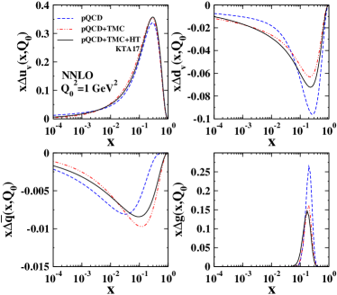
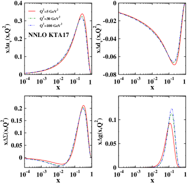
Figure 2 illustrates the evolution of KTA17 polarized parton distributions for a selection of $Q^{2}$ values of 5, 30, and 100 GeV². We observe that the evolution in all the distributions, except the gluon density, tends to flatten out the peak for increasing $Q^{2}$, While the gluon distribution increases in the large kinematic region of $x$.

Figure 2: (Color online) The KTA17 polarized parton distributions as a function of $x$ and for some selected value of Q² = 5, 30, 100 GeV².

IV.2 Polarized PDFs comparison

We present KTA17 PPDFs along with the corresponding uncertainty bounds as a function of $x$ at Q${}_{0}^{2}=$ 1 GeV² in Fig. 3. Various parameterizations of NNPDF Nocera:2014gqa KATAO Khorramian:2010qa , BB10 Blumlein:2010rn , DSSV09 deFlorian:2008mr , AAC09 Hirai:2008aj , AKS14 Arbabifar:2013tma , LSS06 Leader:2006xc and THK14 Monfared:2014nta at the NLO approximation, and TKAA16 Shahri:2016uzl at the NNLO approximation are illustrated for comparison. In the polarized PDF sets (NNPDF, LSS and DSSV) which include SIDIS and/or W boson production in polarized $pp$ collisions, $\Delta\bar{u}$ is different from $\Delta\bar{d}$, which are in turn different from $\frac{1}{2}(\Delta s+\Delta\bar{s})$. So we considered $\Delta\bar{q}=\frac{1}{2}(\Delta\bar{u}+\Delta\bar{d})$ in Fig. 3.

Figure 3: (Color online) KTA17 results for the polarized PDFs at Q${}_{0}^{2}=$ 1 GeV² as a function of $x$ in NNLO approximation plotted as a solid curve along with their $\Delta\chi^{2}=1$ uncertainty bands computed with the Hessian approach, as described in the text. We also show the result obtained in earlier global analyses of NNPDF(dashed-dotted-dotted) Nocera:2014gqa , KATAO (long dashed) Khorramian:2010qa , BB (dashed) Blumlein:2010rn , DSSV (dashed-dotted) deFlorian:2008mr , AAC09 (dashed-dashed-dotted) Hirai:2008aj in NLO approximation and TKAA16 (dotted) Shahri:2016uzl in the NNLO approximation.

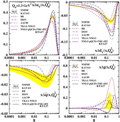
Our uncertainty estimation is based on the Hessian methods, for a tolerance of $\Delta\chi^{2}=1$. The $x\Delta u_{v}$ and $x\Delta d_{v}$ polarized PDFs are the best determined distributions from the inclusive polarized DIS data, with relatively smaller uncertainty bands for the $x\Delta u_{v}$ distribution. As one can see, our $x\Delta u_{v}$ is relatively compatible with other results while the $x\Delta d_{v}$, $x\Delta\bar{q}$ and $x\Delta g$ densities are treated differently. For the extrapolated regions, $x<10^{-3}$ and $x>0.8$, where the PPDFs are not directly constrained by the data, all valence distributions are treated the same.

The polarized gluon distribution is the most complicated case for PPDF uncertainties and parameterizations. Results for $x\Delta g$ from the various fits are usually quite spread. As illustrated in Fig. 3, the difficulty in constraining the polarized gluon distribution is clearly revealed through the spread of $x\Delta g$ from various global PPDF parametrizations. All the gluon distributions are positive at whole $x$ range, except for the KATAO, DSSV and NNPDF which indicate a sign change. The NNPF gluon density is treated differently in the small-$x$ region. The $x\Delta g$ distributions based on different group analyses tend to zero less quickly than the KTA17 result.

Large differences are visible over the whole $x$ range for the sea quark distribution. This distribution is actually not well constrained by the present polarized DIS data. It should be stressed again that, in both of our NNLO analyses, we used the inclusive DIS data to constrain polarized parton distributions. In contrast, in the fits of the LSS and DSSV collaborations,(SIDIS) data which are sensitive to the quark flavours are included. The quark-antiquark separation is achieved in NNPDF thanks to W boson production in polarized $pp$ collisions.

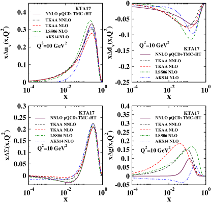
A detailed PPDF comparison is presented in Fig. 4, in which we plotted KTA17 together with those of TKAA16 (NLO and NNLO), AKS14 and LSS06 at Q${}^{2}=$ 10 GeV² as a function of $x$. Similar to previous comparisons, gluon density remains puzzling. The gluons from all PPDF sets are positive except for the AKS14 group which shows a sign change. The $x\Delta u_{v}$ and $x\Delta d_{v}$ polarized PDFs of the TKAA16 (NLO and NNLO), AKS14 and LSS06 are qualitatively similar, though for LSS06 $x\Delta u_{v}$ are typically larger at medium $x$.

Figure 4: (Color online) KTA17 results for the polarized PDFs at Q${}^{2}=$ 10 GeV² as a function of $x$ in NNLO approximation plotted as solid curves. Also shown are the recent results of TKAA16 (dotted) Shahri:2016uzl in both NLO and NNLO approximations, AKS14 Arbabifar:2013tma and LSS06 Leader:2006xc analysis.

IV.3 Polarized structure function comparison

Several efforts to study the nucleon structure have been developed, aiming to predict the polarized PDFs behavior at small and large $x$. In order to investigate the precision of the obtained polarized PDFs and also to test whether the DIS data favor or unfavor them, a detailed comparison of the extracted structure functions and the available polarized DIS data is required.

It should be stressed that much more numerous and more accurate data at both small and large $x$ are required to discriminate among different groups analyses. We will return to this subject in Sec. VI, considering an ongoing planned and proposed high-energy polarized collider.

In Figs. 5, 6, and 7, KTA17 theory predictions for the polarized structure functions of the proton $xg_{1}^{p}(x,Q^{2})$, neutron $xg_{1}^{n}(x,Q^{2})$ and deuteron $xg_{1}^{d}(x,Q^{2})$ are compared with the fixed-target DIS experimental data from E143, E154 and SMC. As we mentioned, KTA17 refers to the pQCD+TMC+HT scenario. The results from KATAO analysis in the NLO approximation Khorramian:2010qa and TKAA16 analysis in the NNLO approximation Shahri:2016uzl also shown. Our curves are presented for some selected values of $Q^{2}$ = 2, 3, 5, and 10 GeV² as a function of $x$. In general, we find good agreement with the experimental data over the entire range of $x$ and Q², and our results are in accord with other determinations.

Figure 5: (Color online) The spin-dependent proton structure functions as a function of $x$ and Q². KTA17 (solid curve) is compared with THK (dashed-dashed-dotted) Monfared:2014nta , KATAO (dashed) Khorramian:2010qa , TKAA16 (dashed dotted) Shahri:2016uzl .

Figure 6: (Color online) The spin-dependent neutron structure functions as a function of $x$ and Q². KTA17 (solid curve) is compared with THK (dashed-dashed-dotted) Monfared:2014nta , KATAO (dashed) Khorramian:2010qa , TKAA16 (dashed dotted) Shahri:2016uzl

Figure 7: (Color online) The spin-dependent deuteron structure functions as a function of $x$ and Q². KTA17 (solid curve) is compared with THK (dashed-dashed-dotted) Monfared:2014nta , KATAO (dashed) Khorramian:2010qa , TKAA16 (dashed dotted)  Shahri:2016uzl

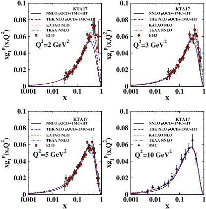
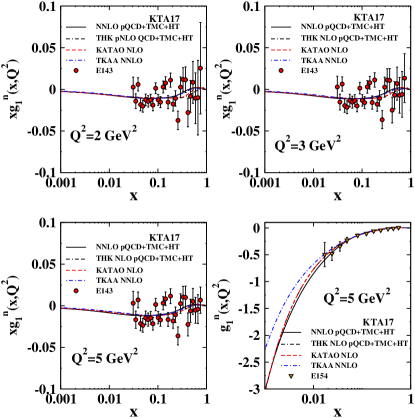
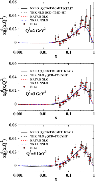
In Fig. 8, we check the consistency of KTA17 with the newly improved statistical precision data of COMPASS16 in the low-$x$ region.

Figure 8: (Color online) KTA17 prediction for the polarized proton structure function $g_{1}^{p}$ as a function of $x$ and for mean value of $Q^{2}=16$ GeV². Also shown are the most recent data from the COMPASS16 collaboration Adolph:2015saz . Note that the values of $Q^{2}$ for each data point are different.

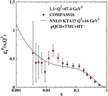
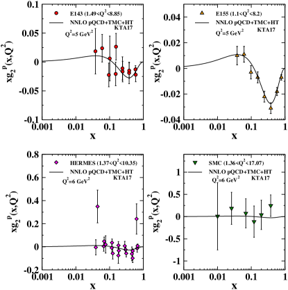
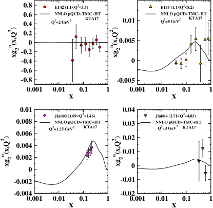
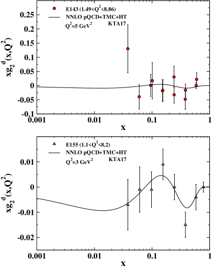
Further illustrations of the fit quality are presented in Figs. 9, 10 and 11 for the $xg_{2}^{i=p,n,d}(x,Q^{2})$ polarized structure functions obtained from Eq. (20). Generally the $g_{2}$ data have larger uncertainties compared with the $g_{1}$ data, reflecting the lack of knowledge in $g_{2}$ structure function. At the current level of accuracy, KTA17 is in agreement with data within their uncertainties, except for the E155 data for $xg_{2}^{d}(x,Q^{2})$. A precise quantitative extraction of the $xg_{2}(x,Q^{2})$ requires a large number of data with higher precision. Our results focus on the general characteristic of the $xg_{2}(x,Q^{2})$.

Figure 9: (Color online) KTA17 result for the proton structure functions $xg_{2}^{p}(x,Q^{2})$ as a function of $x$ and Q² compared to E143, E155, HERMES and SMC experimental data.

Figure 10: (Color online) KTA17 result for the neutron structure functions $xg_{2}^{n}(x,Q^{2})$ as a function of $x$ and Q² compared to E142, E155, JLAB03 and JLAB04 experimental data.

Figure 11: (Color online) KTA17 for the deuteron structure functions $xg_{2}^{d}(x,Q^{2})$ as a function of $x$ and Q² compared to E143 and E155 experimental data.

IV.4 Higher-twist contributions

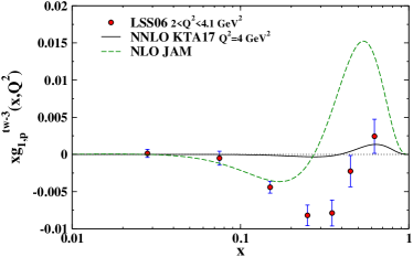
Figure 12 represents our $xg_{1}^{tw-3}(x,Q^{2})$ with those of LSS  Leader:2006xc and JAM13 Jimenez-Delgado:2013boa . LSS split the measured $x$ region into seven bins to determine the HT correction to $g_{1}$. They extracted the HT contribution in a model-independent way, while its scale dependence was ignored.The JAM group parametrized an analytical form for the twist-3 part of $g_{2}$ and calculated $g_{1}^{tw-3}$ by integral relation of Eq.( 19) in a global fit at NLO approximation.

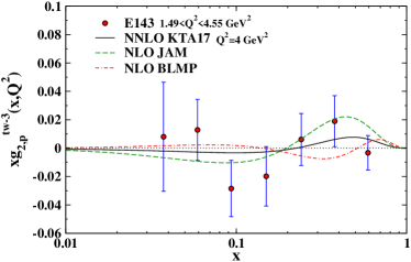
The twist-3 part of $g_{2}$ together with those of the JAM13 Jimenez-Delgado:2013boa and BLMP Braun:2011aw groups along with E143 experimental data Abe:1998wq are presented in Fig. 13. Keeping terms up to twist 3, E143 Collaboration at SLAC reported the twist 3 contribution to the proton spin structure function $xg_{2}^{p}$ with relatively large errors. However, within experimental precision the $g_{2}$ data are well described by the twist-2 contribution. The precision of the current data is not sufficient enough to distinguish model precision.

Figure 12: (Color online) The twist-3 contribution to $xg_{1}^{p}$ at $Q^{2}$=4 GeV² as a function of $x$ compared to the results of LSS Leader:2006xc and JAM13 Jimenez-Delgado:2013boa .

Figure 13: (Color online) The twist-3 contribution to $xg_{2}^{p}$ at $Q^{2}$ =4 GeV² as a function of $x$. KTA17 (solid curve) is compared with JAM13 Jimenez-Delgado:2013boa (dashed), BLMP Braun:2011aw (dashed dotted), and E143 experimental data Abe:1998wq .

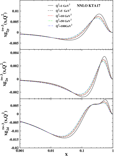
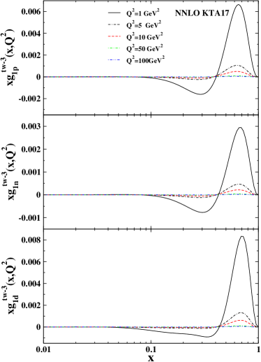
As illustrated in Fig. 14, the twist-3 part of $g_{2}$ has significant contribution even at large Q². In comparison with Fig. 15, we find that $xg_{\rm 1}^{\tau 3}$ vanishes rapidly at $Q^{2}>5$ GeV² while $xg_{\rm 2}^{\tau 3}$ remains nonzero even in the limit of Q${}^{2}\rightarrow\infty$.

Figure 14: (Color online) The twist-3 contribution of $xg_{2}$ for the proton, neutron, and deuteron as a function of $x$ and for different values of Q² according to the KTA17 NNLO analysis.

Figure 15: (Color online) The twist-3 contribution of $xg_{1}$ for the proton, neutron, and deuteron as a function of $x$ and for different values of Q² according to the KTA17 NNLO analysis.

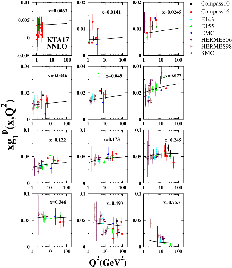
Finally, KTA17 QCD fit results on $xg_{1}$ are compared to experimental measurements in Fig. 16. These measurements come from the Compass10, Compass16, E143, E155, EMC, HERMES06, HERMES98 and SMC experiments. The curves are given vs $Q^{2}$ at several values of $x$ and are compared to the data. As can be seen, the theory predictions are in good agreement with the data.

Figure 16: (Color online) KTA17 theory predictions for the $xg_{1}(x,Q^{2})$ in comparison to DIS data from Compass10, Compass16, E143, E155, EMC, HERMES06, HERMES98 and SMC experiments.

V Sum Rules

Sum rules are powerful tools to investigate some fundamental properties of the nucleon structure, like the total momentum fraction carried by partons or the total contribution of parton spin to the spin of the nucleon. We explore how well the inclusion of TMCs and HT terms into NNLO polarized structure function analysis improves the precision of PPDF determination as well as QCD sum rules. In the following, the description of almost all important polarized sum rules together with available experimental data are briefly discussed.

V.1 Bjorken sum rule

The nonsinglet spin structure function is defined as

$$g_{1}^{\rm NS}(x,Q^{2}) = g_{1}^{p}(x,Q^{2})-g_{1}^{n}(x,Q^{2})\,.$$ (26)

The polarized Bjorken sum rule expresses the integral over the spin distributions of quarks inside of the nucleon in terms of its axial charge times a coefficient function Bjorken:1969mm as

$$\Gamma_{1}^{\rm NS}(Q^{2}) = \Gamma_{1}^{p}(Q^{2})-\Gamma_{1}^{n}(Q^{2})$$

$$= \int_{0}^{1}[g_{1}^{p}(x,Q^{2})-g_{1}^{{n}}(x,Q^{2})]dx$$

$$= \frac{1}{6}\leavevmode\nobreak\ |g_{A}|\leavevmode\nobreak\ C_{Bj}[\alpha_{s}(Q^{2})]+\text{HT corrections}\,.$$

Here, $g_{A}$ is the nucleon axial charge as measured in neutron $\beta$ decay. The coefficient function $C_{Bj}[\alpha_{s}(Q^{2})]$ is calculated in four-loop pQCD corrections in the massless Baikov:2010je and very recently massive cases Blumlein:2016xcy . Bjorken sum rule potentially provides a very precise handle on the strong coupling constant. The value of $\alpha_{s}$ can be extracted via $C_{Bj}[\alpha_{s}(Q^{2})]$ expression from experimental data. $\alpha_{s}$ is also available form accurate methods, such as the $\tau$ lepton and the $Z$ boson into hadrons width decay. Comparison of these values offers an important test of QCD consistency. As previously reported in Ref. Altarelli:1998nb , determination of $\alpha_{s}$ from the Bjorken sum rule suffers from small-$x$ extrapolation ambiguities.

Our results for the Bjorken sum rule are compared with experimental measurements E143 Abe:1998wq , SMC SMCpg2 , HERMES06 HERMpd and COMPASS16 Adolph:2015saz in Table 4.

Table 4: Comparison of the result of the Bjorken sum rule for $\Gamma_{1}^{NS}$ with world data from E143 Abe:1998wq , SMC SMCpg2 , HERMES06 HERMpd and COMPASS16 Adolph:2015saz . Only HERMES06 HERMpd results are not extrapolated in full $x$ range (measured in region $0.021\leq x\leq 0.9$).

	E143 Abe:1998wq	SMC SMCpg2	HERMES06 HERMpd	COMPASS16 Adolph:2015saz	KTA17
	$Q^{2}=5$ GeV2	$Q^{2}=5$ GeV2	$Q^{2}=5$ GeV2	$Q^{2}=3$ GeV2	$Q^{2}=5$ GeV2
$\Gamma^{\rm NS}_{1}$	$0.164\pm 0.021$	$0.181\pm 0.035$	$0.148\pm 0.017$	$0.181\pm 0.008$	$0.173\pm 0.003$

V.2 Proton helicity sum rule

The extrapolation of the proton spin among its constituents is a compelling question still driving the field of nuclear physics Leader:2016sli . In order to get an accurate picture of the quark and gluon helicity density a precise extraction of PPDFs entering the proton’s momentum sum rule is required. In a general approach, the spin of the nucleon can be carried by its constituents as

$$\frac{1}{2}=\frac{1}{2}\Delta\Sigma(Q^{2})+\Delta{\mathrm{G}}(Q^{2})+{\mathrm{L}}(Q^{2}).$$ (28)

Here, $\Delta{\rm G(Q^{2})}=\int_{0}^{1}dx\leavevmode\nobreak\ \Delta g(x,Q^{2})$ has the interpretation of the gluon spin contribution, and $\Delta\Sigma(Q^{2})=\sum_{i}\int_{0}^{1}dx\leavevmode\nobreak\ (\Delta q(x,Q^{2})+\Delta\bar{q}(x,Q^{2}))$ denotes the flavor singlet spin contribution. ${\mathrm{L}}(Q^{2})$ is the total contribution from the quark and gluon orbital angular momentum. Finding a way to measure them is a real challenge beyond the scope of this paper. Each individual term in Eq. (28) is a function of $Q^{2}$n but the sum is not. The values of the singlet-quark and gluon first moment at the scale of Q²=10 GeV² are listed in Table 5. Results are compared to those from the NNPDFpol1.0 Ball:2013lla , NNPDFpol1.1 Nocera:2012hx and DSSV08 deFlorian:2008mr at both the truncated and full $x$ regions. In Table 6, KTA17 results are presented and compared at Q²=4 GeV² with the DSSV08 deFlorian:2008mr , BB10 Blumlein:2010rn , LSS10 Leader:2010rb and NNPDFpol1.0 Ball:2013lla results.

Coming now to a comparison of results, we see that for the $\Delta\Sigma$, KTA17 results are consistent within uncertainties with that of other groups. This is mainly because the first moment of polarized densities is fixed by semileptonic decays. Turning to the gluon, very different values are reported. The large uncertainty prevents reaching a firm conclusion about the full first moment of the gluon.

Table 5: Results for the full and truncated first moments of the polarized singlet-quark $\Delta\Sigma(Q^{2})=\sum_{i}\int_{0}^{1}dx[\Delta q_{i}(x)+\Delta\bar{q}_{i}(x)]$ and gluon distributions at the scale Q²=10 GeV² in the $\overline{{\rm MS}}$ scheme. Also shown are the recent polarized global analyses of NNPDFpol1.0 Ball:2013lla , NNPDFpol1.1 Nocera:2012hx and DSSV08 deFlorian:2008mr .

	DSSV08 deFlorian:2008mr	NNPDFpol1.0 Ball:2013lla	NNPDFpol1.1 Nocera:2012hx	KTA17
Full $x$ region $[0,1]$
$\Delta\Sigma{\rm(Q^{2})}$	$0.242$	$+0.16\pm 0.30$	$+0.18\pm 0.21$	$0.210\pm 0.045$
$\Delta{\rm G(Q^{2})}$	$-0.084$	$-0.95\pm 3.87$	$0.03\pm 3.24$	$0.138\pm 0.058$
Truncated $x$ region [$10^{-3},1$]
$\Delta\Sigma{\rm(Q^{2})}$	$0.366\pm 0.017$	$+0.23\pm 0.15$	$+0.25\pm 0.10$	$0.234\pm 0.044$
$\Delta{\rm G(Q^{2})}$	$0.013\pm 0.182$	$-0.06\pm 1.12$	$0.49\pm 0.75$	$0.138\pm 0.058$

Table 6: Same as Table 5, but only for the full first moments of the polarized singlet-quark and gluon distributions at the scale Q² =4 GeV² in the $\overline{{\rm MS}}$ scheme. Those of DSSV08 deFlorian:2008mr , BB10 Blumlein:2010rn , LSS10 Leader:2010rb and NNPDFpol1.0 Ball:2013lla are presented for comparison.

	DSSV08 deFlorian:2008mr	BB10 Blumlein:2010rn	LSS10 Leader:2010rb	NNPDFpol1.0 Ball:2013lla	KTA17
$\Delta\Sigma{\rm(Q^{2})}$	$0.245$	$0.193\pm 0.075$	$0.207\pm 0.034$	$0.18\pm 0.20$	$0.232\pm 0.044$
$\Delta{\rm G(Q^{2})}$	$-0.096$	$0.462\pm 0.430$	$0.316\pm 0.190$	$-0.9\pm 4.2$	$0.128\pm 0.053$

Let us finally discus the proton spin sum rule based on the extracted values presented in Table 6. The total orbital angular momentum to the total spin of the proton is

$${\mathrm{L}}(Q^{2}=4\leavevmode\nobreak\ \rm GeV^{2})=0.256\pm 0.069\,.$$ (29)

The gluon uncertainty is clearly dominant. Due to large uncertainty originating mainly from the gluons, we cannot yet come to a definite conclusion about the contribution of the total orbital angular momentum to the spin of the proton. Improving the current level of experimental accuracy is required for the precise determination of each individual contribution.

V.3 twist 3 reduced matrix element $d_{2}$

Under the OPE, one can study the effect of quark-gluon correlations via the moments of $g_{1}$ and $g_{2}$

$$d_{2}(Q^{2}) = 3\int_{0}^{1}x^{2}\bar{g_{2}}(x,Q^{2})\leavevmode\nobreak\ dx$$ (30)

$$= \int_{0}^{1}x^{2}[3g_{2}(x,Q^{2})+2g_{1}(x,Q^{2})]\leavevmode\nobreak\ dx,$$

as follows from the relation $\bar{g}_{2}=g_{2}-g_{2}^{WW}$. Thus, the twist-3 reduced matrix element of spin-dependent operators in the nucleon measures the deviation of $g_{2}$ from $g_{2}^{\tau 2}$ [See Eq. (14)]. The function of $d_{2}(Q^{2})$ is especially sensitive to the large-$x$ behavior of $\bar{g_{2}}$ (due to the $x^{2}$ weighting factor). Extraction of $d_{2}$ is particularly interesting as it will provide insight into the size of the multiparton correlation terms.

Our results together with the other theoretical and experimental values are presented in Table 7. This notably nonzero value for $d_{2}$ implies the significance of considering higher-twist terms in QCD analyses. The most reliable determination of the the higher-twist moments $d_{2}$ was performed in JAM15 Sato:2016tuz . Since they are the only group that implemented TMCs for the $\tau 3$ part.

In the near future, the expected data from 12 GeV Jefferson Lab experiments JLAB-12 may enable the $d_{2}$ moments to be determined more precisely in the DIS region at higher $Q^{2}$ values. QCD analysis of this new generation of bounded uncertainty data requires including TMCs in all higher-twist terms.

Table 7: $d_{2}$ moments of the proton, neutron and deuteron polarized structure functions from the SLAC E155x Kuhn:2008sy , E01-012 Solvignon:2013yun , E06-014 Flay:2016wie , Lattice QCD Gockeler:2005vw , CM bag model Song:1996ea , JAM15 Sato:2016tuz , and JAM13 Jimenez-Delgado:2013boa compared with KTA17 results.

	Ref.	$Q^{2}$ [GeV2]	$10^{2}d^{p}_{2}$	$10^{5}d^{n}_{2}$	$10^{3}d^{d}_{2}$
KTA17		$5$	$0.66\pm 0.01$	$193.81\pm 6.42$	$6.97\pm 0.11$
E06-014	Flay:2016wie	3.21		$-421.0\pm 79.0\pm 82.0\pm 8.0$	-
E06-014	Flay:2016wie	4.32		$-35.0\pm 83.0\pm 69.0\pm 7.0$	-
E01-012	Solvignon:2013yun	3	-	$-117\pm 88\pm 138$	-
E155x	E155pdg2	$5$	$0.32\pm 0.17$	$790\pm 480$	-
E143	Abe:1998wq	$5$	$0.58\pm 0.50$	$500\pm 2100$	$5.1\pm 9.2$
Lattice QCD	Gockeler:2005vw	5	0.4(5)	-100(-300)	-
CM bag model	Song:1996ea	$5$	$1.74$	$-253$	$6.79$
JAM15	Sato:2016tuz	$1$	$0.5\pm 0.2$	$-100\pm 100$	-
JAM13	Jimenez-Delgado:2013boa	$5$	$1.1\pm 0.2$	$200\pm 300$	-

V.4 Burkhardt-Cottingham (BC) sum rule

The first moment of $g_{2}$ is predicted to yield zero by Burkhardt and Cottingham (BC) from virtual Compton scattering dispersion relations in all Q² Burkhardt:1970ti

$$\Gamma_{2}=\int_{0}^{1}dx\,g_{2}(x,Q^{2})=0\leavevmode\nobreak\ .$$ (31)

It appears to be a trivial consequence of the WW relation for $g_{2}^{\tau 2}$. The BC sum rule is also satisfied for the target mass corrected structure functions. Therefore a violation of the BC sum rule would imply the presence of HT contributions hermes2012g2 . Our $\Gamma_{2}$ results together with data from the E143 Abe:1998wq , E155 E155pdg2 , HERMES2012 hermes2012g2 , RSS Slifer:2008xu , and E01012 Solvignon:2013yun groups for the proton, deuteron and neutron are presented in Table 8. Any conclusion depends on the low-$x$ behavior of $g_{2}$ which has not yet been precisely measured.

Table 8: Comparison of the result of the BC sum rule for $\Gamma_{2}^{p}$, $\Gamma_{2}^{d}$ and $\Gamma_{2}^{n}$ with world data from E143 Abe:1998wq , E155 E155pdg2 , HERMES2012 hermes2012g2 , RSS Slifer:2008xu , and E01012 Solvignon:2013yun .

	E143 Abe:1998wq	E155 E155pdg2	HERMES2012 hermes2012g2	RSS Slifer:2008xu	E01012 Solvignon:2013yun	KTA17
	$0.03\leq x\leq 1$	$0.02\leq x\leq 0.8$	$0.023\leq x\leq 0.9$	$0.316<x<0.823$	$0\leq x\leq 1$	$0.03\leq x\leq 1$
	$Q^{2}=5$ GeV2	$Q^{2}=5$ GeV2	$Q^{2}=5$ GeV2	$Q^{2}=1.28$ GeV2	$Q^{2}=3$ GeV2	$Q^{2}=5$ GeV2
$\Gamma_{2}^{p}$	$-0.014\pm 0.028$	$-0.044\pm 0.008$	$0.006\pm 0.029$	$-0.0006\pm 0.0022$	…	$-0.0171\pm 0.0004$
$\Gamma_{2}^{d}$	$-0.034\pm 0.082$	$-0.008\pm 0.012$	-	$-0.0090\pm 0.0026$	…	$-0.0051\pm 0.0008$
$\Gamma_{2}^{n}$	-	-	-	$-0.0092\pm 0.0035$	$0.00015\pm 0.00113$	$\leavevmode\nobreak\ 0.0080\pm 0.0013$

V.5 Efremov-Leader-Teryaev sum rule

The Efremov-Leader-Teryaev (ELT) sum rule Efremov:1996hd integrates the valence part of $g_{1}$ and $g_{2}$ over $x$. Considering that the sea quarks are the same in protons and neutrons, the ELT sum rule can be derived similar to the Bjorken sum rule as

$$\int_{0}^{1}dx\leavevmode\nobreak\ x[g_{1}^{V}(x)+2g_{2}^{V}(x)]=$$

$$\int_{0}^{1}dx\leavevmode\nobreak\ x[g_{1}^{p}(x)-g_{1}^{n}(x)+2(g_{2}^{p}(x)-g_{2}^{n}(x))]=0.$$ (32)

This sum rule receives quark mass corrections and is only valid in the case of massless quarks Blumlein:1996vs . It is preserved under the presence of target mass corrections Blumlein:1998nv . Combining the data of E143 Abe:1998wq and E155 E155pdg2 leads to $-0.011\pm 0.008$ at Q²=5 GeV². We extracted the value of $0.0063\pm 0.0003$ at the same Q².

VI Polarized PDFs in the high-precision era of collider physics

Several determinations of polarized PDFs of the proton are presently available up to NLO  deFlorian:2009vb ; Hirai:2008aj ; Blumlein:2010rn ; Leader:2010rb ; Nocera:2014gqa ; Jimenez-Delgado:2013boa ; Jimenez-Delgado:2014xza ; Sato:2016tuz ; Arbabifar:2013tma ; Monfared:2014nta and also for the NNLO approximation Shahri:2016uzl . They mostly differ in the included polarized data sets, the procedure applied to determine PPDFs from these data sets and the method used to extract corresponding uncertainties. Most of the analyses focused on the Lagrange multiplier or the Hessian approaches to estimate the uncertainty, while the NNPDF collaboration has developed a Monte Carlo methodology to control uncertainties. Available analyses use experimental information from neutral-current DIS and SIDIS to constrain the total quark combinations and individual quark and antiquark flavors, respectively. The gluon distribution would be constrained rather weakly by both DIS and SIDIS data, because of the small $Q^{2}$ range covered.

In addition to the DIS and SIDIS fixed-target data, a remarkable amount of data from longitudinally polarized proton-proton collisions at the RHIC has become available recently Aschenauer:2016our ; Akiba:2015jwa . The RHIC data can be expected to further constrain the gluon helicity distribution especially at the small momentum fractions, down to $x\sim 0.01$ Aschenauer:2013woa ; Aschenauer:2015eha ; Ball:2013tyh ; Adare:2015ozj . The double-helicity asymmetries for jet and $\pi^{0}$ production are directly sensitive to the gluon helicity distribution over a small range of $x$, because of the dominance of gluon-gluon and quark-gluon initiated subprocesses in the kinematic range accessed by PHENIX at the RHIC Adare:2014wht . In recent helicity PDF fits deFlorian:2008mr ; deFlorian:2009vb ; Nocera:2014gqa ; deFlorian:2014yva , the RHIC measurements on the double-longitudinal spin asymmetry in the production of hadrons Adare:2008aa ; Adare:2008qb and inclusive jet production in $pp$ collisions Abelev:2007vt , as well as single-longitudinal spin asymmetry measurements in the production of $W^{\pm}$ bosons Aggarwal:2010vc ; Adare:2010xa ; Nocera:2016xhb , have already been used. These data can increase sensitivity to the sign information of gluon density in present and future pQCD helicity PDF fits. In addition to the mentioned data, inclusion of the Hall-A and CLASS measurements at JLAB leads to a reduction in the PDF errors for the polarized valence and sea quarks densities as well as the gluon polarization uncertainty at $x\geqslant 0.1$ Sato:2016tuz .

The COMPASS Collaboration at CERN performed new measurements of the longitudinal double-spin asymmetry and the longitudinal spin structure function of the proton Adolph:2015saz as well as deuteron Adolph:2016myg . COMPASS measurements provide the lowest accessible values for $x$ and the largest $Q^{2}$ values for any given $x$. Consequently, it leads to a better determination of sea quarks and gluon helicity distribution including the corresponding uncertainties. These data improve the statistical precision of $g^{p}_{1}(x)$ by about a factor of 2 in the region $x\leqslant 0.02$.

Despite the discussed achievements, the QCD analysis of polarized data suffers from both limited kinematic coverage and insufficient precision of the available inclusive data. Consequently our understanding of the nucleon spin structure is still far from complete. The most up-to-date 200 GeV data from the COMPASS16 experiment do not change much the general trend of the polarized PDFs but a reduction of the uncertainties on almost all parton species was observed.

Finally, it should be stressed that a future polarized electron-ion collider (EIC) would allow for a major breakthrough toward the understanding of the proton spin. The EIC is expected to open up the kinematic domain to significantly lower values of $x$ ($x\approx 10^{-4}$) in center-of-mass energy to $\sim 104$ GeV², reducing significantly the uncertainty on the contributions from the unmeasured small-$x$ region. The EIC will likely be the only facility to study the spin structure of the proton with the highest precision Chu:2016wsq ; Accardi:2012qut ; Nocera:2016xhb ; Chudakov:2016ytj ; Montgomery:2016uws ; Cosyn:2016oiq ; Cosyn:2014zfa ; Guzey:2014jva ; Hoecker:2016vvy .

VII Summary and conclusions

The main goal of the present KTA17 analysis is to determine the nucleon spin structure functions $g_{1}(x,Q^{2})$ and $g_{2}(x,Q^{2})$ and their moments which are essential in testing QCD sum rules. We have enriched our recent NNLO formalism Shahri:2016uzl by TMCs and HT terms and extended it to include more experimental observables. These corrections play a significant role in the large-$x$ region at low $Q^{2}$. We achieved an excellent description of the fitted data and provided unified and consistent PPDFs. Our helicity distributions have compared reasonably well with other extractions, within the known very large uncertainties arising from the lack of constraining data. We also studied the TMCs and HT effects on several sum rules at the NNLO approximation, since they are relevant in the region of low $Q^{2}$. The Bjorken sum rule is related to polarized $g_{1}$ structure functions. We also present our results for the reduced matrix element $d_{2}$ in the NNLO approximation. More accurate data are required to scrutinize the BC and ELT sum rules.

The future polarized EIC will make a huge impact on our knowledge of spin physics. The decreased uncertainties would absolutely solve the question of how spin and the orbital angular momentum of partons contribute to the overall proton spin. Concluding, in the light of upcoming development in experimental projects, phenomenological efforts to increase our knowledge of the nucleon structure functions and their moments are particularly important.

Appendix A FORTRAN package of KTA17 NNLO polarized PDFs

A FORTRAN package containing KTA17 NNLO spin-dependent PDFs as well as the polarized structure functions $x\,g_{1}^{i=p,n,d}(x,Q^{2})$ for the proton, neutron and deuteron can be obtained via Email from the authors upon request. This package also includes an example program to illustrate the use of the routines.

Appendix B NNLO splitting function

In this section, for completeness, we present the NNLO Mellin-N space splitting function used for the evolution of longitudinally polarized parton densities based on our analysis. Their $x$-space forms are available in Ref. Moch:2014sna . FORTRAN files of our analytical results can be obtained from the authors upon request.

These function can be written in terms of the harmonic sums as Vermaseren:1998uu ; Blumlein:1998if ,

$$s_{1} = \gamma_{E}+\psi(n+1)\,,$$

$$s_{2} = \zeta(2)-\psi^{\prime}(n+1)\,,$$

$$s_{3} = \zeta(3)+0.5\,\psi^{\prime\prime}(n+1)\,,$$

$$s_{4} = \zeta(4)-1/6\,\psi^{\prime\prime\prime}(n+1),$$

where $\gamma_{E}=0.577216$ is the Euler constant, $\psi(n)=d\ln\Gamma(n)/dn$ is the digamma function and $\zeta(2)=\pi^{2}/6$, $\zeta(3)=1.20206$ and $\zeta(4)=1.08232$.

The analytical expressions for the polarized NNLO quark-quark splitting function are given by

$$\Delta p_{qq}^{(2)}=1295.47+\frac{928}{27n^{5}}-\frac{640}{3n^{4}}+\frac{798.4}{n^{3}}-\frac{1465.2}{n^{2}}+\frac{1860.2}{n}-\frac{3505}{1+n}+\frac{297}{2+n}-\frac{433.2}{3+n}+$$

$$1174.898\left(\frac{1}{n}-s_{1}\right)-\frac{714.1s_{1}}{n}+684\left(\frac{s_{1}}{n^{2}}+\frac{-\zeta(2)+s_{2}}{n}\right)+$$

$$f\left(-173.933+\frac{512}{27n^{4}}-\frac{2144}{27n^{3}}+\frac{172.69}{n^{2}}-\frac{216.62}{n}+\frac{6.816}{(1+n)^{4}}+\frac{406.5}{1+n}+\frac{77.89}{2+n}+\right.$$

$$\left.\frac{34.76}{3+n}-183.187\left(\frac{1}{n}-s_{1}\right)+\frac{5120s_{1}}{81n}-65.43\left(\frac{s_{1}}{n^{2}}+\frac{-\zeta(2)+s_{2}}{n}\right)\right)+$$

$$\frac{32}{3}f^{2}\left(-\frac{17}{72}+\frac{3-2n-12n^{2}+2n^{3}+12n^{4}}{27n^{3}(1+n)^{3}}+\frac{2s_{1}}{27}+\frac{10s_{2}}{27}-\frac{2s_{3}}{9}\right)+$$

$$502.4\left(-\frac{s_{1}}{n^{3}}+\frac{\zeta(2)-s_{2}}{n^{2}}-\frac{-\zeta(3)+s_{3}}{n}\right)\,.$$

For the gluon-quark splitting functions we have

$$\Delta p_{qg}^{(2)}=f\left(-\frac{1208}{n^{5}}+\frac{2313.84}{n^{4}}-\frac{1789.6}{n^{3}}+\frac{1461.2}{n^{2}}-\frac{2972.4}{n}+\frac{439.8}{(1+n)^{4}}+\frac{2290.6}{(1+n)^{3}}+\frac{4672}{1+n}-\right.$$

$$\frac{1221.6}{2+n}-\frac{18}{3+n}-\frac{278.32s_{1}}{n}-\frac{90.26\left(s_{1}{}^{2}+s_{2}\right)}{n}+825.4\left(\frac{s_{1}}{n^{2}}+\frac{-\zeta(2)+s_{2}}{n}\right)+$$

$$f\left(\frac{128}{3n^{5}}-\frac{184.434}{n^{4}}+\frac{393.92}{n^{3}}-\frac{526.3}{n^{2}}+\frac{499.65}{n}-\frac{61.116}{(1+n)^{4}}+\frac{358.2}{(1+n)^{3}}-\right.$$

$$\frac{432.18}{1+n}-\frac{141.63}{2+n}-\frac{11.34}{3+n}+\frac{6.256s_{1}}{n}+\frac{7.32\left(s_{1}{}^{2}+s_{2}\right)}{n}-47.3\left(\frac{s_{1}}{n^{2}}+\frac{-\zeta(2)+s_{2}}{n}\right)+$$

$$\left.\frac{0.7374\left(-s_{1}{}^{3}-3s_{1}s_{2}-2s_{3}\right)}{n}\right)-\frac{5.3\left(-s_{1}{}^{3}-3s_{1}s_{2}-2s_{3}\right)}{n}+$$

$$\left.\frac{3.784\left(s_{1}{}^{4}+6s_{1}{}^{2}s_{2}+3s_{2}{}^{2}+8s_{1}s_{3}+6s_{4}\right)}{n}\right)\,,$$

$$\Delta p_{gq}^{(2)}=\frac{92096}{27n^{5}}-\frac{5328.018}{n^{4}}+\frac{4280}{n^{3}}-\frac{4046.6}{n^{2}}+\frac{6159}{n}-\frac{1050.6}{(1+n)^{4}}-\frac{1701.4}{(1+n)^{3}}-\frac{3825.9}{1+n}+$$

$$\frac{1942}{2+n}-\frac{742.1}{3+n}-\frac{1843.7s_{1}}{n}+\frac{451.55\left(s_{1}{}^{2}+s_{2}\right)}{n}-1424.8\left(\frac{s_{1}}{n^{2}}+\frac{-\zeta(2)+s_{2}}{n}\right)+$$

$$f\left(-\frac{1024}{9n^{5}}+\frac{236.3232}{n^{4}}-\frac{404.92}{n^{3}}+\frac{308.98}{n^{2}}-\frac{301.07}{n}+\frac{180.138}{(1+n)^{4}}-\frac{253.06}{(1+n)^{3}}-\right.$$

$$\frac{296}{1+n}+\frac{406.13}{2+n}-\frac{101.62}{3+n}+\frac{171.78s_{1}}{n}-\frac{47.86\left(s_{1}{}^{2}+s_{2}\right)}{n}-16.18\left(\frac{s_{1}}{n^{2}}+\frac{-\zeta(2)+s_{2}}{n}\right)+$$

$$\frac{16}{27}f\left(-\frac{12}{n}+\frac{10}{1+n}+\frac{2}{1+n}\left(-\frac{1}{1+n}-s_{1}\right)-\frac{8\text{ss}_{1}}{n}+\frac{6\left(s_{1}{}^{2}+s_{2}\right)}{n}-\right.$$

$$\left.\left.\frac{3}{1+n}\left(\frac{1}{(1+n)^{2}}+\left(\frac{1}{1+n}+s_{1}\right){}^{2}+s_{2}\right)\right)-\frac{4.963\left(-s_{1}{}^{3}-3s_{1}s_{2}-2s_{3}\right)}{n}\right)+$$

$$\frac{59.3\left(-s_{1}{}^{3}-3s_{1}s_{2}-2s_{3}\right)}{n}+\frac{5.143\left(s_{1}{}^{4}+6s_{1}{}^{2}s_{2}+3s_{2}{}^{2}+8s_{1}s_{3}+6s_{4}\right)}{n}\,.$$

Finally, the polarized third-order gluon-gluon splitting function reads:

$$\Delta p_{gg}^{(2)}=4427.762+\frac{12096}{n^{5}}-\frac{22665}{n^{4}}+\frac{21804}{n^{3}}-\frac{23091}{n^{2}}+\frac{30988}{n}-\frac{7002}{(1+n)^{4}}-\frac{1726}{(1+n)^{3}}-$$

$$\frac{39925}{1+n}+\frac{13447}{2+n}-\frac{4576}{3+n}+2643.521\left(\frac{1}{n}-s_{1}\right)-\frac{3801s_{1}}{n}-$$

$$13247\left(-\frac{1}{1+n}\left(-\frac{1}{1+n}-s_{1}\right)-\frac{s_{1}}{n}\right)-12292\left(\frac{s_{1}}{n^{2}}+\frac{-\zeta(2)+s_{2}}{n}\right)+$$

$$f\left(-528.536-\frac{6128}{9n^{5}}+\frac{2146.788}{n^{4}}-\frac{3754.4}{n^{3}}+\frac{3524}{n^{2}}-\frac{1173.5}{n}-\frac{786}{(1+n)^{4}}+\right.$$

$$\frac{1226.2}{(1+n)^{3}}+\frac{2648.6}{1+n}-\frac{2160.8}{2+n}+\frac{1251.7}{3+n}-412.172\left(\frac{1}{n}-s_{1}\right)+\frac{295.7s_{1}}{n}-$$

$$6746\left(-\frac{1}{1+n}\left(-\frac{1}{1+n}-s_{1}\right)-\frac{s_{1}}{n}\right)-7932\left(\frac{s_{1}}{n^{2}}+\frac{-\zeta(2)+s_{2}}{n}\right)+$$

$$f\left(6.4607\,+\frac{7.0854}{n^{4}}-\frac{13.358}{n^{3}}+\frac{13.29}{n^{2}}-\frac{16.606}{n}+\frac{31.528}{(1+n)^{3}}+\frac{32.905}{1+n}-\right.$$

$$\left.\left.\frac{18.3}{2+n}+\frac{2.637}{3+n}-\frac{16}{9}\left(\frac{1}{n}-s_{1}\right)+\frac{0.21s_{1}}{n}-16.944\left(\frac{s_{1}}{n^{2}}+\frac{-\zeta(2)+s_{2}}{n}\right)\right)\right)\,.$$

For completeness, we also include the polarized NNLO pure singlet contribution,

$$\Delta p_{ps}^{(2)}=f\left(-\frac{344}{27}\left(\frac{24}{n^{5}}-\frac{24}{(1+n)^{5}}\right)-90.9198\left(-\frac{6}{n^{4}}+\frac{6}{(1+n)^{4}}\right)-368.6\left(\frac{2}{n^{3}}-\frac{2}{(1+n)^{3}}\right)-\right.$$

$$739\left(-\frac{1}{n^{2}}+\frac{1}{(1+n)^{2}}\right)-1362.6\left(\frac{1}{n}-\frac{1}{1+n}\right)-81.5\left(-\frac{6}{(1+n)^{4}}+\frac{6}{(2+n)^{4}}\right)+$$

$$349.9\left(\frac{2}{(1+n)^{3}}-\frac{2}{(2+n)^{3}}\right)+1617.4\left(\frac{1}{1+n}-\frac{1}{2+n}\right)-674.8\left(\frac{1}{2+n}-\frac{1}{3+n}\right)+$$

$$167.41\left(\frac{1}{3+n}-\frac{1}{4+n}\right)-204.76\left(-\frac{-\frac{1}{1+n}-s_{1}}{1+n}-\frac{s_{1}}{n}\right)+$$

$$232.57\left(\frac{s_{1}}{n^{2}}-\frac{\frac{1}{1+n}+s_{1}}{(1+n)^{2}}+\frac{-\zeta(2)+s_{2}}{n}-\frac{\frac{1}{(1+n)^{2}}-\zeta(2)+s_{2}}{1+n}\right)-$$

$$12.61\left(\frac{s_{1}{}^{2}+s_{2}}{n}-\frac{\frac{1}{(1+n)^{2}}+\left(\frac{1}{1+n}+s_{1}\right){}^{2}+s_{2}}{1+n}\right)+$$

$$f\left(1.1741\left(-\frac{6}{n^{4}}+\frac{6}{(1+n)^{4}}\right)+13.287\left(\frac{2}{n^{3}}-\frac{2}{(1+n)^{3}}\right)+45.482\left(-\frac{1}{n^{2}}+\frac{1}{(1+n)^{2}}\right)+\right.$$

$$49.13\left(\frac{1}{n}-\frac{1}{1+n}\right)-0.8253\left(-\frac{6}{(1+n)^{4}}+\frac{6}{(2+n)^{4}}\right)+$$

$$10.657\left(\frac{2}{(1+n)^{3}}-\frac{2}{(2+n)^{3}}\right)-30.77\left(\frac{1}{1+n}-\frac{1}{2+n}\right)-4.307\left(\frac{1}{2+n}-\frac{1}{3+n}\right)-$$

$$0.5094\left(\frac{1}{3+n}-\frac{1}{4+n}\right)+9.517\left(-\frac{1}{1+n}\left(-\frac{1}{1+n}-s_{1}\right)-\frac{s_{1}}{n}\right)+$$

$$\left.1.7805\left(\frac{s_{1}{}^{2}+s_{2}}{n}-\frac{1}{1+n}\left(\frac{1}{(1+n)^{2}}+\left(\frac{1}{1+n}+s_{1}\right){}^{2}+s_{2}\right)\right)\right)-$$

$$6.541\left(\frac{-s_{1}{}^{3}-3s_{1}s_{2}-2s_{3}}{n}-\right.$$

$$\left.\left.\frac{1}{1+n}\left(-\left(\frac{1}{1+n}+s_{1}\right){}^{3}-3\left(\frac{1}{1+n}+s_{1}\right)\left(\frac{1}{(1+n)^{2}}+s_{2}\right)-2\left(\frac{1}{(1+n)^{3}}+s_{3}\right)\right)\right)\right).$$

References

- (1) C. A. Aidala, S. D. Bass, D. Hasch and G. K. Mallot, Rev. Mod. Phys. 85, 655 (2013).
- (2) R. D. Ball, E. R. Nocera and J. Rojo, “The asymptotic behaviour of parton distributions at small and large ,” Eur. Phys. J. C. 76, 383 (2016).
- (3) D. de Florian, R. Sassot, M. Stratmann and W. Vogelsang, “Extraction of Spin-Dependent Parton Densities and Their Uncertainties,” Phys. Rev. D 80, 034030 (2009).
- (4) M. Hirai et al. [Asymmetry Analysis Collaboration], “Determination of gluon polarization from deep inelastic scattering and collider data,” Nucl. Phys. B 813, 106 (2009).
- (5) J. Blumlein and H. Bottcher, “QCD Analysis of Polarized Deep Inelastic Scattering Data,” Nucl. Phys. B 841, 205 (2010).
- (6) E. Leader, A. V. Sidorov and D. B. Stamenov, “Determination of Polarized PDFs from a QCD Analysis of Inclusive and Semi-inclusive Deep Inelastic Scattering Data,” Phys. Rev. D 82, 114018 (2010).
- (7) E. R. Nocera et al. [NNPDF Collaboration], “A first unbiased global determination of polarized PDFs and their uncertainties,” Nucl. Phys. B 887, 276 (2014).
- (8) P. Jimenez-Delgado, A. Accardi and W. Melnitchouk, “Impact of hadronic and nuclear corrections on global analysis of spin-dependent parton distributions,” Phys. Rev. D 89, no. 3, 034025 (2014).
- (9) P. Jimenez-Delgado et al. [Jefferson Lab Angular Momentum (JAM) Collaboration], “Constraints on spin-dependent parton distributions at large from global QCD analysis,” Phys. Lett. B 738, 263 (2014).
- (10) N. Sato et al. [Jefferson Lab Angular Momentum Collaboration], “Iterative Monte Carlo analysis of spin-dependent parton distributions,” Phys. Rev. D 93, no. 7, 074005 (2016).
- (11) F. Arbabifar, A. N. Khorramian and M. Soleymaninia, “QCD analysis of polarized DIS and the SIDIS asymmetry world data and light sea-quark decomposition,” Phys. Rev. D 89, no. 3, 034006 (2014).
- (12) S. Taheri Monfared, Z. Haddadi and A. N. Khorramian, “Target mass corrections and higher twist effects in polarized deep-inelastic scattering,” Phys. Rev. D 89, no. 7, 074052 (2014). Erratum: Phys. Rev. D 89, no. 11, 119901 (2014).
- (13) F. Taghavi-Shahri, H. Khanpour, S. Atashbar Tehrani and Z. Alizadeh Yazdi, “Next-to-next-to-leading order QCD analysis of spin-dependent parton distribution functions and their uncertainties: Jacobi polynomials approach,” Phys. Rev. D 93, no. 11, 114024 (2016).
- (14) M. Gluck, E. Reya, M. Stratmann and W. Vogelsang, “Models for the polarized parton distributions of the nucleon,” Phys. Rev. D 63, 094005 (2001).
- (15) A. Adare et al. [PHENIX Collaboration], “Inclusive double-helicity asymmetries in neutral-pion and eta-meson production in collisions at GeV,” Phys. Rev. D 90, no. 1, 012007 (2016).
- (16) A. Adare et al. [PHENIX Collaboration], “Inclusive cross section and double-helicity asymmetry for production at midrapidity in collisions at GeV,” Phys. Rev. D 93, no. 1, 011501 (2016).
- (17) L. Adamczyk et al. [STAR Collaboration], “Precision Measurement of the Longitudinal Double-spin Asymmetry for Inclusive Jet Production in Polarized Proton Collisions at GeV,” Phys. Rev. Lett. 115, no. 9, 092002 (2015).
- (18) L. Adamczyk et al. [STAR Collaboration], “Measurement of longitudinal spin asymmetries for weak boson production in polarized proton-proton collisions at RHIC,” Phys. Rev. Lett. 113, 072301 (2014).
- (19) A. Adare et al. [PHENIX Collaboration], “Measurement of parity-violating spin asymmetries in W± production at midrapidity in longitudinally polarized collisions,” Phys. Rev. D 93, no. 5, 051103 (2016).
- (20) C. Adolph et al. [COMPASS Collaboration], “The spin structure function of the proton and a test of the Bjorken sum rule,” Phys. Lett. B 753, 18 (2016).
- (21) Y. Goto et al. [Asymmetry Analysis Collaboration], “Polarized parton distribution functions in the nucleon,” Phys. Rev. D 62, 034017 (2000).
- (22) N. M. Nath and J. K. Sarma, Int J Theor Phys (2017), 1-18.
- (23) S. Moch, J. A. M. Vermaseren and A. Vogt, “The Three-Loop Splitting Functions in QCD: The Helicity-Dependent Case,” Nucl. Phys. B 889, 351 (2014).
- (24) B. Lampe and E. Reya, “Spin physics and polarized structure functions,” Phys.Rept. 332, 1 (2000).
- (25) E. B. Zijlstra and W. L. van Neerven, “Order corrections to the polarized structure function ,” Nucl. Phys. B 417, 61 (1994). [Nucl. Phys. B 426, 245 (1994)] [Nucl. Phys. B 773, 105 (2007)].
- (26) M. Lacombe, B. Loiseau, R. Vinh Mau, J. Cote, P. Pires and R. de Tourreil, “Parametrization of the deuteron wave function of the Paris n-n potential,” Phys. Lett. B 101, 139 (1981).
- (27) W. W. Buck and F. Gross, “A Family of Relativistic Deuteron Wave Functions,” Phys. Rev. D 20, 2361 (1979).
- (28) M. J. Zuilhof and J. A. Tjon, “Electromagnetic Properties of the Deuteron and the Bethe-Salpeter Equation with One Boson Exchange,” Phys. Rev. C 22, 2369 (1980).
- (29) S. Wandzura and F. Wilczek, “Sum Rules for Spin Dependent Electroproduction: Test of Relativistic Constituent Quarks,” Phys. Lett. B 72, 195 (1977).
- (30) D. Flay et al., “Measurements of and : Probing the neutron spin structure,” Phys. Rev. D 94, no. 5, 052003 (2016).
- (31) A. N. Khorramian, S. Atashbar Tehrani, S. Taheri Monfared, F. Arbabifar and F. I. Olness, “Polarized Deeply Inelastic Scattering (DIS) Structure Functions for Nucleons and Nuclei,” Phys. Rev. D 83, 054017 (2011).
- (32) A. N. Khorramian, H. Khanpour and S. A. Tehrani, “Nonsinglet parton distribution functions from the precise next-to-next-to-next-to leading order QCD fit,” Phys. Rev. D 81, 014013 (2010).
- (33) S. M. Moosavi Nejad, H. Khanpour, S. Atashbar Tehrani and M. Mahdavi, “QCD analysis of DIS structure functions in neutrino-nucleon scattering: Laplace transform and Jacobi polynomials approach,” arXiv:1609.05310 [hep-ph].
- (34) H. Khanpour, A. Mirjalili and S. Atashbar Tehrani, “Analytic derivation of the next-to-leading order proton structure function based on the Laplace transformation,” arXiv:1601.03508 [hep-ph].
- (35) C. Ayala and S. V. Mikhailov, “How to perform a QCD analysis of DIS in analytic perturbation theory,” Phys. Rev. D 92, no. 1, 014028 (2015).
- (36) I. S. Barker, B. R. Martin and G. Shaw, “QCD Analysis of Nonsinglet Neutrino Structure Functions,” Z. Phys. C 19, 147 (1983).
- (37) I. S. Barker and B. R. Martin, “QCD Analysis of Nonsinglet Electromagnetic Structure Functions,” Z. Phys. C 24, 255 (1984).
- (38) V. G. Krivokhizhin, S. P. Kurlovich, V. V. Sanadze, I. A. Savin, A. V. Sidorov and N. B. Skachkov, “QCD Analysis of Singlet Structure Functions Using Jacobi Polynomials: The Description of the Method,” Z. Phys. C 36, 51 (1987).
- (39) V. G. Krivokhizhin, S. P. Kurlovich, R. Lednicky, S. Nemecek, V. V. Sanadze, I. A. Savin, A. V. Sidorov and N. B. Skachkov, “Next-to-leading order QCD analysis of structure functions with the help of Jacobi polynomials,” Z. Phys. C 48, 347 (1990).
- (40) J. Chyla and J. Rames, “On Methods of Analyzing Scaling Violation in Deep Inelastic Scattering,” Z. Phys. C 31, 151 (1986).
- (41) I. S. Barker, C. S. Langensiepen and G. Shaw, “General Parametrization of Scale Breaking,” Nucl. Phys. B 186, 61 (1981).
- (42) A. L. Kataev, A. V. Kotikov, G. Parente and A. V. Sidorov, “Next to next-to-leading order QCD analysis of the revised CCFR data for structure function and the higher twist contributions,” Phys. Lett. B 417, 374 (1998).
- (43) S. I. Alekhin and A. L. Kataev, “The nlo DGLAP extraction of and higher twist terms from ccfr and structure functions data for DIS,” Phys. Lett. B 452, 402 (1999).
- (44) A. L. Kataev, G. Parente and A. V. Sidorov, “Higher twists and extractions from the NNLO QCD analysis of the CCFR data for the structure function,” Nucl. Phys. B 573, 405 (2000).
- (45) A. L. Kataev, G. Parente and A. V. Sidorov, “Improved fits to the CCFR data at the next-to-next-to-leading order and beyond,” Phys. Part. Nucl. 34, 20 (2003). [Fiz. Elem. Chast. Atom. Yadra 34, 43 (2003)] [Phys. Part. Nucl. 38, no. 6, 827 (2007)].
- (46) A. L. Kataev, “Infrared renormalons and the relations between the Gross-Llewellyn Smith and the Bjorken polarized and unpolarized sum rules,” JETP Lett. 81, 608 (2005). [Pisma Zh. Eksp. Teor. Fiz. 81, 744 (2005)].
- (47) E. Leader, A. V. Sidorov and D. B. Stamenov, “NLO QCD analysis of polarized deep inelastic scattering,” Int. J. Mod. Phys. A 13, 5573 (1998).
- (48) H. Georgi and H. D. Politzer, “Freedom at Moderate Energies: Masses in Color Dynamics,” Phys. Rev. D 14, 1829 (1976).
- (49) J. Blumlein and A. Tkabladze, “Target mass corrections for polarized structure functions and new sum rules,” Nucl. Phys. B 553, 427 (1999).
- (50) Y. B. Dong, “Target mass corrections to proton spin structure functions and quark-hadron duality,” Phys. Lett. B 641, 272 (2006).
- (51) Y. B. Dong, “Target mass corrections to matrix elements in nucleon spin structure functions,” Phys. Rev. C 78, 028201 (2008).
- (52) Y. B. Dong, “Target mass corrections and twist-3 in the nucleon spin structure functions,” Phys. Lett. B 653, 18 (2007).
- (53) Y. B. Dong and D. Y. Chen, “Local quark-hadron duality of nucleon spin structure functions with target mass corrections,” Nucl. Phys. A 791, 342 (2007).
- (54) A. V. Sidorov and D. B. Stamenov, Mod. Phys. Lett. A 21, 1991 (2006).
- (55) O. Nachtmann, “Positivity constraints for anomalous dimensions,” Nucl. Phys. B 63, 237 (1973).
- (56) I. Schienbein, V. A. Radescu, G. P. Zeller, M. E. Christy, C. E. Keppel, K. S. McFarland, W. Melnitchouk and F. I. Olness et al., “A Review of Target Mass Corrections,” J. Phys. G 35, 053101 (2008).
- (57) A. Accardi and W. Melnitchouk, “Target mass corrections for spin-dependent structure functions in collinear factorization,” Phys. Lett. B 670, 114 (2008).
- (58) A. Piccione and G. Ridolfi, “Target mass effects in polarized deep inelastic scattering,” Nucl. Phys. B 513, 301 (1998).
- (59) A. De Rujula, H. Georgi and H. D. Politzer, “Trouble with xi Scaling?,” Phys. Rev. D 15, 2495 (1977).
- (60) R. K. Ellis, W. Furmanski and R. Petronzio, “Unraveling Higher Twists,” Nucl. Phys. B 212, 29 (1983).
- (61) n. D’Alesio, E. Leader and F. Murgia, “On the importance of Lorentz structure in the parton model: Target mass corrections, transverse momentum dependence, positivity bounds,” Phys. Rev. D 81, 036010 (2010).
- (62) M. Anselmino, A. Efremov and E. Leader, “The Theory and phenomenology of polarized deep inelastic scattering,” Phys. Rept. 261, 1 (1995). Erratum-ibid. 281, 399 (1997).
- (63) V. M. Braun, T. Lautenschlager, A. N. Manashov and B. Pirnay, “Higher twist parton distributions from light-cone wave functions,” Phys. Rev. D 83, 094023 (2011).
- (64) T. Averett, B. Sawatzky, W. Korsch, and Z.-E. Meziani, spokespersons, Jefferson Lab Experiment E12-06-121
- (65) E. Leader, A. V. Sidorov and D. B. Stamenov, “Impact of CLAS and COMPASS data on Polarized Parton Densities and Higher Twist,” Phys. Rev. D 75, 074027 (2007).
- (66) K. A. Olive et al. [Particle Data Group Collaboration], “Review of Particle Physics,” Chin. Phys. C 38, 090001 (2014).
- (67) C. Patrignani et al. [Particle Data Group], “Review of Particle Physics,” Chin. Phys. C 40, 100001 (2016).
- (68) M. G. Alekseev et al. [COMPASS Collaboration], “Quark helicity distributions from longitudinal spin asymmetries in muon-proton and muon-deuteron scattering,” Phys. Lett. B 693, 227 (2010).
- (69) K. Ackerstaff et al. [HERMES Collaboration], “Measurement of the neutron spin structure function with a polarized internal target,” Phys. Lett. B 404, 383 (1997).
- (70) M. Alekseev et al. [COMPASS Collaboration], “The Polarised Valence Quark Distribution from semi-inclusive DIS,” Phys. Lett. B 660, 458 (2008).
- (71) B. Adeva et al. [Spin Muon Collaboration], “Polarized quark distributions in the nucleon from semiinclusive spin asymmetries,” Phys. Lett. B 420, 180 (1998).
- (72) M. Alekseev et al. [COMPASS Collaboration], “Flavour Separation of Helicity Distributions from Deep Inelastic Muon-Deuteron Scattering,” Phys. Lett. B 680, 217 (2009).
- (73) E. C. Aschenauer et al., “The RHIC SPIN Program: Achievements and Future Opportunities,” arXiv:1501.01220 [nucl-ex].
- (74) K. Abe et al. [E143 Collaboration], “Measurements of the proton and deuteron spin structure functions and ” Phys. Rev. D 58, 112003 (1998).
- (75) A. Airapetian et al. [HERMES Collaboration], “Measurement of the proton spin structure function with a pure hydrogen target,” Phys. Lett. B 442, 484 (1998).
- (76) B. Adeva et al. [Spin Muon Collaboration], “Spin asymmetries and structure functions of the proton and the deuteron from polarized high-energy muon scattering,” Phys. Rev. D 58, 112001 (1998).
- (77) J. Ashman et al. [European Muon Collaboration], “A measurement of the spin asymmetry and determination of the structure function in deep inelastic muon proton scattering,” Phys. Lett. B 206, 364 (1988). J. Ashman et al. [European Muon Collaboration], “An investigation of the spin structure of the proton in deep inelastic scattering of polarized muons on polarized protons,” Nucl. Phys. B 328, 1 (1989).
- (78) P. L. Anthony et al. [E155 Collaboration], “Measurements of the dependence of the proton and neutron spin structure functions and ,” Phys. Lett. B 493, 19 (2000).
- (79) A. Airapetian et al. [HERMES Collaboration], “Precise determination of the spin structure function of the proton, deuteron and neutron,” Phys. Rev. D 75, 012007 (2007).
- (80) M. G. Alekseev et al. [COMPASS Collaboration], “The Spin-dependent Structure Function of the Proton and a Test of the Bjorken Sum Rule,” Phys. Lett. B 690, 466 (2010). V. Y. Alexakhin et al. [COMPASS Collaboration], “The Deuteron Spin-dependent Structure Function and its First Moment,” Phys. Lett. B 647, 8 (2007).
- (81) K. Abe et al. [E154 Collaboration], “Precision determination of the neutron spin structure function ,” Phys. Rev. Lett. 79, 26 (1997).
- (82) K. M. Kramer [Jefferson Lab E97-103 Collaboration], “The search for higher twist effects in the spin-structure functions of the neutron,” AIP Conf. Proc. 675, 615 (2003).
- (83) X. Zheng et al. [Jefferson Lab Hall A Collaboration], “Precision measurement of the neutron spin asymmetries and spin-dependent structure functions in the valence quark region,” Phys. Rev. C 70, 065207 (2004).
- (84) K. Kramer, D. S. Armstrong, T. D. Averett, W. Bertozzi, S. Binet, C. Butuceanu, A. Camsonne and G. D. Cates et al., “The -dependence of the neutron spin structure function at low ,” Phys. Rev. Lett. 95, 142002 (2005).
- (85) P. L. Anthony et al. [E142 Collaboration], “Deep Inelastic Scattering of Polarized Electrons by Polarized 3He and the Study of the Neutron Spin Structure,” Phys. Rev. D 54, 6620 (1996).
- (86) P. L. Anthony et al. [E155 Collaboration], “Measurement of the deuteron spin structure function for ,” Phys. Lett. B 463, 339 (1999).
- (87) E. S. Ageev et al. [COMPASS Collaboration], “Measurement of the spin structure of the deuteron in the DIS region,” Phys. Lett. B 612, 154 (2005).
- (88) V. Y. .Alexakhin et al. [COMPASS Collaboration], “The Deuteron Spin-dependent Structure Function and its First Moment,” Phys. Lett. B 647, 8 (2007).
- (89) P. L. Anthony et al. [E155 Collaboration], “Precision measurement of the proton and deuteron spin structure functions and asymmetries ,” Phys. Lett. B 553, 18 (2003).
- (90) A. Airapetian, N. Akopov, Z. Akopov, E. C. Aschenauer, W. Augustyniak, R. Avakian, A. Avetissian and E. Avetisyan et al., “Measurement of the virtual-photon asymmetry and the spin-structure function of the proton,” Eur. Phys. J. C 72, 1921 (2012).
- (91) D. Adams et al. [Spin Muon (SMC) Collaboration], “Spin structure of the proton from polarized inclusive deep inelastic muon - proton scattering,” Phys. Rev. D 56, 5330 (1997).
- (92) F. James and M. Roos, “Minuit: A System For Function Minimization And Analysis Of The Parameter Errors And Correlations,” Comput. Phys. Commun. 10, 343 (1975).
- (93) A. D. Martin, W. J. Stirling, R. S. Thorne and G. Watt, “Parton distributions for the LHC,” Eur. Phys. J. C 63, 189 (2009).
- (94) S. Shoeibi, H. Khanpour, F. Taghavi-Shahri and K. Javidan, arXiv:1703.04369 [hep-ph].
- (95) T. J. Hou et al., “Reconstruction of Monte Carlo replicas from Hessian parton distributions,” arXiv:1607.06066 [hep-ph]. arXiv:1607.06066 [hep-ph].
- (96) H. Khanpour and S. Atashbar Tehrani, “Global Analysis of Nuclear Parton Distribution Functions and Their Uncertainties at Next-to-Next-to-Leading Order,” Phys. Rev. D 93, no. 1, 014026 (2016).
- (97) J. Pumplin, D. Stump, R. Brock, D. Casey, J. Huston, J. Kalk, H. L. Lai and W. K. Tung, “Uncertainties of predictions from parton distribution functions. 2. The Hessian method,” Phys. Rev. D 65, 014013 (2001).
- (98) A. D. Martin, R. G. Roberts, W. J. Stirling and R. S. Thorne, “Uncertainties of predictions from parton distributions. 1: Experimental errors,” Eur. Phys. J. C 28, 455 (2003).
- (99) A. Accardi, L. T. Brady, W. Melnitchouk, J. F. Owens and N. Sato, “Constraints on large- parton distributions from new weak boson production and deep-inelastic scattering data,” Phys. Rev. D 93, no. 11, 114017 (2016).
- (100) S. Alekhin, J. Blumlein and S. Moch, “The ABM parton distributions tuned to LHC data,” Phys. Rev. D 89, no. 5, 054028 (2014).
- (101) S. Dulat et al., “New parton distribution functions from a global analysis of quantum chromodynamics,” Phys. Rev. D 93, no. 3, 033006 (2016).
- (102) H. Abramowicz et al. [H1 and ZEUS Collaborations], “Combination of measurements of inclusive deep inelastic scattering cross sections and QCD analysis of HERA data,” Eur. Phys. J. C 75, no. 12, 580 (2015).
- (103) P. Jimenez-Delgado and E. Reya, “Delineating parton distributions and the strong coupling,” Phys. Rev. D 89, no. 7, 074049 (2014).
- (104) L. A. Harland-Lang, A. D. Martin, P. Motylinski and R. S. Thorne, “Parton distributions in the LHC era: MMHT 2014 PDFs,” Eur. Phys. J. C 75, no. 5, 204 (2015).
- (105) R. D. Ball et al. [NNPDF Collaboration], “Polarized Parton Distributions at an Electron-Ion Collider,” Phys. Lett. B 728, 524 (2014).
- (106) R. D. Ball et al. [NNPDF Collaboration], “Unbiased determination of polarized parton distributions and their uncertainties,” Nucl. Phys. B 874, 36 (2013).
- (107) D. de Florian, R. Sassot, M. Stratmann and W. Vogelsang, “Global Analysis of Helicity Parton Densities and Their Uncertainties,” Phys. Rev. Lett. 101, 072001 (2008).
- (108) J. D. Bjorken, “Inelastic Scattering of Polarized Leptons from Polarized Nucleons,” Phys. Rev. D 1, 1376 (1970).
- (109) P. A. Baikov, K. G. Chetyrkin and J. H. Kuhn, “Adler Function, Bjorken Sum Rule, and the Crewther Relation to Order in a General Gauge Theory,” Phys. Rev. Lett. 104, 132004 (2010).
- (110) J. Blümlein, G. Falcioni and A. De Freitas, “The Complete Non-Singlet Heavy Flavor Corrections to the Structure Functions , , and the Associated Sum Rules,” Nucl. Phys. B 910, 568 (2016).
- (111) G. Altarelli, R. D. Ball, S. Forte and G. Ridolfi, “Theoretical analysis of polarized structure functions,” Acta Phys. Polon. B 29, 1145 (1998)
- (112) E. Leader, “The end of WHAT nucleon-spin crisis?,” arXiv:1604.00305 [hep-ph]. arXiv:1604.00305 [hep-ph].
- (113) E. R. Nocera, S. Forte, G. Ridolfi and J. Rojo, “Unbiased Polarised Parton Distribution Functions and their Uncertainties,” arXiv:1206.0201 [hep-ph].
- (114) M. Gockeler, R. Horsley, D. Pleiter, P. E. L. Rakow, A. Schafer, G. Schierholz, H. Stuben and J. M. Zanotti, “Investigation of the second moment of the nucleon’s and structure functions in two-flavor lattice QCD,” Phys. Rev. D 72, 054507 (2005).
- (115) H. Burkhardt and W. N. Cottingham, “Sum rules for forward virtual Compton scattering,” Annals Phys. 56, 453 (1970).
- (116) K. Slifer et al. [Resonance Spin Structure Collaboration], “Probing Quark-Gluon Interactions with Transverse Polarized Scattering,” Phys. Rev. Lett. 105, 101601 (2010).
- (117) P. Solvignon et al. [E01-012 Collaboration], “Moments of the neutron structure function at intermediate ,” Phys. Rev. C 92, no. 1, 015208 (2015).
- (118) A. V. Efremov, O. V. Teryaev and E. Leader, “An Exact sum rule for transversely polarized DIS,” Phys. Rev. D 55, 4307 (1997).
- (119) J. Blumlein and N. Kochelev, “On the twist -2 and twist - three contributions to the spin dependent electroweak structure functions,” Nucl. Phys. B 498, 285 (1997).
- (120) S. E. Kuhn, J. P. Chen and E. Leader, “Spin Structure of the Nucleon - Status and Recent Results,” Prog. Part. Nucl. Phys. 63, 1 (2009).
- (121) X. Song, “Polarized structure function in the CM bag model,” Phys. Rev. D 54, 1955 (1996).
- (122) E. C. Aschenauer et al., “The RHIC Cold QCD Plan for 2017 to 2023: A Portal to the EIC,” arXiv:1602.03922 [nucl-ex].
- (123) Y. Akiba et al., “The Hot QCD White Paper: Exploring the Phases of QCD at RHIC and the LHC,” arXiv:1502.02730 [nucl-ex].
- (124) E. C. Aschenauer et al., “The RHIC Spin Program: Achievements and Future Opportunities,” arXiv:1304.0079 [nucl-ex].
- (125) A. Adare et al. [PHENIX Collaboration], “Charged-pion cross sections and double-helicity asymmetries in polarized p+p collisions at =200GeV,” Phys. Rev. D 91, no. 3, 032001 (2015).
- (126) D. de Florian, R. Sassot, M. Stratmann and W. Vogelsang, “Evidence for polarization of gluons in the proton,” Phys. Rev. Lett. 113, no. 1, 012001 (2014).
- (127) A. Adare et al. [PHENIX Collaboration], “The Polarized gluon contribution to the proton spin from the double helicity asymmetry in inclusive pi0 production in polarized p + p collisions at ,” Phys. Rev. Lett. 103, 012003 (2009).
- (128) A. Adare et al. [PHENIX Collaboration], “Inclusive cross section and double helicity asymmetry for production in collisions at GeV,” Phys. Rev. D 79, 012003 (2009).
- (129) B. I. Abelev et al. [STAR Collaboration], “Longitudinal double-spin asymmetry for inclusive jet production in collisions at ,” Phys. Rev. Lett. 100, 232003 (2008).
- (130) M. M. Aggarwal et al. [STAR Collaboration], “Measurement of the parity-violating longitudinal single-spin asymmetry for boson production in polarized proton-proton collisions at ,” Phys. Rev. Lett. 106, 062002 (2011).
- (131) A. Adare et al. [PHENIX Collaboration], “Cross Section and Parity Violating Spin Asymmetries of Boson Production in Polarized Collisions at GeV,” Phys. Rev. Lett. 106, 062001 (2011).
- (132) E. Nocera and S. Pisano, “Summary of WG6: Spin Physics,” arXiv:1608.08575 [hep-ph].
- (133) X. Chu, E. C. Aschenauer and J. H. Lee, “Studying photon structure at an EIC,” arXiv:1607.01705 [nucl-ex].
- (134) A. Accardi et al., “Electron Ion Collider: The Next QCD Frontier - Understanding the glue that binds us all,” Eur. Phys. J. A 52, no. 9, 268 (2016).
- (135) E. Chudakov et al., “Heavy quark production at an Electron-Ion Collider,” arXiv:1610.08536 [hep-ex].
- (136) H. E. Montgomery, “Electron Ion Collider: Physics and Prospects,” arXiv:1610.08922 [hep-ex].
- (137) W. Cosyn, V. Guzey, M. Sargsian, M. Strikman and C. Weiss, “Electron-deuteron DIS with spectator tagging at EIC: Development of theoretical framework,” EPJ Web Conf. 112, 01022 (2016).
- (138) W. Cosyn et al., “Neutron spin structure with polarized deuterons and spectator proton tagging at EIC,” J. Phys. Conf. Ser. 543, 012007 (2014).
- (139) V. Guzey, D. Higinbotham, C. Hyde, P. Nadel-Turonski, K. Park, M. Sargsian, M. Strikman and C. Weiss, “Polarized light ions and spectator nucleon tagging at EIC,” PoS DIS 2014, 234 (2014)
- (140) A. Hoecker, “Physics at the LHC Run-2 and Beyond,” arXiv:1611.07864 [hep-ex].
- (141) J. A. M. Vermaseren, “Harmonic sums, Mellin transforms and integrals,” Int. J. Mod. Phys. A 14, 2037 (1999).
- (142) J. Blumlein and S. Kurth, “Harmonic sums and Mellin transforms up to two loop order,” Phys. Rev. D 60, 014018 (1999).
- (143) C. Adolph et al. [COMPASS Collaboration], “Final COMPASS results on the deuteron spin-dependent structure function and the Bjorken sum rule,” arXiv:1612.00620 [hep-ex].