Formation of runaway stars in a star-cluster potential
Abstract
We study the formation of runaway stars due to binary-binary (2+2) interactions in young star-forming clusters and/or associations. This is done using a combination of analytic methods and numerical simulations of 2+2 scattering interactions, both in isolation and in a homogeneous background potential. We focus on interactions that produce two single stars and a binary, and study the outcomes as a function of the depth of the background potential, within a range typical of cluster cores. As reference parameters for the observational properties, we use those observed for the system of runaway stars AE Aur and Col and binary Ori. We find that the outcome fractions have no appreciable dependence on the depth of the potential, and neither do the velocities of the ejected single stars. However, as the potential gets deeper and a larger fraction of binaries remain trapped, two binary populations emerge, with the escaped component having higher speeds and shorter semi-major axes than the trapped one. Additionally, we find that the relative angles between the ejected products are generally large. In particular, the angle between the ejected fastest star and the escaped binary is typically , with a peak at around . However, as the potential gets deeper, the angle distribution becomes broader. Finally, we discuss the implications of our results for the interpretation of the properties of the runaway stars AE Aur and Col.
keywords:
galaxies: star clusters: general gravitation chaos stars: kinematics and dynamics scatterings binaries: general.1 introduction
Runaway stars are a population of fast-moving stars, characterized by speeds km s-1. They are generally of the O and B spectral type, and are often found at some distance from star-forming regions (Blaauw, 1961; Stone, 1979). However, velocity measurements and reconstruction of trajectories for a number of these stars have shown that they likely originated in stellar clusters, and hence they were ejected from them at high speeds (i.e. Hoogerwerf et al. 2000).
The origin of the high velocities of these runaway stars has remained elusive, with two competing mechanisms for their formation being mostly discussed in the literature: (a) Ejection of a star in a binary system when its companion goes off as a supernova explosion (Zwicky, 1957; Blaauw, 1961); (b) Dynamical formation as a result of scattering in a close encounter between stars in a star cluster (Poveda et al., 1967; Gies & Bolton, 1986) or resulting from infalling star clusters interacting with massive black holes in galactic centres (Capuzzo-Dolcetta & Fragione, 2015; Fragione & Capuzzo-Dolcetta, 2016; Fragione et al., 2017).
Here we focus on the latter mechanism, especially encounters between two binary stars. We investigate the production of runaway stars from 2+2 scatterings, from which the 2+1+1 outcome is the most probable (e.g. Leigh et al., 2016). The single stars in the tail of the high- distribution are candidates for runaway stars.
Work by Ryu et al. (2017b) has shown that the outcome products of 2+2 scatterings, and their properties, are affected by the presence of a background potential, representing the gravitational influence of the region in which the scatterings occur. Motivated by this, we focus here on an investigation of the products of the 2+1+1 outcome in the presence of a background potential, which we identify as the parent star cluster of the runaway stars.
Understanding the mechanism by which runaway stars form relies on a proper reconstruction of the velocities immediately following the scattering, as a function of the observable properties of the ejected stars, such as their ejection velocities, the angle between them, the timescale since the scattering event. All of these quantities can be affected by the presence of a background potential, as shown in previous work.
Here we quantify the effect of the background potential on the 2+1+1 outcome products of 2+2 scatterings by focusing on the specific case of the runway stars in the Trapezium cluster, which have been monitored extensively (Blaauw & Morgan, 1954). This system is comprised by a set of two single runaway stars, AE Aur and Col, and the spectroscopic binary Ori. Their trajectories in the Galactic potential have been traced back in time and found to intersect at the position of the Trapezium cluster about 2.5 yr ago. Gualandris et al. (2004) supported the idea that the system was created via the encounter of two low-eccentricity binaries with comparable binding energy, as a result of which the wider binary was ionized, and another star was swapped into the original Ori binary. These simulations, while modeling the -body interactions among the stars, did not however consider the effects that the Trapezium background potential would have on the outcome products. Here we perform such an investigation: in particular, we perform numerical 2+2 scattering experiments in a background potential and examine in detail the properties of the 2+1+1 products.
The results presented in this paper have important implications for large samples of runaway stars, as are expected to emerge from the GAIA database (e.g. Kenyon et al., 2014). No scattering experiments conducted to date (known to the authors) have quantified the effects of the host star cluster environment in determining the properties of runaway stars formed from dynamical scatterings. Here, we address this issue directly. In addition to considering the potential of the Trapezium cluster, we also generalize our study by considering deeper potentials (than observed in Trapezium). For completeness, we note that Oh et al. (2015) studied the dependency of dynamical ejections of O Stars on the masses of very young star clusters, while Perets & Šubr (2012) investigated the ejection of runaway stars from star clusters using extensive -body simulations.
The paper describes the numerical method and the simulation set up in Sec.2; results are presented in Sec.3, while Sec.4 is devoted to a discussion and conclusions.
2 Method
In this section we first describe the numerical scattering simulations of binary-binary encounters in a background potential. Next we detail our choices of the initial conditions, physically motivated by various observations.
2.1 Overview of the scattering experiments
We investigate the effects of a continuous background potential on the formation of runaway O/B-type stars by performing numerical scattering experiments of two (non-identical) binaries. In order to cleanly explore the effects of the background potential, we conservatively fix the initial parameters of the two binaries, including the stellar masses and the orbital parameters. This allows us to separate the influence of the background potential from that of the initial binary parameters. Additionally, using the same initial conditions, we also run simulations without any background potential as representative of the case of purely (i.e., isolated) stellar dynamics. This allows us to identify the outcome products which are mostly dependent on the background potential, and the ones which are not.
In this study, we use two different codes: For the simulations with the background potential, we use the -body code developed by Ryu et al. 2016, hereafter RTP, and subsequently used for scattering experiments by Ryu et al. (2017b). For the cases without a background potential, and which include the study of finite size effects, we use the FEWBODY code. The reason for using different codes was simply motivated by running times and allocated computing resources. FEWBODY is generally faster when compared to the RTP code without a background potential, and hence it allowed us to run a large number of simulations, as well as to study the effect of the finite radii of the stars, while running in parallel the RTP code with a background potential on separate computing resources. We remark that the two codes give statistically consistent results when the RTP code is run without a background potential. In the following, we briefly summarize the main features of both codes. For more details, we refer the reader to the respective original papers.
In the RTP code, the equations of motion of the four stars are solved with the 4th - order & 5 - stage Runge-Kutta-Fehlberg method (Erwin, 1969) using adaptive time steps with error control tolerance111In the Runge-Kutta-Fehlberg method, the error can be controlled by using the higher-order embedded method. The error, defined as the difference between the two solutions from the 4th - order and 5th - order calculations, is estimated at each time step. The following time step is automatically determined to yield an error less than a given error control tolerance. of . The numerical method uses a very precise and stable integration among the large class of Runge-Kutta schemes, particularly by adopting the Butcher tableau for Fehlberg’s 4(5) method. However, a small error control tolerance can lead to a small time step size even for trivial calculations. Therefore, in order to boost the computation speed up to an acceptable level throughout the simulations, we additionally set a minimum value for the time step, , where is the smallest value of the dynamical time between any two stars in the simulation at a given time step. This may cause the actual numerical errors to be higher than what they would have been if set by the error control tolerance. Hence, we manually monitor the errors to yield an acceptable computation speed while still maintaining small numerical errors in the total energy. Given the initial total energy of the system , the numerical error in the total energy of the system ( where is defined in the equation 4) never exceeds in all simulations. We use this code to perform scattering experiments of two binaries in a background potential of varying depth.
For simulations without a background potential, we use the FEWBODY numerical scattering code222For the source code, see http://fewbody.sourceforge.net. The code integrates the usual -body equations in configuration- (i.e., position-) space in order to advance the system forward in time, using the eighth-order Runge-Kutta Prince-Dormand integration method with ninth-order error estimate and adaptive time-step. For more details about the FEWBODY code, we refer the reader to Fregeau et al. (2004).
We use different criteria in the FEWBODY code and the RTP code to decide when a given encounter is complete. In FEWBODY code, we use the same criteria as Fregeau et al. (2004). To first order, this is defined as the point at which the separately bound hierarchies that make up the system are no longer interacting with each other or evolving internally. More specifically, the integration is terminated when the top-level hierarchies have positive relative velocity and the corresponding top-level -body system has positive total energy. Each hierarchy must also be dynamically stable and experience a tidal perturbation from other nodes within the same hierarchy that is less than the critical value adopted by FEWBODY, called the tidal tolerance parameter. As in Leigh et al. (2016) and Geller & Leigh (2015), we adopt a stricter value for the tidal tolerance parameter 10-7 than is provided by the default in FEWBODY, for all simulations without the background potential analyzed in this paper. This is chosen to ensure the correct outcome classifications at very low relative velocities, as well as reasonable computer integration times. We note that this could lead to a slight over-estimate of the total encounter lifetimes (see Geller & Leigh 2015 for more details). However, each simulation with a background potential is run for using RTP code.
2.2 Background gravitational potential
| Mass (binary 1, binary 2) | , |
|---|---|
| Initial separations | |
| Relative velocity | |
| Eccentricity | |
| Impact parameter | |
| Semimajor axis (, ) | , |
| Code termination time | (for runs with ) |
| Stellar radii (binary 1, binary2) | , |
| (only for runs without ) | |
| Density | , |
| Total background mass | , |
| Model | collisions? | |||||||||
|---|---|---|---|---|---|---|---|---|---|---|
| Model 0 | 0 | 0 | 0 | 1 | [0, ] | 0 | no | - | ||
| Model 0-1 | 0 | 0 | 0 | 1 | [0, ] | non-zero | yes | - | ||
| Model 1 | 1 | 1 | [0, ] | 0 | no | |||||
| Model 1-1 | 1 | 2 | [0, ] | 0 | no | |||||
| Model 1-2 | 1 | 0.5 | [0, ] | 0 | no | |||||
| Model 2 | 1 | 1 | [0, ] | 0 | no | |||||
| Model 3 | 1000 | 1 | [0, ] | 0 | no |
We adopt the same background potential model of Ryu et al. (2017b) in this study. We will briefly describe the essential ingredients of the model here, but see Ryu et al. (2017b) for more details.
We consider a spherically symmetry potential with a constant density and an outer boundary . Then, for a given total background mass , the outer boundary is automatically determined. The background mass enclosed in a spherical volume of radius can be written as
| (1) |
In the following, will be expressed in units of , which corresponds to a density of assuming a mean molecular weight of unity.
The gravitational force imparted by a background mass on a given star particle at follows the analytic formula:
| (2) |
where is the mass of the star and r is the vector pointing from the system CM to the star. Accordingly, the background potential has the following form:
| (3) |
The total energy of the four stars in the system at time , including the contribution from , can be written as
| (4) |
where is the mass of each star and is the velocity of each star with respect to the system CM.
As in Ryu et al. (2017b), we consider only the gravitational force imparted by the static background potential. The dissipative effects from the background mass such as dynamical friction or decelerations due to mass accretion are not taken into account.
2.3 Initial conditions and simulation setup
We consider direct encounters of two binaries with different masses but the same binding energy in the presence/absence of a background potential. We define the ratio of binding energies of the two initial binaries as , where is the binding energy of the more (less) massive initial binary. This choice is motivated by Gualandris et al. (2004, hereafter GPZE04), who find that the distributions of velocities and semimajor axes do not change significantly for . They also find that the formation of the Ori binary considered in this study is favored by such low ratios of . We consider two values for the density of the background potential ( and in units of , Pfalzner 2009) and two values for the total mass of the background matter ( and ). These chosen values are typical for young star cluster cores (e.g Portegies Zwart et al. 2010 and references therein), such as e.g. 30 Doradus cluster (e.g Hunter et al., 1995; Andersen et al., 2009; Selman & Melnick, 2013).
In this study, we examine the hypothesis of the dynamical ejection scenario. We choose the parameters of the initial binaries to match the observed properties of Ori binary and two runaway stars (AE Aur and Col), which are believed to have formed during a binary-binary encounter in the Trapezium cluster. Furthermore, we focus on one particular case where the end products of the encounters are a binary consisting of Ori A and Ori B and two single stars. We refer to this as the 2+1+1 outcome. We assume one of the binaries (binary 1) consists of two stars with masses (a proxy for Ori A) and (AE Aur), while the other binary (binary 2) is composed of two stars with masses ( Ori B) and ( Col). Hereafter, for brevity we denote the four stars by , , and . These specific couplings and the masses of the initial binary components are motivated by GPZE04 (see their Table 2). Accordingly, the total masses of the two binaries are and , respectively, and the combined mass of the two binaries is .
We consider two different choices for the stellar radii, zero-size (point particles, or stellar radii ) and finite-sized spherical particles. In the simulations with a background potential we only consider point particles, whereas we consider both cases in the simulations without a background potential. The stellar radii are taken from Table 2 in GPZE04, i.e., , , and . GPZE04 found that their results have a weak dependence on the choice of the stellar radii. In the finite-size case, we take into account physical collisions between stars. We assume that a physical collision happens when the radii of the stars overlap. Collisions are done in the “sticky star” approximation. Here, stars are treated as rigid spheres with radii equal to their stellar radii. When the radii of two stars overlap, they are merged together with no mass loss and assuming conservation of linear momentum. After the collision, we assume that the radius of the product is equal to the sum of the colliding stars’ radii.
We conservatively take the initial separation of the two binaries to be and a relative initial velocity of , which is the mean observed dispersion velocity in the Trapezium cluster (e.g Herbig & Terndrup, 1986). The impact parameter is randomly drawn from a distribution within the range 333 is smaller than the maximum impact parameter in GPZE04 by a factor of 2-3 if we assume ., while the eccentricities of the binaries are randomly generated from a thermal distribution . The mutual inclinations between the binary orbital planes, as well as their initial phases, are randomly chosen.
Given the masses above, the total energy of the whole system, , is estimated from the observed velocities and the relative positions of the four stars ( Ori binary, AE Aur and Ori B, Turon et al. 1992), 444The absolute value of the energy () may be slightly smaller (i.e., less bound) than what is estimated from the best fit values in Turon et al. 1992. However, it is still within the observed range when the measurement errors are taken into account.. In calculating the total energy, we include the contribution of the background potential (Equation 3) with total mass and with its origin coinciding with the CM of the four stars. Finally, by energy conservation, the total initial energies in the center of mass (CM) frame of the four stars can be written as follows,
| (5) |
where is the reduced mass of the two binaries, and is the binding energy of binary 1 (binary 2). Also, () in the last term (the background gravitational potential for the two binaries) is the distance from the origin to binary 1 (binary 2). In the CM frame, and 555Note that for the gravitational potentials (between the stars and the background), we consider each binary as a point particle with a mass equal to the sum of the masses of the two component stars of each binary. The errors arising from this treatment are negligible, .. Given the estimated binding energy reservoir, the semimajor axes of the two binaries are chosen such that their binding energies are equal, and . Most of the contribution to the total energy comes from the total binding energy ) so that the semimajor axes for the two binaries have weak dependences on and 666. Each simulation is run for . This time is chosen to be comparable to and within the estimated uncertainties of the age of a young cluster (e.g. the age of the Trapezium cluster is Myr.)
In the simulations without the background potential, we use the same initial conditions described above except that is set to be larger by a factor of a few 777We expect that the increase in by a factor of a few does not affect our results significantly. In our experiments, for such small initial relative velocities , and , the two initial binaries approach each other on an almost radial orbit, and experience a subsequent head-on collision at the moment of impact. In other words, the instantaneous impact parameter at impact is smaller than the sum of the binary semimajor axes by a factor of a few. This means that the total angular momentum has only a weak dependence on the initial impact parameter and the initial separation . Therefore, for the same total energy, our results are robust to changes in and by factors of a few.. We refer to this set of simulations as Model 0. We consider three sets of simulations with a background potential given different choices of and (or, simply, the escape velocity ). We refer to these as Model 1, Model 2 and Model 3. The specific parameters for each of these models are summarized in Table 2. In addition to those four main models, we run simulations with different stellar sizes (Model 0-1) and binding energy ratio (Model 1-1 and 1-2) for investigative purposes. However, in order to avoid adding complexity in interpreting our results, we concentrate on the four main models (without “-1” or “-2”) when it comes to the orbital parameters of the interaction.
3 Results
In this section, we present the results of our scattering experiments between two binaries in the presence/absence of a background potential including the outcome probabilities for our various models. In particular, focusing on the formation of the most massive binaries (which will be denoted by [] binary) and two ejected single stars ( and ), we describe the statistical properties of the simulated final binaries and single stars.
3.1 Overview
3.1.1 Outcome probability
After an encounter between two binaries, four possible end products can emerge,
-
1.
a binary and two single stars (2+1+1)
-
2.
two binaries (2+2)
-
3.
a triple and a single star (3+1)
-
4.
four single stars (1+1+1+1)
Hereafter, we will exchangeably use what is given in the accompanying parentheses to denote each outcome.
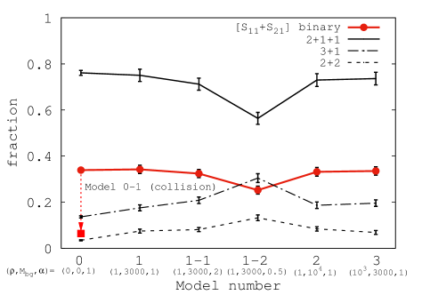
Figure 1 shows the outcome probabilities for all the models. The error bars indicate the Poisson uncertainties for each simulation set. A short description of the relevant model parameters (density , total background mass and ratio of the binding energies of the two initial binaries ; see Table 2) is provided below each model name. We use different line types for each outcome: the 2+1+1 outcome (thin black solid line), the 3+1 outcome (dot-dashed line) and the 2+2 outcome (dashed line). In addition, we indicate the formation probabilities of the most massive [] binaries by the thick solid red line with circular dots. Note that the fractions of the 2+1+1 outcome (black solid line) include those for the [] binary as well as all other possible 2+1+1 outcomes.
As shown in the figure, the 2+1+1 outcome is the most probable () across all the models (Model 0 to Model 3). Additionally, within this outcome, the [] binary is the most likely to form (), followed by the formation of the second most massive binaries, which are not shown in the figure. Note that since we consider two stars of equal mass (), two different binaries of the same mass, ([] or [] with ), could form. Their outcome probabilities are comparable ( for each binary). The outcome fractions of the least massive binaries ([] or [] with a mass ) are the lowest (). However, when we take into account physical collisions assuming finite sizes for the stars, the fraction of outcomes producing a [] binary (red square connected with the downward dotted arrow from the fraction for Model 0) is reduced to (decrease by a factor of 5-6). In reality, direct physical collisions during encounters could occur (Leigh & Geller, 2012, 2015) and their chances may increase in the presence of a background potential due to more gravitationally-focused cross sections for the stars and longer-lasting interactions accompanied by an increased probability of interruptions by other stars (Geller & Leigh, 2015). In all models, the 1+1+1+1 outcome has not emerged. Given the negative total energy in our simulations this is expected because the 1+1+1+1 outcome only forms when the total energy is positive.
Comparing Model 1 () with Models 1-1 and 1-2 (), we find that the fraction of 2+1+1 outcomes (including that for the [] binary) decreases whereas the fraction of 3+1 outcomes increases. These results are consistent with other studies (e.g Mikkola, 1984; Gualandris et al., 2004; Leigh et al., 2016). As the binding energy ratio becomes different from unity, the closer binary acts more like a single star causing the interaction to resemble more a three-body exchange encounter, leading to the preferential formation of triples. Given the different masses of the two initial binaries, the ratio between their semimajor axes becomes larger as decreases, or . In other words, the semimajor axis of the less massive initial binary () is smallest for . This seems to explain the larger increase in the fraction of 3+1 outcomes for , since the less massive initial binary effectively acts more like a single star in this case. We emphasize that a more thorough investigation focusing on the effects of adopting different mass ratios and binding energy ratios is required to confirm these conclusions.
We do not observe significant differences in the outcome probabilities between the various models (with/without the background potential and for different depths of the background potential). This is because in most of the simulations the stellar interactions tend to occur inside a region where the stellar dynamics are governed by the stellar gravitational potential, not by the background potential. Furthermore, the ejection velocities of the single stars tend to be sufficiently high that they are capable of escaping the background potential to infinity without being trapped in the background potential, which we show in Figure 7. This is consistent with the results of Ryu et al. (2017b). They performed numerical scattering experiments between two identical binaries in a homogeneous background potential, and investigated the effects of the potential as a function of its density and the semimajor axes of the two colliding binaries (see equation 17 in Ryu et al. 2017b). For tightly bound binaries () and the densities considered in this study, they showed that the outcomes are determined by stellar interactions taking place within a region where the stellar masses are larger than the enclosed background mass, corresponding to Region 1 in Ryu et al. (2017b).
| Model | (E,2E) | (NE,2E) | (E,1E) | (NE,1E) | (E,NE) | (NE,NE) |
|---|---|---|---|---|---|---|
| (unit) | ||||||
| 1 | 9.26 | 0.455 | 1.99 | 0 | 0 | |
| 1-1 | 9.55 | 0.327 | 1.19 | 0 | 0 | 0 |
| 1-2 | 8.73 | 0.900 | 3.77 | 0 | 0 | 0 |
| 2 | 8.24 | 1.31 | 4.15 | 3.19 | 0 | 0 |
| 3 | 4.46 | 4.15 | 4.62 | 83.1 | 0 | 9.23 |


A comparison with the branching ratios of GPZE04 (see their Figure 3) shows that we find predominantly consistent outcome fractions. On the one hand, they find an increase in the fraction of 3+1 outcomes as becomes different from unity, as shown in Figure 1. On the other hand, in our study, the 2+1+1 outcome for is the most probable, whereas in their study the most probable case is "Flybys" (if the two original binaries remain bound) followed by the 2+1+1 outcome ("Ionizations+ Orionis" in their Figure 3), which is a little bit lower ( for ) than in our simulations. However, since we are likely using different initial conditions such as impact parameters 888We miss many “flyby” outcomes in our simulations due to having adopted smaller collisional cross sections at impact. and initial separations, a direct comparison with their results is not straightforward.

3.1.2 Escape fraction
In contrast to the case with purely stellar interactions, ejected stars could be trapped in the background potential. In fact, only when the ejection velocities of the stars are sufficiently high can they escape the background potential to spatial infinity. In our simulations, we check at every time step whether or not stars have escaped from the potential. We assume that stars have escaped when they are spatially outside the potential and they are unbound from the potential, i.e.,
| (6) |
where is the total mass enclosed in a spherical volume of radius and is the velocity required by a star at to escape from the potential to spatial infinity.
For the 2+1+1 outcome, there are six possible scenarios depending on whether each binary and each single star could escape from the background potential,
-
1.
(E, 2E): both the binary (E) and the two single stars (2E) have escaped,
-
2.
(NE, 2E): the binary has not escaped (NE) whereas the two single stars have escaped,
-
3.
(N, 1E): the binary and only one single star (1E) have escaped,
-
4.
(NE, 1E): the binary has not escaped and only one single star (1E) has escaped,
-
5.
(E, NE): the binary has escaped whereas all single stars have not escaped (NE),
-
6.
(NE, NE): Neither the binary or the two single stars have escaped.
The first/second slot in the parentheses indicates whether binaries/single stars have escaped from the potential at . For notational succinctness, we also refer to binaries which have (have not) escaped as E-binary (NE-binary).
Figure 2 and Table 3 show the escape fractions for the cases listed above, and for each of the models with the background potential. The figure shows a clear trend in that as the escape velocity increases, a larger number of binaries remain trapped (solid line with hollow circles). In particular, in Model 3 with the largest escape velocity (see Table 2), since the typical ejection velocities of the binaries are comparable to the escape velocity of the potential, around 40% of the binaries could not escape; this fraction becomes comparable to that of the escaped binaries (E,2E). And it is also more likely in Model 3 that one single star stays trapped in the background potential, i.e., (E,1E) and (NE,1E), compared to the other models. From this we can see that the escape velocity may play a role as a good indicator to characterize the depth of the potential instead of only or .
In the following sections, we will present the distributions of the orbital parameters for the most massive binaries and the two single stars.
3.2 Statistical properties of the most massive binaries and the two ejected single stars
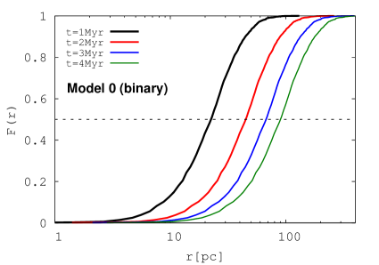
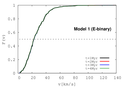
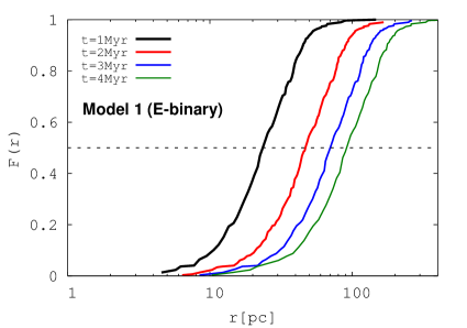
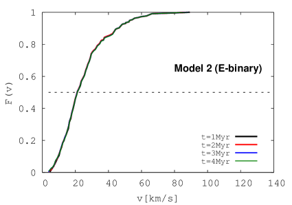
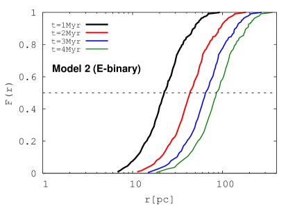
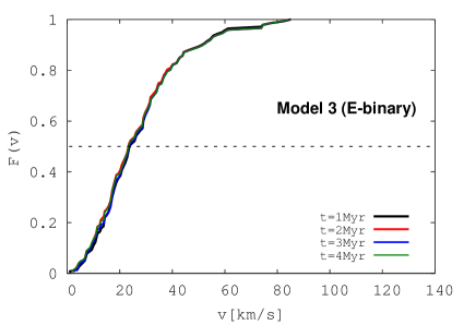
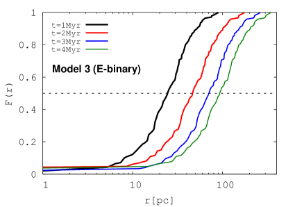
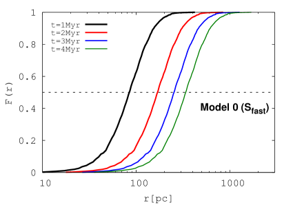
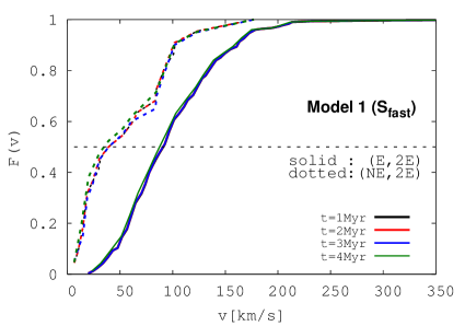
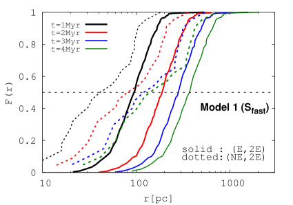
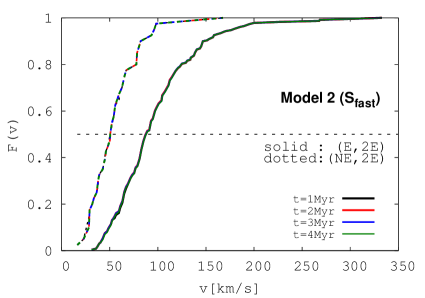
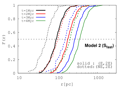
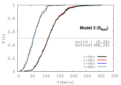
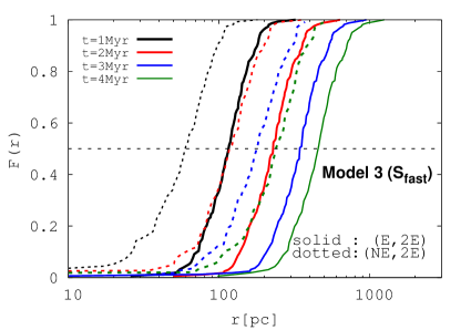
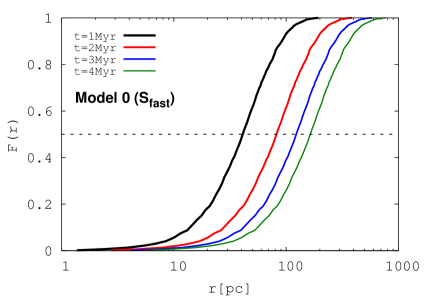
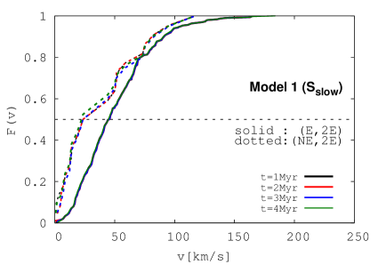
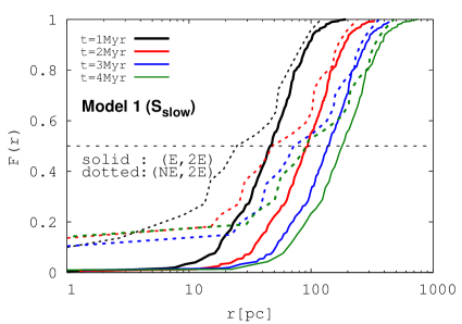
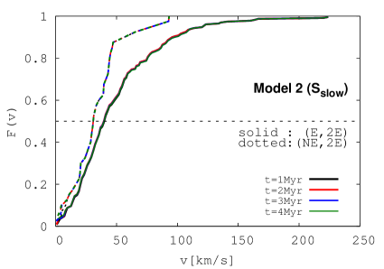
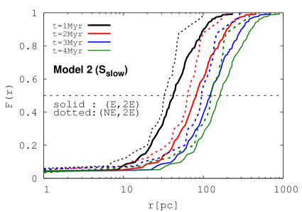
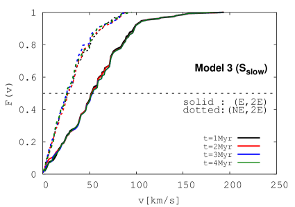
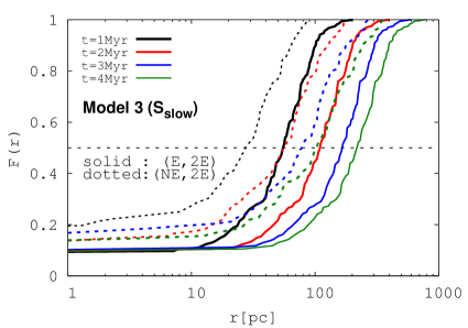
In this section we describe the statistical properties of the most massive binaries (i.e. those formed from []), and the two ejected stars produced by the scattering experiments. Namely, we provide the distributions of the semimajor axes and the eccentricities for the binaries, as well as the distributions of the final velocities for both the binaries and the ejected single stars. In addition to these, we also explore the ejection times and the relative angles between the stars. Since we could not find any statistically meaningful differences between Model 1 and Model 1-1, from now on, we shall primarily focus on the analysis of the results for Model 0, Model 1, Model 2 and Model 3. All the distributions shown in the following are made using the orbital parameters at for the cases where two single stars have escaped, unless indicated otherwise. We provide the cumulative distributions of radial distances from the system CM and the speeds at and for the escaped binaries (E-binaries) in Figure 14 in Appendix A.
3.2.1 The statistical properties of the final binaries
| Model (Figure) | 0 | 1 | 2 | 3 |
|---|---|---|---|---|
| (3) | 1.27 | 1.73 / 1.17 | 1.62 / 1.17 | 1.41 / 0.935 |
| (4) | 22.5 | 2.24 / 22.8 | 2.52 / 22.7 | 5.81 / 25.5 |
| (7) | 84.1 | 35.2 / 92.7 | 50.4 / 92.2 | 64.7 / 113 |
| (7) | 40.9 | 28.6 / 46.5 | 31.1 / 41.8 | 33.9 / 58.3 |
| (8) | 1.86 | 1.20 / 1.78 | 1.39 / 1.96 | 1.71 / 1.89 |
| (8) | 3.72 | 18.4 / 3.92 | 21.7 / 4.14 | 10.8 / 4.52 |
| (8) | 1.83 | 14.9 / 1.97 | 14.4 / 1.98 | 5.41 / 2.30 |
| [∘] ( 11, 12) | 111 | 109 | 105 | 89.1 |
| [∘] (11, 12) | 156 | 154 | 156 | 156 |
| [∘] (11,12) | 105 | 108 | 112 | 120 |
| (9) | - | 3.88 | 4.04 | 3.02 |
| (9) | - | 4.16 | 4.37 | 3.19 |
| (9) | - | 4.45 | 4.59 | 3.39 |
| (10) | - | 3.77 | 3.94 | 2.59 |
| (10) | - | 4.29 | 4.44 | 3.11 |
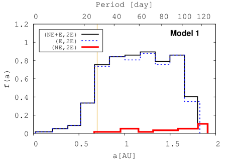
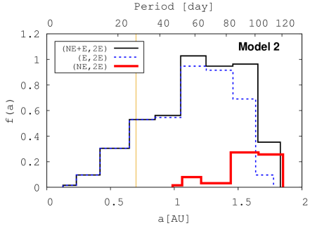
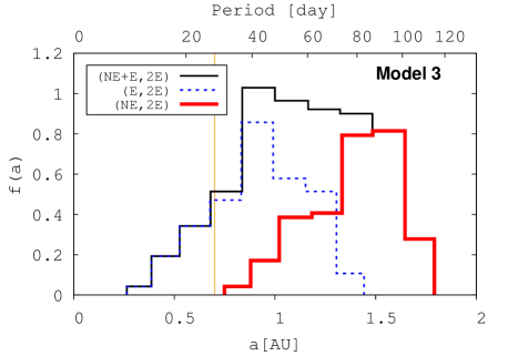
Figure 3 shows the distributions of the semimajor axes for the [] binaries. In the plots for Model 1 to Model 3, we show three different distributions with different line types: those for the binaries which have escaped from the potential before (dotted blue line), those which have not escaped and remain bound to the potential (thick red solid line), and the overall distributions (thin black solid lines) as the sum of the two distributions. The vertical gold lines indicate an observed value of or a period of 29 days (GPZE04).
We can see how, in going from Model 1 to Model 4, the population of final binaries splits into two separate populations, i.e., E-binaries and NE-binaries. The NE-binary population gradually emerges. This is because, as the background potential becomes deeper, the escape velocity increases and hence it gets harder for the stars to escape. The two populations become comparable in size in Model 3 (see right bottom panel and Table 3), hence contributing equally to the overall distribution. Given the different values in the peaks of the two populations, the overall distribution (thin black solid line) becomes broader. The median values of for Model 0 are . Those for (NE,2E) case (from Model 1 to Model 3) are and and for (E,2E) case and and . We present the all of the median values for the distributions for the binaries and the single stars in Table 4.
We also notice that the distributions of NE-binaries (red thick solid line) are located at larger than those of E-binaries. This can be understood in terms of conservation of energy along with the escape velocity. In general, when two single stars are ejected, the recoiled binary carries some kinetic energy. As the recoil velocity of the binary increases, given a fixed total energy, a larger reservoir of negative energy is left for the binary itself, implying a tighter binary. Correspondingly, the fact that binaries could not escape from the background potential means that the instantaneous velocities (or the kinetic energies) of the binaries at the last ejection event were not sufficiently high. Therefore, with smaller energy reservoirs given to the binaries, their semimajor axes are distributed at larger .



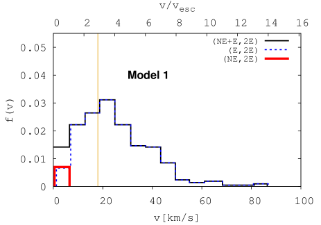
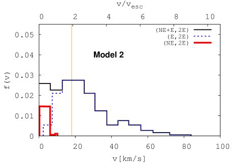
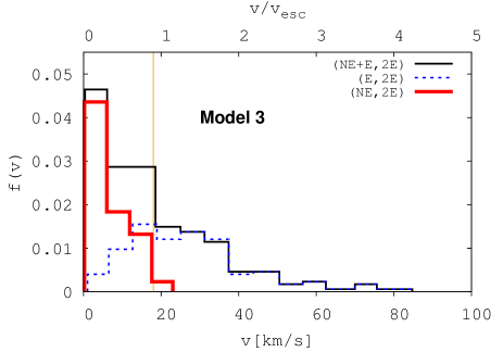
We find similar trends for the distributions of the final velocities shown in Figure 4, where the vertical gold lines indicate the observed value of . However, the velocity distributions of NE-binaries start to appear at small . Furthermore, we can see the overall shift of the distributions for E-binaries (blue dotted line) toward lower due to the gravitational pull from the potential as the binaries move outward. These two effects (the emergence of NE-binary populations at small and the overall shift of the velocity distribution for E-binaries to lower ) become more substantial as increases; finally, in Model 3, the shapes of the overall distributions have completely changed. The peak of the overall distribution for Model 3 has disappeared, turning into a more power-law-like distribution.
Using the velocity distributions for Model 0, we can understand the escape fractions shown in Section 3.1.2. If we make the rough assumption that the velocities at follow the distribution for Model 0, the escape probability for a background potential with can be written in terms of the cumulative distribution function of the velocities as,
| (7) |
where we have adopted (Model 1), (Model 2) and (Model 3) for and the maximum value of the final velocities of the binaries in Model 0 () for . Figure 5 shows calculated using Equation 7 with the velocity distribution for Model 0. The three vertical dotted lines indicate the escape velocities for Model 1 to Model 3 (from left to right). The probability at each escape velocity agrees well with the fractions given in Table 3.999Note that for more precise calculations, we have to consider the equation of motion in a harmonic potential with an upper bound of the integration in the numerator of to account for the energy required to travel from the centre to the potential boundary. We refer to Ryu et al. (2017a) for a more comprehensive analytical formulation of the 3-body outcomes. We show that the escape fractions are well explained using the results from Model 0, but this does not necessarily mean that all other results can be inferred from simulations without the background potential (Model 0). We find that in some cases stars cannot escape at their first ejections, but return back and go through multiple encounters with the remaining stellar systems in the potential. On the one hand, the escape fractions are not significantly affected by those cases because the single stars can manage to escape as they gain kinetic energy. On the other hand, this implies that the statistical properties of such single stars and binaries could be different compared to those from Model 0. Furthermore, for different choices of binary parameters (e.g. wide binaries) or different depths of the potential, the presence of the background potential could significantly change the properties of the final outcomes (Ryu et al., 2017b).
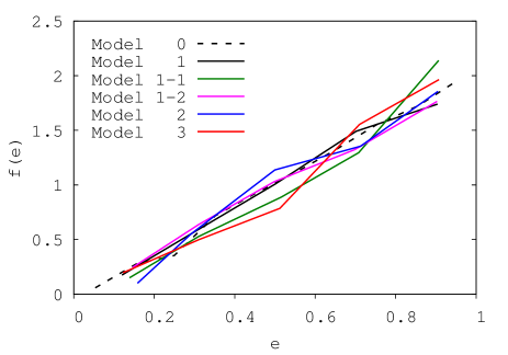
In Figure 6, we present the distributions of the eccentricities for all models. The eccentricity distributions approximately follow a thermally-averaged density function (Heggie, 1975), or:
| (8) |
which is typically found for eccentricity distributions in three-body scattering problems.
3.2.2 The statistical properties of the ejected single stars
In this section we present the statistical properties of the single stars, and in particular the distributions of the final velocities. As stars undergo chaotic interactions, all memory of the initial binaries (i.e., which objects comprised the initial binaries and ) may be lost. Therefore, given their identical masses, it is more appropriate to differentiate the single stars by their final speeds. Hence we refer to the ejected single stars with higher (lower) final speeds at the end of our simulations as (). We also use and for their speeds, respectively.
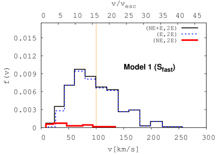
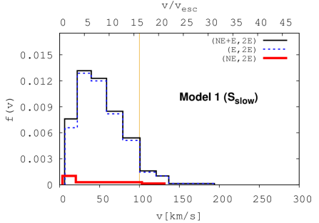
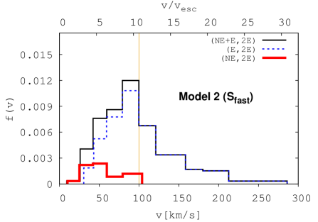
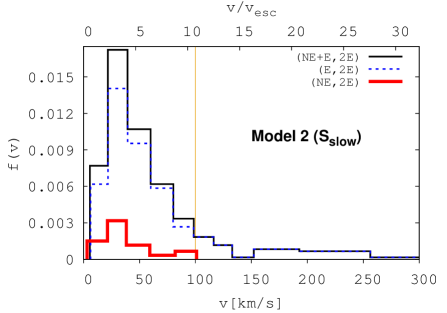
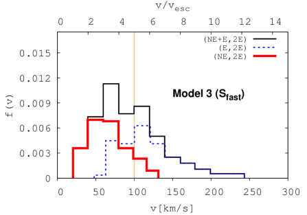
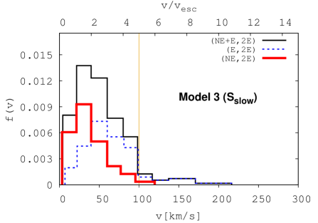
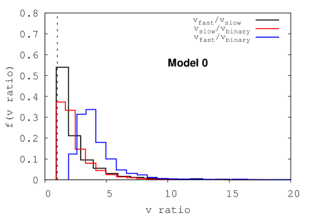
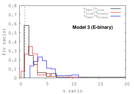
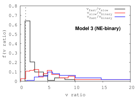
In Figure 7, we present the distributions of the final velocities for (left column) and (right column) for all models (from top to bottom), with the vertical gold lines indicating the observed value of . In all panels, the same colors are used as in Figure 3. In Figure 8, we compare the ratio of , and for Model 0 (upper panel) and Model 3 (E-binaries in the middle panel and NE-binaries in the lower panel). We only show those for Model 3 because the shapes and the median values are not significantly different from those for Model 1 and Model 2. We find from the figures that:
-
1.
The changes in shape of the distributions are not significant compared to the large changes in or . But we can still see that, as the background potential gets deeper (from top to bottom), the overall distributions become skewed toward low velocities due to the increasing contribution from the population of NE-binaries (red solid lines). Their median values for and for the models are given in Table 4.
-
2.
The velocities of and for the NE-binary cases are distributed at small . In general, for a single ejection event between a binary and a single star, a small kick of the binary (corresponding to the NE-binary case) translates into a small ejection velocity for the single star, because they are proportional to the mass ratio. However, for two ejection events (like 2+1+1), we have to take into account the vector sum of the two kicks to estimate the final kick of the binary (and hence the relative angles between them). There can be situations with two ejection events with wide relative angles where, even though each kick is very strong, the binary left behind has a smaller final kick velocity and remains bound to the potential. This could be one of the reasons for the extended high-end tail seen in the (NE,2E) distribution.
- 3.
-
4.
It is clearly seen that, as the potential becomes deeper, the distributions for the E-binary cases (blue dotted lines in Figure 7) decrease in size as the population of NE-binary cases emerges, but their shapes remain similar compared to the noticeable transformation in the velocity distributions of the binary (see (N,2E) distributions for Model 3 in Figure 4). This, along with the above, may imply that the motions of the single stars are not substantially affected by the background potential once they leave the potential. This is not surprising in light of the fact that the velocities of the rapidly-moving stars barely change because their kinetic energies are much larger than the background potential energy.
We show cumulative distributions of radial distances from the system CM and the speeds at and for (Figure 15) and (Figure 16) in Appendix A.
3.3 The escape time
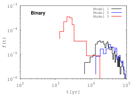
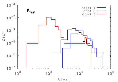
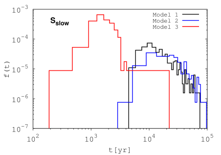
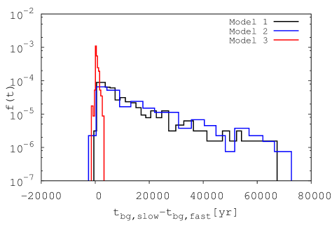
In Figure 9, we compare the distributions of the escape time for the final binaries (upper panel), for the faster star (middle panel), and for the slower star (bottom panel), for our background potential models. We define the escape time as the time (from the start of each simulation) taken by the stars to pass the outer boundary with speeds higher than the escape velocity . We only consider cases where both of the two single stars could escape (2E). For binaries which have not escaped until , we take . The distributions for such binaries are not shown in the figure.
The upper panel of Figure 9 shows that the escape time for Model 3 is more concentrated at small times compared to the other models. In order to gain a quantitative understanding of this, we introduce a characteristic time for the potential defined as follows,
| (9) |
where is the frequency of oscillation in a harmonic potential. This provides a good approximation to the "maximum" time taken for a star to arrive at the outer boundary from the origin with a velocity equal to the escape velocity. Notice that is a function of only , not or . Since in our simulations the last ejection events occur at shorter than , , we may ignore the duration of the stellar interactions for this analysis. We estimate that for Model 3 is shorter than for the other models by two orders of magnitude ( for and for ). From these estimates, we expect that the escape times for Model 3 with high are shorter, which is consistent with what is shown in the upper panel. In addition to that, indeed represents the peak value for Model 3 since typically the velocities of the binaries at 101010Note that it may be hard to infer at from the velocity distributions for Model 3 in Figure 4 since the velocities of the escaped binaries keep decreasing due to the gravitational pull from the potential (the distributions are for at ). are comparable to for . However, when the typical velocities of the binaries at are higher than the escape velocities, may overestimate the actual escape times. The distribution of for Model 2 is shifted towards longer compared to that for Model 1, which may appear contradictory to the estimates based on given their same densities. But for these two models is , lower than typical binary speeds at . For this case, the trend arises simply because the width of the potential is larger (larger ) for Model 3. See Table 4 for the median values of .
In the middle and bottom panels, we can see that the single stars show similar trends in the distributions to those of the binaries. But it is clear that, given the higher speeds of the single stars, for and are distributed at shorter times than that for the binaries, roughly shorter by the mass ratios between the single stars and the binary, namely, .
In Figure 10, we further show the distributions of for with respect to those for . Given the similar distributions for and , the resulting distributions for and extend down to (even to negative values). As shown in the figure, it is more likely that stars moving at higher speeds have escaped first.
3.4 The relative angles between the ejected objects
In this section, we study the relative angles between objects, i.e., single-single, single-binary. We expect that the statistical properties of the angles can provide observationally useful insight to identify runaway objects with a common origin.
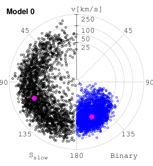
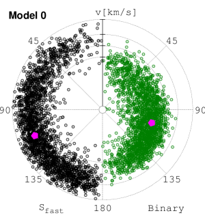
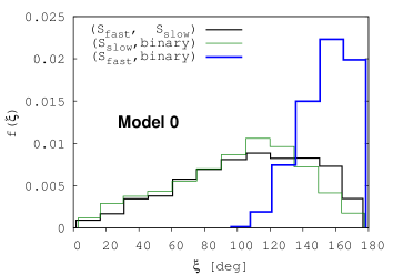
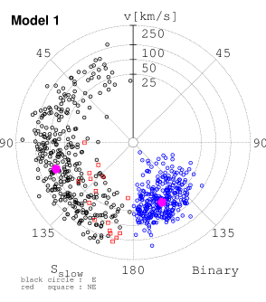
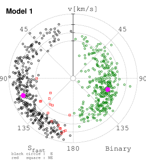
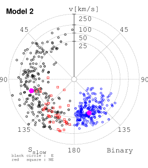
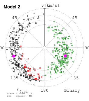
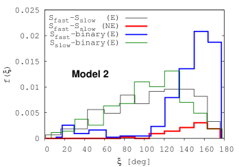
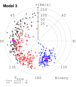
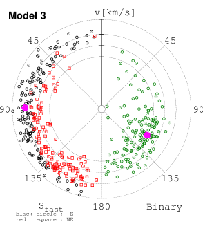
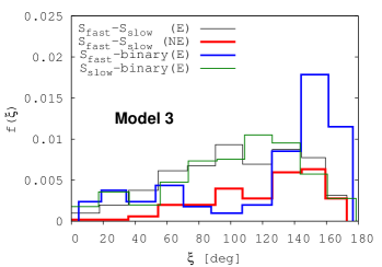
In Figure 11, we present the distributions of the relative angle as a function of the speeds for Model 0. Here, we define the relative angle as the relative angle between the velocity vectors of the two stars. In the first two circular plots, the distributions for are projected on to the () plane with the median values (magenta pentagon dots). The values for the single stars (the binaries) are marked in the left-half (right-half) of the circle. In particular, in the left panel, we present for and the binaries with respect to (so represents the speeds for and the binaries) while in the middle panel, we present for and the binaries with respect to (so and ). Each dotted circular grid (from the inner circle to the outer circle) indicates velocities of 25, 50, 100 and 250. The radial grids (from north to south) show separated by from to . In the right panel, we show the distribution function for . We have used the same colors for the same types of angles in all three panels. For example, the blue dots in the left panel refer to between and the binaries, which corresponds to the distribution with the blue line in the right panel.
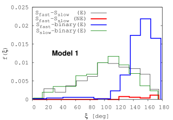
In Figure 12, we show the same distributions for the models with the background potential (Model 1 to Model 3). The same plot format and layout are used as in Figure 11. In these plots, different from Model 0, we make a distinction between cases where the binaries have escaped (E, marked with the black circles) and cases where the binaries have not escaped (NE, marked with the red squares).
There are several characteristic features found from the distributions for in both Figures 11 and 12.
-
1.
The relative angles between and the binaries (blue solid lines and blue dots) are densely distributed at with peaks near .
-
2.
For cases with NE-binaries in Figure 12, the relative angles between the two single stars are more concentrated at higher (red square dots). In addition, as the escape velocity increases (from Model 1 to Model 3), the red dots spread out over a wider range in .
-
3.
The relative angles for and the binaries with respect to are broadly distributed (black/green dots and lines) compared to the distribution for between and the binaries (blue lines and dots), but more biased toward higher values of with peaks at .
Those features above can be understood in terms of the relation between the recoil velocities of the binaries and the relative angle between the two single stars. If the two single stars are ejected with a wider angle (large ), it is more likely that the binary gets a smaller recoil kick. As an extreme case, when two single stars are ejected at the same speed in opposite directions (or ), the final recoil velocity of the binary sums to zero (as a result of the two kicks in opposite directions) so that it remains where the last ejection event occurred.
We find feature 1 in our simulations as a result of the fact that kicks from more rapidly-moving stars tend to contribute more to the final recoil velocity of the binary than slowly moving stars. In order to better understand this feature quantitatively, we use Equation 27 from Ryu et al. (2017a) (with ), which relates the speeds of the binary to the relative angle between the two single stars in a harmonic potential. The equation gives the relative angles between and at the outer boundary of the potential as follows,
| (10) |
where (=binary, or ) 111111Here, is the speed at .. However, in deriving this equation, the binary and the ejected single star are only distinguished by their masses. Therefore, the relative angles between and the binary can be estimated by exchanging with . Expressing in terms of the momenta,
| (11) |
We can first see that since the numerator is negative. Note that the case for corresponds to Model 0. In particular, for binaries and single stars which have escaped from the background potential, and given the velocity distributions for the binaries (Figure 4) and the single stars (Figure 7) and their ratio (Figure 8), we can roughly estimate that and .
In order to interpret feature 2, we introduce the maximum angle between two single stars required to give a sufficiently high recoil kick to a binary that the binary can escape to infinity. In other words, if two single stars are ejected with at their given speeds, the final binary will not gain enough kinetic energy to completely escape. Therefore, we expect that for the NE-binary cases should be distributed at . We note that is a function of the speeds of the two single stars () and the escape velocity , namely, .
Using , we can understand feature 2 and try to provide useful insight from an observational perspective. Using Equation 10 (or Equation 36 in Ryu et al. 2017a with ), we impose the condition that at and , . More explicitly,
| (12) |
Again, the term on the left-hand side represents the final momentum of the binary at the last ejection event and the term on the right-hand side the minimum momentum of the binary necessary to travel from the origin to the outer boundary of the potential, and subsequently to spatial infinity.
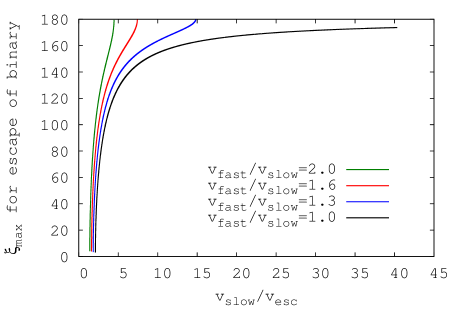
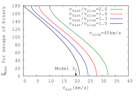
In the upper panel of Figure 13, we estimate (using Equation 12) as a function of in units of for various ratios of (see Figure 8). As shown in the figure, increases rapidly at . It reaches at typical velocities for found in Model 1 and 2 (median velocities of ) for all speed ratios, which explains well the feature 2. However, considering smaller values for in Model 3, it is hard to read from the upper panel. Hence we additionally provide a plot (bottom panel), which shows as a function of assuming . We can see that for in Model 3 (indicated with the downward arrow), decreases down to , which accounts for the wide range of dots in Figure 12, or feature 2.
From an observational perspective, we expect that the analytic relations above (as derived in the analytic paper) and the statistical properties of the relative angles found from our simulations can help restrict the region in parameter space where we need to look in order to find an unknown related object given observations of some other runaway stars. Note that, in the derivation of the above relation, the three bodies are only identified by their masses, meaning that the relation can be applied to any kind of isolated system that evolves to produce 3-body outcomes (two ejected systems and one left-over system), not necessarily only to the 2+1+1 outcome.
4 Discussion and Summary
We have investigated the formation of runaway stars during binary - binary encounters in a background potential via dynamical ejections. To this end, we have performed numerical scattering experiments for various potential models, under the assumption that the potential remains static in time. In order to understand the effects of the background potential on the statistical properties of the outcomes, we explored a range of different depths for the potential: () = (0, 0, 0) for Model 0, (1, ) for Model 1, (1, ) for Model 2 and (1000, ) for Model 3. The parameters of the models are summarized in Table 2.
We have found that, for encounters of two tightly bound binaries, the background potential does not have an appreciable effect on the outcome formation probabilities. However, in the presence of the potential, two distinctive populations of binaries, with different orbital properties, emerge depending on whether they could escape or not. Upon analyzing our results, we have shown that the escape velocity of the potential can play a role as a good indicator to identify these two populations. We also found that the relative angles between stars have a dependence on the depth of the potential, or the escape velocity.
We summarize the effects of the background potential as follows:
-
1.
We find that for the encounters of two tightly bound binaries, the outcome fractions have no appreciable dependence on the depth of the background potential. This is because the stellar interactions take place where the mutual gravitational potentials between stars are dominant over the gravitational background potential. Additionally, during the interactions, the ejection velocities of single stars are typically higher than the escape velocities from the background potential so they easily escape. However, for encounters involving wide binaries with low ejection velocities, they may experience subsequent interactions while they are oscillating inside the potential (Ryu et al., 2017b).
-
2.
As the background potential deepens, a larger number of binaries cannot escape (NE-binaries), resulting in the emergence of two distinct populations of binaries. When the escape velocities are comparable to the typical velocities of the binaries (see Figure 4) as in Model 3, , around 40% of the binaries cannot escape, almost the same fraction as that of the escaped binaries (E-binaries). More importantly, these two populations have different orbital parameters: the semimajor axes of the escaped binaries tend to be shorter. Their velocity distributions extend up to whereas the velocities for are limited by the escape velocities. Additionally, as the potential gets deeper, the gravitational pull from the potential more significantly slows down the binaries, resulting in a shift of the velocity distributions for the escaped binaries towards lower . Here, we emphasize that the escape velocity plays a role as a good measure to gauge the effects of the background potential.
-
3.
In contrast with the binaries, we could not find any noticeable effects of the background potential on the velocities of the ejected single stars. This is essentially due to the fact that the velocities of the rapidly-moving stars barely change because their kinetic energies are much larger than the background potential energy.
-
4.
We find that the escape times (the time taken for stars to cross the potential boundary from the onset of the encounter) for Model 1 and Model 2 are and that for Model 3 is around a few . From the difference in the escape times between the two single stars, we confirm that it is more likely that stars ejected at higher speeds are the ones to escape first.
-
5.
The relative angles between stars (-, - binary and - binary) are generally large, independent of the presence of the background potential. More interestingly, the angle between and the binary (blue circles in Figure 11 and Figure 12) is mostly concentrated at , while the values between and when the final binaries remain bound to the potential (red squares in in Figure 11 and Figure 12) are distributed at larger . Moreover, the distributions stretch out over a wider range of as the potential gets deeper. We have explained these trends using the term defined in Equation 12.
-
6.
In summary, we have discussed the effects of a background potential on the formation of runaway stars and the statistical properties of the orbital parameters. We find that in the presence of the background potential, the outcomes have different orbital properties depending on whether or not they have escaped from the potential. From our study, we find that stars moving faster than the escape velocities, as is the case for runaway stars, are less affected by the background potential. Furthermore, we find some constraints on the relative angles between the ejected objects, which we expect to be observationally useful for identifying related runaway stars.
Acknowledgements
Results in this paper were obtained using the high-performance LIred computing system at the Institute for Advanced Computational Science at Stony Brook University, which was obtained through the Empire State Development grant NYS #28451.
References
- Andersen et al. (2009) Andersen M., Zinnecker H., Moneti A., McCaughrean M. J., Brandl B., Brandner W., Meylan G., Hunter D., 2009, ApJ, 707, 1347
- Blaauw (1961) Blaauw A., 1961, Bull. Astron. Inst. Netherlands, 15, 265
- Blaauw & Morgan (1954) Blaauw A., Morgan W. W., 1954, ApJ, 119, 625
- Capuzzo-Dolcetta & Fragione (2015) Capuzzo-Dolcetta R., Fragione G., 2015, M.N.R.A.S., 454, 2677
- Erwin (1969) Erwin F., 1969, NASA Technical Report, 315, 1
- Fragione & Capuzzo-Dolcetta (2016) Fragione G., Capuzzo-Dolcetta R., 2016, M.N.R.A.S., 458, 2596
- Fragione et al. (2017) Fragione G., Capuzzo-Dolcetta R., Kroupa P., 2017, M.N.R.A.S., 467, 451
- Fregeau et al. (2004) Fregeau J. M., Cheung P., Portegies Zwart S. F., Rasio F. A., 2004, M.N.R.A.S., 352, 1
- Geller & Leigh (2015) Geller A. M., Leigh N. W. C., 2015, ApJL, 808, L25
- Gies & Bolton (1986) Gies D. R., Bolton C. T., 1986, ApJ Supp., 61, 419
- Gualandris et al. (2004) Gualandris A., Portegies Zwart S., Eggleton P. P., 2004, M.N.R.A.S., 350, 615
- Heggie (1975) Heggie D. C., 1975, M.N.R.A.S., 173, 729
- Herbig & Terndrup (1986) Herbig G. H., Terndrup D. M., 1986, ApJ, 307, 609
- Hoogerwerf et al. (2000) Hoogerwerf R., de Bruijne J. H. J., de Zeeuw P. T., 2000, ApJL, 544, L133
- Hunter et al. (1995) Hunter D. A., Shaya E. J., Holtzman J. A., Light R. M., O’Neil Jr. E. J., Lynds R., 1995, ApJ, 448, 179
- Kenyon et al. (2014) Kenyon S. J., Bromley B. C., Brown W. R., Geller M. J., 2014, ApJ, 793, 122
- Leigh & Geller (2012) Leigh N., Geller A. M., 2012, M.N.R.A.S., 425, 2369
- Leigh & Geller (2015) Leigh N. W. C., Geller A. M., 2015, M.N.R.A.S., 450, 1724
- Leigh et al. (2016) Leigh N. W. C., Stone N. C., Geller A. M., Shara M. M., Muddu H., Solano-Oropeza D., Thomas Y., 2016, M.N.R.A.S., 463, 3311
- Mikkola (1984) Mikkola S., 1984, M.N.R.A.S., 207, 115
- Oh et al. (2015) Oh S., Kroupa P., Pflamm-Altenburg J., 2015, ApJ, 805, 92
- Perets & Šubr (2012) Perets H. B., Šubr L., 2012, ApJ, 751, 133
- Pfalzner (2009) Pfalzner S., 2009, A&A, 498, L37
- Portegies Zwart et al. (2010) Portegies Zwart S. F., McMillan S. L. W., Gieles M., 2010, Ann. Rev. A&A, 48, 431
- Poveda et al. (1967) Poveda A., Ruiz J., Allen C., 1967, Boletin de los Observatorios Tonantzintla y Tacubaya, 4, 86
- Ryu et al. (2016) Ryu T., Tanaka T. L., Perna R., 2016, M.N.R.A.S., 456, 223
- Ryu et al. (2017a) Ryu T., Leigh N. W. C., Perna R., 2017a, preprint, (arXiv:1703.08538)
- Ryu et al. (2017b) Ryu T., Leigh N. W. C., Perna R., 2017b, M.N.R.A.S., 467, 4447
- Selman & Melnick (2013) Selman F. J., Melnick J., 2013, A&A, 552, A94
- Stone (1979) Stone R. C., 1979, ApJ, 232, 520
- Turon et al. (1992) Turon C., et al., eds, 1992, The HIPPARCOS input catalogue ESA Special Publication Vol. 1136
- Zwicky (1957) Zwicky F., 1957, Morphological astronomy
Appendix A The Cumulative distributions at and .
We provide the cumulative distributions of the spatial distances from the system CM and the speeds for the escaped binaries (Figure 14), (Figure 15) and (Figure 16) for all models for and .

