∎ ∎
Department of Electrical Engineering (ESAT-STADIUS) - KU Leuven, Kasteelpark Arenberg 10, 3001 Leuven, Belgium.
22email: masoud.ahookhosh@kuleuven.be 33institutetext: F.J. Aragón Artacho 44institutetext: Department of Mathematics, University of Alicante, Spain. 44email: francisco.aragon@ua.es 55institutetext: R.M.T. Fleming 66institutetext: Systems Biochemistry Group, Luxembourg Center for Systems Biomedicine, University of Luxembourg, Campus Belval, 4362 Esch-sur-Alzette, Luxembourg. 66email: ronan.mt.fleming@gmail.com 77institutetext: P.T. Vuong 88institutetext: Systems Biochemistry Group, Luxembourg Center for Systems Biomedicine, University of Luxembourg, Campus Belval, 4362 Esch-sur-Alzette, Luxembourg.
Faculty of Mathematics, University of Vienna, Oskar-Morgenstern-Platz 1, 1090 Vienna, Austria.
88email: vuong.phan@univie.ac.at
Local convergence of the Levenberg–Marquardt method under Hölder metric subregularity††thanks: F.J. Aragón was supported by MINECO of Spain and ERDF of EU, as part of the Ramón y Cajal program (RYC-2013-13327) and the I+D grant MTM2014-59179-C2-1-P. M. Ahookhosh, R.M.T. Fleming, and P.T. Vuong were supported by the U.S. Department of Energy, Offices of Advanced Scientific Computing Research and the Biological and Environmental Research as part of the Scientific Discovery Through Advanced Computing program, grant #DE-SC0010429. P.T. Vuong was also supported by the Austrian Science Foundation (FWF), grant I 2419-N32.
Abstract
We describe and analyse Levenberg–Marquardt methods for solving systems of nonlinear equations. More specifically, we propose an adaptive formula for the Levenberg–Marquardt parameter and analyse the local convergence of the method under Hölder metric subregularity of the function defining the equation and Hölder continuity of its gradient mapping. Further, we analyse the local convergence of the method under the additional assumption that the Łojasiewicz gradient inequality holds. We finally report encouraging numerical results confirming the theoretical findings for the problem of computing moiety conserved steady states in biochemical reaction networks. This problem can be cast as finding a solution of a system of nonlinear equations, where the associated mapping satisfies the Łojasiewicz gradient inequality assumption.
Keywords:
Nonlinear equation Levenberg–Marquardt method Local convergence rate Hölder metric subregularity Łojasiewicz inequalityMSC:
65K05 65K10 90C26 92C421 Introduction
For a given continuously differentiable mapping , we consider the problem of finding a solution of the system of nonlinear equations
| (1) |
We denote by the set of solutions of this problem, which is assumed to be nonempty. Systems of nonlinear equations of type (1) frequently appear in the mathematical modelling of many real-world applications in the fields of solid-state physics Eilenberger , quantum field theory, optics, plasma physics hasegawa_plasma_1975 , fluid mechanics Whitham , chemical kinetics artacho_globally_2014 ; artacho_accelerating_2015 , and applied mathematics including the discretisation of ordinary and partial differential equations ortega_iterative_2000 .
A classical approach for finding a solution of (1) is to search for a minimiser of the nonlinear least-squares problem
| (2) |
where denotes the Euclidean norm. This is a well-studied topic and there are many iterative schemes with fast local convergence rates (e.g., superlinear or quadratic) such as Newton, quasi-Newton, Gauss–Newton, adaptive regularised methods, and the Levenberg–Marquardt method. When , to guarantee fast local convergence, these methods require an initial point to be sufficiently close to a solution , and the matrix gradient of at (i.e., the transpose of the Jacobian matrix), denoted by , to be nonsingular (i.e., full rank), cf. BelCGMT ; fischer2015globally ; nocedal_numerical_2006-1 ; ortega_iterative_2000 ; Yuan2015 .
The Levenberg–Marquardt method is a standard technique used to solve the nonlinear system (1), which is a combination of the gradient descent and the Gauss–Newton methods. More precisely, in each step, for a positive parameter , the convex subproblem
with given by
| (3) |
is solved to compute a direction , which is the unique solution to the system of linear equations
| (4) |
where denotes the identity matrix. By choosing a suitable parameter , the Levenberg–Marquardt method acts like the gradient descent method whenever the current iteration is far from a solution , and behaves similar to the Gauss–Newton method if the current iteration is close to . The parameter helps to overcome problematic cases where is singular, or nearly singular, and thus ensures the existence of a unique solution to (4), or avoids very large steps, respectively. For , the Levenberg–Marquardt method is known to be quadratically convergent to a solution of (1) if is nonsingular. In fact, the nonsingularity assumption implies that the solution to the minimisation problem (2) must be locally unique, see bellavia_strong_2015 ; kanzow_levenbergmarquardt_2004 ; alefeld_rate_2001 . However, assuming local uniqueness of the solution might be restrictive for many applications.
The notion of (local) error bound usually plays a key role in establishing the rate of convergence of the sequence of iterations generated by a given algorithm. This condition guarantees that the distance from the current iteration to the solution set , denoted by , is less than the value of a residual function at that point (). The earliest publication using error bounds for solving a linear inequality system is due to Hoffman Hoffman_1952 , which was followed by many other authors, especially in optimisation. For more information about error bounds, we recommend the nice survey Pang_1997 .
For the particular case of nonlinear systems of equations, Yamashita and Fukushima alefeld_rate_2001 proved the local quadratic convergence of the Levenberg–Marquardt method with assuming a local error bound condition. More precisely, they assumed metric subregularity of around , which entails the existence of some constants and such that
| (5) |
where denotes the closed ball centered at with radius . In this case, the residual function is given by . In those situations where the value of is known, the condition can be used as a stopping criterion for an iterative scheme, as it entails that the iterations must be close to a solution of (1).
Let us emphasise that, for , the nonsingularity of implies that is locally unique and that (5) holds. Indeed, by the Lyusternik–Graves theorem (see, e.g., (DontchevRockafellar2014, , Theorem 5D.5), (Mordukhovich2006, , Theorem 1.57), or (CDK18, , Proposition 1.2)), the nonsingularity of is equivalent to the strong metric regularity of at , which implies strong metric subregularity of at . However, the latter does not imply the nonsingularity assumption and allows the solutions to be locally nonunique. This means that metric subregularity is a weaker assumption than the nonsingularity. In fact, for possibly different than , strong metric subregularity of at is equivalent to surjectivity of (see, e.g., (CDK18, , Proposition 1.2 and Theorem 2.6)). The successful use of the local error bound has motivated many researchers to investigate, under assumption (5), the local convergence of trust-region methods Fan2006 , adaptive regularised methods bellavia_strong_2015 , and the Levenberg–Marquardt method behling_effect_2013 ; fan_modified_2012 ; fan_quadratic_2005 , among other iterative schemes.
The main motivation for this paper comes from a nonlinear system of equations, the solution of which corresponds to a steady state of a given biochemical reaction network, which plays a crucial role in the modeling of biochemical reaction systems. These problems are usually ill-conditioned and require the application of the Levenberg–Marquardt method. As we numerically show in Section 4, is usually rank deficient at the solutions of (1). During our study of the properties of this problem, we were not able to show that the metric subregularity condition (5) is satisfied. However, taking standard biochemical assumptions artacho_accelerating_2015 , we can show that the corresponding merit function is real analytic and thus satisfies the Łojasiewicz gradient inequality and is Hölder metrically subregular around the solutions.
The local convergence of a Levenberg–Marquardt method under Hölder metric subregularity has been recently studied in Guo2015 ; ZhuLin16 . Nonetheless, the standard rules for the regularisation parameter have a very poor performance when they are applied for solving the nonlinear equation arising from the biochemical reaction network systems, as we show in a numerical experiment in Section 4. This motivated our quest to further investigate an adaptive Levenberg–Marquart method under the assumption that the underlying mapping is Hölder metrically subregular.
From the definition of the Levenberg–Marquardt direction in (4), we observe that a key factor in the performance of the Levenberg–Marquardt method is the choice of the parameter , cf. izmailov2014newton ; Kelley1 . Several parameters have been proposed to improve the efficiency of the method. For example, Yamashita and Fukushima alefeld_rate_2001 took , Fischer fischer2002local used , while Fan and Yuan fan_quadratic_2005 proposed with . Ma and Jiang MJ07 proposed a convex combination of these two types of parameters, namely, for some constant . In a subsequent work, Fan and Pan fan_pan proposed the more general choice , where is updated by a trust-region technique, and is a positive function such that , with . Inspired by these works, and assuming that the function is Hölder metrically subregular of order and its gradient is Hölder continuous of order , in this paper we consider an adaptive parameter of the form
| (6) |
where , and , for some constants and such that .
In our first main result, Theorem 3.1, we provide an interval depending on and where the parameter must be chosen to guarantee the superlinear convergence of the sequence generated by the Levenberg–Marquardt method with the adaptive parameter (6). In our second main result, Theorem 3.2, under the additional assumption that the merit function defined in (2) satisfies the Łojasiewicz gradient inequality with exponent , we prove local convergence for every parameter smaller than a constant depending on both and . As a consequence, we can ensure local convergence of the Lebenverg–Marquardt algorithm to a solution of (1) for all the above-mentioned biochemical networks as long as the parameter is chosen sufficiently small. To the best of our knowledge, this is the first such algorithm able to reliably handle these nonlinear systems arising in the study of biological networks. We successfully apply the proposed algorithm to nonlinear systems derived from many real biological networks, which are representative of a diverse set of biological species.
The remainder of this paper is organised as follows. In the next section, we particularise the Hölder metric subregularity for nonlinear equations and recall the Łojasiewicz inequalities. We investigate the local convergence of the Levenberg–Marquardt method under these conditions in Section 3. In Section 4, we report encouraging numerical results where nonlinear systems, arising from biochemical reaction networks, were quickly solved. Finally, we deliver some conclusions in Section 5.
2 Hölder metric subregularity and Łojasiewicz inequalities
Let us begin this section by recalling the notion of Hölder metric subregularity, which can be also defined in a similar manner for set-valued mappings (see, e.g., kruger_error_2015 ; CDK18 ).
Definition 1
A mapping is said to be Hölder metrically subregular of order around with if there exist some constants and such that
For any solution of the system of nonlinear equations (1), the Hölder metric subregularity of around reduces to
| (7) |
Therefore, this property provides an upper bound for the distance from any point sufficiently close to the solution to the nearest zero of the function.
Hölder metric subregularity around is also called Hölderian local error bound ngai_global_2015 ; vui_global_2013 . It is known that Hölder metric subregularity is closely related to the Łojasiewicz inequalities, which are defined as follows.
Definition 2
Let be a function defined on an open set , and assume that the set of zeros is nonempty.
-
(i)
The function is said to satisfy the Łojasiewicz inequality if for every compact subset , there exist positive constants and such that
(8) -
(ii)
The function is said to satisfy the Łojasiewicz gradient inequality if for any critical point , there exist constants and such that
(9)
Stanisław Łojasiewicz proved that every real analytic function satisfies these properties lojasiewicz1965ensembles . Recall that a function is said to be real analytic if it can be represented by a convergent power series. Fortunately, real analytic functions frequently appear in real world application problems. A relevant example in biochemistry is presented in Section 4.
Fact 1 ((lojasiewicz1965ensembles, , pp. 62 and 67))
Every real analytic function satisfies both the Łojasiewicz inequality and the Łojasiewicz gradient inequality.
Clearly, if the merit function satisfies the Łojasiewicz inequality (8), then the mapping satisfies (7) with and ; i.e., is Hölder metrically subregular around of order . In addition, if satisfies the Łojasiewicz gradient inequality (9), then for any and , it holds
The Łojasiewicz gradient inequality has recently gained much attention because of its role for proving the convergence of various numerical methods (e.g., BDL07 ; AB09 ; ABS13 ; artacho_accelerating_2015 ). The connection between this property and metric regularity of the set-valued mapping on an adequate set was revealed in BDLM10 , where it was also applied to deduce strong convergence of the proximal algorithm.
In some cases, for example when is a polynomial with an isolated zero at the origin, an order of the Hölder metric subregularity is known gwozdziewicz_lojasiewicz_1999 ; kurdyka_separation_2014 ; li_holder_2012 .
Fact 2 ((gwozdziewicz_lojasiewicz_1999, , Theorem 1.5))
Let be a polynomial function with an isolated zero at the origin. Then is Hölder metrically subregular around of order , where denotes the degree of the polynomial function .
The next example shows that the Powell singular function, which is a classical test function for nonlinear systems of equations, is not metrically subregular around its unique solution but is Hölder metrically subregular there. In addition, it demonstrates that the order given by Fact 2 is, in general, far from being tight.
Example 1
The Powell singular function more_1981 , which is the function given by
is (strongly) Hölder metrically subregular around but does not satisfy the metric subregularity condition (5). We have and is singular; thus, is not metrically regular around . Further, to prove that (5) does not hold, consider the sequence defined by . We see that and
Since we conclude that (5) does not hold.
Consider the polynomial function of degree , which satisfies . It follows from Fact 2 that there exist some constants and such that
This implies that is Hölder metrically subregular of order around . Nonetheless, the order given by Fact 2 can be improved by using the theory of -regularity: the function turns out to be -regular at , which implies by (izmailov2001, , Theorem 4) that (7) holds with (see also (izmailov2001, , Remark 7)). Recall that a twice differentiable mapping is said to be 2-regular at the point if the range of is for all , where is defined for by
is the projector in onto the complementary subspace to the range of , and stands for the second-order (Fréchet) derivative.
Indeed, for any , one has , so the range of is , whose complementary subspace is . Then, and for each , one has
which is full-rank for all . Therefore, the range of is equal to for all , and the function is -regular at .
There are many examples of smooth functions that are Hölder metrically subregular of order around some zero of the function and whose gradient is not full row rank at that point, cf. izmailov2001 ; izmailov2002 . Nonetheless, the following result restricts the possible values of : if is an isolated solution in (i.e., the function is Hölder strongly metrically subregular at , cf. Mordukhovich2015 ; CDK18 ), and is Lipschitz continuous around then one must have if . In fact, only Hölder continuity of is needed. Recall that a function is said to be Hölder continuous of order with constant around some point whenever there exist a positive constant such that
When , is said to be Lipschitz continuous with constant around .
Proposition 1
Let be a continuously differentiable function which is Hölder metrically subregular of order around some isolated solution . Assume further that is Hölder continuous around of order and that is not full row rank. Then, it holds that .
Proof
Because of the Hölder continuity assumption and the mean value theorem, there are some positive constants and such that, for all , it holds
| (10) |
By using the fact that is an isolated solution, it is possible to make smaller if needed so that (7) holds and
Since is not full row rank, there exists some such that . Consider now the points
Observe that
As for all , we deduce
Thus, we get
which implies that , since , as claimed.∎
The next example shows that the full rank assumption in Proposition 1 is not redundant, and that the upper bound can be attained.
Example 2
Consider the continuously differentiable functions given for by and , whose solution sets are and , respectively. Let . Then, and , which are both Hölder continuous around of order . Observe that while . Hence, it follows that is (Hölder) metrically subregular around of order , while it is easy to check that is Hölder metrically subregular around of order .
3 Local convergence of the Levenberg–Marquardt method
In this section, to solve a nonlinear system of the form (1), we consider an adaptive Levenberg–Marquardt method and investigate its local convergence near a solution. Specifically, we consider the following Levenberg–Marquardt algorithm.
In order to prove the local convergence of algorithm 1 to some solution , we assume throughout the paper that the next two conditions hold:
- (A1)
-
There exists some constants , , and such that the function is continuously differentiable and Lipschitz continuous with constant on , and is Hölder metrically subregular of order around ; that is, (7) holds.
- (A2)
-
is Hölder continuous of order with constant on .
Let us define the constants
and
We begin our study with an analysis inspired by alefeld_rate_2001 , fischer2002local and Guo2015 . The following result provides a bound for the norm of the direction based on the distance of the current iteration to the solution set . This will be useful later for deducing the rate of convergence of 1.
Proposition 2
Proof
For all , we will denote by a vector in such that . Since we have
which implies . Further,
| (13) |
Observe that is strongly convex and the global minimiser of is given by (4). Then, we have
| (14) |
From the definition of in (3), by (11) and (14), we deduce
| (15) |
Remark 1
If , by (16), we have that implies whenever is sufficiently close to .
The next result provides an upper bound for the distance of to the solution set based on the distance of to .
Proposition 3
If , assume that . Let and be two consecutive iterations generated by 1 with . Then, if , we have
| (18) |
where is a positive constant and
| (19) |
Proof
Let be such that . From the definition of in (3) and the reasoning in (15), we obtain
It follows from (A1) that there exists some constant such that for all . Then, by the definition of in (6) and the Lipschitz continuity of , we have that
| (20) |
which implies, thanks to (13),
where . By (7), (11), the latter inequality and Proposition 2, we get
where
Therefore,
with given by (19) and , giving the result.∎
The following proposition gives a different value of the exponent in (18).
Proposition 4
Assume that . Let and be two consecutive iterations generated by 1 with and such that . Then, there exists a positive constant such that
| (21) |
where
| (22) |
Proof
Let be such that and . Assume that (otherwise, the inequality trivially holds). By (11), we have
Thus, by the Cauchy–Schwarz inequality and (7), we get
that is,
| (23) |
Now, by (4), we have
| (24) |
By (A1) and Proposition 2, it holds,
It follows from (A1) that there exists some constant such that for all . Then, by the definition of in (6) and (A1), we get (20). Hence, by (24) and Proposition 2, we deduce
where and . Therefore, by (23),
| (25) |
Since , we have by (17) that
Finally, by (25), we deduce
whence,
where and . Since the expression for coincides with (22), the proof is complete.∎
Remark 2
(i) The bounds given by (18) and (21) are usually employed to analyse the rate of convergence of the sequence generated by 1. Observe that the values of and when are greater or equal than their respective values when . A larger value of or would serve us to derive a better rate of convergence. To deduce a convergence result from Proposition 3, one needs to have . This holds if and only if and , which imposes an additional requirement on the value of (to have a nonempty interval). For instance, when , one must have if and if . On the other hand, to guarantee that , a stronger requirement would be needed, namely, and . Nonetheless, it is important to observe that if one has that when , while only if and . Therefore, if , we can derive from Proposition 4 the quadratic convergence of the sequence for , which can only be guaranteed for by Proposition 3. In Figure 1, we plot the values of in Proposition 3 and in Proposition 4 when and .
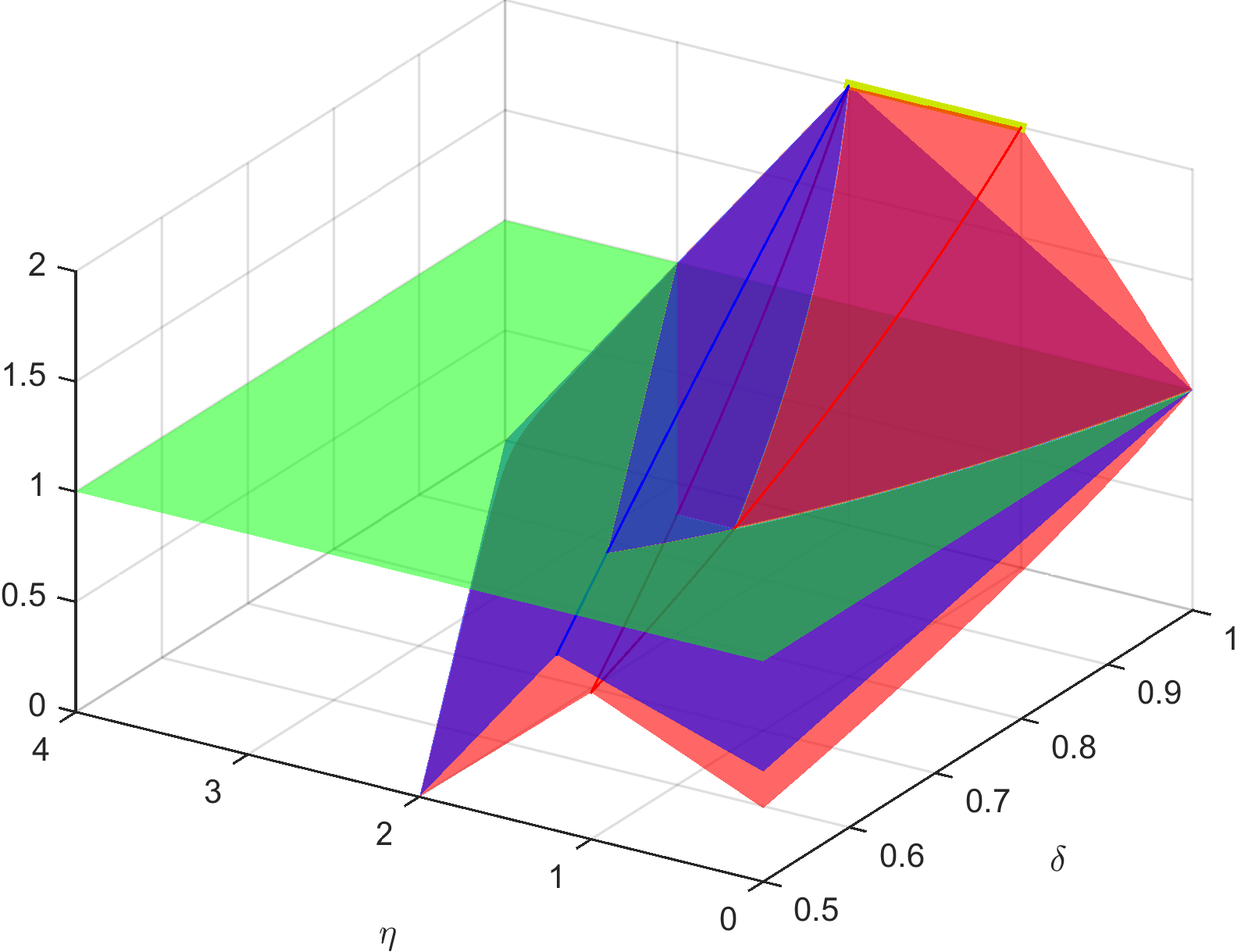
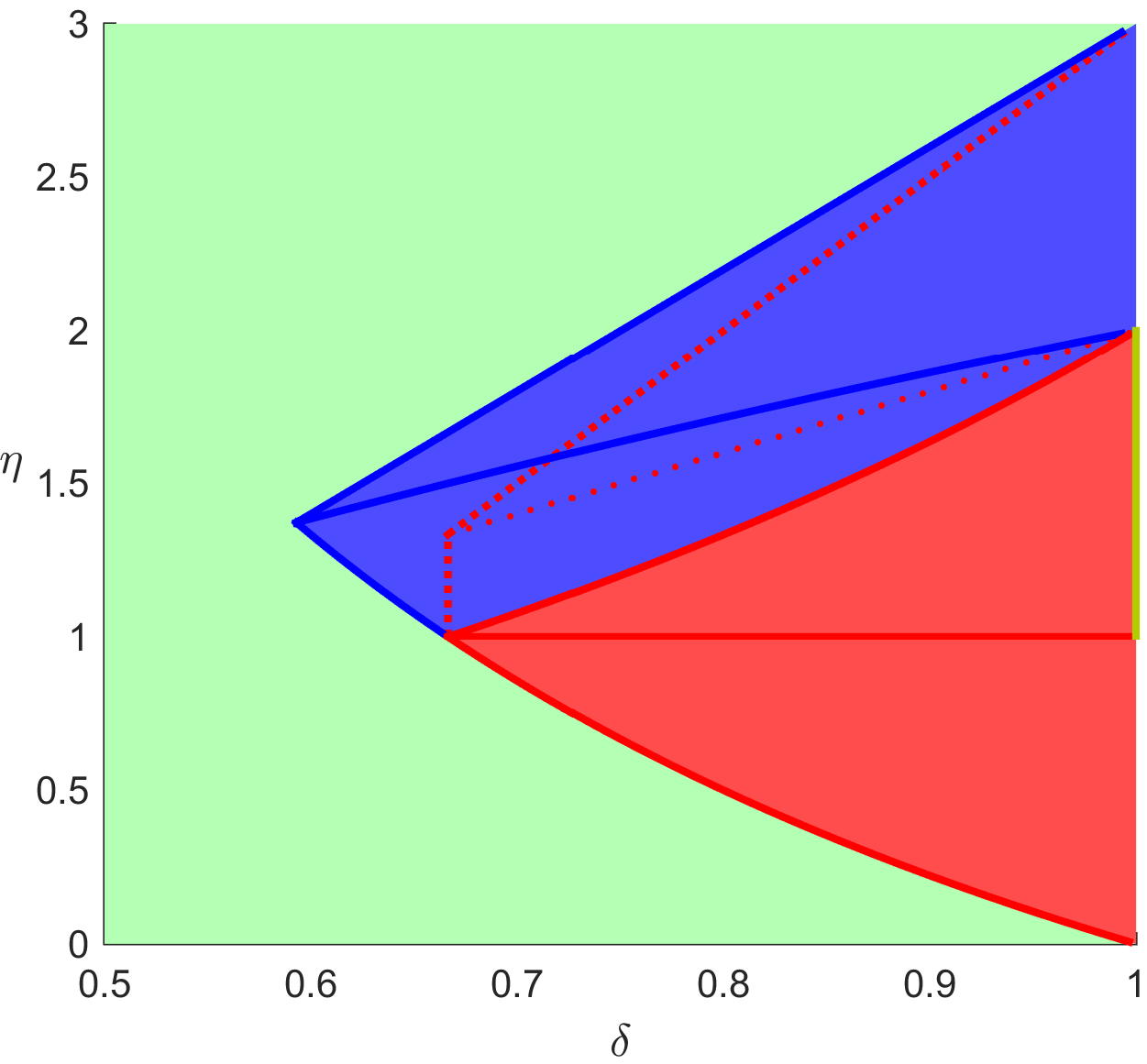
(ii) The values of and are maximised when and , respectively, in which case and , having then .
Remark 3
In light of Proposition 1, the extent of the results that can be derived from Propositions 3 and 4 is rather reduced when is an isolated solution and is not full rank, since it imposes . Note that the function given as an example in (Guo2015, , Section 5) is Hölder metrically subregular of order , but is not Lipschitz continuous around any zero of the function, so it does not satisfy (A2) for (and, therefore, it does not satisfy (Guo2015, , Assumption 4.1) either). However, with the additional assumption that the Łojasiewicz gradient inequality (9) holds, we will obtain local convergence for all (see Theorem 3.2).
Next, we proceed to derive the main result of this section from Propositions 3 and 4, where we provide a region from which the parameter must be chosen so that superlinear convergence is guaranteed. Recall that a sequence is said to converge superlinearly to with order if converges to and there exists such that for all sufficiently large.
Theorem 3.1
Assume that and . Then, there exists some such that, for every sequence generated by 1 with , one has that is superlinearly convergent to with order given by (19). Further, the sequence converges to a solution , and if , its rate of convergence is also superlinear with order . Moreover, if and , all the latter holds with order given by (22).
Proof
We assume that for all (otherwise, the statement trivially holds). Let , be defined as in Proposition 2 and , be defined as in the proof of Proposition 3. Since , we have that for all sufficiently large. As , we deduce that
| (26) |
Define
Note that , because and .
Pick any and let be an infinite sequence generated by 1. First, we will show by induction that . It follows from and (12) that
| (27) |
Let us assume now that for . Then, from Proposition 3 and the definition of , we have
which yields
| (28) |
The latter inequality, together with (12), (26) and (27), implies
which completes the induction. Thus, we have shown that for all , as claimed.
From Proposition 3, we obtain that is superlinearly convergent to . Further, it follows from (12) and (28) that
Denoting by , we have that is a Cauchy sequence. Then, for any , we have
| (29) |
which implies that is also a Cauchy sequence. Thus, the sequence converges to some . Since for all and converges to , we have .
Remark 4
Our results above generalise the results in Guo2015 ; ZhuLin16 , not only because in these works they assume to be Lipschitz continuous (i.e., ), but also because the parameter considered by these authors is equal to . Furthermore, in their convergence results, cf. (Guo2015, , Theorem 4.1 and Theorem 4.2) and (ZhuLin16, , Theorem 2.1 and Theorem 2.2), the authors assume and , respectively, which both entail , so we have slightly improved the lower bound on for the superlinear convergence in Theorem 3.1.
As a direct consequence of Theorem 3.1, whenever and , we can derive quadratic convergence of the sequence generated by 1.
Corollary 1
Assume that and . Then, there exists such that for every sequence generated by 1 with , one has that is superlinearly convergent to with order
Moreover, the sequence converges superlinearly with order to a solution . Therefore, when and , the sequence is quadratically convergent to , and the sequence converges quadratically to a solution .
Remark 5
Example 3 (Example 2 revisited)
Let and be the functions defined in Example 2. The function does not satisfy the assumptions of Theorem 3.1, since . On the other hand, if and the starting point is chosen sufficiently close to , Theorem 3.1 proves for the function the superlinear convergence of the sequence generated by 1 to with order
Note that, since the solution is locally unique, the additional assumption is not needed. The order of convergence is thus maximised when .
The question of whether the sequence converges to when does not satisfy the requirements commented in Remark 2(i) remains open. However, with the additional assumption that satisfies the Łojasiewicz gradient inequality (which holds for real analytic functions), we can prove that the sequences and converge to for all as long as the parameter is sufficiently small, and we can also provide a rate of convergence that depends on the exponent of the Łojasiewicz gradient inequality. This is the subject of the next subsection.
3.1 Convergence analysis under the Łojasiewicz gradient inequality
To prove our convergence result, we make use of the following two lemmas.
Lemma 1
Let be a nonnegative real sequence and let be some nonnegative constants. Suppose that and that the sequence satisfies
Then
-
(i)
if , the sequence converges to in a finite number of steps;
-
(ii)
if , the sequence converges linearly to with rate ;
-
(iii)
if , there exists such that
Proof
See (artacho_accelerating_2015, , Lemma 1).∎
Lemma 2
Proof
This result is a straightforward modification of (karas2015algebraic, , Theorem 2.5 and Lemma 2.3), using (2) instead of the Lipschitz continuity of .∎
In our second main result of this paper, under the additional assumption that the Łojasiewicz gradient inequality holds, we prove the convergence to of the sequences and .
Theorem 3.2
Suppose that satisfies the Łojasiewicz gradient inequality (9) with exponent . Let
| (30) |
Then, if , there exist some positive constants and such that, for every and every sequence generated by 1, one has and the two sequences and converge to . Moreover, the following holds:
-
(i)
if , the sequences and converge linearly to ;
-
(ii)
if , there exist some positive constants and such that, for all large ,
Proof
The proof has three key parts.
In the first part of the proof, we will set the values of and . Let and be such that (9) holds. Thus, one has
| (31) |
Let . Then, by Assumption (A1), there exists some positive constant such that
| (32) |
Since , it is possible to make smaller if needed to ensure, for all , that
| (33) |
For all , one has by the Lipschitz continuity of that
| (34) |
since . Let
Then, since and , we have .
In the second part of the proof, we will prove by induction that
| (35) | |||
| (36) |
for all . Pick any and let be the sequence generated by 1. It follows from Lemma 2 that
| (37) |
for all , where , since . Since , we have by (31), the definition of in (30) and (33) that
| (38) |
which implies
Therefore, from (37), we get
| (39) |
Observe that the convexity of the function with yields
| (40) |
for all . By combining (39) with (40), we deduce
| (41) |
Since , we have by (32) that . Further, by the Łojasiewicz gradient inequality (9), it holds
From the last inequality, together with (41), the first inequality in (38) and then (34), we obtain
which, in particular, proves (36) for . Hence,
Therefore, . Assume now that (35)–(36) holds for all . Since , by (33) and the same argumentation as in (38), we have
which implies
Therefore, by (37), we get
| (42) |
Combining the latter inequality with (40), we deduce
| (43) |
Further, since , from the Łojasiewicz gradient inequality (9) and (32), it holds
From the last inequality and (43), we deduce
which proves (36) for . Hence, by (34), we have
which proves (35) for . This completes the second part of the proof.
In the third part of the proof, we will finally show the assertions in the statement of the theorem. From the second part of the proof we know that for all . This, together with (32), implies that for all . Thus,
Therefore, by (42), we have
It follows from the Łojasiewicz gradient inequality (9) and the last inequality that
This implies that converges to . By applying Lemma 1 with , and , we conclude that the rate of convergence depends on as claimed in (i)-(ii). Finally, observe that converges to with the rate stated in (i)-(ii) thanks to the Hölder metric subregularity of the function .∎
Remark 6
Observe that every real analytic function satisfies the assumptions of Theorem 3.2, thanks to Fact 1 and the discussion after it in Section 2. Therefore, local sublinear convergence of 1 is guaranteed for all sufficiently small (i.e., whenever ). This is the best that we can get with these weak assumptions, as we show in the next example.
Example 4 (Example 2 revisited)
Let be the function considered in Example 2. The function does not satisfy the assumptions of Theorem 3.1, but it verifies the ones of Theorem 3.2. Indeed, it is straightforward to check that satisfies the Łojasiewicz gradient inequality (9) with exponent . Since , we can only guarantee the sublinear convergence of the sequence generated by 1 to when . In fact, this is the best convergence rate that we can get. Indeed, a direct computation gives us
| (44) |
On the one hand, when and , we have . Therefore, it follows from (44) and that
which means that is sublinearly convergent to . This coincides with what Theorem 3.2 asserts, since . On the other hand, when and , sublinear convergence is also obtained from (44), which is exactly what Theorem 3.2 guarantees for all .
4 Application to biochemical reaction networks
In this section, we introduce first a class of nonlinear equations arising in the study of biochemistry, cf. Fleming2012 . After that, we compare the performance of 1 with various Levenberg–Marquardt algorithms for finding steady states of nonlinear systems of biochemical networks on 20 different real data biological models.
4.1 Nonlinear systems in biochemical reaction networks
Consider a biochemical network with molecular species and reversible elementary reactions111An elementary reaction is a chemical reaction for which no intermediate molecular species need to be postulated in order to describe the chemical reaction on a molecular scale.. We define forward and reverse stoichiometric matrices, , respectively, where denotes the stoichiometry222Reaction stoichiometry is a quantitative relationship between the relative quantities of molecular species involved in a single chemical reaction. of the molecular species in the forward reaction and denotes the stoichiometry of the molecular species in the reverse reaction. We assume that every reaction conserves mass, that is, there exists at least one positive vector satisfying , cf. gevorgyan2008detection . The matrix represents net reaction stoichiometry and may be viewed as the incidence matrix of a directed hypergraph, see Klamt2009 . We assume that there are less molecular species than there are net reactions, that is . We assume the cardinality of each row of and is at least one, and the cardinality of each column of is at least two. The matrices and are sparse and the particular sparsity pattern depends on the particular biochemical network being modeled. Moreover, we also assume that , which is a requirement for kinetic consistency, cf. Fleming20161 .
Let denote a variable vector of molecular species concentrations. Assuming constant nonnegative elementary kinetic parameters , we assume elementary reaction kinetics for forward and reverse elementary reaction rates as and , respectively, where and denote the respective componentwise functions, see, e.g., artacho_accelerating_2015 ; Fleming20161 . Then, the deterministic dynamical equation for time evolution of molecular species concentration is given by
A vector is a steady state if and only if it satisfies
Note that a vector is a steady state of the biochemical system if and only if
here denotes the null space of . Therefore, the set of steady states is unchanged if we replace the matrix by a matrix with the same null space. Suppose that is the submatrix of whose rows are linearly independent, then If one replaces by and transforms (4.1) to logarithmic scale, by letting , , then the right-hand side of (4.1) is equal to the function
where stands for the horizontal concatenation operator.
Let denote a basis for the left null space of , which implies . We have . We say that the system satisfies moiety conservation if for any initial concentration , it holds
along the trajectory of (4.1), given an initial starting point . It is possible to compute such that each row corresponds to a structurally identifiable conserved moiety in a biochemical network, cf. Haraldsdttir2016 . The problem of finding the moiety conserved steady state of a biochemical reaction network is equivalent to solving the nonlinear equation (1) with
| (46) |
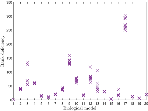
By replacing by we have improved the rank deficiency of , and thus the one of in (46). Nonetheless, as we demonstrate in Figure 5, is usually still far from being full rank at the solutions.
Let us show that is real analytic. Let and . Then we can write
where Since are nonnegative integers for all and , we conclude that the function is real analytic (see Proposition 2.2.2 and Proposition 2.2.8 in parks1992primer ). It follows from Remark 6 that satisfy the Łojasiewicz gradient inequality (with some unknown exponent ) and the mapping is Hölder metrically subregular around . Therefore, the assumptions of Theorem 3.2 are satisfied as long as is sufficiently small, and local sublinear convergence of 1 is guaranteed.
4.2 Computational experiments
In this subsection, we compare 1 with various Levenberg–Marquardt methods for solving the nonlinear system (1) with defined by (46) on 20 different biological models. These codes are available in the COBRA Toolbox v3 COBRA . In our implementation, all codes were written in MATLAB and runs were performed on Intel Core i7-4770 CPU 3.40GHz with 12GB RAM, under Windows 10 (64-bits). The algorithms were stopped whenever
is satisfied or the maximum number of iterations (say 10,000) is reached. On the basis of our experiments with the mapping (46), we set
| (47) |
The initial point is set to in all the experiments.
To illustrate the results, we use the Dolan and Moré performance profile Dolan2002 with the performance measures and , where and denote the total number of iterations and the running time. In this procedure, the performance of each algorithm is measured by the ratio of its computational outcome versus the best numerical outcome of all algorithms. This performance profile offers a tool to statistically compare the performance of algorithms. Let be a set of all algorithms and be a set of test problems. For each problem and algorithm , denotes the computational outcome with respect to the performance index, which is used in the definition of the performance ratio
| (48) |
If an algorithm fails to solve a problem , the procedure sets , where should be strictly larger than any performance ratio (48). Let be the number of problems in the experiment. For any factor , the overall performance of an algorithm is given by
Here, is the probability that a performance ratio of an algorithm is within a factor of the best possible ratio. The function is a distribution function for the performance ratio. In particular, gives the probability that an algorithm wins over all other considered algorithms, and gives the probability that algorithm solves all considered problems. Therefore, this performance profile can be considered as a measure of efficiency among all considered algorithms.
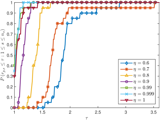
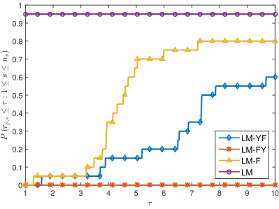
In our first experiment, we explore for which parameter the best performance of 1 is obtained. To this end, we apply seven versions of 1 associated to each of the parameters to the nonlinear system (46) defined by 20 biological models. The results of this comparison are summarised in Table 1 and Figure 2, from where it can be observed that 1 with outperforms the other values of the parameters. It is also apparent that smaller values of are less efficient, although 1 successfully found a solution for every model and every value of that was tested. It is important to recall here that local convergence is only guaranteed by Theorem 3.2 for sufficiently small values of , since the value of is unknown. Also, note that the local convergence for the value is not covered by Theorem 3.2 for our choice of the parameters, because it requires , since in (47).
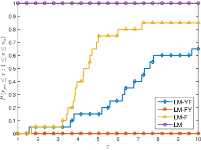
We now set and compare 1 with parameters (47) with the following Levenberg–Marquardt methods:
-
LM-YF: with , given by Yamashita and Fukushima alefeld_rate_2001 ;
-
LM-FY: with , given by Fan and Yuan fan_quadratic_2005 ;
-
LM-F: with , given by Fischer fischer2002local .
It is clear that all of these three methods are special cases of 1 by selecting suitable parameters , , and . The results of our experiments are summarised in Table 2 and Figure 3. In Figures 3(a) and 3(b), we see that 1 is clearly always the winner, both for the number of iterations and the running time. Moreover, LM-F outperforms both LM-YF and LM-FY. In fact, LM-FY was not able to solve any of the considered problems within the 10,000 iterations.
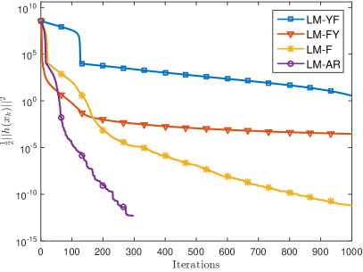
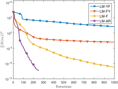
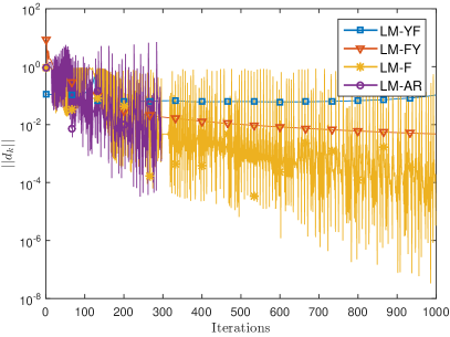
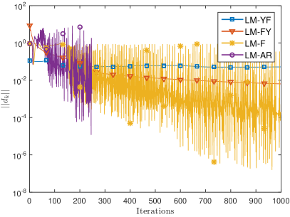
In order to see the evolution of the merit function, we illustrate its value with respect to the number of iterations in Figure 4 for the mapping (46) with the biological models iAF692 and iNJ661. We limit the maximum number of iterations to 1,000. Clearly, 1 attains the best results, followed by LM-F. Both methods seem to be more suited to biological problems than LM-YF and LM-FY. We also show in Figure 4 the evolution of the value of the step size . Both 1 and LM-F show a rippling behaviour, while the value of is nearly constant along the 1,000 iterations for LM-YF and LM-FY. Probably, this rippling behaviour is letting the first two methods escape from a flat valley of the merit function, while the two last methods get trapped there. Observe also that, by Lemma 2, one has that for LM-YF and for LM-FY, while this upper bound can be larger for both 1 and LM-F.
In our last experiment, we find solutions of the nonlinear system (1) with 1 using random starting points for each of the biological models and compute the rank of at each of these solutions. The results are shown in Figure 5, where we plot the rank deficiency of at each of the solutions. For all the models, except for the Ecoli_core, we observe that at the solutions found is far from being full rank. For the Ecoli_core, although had full rank at every solution found, the smallest eigenvalue at these solutions had a value around , making also this problem ill-conditioned. This explains the difficulties that most of the algorithms had for solving the nonlinear system (1) with defined by (46). Therefore, since we are dealing with a difficult problem, it is more meritorious the successfulness of 1 with parameters (47) for finding a solution of each of the models in less than 400 iterations (in less than one minute), as shown in Table 2.
5 Conclusion and further research
We have presented an adaptive Levenberg–Marquardt method for solving systems of nonlinear equations with possible non-isolated solutions. We have analysed its local convergence under Hölder metric subregularity of the underlying function and Hölder continuity of its gradient. We have further analysed the local convergence under the additional assumption that the Łojasiewicz gradient inequality holds. These properties hold in many applied problems, as they are satisfied by any real analytic function. One of these applications is computing a solution to a system of nonlinear equations arising in biochemical reaction networks, a problem which is usually ill-conditioned. We showed that such systems satisfy both the Hölder metric subregularity and the Łojasiewicz gradient inequality assumptions. In our numerical experiments, we clearly obtained a superior performance of our regularisation parameter, compared to existing Levenberg–Marquardt methods, for 20 different biological networks.
Several extensions to the present study are possible, the most important of which would be to develop a globally convergent version of the proposed Levenberg–Marquardt method. One approach, which is currently being investigated, would be to combine the scheme with an Armijo-type line search and a trust-region technique. This will be reported in a separate article AFV19 . It would also be interesting to analyse a regularisation parameter where the value of is updated at each iteration. The analysis of the convergence with such a parameter would be much more involved, so we leave this for future work.
Acknowledgements
We would like to thank Mikhail Solodov for suggesting the use of Levenberg–Marquardt methods for solving the system of nonlinear equations arising in biochemical reaction networks. Thanks also go to Michael Saunders for his useful comments on the first version of this manuscript. We are grateful to two anonymous reviewers for their constructive comments, which helped us improving the paper.
Appendix
| Model | |||||||||||||||||
|---|---|---|---|---|---|---|---|---|---|---|---|---|---|---|---|---|---|
| 1. Ecoli_core | 72 | 73 | 61 | 210 | 0.10 | 191 | 0.08 | 179 | 0.07 | 159 | 0.06 | 136 | 0.06 | 138 | 0.04 | 139 | 0.09 |
| 2. iAF692 | 462 | 493 | 430 | 492 | 6.89 | 421 | 5.70 | 328 | 4.54 | 291 | 3.98 | 274 | 3.72 | 256 | 3.44 | 253 | 3.42 |
| 3. iAF1260 | 1520 | 1931 | 1456 | 473 | 98.75 | 410 | 83.41 | 357 | 74.05 | 334 | 68.65 | 257 | 53.69 | 271 | 57.05 | 268 | 54.88 |
| 4. iBsu1103 | 993 | 1167 | 956 | 421 | 34.34 | 356 | 28.46 | 313 | 25.14 | 254 | 20.34 | 232 | 18.38 | 218 | 17.13 | 226 | 18.04 |
| 5. iCB925 | 415 | 558 | 386 | 467 | 6.41 | 477 | 6.47 | 332 | 4.55 | 296 | 4.30 | 318 | 4.39 | 248 | 3.33 | 350 | 4.71 |
| 6. iIT341 | 424 | 428 | 392 | 388 | 4.33 | 333 | 3.48 | 253 | 2.68 | 226 | 2.29 | 207 | 2.13 | 226 | 2.34 | 212 | 2.19 |
| 7. iJN678 | 641 | 669 | 589 | 362 | 9.63 | 356 | 8.99 | 307 | 7.76 | 258 | 6.72 | 220 | 5.76 | 231 | 5.89 | 218 | 5.60 |
| 8. iJN746 | 727 | 795 | 700 | 470 | 17.05 | 376 | 13.29 | 301 | 10.66 | 255 | 8.93 | 256 | 9.26 | 231 | 8.17 | 251 | 9.10 |
| 9. iJO1366 | 1654 | 2102 | 1582 | 417 | 107.37 | 372 | 95.21 | 314 | 79.85 | 273 | 70.62 | 225 | 57.36 | 219 | 55.65 | 244 | 62.37 |
| 10. iJR904 | 597 | 757 | 564 | 441 | 11.99 | 420 | 11.15 | 346 | 8.80 | 279 | 7.26 | 245 | 6.34 | 249 | 6.39 | 253 | 6.98 |
| 11. iMB745 | 525 | 598 | 490 | 363 | 7.13 | 346 | 6.48 | 298 | 5.55 | 211 | 3.85 | 204 | 3.74 | 218 | 4.02 | 199 | 3.66 |
| 12. iNJ661 | 651 | 764 | 604 | 549 | 16.21 | 436 | 12.68 | 366 | 11.01 | 283 | 8.30 | 222 | 6.45 | 257 | 7.53 | 254 | 7.57 |
| 13. iRsp1095 | 966 | 1042 | 921 | 655 | 54.48 | 1057 | 92.98 | 374 | 28.20 | 333 | 25.03 | 301 | 21.89 | 301 | 22.63 | 336 | 25.52 |
| 14. iSB619 | 462 | 508 | 435 | 373 | 5.13 | 344 | 4.60 | 295 | 3.95 | 243 | 3.24 | 203 | 2.73 | 221 | 2.97 | 215 | 2.85 |
| 15. iTH366 | 583 | 606 | 529 | 349 | 7.27 | 338 | 6.91 | 279 | 5.67 | 219 | 4.46 | 212 | 4.33 | 204 | 4.16 | 207 | 4.21 |
| 16. iTZ479_v2 | 435 | 476 | 415 | 375 | 4.54 | 344 | 4.00 | 297 | 3.45 | 228 | 2.68 | 204 | 2.39 | 214 | 2.48 | 227 | 2.63 |
| 17. iYL1228 | 1350 | 1695 | 1280 | 846 | 136.52 | 550 | 87.18 | 387 | 60.96 | 326 | 51.24 | 294 | 46.28 | 318 | 49.99 | 293 | 46.18 |
| 18. L_lactis_MG1363 | 483 | 491 | 429 | 463 | 6.54 | 427 | 5.89 | 351 | 4.80 | 314 | 4.36 | 279 | 3.85 | 242 | 3.35 | 282 | 3.87 |
| 19. Sc_thermophilis_rBioNet | 348 | 365 | 320 | 413 | 2.85 | 377 | 2.57 | 344 | 2.31 | 291 | 1.97 | 252 | 1.66 | 256 | 1.69 | 241 | 1.63 |
| 20. T_Maritima | 434 | 470 | 414 | 407 | 4.83 | 318 | 3.72 | 281 | 3.26 | 233 | 2.70 | 231 | 2.65 | 215 | 2.49 | 212 | 2.44 |
| Average | 447 | 27.12 | 412 | 24.16 | 315 | 17.36 | 265 | 15.05 | 239 | 12.85 | 237 | 13.04 | 244 | 13.4 | |||
| Model | LM-YF | LM-FY | LM-F | 1 | |||||||
|---|---|---|---|---|---|---|---|---|---|---|---|
| 1. Ecoli_core | 72 | 73 | 61 | 238 | 0.10 | 10000 | 4.06 | 257 | 0.08 | 153 | 0.06 |
| 2. iAF692 | 462 | 493 | 430 | 1685 | 23.43 | 10000 | 135.63 | 1358 | 18.15 | 271 | 3.61 |
| 3. iAF1260 | 1520 | 1931 | 1456 | 8233 | 1726.92 | 10000 | 2066.38 | 2036 | 413.04 | 283 | 57.27 |
| 4. iBsu1103 | 993 | 1167 | 956 | 2396 | 187.24 | 10000 | 780.72 | 761 | 59.39 | 193 | 15.09 |
| 5. iCB925 | 415 | 558 | 386 | 1005 | 14.15 | 10000 | 131.01 | 10000 | 131.28 | 278 | 3.82 |
| 6. iIT341 | 424 | 428 | 392 | 1407 | 14.77 | 10000 | 103.09 | 944 | 9.71 | 222 | 2.26 |
| 7. iJN678 | 641 | 669 | 589 | 2218 | 56.33 | 10000 | 253.58 | 1043 | 26.34 | 229 | 5.82 |
| 8. iJN746 | 727 | 795 | 700 | 3107 | 108.72 | 10000 | 349.43 | 1069 | 37.18 | 217 | 7.53 |
| 9. iJO1366 | 1654 | 2102 | 1582 | 7716 | 1946.48 | 10000 | 2524.01 | 1066 | 268.38 | 232 | 58.33 |
| 10. iJR904 | 597 | 757 | 564 | 2789 | 72.26 | 10000 | 258.50 | 1231 | 31.74 | 262 | 6.75 |
| 11. iMB745 | 525 | 598 | 490 | 790 | 14.60 | 10000 | 181.40 | 1247 | 22.50 | 208 | 3.76 |
| 12. iNJ661 | 651 | 764 | 604 | 2635 | 76.62 | 10000 | 290.56 | 1357 | 39.45 | 360 | 10.44 |
| 13. iRsp1095 | 966 | 1042 | 921 | 3832 | 266.87 | 10000 | 694.21 | 10000 | 696.93 | 235 | 16.38 |
| 14. iSB619 | 462 | 508 | 435 | 1581 | 21.42 | 10000 | 133.94 | 814 | 10.82 | 233 | 3.12 |
| 15. iTH366 | 583 | 606 | 529 | 1641 | 33.78 | 10000 | 205.34 | 817 | 16.79 | 211 | 4.30 |
| 16. iTZ479_v2 | 435 | 476 | 415 | 1148 | 13.57 | 10000 | 117.46 | 713 | 8.34 | 221 | 2.61 |
| 17. iYL1228 | 1350 | 1695 | 1280 | 6070 | 956.92 | 10000 | 1565.75 | 10000 | 1567.47 | 272 | 42.94 |
| 18. L_lactis_MG1363 | 483 | 491 | 429 | 2180 | 30.17 | 10000 | 137.99 | 1231 | 17.06 | 287 | 4.10 |
| 19. Sc_thermophilis_rBioNet | 348 | 365 | 320 | 1753 | 11.85 | 10000 | 68.54 | 935 | 6.33 | 244 | 1.61 |
| 20. T_Maritima | 434 | 470 | 414 | 1169 | 14.33 | 10000 | 118.65 | 717 | 8.31 | 209 | 2.42 |
| Average of successful | 2680 | 279.53 | — | — | 1035 | 58.45 | 241 | 12.61 | |||
References
- (1) M. Ahookhosh, R.M.T. Fleming, P.T. Vuong: Finding zeros of Hölder metrically subregular mappings via globally convergent Levenberg–Marquardt methods, arXiv: 1812.00818.
- (2) Aragón Artacho, F.J., Fleming, R.: Globally convergent algorithms for finding zeros of duplomonotone mappings. Optim. Lett. 9(3), 569–584 (2015).
- (3) Aragón Artacho, F.J., Fleming, R., Vuong, P.T.: Accelerating the DC algorithm for smooth functions. Math. Program. 169B(1), 95–118 (2018).
- (4) Attouch, H., Bolte, J.: On the convergence of the proximal algorithm for nonsmooth functions involving analytic features. Math. Program. 116(1-2), 5–16 (2009).
- (5) Attouch, H., Bolte, J., Svaiter, B.F.: Convergence of descent methods for semi-algebraic and tame problems: proximal algorithms, forward-backward splitting, and regularized Gauss-Seidel methods. Math.Program. 137A(1-2), 91–129 (2013).
- (6) Behling, R., Iusem, A.: The effect of calmness on the solution set of systems of nonlinear equations. Math. Program. 137A(1-2), 155–165 (2013).
- (7) Bellavia, S., Cartis, C., Gould, N., Morini, B., Toint, P.L.: Convergence of a regularized Euclidean residual algorithm for nonlinear least squares. SIAM J. Numer. Anal. 48(1), 1–29 (2010).
- (8) Bellavia, S., Morini, B.: Strong local convergence properties of adaptive regularized methods for nonlinear least squares. IMA J. Numer. Anal. 35(2), 947–968 (2015).
- (9) Bolte, J., Daniilidis, A., Lewis, A.: The Łojasiewicz inequality for nonsmooth subanalytic functions with applications to subgradient dynamical systems. SIAM J. Optimiz. 17(4), 1205–1223 (2007).
- (10) Bolte, J., Daniilidis, A., Ley, O., Mazet, L.: Characterizations of Lojasiewicz inequalities: subgradient flows, talweg, convexity. Trans. Amer. Math. Soc. 362(6), 3319–3363 (2010).
- (11) Cibulka, R., Dontchev, A.L., Kruger, A.Y.: Strong metric subregularity of mappings in variational analysis and optimization. J. Math. Anal. Appl. 457(2), 1247–1282 (2018).
- (12) Dolan, E.D., Moré, J.J.: Benchmarking optimization software with performance profiles. Math. Program. 91B(2), 201–213 (2002).
- (13) Dontchev, A.L., Rockafellar, R.T.: Implicit Functions and Solution Mappings, 2. ed. edn. Springer Series in Operations Research and Financial Engineering. Springer, New York, NY [u.a.] (2014).
- (14) Eilenberger, G.: Solitons: Mathematical methods for physicists. Springer-Verlag (1983).
- (15) Fan, J.: Convergence rate of the trust region method for nonlinear equations under local error bound condition. Comput. Optim. Appl. 34(2), 215–227 (2006).
- (16) Fan, J.: The modified Levenberg–Marquardt method for nonlinear equations with cubic convergence. Math. Comput. 81(277), 447–466 (2012).
- (17) Fan, J., Pan, J.: A note on the Levenberg–Marquardt parameter. Appl. Math. Comput. 207, 351–359 (2009).
- (18) Fan, J., Yuan, Y.: On the quadratic convergence of the Levenberg–Marquardt method without nonsingularity assumption. Computing 74(1), 23–39 (2005).
- (19) Fischer, A.: Local behavior of an iterative framework for generalized equations with nonisolated solutions. Math. Program. 94B(1), 91–124 (2002).
- (20) Fischer, A., Herrich, M., Izmailov, A.F., Solodov, M.V.: A globally convergent LP–Newton method. SIAM J. Optim. 26(4), 2012–2033 (2015).
- (21) Fleming, R., Thiele, I.: Mass conserved elementary kinetics is sufficient for the existence of a non-equilibrium steady state concentration. J. Theoret. Biol. 314, 173–181 (2012).
- (22) Fleming, R.M., Vlassis, N., Thiele, I., Saunders, M.A.: Conditions for duality between fluxes and concentrations in biochemical networks. J. Theoret. Biol. 409, 1–10 (2016).
- (23) Gevorgyan, A., Poolman, M., Fell, D.: Detection of stoichiometric inconsistencies in biomolecular models. Bioinformatics 24(19), 2245–2251 (2008).
- (24) Guo, L., Lin, G.H., Ye, J.J.: Solving mathematical programs with equilibrium constraints. J. Optim. Theory Appl. 166(1), 234–256 (2015).
- (25) Gwoździewicz, J.: The Łojasiewicz exponent of an analytic function at an isolated zero. Comment. Math. Helv. 74(3), 364–375 (1999).
- (26) Haraldsdóttir, H.S., Fleming, R.M.: Identification of conserved moieties in metabolic networks by graph theoretical analysis of atom transition networks. PLoS Comput. Biol. 12(11), e1004,999 (2016).
- (27) Hasegawa, A.: Plasma Instabilities and Nonlinear Effects. Springer Berlin Heidelberg, Berlin, Heidelberg (1975).
- (28) Heirendt, L., et al.: Creation and analysis of biochemical constraint-based models: the COBRA Toolbox v3.0. To appear in Nat. Protoc., DOI: 10.1038/s41596-018-0098-2.
- (29) Hoffman, A.: On approximate solutions of systems of linear inequalities. J. Res. Nat. Bur. Standards 49, 263–265 (1952).
- (30) Izmailov, A.F., Solodov, M.V.: Error bounds for 2-regular mappings with Lipschitzian derivatives and their applications. Math. Program. 89B(3), 413–435 (2001).
- (31) Izmailov, A.F., Solodov, M.V.: The theory of 2-regularity for mappings with Lipschitzian derivatives and its applications to optimality conditions. Math. Oper. Res. 27(3), 614–635 (2002).
- (32) Izmailov, A.F., Solodov, M.V.: Newton-Type Methods for Optimization and Variational Problems. Springer (2014).
- (33) Kanzow, C., Yamashita, N., Fukushima, M.: Levenberg–Marquardt methods with strong local convergence properties for solving nonlinear equations with convex constraints. J. Comput. Appl. Math. 172(2), 375–397 (2004).
- (34) Karas, E.W., Santos, S.A., Svaiter, B.F.: Algebraic rules for computing the regularization parameter of the Levenberg–Marquardt method. Comput. Optim. Appl. 65(3), 723–751 (2016).
- (35) Kelley, C.: Iterative Methods for Optimization. Frontiers Appl. Math. 18, SIAM, Philadelphia (1999)
- (36) Klamt, S., Haus, U.U., Theis, F.: Hypergraphs and cellular networks. PLoS Comput Biol 5(5), e1000,385 (2009).
- (37) Kruger, A.: Error bounds and Hölder metric subregularity. Set-Valued Var. Anal.23(4), 705–736 (2015).
- (38) Kurdyka, K., Spodzieja, S.: Separation of real algebraic sets and the Łojasiewicz exponent. Proc. Amer. Math. Soc. 142(9), 3089–3102 (2014).
- (39) Li, G., Mordukhovich, B.: Hölder metric subregularity with applications to proximal point method. SIAM J. Optim. 22(4), 1655–1684 (2012).
- (40) Lojasiewicz, S.: Ensembles semi-analytiques. Université de Gracovie (1965)
- (41) Ma, C., Jiang, L.: Some research on Levenberg–Marquardt method for the nonlinear equations. Appl. Math. Comput. 184, 1032–1040 (2007).
- (42) Mordukhovich, B.S.: Variational Analysis and Generalized Differentiation I. Springer, Berlin (2006).
- (43) Mordukhovich, B.S., Ouyang, W.: Higher-order metric subregularity and its applications. J. Global Optim. 63(4), 777–795 (2015).
- (44) Moré, J., Garbow, B., Hillstrom, K.: Testing unconstrained optimization software. ACM Trans. Math. Software 7(1), 17–41 (1981).
- (45) Ngai, H.V.: Global error bounds for systems of convex polynomials over polyhedral constraints. SIAM J. on Optim. 25(1), 521–539 (2015).
- (46) Nocedal, J., Wright, S.: Numerical Optimization. Springer, New York (2006).
- (47) Ortega, J., Rheinboldt, W.: Iterative Solution of Nonlinear Equations in Several Variables. Society for Industrial and Applied Mathematics (2000).
- (48) Pang, J.: Error bounds in mathematical programming. Math. Program. 79B(1–3), 299–332 (1997).
- (49) Parks, H., Krantz, S.: A Primer of Real Analytic Functions. Birkhäuser Verlag (1992).
- (50) Vui, H.: Global Hölderian error bound for nondegenerate polynomials. SIAM J. Optim. 23(2), 917–933 (2013).
- (51) Whitham, G.B.: Linear and Nonlinear Waves. Wiley, New York (1974).
- (52) Yamashita, N., Fukushima, M.: On the rate of convergence of the Levenberg–Marquardt method. In: G. Alefeld, X. Chen (eds.) Topics in Numerical Analysis, vol. 15, pp. 239–249. Springer Vienna, Vienna (2001).
- (53) Yuan, Y.: Recent advances in trust region algorithms. Math. Program. 151B(1), 249–281 (2015).
- (54) Zhu, X., Lin, G.H.: Improved convergence results for a modified Levenberg–Marquardt method for nonlinear equations and applications in MPCC. Optim. Methods Softw. 31(4), 791–804 (2016).