Dance Dance Convolution

Abstract

Dance Dance Revolution (DDR) is a popular rhythm-based video game. Players perform steps on a dance platform in synchronization with music as directed by on-screen step charts. While many step charts are available in standardized packs, players may grow tired of existing charts, or wish to dance to a song for which no chart exists. We introduce the task of learning to choreograph. Given a raw audio track, the goal is to produce a new step chart. This task decomposes naturally into two subtasks: deciding when to place steps and deciding which steps to select. For the step placement task, we combine recurrent and convolutional neural networks to ingest spectrograms of low-level audio features to predict steps, conditioned on chart difficulty. For step selection, we present a conditional LSTM generative model that substantially outperforms $n$-gram and fixed-window approaches.

1 Introduction

Figure 1: Proposed learning to choreograph pipeline for four seconds of the song Knife Party feat. Mistajam - Sleaze. The pipeline ingests audio features (Bottom) and produces a playable DDR choreography (Top) corresponding to the audio.

Dance Dance Revolution (DDR) is a rhythm-based video game with millions of players worldwide (Hoysniemi, 2006). Players perform steps atop a dance platform, following prompts from an on-screen step chart to step on the platform’s buttons at specific, musically salient points in time. A player’s score depends upon both hitting the correct buttons and hitting them at the correct time. Step charts vary in difficulty with harder charts containing more steps and more complex sequences. The dance pad contains up, down, left, and right arrows, each of which can be in one of four states: on, off, hold, or release. Because the four arrows can be activated or released independently, there are $256$ possible step combinations at any instant.

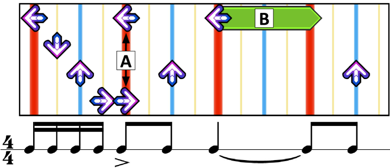
Step charts exhibit rich structure and complex semantics to ensure that step sequences are both challenging and enjoyable. Charts tend to mirror musical structure: particular sequences of steps correspond to different motifs (Figure 2), and entire passages may reappear as sections of the song are repeated. Moreover, chart authors strive to avoid patterns that would compel a player to face away from the screen.

The DDR community uses simulators, such as the open-source StepMania, that allow fans to create and play their own charts. A number of prolific authors produce and disseminate packs of charts, bundling metadata with relevant recordings. Typically, for each song, packs contain one chart for each of five difficulty levels.

Despite the game’s popularity, players have some reasonable complaints: For one, packs are limited to songs with favorable licenses, meaning players may be unable to dance to their favorite songs. Even when charts are available, players may tire of repeatedly performing the same charts. Although players can produce their own charts, the process is painstaking and requires significant expertise.

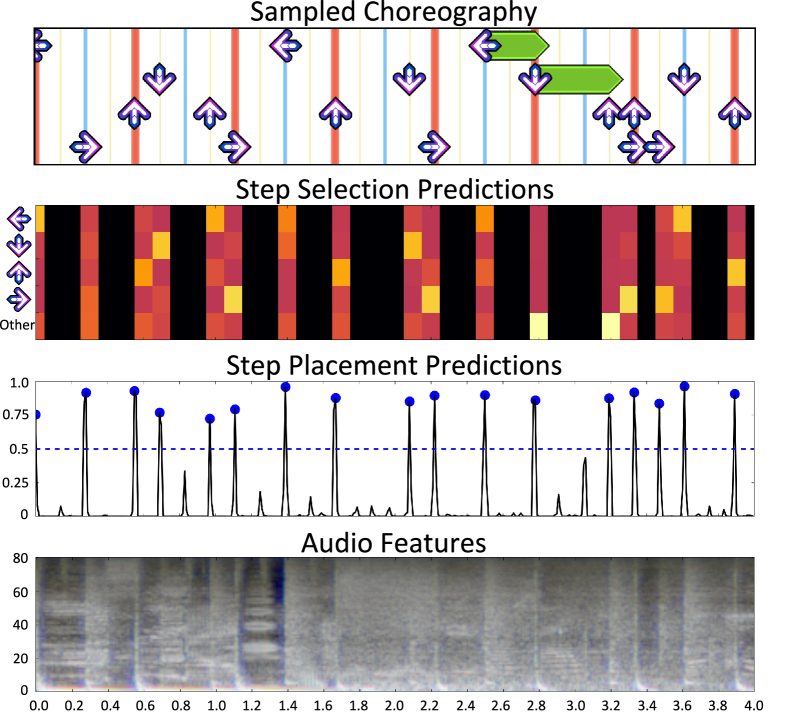
In this paper, we seek to automate the process of step chart generation so that players can dance to a wider variety of charts on any song of their choosing. We introduce the task of learning to choreograph, in which we learn to generate step charts from raw audio. Although this task has previously been approached via ad-hoc methods, we are the first to cast it as a learning task in which we seek to mimic the semantics of human-generated charts. We break the problem into two subtasks: First, step placement consists of identifying a set of timestamps in the song at which to place steps. This process can be conditioned on a player-specified difficulty level. Second, step selection consists of choosing which steps to place at each timestamp. Running these two steps in sequence yields a playable step chart. This process is depicted in Figure 1.

Figure 2: A four-beat measure of a typical chart and its rhythm depicted in musical notation. Red: quarter notes, Blue: eighth notes, Yellow: sixteenth notes, (A): jump step, (B): freeze step

Progress on learning to choreograph may also lead to advances in music information retrieval (MIR). Our step placement task, for example, closely resembles onset detection, a well-studied MIR problem. The goal of onset detection is to identify the times of all musically salient events, such as melody notes or drum strikes. While not every onset in our data corresponds to a DDR step, every DDR step corresponds to an onset. In addition to marking steps, DDR packs specify a metronome click track for each song. For songs with changing tempos, the exact location of each change and the new tempo are annotated. This click data could help to spur algorithmic innovation for beat tracking and tempo detection.

Unfortunately, MIR research is stymied by the difficulty of accessing large, well-annotated datasets. Songs are often subject to copyright issues, and thus must be gathered by each researcher independently. Collating audio with separately-distributed metadata is nontrivial and error-prone owing to the multiple available versions of many songs. Researchers often must manually align their version of a song to the metadata. In contrast, our dataset is publicly available, standardized and contains meticulously-annotated labels as well as the relevant recordings.

We believe that DDR charts represent an abundant and under-recognized source of annotated data for MIR research. StepMania Online, a popular repository of DDR data, distributes over $350\mathit{Gb}$ of packs with annotations for more than $100\mathit{k}$ songs. In addition to introducing a novel task and methodology, we contribute two large public datasets, which we consider to be of notably high quality and consistency. Each dataset is a collection of recordings and step charts. One contains charts by a single author and the other by multiple authors.

For both prediction stages of learning to choreograph, we demonstrate the superior performance of neural networks over strong alternatives. Our best model for step placement jointly learns a convolutional neural network (CNN) representation and a recurrent neural network (RNN), which integrates information across consecutive time slices. This method outperforms CNNs alone, multilayer perceptrons (MLPs), and linear models.

Our best-performing system for step selection consists of a conditional LSTM generative model. As auxiliary information, the model takes beat phase, a number representing the fraction of a beat at which a step occurs. Additionally, the best models receive the time difference (measured in beats) since the last and until the next step. This model selects steps that are more consistent with expert authors than the best $n$-gram and fixed-window models, as measured by perplexity and per-token accuracy.

1.1 Contributions

In short, our paper offers the following contributions:

• We define learning to choreograph, a new task with real-world usefulness and strong connections to fundamental problems in MIR.

• We introduce two large, curated datasets for benchmarking DDR choreography algorithms. They represent an under-recognized source of music annotations.

• We introduce an effective pipeline for learning to choreograph with deep neural networks.

2 Data

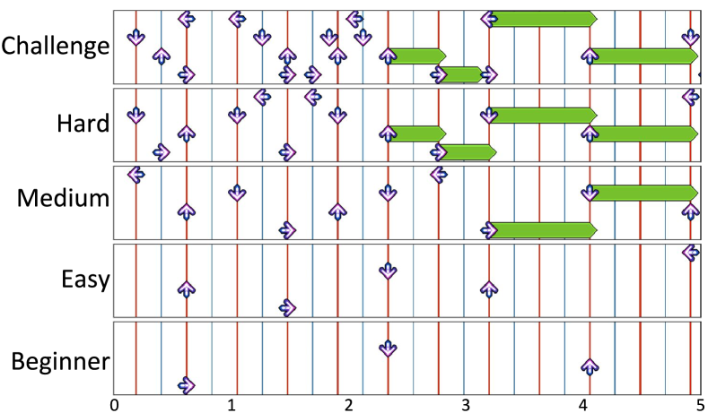
Basic statistics of our two datasets are shown in Table 1. The first dataset contains $90$ songs choreographed by a single prolific author who works under the name Fraxtil. This dataset contains five charts per song corresponding to increasing difficulty levels. We find that while these charts overlap significantly, the lower difficulty charts are not strict subsets of the higher difficulty charts (Figure 3). The second dataset is a larger, multi-author collection called In The Groove (ITG); this dataset contains $133$ songs with one chart per difficulty, except for $13$ songs that lack charts for the highest difficulty. Both datasets contain electronic music with constant tempo and a strong beat, characteristic of music favored by the DDR community.

Figure 3: Five seconds of choreography by difficulty level for the song KOAN Sound - The Edge from the Fraxtil training set.

Table 1: Dataset statistics

Dataset	Fraxtil	ITG
Num authors	1	8
Num packs	3	2
Num songs	90 (3.1 hrs)	133 (3.9 hrs)
Num charts	450 (15.3 hrs)	652 (19.0 hrs)
Steps/sec	3.135	2.584
Vocab size	81	88

Note that while the total number of songs is relatively small, when considering all charts across all songs the datasets contain around 35 hours of annotations and 350,000 steps. The two datasets have similar vocabulary sizes ($81$ and $88$ distinct step combinations, respectively). Around $84\%$ of the steps in both datasets consist of a single, instantaneous arrow.

Step charts contain several invariances, for example interchanging all instances of left and right results in an equally plausible sequence of steps. To augment the amount of data available for training, we generate four instances of each chart, by mirroring left/right, up/down (or both). Doing so considerably improves performance in practice.

In addition to encoded audio, packs consist of metadata including a song’s title, artist, a list of time-stamped tempo changes, and a time offset to align the recording to the tempos. They also contain information such as the chart difficulties and the name of the choreographer. Finally, the metadata contains a full list of steps, marking the measure and beat of each. To make this data easier to work with, we convert it to a canonical form consisting of (beat, time, step) tuples.

Figure 4: Number of steps per rhythmic subdivision by difficulty in the Fraxtil dataset.

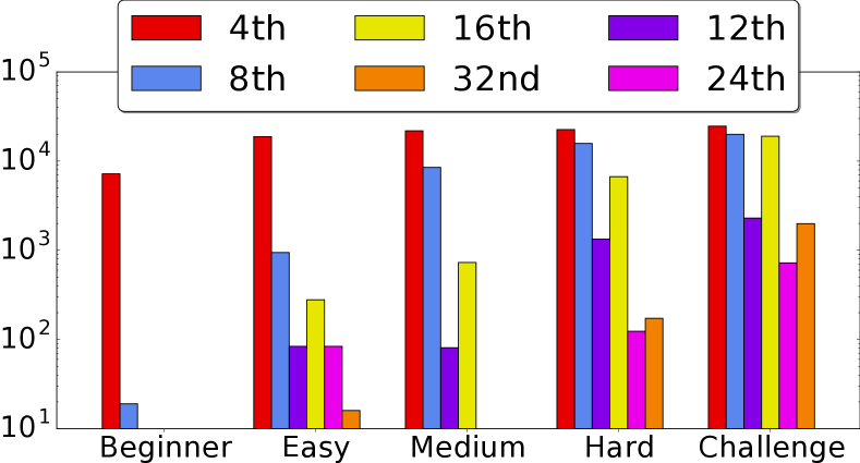
The charts in both datasets echo high-level rhythmic structure in the music. An increase in difficulty corresponds to increasing propensity for steps to appear at finer rhythmic subdivisions. Beginner charts tend to contain only quarter notes and eighth notes. Higher-difficulty charts reflect more complex rhythmic details in the music, featuring higher densities of eighth and sixteenth note steps (8th, 16th) as well as triplet patterns (12th, 24th) (Figure 4).

3 Problem Definition

A step can occur in up to $192$ different locations (subdivisions) within each measure. However, measures contain roughly 6 steps on average. This level of sparsity makes it difficult to uncover patterns across long sequences of (mostly empty) frames via a single end-to-end sequential model. So, to make automatic DDR choreography tractable, we decompose it into two subtasks: step placement and step selection.

In step placement, our goal is to decide at what precise times to place steps. A step placement algorithm ingests raw audio features and outputs timestamps corresponding to steps. In addition to the audio signal, we provide step placement algorithms with a one-hot representation of the intended difficulty rating for the chart.

Step selection involves taking a discretized list of step times computed during step placement and mapping each of these to a DDR step. Our approach to this problem involves modeling the probability distribution $P(m_{n}|m_{1},\ldots,m_{n-1})$ where $m_{n}$ is the $n^{\text{th}}$ step in the sequence. Some steps require that the player hit two or more arrows at once, a jump; or hold on one arrow for some duration, a freeze (Figure 2).

4 Methods

We now describe our specific solutions to the step placement and selection problems. Our basic pipeline works as follows: (1) extract an audio feature representation; (2) feed this representation into a step placement algorithm, which estimates probabilities that a ground truth step lies within that frame; (3) use a peak-picking process on this sequence of probabilities to identify the precise timestamps at which to place steps; and finally (4) given a sequence of timestamps, use a step selection algorithm to choose which steps to place at each time.

4.1 Audio Representation

Music files arrive as lossy encodings at $44.1\mathit{kHz}$. We decode the audio files into stereo PCM audio and average the two channels to produce a monophonic representation. We then compute a multiple-timescale short-time Fourier transform (STFT) using window lengths of $23\mathit{ms}$, $46\mathit{ms}$, and $93\mathit{ms}$ and a stride of $10\mathit{ms}$. Shorter window sizes preserve low-level features such as pitch and timbre while larger window sizes provide more context for high-level features such as melody and rhythm (Hamel et al., 2012).

Using the ESSENTIA library (Bogdanov et al., 2013), we reduce the dimensionality of the STFT magnitude spectra to $80$ frequency bands by applying a Mel-scale (Stevens et al., 1937) filterbank. We scale the filter outputs logarithmically to better represent human perception of loudness. Finally, we prepend and append seven frames of past and future context respectively to each frame.

For fixed-width methods, the final audio representation is a $15\times 80\times 3$ tensor. These correspond to the temporal width of $15$ representing $150\mathit{ms}$ of audio context, $80$ frequency bands, and $3$ different window lengths. To better condition the data for learning, we normalize each frequency band to zero mean and unit variance. Our approach to acoustic feature representation closely follows the work of Schlüter & Böck (2014), who develop similar representations to perform onset detection with CNNs.

4.2 Step Placement

Figure 5: C-LSTM model used for step placement

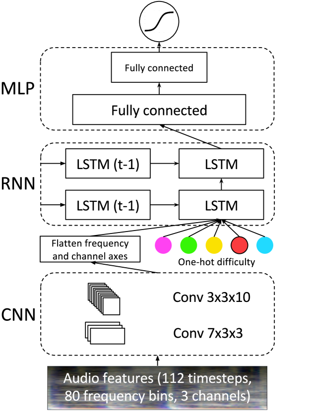
We consider several models to address the step placement task. Each model’s output consists of a single sigmoid unit which estimates the probability that a step is placed. For all models, we augment the audio features with a one-hot representation of difficulty.

Following state-of-the-art work on onset detection (Schlüter & Böck, 2014), we adopt a convolutional neural network (CNN) architecture. This model consists of two convolutional layers followed by two fully connected layers. Our first convolutional layer has 10 filter kernels that are 7-wide in time and 3-wide in frequency. The second layer has 20 filter kernels that are 3-wide in time and 3-wide in frequency. We apply 1D max-pooling after each convolutional layer, only in the frequency dimension, with a width and stride of 3. Both convolutional layers use rectified linear units (ReLU) (Glorot et al., 2011). Following the convolutional layers, we add two fully connected layers with rectifier activation functions and $256$ and $128$ nodes, respectively.

To improve upon the CNN, we propose a C-LSTM model, combining a convolutional encoding with an RNN that integrates information across longer windows of time. To encode the raw audio at each time step, we first apply two convolutional layers (of the same shape as the CNN) across the full unrolling length. The output of the second convolutional layer is a $3$D tensor, which we flatten along the channel and frequency axes (preserving the temporal dimension). The flattened features at each time step then become the inputs to a two-layer RNN.

The C-LSTM contains long short-term memory (LSTM) units (Hochreiter & Schmidhuber, 1997) with forget gates (Gers & Schmidhuber, 2000). The LSTM consists of $2$ layers with $200$ nodes each. Following the LSTM layers, we apply two fully connected ReLU layers of dimension $256$ and $128$. This architecture is depicted in Figure 5. We train this model using $100$ unrollings for backpropagation through time.

A chart’s intended difficulty influences decisions both about how many steps to place and where to place them. For low-difficulty charts, the average number of steps per second is less than one. In contrast, the highest-difficulty charts exceed seven steps per second. We trained all models both with and without conditioning on difficulty, and found the inclusion of this feature to be informative. We concatenate difficulty features to the flattened output of the CNN before feeding the vector to the fully connected (or LSTM) layers (Figure 5). We initialize weight matrices following the scheme of Glorot & Bengio (2010).

Training Methodology

We minimize binary cross-entropy with mini-batch stochastic gradient descent. For all models we train with batches of size $256$, scaling down gradients when their $l_{2}$ norm exceeds $5$. We apply $50\%$ dropout following each LSTM and fully connected layer. For LSTM layers, we apply dropout in the input to output but not temporal directions, following best practices from (Zaremba et al., 2014; Lipton et al., 2016; Dai & Le, 2015). Although the problem exhibits pronounced class imbalance (97% negatives), we achieved better results training on imbalanced data than with re-balancing schemes. We exclude all examples before the first step in the chart or after the last step as charts typically do not span the entire duration of the song.

For recurrent neural networks, the target at each frame is the ground truth value corresponding to that frame. We calculate updates using backpropagation through time with $100$ steps of unrolling, equal to one second of audio or two beats on a typical track ($120$ BPM). We train all networks with early-stopping determined by the area under the precision-recall curve on validation data. All models satisfy this criteria within $12$ hours of training on a single machine with an NVIDIA Tesla K40m GPU.

4.3 Peak Picking

Figure 6: One second of peak picking. Green: Ground truth region (A): true positive, (B): false positive, (C): false negative, (D): two peaks smoothed to one by Hamming window, (E): misaligned peak accepted as true positive by $\pm 20\mathit{ms}$ tolerance

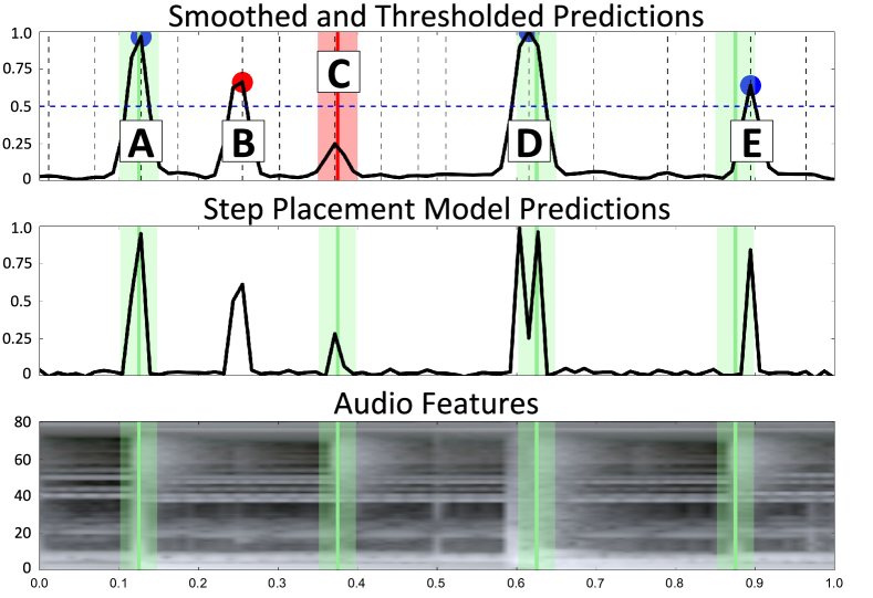
Following standard practice for onset detection, we convert sequences of step probabilities into a discrete set of chosen placements via a peak-picking process. First we run our step placement algorithm over an entire song to assign the probabilities of a step occurring within each $10\mathit{ms}$ frame. We then convolve this sequence of predicted probabilities with a Hamming window, smoothing the predictions and suppressing double-peaks from occurring within a short distance. Finally, we apply a constant threshold to choose which peaks are high enough (Figure 6). Because the number of peaks varies according to chart difficulty, we choose a different threshold per difficulty level. We consider predicted placements to be true positives if they lie within a $\pm 20\mathit{ms}$ window of a ground truth.

4.4 Step Selection

Figure 7: LSTM model used for step selection

We treat the step selection task as a sequence generation problem. Our approach follows related work in language modeling where RNNs are well-known to produce coherent text that captures long-range relationships (Mikolov et al., 2010; Sutskever et al., 2011; Sundermeyer et al., 2012).

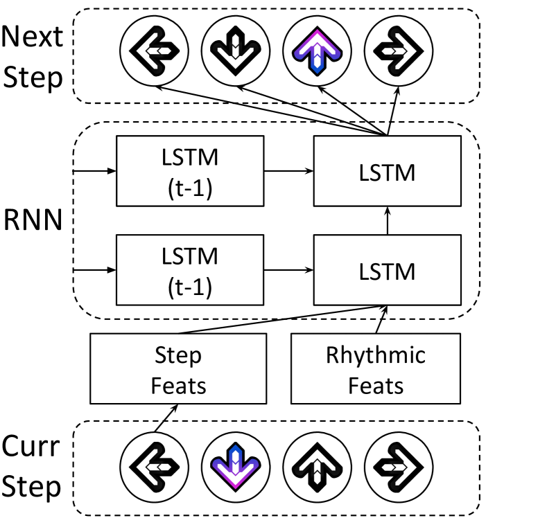
Our LSTM model passes over the ground truth step placements and predicts the next token given the previous sequence of tokens. The output is a softmax distribution over the $256$ possible steps. As input, we use a more compact bag-of-arrows representation containing $16$ features ($4$ per arrow) to depict the previous step. For each arrow, the $4$ corresponding features represent the states on, off, hold, and release. We found the bag-of-arrows to give equivalent performance to the one-hot representation while requiring fewer parameters. We add an additional feature that functions as a start token to denote the first step of a chart. For this task, we use an LSTM with $2$ layers of $128$ cells each.

Finally, we provide additional musical context to the step selection models by conditioning on rhythmic features (Figure 7). To inform models of the non-uniform spacing of the step placements, we consider the following three features: (1) $\Delta$-time adds two features representing the time since the previous step and the time until the next step; (2) $\Delta$-beat adds two features representing the number of beats since the previous and until the next step; (3) beat phase adds four features representing which 16th note subdivision of the beat the current step most closely aligns to.

Training Methodology

For all neural network models, we learn parameters by minimizing cross-entropy. We train with mini-batches of size $64$, and scale gradients using the same scheme as for step placement. We use $50\%$ dropout during training for both the MLP and RNN models in the same fashion as for step placement. We use $64$ steps of unrolling, representing an average of $100$ seconds for the easiest charts and $9$ seconds for the hardest. We apply early-stopping determined by average per-step cross entropy on validation data. All models satisfy this criteria within $6$ hours of training on a single machine with an NVIDIA Tesla K40m GPU.

5 Experiments

For both the Fraxtil and ITG datasets we apply $80\%$, $10\%$, $10\%$ splits for training, validation, and test data, respectively. Because of correlation between charts for the same song of varying difficulty, we ensure that all charts for a particular song are grouped together in the same split.

5.1 Step Placement

Table 2: Results for step placement experiments

Model	Dataset	PPL	AUC	F-scorec	F-scorem
LogReg	Fraxtil	1.205	0.601	0.609	0.667
MLP	Fraxtil	1.097	0.659	0.665	0.726
CNN	Fraxtil	1.082	0.671	0.678	0.750
C-LSTM	Fraxtil	1.070	0.682	0.681	0.756
LogReg	ITG	1.123	0.599	0.634	0.652
MLP	ITG	1.090	0.637	0.671	0.704
CNN	ITG	1.083	0.677	0.689	0.719
C-LSTM	ITG	1.072	0.680	0.697	0.721

Table 3: Results for step selection experiments

Model	Dataset	PPL	Accuracy
KN5	Fraxtil	3.681	0.528
MLP5	Fraxtil	3.744	0.543
MLP5 + $\Delta$-time	Fraxtil	3.495	0.553
MLP5 + $\Delta$-beat + beat phase	Fraxtil	3.428	0.557
LSTM5	Fraxtil	3.583	0.558
LSTM5 + $\Delta$-time	Fraxtil	3.188	0.584
LSTM5 + $\Delta$-beat + beat phase	Fraxtil	3.185	0.581
LSTM64	Fraxtil	3.352	0.578
LSTM64 + $\Delta$-time	Fraxtil	3.107	0.606
LSTM64 + $\Delta$-beat + beat phase	Fraxtil	3.011	0.613
KN5	ITG	5.847	0.356
MLP5	ITG	5.312	0.376
MLP5 + $\Delta$-time	ITG	4.792	0.402
MLP5 + $\Delta$-beat + beat phase	ITG	4.786	0.401
LSTM5	ITG	5.040	0.407
LSTM5 + $\Delta$-time	ITG	4.412	0.439
LSTM5 + $\Delta$-beat + beat phase	ITG	4.447	0.441
LSTM64	ITG	4.780	0.426
LSTM64 + $\Delta$-time	ITG	4.284	0.454
LSTM64 + $\Delta$-beat + beat phase	ITG	4.342	0.444

We evaluate the performance of our step placement methods against baselines via the methodology outlined below.

Baselines

To establish reasonable baselines for step placement, we first report the results of a logistic regressor (LogReg) trained on flattened audio features. We also report the performance of an MLP. Our MLP architecture contains two fully-connected layers of size 256 and 128, with rectifier nonlinearity applied to each layer. We apply dropout with probability $50\%$ after each fully-connected layer during training. We model our CNN baseline on the method of Schlüter & Böck (2014), a state-of-the-art algorithm for onset detection.

Metrics

We report each model’s perplexity (PPL) averaged across each frame in each chart in the test data. Using the sparse step placements, we calculate the average per-chart area under the precision-recall curve (AUC). We average the best per-chart F-scores and report this value as F-score^c. We calculate the micro F-score across all charts and report this value as F-score^m.

In Table 2, we list the results of our experiments for step placement. For ITG, models were conditioned on not just difficulty but also a one-hot representation of chart author. For both datasets, the C-LSTM model performs the best by all evaluation metrics. Our models achieve significantly higher F-scores for harder difficulty step charts. On the Fraxtil dataset, the C-LSTM achieves an F-score^c of $0.844$ for the hardest difficulty charts but only $0.389$ for the lowest difficulty. The difficult charts contribute more to F-score^m calculations because they have more ground truth positives. We discuss these results further in Section 6.

5.2 Step Selection

Baselines

For step selection, we compare the performance of the conditional LSTM to an $n$-gram model. Note that perplexity can be unbounded when a test set token is assigned probability $0$ by the generative model. To protect the $n$-gram models against unbounded loss on previously unseen $n$-grams, we use modified Kneser-Ney smoothing (Chen & Goodman, 1998), following best practices in language modeling (Mikolov et al., 2010; Sutskever et al., 2011). Specifically, we train a smoothed $5$-gram model with backoff (KN5) as implemented in Stolcke (2002).

Following the work of Bengio et al. (2003) we also compare against a fixed-window $5$-gram MLP which takes $4$ bag-of-arrows-encoded steps as input and predicts the next step. The MLP contains two fully-connected layers with $256$ and $128$ nodes and $50\%$ dropout after each layer during training. As with the LSTM, we train the MLP both with and without access to side features. In addition to the LSTM with 64 steps of unrolling, we train an LSTM with 5 steps of unrolling. These baselines show that the LSTM learns complex, long-range dependencies. They also demonstrate the discriminative information conferred by the $\Delta$-time, $\Delta$-beat, and beat phase features.

Metrics

We report the average per-step perplexity, averaging scores calculated separately on each chart. We also report a per-token accuracy. We calculate accuracy by comparing the ground-truth step to the argmax over a model’s predictive distribution given the previous sequence of ground-truth tokens. For a given chart, the per token accuracy is averaged across time steps. We produce final numbers by averaging scores across charts.

In Table 3 we present results for the step selection task. For the Fraxtil dataset, the best performing model was the LSTM conditioned on both $\Delta$-beat and beat phase, while for ITG it was the LSTM conditioned on $\Delta$-time. While conditioning on rhythm features was generally beneficial, the benefits of various features were not strictly additive. Representing $\Delta$-beat and $\Delta$-time as real numbers outperformed bucketed representations.

Additionally, we explored the possibility of incorporating more comprehensive representations of the audio into the step selection model. We considered a variety of representations, such as conditioning on CNN features learned from the step placement task. We also experimented with jointly learning a CNN audio encoder. In all cases, these approaches led to rapid overfitting and never approached the performance of the conditional LSTM generative model; perhaps a much larger dataset could support these approaches. Finally, we tried conditioning the step selection models on both difficulty and chart author but found these models to overfit quickly as well.

6 Discussion

Our experiments establish the feasibility of using machine learning to automatically generate high-quality DDR charts from raw audio. Our performance evaluations on both subtasks demonstrate the advantage of deep neural networks over classical approaches. For step placement, the best performing model is an LSTM with CNN encoder, an approach which has been used for speech recognition (Amodei et al., 2015), but, to our knowledge, never for music-related tasks. We noticed that by all metrics, our models perform better on higher-difficulty charts. Likely, this owes to the comparative class imbalance of the lower difficulty charts.

Figure 8: Top: A real step chart from the Fraxtil dataset on the song Anamanaguchi - Mess. Middle: One-step lookahead predictions for the LSTM model, given Fraxtil’s choreography as input. The model predicts the next step with high accuracy (errors in red). Bottom: Choreography generated by conditional LSTM model.

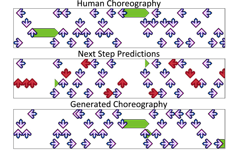
The superior performance of LSTMs over fixed-window approaches on step selection suggests both that DDR charts exhibit long range dependencies and that recurrent neural networks can exploit this complex structure. In addition to reporting quantitative results, we visualize the step selection model’s next-step predictions. Here, we give the entire ground truth sequence as input but show the predicted next step at each time. We also visualize a generated choreography, where each sampled output from the LSTM is fed in as the subsequent input (Figure 8). We note the high accuracy of the model’s predictions and qualitative similarity of the generated sequence to Fraxtil’s choreography.

For step selection, we notice that modeling the Fraxtil dataset choreography appears to be easy compared to the multi-author ITG dataset. We believe this owes to the distinctiveness of author styles. Because we have so many step charts for Fraxtil, the network is able to closely mimic his patterns. While the ITG dataset contains multiple charts per author, none are so prolific as Fraxtil.

We released a public demo using our most promising models as measured by our quantitative evaluation. Players upload an audio file, select a difficulty rating and receive a step chart for use in the StepMania DDR simulator. Our demo produces a step chart for a $3$ minute song in about $5$ seconds using an NVIDIA Tesla K40c GPU. At time of writing, $220$ players have produced $1370$ step charts with the demo. We also solicited feedback, on a scale of $1$-$5$, for player “satisfaction” with the demo results. The $22$ respondents reported an average satisfaction of $3.87$.

A promising direction for future work is to make the selection algorithm audio-aware. We know qualitatively that elements in the ground truth choreography tend to coincide with specific musical events: jumps are used to emphasize accents in a rhythm; freezes are used to transition from regions of high rhythmic intensity to more ambient sections.

DDR choreography might also benefit from an end-to-end approach, in which a model simultaneously places steps and selects them. The primary obstacle here is data sparsity at any sufficiently high feature rate. At $100\mathit{Hz}$, about $97\%$ of labels are null. So in $100$ time-steps of unrolling, an RNN might only encounter $3$ ground truth steps.

We demonstrate that step selection methods are improved by incorporating $\Delta$-beat and beat phase features, however our current pipeline does not produce this information. In lieu of manual tempo input, we are restricted to using $\Delta$-time features when executing our pipeline on unseen recordings. If we trained a model to detect beat phase, we would be able to use these features for step selection.

7 Related Work

Several academic papers address DDR. These include anthropological studies (Hoysniemi, 2006; Behrenshausen, 2007) and two papers that describe approaches to automated choreography. The first, called Dancing Monkeys, uses rule-based methods for both step placement and step selection (O’Keeffe, 2003). The second employs genetic algorithms for step selection, optimizing an ad-hoc fitness function (Nogaj, 2005). Neither establishes reproducible evaluation methodology or learns the semantics of steps from data.

Our step placement task closely resembles the classic problem of musical onset detection (Bello et al., 2005; Dixon, 2006). Several onset detection papers investigate modern deep learning methodology. Eyben et al. (2010) employ bidirectional LSTMs (BLSTMs) for onset detection; Marchi et al. (2014) improve upon this work, developing a rich multi-resolution feature representation; Schlüter & Böck (2014) demonstrate a CNN-based approach (against which we compare) that performs competitively with the prior BLSTM work. Neural networks are widely used on a range of other MIR tasks, including musical chord detection (Humphrey & Bello, 2012; Boulanger-Lewandowski et al., 2013a) and boundary detection (Ullrich et al., 2014), another transient audio phenomenon.

Our step selection problem resembles the classic natural language processing task of statistical language modeling. Classical methods, which we consider, include $n$-gram distributions (Chen & Goodman, 1998; Rosenfeld, 2000). Bengio et al. (2003) demonstrate an approach to language modeling using neural networks with fixed-length context. More recently, RNNs have demonstrated superior performance to fixed-window approaches (Mikolov et al., 2010; Sundermeyer et al., 2012; Sutskever et al., 2011). LSTMs are also capable of modeling language at the character level (Karpathy et al., 2015; Kim et al., 2016). While a thorough explanation of modern RNNs exceeds the scope of this paper, we point to two comprehensive reviews of the literature (Lipton et al., 2015; Greff et al., 2016). Several papers investigate neural networks for single-note melody generation (Bharucha & Todd, 1989; Eck, 2002; Chu et al., 2016; Hadjeres & Pachet, 2016) and polyphonic melody generation (Boulanger-Lewandowski et al., 2012).

Learning to choreograph requires predicting both the timing and the type of events in relation to a piece of music. In that respect, our task is similar to audio sequence transduction tasks, such as musical transcription and speech recognition. RNNs currently yield state-of-the-art performance for musical transcription (Böck & Schedl, 2012; Boulanger-Lewandowski et al., 2013b; Sigtia et al., 2016). RNNs are widely used for speech recognition (Graves & Jaitly, 2014; Graves et al., 2006, 2013; Sainath et al., 2015), and the state-of-the-art method (Amodei et al., 2015) combines convolutional and recurrent networks. While our work is methodologically similar, it differs from the above in that we consider an entirely different application.

8 Conclusions

By combining insights from musical onset detection and statistical language modeling, we have designed and evaluated a number of deep learning methods for learning to choreograph. We have introduced standardized datasets and reproducible evaluation methodology in the hope of encouraging wider investigation into this and related problems. We emphasize that the sheer volume of available step charts presents a rare opportunity for MIR: access to large amounts of high-quality annotated data. This data could help to spur innovation for several MIR tasks, including onset detection, beat tracking, and tempo detection.

References

- Amodei et al. (2015) Amodei, Dario, Anubhai, Rishita, Battenberg, Eric, Case, Carl, Casper, Jared, Catanzaro, Bryan, Chen, Jingdong, Chrzanowski, Mike, Coates, Adam, Diamos, Greg, et al. Deep speech 2: End-to-end speech recognition in english and mandarin. In ICML, 2015.
- Behrenshausen (2007) Behrenshausen, Bryan G. Toward a (kin) aesthetic of video gaming the case of dance dance revolution. Games and Culture, 2007.
- Bello et al. (2005) Bello, Juan Pablo, Daudet, Laurent, Abdallah, Samer, Duxbury, Chris, Davies, Mike, and Sandler, Mark B. A tutorial on onset detection in music signals. IEEE Transactions on speech and audio processing, 2005.
- Bengio et al. (2003) Bengio, Yoshua, Ducharme, Réjean, Vincent, Pascal, and Jauvin, Christian. A neural probabilistic language model. JMLR, 2003.
- Bharucha & Todd (1989) Bharucha, Jamshed J and Todd, Peter M. Modeling the perception of tonal structure with neural nets. Computer Music Journal, 1989.
- Böck & Schedl (2012) Böck, Sebastian and Schedl, Markus. Polyphonic piano note transcription with recurrent neural networks. In ICASSP, 2012.
- Bogdanov et al. (2013) Bogdanov, Dmitry, Wack, Nicolas, Gómez, Emilia, Gulati, Sankalp, Herrera, Perfecto, Mayor, Oscar, Roma, Gerard, Salamon, Justin, Zapata, José R, and Serra, Xavier. Essentia: An audio analysis library for music information retrieval. In ISMIR, 2013.
- Boulanger-Lewandowski et al. (2012) Boulanger-Lewandowski, Nicolas, Bengio, Yoshua, and Vincent, Pascal. Modeling temporal dependencies in high-dimensional sequences: Application to polyphonic music generation and transcription. In ICML, 2012.
- Boulanger-Lewandowski et al. (2013a) Boulanger-Lewandowski, Nicolas, Bengio, Yoshua, and Vincent, Pascal. Audio chord recognition with recurrent neural networks. In ISMIR, 2013a.
- Boulanger-Lewandowski et al. (2013b) Boulanger-Lewandowski, Nicolas, Bengio, Yoshua, and Vincent, Pascal. High-dimensional sequence transduction. In ICASSP, 2013b.
- Chen & Goodman (1998) Chen, Stanley F and Goodman, Joshua. An empirical study of smoothing techniques for language modeling. Technical Report TR-10-98, Harvard University, 1998.
- Chu et al. (2016) Chu, Hang, Urtasun, Raquel, and Fidler, Sanja. Song from pi: A musically plausible network for pop music generation. arXiv:1611.03477, 2016.
- Dai & Le (2015) Dai, Andrew M and Le, Quoc V. Semi-supervised sequence learning. In NIPS, 2015.
- Dixon (2006) Dixon, Simon. Onset detection revisited. In Proceedings of the 9th International Conference on Digital Audio Effects, 2006.
- Eck (2002) Eck, Douglas. A first look at music composition using lstm recurrent neural networks. Technical Report IDSIA-07-02, 2002.
- Eyben et al. (2010) Eyben, Florian, Böck, Sebastian, Schuller, Björn W, and Graves, Alex. Universal onset detection with bidirectional long short-term memory neural networks. In ISMIR, 2010.
- Gers & Schmidhuber (2000) Gers, Felix and Schmidhuber, Jürgen. Recurrent nets that time and count. In International Joint Conference on Neural Networks (IJCNN), 2000.
- Glorot & Bengio (2010) Glorot, Xavier and Bengio, Yoshua. Understanding the difficulty of training deep feedforward neural networks. In AISTATS, 2010.
- Glorot et al. (2011) Glorot, Xavier, Bordes, Antoine, and Bengio, Yoshua. Deep sparse rectifier neural networks. In AISTATS, 2011.
- Graves & Jaitly (2014) Graves, Alex and Jaitly, Navdeep. Towards end-to-end speech recognition with recurrent neural networks. In ICML, 2014.
- Graves et al. (2006) Graves, Alex, Fernández, Santiago, Gomez, Faustino, and Schmidhuber, Jürgen. Connectionist temporal classification: labelling unsegmented sequence data with recurrent neural networks. In ICML, 2006.
- Graves et al. (2013) Graves, Alex, Mohamed, Abdel-rahman, and Hinton, Geoffrey. Speech recognition with deep recurrent neural networks. In ICASSP, 2013.
- Greff et al. (2016) Greff, Klaus, Srivastava, Rupesh K, Koutník, Jan, Steunebrink, Bas R, and Schmidhuber, Jürgen. Lstm: A search space odyssey. IEEE transactions on neural networks and learning systems, 2016.
- Hadjeres & Pachet (2016) Hadjeres, Gaëtan and Pachet, François. Deepbach: a steerable model for bach chorales generation. arXiv:1612.01010, 2016.
- Hamel et al. (2012) Hamel, Philippe, Bengio, Yoshua, and Eck, Douglas. Building musically-relevant audio features through multiple timescale representations. In ISMIR, 2012.
- Hochreiter & Schmidhuber (1997) Hochreiter, Sepp and Schmidhuber, Jürgen. Long short-term memory. Neural computation, 1997.
- Hoysniemi (2006) Hoysniemi, Johanna. International survey on the dance dance revolution game. Computers in Entertainment (CIE), 2006.
- Humphrey & Bello (2012) Humphrey, Eric J and Bello, Juan Pablo. Rethinking automatic chord recognition with convolutional neural networks. In ICMLA, 2012.
- Karpathy et al. (2015) Karpathy, Andrej, Johnson, Justin, and Fei-Fei, Li. Visualizing and understanding recurrent networks. arXiv:1506.02078, 2015.
- Kim et al. (2016) Kim, Yoon, Jernite, Yacine, Sontag, David, and Rush, Alexander M. Character-aware neural language models. In Proceedings of the Thirtieth AAAI Conference on Artificial Intelligence, 2016.
- Lipton et al. (2015) Lipton, Zachary C, Berkowitz, John, and Elkan, Charles. A critical review of recurrent neural networks for sequence learning. arXiv:1506.00019, 2015.
- Lipton et al. (2016) Lipton, Zachary C, Kale, David C, Elkan, Charles, and Wetzell, Randall. Learning to diagnose with LSTM recurrent neural networks. In ICLR, 2016.
- Marchi et al. (2014) Marchi, Erik, Ferroni, Giacomo, Eyben, Florian, Gabrielli, Leonardo, Squartini, Stefano, and Schuller, Bjorn. Multi-resolution linear prediction based features for audio onset detection with bidirectional lstm neural networks. IEEE, 2014.
- Mikolov et al. (2010) Mikolov, Tomas, Karafiát, Martin, Burget, Lukas, Cernockỳ, Jan, and Khudanpur, Sanjeev. Recurrent neural network based language model. In Interspeech, 2010.
- Nogaj (2005) Nogaj, Adam. A genetic algorithm for determining optimal step patterns in dance dance revolution. Technical report, State University of New York at Fredonia, 2005.
- O’Keeffe (2003) O’Keeffe, Karl. Dancing monkeys (automated creation of step files for dance dance revolution). Technical report, Imperial College London, 2003.
- Rosenfeld (2000) Rosenfeld, Ronald. Two decades of statistical language modeling: Where do we go from here? Proceedings of the IEEE, 2000.
- Sainath et al. (2015) Sainath, Tara N, Weiss, Ron J, Senior, Andrew, Wilson, Kevin W, and Vinyals, Oriol. Learning the speech front-end with raw waveform cldnns. In Interspeech, 2015.
- Schlüter & Böck (2014) Schlüter, Jan and Böck, Sebastian. Improved musical onset detection with convolutional neural networks. In ICASSP, 2014.
- Sigtia et al. (2016) Sigtia, Siddharth, Benetos, Emmanouil, and Dixon, Simon. An end-to-end neural network for polyphonic piano music transcription. IEEE/ACM Transactions on Audio, Speech, and Language Processing, 2016.
- Stevens et al. (1937) Stevens, Stanley Smith, Volkmann, John, and Newman, Edwin B. A scale for the measurement of the psychological magnitude pitch. The Journal of the Acoustical Society of America, 1937.
- Stolcke (2002) Stolcke, Andreas. Srilm-an extensible language modeling toolkit. In Interspeech, 2002.
- Sundermeyer et al. (2012) Sundermeyer, Martin, Schlüter, Ralf, and Ney, Hermann. Lstm neural networks for language modeling. In Interspeech, 2012.
- Sutskever et al. (2011) Sutskever, Ilya, Martens, James, and Hinton, Geoffrey E. Generating text with recurrent neural networks. In ICML, 2011.
- Towns et al. (2014) Towns, John, Cockerill, Timothy, Dahan, Maytal, Foster, Ian, Gaither, Kelly, Grimshaw, Andrew, Hazlewood, Victor, Lathrop, Scott, Lifka, Dave, Peterson, Gregory D, et al. Xsede: accelerating scientific discovery. Computing in Science & Engineering, 2014.
- Ullrich et al. (2014) Ullrich, Karen, Schlüter, Jan, and Grill, Thomas. Boundary detection in music structure analysis using convolutional neural networks. In ISMIR, 2014.
- Zaremba et al. (2014) Zaremba, Wojciech, Sutskever, Ilya, and Vinyals, Oriol. Recurrent neural network regularization. arXiv:1409.2329, 2014.