Are LIGO’s Black Holes Made From Smaller Black Holes?
Abstract
One proposed formation channel for stellar mass black holes (BHs) is through hierarchical mergers of smaller BHs. Repeated mergers between comparable mass BHs leave an imprint on the spin of the resulting BH, since the final BH spin is largely determined by the orbital angular momentum of the binary. We find that for stellar mass BHs forming hierarchically the distribution of spin magnitudes is universal, with a peak at and little support below . We show that the spin distribution is robust against changes to the mass ratio of the merging binaries, the initial spin distribution of the first generation of BHs, and the number of merger generations. While we assume an isotropic distribution of initial spin directions, spins that are preferentially aligned or antialigned do not qualitatively change our results. We also consider a “cluster catastrophe” model for BH formation in which we allow for mergers of arbitrary mass ratios and show that this scenario predicts a unique spin distribution that is similar to the universal distribution derived for major majors. We explore the ability of spin measurements from ground-based gravitational-wave (GW) detectors to constrain hierarchical merger scenarios. We apply a hierarchical Bayesian mixture model to mock GW data and argue that the fraction of BHs that formed through hierarchical mergers will be constrained with LIGO binary black hole detections, while with detections we could falsify a model in which all component BHs form hierarchically.
1. Introduction
LIGO’s first detections of gravitational waves (GWs) from binary black hole (BBH) systems allow us to probe the formation histories of stellar mass binary black holes (BHs; Abbott et al., 2016a). Various formation channels have been proposed for the component black holes in these binaries (Belczynski et al., 2016; Rodriguez et al., 2016b; de Mink & Mandel, 2016; Bird et al., 2016; Clesse & García-Bellido, 2017; Antonini & Rasio, 2016; Inayoshi et al., 2017), and these can be broadly separated into two classes: isolated binary evolution and dynamical binary formation channels that involve first-generation BHs (e.g., resulting from stellar collapse) and dynamical formation channels that involve BHs built up from the mergers of earlier generations of BHs. In this work, we consider the latter group: BH formation through hierarchical mergers wherein a BH in a BH binary is produced by a merger of two smaller BHs from a previous generation, and the previous generation’s BHs may themselves be merger products of an even earlier generation. Hierarchical mergers may occur in high-density environments where some fraction of merger products do not escape despite receiving recoil kicks (Merritt et al., 2004) and may therefore undergo another merger. The hierarchical merger scenario has been proposed in the context of dynamical formation in nuclear star clusters (Antonini & Rasio, 2016), young stellar clusters (Mapelli, 2016), AGN disks (McKernan et al., 2017), as well as in the formation of primordial BHs (Clesse & García-Bellido, 2017).
In anticipation of future LIGO BBH detections, we describe a method to determine whether or not the observed BHs formed hierarchically. In particular, the hierarchical formation channel can be probed by analyzing the distribution of observed spin magnitudes of the component BHs.
Each BH in a binary has a mass and spin
| (1) |
where is the dimensionless spin magnitude and is the unit spin vector. Because the spins of the BHs in a binary system influence the dynamics of the inspiral and merger, a GW detection provides a measurement of the component spins (Abbott et al., 2016b).
For an individual GW event, the spin measurements are often poorly constrained (Vitale et al., 2014; Pürrer et al., 2016), but we can combine individual spin posteriors to examine the distribution of dimensionless spin magnitudes across all events. In this Letter, we show that the hierarchical merger scenario yields a unique distribution of BH spin magnitudes ; therefore, by measuring the spins of observed systems, we can constrain this formation process. Our approach is complementary to that of Gerosa & Berti (2017), who study the expected distributions of mass, redshift, and binary spin parameter for populations of first- and second-generation BHs and show how to use all three measurements to constrain the fraction of second-generation BHs in a detected population. In contrast, we focus solely on GW measurements of spin magnitude and consider arbitrary generations of previous mergers.
To construct the distribution of BH spin magnitudes resulting from hierarchical mergers, we utilize previous studies of the evolution of BH spins through binary coalescence. Due to advancements in numerical relativity (NR) and post-Newtonian (PN) methods, a number of groups have developed reliable formulae for the final spin following a merger of two spinning BHs (Buonanno et al., 2008; Kesden, 2008; Tichy & Marronetti, 2008; Healy et al., 2014; Hofmann et al., 2016; Jiménez-Forteza et al., 2017). Intuitively, there are two contributions to the spin following a coalescence: the individual spins of the two progenitor BHs and the binary system’s orbital angular momentum. As the BBHs inspiral toward each other, they lose energy and orbital angular momentum through the emission of GWs. When the Bus finally merge, as shown by Buonanno et al. (2008), the remaining orbital angular momentum that contributes to the final BH spin can be approximated by the orbital angular momentum of a test particle at the innermost stable circular orbit of the final BH (where the mass of the test particle is taken to be the reduced mass of the BBHs). The contribution from the orbital angular momentum will be most significant for equal mass BBHs and will dominate over the contribution from the spin angular momentum. For example, as is well understood from NR simulations, a merger of nonspinning BBHs of equal mass will result in a final BH with a dimensionless spin magnitude of (Hofmann et al., 2016). In order for the spins of the BBHs to cancel the orbital angular momentum, resulting in a nonspinning BH, the spins must be sufficiently large and antialigned to the orbital angular momentum, and the mass ratio must be sufficiently small. In fact, using the results of Buonanno et al. (2008), the antialigned contributions to the spins, , , and the mass ratio, , must satisfy
| (2) |
in order to end up with a nonspinning BH. Thus, even for maximally antialigned spins, the mass ratio must satisfy in order to overwhelm the orbital angular momentum. As we shall see, this explains why major mergers (in which ) result in BHs with a relatively high spin distribution, peaked at , and with little support below .
In this work, we consider major mergers () as the basis of the hierarchical merger scenario. If the BHs of each generation interact with each other dynamically, they are more likely to form binaries with BHs of similar mass (Sigurdsson & Hernquist, 1993; Rodriguez et al., 2016b) and we would expect mergers of near-equal mass BHs (Rodriguez et al., 2016a; O’Leary et al., 2016). We would similarly expect near-unity mass ratios for BBHs of primordial origin, as PBH formation scenarios generally allow a narrow mass range for the first generation (Kovetz et al., 2016), and we assume that because of dynamical considerations, such BHs only merge with partners of the same generation.
The assumption of major mergers differs from the seminal work of Hughes & Blandford (2003), which considered the spin evolution of supermassive BHs as they grow through minor mergers. In contrast to major mergers, minor mergers tend to decrease the spin of the final BH, because the binary’s orbital angular momentum is smallest when it augments the total BBH spins (a prograde orbit) and largest when it counteracts it (a retrograde orbit).
We also assume that, in the absence of any aligning mechanism, the spins of each generation of BHs in the hierarchical merger scenario are isotropically distributed on the sphere. The effects of BBH spins that are preferentially aligned or antialigned with the orbital angular momentum are discussed in Section 3. However, it is important to note that spins that are initially partially aligned (antialigned) with the orbital angular momentum can become significantly antialigned (aligned) during the inspiral due to precession (Kesden et al., 2010). This will not affect an isotropic distribution of spins, as a distribution of spins that is isotropic at large distances will remain isotropic during the inspiral up to the point of plunge (Kesden et al., 2010). Furthermore, the magnitudes of the BBH spins remain nearly constant during the inspiral (up to 2PN order), which further lends confidence to our calculation of the hierarchical merger spin distribution.
2. Methods
2.1. Hierarchical Merger Spin Distribution
We apply the formulas of Hofmann et al. (2016) to predict the final BH spin from a merger of two BHs, given the spin vectors and masses of the component BHs. This allows us to build a statistical distribution of spin magnitudes resulting from hierarchical mergers, similar to the distributions found by Tichy & Marronetti (2008) and Lousto et al. (2010).
Although we assume major mergers and isotropically distributed spin orientations, we wish to remain general with respect to other aspects of the hierarchical merger scenario. In particular, we do not at the outset specify the spin distribution of the first generation of BHs (before any mergers have occurred) or the exact distribution of mass ratios of merging BHs (although we limit ourselves to ). Furthermore, the desired spin distribution presumably evolves as each generation’s BHs merge to form the next generation, but we do not wish to restrict ourselves to a particular generation of the hierarchical merger scenario. Fortunately, as we show below, the resulting spin distribution is relatively insensitive to the spin magnitudes of the first generation, the mass ratios (within the range ), or which generation we consider (starting with the second generation). We demonstrate this explicitly by computing spin distributions under various choices of these parameters.
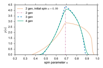
We compute probability density functions of dimensionless spin magnitudes as follows: we start by taking a large () ensemble of BHs, and then randomly pick pairs of BHs from this first generation and merge each pair, calculating the final spin from the Hofmann et al. (2016) formula. This gives us the distribution of spin magnitudes for the second generation of BHs. In the simplest case we take the first generation of BHs to be all of the same mass and nonspinning, in which case, the second generation’s BHs will all be of roughly double the mass and spinning with dimensionless spin magnitude . If the initial generation of BHs is equal mass but with isotropic, near-maximal () spins, the second generation of BHs will have a distribution of spin magnitudes that is similarly peaked at with slightly wider support (see Fig. 1).
To calculate the spin distribution for the third generation of BHs, we randomly and repeatedly choose pairs of BH spin magnitudes from the second generation and randomly choose their spin directions from a spherically isotropic distribution. This yields the spin magnitudes of the third generation of BHs, and we can iterate this procedure to calculate the distribution of BH spins for the th generation given the distribution of spins for the th generation. In practice, we find that the spin distribution changes only slightly between the third and the fourth generation and has fully converged by the fourth generation, regardless of the initial spin distribution (see Fig. 1). Different choices of initial spin lead to indistinguishable spin distributions by the third generation.
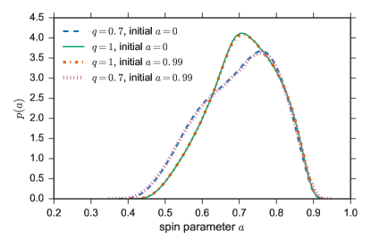
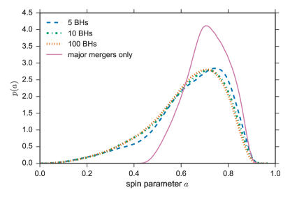
To explore the effect of different mass ratios, we consider a toy model in which all mergers occur with a mass ratio of , instead of as assumed above. We find that the resulting spin distributions are very similar (see Fig. 2), suggesting that any distribution of mass ratios in the range (as expected for dynamically forming binaries) would not significantly affect the distribution of final spins. Thus, we find that regardless of mass ratio and initial spin, the hierarchical merger scenario gives rise to a single, standard distribution of BH dimensionless spin magnitudes sharply peaked at with nonzero support over . In what follows when we refer to the hierarchical merger spin distribution, we mean the distribution shown in Fig. 2, calculated as the fourth generation of equal mass mergers. An alternate choice would not significantly affect our results.
Our findings are consistent with Berti & Volonteri (2008), who found that following a single merger the final spin magnitude is regardless of the initial spin magnitude, assuming we average over an isotropic distribution of spin directions (see their Fig. 2). Our results are also consistent with Tichy & Marronetti (2008) and Lousto et al. (2010), both of whom found that the distribution of spin magnitudes converges after four generations of repeated mergers. However, note that by limiting ourselves to the major mergers relevant for stellar mass BHs, our hierarchical merger spin distribution is different from the distribution presented in Fig. 19 of Lousto et al. (2010), as they considered a wide distribution of mass ratios appropriate for supermassive BHs. In particular, our distribution has little support below . Our hierarchical merger spin distribution is most similar to the distribution in Fig. 1 of Tichy & Marronetti (2008) and Fig. 20 of Lousto et al. (2010); however, we argue that this distribution is insensitive to the initial BH spins and is an adequate description of the second and third generation of BHs even before it fully converges in the fourth generation.
2.2. Mixture Model Analysis
We apply a hierarchical Bayesian framework (Hogg et al., 2010; Mandel et al., 2011) to analyze a collection of BH spin measurements, where the spin measurement from the th GW detection takes the form of a two-dimensional posterior for the BBH spin magnitudes , where and is the data. To understand the true population of BH spins from the observed BBHs, we assume that the true spin distribution is parameterized in terms of some parameters, , which we seek to infer. The true spin distribution, therefore, can be written as , and we want to know , where is the data across all GW detections. We assume that each GW detection is independent, so that
| (3) |
Furthermore, we have
| (4) |
and applying Bayes’s rule gives
| (5) |
where is the two-dimensional likelihood for the BBH spins, and is the prior probability for the population parameters . Before we have learned anything about the population distribution of spin magnitudes , in the analysis of individual events, we assume a two-dimensional flat prior on , so that the likelihood is proportional to the posterior . Putting together equations 3–5, we have
| (6) |
where, because for a single event, we can evaluate the above integral over of weighed by the likelihood as an average over posterior samples :
| (7) | ||||
In our case, in order to investigate whether the detected BBHs favor the hierarchical merger scenario, we write the true spin population as a mixture model. Lacking a strong astrophysical prior on the distribution of BH spins (Miller & Miller, 2015), we take some fraction of the BHs to be uniformly spinning over the allowed range , and the remaining of the BHs to come from the hierarchical merger population. It is straightforward to consider alternate spin magnitude distributions, and the same analysis would apply if we included an additional component in the mixture model or replaced the uniformly distributed component with a different spin distribution. For the mixture model with parameter , we have
| (8) |
where is the hierarchical merger spin distribution. We assume the spins of the BBHs in a single system are independent of one another, so
| (9) |
We also use a flat prior for the mixture parameter
| (10) |
Then for the mixture model, equation 6 becomes
| (11) | ||||
Using equation 7, given posterior samples for each BBH, we can approximate equation 11 as
| (12) | ||||
The mixture model parameterization provides a convenient way to compare the hierarchical merger model to any other model (in our case, a model that yields a flat distribution of spins). As Vitale et al. (2017) discuss, for a mixture of two (or more) models, we can write the posterior of the mixture parameter in terms of the Bayesian evidence for the models under consideration. In our case, we can relate the posterior to the evidence ratio, or Bayes factor, between the hierarchical merger model and the uniform spin model . The evidence for each model given data is defined as and , and, assuming GW detections are independent, we can write
| (13) | ||||
| (14) | ||||
| (15) | ||||
| (16) | ||||
| (17) |
We therefore have that the Bayes’s factor is
| (18) |
Thus, computing allows us to directly find the Bayes’s factor, which allows us to argue (or refute) that a population of observed BHs came from the hierarchical merger formation channel. The mixture model is also useful to constrain the fraction of the observations that are consistent with having formed through hierarchical mergers. In the next section, we demonstrate that this analysis will yield meaningful constraints within just a few years of advanced LIGO operation.
3. Results
For the purposes of this work, we illustrate our method on very simplified spin posterior distributions, leaving the analysis of real data to the LIGO collaboration. We assume that each BBH detection provides a measurement of the two component BH spin magnitudes with some uncertainty (see, for example, Fig. 5 of Abbott et al., 2016b). We neglect correlations between the two spin measurements, which is equivalent to setting
| (19) |
in equation 11. Following Stevenson et al. (2017), we approximate each spin magnitude posterior as a Gaussian, restricted to the range [0,1], with a standard deviation corresponding to the measurement uncertainty. In other words, for a BH with dimensionless spin magnitude , we generate a posterior centered on where is a random measurement error chosen from . The spin magnitude posterior for a single BH is then given by
| (20) |
truncated and normalized to our prior range . With these assumptions, we compute equation 11 by drawing 1000 samples from each spin magnitude posterior given by equation 20 for a simulated population of . In other words, we solve
| (21) |
where
| (22) |
for .
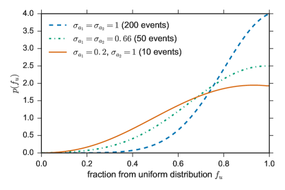
The uncertainty on spin magnitude depends on various factors, including the true spin magnitudes, the signal-to-noise ratio (SNR) of the inspiral and ringdown, the mass ratio of the binary, and the orientation of the spin vectors. As demonstrated by Pürrer et al. (2016), we expect this uncertainty to be rather large and not particularly dependent on the SNR, especially for events where there is little power in the ringdown, so we carry out our analysis with the conservative choice of We then repeat the analysis under the assumption that all events are like GW150914 in terms of spin magnitude uncertainty: consisting of one relatively well measured BH spin magnitude with , and one poorly measured BH spin magnitude with . This can be expected for events with moderately high SNR in both the inspiral (which constrains the weighted aligned spin combination ) and the ringdown (which constrains the spin of the final BH ). Motivated by the choice of posterior uncertainties in Stevenson et al. (2017) and an examination of mass ratio uncertainties and covariances for published LIGO events (see Table 1 and Fig. 4 of Abbott et al., 2016b), we repeat our analysis for spin posteriors with .
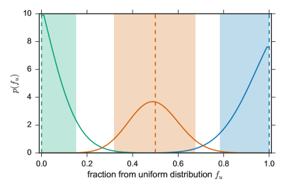
Our results are similar for all choices of spin magnitude uncertainties, suggesting that LIGO will be able to clearly distinguish between a population of hierarchically formed BHs and a population of uniformly spinning BHs with detections (see Fig. 4), although this will be possible with as few as 10 detections if at least one spin component is relatively well-measured () as in the case of GW150914 (see Fig. 3). If the true population of detected BHs is mixed, it requires more detections to precisely measure the fraction that have spin magnitudes consistent with formation through hierarchical mergers. We see in Fig. 4 that the confidence interval for is relatively wide for a mixed population with 400 events, although if we are simply interested in ruling out or , detections is sufficient even in the most pessimistic case considered. It is straightforward to extrapolate these results to a greater number of detections: as expected, the width of the posterior decreases with the number of detections, , as .
We have thus far analyzed the characteristic spin distribution resulting from major () mergers of isotropically spinning BHs. Below, we discuss the implications of relaxing these assumptions. We might expect deviations from isotropic spins in certain astrophysical situations such as BBH formation in a gas-rich AGN disk, where the spins of the component BHs can be preferentially aligned or antialigned with the orbital angular momentum (McKernan et al., 2017). If the spins of BBHs are always aligned with the orbital angular momentum, it is straightforward to see that this will result in an even narrower spin distribution, strongly peaked at very high spin magnitudes, converging to by the third generation. This situation will thus be easier to constrain with LIGO data. If both component spins are always antialigned with the orbital angular momentum and the first generation has moderately high spins , the future generations will have spins . Even assuming maximal antialigned initial spins, while the second-generation products will be spinning at for mass ratios , the spin distribution will converge to starting with the third generation. If the spins are equal in magnitude but one is aligned and the other antialigned with the orbital angular momentum, the situation is identical to a merger of nonspinning BHs and yields a spin magnitude (although note that the best-constrained spin parameter for the binary will be ). We conclude that hierarchical major mergers of BBHs cannot produce low spin magnitudes ().
We can relax the assumption of major mergers by considering an alternative “cluster catastrophe” formation scenario in which a fixed number, , of equal mass BHs repeatedly merge in randomly chosen pairs, irrespective of the mass ratio, until there is a single remaining BH. We take the initial distribution of spin magnitudes to be uniform in and spin directions to always be isotropic. We find that the spin magnitude of the single remaining BH is insensitive to or the initial spin magnitudes and is distributed according to the probability distribution in Fig. 5. While such a scenario can lead to low mass-ratio mergers in which the primary spin may cancel the orbital angular momentum and produce spin magnitudes , these low spin magnitudes remain unlikely: spin magnitudes are produced less than of the time.
4. Summary
We have shown that if BHs build up through hierarchical major mergers of smaller BHs, the spin magnitudes of the resulting BHs follow a universal distribution (see Fig. 2). Because this distribution is relatively independent of the details of the hierarchical merger scenario, we can use it to test whether an observed population of BHs was formed through hierarchical mergers. Although a GW observation of a single coalescing BBH does not strongly constrain individual BH spins (Abbott et al., 2016b), we estimate that the hierarchical formation channel will be strongly constrained with detections. Furthermore, we have shown that hierarchical mergers rarely produce BHs with spins below , and even in extreme scenarios that favor antialigned spins or result in a “cluster catastrophe," one rarely finds BH spins below . If BHs do not form through hierarchical mergers and the spin distribution is uniform on [0,1], we have shown that it will be possible to rule out the hierarchical formation channel with a sample of detections (see Fig. 3). If instead we select between a hierarchical model and one that favors low spins (instead of uniform as done above), even fewer detections would be sufficient to falsify either model. We note that the spin constraints of the primary component BHs of GW150914 and LVT151012 appear to favor spins over spins (see Figs. 5 of Abbott et al., 2016c, Abbott et al., 2016b), suggesting that they are unlikely to have formed through hierarchical major mergers. We leave a quantitative analysis of these events for future work.
References
- Abbott et al. (2016a) Abbott, B. P., Abbott, R., Abbott, T. D., et al. 2016a, ApJ, 818, L22
- Abbott et al. (2016b) —. 2016b, Physical Review X, 6, 041015
- Abbott et al. (2016c) —. 2016c, Physical Review Letters, 116, 241102
- Antonini & Rasio (2016) Antonini, F., & Rasio, F. A. 2016, ApJ, 831, 187
- Belczynski et al. (2016) Belczynski, K., Holz, D. E., Bulik, T., & O’Shaughnessy, R. 2016, Nature, 534, 512
- Berti & Volonteri (2008) Berti, E., & Volonteri, M. 2008, ApJ, 684, 822
- Bird et al. (2016) Bird, S., Cholis, I., Muñoz, J. B., et al. 2016, Physical Review Letters, 116, 201301
- Buonanno et al. (2008) Buonanno, A., Kidder, L. E., & Lehner, L. 2008, Phys. Rev. D, 77, 026004
- Clesse & García-Bellido (2017) Clesse, S., & García-Bellido, J. 2017, Physics of the Dark Universe, 15, 142
- de Mink & Mandel (2016) de Mink, S. E., & Mandel, I. 2016, MNRAS, 460, 3545
- Gerosa & Berti (2017) Gerosa, D., & Berti, E. 2017, ArXiv e-prints, arXiv:1703.06223 [gr-qc]
- Healy et al. (2014) Healy, J., Lousto, C. O., & Zlochower, Y. 2014, Phys. Rev. D, 90, 104004
- Hofmann et al. (2016) Hofmann, F., Barausse, E., & Rezzolla, L. 2016, ApJ, 825, L19
- Hogg et al. (2010) Hogg, D. W., Myers, A. D., & Bovy, J. 2010, ApJ, 725, 2166
- Hughes & Blandford (2003) Hughes, S. A., & Blandford, R. D. 2003, ApJ, 585, L101
- Inayoshi et al. (2017) Inayoshi, K., Hirai, R., Kinugawa, T., & Hotokezaka, K. 2017, ArXiv e-prints, arXiv:1701.04823 [astro-ph.HE]
- Jiménez-Forteza et al. (2017) Jiménez-Forteza, X., Keitel, D., Husa, S., et al. 2017, Phys. Rev., D95, 064024
- Kesden (2008) Kesden, M. 2008, Phys. Rev. D, 78, 084030
- Kesden et al. (2010) Kesden, M., Sperhake, U., & Berti, E. 2010, Phys. Rev. D, 81, 084054
- Kovetz et al. (2016) Kovetz, E. D., Cholis, I., Breysse, P. C., & Kamionkowski, M. 2016, ArXiv e-prints, arXiv:1611.01157
- Lousto et al. (2010) Lousto, C. O., Nakano, H., Zlochower, Y., & Campanelli, M. 2010, Phys. Rev. D, 81, 084023
- Mandel et al. (2011) Mandel, K. S., Narayan, G., & Kirshner, R. P. 2011, ApJ, 731, 120
- Mapelli (2016) Mapelli, M. 2016, MNRAS, 459, 3432
- McKernan et al. (2017) McKernan, B., Ford, K. E. S., Bellovary, J., et al. 2017, ArXiv e-prints, arXiv:1702.07818 [astro-ph.HE]
- Merritt et al. (2004) Merritt, D., Milosavljević, M., Favata, M., Hughes, S. A., & Holz, D. E. 2004, ApJ, 607, L9
- Miller & Miller (2015) Miller, M. C., & Miller, J. M. 2015, Phys. Rep., 548, 1
- O’Leary et al. (2016) O’Leary, R. M., Meiron, Y., & Kocsis, B. 2016, ApJ, 824, L12
- Pürrer et al. (2016) Pürrer, M., Hannam, M., & Ohme, F. 2016, Phys. Rev. D, 93, 084042
- Rodriguez et al. (2016a) Rodriguez, C. L., Chatterjee, S., & Rasio, F. A. 2016a, Phys. Rev. D, 93, 084029
- Rodriguez et al. (2016b) Rodriguez, C. L., Haster, C.-J., Chatterjee, S., Kalogera, V., & Rasio, F. A. 2016b, ApJ, 824, L8
- Sigurdsson & Hernquist (1993) Sigurdsson, S., & Hernquist, L. 1993, Nature, 364, 423
- Stevenson et al. (2017) Stevenson, S., Berry, C. P. L., & Mandel, I. 2017, ArXiv e-prints, arXiv:1703.06873 [astro-ph.HE]
- Tichy & Marronetti (2008) Tichy, W., & Marronetti, P. 2008, Phys. Rev. D, 78, 081501
- Vitale et al. (2017) Vitale, S., Lynch, R., Sturani, R., & Graff, P. 2017, Classical and Quantum Gravity, 34, 03LT01
- Vitale et al. (2014) Vitale, S., Lynch, R., Veitch, J., Raymond, V., & Sturani, R. 2014, Physical Review Letters, 112, 251101