A surface hopping Gaussian beam method for high-dimensional transport systems

Zhenning Cai Department of Mathematics, National University of Singapore, Level 4, Block S17, 10 Lower Kent Ridge Road, Singapore 119076 matcz@nus.edu.sg  and  Jianfeng Lu Department of Mathematics, Department of Physics, Department of Chemistry, Duke University, Box 90320, Durham NC 27708, USA jianfeng@math.duke.edu
Abstract.

We propose a surface hopping Gaussian beam method to numerically solve a class of high frequency linear transport systems in high spatial dimensions, based on asymptotic analysis. The stochastic surface hopping is combined with Gaussian beam method to deal with the multiple characteristic directions of the transport system in high dimensions. The Monte Carlo nature of the proposed algorithm makes it easy for parallel implementations. We validate the performance of the algorithms for applications on the quantum-classical Liouville equations.

This work is partially supported by the National Science Foundation under Grant Nos. DMS-1454939 and RNMS11-07444 (KI-Net). The authors would like to thank Giovanni Ciccotti for illuminating discussions.

1. Introduction

In this paper we focus on the system of uiϵsuperscriptsubscript𝑢𝑖italic-ϵu_{i}^{\epsilon}, i=1,,n𝑖1𝑛i=1,\cdots,n with the following form:

(1) uiϵ(t,x)t+αi(t,x)xuiϵ(t,x)=iϵβi(t,x)uiϵ(t,x)+j=1nγij(t,x)ujϵ(t,x),superscriptsubscript𝑢𝑖italic-ϵ𝑡𝑥𝑡subscript𝛼𝑖superscript𝑡𝑥topsubscript𝑥superscriptsubscript𝑢𝑖italic-ϵ𝑡𝑥iitalic-ϵsubscript𝛽𝑖𝑡𝑥superscriptsubscript𝑢𝑖italic-ϵ𝑡𝑥superscriptsubscript𝑗1𝑛subscript𝛾𝑖𝑗𝑡𝑥superscriptsubscript𝑢𝑗italic-ϵ𝑡𝑥\displaystyle\frac{\partial u_{i}^{\epsilon}(t,x)}{\partial t}+\alpha_{i}(t,x)^{\top}\nabla_{x}u_{i}^{\epsilon}(t,x)=\frac{\mathrm{i}}{\epsilon}\beta_{i}(t,x)u_{i}^{\epsilon}(t,x)+\sum_{j=1}^{n}\gamma_{ij}(t,x)u_{j}^{\epsilon}(t,x),
(2) uiϵ(0,x)=viϵ(x),i=1,,n.formulae-sequencesuperscriptsubscript𝑢𝑖italic-ϵ0𝑥superscriptsubscript𝑣𝑖italic-ϵ𝑥𝑖1𝑛\displaystyle u_{i}^{\epsilon}(0,x)=v_{i}^{\epsilon}(x),\qquad i=1,\cdots,n.

where ϵitalic-ϵ\epsilon is a small positive parameter and viϵsuperscriptsubscript𝑣𝑖italic-ϵv_{i}^{\epsilon} are initial conditions. For each i𝑖i, the unknown uiϵ(,)superscriptsubscript𝑢𝑖italic-ϵu_{i}^{\epsilon}(\cdot,\cdot) maps from +×msuperscriptsuperscript𝑚\mathbb{R^{+}}\times\mathbb{R}^{m} to \mathbb{C}, where m𝑚m is large so that this is a system in high spatial dimension. For each i,j𝑖𝑗i,j, The coefficients αi(,)subscript𝛼𝑖\alpha_{i}(\cdot,\cdot) maps from +×msuperscriptsuperscript𝑚\mathbb{R^{+}}\times\mathbb{R}^{m} to msuperscript𝑚\mathbb{R}^{m}, βi(,)subscript𝛽𝑖\beta_{i}(\cdot,\cdot) maps from +×msuperscriptsuperscript𝑚\mathbb{R^{+}}\times\mathbb{R}^{m} to \mathbb{R}, and γij(,)subscript𝛾𝑖𝑗\gamma_{ij}(\cdot,\cdot) maps from +×msuperscriptsuperscript𝑚\mathbb{R^{+}}\times\mathbb{R}^{m} to \mathbb{C}. If n=1𝑛1n=1, the equation (1) becomes a linear transport equation with a stiff source term. When n>1𝑛1n>1, the system consists of n𝑛n such ingredients and they interact with each other through the second linear term on the right hand side. For simplicity, here we assume that all the coefficients αi(,)subscript𝛼𝑖\alpha_{i}(\cdot,\cdot), βi(,)subscript𝛽𝑖\beta_{i}(\cdot,\cdot) and γij(,)subscript𝛾𝑖𝑗\gamma_{ij}(\cdot,\cdot) are smooth functions.

Systems with the form (1) arise in several application fields. In this work, we focus in particular on the quantum-classical Liouville equation (QCLE) [15, 24], which is a model for mixed quantum-classical dynamics (say for quantum systems consist of nuclei and electrons). The equations are derived through an adiabatic representation of the Hamiltonian and a partial Wigner transform of the von Neumann equation. As a result, the leading orders of the equation have the form (1), and the terms with αisubscript𝛼𝑖\alpha_{i}, βisubscript𝛽𝑖\beta_{i} and γijsubscript𝛾𝑖𝑗\gamma_{ij} in (1) respectively represent the transport of particles, the phase oscillation, and the exchange between phases [11]. Numerical study of single and dual crossing examples in [11] shows that QCLE can accurately predict the population of each adiabatic states when comparing with the fully quantum results. We will come back to more details of QCLE in our numerical experiments. Another example of (1) worth mentioning is the multi-component transport equations [8, 7] with linear interactions with the form

fi(t,r,p)t=Hi(r,p)pfi(t,r,p)r+Hi(r,p)rfi(t,r,p)p+j=1n[γjifj(t,r,p)γijfi(t,r,p)],subscript𝑓𝑖𝑡𝑟𝑝𝑡subscript𝐻𝑖𝑟𝑝𝑝subscript𝑓𝑖𝑡𝑟𝑝𝑟subscript𝐻𝑖𝑟𝑝𝑟subscript𝑓𝑖𝑡𝑟𝑝𝑝superscriptsubscript𝑗1𝑛delimited-[]subscript𝛾𝑗𝑖subscript𝑓𝑗𝑡𝑟𝑝subscript𝛾𝑖𝑗subscript𝑓𝑖𝑡𝑟𝑝\frac{\partial f_{i}(t,r,p)}{\partial t}=-\frac{\partial H_{i}(r,p)}{\partial p}\frac{\partial f_{i}(t,r,p)}{\partial r}+\frac{\partial H_{i}(r,p)}{\partial r}\frac{\partial f_{i}(t,r,p)}{\partial p}+\sum_{j=1}^{n}\left[\gamma_{j\rightarrow i}f_{j}(t,r,p)-\gamma_{i\rightarrow j}f_{i}(t,r,p)\right],

for i=1,,n𝑖1𝑛i=1,\cdots,n, where fi(t,r,p)subscript𝑓𝑖𝑡𝑟𝑝f_{i}(t,r,p) and Hi(r,p)subscript𝐻𝑖𝑟𝑝H_{i}(r,p) are respectively the distribution function and the Hamiltonian for the i𝑖ith component, and γijsubscript𝛾𝑖𝑗\gamma_{i\rightarrow j} is the rate of change from the i𝑖ith component to the j𝑗jth component.

While vast research has been done in numerical schemes for advection-reaction systems in low spatial dimensions (see e.g., [13] for a review), the high dimensionality poses great challenges to conventional numerical schemes. In such cases, the grid-based methods become prohibitively expensive due to the curse of dimensionality, and we are therefore motivated to develop particle-type methods for the system.

Besides the high dimensionality, the fast oscillation of the solution due to the β𝛽\beta term on the right hand side and perhaps the initial data poses additional challenge to the problem. Semiclassical methods are typically used to deal with such high frequency wave problems, such as the Gaussian beam method [10, 22, 9] and also more recently the method based on nonlinear geometric optics [5].

Let us focus on the Gaussian beam method. The basic idea is to first approximate the initial data of the equation with the superposition of many Gaussians with small variance, and then propogate each Gaussian as asymptotic solution to the equation, the solution is then given by the superposition of the Gaussians at a given time. The oscillation of the solution is naturally built into the Gaussian ansatz. For scalar equations (n=1𝑛1n=1), the Gaussian beam method has been extensively studied, especially for the classical Liouville equation [19, 12, 27]. Such methods (including the nonlinear geometric optics method) however cannot be applied to systems as (1) due to the presence of the zeroth-order “γ𝛾\gamma-term”, since this term may cause the number of the Gaussian beams to be multiplied by n𝑛n at each time step, and eventually leads to an exponential increment of the Gaussian beams, which is obviously infeasible.

To avoid large amount of Gaussian beams, we consider using a Monte Carlo method to make it feasible. Thus, at each time step, we have only one Gaussian beam, but the Gaussian beam may contribute to any component of the solution randomly according to the γ𝛾\gamma-term. In particular, for the QCLE as mentioned earlier, the γ𝛾\gamma-term appears in the equation corresponding to the “surface hopping” of the trajectories [15, 11, 14], which corresponds to the random choice of the component. Such a perspective is widely used in understanding the quantum-classical dynamics, and it is often used to understand the fewest switches surface hopping algorithm for Schrödinger equations [26, 2]. The basic idea of the surface hopping method is to evolve trajectories on several “surfaces”, and let the trajectories stochastically hop from one surface to another from time to time. This algorithm is mostly applied to the Schrödinger equation, and a recent paper by one of the authors [18] provides a mathematical understanding of the fewest switch surface hoppping algorithm [26]. The surface hopping method for the quantum-classical Liouville equation has been considered in [11, 20, 17, 16], while those methods are heuristically proposed without rigorous error control.

The main contribution of our work is a novel semiclassical approach that generalizes Gaussian beam method for systems like (1). We call the proposed method the surface hopping Gaussian beam method, as it combines the ideas of Gaussian beam method and surface hopping to solve (1). The algorithm allows each trajectory to be evolved independently, and thus its parallelization becomes trivial. In order to motivate the algorithm clearly, we first derive the Gaussian beam part and the surface hopping part of the algorithm independently, and then combine them together. The proposed method is verified both theoretically and numerically. This work also depicts the surface hopping in a clearer and more general sense, especially from the mathematical point of view.

In the remaining part of this paper, the proposed surface hopping Gaussian beam method is constructed in Section 2, where the Gaussian beam method and the surface hopping method are developed respectively in Section 2.1 and Section 2.2, and Section 2.32.5 describe and validate the whole algorithm with initial data processing. Numerical examples are given in Section 3. The whole paper is briefly summarized in Section 4.

2. Construction of the surface hopping Gaussian beam method

For simplicity, let us first assume that the initial data viϵsuperscriptsubscript𝑣𝑖italic-ϵv_{i}^{\epsilon} in (2) has the following form:

(3) viϵ(x)=Gϵ(M0,N0,X0,P0,S0,A0;x)δii0,i=1,,n,formulae-sequencesuperscriptsubscript𝑣𝑖italic-ϵ𝑥superscript𝐺italic-ϵsubscript𝑀0subscript𝑁0subscript𝑋0subscript𝑃0subscript𝑆0subscript𝐴0𝑥subscript𝛿𝑖subscript𝑖0𝑖1𝑛v_{i}^{\epsilon}(x)=G^{\epsilon}(M_{0},N_{0},X_{0},P_{0},S_{0},A_{0};x)\delta_{ii_{0}},\qquad i=1,\cdots,n,

where M0subscript𝑀0M_{0} and N0subscript𝑁0N_{0} are m×m𝑚𝑚m\times m real symmetric matrices, X0,P0msubscript𝑋0subscript𝑃0superscript𝑚X_{0},P_{0}\in\mathbb{R}^{m}, S0subscript𝑆0S_{0}\in\mathbb{R}, A0subscript𝐴0A_{0}\in\mathbb{C}, and i0{1,,n}subscript𝑖01𝑛i_{0}\in\{1,\cdots,n\}. The function Gϵsuperscript𝐺italic-ϵG^{\epsilon} is given by

(4) Gϵ(M,N,X,P,S,A;x)=Aexp((xX)(M+iN)(xX)2ϵ+iP(xX)ϵ+iSϵ).superscript𝐺italic-ϵ𝑀𝑁𝑋𝑃𝑆𝐴𝑥𝐴superscript𝑥𝑋top𝑀i𝑁𝑥𝑋2italic-ϵisuperscript𝑃top𝑥𝑋italic-ϵi𝑆italic-ϵG^{\epsilon}(M,N,X,P,S,A;x)=A\exp\left(-\frac{(x-X)^{\top}(M+\mathrm{i}N)(x-X)}{2\epsilon}+\frac{\mathrm{i}P^{\top}(x-X)}{\epsilon}+\mathrm{i}\frac{S}{\epsilon}\right).

Apparently Gϵsuperscript𝐺italic-ϵG^{\epsilon} defines a “Gaussian beam” with width ϵitalic-ϵ\sqrt{\epsilon}, amplitude A𝐴A, and center X𝑋X. The matrix M𝑀M is required to be positive definite so that the function decays to zero at infinity. General initial conditions will be represented as superposition of such Gaussian beams as discussed in Section 2.5.

To motivate the surface hopping Gaussian beam method, we will consider first the following two special cases of the system (1):

(5) uiϵ(t,x)t+αi(t,x)xuiϵ(t,x)=iϵβi(t,x)uiϵ(t,x)+γii(t,x)uiϵ(t,x),i=1,,n,formulae-sequencesuperscriptsubscript𝑢𝑖italic-ϵ𝑡𝑥𝑡subscript𝛼𝑖superscript𝑡𝑥topsubscript𝑥superscriptsubscript𝑢𝑖italic-ϵ𝑡𝑥iitalic-ϵsubscript𝛽𝑖𝑡𝑥superscriptsubscript𝑢𝑖italic-ϵ𝑡𝑥subscript𝛾𝑖𝑖𝑡𝑥superscriptsubscript𝑢𝑖italic-ϵ𝑡𝑥𝑖1𝑛\displaystyle\frac{\partial u_{i}^{\epsilon}(t,x)}{\partial t}+\alpha_{i}(t,x)^{\top}\nabla_{x}u_{i}^{\epsilon}(t,x)=\frac{\mathrm{i}}{\epsilon}\beta_{i}(t,x)u_{i}^{\epsilon}(t,x)+\gamma_{ii}(t,x)u_{i}^{\epsilon}(t,x),\quad i=1,\cdots,n,
and,
(6) uiϵ(t,x)t=j=1jinγij(t,x)ujϵ(t,x),i=1,,n.formulae-sequencesuperscriptsubscript𝑢𝑖italic-ϵ𝑡𝑥𝑡superscriptsubscript𝑗1𝑗𝑖𝑛subscript𝛾𝑖𝑗𝑡𝑥superscriptsubscript𝑢𝑗italic-ϵ𝑡𝑥𝑖1𝑛\displaystyle\frac{\partial u_{i}^{\epsilon}(t,x)}{\partial t}=\sum_{\begin{subarray}{c}j=1\\ j\neq i\end{subarray}}^{n}\gamma_{ij}(t,x)u_{j}^{\epsilon}(t,x),\quad i=1,\cdots,n.

The system (5) is obtained by setting all the off-diagonal entries of the matrix (γij)subscript𝛾𝑖𝑗(\gamma_{ij}) to be zero in (1), and the system (6) can be obtained by setting all the coefficients other than the off-diagonal entries of (γij)subscript𝛾𝑖𝑗(\gamma_{ij}) to be zero. Note that (5) can be viewed as “diagonal terms” of (1), while (6) captures the “off-diagonal terms”.

In the remainder of this section, we will first apply the Gaussian beam method to (5), and then apply the surface hopping method to (6). The fusion of these two parts follows thereafter, which eventually becomes a method solving the system (1) in the general case.

2.1. The Gaussian beam method for the scalar equation

The system (5) actually consists of n𝑛n independent scalar equations for each uiϵsuperscriptsubscript𝑢𝑖italic-ϵu_{i}^{\epsilon}, i=1,,n𝑖1𝑛i=1,\cdots,n. Since the initial condition viϵsuperscriptsubscript𝑣𝑖italic-ϵv_{i}^{\epsilon} is nonzero only if i=i0𝑖subscript𝑖0i=i_{0}, we have uiϵ0superscriptsubscript𝑢𝑖italic-ϵ0u_{i}^{\epsilon}\equiv 0 if ii0𝑖subscript𝑖0i\neq i_{0}, and the system reduces to a single scalar equation with i=i0𝑖subscript𝑖0i=i_{0} in (5). Here we recall the standard Gaussian beam method applying to the particular case (5).

In the Gaussian beam method, we take the ansatz

(7) ui0ϵ(t,x)Ui0ϵ(t,x)=Gϵ(M(t),N(t),X(t),P(t),S(t),A(t);x).superscriptsubscript𝑢subscript𝑖0italic-ϵ𝑡𝑥superscriptsubscript𝑈subscript𝑖0italic-ϵ𝑡𝑥superscript𝐺italic-ϵ𝑀𝑡𝑁𝑡𝑋𝑡𝑃𝑡𝑆𝑡𝐴𝑡𝑥u_{i_{0}}^{\epsilon}(t,x)\approx U_{i_{0}}^{\epsilon}(t,x)=G^{\epsilon}(M(t),N(t),X(t),P(t),S(t),A(t);x).

By direct calculation, we get the derivatives appearing in (5) as

(8) Ui0ϵ(t,x)t=1ϵ[(xX(t))[M(t)+iN(t)]dX(t)dt12(xX(t))(dM(t)dt+idN(t)dt)(xX(t))+i(xX(t))dP(t)dtiP(t)dX(t)dt+idS(t)dt+ϵA(t)dA(t)dt]Ui0ϵ(t,x),superscriptsubscript𝑈subscript𝑖0italic-ϵ𝑡𝑥𝑡1italic-ϵdelimited-[]superscript𝑥𝑋𝑡topdelimited-[]𝑀𝑡i𝑁𝑡d𝑋𝑡d𝑡12superscript𝑥𝑋𝑡topd𝑀𝑡d𝑡id𝑁𝑡d𝑡𝑥𝑋𝑡isuperscript𝑥𝑋𝑡topd𝑃𝑡d𝑡i𝑃superscript𝑡topd𝑋𝑡d𝑡id𝑆𝑡d𝑡italic-ϵ𝐴𝑡d𝐴𝑡d𝑡superscriptsubscript𝑈subscript𝑖0italic-ϵ𝑡𝑥\displaystyle\begin{split}\frac{\partial U_{i_{0}}^{\epsilon}(t,x)}{\partial t}&=\frac{1}{\epsilon}\bigg{[}(x-X(t))^{\top}[M(t)+\mathrm{i}N(t)]\frac{\mathrm{d}X(t)}{\mathrm{d}t}-\frac{1}{2}(x-X(t))^{\top}\left(\frac{\mathrm{d}M(t)}{\mathrm{d}t}+\mathrm{i}\frac{\mathrm{d}N(t)}{\mathrm{d}t}\right)(x-X(t))\\ &\qquad+\mathrm{i}(x-X(t))^{\top}\frac{\mathrm{d}P(t)}{\mathrm{d}t}-\mathrm{i}P(t)^{\top}\frac{\mathrm{d}X(t)}{\mathrm{d}t}+\mathrm{i}\frac{\mathrm{d}S(t)}{\mathrm{d}t}+\frac{\epsilon}{A(t)}\frac{\mathrm{d}A(t)}{\mathrm{d}t}\bigg{]}U_{i_{0}}^{\epsilon}(t,x),\end{split}
(9) xUi0ϵ(t,x)subscript𝑥superscriptsubscript𝑈subscript𝑖0italic-ϵ𝑡𝑥\displaystyle\nabla_{x}U_{i_{0}}^{\epsilon}(t,x) =1ϵ[iP(t)M(t)(xX(t))iN(t)(xX(t))]Ui0ϵ(t,x).absent1italic-ϵdelimited-[]i𝑃𝑡𝑀𝑡𝑥𝑋𝑡i𝑁𝑡𝑥𝑋𝑡superscriptsubscript𝑈subscript𝑖0italic-ϵ𝑡𝑥\displaystyle=\frac{1}{\epsilon}\left[\mathrm{i}P(t)-M(t)(x-X(t))-\mathrm{i}N(t)(x-X(t))\right]U_{i_{0}}^{\epsilon}(t,x).

Since

(10) |xX|kGϵ(M,N,X,P,S,A;x)O(ϵk/2),k,formulae-sequencesimilar-tosuperscript𝑥𝑋𝑘superscript𝐺italic-ϵ𝑀𝑁𝑋𝑃𝑆𝐴𝑥𝑂superscriptitalic-ϵ𝑘2for-all𝑘|x-X|^{k}G^{\epsilon}(M,N,X,P,S,A;x)\sim O(\epsilon^{k/2}),\qquad\forall k\in\mathbb{N},

for a smooth function f(t,x)𝑓𝑡𝑥f(t,x) independent of ϵitalic-ϵ\epsilon, we have the following approximation:

(11) f(t,x)Gϵ(t;x)=[f(t,X(t))+(xf(t,X(t)))(xX(t))+12(xX(t))x2f(t,X(t))(xX(t))]Gϵ(t;x)+O(ϵ3/2).𝑓𝑡𝑥superscript𝐺italic-ϵ𝑡𝑥delimited-[]𝑓𝑡𝑋𝑡superscriptsubscript𝑥𝑓𝑡𝑋𝑡top𝑥𝑋𝑡12superscript𝑥𝑋𝑡topsuperscriptsubscript𝑥2𝑓𝑡𝑋𝑡𝑥𝑋𝑡superscript𝐺italic-ϵ𝑡𝑥𝑂superscriptitalic-ϵ32\begin{split}f(t,x)G^{\epsilon}(t;x)&=\bigg{[}f(t,X(t))+\Big{(}\nabla_{x}f(t,X(t))\Big{)}^{\top}(x-X(t))\\ &\qquad+\frac{1}{2}(x-X(t))^{\top}\nabla_{x}^{2}f(t,X(t))(x-X(t))\bigg{]}G^{\epsilon}(t;x)+O(\epsilon^{3/2}).\end{split}

Since we have already assumed the smoothness of αi0(t,x)subscript𝛼subscript𝑖0𝑡𝑥\alpha_{i_{0}}(t,x), βi0(t,x)subscript𝛽subscript𝑖0𝑡𝑥\beta_{i_{0}}(t,x) and γi0j(t,x)subscript𝛾subscript𝑖0𝑗𝑡𝑥\gamma_{i_{0}j}(t,x), the function f(t,x)𝑓𝑡𝑥f(t,x) in (11) can be replaced by these coefficients and the equality still holds. Thus, by substituting (8) and (9) into (5), and applying the above result, we find that Ui0ϵsuperscriptsubscript𝑈subscript𝑖0italic-ϵU_{i_{0}}^{\epsilon} satisfies (5) up to a residual with relative Lsuperscript𝐿L^{\infty} error O(ϵ1/2)𝑂superscriptitalic-ϵ12O(\epsilon^{1/2}), if the functions N(t)𝑁𝑡N(t), X(t)𝑋𝑡X(t), P(t)𝑃𝑡P(t), S(t)𝑆𝑡S(t) and A(t)𝐴𝑡A(t) fulfill the following equations obtained by matching the terms with the same orders of ϵitalic-ϵ\epsilon:

O(ϵ1)::𝑂superscriptitalic-ϵ1absent\displaystyle O(\epsilon^{-1}): dS(t)dt+P(t)(αi0(t,X(t))dX(t)dt)=βi0(t,X(t)),d𝑆𝑡d𝑡𝑃superscript𝑡topsubscript𝛼subscript𝑖0𝑡𝑋𝑡d𝑋𝑡d𝑡subscript𝛽subscript𝑖0𝑡𝑋𝑡\displaystyle\frac{\mathrm{d}S(t)}{\mathrm{d}t}+P(t)^{\top}\left(\alpha_{i_{0}}(t,X(t))-\frac{\mathrm{d}X(t)}{\mathrm{d}t}\right)=\beta_{i_{0}}(t,X(t)),
O(ϵ12)::𝑂superscriptitalic-ϵ12absent\displaystyle O(\epsilon^{-\frac{1}{2}}): M(t)(dX(t)dtαi0(t,X(t)))=0,𝑀𝑡d𝑋𝑡d𝑡subscript𝛼subscript𝑖0𝑡𝑋𝑡0\displaystyle M(t)\left(\frac{\mathrm{d}X(t)}{\mathrm{d}t}-\alpha_{i_{0}}(t,X(t))\right)=0,
dP(t)dt+[xαi0(t,X(t))]P(t)+N(t)(dX(t)dtαi0(t,X(t)))=xβi0(t,X(t)),d𝑃𝑡d𝑡superscriptdelimited-[]subscript𝑥subscript𝛼subscript𝑖0𝑡𝑋𝑡top𝑃𝑡𝑁𝑡d𝑋𝑡d𝑡subscript𝛼subscript𝑖0𝑡𝑋𝑡subscript𝑥subscript𝛽subscript𝑖0𝑡𝑋𝑡\displaystyle\frac{\mathrm{d}P(t)}{\mathrm{d}t}+[\nabla_{x}\alpha_{i_{0}}(t,X(t))]^{\top}P(t)+N(t)\left(\frac{\mathrm{d}X(t)}{\mathrm{d}t}-\alpha_{i_{0}}(t,X(t))\right)=\nabla_{x}\beta_{i_{0}}(t,X(t)),
O(1)::𝑂1absent\displaystyle O(1): Re(1A(t)dA(t)dt)1ϵ(xX(t))[12dM(t)dt+M(t)xαi0(t,X(t))](xX(t))=Reγi0i0(t,X(t)),Re1𝐴𝑡d𝐴𝑡d𝑡1italic-ϵsuperscript𝑥𝑋𝑡topdelimited-[]12d𝑀𝑡d𝑡𝑀𝑡subscript𝑥subscript𝛼subscript𝑖0𝑡𝑋𝑡𝑥𝑋𝑡Resubscript𝛾subscript𝑖0subscript𝑖0𝑡𝑋𝑡\displaystyle\operatorname{Re}\left(\frac{1}{A(t)}\frac{\mathrm{d}A(t)}{\mathrm{d}t}\right)-\frac{1}{\epsilon}(x-X(t))^{\top}\left[\frac{1}{2}\frac{\mathrm{d}M(t)}{\mathrm{d}t}+M(t)\nabla_{x}\alpha_{i_{0}}(t,X(t))\right](x-X(t))=\operatorname{Re}\gamma_{i_{0}i_{0}}(t,X(t)),
Im(1A(t)dA(t)dt)1ϵ(xX(t))[12dN(t)dt12x2(P(t)αi0)(t,X(t))+N(t)xαi0(t,X(t))](xX(t))=12(xX(t))x2βi0(t,X(t))(xX(t))+Imγi0i0(t,X(t)).Im1𝐴𝑡d𝐴𝑡d𝑡1italic-ϵsuperscript𝑥𝑋𝑡topdelimited-[]12d𝑁𝑡d𝑡12superscriptsubscript𝑥2𝑃𝑡subscript𝛼subscript𝑖0𝑡𝑋𝑡𝑁𝑡subscript𝑥subscript𝛼subscript𝑖0𝑡𝑋𝑡𝑥𝑋𝑡12superscript𝑥𝑋𝑡topsuperscriptsubscript𝑥2subscript𝛽subscript𝑖0𝑡𝑋𝑡𝑥𝑋𝑡Imsubscript𝛾subscript𝑖0subscript𝑖0𝑡𝑋𝑡\displaystyle\begin{split}&\operatorname{Im}\left(\frac{1}{A(t)}\frac{\mathrm{d}A(t)}{\mathrm{d}t}\right)-\frac{1}{\epsilon}(x-X(t))^{\top}\left[\frac{1}{2}\frac{\mathrm{d}N(t)}{\mathrm{d}t}-\frac{1}{2}\nabla_{x}^{2}(P(t)\cdot\alpha_{i_{0}})(t,X(t))+N(t)\nabla_{x}\alpha_{i_{0}}(t,X(t))\right](x-X(t))\\ &\qquad=\frac{1}{2}(x-X(t))^{\top}\nabla_{x}^{2}\beta_{i_{0}}(t,X(t))(x-X(t))+\operatorname{Im}\gamma_{i_{0}i_{0}}(t,X(t)).\end{split}

It is not difficult to find that the above equations hold if the parameters of Gϵsuperscript𝐺italic-ϵG^{\epsilon} evolve according to the following system of ODEs:

(12) dX(t)dt=αi0(t,X(t)),d𝑋𝑡d𝑡subscript𝛼subscript𝑖0𝑡𝑋𝑡\displaystyle\frac{\mathrm{d}X(t)}{\mathrm{d}t}=\alpha_{i_{0}}(t,X(t)),
dS(t)dt=βi0(t,X(t)),d𝑆𝑡d𝑡subscript𝛽subscript𝑖0𝑡𝑋𝑡\displaystyle\frac{\mathrm{d}S(t)}{\mathrm{d}t}=\beta_{i_{0}}(t,X(t)),
dP(t)dt=xβi0(t,X(t))[xαi0(t,X(t))]P(t),d𝑃𝑡d𝑡subscript𝑥subscript𝛽subscript𝑖0𝑡𝑋𝑡superscriptdelimited-[]subscript𝑥subscript𝛼subscript𝑖0𝑡𝑋𝑡top𝑃𝑡\displaystyle\frac{\mathrm{d}P(t)}{\mathrm{d}t}=\nabla_{x}\beta_{i_{0}}(t,X(t))-[\nabla_{x}\alpha_{i_{0}}(t,X(t))]^{\top}P(t),
dA(t)dt=γi0i0(t,X(t))A(t),d𝐴𝑡d𝑡subscript𝛾subscript𝑖0subscript𝑖0𝑡𝑋𝑡𝐴𝑡\displaystyle\frac{\mathrm{d}A(t)}{\mathrm{d}t}=\gamma_{i_{0}i_{0}}(t,X(t))A(t),
dM(t)dt=M(t)xαi0(t,X(t))[xαi0(t,X(t))]M(t),d𝑀𝑡d𝑡𝑀𝑡subscript𝑥subscript𝛼subscript𝑖0𝑡𝑋𝑡superscriptdelimited-[]subscript𝑥subscript𝛼subscript𝑖0𝑡𝑋𝑡top𝑀𝑡\displaystyle\frac{\mathrm{d}M(t)}{\mathrm{d}t}=-M(t)\nabla_{x}\alpha_{i_{0}}(t,X(t))-[\nabla_{x}\alpha_{i_{0}}(t,X(t))]^{\top}M(t),
dN(t)dt=x2(P(t)αi0)(t,X(t))x2βi0(t,X(t))N(t)xαi0(t,X(t))[xαi0(t,X(t))]N(t).d𝑁𝑡d𝑡superscriptsubscript𝑥2𝑃𝑡subscript𝛼subscript𝑖0𝑡𝑋𝑡superscriptsubscript𝑥2subscript𝛽subscript𝑖0𝑡𝑋𝑡𝑁𝑡subscript𝑥subscript𝛼subscript𝑖0𝑡𝑋𝑡superscriptdelimited-[]subscript𝑥subscript𝛼subscript𝑖0𝑡𝑋𝑡top𝑁𝑡\displaystyle\frac{\mathrm{d}N(t)}{\mathrm{d}t}=\nabla_{x}^{2}(P(t)\cdot\alpha_{i_{0}})(t,X(t))-\nabla_{x}^{2}\beta_{i_{0}}(t,X(t))-N(t)\nabla_{x}\alpha_{i_{0}}(t,X(t))-[\nabla_{x}\alpha_{i_{0}}(t,X(t))]^{\top}N(t).

The following proposition ensures that the matrix M(t)𝑀𝑡M(t) is positive definite:

Proposition 1.

Suppose B1(t)subscript𝐵1𝑡B_{1}(t) and B2(t)subscript𝐵2𝑡B_{2}(t) are maps from +superscript\mathbb{R}^{+} to m×msuperscript𝑚𝑚\mathbb{R}^{m\times m}, and both matrix functions are bounded and piecewise continuous. Then the solution of

(13) dM(t)dt=B1(t)+M(t)B2(t)+[B2(t)]M(t),d𝑀𝑡d𝑡subscript𝐵1𝑡𝑀𝑡subscript𝐵2𝑡superscriptdelimited-[]subscript𝐵2𝑡top𝑀𝑡\displaystyle\frac{\mathrm{d}M(t)}{\mathrm{d}t}=B_{1}(t)+M(t)B_{2}(t)+[B_{2}(t)]^{\top}M(t),
M(0)=M0m×m𝑀0subscript𝑀0superscript𝑚𝑚\displaystyle M(0)=M_{0}\in\mathbb{R}^{m\times m}

exists and is symmetric and positive definite for all t>0𝑡0t>0 if the following two conditions hold:

  • M0subscript𝑀0M_{0} is symmetric and positive definite;

  • B1(t)subscript𝐵1𝑡B_{1}(t) is symmetric and positive semi-definite for all t>0𝑡0t>0.

The proof of the above proposition can be found in [6]. We have thus established the Gaussian beam method for (5). One only needs to solve the ordinary differential system (12) to get the approximation solution of (5). Since all the terms with orders higher than or equal to O(ϵ1/2)𝑂superscriptitalic-ϵ12O(\epsilon^{1/2}) are dropped in the derivation of the method, the error of the Gaussian beam method is O(ϵ1/2)𝑂superscriptitalic-ϵ12O(\epsilon^{1/2}), which can be made rigorous and we omit the details here.

2.2. Surface hopping method for the ODE system

Note that for each fixed x𝑥x, equation (6) is a system of ODEs, while such ODEs can be solved easily by taking the exponent of the matrix coefficients, in this section, we propose an alternative stochastic algorithm for such equations. The reason is that the stochastic algorithm (the surface hopping algorithm) can be easily combined with the Gaussian beam, while it is impossible for the direct ODE solution as seen below.

Define the matrix functions Γ(t,x)=(γ~ij(t,x))n×nΓ𝑡𝑥subscriptsubscript~𝛾𝑖𝑗𝑡𝑥𝑛𝑛\Gamma(t,x)=(\tilde{\gamma}_{ij}(t,x))_{n\times n} and Θ(t,x)=(Θij(t,x))n×nΘ𝑡𝑥subscriptsubscriptΘ𝑖𝑗𝑡𝑥𝑛𝑛\Theta(t,x)=(\Theta_{ij}(t,x))_{n\times n} as

(14) γ~ij(t,x)={γij(t,x)if ij,0if i=j,Θ(t,x)=exp(0tΓ(s,x)ds),formulae-sequencesubscript~𝛾𝑖𝑗𝑡𝑥casessubscript𝛾𝑖𝑗𝑡𝑥if 𝑖𝑗0if 𝑖𝑗Θ𝑡𝑥superscriptsubscript0𝑡Γ𝑠𝑥differential-d𝑠\tilde{\gamma}_{ij}(t,x)=\begin{cases}\gamma_{ij}(t,x)&\text{if }i\neq j,\\ 0&\text{if }i=j,\end{cases}\qquad\Theta(t,x)=\exp\left(\int_{0}^{t}\Gamma(s,x)\mathrm{d}s\right),

where the function exp()\exp(\cdot) means the matrix exponent. It is easy to see that the solution to (6) is

(15) uiϵ(t,x)=Θii0(t,x)vi0ϵ(x)=Θii0(t,x)Gϵ(M0,N0,X0,W0,S0,A0;x),i=1,,n.formulae-sequencesuperscriptsubscript𝑢𝑖italic-ϵ𝑡𝑥subscriptΘ𝑖subscript𝑖0𝑡𝑥superscriptsubscript𝑣subscript𝑖0italic-ϵ𝑥subscriptΘ𝑖subscript𝑖0𝑡𝑥superscript𝐺italic-ϵsubscript𝑀0subscript𝑁0subscript𝑋0subscript𝑊0subscript𝑆0subscript𝐴0𝑥𝑖1𝑛u_{i}^{\epsilon}(t,x)=\Theta_{ii_{0}}(t,x)v_{i_{0}}^{\epsilon}(x)=\Theta_{ii_{0}}(t,x)G^{\epsilon}(M_{0},N_{0},X_{0},W_{0},S_{0},A_{0};x),\qquad i=1,\cdots,n.

This solution does not have a Gaussian shape in general due to the dependence of Θii0subscriptΘ𝑖subscript𝑖0\Theta_{ii_{0}} on x𝑥x. To move forward, as we aim to combine this with the Gaussian beam method, we would like to find an approximation to the above solution with a Gaussian beam form. This can be easily achieved by defining

(16) Uiϵ(t,x)=Θii0(t,X0)vi0ϵ(x)=Θii0(t,X0)Gϵ(M0,N0,X0,W0,S0,A0;x),i=1,,n.formulae-sequencesuperscriptsubscript𝑈𝑖italic-ϵ𝑡𝑥subscriptΘ𝑖subscript𝑖0𝑡subscript𝑋0superscriptsubscript𝑣subscript𝑖0italic-ϵ𝑥subscriptΘ𝑖subscript𝑖0𝑡subscript𝑋0superscript𝐺italic-ϵsubscript𝑀0subscript𝑁0subscript𝑋0subscript𝑊0subscript𝑆0subscript𝐴0𝑥𝑖1𝑛U_{i}^{\epsilon}(t,x)=\Theta_{ii_{0}}(t,X_{0})v_{i_{0}}^{\epsilon}(x)=\Theta_{ii_{0}}(t,X_{0})G^{\epsilon}(M_{0},N_{0},X_{0},W_{0},S_{0},A_{0};x),\qquad i=1,\cdots,n.

Note that the argument of ΘΘ\Theta has been replaced to X0subscript𝑋0X_{0} above, which is the fixed center of the Gaussian. Using (10), we have that Uiϵ(t,x)uiϵ(t,x)O(ϵ1/2)similar-tosuperscriptsubscript𝑈𝑖italic-ϵ𝑡𝑥superscriptsubscript𝑢𝑖italic-ϵ𝑡𝑥𝑂superscriptitalic-ϵ12U_{i}^{\epsilon}(t,x)-u_{i}^{\epsilon}(t,x)\sim O(\epsilon^{1/2}). Thus Uiϵsuperscriptsubscript𝑈𝑖italic-ϵU_{i}^{\epsilon} approximates the solution of (6) with accuracy O(ϵ1/2)𝑂superscriptitalic-ϵ12O(\epsilon^{1/2}), which accords with the accuracy for the scalar equations in the last section. It is not difficult to find that Uiϵsuperscriptsubscript𝑈𝑖italic-ϵU_{i}^{\epsilon} is the solution of the following linear system:

(17a) Uiϵ(t,x)t=j=1jinγij(t,X0)Ujϵ(t,x),i=1,,n,formulae-sequencesuperscriptsubscript𝑈𝑖italic-ϵ𝑡𝑥𝑡superscriptsubscript𝑗1𝑗𝑖𝑛subscript𝛾𝑖𝑗𝑡subscript𝑋0superscriptsubscript𝑈𝑗italic-ϵ𝑡𝑥𝑖1𝑛\displaystyle\frac{\partial U_{i}^{\epsilon}(t,x)}{\partial t}=\sum_{\begin{subarray}{c}j=1\\ j\neq i\end{subarray}}^{n}\gamma_{ij}(t,X_{0})U_{j}^{\epsilon}(t,x),\quad i=1,\cdots,n,
(17b) Uiϵ(0,x)=viϵ(x)=Gϵ(M0,N0,X0,W0,S0,A0;x)δii0,i=1,,n.formulae-sequencesuperscriptsubscript𝑈𝑖italic-ϵ0𝑥superscriptsubscript𝑣𝑖italic-ϵ𝑥superscript𝐺italic-ϵsubscript𝑀0subscript𝑁0subscript𝑋0subscript𝑊0subscript𝑆0subscript𝐴0𝑥subscript𝛿𝑖subscript𝑖0𝑖1𝑛\displaystyle U_{i}^{\epsilon}(0,x)=v_{i}^{\epsilon}(x)=G^{\epsilon}(M_{0},N_{0},X_{0},W_{0},S_{0},A_{0};x)\delta_{ii_{0}},\quad i=1,\cdots,n.

While Uiϵsuperscriptsubscript𝑈𝑖italic-ϵU_{i}^{\epsilon} gives an approximate solution, the solution consists of a Gaussian for each surface i=1,,n𝑖1𝑛i=1,\cdots,n. This is undesirable, as if we combine this with the Gaussian beam method, each time step would then create multiple Gaussian beams for each Gaussian, which leads to exponential increase of the number of Gaussians as time proceeds, which is impractical as stated in the beginning of this section. To overcome this difficulty, below we will propose a stochastic representation to the solution of (17), which is the core of the surface hopping method. For conciseness of notation, we abbreviate γij(t,X0)subscript𝛾𝑖𝑗𝑡subscript𝑋0\gamma_{ij}(t,X_{0}) as γij(t)subscript𝛾𝑖𝑗𝑡\gamma_{ij}(t) in the remainder of this section.

For the surface hopping method, we define a stochastic jump process

(18) ={lt:t+}conditional-setsubscript𝑙𝑡𝑡superscript\ell=\{l_{t}:t\in\mathbb{R}^{+}\}

in the state space {1,,n}1𝑛\{1,\cdots,n\}. We assume that the initial state is fixed as l0=i0subscript𝑙0subscript𝑖0l_{0}=i_{0}. If the solution of the equation can be formulated as

(19) Uiϵ(t,x)=𝔼[i(;t,x)],i=1,,nformulae-sequencesuperscriptsubscript𝑈𝑖italic-ϵ𝑡𝑥𝔼delimited-[]subscript𝑖𝑡𝑥𝑖1𝑛U_{i}^{\epsilon}(t,x)=\mathbb{E}[\mathcal{F}_{i}(\ell;t,x)],\qquad i=1,\cdots,n

for some functionals i(;,)subscript𝑖\mathcal{F}_{i}(\cdot;\cdot,\cdot), then Uiϵsuperscriptsubscript𝑈𝑖italic-ϵU_{i}^{\epsilon} can be numerically obtained by Monte Carlo sampling \ell and taking the average of i(;t,x)subscript𝑖𝑡𝑥\mathcal{F}_{i}(\ell;t,x). Before we determine the functionals isubscript𝑖\mathcal{F}_{i}, we would first like to give a clear definition of the jump process \ell, and write out an explicit formula for the expectation Uiϵ(t,x)superscriptsubscript𝑈𝑖italic-ϵ𝑡𝑥U_{i}^{\epsilon}(t,x).

Assume the process \ell has state j𝑗j at time t𝑡t, and as h00h\rightarrow 0, we have

(20) (lt+h=ilt=j)=δij+Ωij(t)h+o(h),i,j=1,,n,formulae-sequencesubscript𝑙𝑡conditional𝑖subscript𝑙𝑡𝑗subscript𝛿𝑖𝑗subscriptΩ𝑖𝑗𝑡𝑜𝑖𝑗1𝑛\mathbb{P}(l_{t+h}=i\mid l_{t}=j)=\delta_{ij}+\Omega_{ij}(t)h+o(h),\qquad i,j=1,\cdots,n,

where the infinitesimal hopping probability Ωij(t)subscriptΩ𝑖𝑗𝑡\Omega_{ij}(t) satisfies

(21) Ωij(t)0if ijandΩjj(t)=i=1ijnΩij(t),formulae-sequencesubscriptΩ𝑖𝑗𝑡0formulae-sequenceif 𝑖𝑗andsubscriptΩ𝑗𝑗𝑡superscriptsubscript𝑖1𝑖𝑗𝑛subscriptΩ𝑖𝑗𝑡\Omega_{ij}(t)\geqslant 0\quad\text{if }i\neq j\qquad\text{and}\qquad\Omega_{jj}(t)=-\sum_{\begin{subarray}{c}i=1\\ i\neq j\end{subarray}}^{n}\Omega_{ij}(t),

so that

(22) i=1n(lt+h=ilt=j)=1.superscriptsubscript𝑖1𝑛subscript𝑙𝑡conditional𝑖subscript𝑙𝑡𝑗1\sum_{i=1}^{n}\mathbb{P}(l_{t+h}=i\mid l_{t}=j)=1.

Let Jt1,t2subscript𝐽subscript𝑡1subscript𝑡2J_{t_{1},t_{2}} be the number of jumps in the time interval (t1,t2)subscript𝑡1subscript𝑡2(t_{1},t_{2}) (so it is a random variable), and then (Jt1,t2=0)subscript𝐽subscript𝑡1subscript𝑡20\mathbb{P}(J_{t_{1},t_{2}}=0) is the probability that no jump occurs in (t1,t2)subscript𝑡1subscript𝑡2(t_{1},t_{2}), which can be obtained from (20) as

(23) (Jt1,t2=0)=limh0k=1(t2t1)/h(lt1+kh=lt1lt1+(k1)h=lt1)=exp(t1t2Ωlt1lt1(s)ds).subscript𝐽subscript𝑡1subscript𝑡20subscript0superscriptsubscriptproduct𝑘1subscript𝑡2subscript𝑡1subscript𝑙subscript𝑡1𝑘conditionalsubscript𝑙subscript𝑡1subscript𝑙subscript𝑡1𝑘1subscript𝑙subscript𝑡1superscriptsubscriptsubscript𝑡1subscript𝑡2subscriptΩsubscript𝑙subscript𝑡1subscript𝑙subscript𝑡1𝑠differential-d𝑠\mathbb{P}(J_{t_{1},t_{2}}=0)=\lim_{h\rightarrow 0}\prod_{k=1}^{\lceil(t_{2}-t_{1})/h\rceil}\mathbb{P}(l_{t_{1}+kh}=l_{t_{1}}\mid l_{t_{1}+(k-1)h}=l_{t_{1}})=\exp\left(\int_{t_{1}}^{t_{2}}\Omega_{l_{t_{1}}l_{t_{1}}}(s)\,\mathrm{d}s\right).

Based on this, we can show that

(24) 𝔼[i(;t,x)]=K=0+i1=1i1i0niK=1iKiK1n×0t0tK0t2i(;t,x)(k=1KΩikik1(tk))exp(0tΩlsls(s)ds)dt1dtK1dtK,𝔼delimited-[]subscript𝑖𝑡𝑥superscriptsubscript𝐾0superscriptsubscriptsubscript𝑖11subscript𝑖1subscript𝑖0𝑛superscriptsubscriptsubscript𝑖𝐾1subscript𝑖𝐾subscript𝑖𝐾1𝑛superscriptsubscript0𝑡superscriptsubscript0subscript𝑡𝐾superscriptsubscript0subscript𝑡2subscript𝑖𝑡𝑥superscriptsubscriptproduct𝑘1𝐾subscriptΩsubscript𝑖𝑘subscript𝑖𝑘1subscript𝑡𝑘superscriptsubscript0𝑡subscriptΩsubscript𝑙𝑠subscript𝑙𝑠𝑠d𝑠dsubscript𝑡1dsubscript𝑡𝐾1dsubscript𝑡𝐾\begin{split}\mathbb{E}[\mathcal{F}_{i}(\ell;t,x)]&=\sum_{K=0}^{+\infty}\sum_{\begin{subarray}{c}i_{1}=1\\ i_{1}\neq i_{0}\end{subarray}}^{n}\cdots\sum_{\begin{subarray}{c}i_{K}=1\\ i_{K}\neq i_{K-1}\end{subarray}}^{n}\\ &\quad\times\int_{0}^{t}\!\!\int_{0}^{t_{K}}\!\!\cdots\!\int_{0}^{t_{2}}\mathcal{F}_{i}(\ell;t,x)\left(\prod_{k=1}^{K}\Omega_{i_{k}i_{k-1}}(t_{k})\right)\exp\left(\int_{0}^{t}\Omega_{l_{s}l_{s}}(s)\,\mathrm{d}s\right)\,\mathrm{d}t_{1}\cdots\,\mathrm{d}t_{K-1}\,\mathrm{d}t_{K},\end{split}

where \ell is a corresponding realization of the jump process (18) given i1,,iKsubscript𝑖1subscript𝑖𝐾i_{1},\cdots,i_{K} and t1,,tKsubscript𝑡1subscript𝑡𝐾t_{1},\cdots,t_{K} as follows:

(25) ls=ikifs(tk,tk+1),k=0,,K.formulae-sequencesubscript𝑙𝑠subscript𝑖𝑘ifformulae-sequence𝑠subscript𝑡𝑘subscript𝑡𝑘1𝑘0𝐾l_{s}=i_{k}\quad\text{if}\quad s\in(t_{k},t_{k+1}),\qquad k=0,\cdots,K.

In (25), we take the convention that t0=0subscript𝑡00t_{0}=0 and tK+1=tsubscript𝑡𝐾1𝑡t_{K+1}=t for simplicity. The summations and integrals (24) shows that all possiblities of the jump process \ell are taken into account when evaluating the expectation of isubscript𝑖\mathcal{F}_{i}. The product term contributes to the K𝐾K jumps, and the exponential term contributes to the “no-jump” part of the process as in (23). A detailed derivation of (24) can be found in the Appendix A.

Next, we just need to write the solution of the system (17) in the form of (24). To do this, we write Uiϵsuperscriptsubscript𝑈𝑖italic-ϵU_{i}^{\epsilon} as

(26) Uiϵ(t,x)=Gϵ(0;x)δii0+j1=1j1in0tγij1(t1)Uj1ϵ(t1,x)dt1.superscriptsubscript𝑈𝑖italic-ϵ𝑡𝑥superscript𝐺italic-ϵ0𝑥subscript𝛿𝑖subscript𝑖0superscriptsubscriptsubscript𝑗11subscript𝑗1𝑖𝑛superscriptsubscript0𝑡subscript𝛾𝑖subscript𝑗1subscript𝑡1superscriptsubscript𝑈subscript𝑗1italic-ϵsubscript𝑡1𝑥differential-dsubscript𝑡1U_{i}^{\epsilon}(t,x)=G^{\epsilon}(0;x)\delta_{ii_{0}}+\sum_{\begin{subarray}{c}j_{1}=1\\ j_{1}\neq i\end{subarray}}^{n}\int_{0}^{t}\gamma_{ij_{1}}(t_{1})U_{j_{1}}^{\epsilon}(t_{1},x)\,\mathrm{d}t_{1}.

This equation is obtained simply by doing a time integration on both sides of (17a) over [0,t]0𝑡[0,t], and it gives the integral form of (17). In order to get a series, we insert (26) into the right hand side of (26) itself, and get a new expression of Uiϵsuperscriptsubscript𝑈𝑖italic-ϵU_{i}^{\epsilon}:

(27) Uiϵ(t,x)=Gϵ(0;x)δii0+j1=1j1in0tγij1(t1)Gϵ(0;x)δj1i0dt1+j1=1j1inj2=1j2j1n0t0t1γij1(t1)γj1j2(t2)Uj2ϵ(t1,x)dt2dt1=Gϵ(0;x)δii0+i1=1i1i0n0tγi1i0(t1)Gϵ(0;x)δii1dt1+j1=1j1inj2=1j2j1n0t0t1γij1(t1)γj1j2(t2)Uj2ϵ(t1,x)dt2dt1.superscriptsubscript𝑈𝑖italic-ϵ𝑡𝑥superscript𝐺italic-ϵ0𝑥subscript𝛿𝑖subscript𝑖0superscriptsubscriptsubscript𝑗11subscript𝑗1𝑖𝑛superscriptsubscript0𝑡subscript𝛾𝑖subscript𝑗1subscript𝑡1superscript𝐺italic-ϵ0𝑥subscript𝛿subscript𝑗1subscript𝑖0differential-dsubscript𝑡1superscriptsubscriptsubscript𝑗11subscript𝑗1𝑖𝑛superscriptsubscriptsubscript𝑗21subscript𝑗2subscript𝑗1𝑛superscriptsubscript0𝑡superscriptsubscript0subscript𝑡1subscript𝛾𝑖subscript𝑗1subscript𝑡1subscript𝛾subscript𝑗1subscript𝑗2subscript𝑡2superscriptsubscript𝑈subscript𝑗2italic-ϵsubscript𝑡1𝑥differential-dsubscript𝑡2differential-dsubscript𝑡1superscript𝐺italic-ϵ0𝑥subscript𝛿𝑖subscript𝑖0superscriptsubscriptsubscript𝑖11subscript𝑖1subscript𝑖0𝑛superscriptsubscript0𝑡subscript𝛾subscript𝑖1subscript𝑖0subscript𝑡1superscript𝐺italic-ϵ0𝑥subscript𝛿𝑖subscript𝑖1differential-dsubscript𝑡1superscriptsubscriptsubscript𝑗11subscript𝑗1𝑖𝑛superscriptsubscriptsubscript𝑗21subscript𝑗2subscript𝑗1𝑛superscriptsubscript0𝑡superscriptsubscript0subscript𝑡1subscript𝛾𝑖subscript𝑗1subscript𝑡1subscript𝛾subscript𝑗1subscript𝑗2subscript𝑡2superscriptsubscript𝑈subscript𝑗2italic-ϵsubscript𝑡1𝑥differential-dsubscript𝑡2differential-dsubscript𝑡1\begin{split}U_{i}^{\epsilon}(t,x)&=G^{\epsilon}(0;x)\delta_{ii_{0}}+\sum_{\begin{subarray}{c}j_{1}=1\\ j_{1}\neq i\end{subarray}}^{n}\int_{0}^{t}\gamma_{ij_{1}}(t_{1})G^{\epsilon}(0;x)\delta_{j_{1}i_{0}}\,\mathrm{d}t_{1}+\sum_{\begin{subarray}{c}j_{1}=1\\ j_{1}\neq i\end{subarray}}^{n}\sum_{\begin{subarray}{c}j_{2}=1\\ j_{2}\neq j_{1}\end{subarray}}^{n}\int_{0}^{t}\!\int_{0}^{t_{1}}\gamma_{ij_{1}}(t_{1})\gamma_{j_{1}j_{2}}(t_{2})U_{j_{2}}^{\epsilon}(t_{1},x)\,\mathrm{d}t_{2}\,\mathrm{d}t_{1}\\ &=G^{\epsilon}(0;x)\delta_{ii_{0}}+\sum_{\begin{subarray}{c}i_{1}=1\\ i_{1}\neq i_{0}\end{subarray}}^{n}\int_{0}^{t}\gamma_{i_{1}i_{0}}(t_{1})G^{\epsilon}(0;x)\delta_{ii_{1}}\,\mathrm{d}t_{1}+\sum_{\begin{subarray}{c}j_{1}=1\\ j_{1}\neq i\end{subarray}}^{n}\sum_{\begin{subarray}{c}j_{2}=1\\ j_{2}\neq j_{1}\end{subarray}}^{n}\int_{0}^{t}\!\int_{0}^{t_{1}}\gamma_{ij_{1}}(t_{1})\gamma_{j_{1}j_{2}}(t_{2})U_{j_{2}}^{\epsilon}(t_{1},x)\,\mathrm{d}t_{2}\,\mathrm{d}t_{1}.\end{split}

By repeatedly inserting (26) into the newly obtained expression of Uiϵsuperscriptsubscript𝑈𝑖italic-ϵU_{i}^{\epsilon} and applying the following change of variables

(28) j1=1j1inj2=1j2j1njK=1jKjK1n0t0t10tK1γij1(t1)γj1j2(t2)γjK1jK(tK)Gϵ(0;x)δjKi0dtKdt2dt1=i1=1i1i0ni2=1i2i1niK=1iKiK1n0t0tK0t2γiKiK1(tK)γiK1iK2(tK1)γi1i0(t1)Gϵ(0;x)δiiKdt1dtK1dtK,superscriptsubscriptsubscript𝑗11subscript𝑗1𝑖𝑛superscriptsubscriptsubscript𝑗21subscript𝑗2subscript𝑗1𝑛superscriptsubscriptsubscript𝑗𝐾1subscript𝑗𝐾subscript𝑗𝐾1𝑛superscriptsubscript0𝑡superscriptsubscript0subscript𝑡1superscriptsubscript0subscript𝑡𝐾1subscript𝛾𝑖subscript𝑗1subscript𝑡1subscript𝛾subscript𝑗1subscript𝑗2subscript𝑡2subscript𝛾subscript𝑗𝐾1subscript𝑗𝐾subscript𝑡𝐾superscript𝐺italic-ϵ0𝑥subscript𝛿subscript𝑗𝐾subscript𝑖0differential-dsubscript𝑡𝐾differential-dsubscript𝑡2differential-dsubscript𝑡1superscriptsubscriptsubscript𝑖11subscript𝑖1subscript𝑖0𝑛superscriptsubscriptsubscript𝑖21subscript𝑖2subscript𝑖1𝑛superscriptsubscriptsubscript𝑖𝐾1subscript𝑖𝐾subscript𝑖𝐾1𝑛superscriptsubscript0𝑡superscriptsubscript0subscript𝑡𝐾superscriptsubscript0subscript𝑡2subscript𝛾subscript𝑖𝐾subscript𝑖𝐾1subscript𝑡𝐾subscript𝛾subscript𝑖𝐾1subscript𝑖𝐾2subscript𝑡𝐾1subscript𝛾subscript𝑖1subscript𝑖0subscript𝑡1superscript𝐺italic-ϵ0𝑥subscript𝛿𝑖subscript𝑖𝐾differential-dsubscript𝑡1differential-dsubscript𝑡𝐾1differential-dsubscript𝑡𝐾\begin{split}&\sum_{\begin{subarray}{c}j_{1}=1\\ j_{1}\neq i\end{subarray}}^{n}\sum_{\begin{subarray}{c}j_{2}=1\\ j_{2}\neq j_{1}\end{subarray}}^{n}\cdots\sum_{\begin{subarray}{c}j_{K}=1\\ j_{K}\neq j_{K-1}\end{subarray}}^{n}\int_{0}^{t}\int_{0}^{t_{1}}\cdots\int_{0}^{t_{K-1}}\gamma_{ij_{1}}(t_{1})\gamma_{j_{1}j_{2}}(t_{2})\cdots\gamma_{j_{K-1}j_{K}}(t_{K})G^{\epsilon}(0;x)\delta_{j_{K}i_{0}}\,\mathrm{d}t_{K}\cdots\,\mathrm{d}t_{2}\,\mathrm{d}t_{1}\\ ={}&\sum_{\begin{subarray}{c}i_{1}=1\\ i_{1}\neq i_{0}\end{subarray}}^{n}\sum_{\begin{subarray}{c}i_{2}=1\\ i_{2}\neq i_{1}\end{subarray}}^{n}\cdots\!\!\sum_{\begin{subarray}{c}i_{K}=1\\ i_{K}\neq i_{K-1}\end{subarray}}^{n}\int_{0}^{t}\!\!\int_{0}^{t_{K}}\cdots\!\int_{0}^{t_{2}}\gamma_{i_{K}i_{K-1}}(t_{K})\gamma_{i_{K-1}i_{K-2}}(t_{K-1})\cdots\gamma_{i_{1}i_{0}}(t_{1})G^{\epsilon}(0;x)\delta_{ii_{K}}\,\mathrm{d}t_{1}\cdots\,\mathrm{d}t_{K-1}\,\mathrm{d}t_{K},\end{split}

we will eventually obtain the following series form of Uiϵsuperscriptsubscript𝑈𝑖italic-ϵU_{i}^{\epsilon}:

(29) Uiϵ(t,x)=K=0+i1=1i1i0ni2=1i2i1niK=1iKiK1n0t0tK0t2(k=1Kγikik1(tk))Gϵ(0;x)δiiKdt1dtK1dtK.superscriptsubscript𝑈𝑖italic-ϵ𝑡𝑥superscriptsubscript𝐾0superscriptsubscriptsubscript𝑖11subscript𝑖1subscript𝑖0𝑛superscriptsubscriptsubscript𝑖21subscript𝑖2subscript𝑖1𝑛superscriptsubscriptsubscript𝑖𝐾1subscript𝑖𝐾subscript𝑖𝐾1𝑛superscriptsubscript0𝑡superscriptsubscript0subscript𝑡𝐾superscriptsubscript0subscript𝑡2superscriptsubscriptproduct𝑘1𝐾subscript𝛾subscript𝑖𝑘subscript𝑖𝑘1subscript𝑡𝑘superscript𝐺italic-ϵ0𝑥subscript𝛿𝑖subscript𝑖𝐾differential-dsubscript𝑡1differential-dsubscript𝑡𝐾1differential-dsubscript𝑡𝐾U_{i}^{\epsilon}(t,x)=\sum_{K=0}^{+\infty}\sum_{\begin{subarray}{c}i_{1}=1\\ i_{1}\neq i_{0}\end{subarray}}^{n}\sum_{\begin{subarray}{c}i_{2}=1\\ i_{2}\neq i_{1}\end{subarray}}^{n}\cdots\sum_{\begin{subarray}{c}i_{K}=1\\ i_{K}\neq i_{K-1}\end{subarray}}^{n}\int_{0}^{t}\int_{0}^{t_{K}}\cdots\int_{0}^{t_{2}}\left(\prod_{k=1}^{K}\gamma_{i_{k}i_{k-1}}(t_{k})\right)G^{\epsilon}(0;x)\delta_{ii_{K}}\,\mathrm{d}t_{1}\cdots\,\mathrm{d}t_{K-1}\,\mathrm{d}t_{K}.

Now comparing (29) with (24), one easily finds that (19) is fulfilled by setting

(30) i(;t,x)=exp(0tΩlsls(s)ds)k=1Kγikik1(tk)Ωikik1(tk)Gϵ(0;x)δiiK.subscript𝑖𝑡𝑥superscriptsubscript0𝑡subscriptΩsubscript𝑙𝑠subscript𝑙𝑠𝑠differential-d𝑠superscriptsubscriptproduct𝑘1𝐾subscript𝛾subscript𝑖𝑘subscript𝑖𝑘1subscript𝑡𝑘subscriptΩsubscript𝑖𝑘subscript𝑖𝑘1subscript𝑡𝑘superscript𝐺italic-ϵ0𝑥subscript𝛿𝑖subscript𝑖𝐾\mathcal{F}_{i}(\ell;t,x)=\exp\left(-\int_{0}^{t}\Omega_{l_{s}l_{s}}(s)\,\mathrm{d}s\right)\prod_{k=1}^{K}\frac{\gamma_{i_{k}i_{k-1}}(t_{k})}{\Omega_{i_{k}i_{k-1}}(t_{k})}G^{\epsilon}(0;x)\delta_{ii_{K}}.

Note that when i=j𝑖𝑗i=j, ΩijsubscriptΩ𝑖𝑗\Omega_{ij} is defined in (21), and therefore it remains only to choose the infinitesimal jump probabilities Ωij(t)subscriptΩ𝑖𝑗𝑡\Omega_{ij}(t) for ij𝑖𝑗i\neq j. The choice is nonunique. In fact, any positive function independent of ϵitalic-ϵ\epsilon can be used. In our algorithm, we use

(31) Ωij(t)=|γij(t)|,i,j=1,,nandij,formulae-sequencesubscriptΩ𝑖𝑗𝑡subscript𝛾𝑖𝑗𝑡𝑖formulae-sequence𝑗1𝑛and𝑖𝑗\Omega_{ij}(t)=|\gamma_{ij}(t)|,\qquad i,j=1,\cdots,n\quad\text{and}\quad i\neq j,

so that the hop does not change the magnitude of the amplitude of the Gaussian beam. Based on (30), we can define a function ω(t)𝜔𝑡\omega(t) as the solution of

(32) dω(t)dt=Ωltlt(t)+idJ0,tdtargγlt+lt(t)=j=1jltm|γjlt(t)|+idJ0,tdtargγlt+lt(t),ω(0)=0,formulae-sequenced𝜔𝑡d𝑡subscriptΩsubscript𝑙𝑡subscript𝑙𝑡𝑡idsubscript𝐽0𝑡d𝑡subscript𝛾subscript𝑙limit-from𝑡subscript𝑙limit-from𝑡𝑡superscriptsubscript𝑗1𝑗subscript𝑙𝑡𝑚subscript𝛾𝑗subscript𝑙𝑡𝑡idsubscript𝐽0𝑡d𝑡subscript𝛾subscript𝑙limit-from𝑡subscript𝑙limit-from𝑡𝑡𝜔00\frac{\mathrm{d}\omega(t)}{\mathrm{d}t}=-\Omega_{l_{t}l_{t}}(t)+\mathrm{i}\frac{\mathrm{d}J_{0,t}}{\mathrm{d}t}\arg\gamma_{l_{t+}l_{t-}}(t)=\sum_{\begin{subarray}{c}j=1\\ j\neq l_{t}\end{subarray}}^{m}|\gamma_{jl_{t}}(t)|+\mathrm{i}\frac{\mathrm{d}J_{0,t}}{\mathrm{d}t}\arg\gamma_{l_{t+}l_{t-}}(t),\qquad\omega(0)=0,

where ltsubscript𝑙limit-from𝑡l_{t-} (lt+subscript𝑙limit-from𝑡l_{t+}) denotes the left (right) limit of ltsubscript𝑙𝑡l_{t} at time t𝑡t. Since J0,tsubscript𝐽0𝑡J_{0,t} is the number of jumps before time t𝑡t, it is right continuous with left limits, and for a given jump process defined by (25), the derivative of J0,tsubscript𝐽0𝑡J_{0,t} is (in the distributional sense)

(33) dJ0,tdt=k=1Kδ(ttk).dsubscript𝐽0𝑡d𝑡superscriptsubscript𝑘1𝐾𝛿𝑡subscript𝑡𝑘\frac{\mathrm{d}J_{0,t}}{\mathrm{d}t}=\sum_{k=1}^{K}\delta(t-t_{k}).

Therefore the solution of (32) is

(34) ω(t)=exp(j=1jltm|γjlt(t)|)k=1Kγikik1(tk)|γikik1(tk)|,𝜔𝑡superscriptsubscript𝑗1𝑗subscript𝑙𝑡𝑚subscript𝛾𝑗subscript𝑙𝑡𝑡superscriptsubscriptproduct𝑘1𝐾subscript𝛾subscript𝑖𝑘subscript𝑖𝑘1subscript𝑡𝑘subscript𝛾subscript𝑖𝑘subscript𝑖𝑘1subscript𝑡𝑘\omega(t)=\exp\Bigg{(}\sum_{\begin{subarray}{c}j=1\\ j\neq l_{t}\end{subarray}}^{m}|\gamma_{jl_{t}}(t)|\Bigg{)}\prod_{k=1}^{K}\frac{\gamma_{i_{k}i_{k-1}}(t_{k})}{|\gamma_{i_{k}i_{k-1}}(t_{k})|},

and then we have

(35) Uiϵ(t,x)=𝔼[exp(ω(t))Gϵ(0;x)δilt].superscriptsubscript𝑈𝑖italic-ϵ𝑡𝑥𝔼delimited-[]𝜔𝑡superscript𝐺italic-ϵ0𝑥subscript𝛿𝑖subscript𝑙𝑡U_{i}^{\epsilon}(t,x)=\mathbb{E}[\exp(\omega(t))G^{\epsilon}(0;x)\delta_{il_{t}}].

By now, it is clear that the numerical method for the system (17) contains the following ingredients:

  • Draw a number of realizations of the jump process \ell according to the infinitesimal jump probability (21).

  • For each trajectory, solve ω(t)𝜔𝑡\omega(t) along the trajectory from (32).

  • Take the average of all trajectories as (35) to get Uiϵsuperscriptsubscript𝑈𝑖italic-ϵU_{i}^{\epsilon}.

Due to the “δiltsubscript𝛿𝑖subscript𝑙𝑡\delta_{il_{t}}” in the final result (35), we see that at time t𝑡t, the jump process ltsubscript𝑙𝑡l_{t} only contributes to the ltsubscript𝑙𝑡l_{t}th component of the solution. Therefore, this algorithm can be described as a Gaussian hopping between different surfaces while the jump in ltsubscript𝑙𝑡l_{t} occurs. When there is no hop and the Gaussian stays at the i𝑖ith surface, the Gaussian just evolves by changing its amplitude gradually (the coefficient exp(ω(t))𝜔𝑡\exp(\omega(t)) in (35) is continuous when ltsubscript𝑙𝑡l_{t} is a constant), which looks like travelling along a predefined surface. At the same time, the Gaussian is counted into the i𝑖ith component of the solution. However, when the Gaussian hops from the i𝑖ith surface to the j𝑗jth surface, it stops its contribution to the i𝑖ith component and becomes a part of the solution of the j𝑗jth component. Exactly at the time point of such a hop, the amplitude of the Gaussian has a sudden change due to the discontinuity in J0,tsubscript𝐽0𝑡J_{0,t}. This is why the algorithm is called surface hopping method. As we will see in the next subsection, when combined with the Gaussian beam method, the surface hopping provides a way to solve the high dimensional transport system.

2.3. The surface hopping Gaussian beam method

We now combine the two methods introduced in the last two sections to construct a stochastic solver for the original system (1). A natural way of such combination is to use the algorithm described in Section 2.2 to define a jump process, and do the same to the Gaussian as in the surface hopping method when a hop occurs. When there is no hop, the Gaussian Gϵsuperscript𝐺italic-ϵG^{\epsilon} evolves as in the Gaussian beam method described in Section 2.1, and its amplitude changes as in Section 2.2. A simple way to interpret such an combination is to use the idea of the time splitting method, which solve equations (5) and (6) alternately. Note that in the beginning of Section 2.2, we freeze the coefficients at point X0subscript𝑋0X_{0} since X0subscript𝑋0X_{0} is the center of the Gaussian (see (17a)). Here, the Gaussian beam is moving around, and therefore when solving (6), it is natural to freeze the coefficient |γij(t,x)|subscript𝛾𝑖𝑗𝑡𝑥|\gamma_{ij}(t,x)| at the center of the current Gaussian beam. At each time step, we need to generate a random number to determine whether the trajectory hops at the current time step. Below, we are going to carry out such an idea without explicitly using the time splitting, so that much less random numbers are needed in the implementation.

We define the jump process ltsubscript𝑙𝑡l_{t} as (20), while the infinitesimal jump probability (31) is modified as

(36) Ωij(t)=|γij(t,X(t))|,i,j=1,,nandij,formulae-sequencesubscriptΩ𝑖𝑗𝑡subscript𝛾𝑖𝑗𝑡𝑋𝑡𝑖formulae-sequence𝑗1𝑛and𝑖𝑗\Omega_{ij}(t)=|\gamma_{ij}(t,X(t))|,\qquad i,j=1,\cdots,n\quad\text{and}\quad i\neq j,

where X(t)𝑋𝑡X(t) is the center of the Gaussian as in Section 2.1. For each ltsubscript𝑙𝑡l_{t}, we solve the following ordinary differential system:

(37) dX(t)dt=αlt(t,X(t)),d𝑋𝑡d𝑡subscript𝛼subscript𝑙𝑡𝑡𝑋𝑡\displaystyle\frac{\mathrm{d}X(t)}{\mathrm{d}t}=\alpha_{l_{t}}(t,X(t)),
dS(t)dt=βlt(t,X(t)),d𝑆𝑡d𝑡subscript𝛽subscript𝑙𝑡𝑡𝑋𝑡\displaystyle\frac{\mathrm{d}S(t)}{\mathrm{d}t}=\beta_{l_{t}}(t,X(t)),
dP(t)dt=xβlt(t,X(t))[xαlt(t,X(t))]P(t),d𝑃𝑡d𝑡subscript𝑥subscript𝛽subscript𝑙𝑡𝑡𝑋𝑡superscriptdelimited-[]subscript𝑥subscript𝛼subscript𝑙𝑡𝑡𝑋𝑡top𝑃𝑡\displaystyle\frac{\mathrm{d}P(t)}{\mathrm{d}t}=\nabla_{x}\beta_{l_{t}}(t,X(t))-[\nabla_{x}\alpha_{l_{t}}(t,X(t))]^{\top}P(t),
dA(t)dt=γltlt(t,X(t))A(t),d𝐴𝑡d𝑡subscript𝛾subscript𝑙𝑡subscript𝑙𝑡𝑡𝑋𝑡𝐴𝑡\displaystyle\frac{\mathrm{d}A(t)}{\mathrm{d}t}=\gamma_{l_{t}l_{t}}(t,X(t))A(t),
dM(t)dt=M(t)xαlt(t,X(t))[xαlt(t,X(t))]M(t),d𝑀𝑡d𝑡𝑀𝑡subscript𝑥subscript𝛼subscript𝑙𝑡𝑡𝑋𝑡superscriptdelimited-[]subscript𝑥subscript𝛼subscript𝑙𝑡𝑡𝑋𝑡top𝑀𝑡\displaystyle\frac{\mathrm{d}M(t)}{\mathrm{d}t}=-M(t)\nabla_{x}\alpha_{l_{t}}(t,X(t))-[\nabla_{x}\alpha_{l_{t}}(t,X(t))]^{\top}M(t),
dN(t)dt=x2(P(t)αlt)(t,X(t))x2βlt(t,X(t))N(t)xαlt(t,X(t))[xαlt(t,X(t))]N(t),d𝑁𝑡d𝑡superscriptsubscript𝑥2𝑃𝑡subscript𝛼subscript𝑙𝑡𝑡𝑋𝑡superscriptsubscript𝑥2subscript𝛽subscript𝑙𝑡𝑡𝑋𝑡𝑁𝑡subscript𝑥subscript𝛼subscript𝑙𝑡𝑡𝑋𝑡superscriptdelimited-[]subscript𝑥subscript𝛼subscript𝑙𝑡𝑡𝑋𝑡top𝑁𝑡\displaystyle\frac{\mathrm{d}N(t)}{\mathrm{d}t}=\nabla_{x}^{2}(P(t)\cdot\alpha_{l_{t}})(t,X(t))-\nabla_{x}^{2}\beta_{l_{t}}(t,X(t))-N(t)\nabla_{x}\alpha_{l_{t}}(t,X(t))-[\nabla_{x}\alpha_{l_{t}}(t,X(t))]^{\top}N(t),
dω(t)dt=j=1jltm|γjlt(t,X(t))|+idJ0,tdtargγlt+lt(t,X(t)),d𝜔𝑡d𝑡superscriptsubscript𝑗1𝑗subscript𝑙𝑡𝑚subscript𝛾𝑗subscript𝑙𝑡𝑡𝑋𝑡idsubscript𝐽0𝑡d𝑡subscript𝛾subscript𝑙limit-from𝑡subscript𝑙limit-from𝑡𝑡𝑋𝑡\displaystyle\frac{\mathrm{d}\omega(t)}{\mathrm{d}t}=\sum_{\begin{subarray}{c}j=1\\ j\neq l_{t}\end{subarray}}^{m}|\gamma_{jl_{t}}(t,X(t))|+\mathrm{i}\frac{\mathrm{d}J_{0,t}}{\mathrm{d}t}\arg\gamma_{l_{t+}l_{t-}}(t,X(t)),

with initial conditions

(38) X(0)=X0,S(0)=S0,P(0)=W0,A(0)=A0,M(0)=M0,N(0)=N0,ω(0)=0.formulae-sequence𝑋0subscript𝑋0formulae-sequence𝑆0subscript𝑆0formulae-sequence𝑃0subscript𝑊0formulae-sequence𝐴0subscript𝐴0formulae-sequence𝑀0subscript𝑀0formulae-sequence𝑁0subscript𝑁0𝜔00X(0)=X_{0},\quad S(0)=S_{0},\quad P(0)=W_{0},\quad A(0)=A_{0},\quad M(0)=M_{0},\quad N(0)=N_{0},\quad\omega(0)=0.

It is clear that the first six equations in (37) come from the Gaussian beam method, but the index i0subscript𝑖0i_{0} in (12) is replaced by ltsubscript𝑙𝑡l_{t} in the above system, since the Gaussian should follow the “current” surface which has the index ltsubscript𝑙𝑡l_{t}. The last equation in (37) comes from the surface hopping method for the ordinary differential system. Inspired by (35), an approximate solution of (1) is expected to be

(39) Uiϵ(t,x)=𝔼[exp(ω(t))Gϵ(t;x)δilt],i=1,,n.formulae-sequencesuperscriptsubscript𝑈𝑖italic-ϵ𝑡𝑥𝔼delimited-[]𝜔𝑡superscript𝐺italic-ϵ𝑡𝑥subscript𝛿𝑖subscript𝑙𝑡𝑖1𝑛U_{i}^{\epsilon}(t,x)=\mathbb{E}[\exp(\omega(t))G^{\epsilon}(t;x)\delta_{il_{t}}],\qquad i=1,\cdots,n.

Below we will verify that (39) satisfies (1) up to a residual O(ϵ1/2)𝑂superscriptitalic-ϵ12O(\epsilon^{1/2}).

The derivation in Section 2.2 shows that (39) can be expanded as (29) with Gϵ(0;x)superscript𝐺italic-ϵ0𝑥G^{\epsilon}(0;x) replaced by Gϵ(t;x)superscript𝐺italic-ϵ𝑡𝑥G^{\epsilon}(t;x). For simplicity, we can employ the definition (14) to replace γikik1subscript𝛾subscript𝑖𝑘subscript𝑖𝑘1\gamma_{i_{k}i_{k-1}} by γ~ikik1subscript~𝛾subscript𝑖𝑘subscript𝑖𝑘1\tilde{\gamma}_{i_{k}i_{k-1}} in (29) and remove the constraints i1i0subscript𝑖1subscript𝑖0i_{1}\neq i_{0}, i2i1subscript𝑖2subscript𝑖1i_{2}\neq i_{1}, \cdots, iKiK1subscript𝑖𝐾subscript𝑖𝐾1i_{K}\neq i_{K-1} in the summations. Furthermore, we let τK=(t1,t2,,tK)subscript𝜏𝐾superscriptsubscript𝑡1subscript𝑡2subscript𝑡𝐾top\tau_{K}=(t_{1},t_{2},\cdots,t_{K})^{\top} and define

(40) StK={τK0t1tKt}.superscriptsubscript𝑆𝑡𝐾conditional-setsubscript𝜏𝐾0subscript𝑡1subscript𝑡𝐾𝑡S_{t}^{K}=\{\tau_{K}\mid 0\leqslant t_{1}\leqslant\cdots\leqslant t_{K}\leqslant t\}.

Thus for any function f(t,t1,,tK)𝑓𝑡subscript𝑡1subscript𝑡𝐾f(t,t_{1},\cdots,t_{K}), one has

(41) StKf(t,τK)dτK=0t0tK0t2f(t,t1,,tK)dt1dtK1dtK.subscriptsuperscriptsubscript𝑆𝑡𝐾𝑓𝑡subscript𝜏𝐾differential-dsubscript𝜏𝐾superscriptsubscript0𝑡superscriptsubscript0subscript𝑡𝐾superscriptsubscript0subscript𝑡2𝑓𝑡subscript𝑡1subscript𝑡𝐾differential-dsubscript𝑡1differential-dsubscript𝑡𝐾1differential-dsubscript𝑡𝐾\int_{S_{t}^{K}}f(t,\tau_{K})\,\mathrm{d}\tau_{K}=\int_{0}^{t}\int_{0}^{t_{K}}\cdots\int_{0}^{t_{2}}f(t,t_{1},\cdots,t_{K})\,\mathrm{d}t_{1}\cdots\,\mathrm{d}t_{K-1}\,\mathrm{d}t_{K}.

Using these notations, we can rewrite Uiϵsuperscriptsubscript𝑈𝑖italic-ϵU_{i}^{\epsilon} in a much simpler way as

(42) Uiϵ(t,x)=K=0+i1,,iK=1nStK(k=1Kγ~ikik1(tk,X(tk)))Gϵ(t;x)δiiKdτK.superscriptsubscript𝑈𝑖italic-ϵ𝑡𝑥superscriptsubscript𝐾0superscriptsubscriptsubscript𝑖1subscript𝑖𝐾1𝑛subscriptsuperscriptsubscript𝑆𝑡𝐾superscriptsubscriptproduct𝑘1𝐾subscript~𝛾subscript𝑖𝑘subscript𝑖𝑘1subscript𝑡𝑘𝑋subscript𝑡𝑘superscript𝐺italic-ϵ𝑡𝑥subscript𝛿𝑖subscript𝑖𝐾differential-dsubscript𝜏𝐾U_{i}^{\epsilon}(t,x)=\sum_{K=0}^{+\infty}\sum_{i_{1},\cdots,i_{K}=1}^{n}\int_{S_{t}^{K}}\left(\prod_{k=1}^{K}\tilde{\gamma}_{i_{k}i_{k-1}}(t_{k},X(t_{k}))\right)G^{\epsilon}(t;x)\delta_{ii_{K}}\,\mathrm{d}\tau_{K}.

Now we are going to take the time derivative of Uiϵsuperscriptsubscript𝑈𝑖italic-ϵU_{i}^{\epsilon}. Note that the first six equations in (37) form a closed subsystem, and in the right hand side of the subsystem, discontinuities exist only in the jump process. Therefore Gϵ(t,x)superscript𝐺italic-ϵ𝑡𝑥G^{\epsilon}(t,x) is a continuous function, and for a fixed jump process ltsubscript𝑙𝑡l_{t}, we can use the result in Section 2.1 to get

(43) Gϵ(t;x)t+αlt(t,x)xGϵ(t;x)=(iϵβlt(t,x)+γltlt(t,x))Gϵ(t;x)+O(ϵ12).superscript𝐺italic-ϵ𝑡𝑥𝑡subscript𝛼subscript𝑙𝑡superscript𝑡𝑥topsubscript𝑥superscript𝐺italic-ϵ𝑡𝑥iitalic-ϵsubscript𝛽subscript𝑙𝑡𝑡𝑥subscript𝛾subscript𝑙𝑡subscript𝑙𝑡𝑡𝑥superscript𝐺italic-ϵ𝑡𝑥𝑂superscriptitalic-ϵ12\frac{\partial G^{\epsilon}(t;x)}{\partial t}+\alpha_{l_{t}}(t,x)^{\top}\nabla_{x}G^{\epsilon}(t;x)=\left(\frac{\mathrm{i}}{\epsilon}\beta_{l_{t}}(t,x)+\gamma_{l_{t}l_{t}}(t,x)\right)G^{\epsilon}(t;x)+O(\epsilon^{\frac{1}{2}}).

Using

(44) ddtStKf(t,τK)dτK=StK1f(t,τK1,t)dτK1+StKtf(t,τK)dτK,dd𝑡subscriptsuperscriptsubscript𝑆𝑡𝐾𝑓𝑡subscript𝜏𝐾differential-dsubscript𝜏𝐾subscriptsuperscriptsubscript𝑆𝑡𝐾1𝑓𝑡subscript𝜏𝐾1𝑡differential-dsubscript𝜏𝐾1subscriptsuperscriptsubscript𝑆𝑡𝐾subscript𝑡𝑓𝑡subscript𝜏𝐾dsubscript𝜏𝐾\frac{\mathrm{d}}{\mathrm{d}t}\int_{S_{t}^{K}}f(t,\tau_{K})\,\mathrm{d}\tau_{K}=\int_{S_{t}^{K-1}}f(t,\tau_{K-1},t)\,\mathrm{d}\tau_{K-1}+\int_{S_{t}^{K}}\partial_{t}f(t,\tau_{K})\,\mathrm{d}\tau_{K},

we can take the time derivative of (42) and get

(45) Uiϵ(t,x)t=K=0+i1,,iK=1nγ~iKiK1(t,X(t))StK1(k=1K1γ~ikik1(tk,X(tk)))Gϵ(t;x)δiiKdτK1++K=0+i1,,iK=1nStK(k=1Kγ~ikik1(tk,X(tk)))[(iϵβiK(t,x)+γiKiK(t,x)αiK(t,x)x)Gϵ(t;x)]δiiKdτK+O(ϵ12).superscriptsubscript𝑈𝑖italic-ϵ𝑡𝑥𝑡superscriptsubscript𝐾0superscriptsubscriptsubscript𝑖1subscript𝑖𝐾1𝑛subscript~𝛾subscript𝑖𝐾subscript𝑖𝐾1𝑡𝑋𝑡subscriptsuperscriptsubscript𝑆𝑡𝐾1superscriptsubscriptproduct𝑘1𝐾1subscript~𝛾subscript𝑖𝑘subscript𝑖𝑘1subscript𝑡𝑘𝑋subscript𝑡𝑘superscript𝐺italic-ϵ𝑡𝑥subscript𝛿𝑖subscript𝑖𝐾differential-dsubscript𝜏𝐾1superscriptsubscript𝐾0superscriptsubscriptsubscript𝑖1subscript𝑖𝐾1𝑛subscriptsuperscriptsubscript𝑆𝑡𝐾superscriptsubscriptproduct𝑘1𝐾subscript~𝛾subscript𝑖𝑘subscript𝑖𝑘1subscript𝑡𝑘𝑋subscript𝑡𝑘delimited-[]iitalic-ϵsubscript𝛽subscript𝑖𝐾𝑡𝑥subscript𝛾subscript𝑖𝐾subscript𝑖𝐾𝑡𝑥subscript𝛼subscript𝑖𝐾superscript𝑡𝑥topsubscript𝑥superscript𝐺italic-ϵ𝑡𝑥subscript𝛿𝑖subscript𝑖𝐾differential-dsubscript𝜏𝐾𝑂superscriptitalic-ϵ12\begin{split}&\frac{\partial U_{i}^{\epsilon}(t,x)}{\partial t}=\sum_{K=0}^{+\infty}\sum_{i_{1},\cdots,i_{K}=1}^{n}\tilde{\gamma}_{i_{K}i_{K-1}}(t,X(t))\int_{S_{t}^{K-1}}\left(\prod_{k=1}^{K-1}\tilde{\gamma}_{i_{k}i_{k-1}}(t_{k},X(t_{k}))\right)G^{\epsilon}(t;x)\delta_{ii_{K}}\,\mathrm{d}\tau_{K-1}+{}\\ &+\sum_{K=0}^{+\infty}\sum_{i_{1},\cdots,i_{K}=1}^{n}\int_{S_{t}^{K}}\left(\prod_{k=1}^{K}\tilde{\gamma}_{i_{k}i_{k-1}}(t_{k},X(t_{k}))\right)\left[\left(\frac{\mathrm{i}}{\epsilon}\beta_{i_{K}}(t,x)+\gamma_{i_{K}i_{K}}(t,x)-\alpha_{i_{K}}(t,x)^{\top}\nabla_{x}\right)G^{\epsilon}(t;x)\right]\delta_{ii_{K}}\,\mathrm{d}\tau_{K}+O(\epsilon^{\frac{1}{2}}).\end{split}

This equation shows that in (42), the derivative of the integrand provides the contribution on the current surface, while the derivative of the integral bounds provides the contribution from the surface hopping term. In detail, we can write the above equality as tUiϵ=I+II+O(ϵ12)subscript𝑡superscriptsubscript𝑈𝑖italic-ϵIII𝑂superscriptitalic-ϵ12\partial_{t}U_{i}^{\epsilon}=\mathrm{I}+\mathrm{II}+O(\epsilon^{\frac{1}{2}}) and get

(46) I=K=0+i1,,iK1=1nγ~iiK1(t,X(t))StK1(k=1K1γ~ikik1(tk,X(tk)))Gϵ(t;x)dτK1=K=0+i1,,iK1=1nγ~iiK1(t,x)StK1(k=1K1γ~ikik1(tk,X(tk)))Gϵ(t;x)dτK1+O(ϵ12)=j=1nK=0+i1,,iK1=1nγ~ij(t,x)StK1(k=1K1γ~ikik1(tk,X(tk)))Gϵ(t;x)δjiK1dτK1+O(ϵ12)=j=1nγ~ij(t,x)Ujϵ(t,x)+O(ϵ12),Isuperscriptsubscript𝐾0superscriptsubscriptsubscript𝑖1subscript𝑖𝐾11𝑛subscript~𝛾𝑖subscript𝑖𝐾1𝑡𝑋𝑡subscriptsuperscriptsubscript𝑆𝑡𝐾1superscriptsubscriptproduct𝑘1𝐾1subscript~𝛾subscript𝑖𝑘subscript𝑖𝑘1subscript𝑡𝑘𝑋subscript𝑡𝑘superscript𝐺italic-ϵ𝑡𝑥differential-dsubscript𝜏𝐾1superscriptsubscript𝐾0superscriptsubscriptsubscript𝑖1subscript𝑖𝐾11𝑛subscript~𝛾𝑖subscript𝑖𝐾1𝑡𝑥subscriptsuperscriptsubscript𝑆𝑡𝐾1superscriptsubscriptproduct𝑘1𝐾1subscript~𝛾subscript𝑖𝑘subscript𝑖𝑘1subscript𝑡𝑘𝑋subscript𝑡𝑘superscript𝐺italic-ϵ𝑡𝑥differential-dsubscript𝜏𝐾1𝑂superscriptitalic-ϵ12superscriptsubscript𝑗1𝑛superscriptsubscript𝐾0superscriptsubscriptsubscript𝑖1subscript𝑖𝐾11𝑛subscript~𝛾𝑖𝑗𝑡𝑥subscriptsuperscriptsubscript𝑆𝑡𝐾1superscriptsubscriptproduct𝑘1𝐾1subscript~𝛾subscript𝑖𝑘subscript𝑖𝑘1subscript𝑡𝑘𝑋subscript𝑡𝑘superscript𝐺italic-ϵ𝑡𝑥subscript𝛿𝑗subscript𝑖𝐾1differential-dsubscript𝜏𝐾1𝑂superscriptitalic-ϵ12superscriptsubscript𝑗1𝑛subscript~𝛾𝑖𝑗𝑡𝑥superscriptsubscript𝑈𝑗italic-ϵ𝑡𝑥𝑂superscriptitalic-ϵ12\begin{split}\mathrm{I}&=\sum_{K=0}^{+\infty}\sum_{i_{1},\cdots,i_{K-1}=1}^{n}\tilde{\gamma}_{ii_{K-1}}(t,X(t))\int_{S_{t}^{K-1}}\left(\prod_{k=1}^{K-1}\tilde{\gamma}_{i_{k}i_{k-1}}(t_{k},X(t_{k}))\right)G^{\epsilon}(t;x)\,\mathrm{d}\tau_{K-1}\\ &=\sum_{K=0}^{+\infty}\sum_{i_{1},\cdots,i_{K-1}=1}^{n}\tilde{\gamma}_{ii_{K-1}}(t,x)\int_{S_{t}^{K-1}}\left(\prod_{k=1}^{K-1}\tilde{\gamma}_{i_{k}i_{k-1}}(t_{k},X(t_{k}))\right)G^{\epsilon}(t;x)\,\mathrm{d}\tau_{K-1}+O(\epsilon^{\frac{1}{2}})\\ &=\sum_{j=1}^{n}\sum_{K=0}^{+\infty}\sum_{i_{1},\cdots,i_{K-1}=1}^{n}\tilde{\gamma}_{ij}(t,x)\int_{S_{t}^{K-1}}\left(\prod_{k=1}^{K-1}\tilde{\gamma}_{i_{k}i_{k-1}}(t_{k},X(t_{k}))\right)G^{\epsilon}(t;x)\delta_{ji_{K-1}}\,\mathrm{d}\tau_{K-1}+O(\epsilon^{\frac{1}{2}})\\ &=\sum_{j=1}^{n}\tilde{\gamma}_{ij}(t,x)U_{j}^{\epsilon}(t,x)+O(\epsilon^{\frac{1}{2}}),\end{split}

where (10) is used in the second equality. For IIII\mathrm{II}, it is obvious that

(47) II=(iϵβi(t,x)+γii(t,x)αi(t,x)x)Uiϵ(t,x).IIiitalic-ϵsubscript𝛽𝑖𝑡𝑥subscript𝛾𝑖𝑖𝑡𝑥subscript𝛼𝑖superscript𝑡𝑥topsubscript𝑥superscriptsubscript𝑈𝑖italic-ϵ𝑡𝑥\mathrm{II}=\left(\frac{\mathrm{i}}{\epsilon}\beta_{i}(t,x)+\gamma_{ii}(t,x)-\alpha_{i}(t,x)^{\top}\nabla_{x}\right)U_{i}^{\epsilon}(t,x).

Adding (46) and (47), we conclude that Uiϵ(t,x)superscriptsubscript𝑈𝑖italic-ϵ𝑡𝑥U_{i}^{\epsilon}(t,x) defined by (39) satisfies

(48) Uiϵ(t,x)t+αi(t,x)xUiϵ(t,x)=iϵβi(t,x)Uiϵ(t,x)+j=1nγij(t,x)Uiϵ(t,x)+O(ϵ12),superscriptsubscript𝑈𝑖italic-ϵ𝑡𝑥𝑡subscript𝛼𝑖superscript𝑡𝑥topsubscript𝑥superscriptsubscript𝑈𝑖italic-ϵ𝑡𝑥iitalic-ϵsubscript𝛽𝑖𝑡𝑥superscriptsubscript𝑈𝑖italic-ϵ𝑡𝑥superscriptsubscript𝑗1𝑛subscript𝛾𝑖𝑗𝑡𝑥superscriptsubscript𝑈𝑖italic-ϵ𝑡𝑥𝑂superscriptitalic-ϵ12\frac{\partial U_{i}^{\epsilon}(t,x)}{\partial t}+\alpha_{i}(t,x)^{\top}\nabla_{x}U_{i}^{\epsilon}(t,x)=\frac{\mathrm{i}}{\epsilon}\beta_{i}(t,x)U_{i}^{\epsilon}(t,x)+\sum_{j=1}^{n}\gamma_{ij}(t,x)U_{i}^{\epsilon}(t,x)+O(\epsilon^{\frac{1}{2}}),

and therefore is an approximate solution of (1).

The algorithm to obtain such an approximate solution Uiϵsuperscriptsubscript𝑈𝑖italic-ϵU_{i}^{\epsilon} is implied in (36)–(39), and it will be made more explicit in the next section. The equations (37) show that while the Gaussian beam is traveling along the surfaces, it changes not only the amplitude, but also its shape, center and oscillation frequency. Thus, most of the time, the Gaussian beam moves following a “trajectory” on a surface, and at several time points, it hops from one surface to another stochastically. The average of all the trajectories gives the solution of the system (1).

2.4. Outline of the algorithm

Based on the above derivation, we list the detailed steps of the algorithm in this section. Before that, we claim that the time of the first jump t1subscript𝑡1t_{1} can be picked by generating a random number YU(0,1)similar-to𝑌𝑈01Y\sim U(0,1), and solve

(49) Y=1exp(0t1Ωi0i0(s)ds)=1exp(0t1k=1n|γ~ki0(s,X(s))|ds).𝑌1superscriptsubscript0subscript𝑡1subscriptΩsubscript𝑖0subscript𝑖0𝑠differential-d𝑠1superscriptsubscript0subscript𝑡1superscriptsubscript𝑘1𝑛subscript~𝛾𝑘subscript𝑖0𝑠𝑋𝑠d𝑠Y=1-\exp\left(\int_{0}^{t_{1}}\Omega_{i_{0}i_{0}}(s)\,\mathrm{d}s\right)=1-\exp\left(-\int_{0}^{t_{1}}\sum_{k=1}^{n}|\tilde{\gamma}_{ki_{0}}(s,X(s))|\,\mathrm{d}s\right).

This can be observed from (23), which tells us that the probability (t1<T)subscript𝑡1𝑇\mathbb{P}(t_{1}<T) is 1(J0,T=0)1subscript𝐽0𝑇01-\mathbb{P}(J_{0,T}=0), and therefore YU(0,1)similar-to𝑌𝑈01Y\sim U(0,1) if Y=1(J0,t1=0)𝑌1subscript𝐽0subscript𝑡10Y=1-\mathbb{P}(J_{0,t_{1}}=0). Since the right hand side of (49) is an increasing function of t1subscript𝑡1t_{1}, the solution is unique, and the equation can be solved while evolving the trajectory. Other jump times t2subscript𝑡2t_{2}, t3subscript𝑡3t_{3}, \cdots can be similarly generated.

Now we are ready to state our algorithm. We assume that we want to obtain Uiϵ(T,x)superscriptsubscript𝑈𝑖italic-ϵ𝑇𝑥U_{i}^{\epsilon}(T,x) for all j=1,,n𝑗1𝑛j=1,\cdots,n.

  1. (1)

    Set Ntraj0subscript𝑁traj0N_{\mathrm{traj}}\leftarrow 0 and Ujϵ(T,x)0superscriptsubscript𝑈𝑗italic-ϵ𝑇𝑥0U_{j}^{\epsilon}(T,x)\leftarrow 0 for all j=1,,n𝑗1𝑛j=1,\cdots,n.

  2. (2)

    Set ii0𝑖subscript𝑖0i\leftarrow i_{0}, t0𝑡0t\leftarrow 0, ω~0~𝜔0\tilde{\omega}\leftarrow 0, 𝑓𝑙𝑎𝑔𝑓𝑎𝑙𝑠𝑒𝑓𝑙𝑎𝑔𝑓𝑎𝑙𝑠𝑒\mathit{flag}\leftarrow\mathit{false}. Set the initial conditions (38). Generate a random number YU(0,1)similar-to𝑌𝑈01Y\sim U(0,1).

  3. (3)

    Select the time step ΔtΔ𝑡\Delta t. Assume that no hops occurs in (t,t+Δt)𝑡𝑡Δ𝑡(t,t+\Delta t), and solve ω(t+Δt)𝜔𝑡Δ𝑡\omega(t+\Delta t) according to (37).

  4. (4)

    If exp(ω~ω(t+Δt))1Y~𝜔𝜔𝑡Δ𝑡1𝑌\exp(\tilde{\omega}-\omega(t+\Delta t))\leqslant 1-Y, then solve the equation of the jump time t~~𝑡\tilde{t}

    exp(ω~ω(t~))=1Y~𝜔𝜔~𝑡1𝑌\exp(\tilde{\omega}-\omega(\tilde{t}))=1-Y

    by interpolation of ω(t)𝜔𝑡\omega(t) in [t,t+Δt]𝑡𝑡Δ𝑡[t,t+\Delta t], and set Δtt~tΔ𝑡~𝑡𝑡\Delta t\leftarrow\tilde{t}-t and 𝑓𝑙𝑎𝑔𝑡𝑟𝑢𝑒𝑓𝑙𝑎𝑔𝑡𝑟𝑢𝑒\mathit{flag}\leftarrow\mathit{true}.

  5. (5)

    Solve the whole system (37) by ΔtΔ𝑡\Delta t with the assumption that no hops occurs in (t,t+Δt)𝑡𝑡Δ𝑡(t,t+\Delta t). Set tt+Δt𝑡𝑡Δ𝑡t\leftarrow t+\Delta t. If 𝑓𝑙𝑎𝑔𝑓𝑙𝑎𝑔\mathit{flag} is 𝑡𝑟𝑢𝑒𝑡𝑟𝑢𝑒\mathit{true}, then generate a random integer j{1,,n}\{i}𝑗\1𝑛𝑖j\in\{1,\cdots,n\}\backslash\{i\} from the probability mass function

    f(j)=|γji(t,X(t))|/k=1kin|γki(t,X(t))|,j{1,,n}\{i},formulae-sequence𝑓𝑗subscript𝛾𝑗𝑖𝑡𝑋𝑡superscriptsubscript𝑘1𝑘𝑖𝑛subscript𝛾𝑘𝑖𝑡𝑋𝑡𝑗\1𝑛𝑖f(j)=|\gamma_{ji}(t,X(t))|\bigg{/}\sum_{\begin{subarray}{c}k=1\\ k\neq i\end{subarray}}^{n}|\gamma_{ki}(t,X(t))|,\qquad j\in\{1,\cdots,n\}\backslash\{i\},

    generate a new YU(0,1)similar-to𝑌𝑈01Y\sim U(0,1), and set

    ω(t)ω(t)+iargγji(t,X(t)),ij,ω~ω(t),𝑓𝑙𝑎𝑔𝑓𝑎𝑙𝑠𝑒.formulae-sequence𝜔𝑡𝜔𝑡isubscript𝛾𝑗𝑖𝑡𝑋𝑡formulae-sequence𝑖𝑗formulae-sequence~𝜔𝜔𝑡𝑓𝑙𝑎𝑔𝑓𝑎𝑙𝑠𝑒\omega(t)\leftarrow\omega(t)+\mathrm{i}\arg\gamma_{ji}(t,X(t)),\qquad i\leftarrow j,\qquad\tilde{\omega}\leftarrow\omega(t),\qquad\mathit{flag}\leftarrow\mathit{false}.
  6. (6)

    If t<T𝑡𝑇t<T, return to step 3. If tT𝑡𝑇t\geqslant T, then set

    Uiϵ(T,x)Uiϵ(T,x)+exp(ω(T))Gϵ(T;x),NtrajNtraj+1.formulae-sequencesuperscriptsubscript𝑈𝑖italic-ϵ𝑇𝑥superscriptsubscript𝑈𝑖italic-ϵ𝑇𝑥𝜔𝑇superscript𝐺italic-ϵ𝑇𝑥subscript𝑁trajsubscript𝑁traj1U_{i}^{\epsilon}(T,x)\leftarrow U_{i}^{\epsilon}(T,x)+\exp(\omega(T))G^{\epsilon}(T;x),\qquad N_{\mathrm{traj}}\leftarrow N_{\mathrm{traj}}+1.
  7. (7)

    If Ntrajsubscript𝑁trajN_{\mathrm{traj}} is large enough, then set Ujϵ(T,x)Ujϵ(T,x)/Ntrajsuperscriptsubscript𝑈𝑗italic-ϵ𝑇𝑥superscriptsubscript𝑈𝑗italic-ϵ𝑇𝑥subscript𝑁trajU_{j}^{\epsilon}(T,x)\leftarrow U_{j}^{\epsilon}(T,x)/N_{\mathrm{traj}} for all j=1,,n𝑗1𝑛j=1,\cdots,n and stop. Otherwise, return to step 2.

In this algorithm, the jump process ltsubscript𝑙𝑡l_{t} is hidden in the parameter i𝑖i. The boolean 𝑓𝑙𝑎𝑔𝑓𝑙𝑎𝑔\mathit{flag} indicates whether the hopping occurs at the current time step. The parameter ω~~𝜔\tilde{\omega} records the value of ω𝜔\omega at the time of last jump, and thus according to (49), the equation in step 4 determines the time of the first jump since the last jump. When it is known that a hop occurs between t𝑡t and t+Δt𝑡Δ𝑡t+\Delta t, we shrink the time step ΔtΔ𝑡\Delta t such that t+Δt𝑡Δ𝑡t+\Delta t is exactly the time point of the next jump. The surface hopping is applied at step 5. It is obvious that we don’t need to generate a random number at every time step as in a naive time splitting method. In our implementation, the system (37) is solved with a third-order Runge-Kutta method in step 3 and 5.

Remark.

The above method can also be used to solve the following extension of the system (1):

(50) uiϵ(t,x)t+αi(t,x)xuiϵ(t,x)=iϵβi(t,x)uiϵ(t,x)+j=1nγij(t,x)ujϵ(t,x)+j=1nνij(t,x)ujϵ(t,x)¯,i=1,,n.formulae-sequencesuperscriptsubscript𝑢𝑖italic-ϵ𝑡𝑥𝑡subscript𝛼𝑖superscript𝑡𝑥topsubscript𝑥superscriptsubscript𝑢𝑖italic-ϵ𝑡𝑥iitalic-ϵsubscript𝛽𝑖𝑡𝑥superscriptsubscript𝑢𝑖italic-ϵ𝑡𝑥superscriptsubscript𝑗1𝑛subscript𝛾𝑖𝑗𝑡𝑥superscriptsubscript𝑢𝑗italic-ϵ𝑡𝑥superscriptsubscript𝑗1𝑛subscript𝜈𝑖𝑗𝑡𝑥¯superscriptsubscript𝑢𝑗italic-ϵ𝑡𝑥𝑖1𝑛\frac{\partial u_{i}^{\epsilon}(t,x)}{\partial t}+\alpha_{i}(t,x)^{\top}\nabla_{x}u_{i}^{\epsilon}(t,x)=\frac{\mathrm{i}}{\epsilon}\beta_{i}(t,x)u_{i}^{\epsilon}(t,x)+\sum_{j=1}^{n}\gamma_{ij}(t,x)u_{j}^{\epsilon}(t,x)+\sum_{j=1}^{n}\nu_{ij}(t,x)\overline{u_{j}^{\epsilon}(t,x)},\quad i=1,\cdots,n.

To do this, one can define wiϵ(t,x)=uiϵ(t,x)¯superscriptsubscript𝑤𝑖italic-ϵ𝑡𝑥¯superscriptsubscript𝑢𝑖italic-ϵ𝑡𝑥w_{i}^{\epsilon}(t,x)=\overline{u_{i}^{\epsilon}(t,x)} and rewrite the system (50) as

uiϵ(t,x)t+αi(t,x)xuiϵ(t,x)superscriptsubscript𝑢𝑖italic-ϵ𝑡𝑥𝑡subscript𝛼𝑖superscript𝑡𝑥topsubscript𝑥superscriptsubscript𝑢𝑖italic-ϵ𝑡𝑥\displaystyle\frac{\partial u_{i}^{\epsilon}(t,x)}{\partial t}+\alpha_{i}(t,x)^{\top}\nabla_{x}u_{i}^{\epsilon}(t,x) =iϵβi(t,x)uiϵ(t,x)+j=1nγij(t,x)ujϵ(t,x)+j=1nνij(t,x)wjϵ(t,x),i=1,,n,formulae-sequenceabsentiitalic-ϵsubscript𝛽𝑖𝑡𝑥superscriptsubscript𝑢𝑖italic-ϵ𝑡𝑥superscriptsubscript𝑗1𝑛subscript𝛾𝑖𝑗𝑡𝑥superscriptsubscript𝑢𝑗italic-ϵ𝑡𝑥superscriptsubscript𝑗1𝑛subscript𝜈𝑖𝑗𝑡𝑥superscriptsubscript𝑤𝑗italic-ϵ𝑡𝑥𝑖1𝑛\displaystyle=\frac{\mathrm{i}}{\epsilon}\beta_{i}(t,x)u_{i}^{\epsilon}(t,x)+\sum_{j=1}^{n}\gamma_{ij}(t,x)u_{j}^{\epsilon}(t,x)+\sum_{j=1}^{n}\nu_{ij}(t,x)w_{j}^{\epsilon}(t,x),\quad i=1,\cdots,n,
wiϵ(t,x)t+αi(t,x)xwiϵ(t,x)superscriptsubscript𝑤𝑖italic-ϵ𝑡𝑥𝑡subscript𝛼𝑖superscript𝑡𝑥topsubscript𝑥superscriptsubscript𝑤𝑖italic-ϵ𝑡𝑥\displaystyle\frac{\partial w_{i}^{\epsilon}(t,x)}{\partial t}+\alpha_{i}(t,x)^{\top}\nabla_{x}w_{i}^{\epsilon}(t,x) =iϵβi(t,x)¯wiϵ(t,x)+j=1nγij(t,x)¯wjϵ(t,x)+j=1nνij(t,x)¯ujϵ(t,x),i=1,,n.formulae-sequenceabsentiitalic-ϵ¯subscript𝛽𝑖𝑡𝑥superscriptsubscript𝑤𝑖italic-ϵ𝑡𝑥superscriptsubscript𝑗1𝑛¯subscript𝛾𝑖𝑗𝑡𝑥superscriptsubscript𝑤𝑗italic-ϵ𝑡𝑥superscriptsubscript𝑗1𝑛¯subscript𝜈𝑖𝑗𝑡𝑥superscriptsubscript𝑢𝑗italic-ϵ𝑡𝑥𝑖1𝑛\displaystyle=\frac{\mathrm{i}}{\epsilon}\overline{\beta_{i}(t,x)}w_{i}^{\epsilon}(t,x)+\sum_{j=1}^{n}\overline{\gamma_{ij}(t,x)}w_{j}^{\epsilon}(t,x)+\sum_{j=1}^{n}\overline{\nu_{ij}(t,x)}u_{j}^{\epsilon}(t,x),\quad i=1,\cdots,n.

The above system again has the form of (1), and thus the algorithm can be applied. We can average the results of uiϵ(t,x)superscriptsubscript𝑢𝑖italic-ϵ𝑡𝑥u_{i}^{\epsilon}(t,x) and wiϵ(t,x)¯¯superscriptsubscript𝑤𝑖italic-ϵ𝑡𝑥\overline{w_{i}^{\epsilon}(t,x)} to get the final result. Due to the special relation between uiϵsuperscriptsubscript𝑢𝑖italic-ϵu_{i}^{\epsilon} and wiϵsuperscriptsubscript𝑤𝑖italic-ϵw_{i}^{\epsilon}, when implementing the algorithm, we do not need to double the number of unknowns. When a hop from a uiϵsuperscriptsubscript𝑢𝑖italic-ϵu_{i}^{\epsilon}-surface to a wjϵsuperscriptsubscript𝑤𝑗italic-ϵw_{j}^{\epsilon}-surface occurs, we just need to set

(51) A(t)A(t)¯,S(t)S(t),P(t)P(t),N(t)N(t),ω(t)ω(t)¯formulae-sequence𝐴𝑡¯𝐴𝑡formulae-sequence𝑆𝑡𝑆𝑡formulae-sequence𝑃𝑡𝑃𝑡formulae-sequence𝑁𝑡𝑁𝑡𝜔𝑡¯𝜔𝑡A(t)\leftarrow\overline{A(t)},\quad S(t)\leftarrow-S(t),\quad P(t)\leftarrow-P(t),\quad N(t)\leftarrow-N(t),\quad\omega(t)\leftarrow\overline{\omega(t)}

after the hop, and then continue the algorithm as if the Gaussian beam is on the ujϵsuperscriptsubscript𝑢𝑗italic-ϵu_{j}^{\epsilon}-surface. Thus wiϵsuperscriptsubscript𝑤𝑖italic-ϵw_{i}^{\epsilon} does not appear in the algorithm, while (51) is a hidden switch between u𝑢u and w𝑤w.

2.5. Algorithm for general initial data

The above discussion is based on the initial condition (2), which is a single Gaussian beam. This algorithm can be naturally extended to more general case due to the linearity of the equations. Suppose the initial data can be written as

(52) viϵ(x)=mmm×mm×mfiϵ(M,N,X,P)Gϵ(M,N,X,P,Si(M,N,X,P),Ai(M,N,X,P);x)dMdNdXdPsuperscriptsubscript𝑣𝑖italic-ϵ𝑥subscriptsuperscript𝑚subscriptsuperscript𝑚subscriptsuperscript𝑚𝑚subscriptsuperscript𝑚𝑚superscriptsubscript𝑓𝑖italic-ϵ𝑀𝑁𝑋𝑃superscript𝐺italic-ϵ𝑀𝑁𝑋𝑃subscript𝑆𝑖𝑀𝑁𝑋𝑃subscript𝐴𝑖𝑀𝑁𝑋𝑃𝑥differential-d𝑀differential-d𝑁differential-d𝑋differential-d𝑃v_{i}^{\epsilon}(x)=\int_{\mathbb{R}^{m}}\int_{\mathbb{R}^{m}}\int_{\mathbb{R}^{m\times m}}\int_{\mathbb{R}^{m\times m}}f_{i}^{\epsilon}(M,N,X,P)G^{\epsilon}(M,N,X,P,S_{i}(M,N,X,P),A_{i}(M,N,X,P);x)\,\mathrm{d}M\,\mathrm{d}N\,\mathrm{d}X\,\mathrm{d}P

for every i=1,,n𝑖1𝑛i=1,\cdots,n. If fiϵ(M,N,X,P)superscriptsubscript𝑓𝑖italic-ϵ𝑀𝑁𝑋𝑃f_{i}^{\epsilon}(M,N,X,P) has a support with nonzero measure and is absolutely integrable, then we can select fiϵ(M,N,X,P)superscriptsubscript𝑓𝑖italic-ϵ𝑀𝑁𝑋𝑃f_{i}^{\epsilon}(M,N,X,P) and Ai(M,N,X,P)subscript𝐴𝑖𝑀𝑁𝑋𝑃A_{i}(M,N,X,P) appropriately such that fiϵ(M,N,X,P)0superscriptsubscript𝑓𝑖italic-ϵ𝑀𝑁𝑋𝑃0f_{i}^{\epsilon}(M,N,X,P)\geqslant 0 and

(53) mmm×mm×mfiϵ(M,N,X,P)dMdNdXdP=1.subscriptsuperscript𝑚subscriptsuperscript𝑚subscriptsuperscript𝑚𝑚subscriptsuperscript𝑚𝑚superscriptsubscript𝑓𝑖italic-ϵ𝑀𝑁𝑋𝑃differential-d𝑀differential-d𝑁differential-d𝑋differential-d𝑃1\int_{\mathbb{R}^{m}}\int_{\mathbb{R}^{m}}\int_{\mathbb{R}^{m\times m}}\int_{\mathbb{R}^{m\times m}}f_{i}^{\epsilon}(M,N,X,P)\,\mathrm{d}M\,\mathrm{d}N\,\mathrm{d}X\,\mathrm{d}P=1.

In detail, if the positivity of fiϵ(M,N,X,P)superscriptsubscript𝑓𝑖italic-ϵ𝑀𝑁𝑋𝑃f_{i}^{\epsilon}(M,N,X,P) or (53) is not satisfied, we can set

(54) fiϵ(M,N,X,P)|fiϵ(M,N,X,P)|/Ci,Ai(M,N,X,P)Cifiϵ(M,N,X,P)/|fiϵ(M,N,X,P)|,formulae-sequencesuperscriptsubscript𝑓𝑖italic-ϵ𝑀𝑁𝑋𝑃superscriptsubscript𝑓𝑖italic-ϵ𝑀𝑁𝑋𝑃subscript𝐶𝑖subscript𝐴𝑖𝑀𝑁𝑋𝑃subscript𝐶𝑖superscriptsubscript𝑓𝑖italic-ϵ𝑀𝑁𝑋𝑃superscriptsubscript𝑓𝑖italic-ϵ𝑀𝑁𝑋𝑃f_{i}^{\epsilon}(M,N,X,P)\leftarrow|f_{i}^{\epsilon}(M,N,X,P)|/C_{i},\qquad A_{i}(M,N,X,P)\leftarrow C_{i}f_{i}^{\epsilon}(M,N,X,P)/|f_{i}^{\epsilon}(M,N,X,P)|,

where Cisubscript𝐶𝑖C_{i} is selected such that (53) can be fulfilled.

To solve the system (1) with initial conditions (52), we only need to sample the initial parameters of the Gaussian beam according to the density functions fiϵsuperscriptsubscript𝑓𝑖italic-ϵf_{i}^{\epsilon}. Concretely speaking, let

(55) ={isuppviϵ},conditional-set𝑖suppsuperscriptsubscript𝑣𝑖italic-ϵ\mathcal{I}=\{i\mid\mathrm{supp}\,v_{i}^{\epsilon}\neq\varnothing\},

and then we just need to change step 2 to the following:

  1. (2)

    Randomly pick i𝑖i from \mathcal{I}. Draw a sample M0,N0,X0,W0subscript𝑀0subscript𝑁0subscript𝑋0subscript𝑊0M_{0},N_{0},X_{0},W_{0} from fiϵ(M,N,X,P)superscriptsubscript𝑓𝑖italic-ϵ𝑀𝑁𝑋𝑃f_{i}^{\epsilon}(M,N,X,P) and set

    S0Si(M0,N0,X0,W0),A0nAi(M0,N0,X0,W0),t0,ω~0,𝑓𝑙𝑎𝑔𝑓𝑎𝑙𝑠𝑒.formulae-sequencesubscript𝑆0subscript𝑆𝑖subscript𝑀0subscript𝑁0subscript𝑋0subscript𝑊0formulae-sequencesubscript𝐴0subscript𝑛subscript𝐴𝑖subscript𝑀0subscript𝑁0subscript𝑋0subscript𝑊0formulae-sequence𝑡0formulae-sequence~𝜔0𝑓𝑙𝑎𝑔𝑓𝑎𝑙𝑠𝑒S_{0}\leftarrow S_{i}(M_{0},N_{0},X_{0},W_{0}),\quad A_{0}\leftarrow n_{\mathcal{I}}A_{i}(M_{0},N_{0},X_{0},W_{0}),\quad t\leftarrow 0,\quad\tilde{\omega}\leftarrow 0,\quad\mathit{flag}\leftarrow\mathit{false}.

    Generate a random number YU(0,1)similar-to𝑌𝑈01Y\sim U(0,1).

Thus all the trajectories start from different surfaces and different positions. Here nsubscript𝑛n_{\mathcal{I}} is the number of elements in the set \mathcal{I}. It is multiplied to the initial amplitude A0subscript𝐴0A_{0} since when selecting the initial surface, the probablity of picking any element from \mathcal{I} is 1/n1subscript𝑛1/n_{\mathcal{I}}, which will be introduced as a factor to the solution when we calculate the expectation. The expectation of these Gaussian beams is the expectation of the system’s approximate solutions with initial data sampled in the above step, which is just an approximate solution of the system (1) due to its linearity.

The initial value decomposition and its accuracy are also discussed in a number of papers. Some recent development includes [25, 21, 1].

3. Numerical examples

3.1. An example without modelling error

We first consider the following two-dimensional system:

(56) u1ϵt(x1+x2+1)u1ϵx1(2x1x21)u1ϵx2=iϵ|x|2u1ϵu1ϵ+12u2ϵ,superscriptsubscript𝑢1italic-ϵ𝑡subscript𝑥1subscript𝑥21superscriptsubscript𝑢1italic-ϵsubscript𝑥12subscript𝑥1subscript𝑥21superscriptsubscript𝑢1italic-ϵsubscript𝑥2iitalic-ϵsuperscript𝑥2superscriptsubscript𝑢1italic-ϵsuperscriptsubscript𝑢1italic-ϵ12superscriptsubscript𝑢2italic-ϵ\displaystyle\frac{\partial u_{1}^{\epsilon}}{\partial t}-(x_{1}+x_{2}+1)\frac{\partial u_{1}^{\epsilon}}{\partial x_{1}}-(2x_{1}-x_{2}-1)\frac{\partial u_{1}^{\epsilon}}{\partial x_{2}}=\frac{\mathrm{i}}{\epsilon}|x|^{2}u_{1}^{\epsilon}-u_{1}^{\epsilon}+\frac{1}{2}u_{2}^{\epsilon},
u2ϵt(12x1+x21)u2ϵx1(x112x2+1)u1ϵx2=iϵ(x1+x2)2u2ϵ+23u1ϵ2u2ϵ,superscriptsubscript𝑢2italic-ϵ𝑡12subscript𝑥1subscript𝑥21superscriptsubscript𝑢2italic-ϵsubscript𝑥1subscript𝑥112subscript𝑥21superscriptsubscript𝑢1italic-ϵsubscript𝑥2iitalic-ϵsuperscriptsubscript𝑥1subscript𝑥22superscriptsubscript𝑢2italic-ϵ23superscriptsubscript𝑢1italic-ϵ2superscriptsubscript𝑢2italic-ϵ\displaystyle\frac{\partial u_{2}^{\epsilon}}{\partial t}-\left(\frac{1}{2}x_{1}+x_{2}-1\right)\frac{\partial u_{2}^{\epsilon}}{\partial x_{1}}-\left(x_{1}-\frac{1}{2}x_{2}+1\right)\frac{\partial u_{1}^{\epsilon}}{\partial x_{2}}=\frac{\mathrm{i}}{\epsilon}(x_{1}+x_{2})^{2}u_{2}^{\epsilon}+\frac{2}{3}u_{1}^{\epsilon}-2u_{2}^{\epsilon},

with initial value

(57) u1ϵ(0,x)=exp(|x|22),u2ϵ(0,x)=0.formulae-sequencesuperscriptsubscript𝑢1italic-ϵ0𝑥superscript𝑥22superscriptsubscript𝑢2italic-ϵ0𝑥0u_{1}^{\epsilon}(0,x)=\exp\left(-\frac{|x|^{2}}{2}\right),\qquad u_{2}^{\epsilon}(0,x)=0.

In order to apply the Gaussian beam method, we write the initial value of u1ϵsuperscriptsubscript𝑢1italic-ϵu_{1}^{\epsilon} as

(58) u1ϵ(0,x)=2fϵ(X)1ϵexp(|xX|22ϵ)dX,superscriptsubscript𝑢1italic-ϵ0𝑥subscriptsuperscript2superscript𝑓italic-ϵ𝑋1italic-ϵsuperscript𝑥𝑋22italic-ϵdifferential-d𝑋u_{1}^{\epsilon}(0,x)=\int_{\mathbb{R}^{2}}f^{\epsilon}(X)\cdot\frac{1}{\epsilon}\exp\left(-\frac{|x-X|^{2}}{2\epsilon}\right)\,\mathrm{d}X,

where fϵ(X)superscript𝑓italic-ϵ𝑋f^{\epsilon}(X) is a normal distribution

(59) fϵ(X)=12π(1ϵ)exp(|X|22(1ϵ)).superscript𝑓italic-ϵ𝑋12𝜋1italic-ϵsuperscript𝑋221italic-ϵf^{\epsilon}(X)=\frac{1}{2\pi(1-\epsilon)}\exp\left(-\frac{|X|^{2}}{2(1-\epsilon)}\right).

Thus the initial Gaussian beam can be obtained by drawing X𝑋X from fϵ(X)superscript𝑓italic-ϵ𝑋f^{\epsilon}(X).

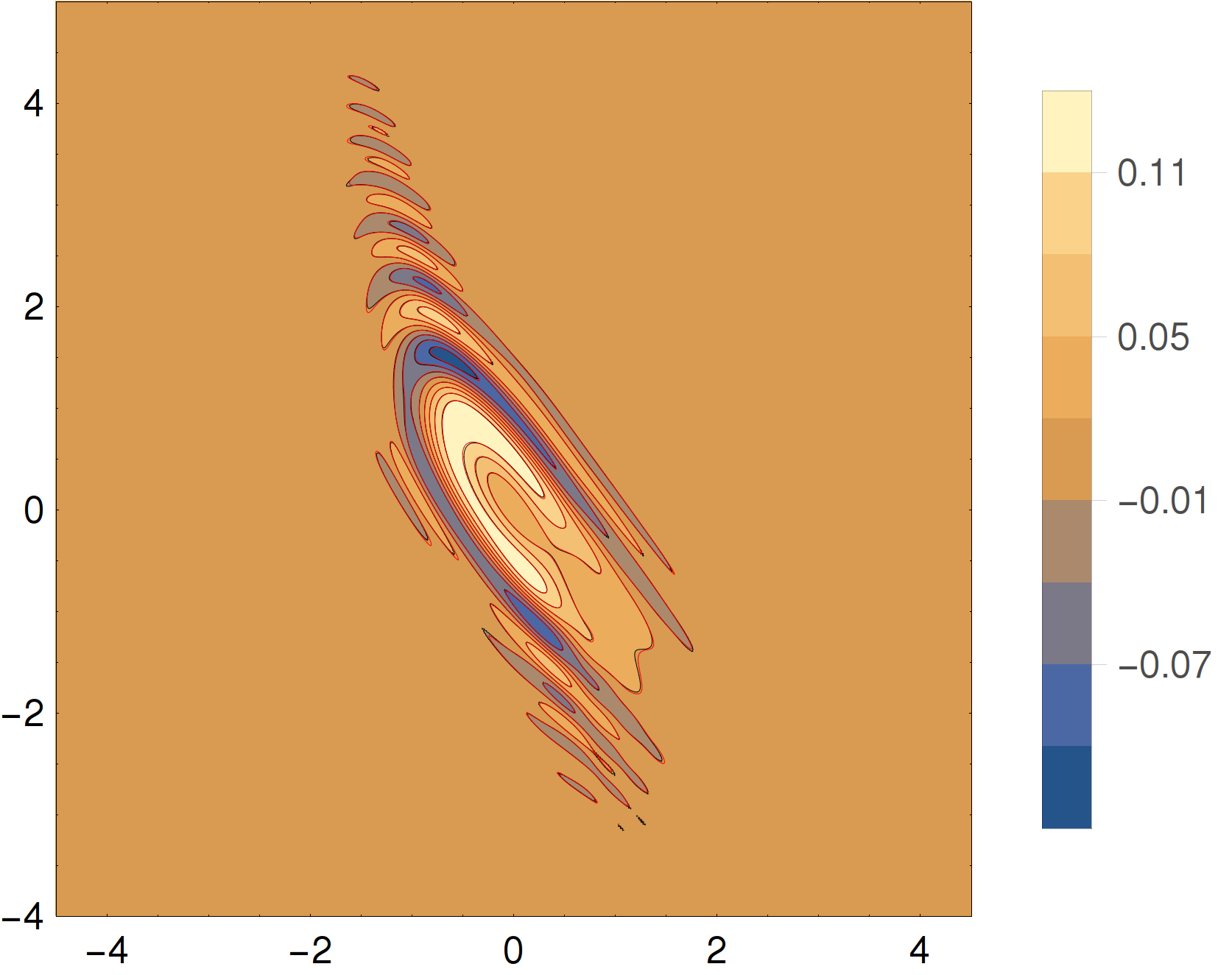
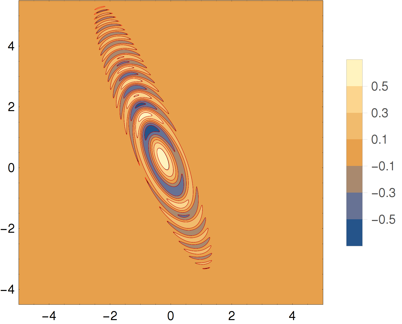
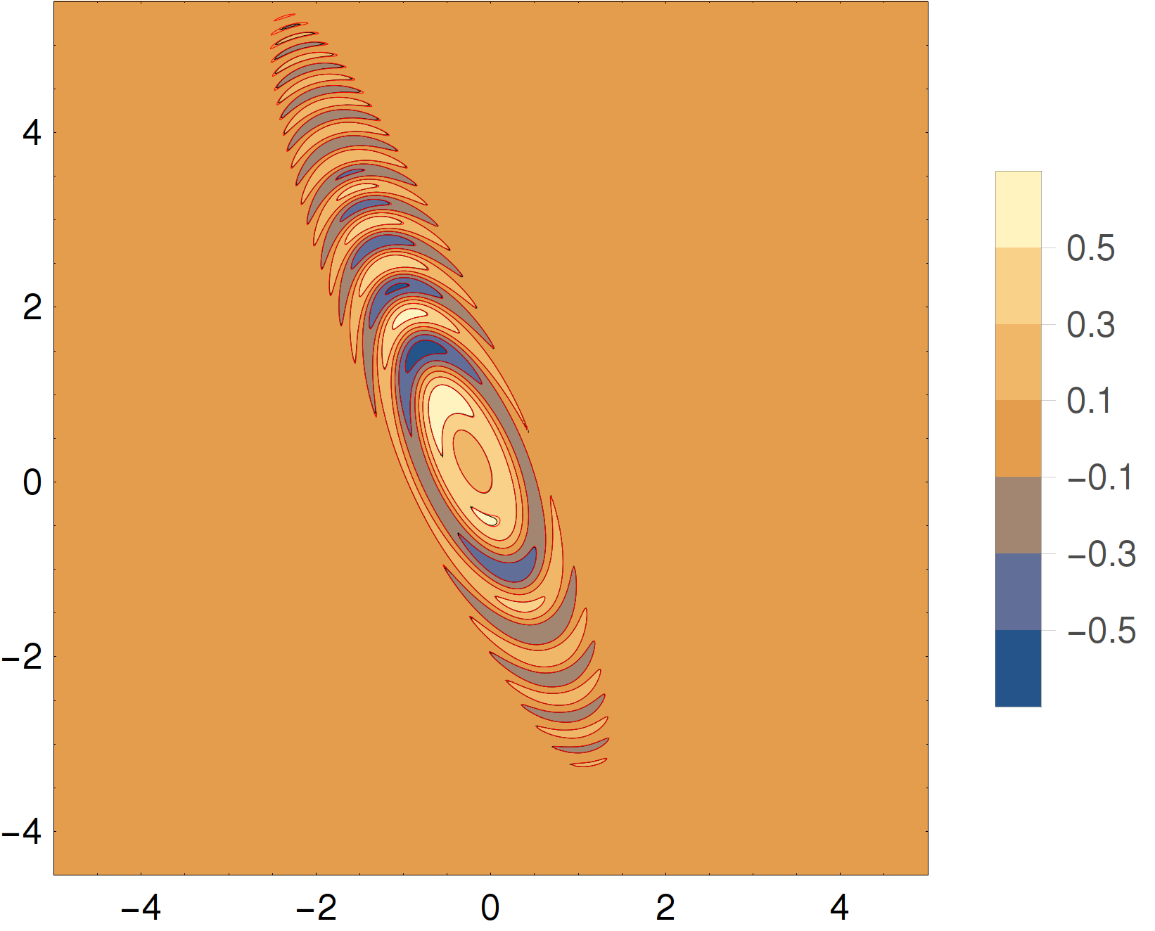
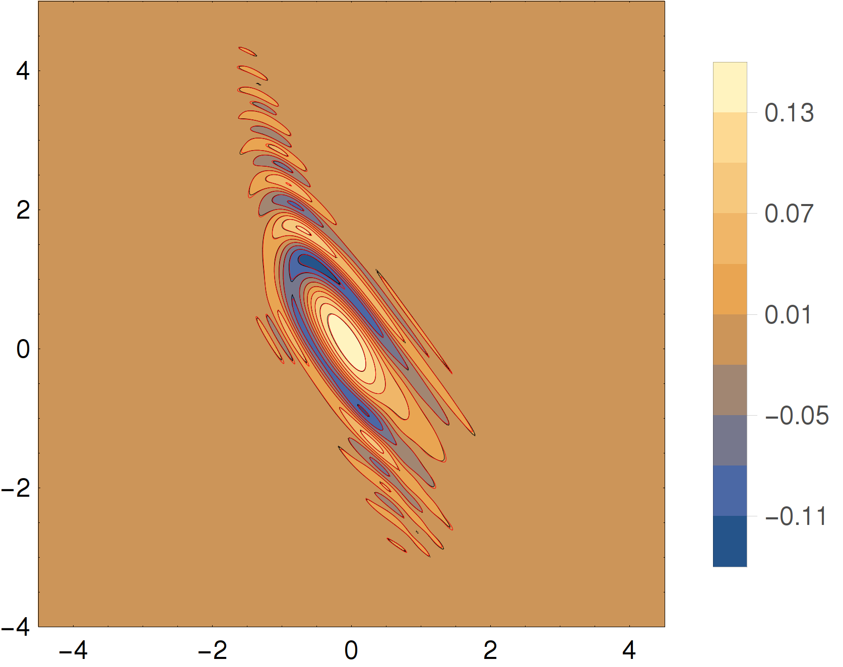
In this example, the coefficients αisubscript𝛼𝑖\alpha_{i} are linear in x𝑥x, βisubscript𝛽𝑖\beta_{i} are quadratic, and γijsubscript𝛾𝑖𝑗\gamma_{ij} are constants. Therefore the O(ϵ12)𝑂superscriptitalic-ϵ12O(\epsilon^{\frac{1}{2}}) residuals in (43) and (46) vanish. Hence the expectation Uiϵ(t,x)superscriptsubscript𝑈𝑖italic-ϵ𝑡𝑥U_{i}^{\epsilon}(t,x) of the surface hopping Gaussian beam method is the exact solution of (56). Since (56) does not have an explicit analytical solution, we solve the system with a finite volume method and the result is used a reference solution. The scheme is third order in both time and space, and the mesh is uniform with grid size Δx1=Δx2=0.02Δsubscript𝑥1Δsubscript𝑥20.02\Delta x_{1}=\Delta x_{2}=0.02. Figure 1 shows the numerical results for ϵ=0.1italic-ϵ0.1\epsilon=0.1 at t=0.5𝑡0.5t=0.5, which are obtained with 100,000 trajectories. The isolines are almost identical to the reference solution, which indicates the feasibility of the surface hopping Gaussian beam method.
Refer to caption
(a) ReU1ϵResuperscriptsubscript𝑈1italic-ϵ\operatorname{Re}U_{1}^{\epsilon}
Refer to caption
(b) ImU1ϵImsuperscriptsubscript𝑈1italic-ϵ\operatorname{Im}U_{1}^{\epsilon}
Refer to caption
(c) ReU2ϵResuperscriptsubscript𝑈2italic-ϵ\operatorname{Re}U_{2}^{\epsilon}
Refer to caption
(d) ImU2ϵImsuperscriptsubscript𝑈2italic-ϵ\operatorname{Im}U_{2}^{\epsilon}
Figure 1. Comparison between the numerical result and the reference solution. The white lines show the contours of the reference solution, and the color shading and black lines (almost covered by the red lines) give the contours of the solution of the surface hopping Gaussian beam method.
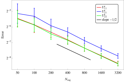
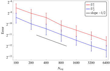
Below we study the convergence of the surface hopping Gaussian beam method with respect to the number of trajectories Ntrajsubscript𝑁trajN_{\mathrm{traj}}. We run the above simulation with 100, 200, 400, 800, 1600, 3200, 6400 trajectories and compute the L2superscript𝐿2L^{2} difference between the numerical solution and the reference solution. The result is plotted in Figure 2, where the case ϵ=0.5italic-ϵ0.5\epsilon=0.5 is also included. The errors in the figure are obtained by averaging the erros of 100 runs in each case, and the error bars show the standard deviations. The figure clearly shows that both the error and its standard deviation decreases as O(Ntraj1/2)𝑂superscriptsubscript𝑁traj12O(N_{\mathrm{traj}}^{-1/2}) when the number of trajectories increases, which agrees with the general property of stochastic numerical methods.
Refer to caption
(a) ϵ=0.1italic-ϵ0.1\epsilon=0.1
Refer to caption
(b) ϵ=0.5italic-ϵ0.5\epsilon=0.5
Figure 2. Log-log plot of the L2superscript𝐿2L^{2} errors for U1ϵsuperscriptsubscript𝑈1italic-ϵU_{1}^{\epsilon} and U2ϵsuperscriptsubscript𝑈2italic-ϵU_{2}^{\epsilon} with different number of trajectories

3.2. An example with nonlinear coefficients

In this section, we consider the system

(60) u1ϵtsin(x1+x2)u1ϵx1cos(x1x2)u1ϵx2=iϵsin(|x|2)u1ϵ|x|2(u1ϵ5u2ϵ),superscriptsubscript𝑢1italic-ϵ𝑡subscript𝑥1subscript𝑥2superscriptsubscript𝑢1italic-ϵsubscript𝑥1subscript𝑥1subscript𝑥2superscriptsubscript𝑢1italic-ϵsubscript𝑥2iitalic-ϵsuperscript𝑥2superscriptsubscript𝑢1italic-ϵsuperscript𝑥2superscriptsubscript𝑢1italic-ϵ5superscriptsubscript𝑢2italic-ϵ\displaystyle\frac{\partial u_{1}^{\epsilon}}{\partial t}-\sin(x_{1}+x_{2})\frac{\partial u_{1}^{\epsilon}}{\partial x_{1}}-\cos(x_{1}-x_{2})\frac{\partial u_{1}^{\epsilon}}{\partial x_{2}}=\frac{\mathrm{i}}{\epsilon}\sin(|x|^{2})u_{1}^{\epsilon}-|x|^{2}(u_{1}^{\epsilon}-5u_{2}^{\epsilon}),
u2ϵtsin(x1x2)u2ϵx1cos(x1+x2)u2ϵx2=iϵcos(|x|2)u2ϵ|x|2(5u1ϵ+12u2ϵ),superscriptsubscript𝑢2italic-ϵ𝑡subscript𝑥1subscript𝑥2superscriptsubscript𝑢2italic-ϵsubscript𝑥1subscript𝑥1subscript𝑥2superscriptsubscript𝑢2italic-ϵsubscript𝑥2iitalic-ϵsuperscript𝑥2superscriptsubscript𝑢2italic-ϵsuperscript𝑥25superscriptsubscript𝑢1italic-ϵ12superscriptsubscript𝑢2italic-ϵ\displaystyle\frac{\partial u_{2}^{\epsilon}}{\partial t}-\sin(x_{1}-x_{2})\frac{\partial u_{2}^{\epsilon}}{\partial x_{1}}-\cos(x_{1}+x_{2})\frac{\partial u_{2}^{\epsilon}}{\partial x_{2}}=\frac{\mathrm{i}}{\epsilon}\cos(|x|^{2})u_{2}^{\epsilon}-|x|^{2}\left(5u_{1}^{\epsilon}+\frac{1}{2}u_{2}^{\epsilon}\right),

with initial conditions

(61) u1ϵ(0,x)=exp(|x|22ϵ),u2ϵ(0,x)=0.formulae-sequencesuperscriptsubscript𝑢1italic-ϵ0𝑥superscript𝑥22italic-ϵsuperscriptsubscript𝑢2italic-ϵ0𝑥0u_{1}^{\epsilon}(0,x)=\exp\left(-\frac{|x|^{2}}{2\epsilon}\right),\qquad u_{2}^{\epsilon}(0,x)=0.

In this example, the coefficients are nonlinear in x𝑥x, and therefore the O(ϵ12)𝑂superscriptitalic-ϵ12O(\epsilon^{\frac{1}{2}}) residuals in (43) and (46) exist, which will lead to some discrepancy between uiϵsuperscriptsubscript𝑢𝑖italic-ϵu_{i}^{\epsilon} and Uiϵsuperscriptsubscript𝑈𝑖italic-ϵU_{i}^{\epsilon}. Here we again use the finite volume solver to provide a reference solution, and the grid size is Δx1=Δx2=0.005Δsubscript𝑥1Δsubscript𝑥20.005\Delta x_{1}=\Delta x_{2}=0.005.

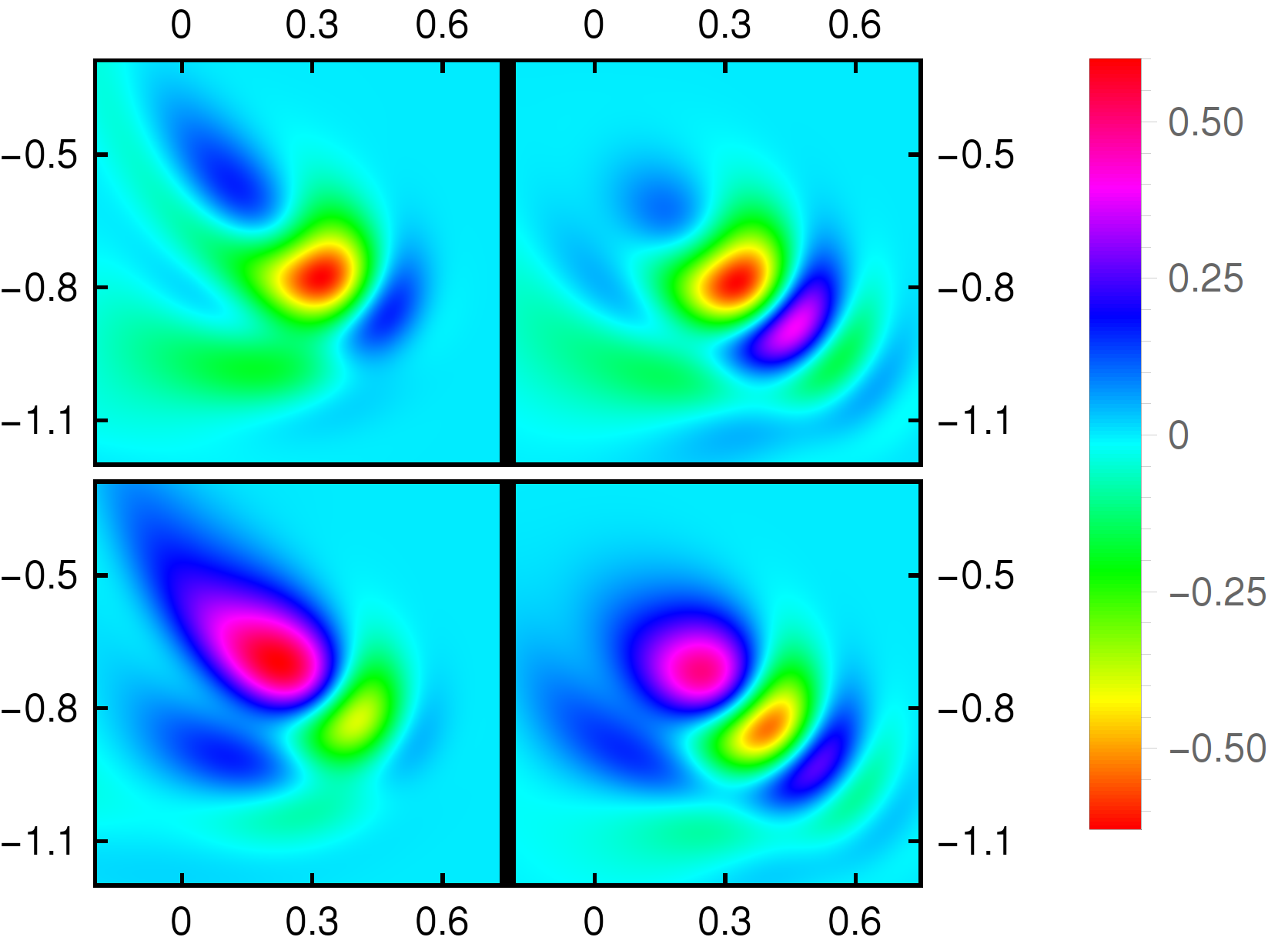
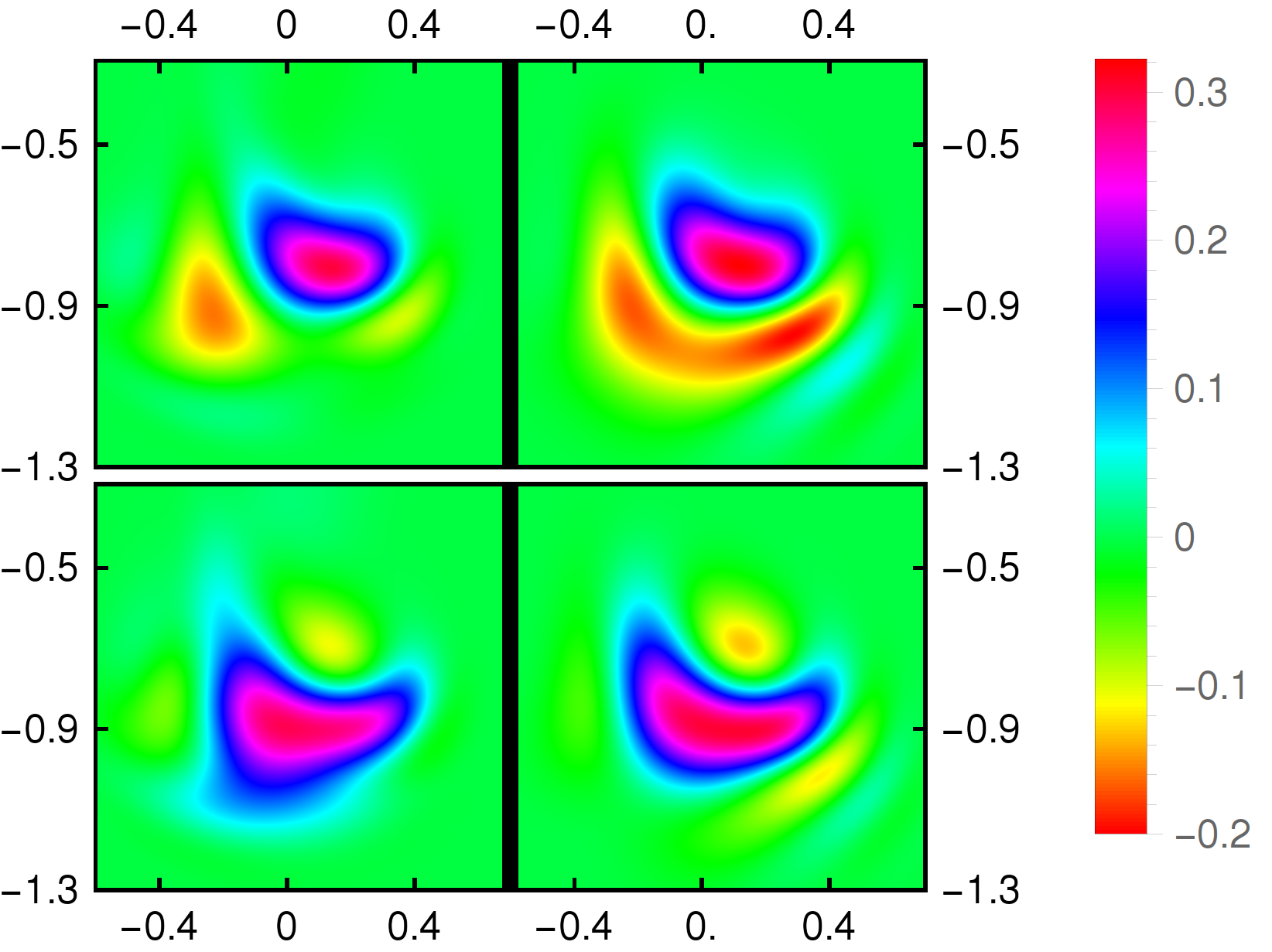
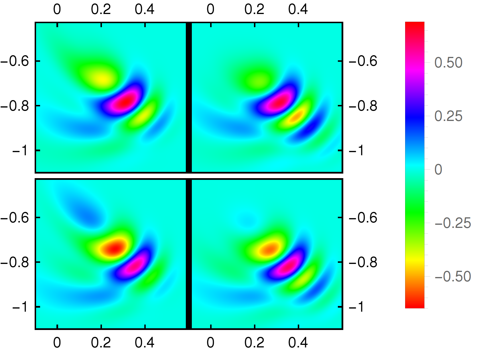
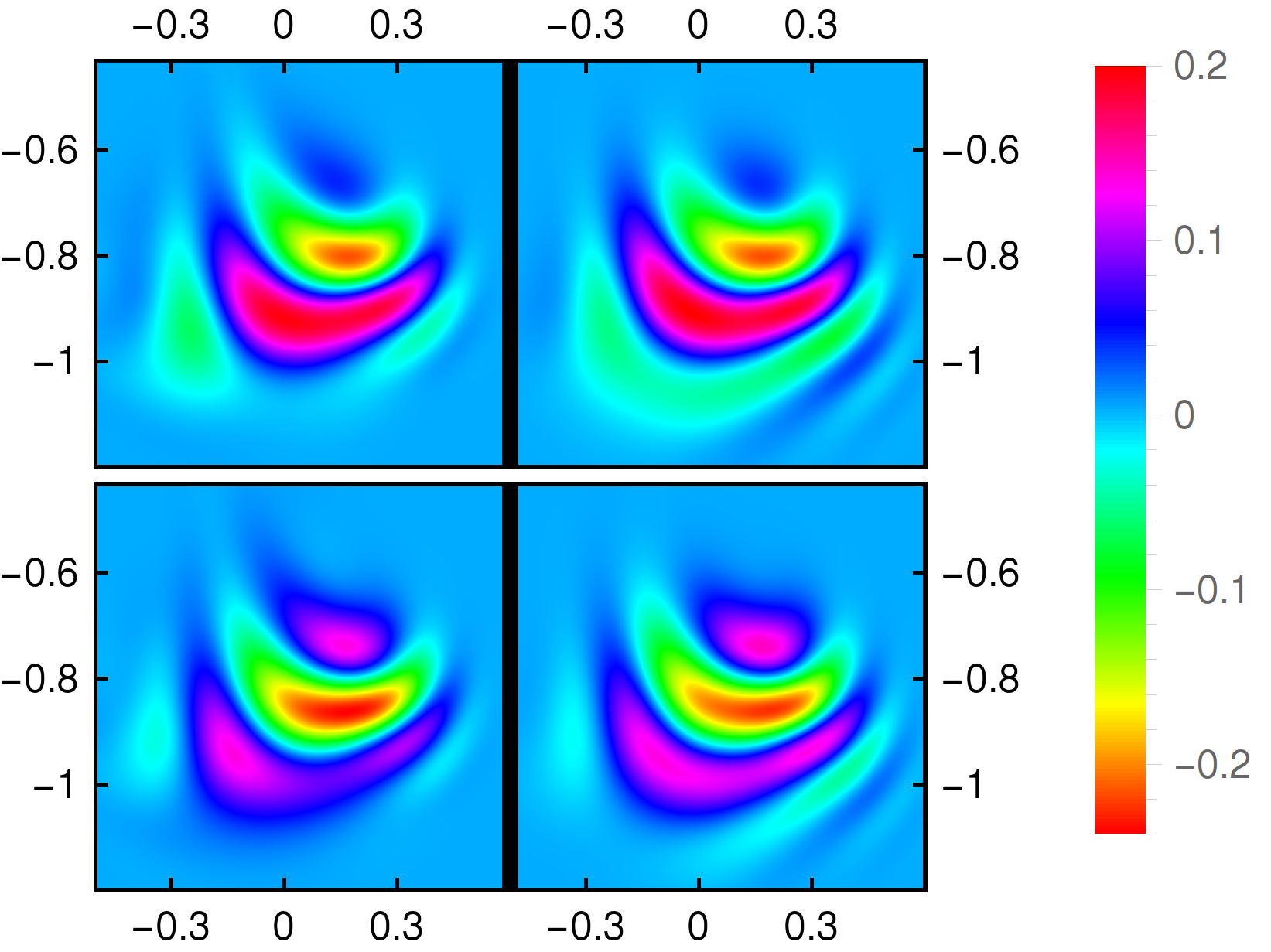
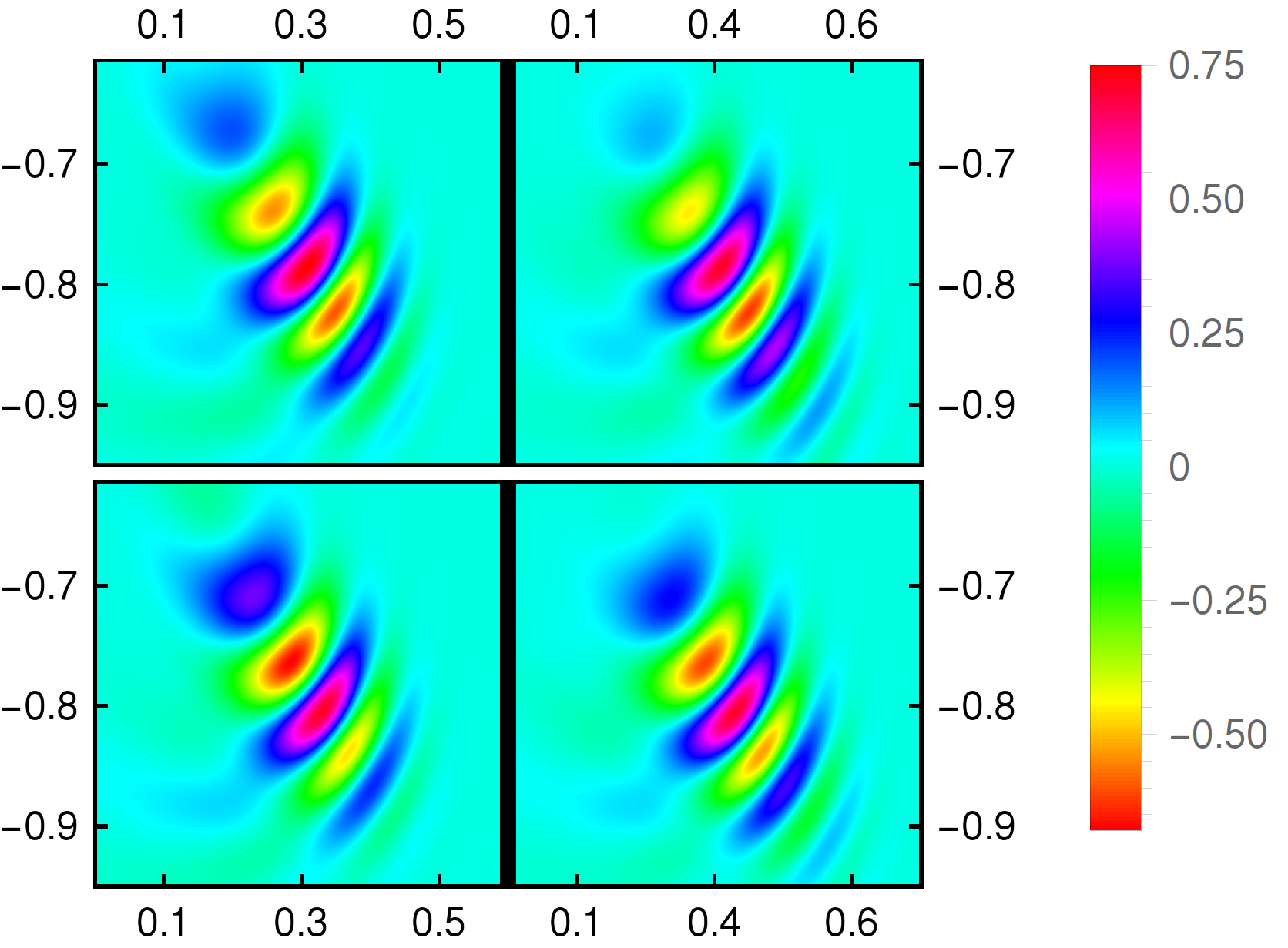
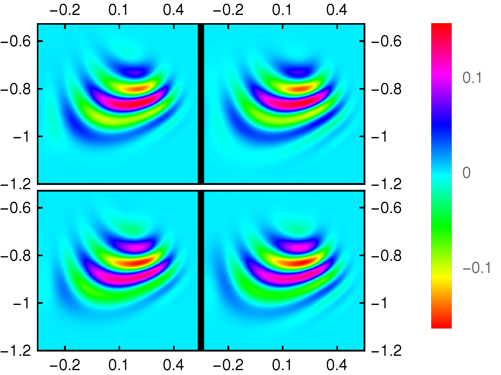
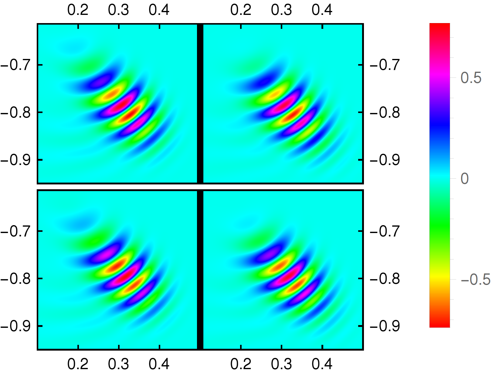
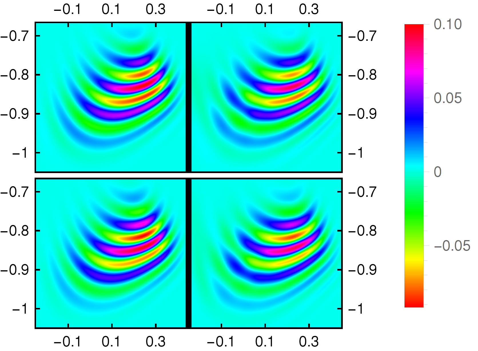
We consider four different values of ϵitalic-ϵ\epsilon. Figure 36 respectively show the results for ϵ=0.08,0.04,0.02,0.01italic-ϵ0.080.040.020.01\epsilon=0.08,0.04,0.02,0.01. All the simulations are performed using 10,000 trajectories. As expected, the solution spreads wider when ϵitalic-ϵ\epsilon increases, and the oscillation gets stronger when ϵitalic-ϵ\epsilon decreases. In all the cases, our method generates reasonable approximate solutoins, while it can still be observed from the figures that better approximation of the reference solution is obtained for smaller ϵitalic-ϵ\epsilon.

Refer to caption
(a) U1ϵsuperscriptsubscript𝑈1italic-ϵU_{1}^{\epsilon} and the reference solution
Refer to caption
(b) U2ϵsuperscriptsubscript𝑈2italic-ϵU_{2}^{\epsilon} and the reference solution
Figure 3. Comparison between the numerical results and the reference solutions with ϵ=0.08italic-ϵ0.08\epsilon=0.08. The upper half of the figure shows the real part of the solution, and the lower half shows the imaginary part. The results of the surface hopping Gaussian beam method are given to the right of the bold black bars, and the left parts are the reference solutions.
Refer to caption
(a) U1ϵsuperscriptsubscript𝑈1italic-ϵU_{1}^{\epsilon} and the reference solution
Refer to caption
(b) U2ϵsuperscriptsubscript𝑈2italic-ϵU_{2}^{\epsilon} and the reference solution
Figure 4. Comparison between the numerical results and the reference solutions with ϵ=0.04italic-ϵ0.04\epsilon=0.04. See Figure 3 for the details.
Refer to caption
(a) U1ϵsuperscriptsubscript𝑈1italic-ϵU_{1}^{\epsilon} and the reference solution
Refer to caption
(b) U2ϵsuperscriptsubscript𝑈2italic-ϵU_{2}^{\epsilon} and the reference solution
Figure 5. Comparison between the numerical results and the reference solutions with ϵ=0.02italic-ϵ0.02\epsilon=0.02. See Figure 3 for the details.
Refer to caption
(a) U1ϵsuperscriptsubscript𝑈1italic-ϵU_{1}^{\epsilon} and the reference solution
Refer to caption
(b) U2ϵsuperscriptsubscript𝑈2italic-ϵU_{2}^{\epsilon} and the reference solution
Figure 6. Comparison between the numerical results and the reference solutions with ϵ=0.01italic-ϵ0.01\epsilon=0.01. See Figure 3 for the details.

3.3. Quantum-classical Liouville equation

In this section, we consider the application of the surface hopping Gaussian beam method to the quantum-classical Liouville equation [24], which describes the composed system with heavy and light particles. The quantum-classical Liouville equation (QCLE) has exactly the form (50), and thus our algorithm can be directly applied. Here we study the two level system as in [4], and write the equations as

(62) u11ϵ(t,r,p)tsuperscriptsubscript𝑢11italic-ϵ𝑡𝑟𝑝𝑡\displaystyle\frac{\partial u_{11}^{\epsilon}(t,r,p)}{\partial t} =pru11ϵ(t,r,p)+rE1(r)pu11ϵ(t,r,p)+[pd21(r)¯]u21ϵ(t,r,p)+[pd21(r)]u21ϵ(t,r,p)¯,absent𝑝subscript𝑟superscriptsubscript𝑢11italic-ϵ𝑡𝑟𝑝subscript𝑟subscript𝐸1𝑟subscript𝑝superscriptsubscript𝑢11italic-ϵ𝑡𝑟𝑝delimited-[]𝑝¯subscript𝑑21𝑟superscriptsubscript𝑢21italic-ϵ𝑡𝑟𝑝delimited-[]𝑝subscript𝑑21𝑟¯superscriptsubscript𝑢21italic-ϵ𝑡𝑟𝑝\displaystyle=-p\cdot\nabla_{r}u_{11}^{\epsilon}(t,r,p)+\nabla_{r}E_{1}(r)\cdot\nabla_{p}u_{11}^{\epsilon}(t,r,p)+[p\cdot\overline{d_{21}(r)}]u_{21}^{\epsilon}(t,r,p)+[p\cdot d_{21}(r)]\overline{u_{21}^{\epsilon}(t,r,p)},
u22ϵ(t,r,p)tsuperscriptsubscript𝑢22italic-ϵ𝑡𝑟𝑝𝑡\displaystyle\frac{\partial u_{22}^{\epsilon}(t,r,p)}{\partial t} =pru22ϵ(t,r,p)+rE2(r)pu11ϵ(t,r,p)[pd21(r)¯]u21ϵ(t,r,p)[pd21(r)]u21ϵ(t,r,p)¯,absent𝑝subscript𝑟superscriptsubscript𝑢22italic-ϵ𝑡𝑟𝑝subscript𝑟subscript𝐸2𝑟subscript𝑝superscriptsubscript𝑢11italic-ϵ𝑡𝑟𝑝delimited-[]𝑝¯subscript𝑑21𝑟superscriptsubscript𝑢21italic-ϵ𝑡𝑟𝑝delimited-[]𝑝subscript𝑑21𝑟¯superscriptsubscript𝑢21italic-ϵ𝑡𝑟𝑝\displaystyle=-p\cdot\nabla_{r}u_{22}^{\epsilon}(t,r,p)+\nabla_{r}E_{2}(r)\cdot\nabla_{p}u_{11}^{\epsilon}(t,r,p)-[p\cdot\overline{d_{21}(r)}]u_{21}^{\epsilon}(t,r,p)-[p\cdot d_{21}(r)]\overline{u_{21}^{\epsilon}(t,r,p)},
u21ϵ(t,r,p)tsuperscriptsubscript𝑢21italic-ϵ𝑡𝑟𝑝𝑡\displaystyle\frac{\partial u_{21}^{\epsilon}(t,r,p)}{\partial t} =iϵ[E2(r)E1(r)]u21ϵ(t,r,p)pru21ϵ(t,r,p)+12r[E1(r)+E2(r)]pu21ϵ(t,r,p)absentiitalic-ϵdelimited-[]subscript𝐸2𝑟subscript𝐸1𝑟superscriptsubscript𝑢21italic-ϵ𝑡𝑟𝑝𝑝subscript𝑟superscriptsubscript𝑢21italic-ϵ𝑡𝑟𝑝12subscript𝑟subscript𝐸1𝑟subscript𝐸2𝑟subscript𝑝superscriptsubscript𝑢21italic-ϵ𝑡𝑟𝑝\displaystyle=-\frac{\mathrm{i}}{\epsilon}[E_{2}(r)-E_{1}(r)]u_{21}^{\epsilon}(t,r,p)-p\cdot\nabla_{r}u_{21}^{\epsilon}(t,r,p)+\frac{1}{2}\nabla_{r}[E_{1}(r)+E_{2}(r)]\cdot\nabla_{p}u_{21}^{\epsilon}(t,r,p)
+[p(d11(r)d22(r))]u21ϵ(t,r,p)[pd21(r)]u11ϵ(t,r,p)+[pd21(r)]u22ϵ(t,r,p),delimited-[]𝑝subscript𝑑11𝑟subscript𝑑22𝑟superscriptsubscript𝑢21italic-ϵ𝑡𝑟𝑝delimited-[]𝑝subscript𝑑21𝑟superscriptsubscript𝑢11italic-ϵ𝑡𝑟𝑝delimited-[]𝑝subscript𝑑21𝑟superscriptsubscript𝑢22italic-ϵ𝑡𝑟𝑝\displaystyle\qquad+[p\cdot(d_{11}(r)-d_{22}(r))]u_{21}^{\epsilon}(t,r,p)-[p\cdot d_{21}(r)]u_{11}^{\epsilon}(t,r,p)+[p\cdot d_{21}(r)]u_{22}^{\epsilon}(t,r,p),

where E1(r),E2(r)subscript𝐸1𝑟subscript𝐸2𝑟E_{1}(r),E_{2}(r)\in\mathbb{R} are adiabatic energy surfaces, rn𝑟superscript𝑛r\in\mathbb{R}^{n} and pn𝑝superscript𝑛p\in\mathbb{R}^{n} stand respectivly for the position and momentum, and dij(r)nsubscript𝑑𝑖𝑗𝑟superscript𝑛d_{ij}(r)\in\mathbb{R}^{n} is used to denote the first-order adiabatic operator. We refer the readers to [24, 4] for the derivation of the above equations, and here we just mention that Ei(r)subscript𝐸𝑖𝑟E_{i}(r) and dij(r)subscript𝑑𝑖𝑗𝑟d_{ij}(r) can be derived from the potential energy matrix acting on the heavy particles V(r)2×2𝑉𝑟superscript22V(r)\in\mathbb{C}^{2\times 2}. Assuming V(r)𝑉𝑟V(r) to be real and symmetric, we have

(63) E1,2(r)=12[V11(r)+V22(r)]±12[V11(r)V22(r)]2+4V122(r),d21(r)=[V11(r)V22(r)]rV12(r)V12(r)r[V11(r)V22(r)][V11(r)V22(r)]2+4V122(r),d11(r)=d22(r)=0.\begin{gathered}E_{1,2}(r)=\frac{1}{2}[V_{11}(r)+V_{22}(r)]\pm\frac{1}{2}\sqrt{[V_{11}(r)-V_{22}(r)]^{2}+4V_{12}^{2}(r)},\\ d_{21}(r)=\frac{[V_{11}(r)-V_{22}(r)]\nabla_{r}V_{12}(r)-V_{12}(r)\nabla_{r}[V_{11}(r)-V_{22}(r)]}{[V_{11}(r)-V_{22}(r)]^{2}+4V_{12}^{2}(r)},\quad d_{11}(r)=d_{22}(r)=0.\end{gathered}

The equations (62) are slightly different from the more conventional QCLE derived in [15, 11]. The system (62) can be considered as the simplified version of the quantum-classical Liouville equations, where a momentum-jump term is absent. The simplification yields a O(ϵ)𝑂italic-ϵO(\epsilon) approximation to the quantum-classical expectation values of physical quantities [24]. We refer the readers to [11, 23, 3] for the comparisons of the two models.

Below we will present two examples to test our method.

3.3.1. Extended coupling with reflection

This example is from one of Tully’s examples in [26]. The number of dimensions n=1𝑛1n=1, and the matrix V(r)𝑉𝑟V(r) is given as

(64) V(r)=(V11(r)V12(r)V12(r)V22(r))=Fδ(r)(120110(arctan(2r)+π2)110(arctan(2r)+π2)120),𝑉𝑟matrixsubscript𝑉11𝑟subscript𝑉12𝑟subscript𝑉12𝑟subscript𝑉22𝑟superscript𝐹𝛿𝑟matrix1201102𝑟𝜋21102𝑟𝜋2120V(r)=\begin{pmatrix}V_{11}(r)&V_{12}(r)\\ V_{12}(r)&V_{22}(r)\end{pmatrix}=F^{\delta}(r)\begin{pmatrix}\frac{1}{20}&\frac{1}{10}\left(\arctan(2r)+\frac{\pi}{2}\right)\\ \frac{1}{10}\left(\arctan(2r)+\frac{\pi}{2}\right)&-\frac{1}{20}\end{pmatrix},

where Fδ(r)=1π(arctan(100r)+π2+δ)superscript𝐹𝛿𝑟1𝜋100𝑟𝜋2𝛿F^{\delta}(r)=\frac{1}{\pi}\left(\arctan(100r)+\frac{\pi}{2}+\delta\right). Here we choose δ=5ϵ𝛿5italic-ϵ\delta=5\epsilon and the initial condition

(65) u11ϵ(0,x)=u12ϵ(0,x)=0,u22ϵ(0,x)=132πϵexp((rr0)2ϵ(pp0)2ϵ),formulae-sequencesuperscriptsubscript𝑢11italic-ϵ0𝑥superscriptsubscript𝑢12italic-ϵ0𝑥0superscriptsubscript𝑢22italic-ϵ0𝑥132𝜋italic-ϵsuperscript𝑟subscript𝑟02italic-ϵsuperscript𝑝subscript𝑝02italic-ϵu_{11}^{\epsilon}(0,x)=u_{12}^{\epsilon}(0,x)=0,\quad u_{22}^{\epsilon}(0,x)=\frac{1}{\sqrt{32\pi}\epsilon}\exp\left(-\frac{(r-r_{0})^{2}}{\epsilon}-\frac{(p-p_{0})^{2}}{\epsilon}\right),

and the initial position and momentum are set to be r0=1.5subscript𝑟01.5r_{0}=-1.5 and p0=1.5subscript𝑝01.5p_{0}=1.5. Three cases ϵ=1/16,1/32,1/64italic-ϵ116132164\epsilon=1/16,1/32,1/64 are considered, and in these cases, the energy surfaces E1,2(r)subscript𝐸12𝑟E_{1,2}(r) and the function d21(r)subscript𝑑21𝑟d_{21}(r) are plotted in Figure 7. From (62), one can find that E1,2(r)subscript𝐸12𝑟E_{1,2}(r) describes the “shape” of the surfaces, and d21(r)subscript𝑑21𝑟d_{21}(r) determines the probability of the surface hopping. In this example, d21(r)subscript𝑑21𝑟d_{21}(r) is indepedent of ϵitalic-ϵ\epsilon. If r>1.5𝑟1.5r>1.5, there are hardly any hops between surfaces.
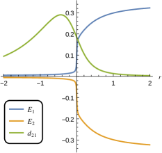
Refer to caption
(a) ϵ=1/16italic-ϵ116\epsilon=1/16
Refer to caption
(b) ϵ=1/32italic-ϵ132\epsilon=1/32
Refer to caption
(c) ϵ=1/64italic-ϵ164\epsilon=1/64
Figure 7. Funtions E1(r)subscript𝐸1𝑟E_{1}(r), E2(r)subscript𝐸2𝑟E_{2}(r) and d21(r)subscript𝑑21𝑟d_{21}(r) for various ϵitalic-ϵ\epsilon

Due to the space limitations, we only plot figures for u11ϵsuperscriptsubscript𝑢11italic-ϵu_{11}^{\epsilon} and u22ϵsuperscriptsubscript𝑢22italic-ϵu_{22}^{\epsilon}. Figure 810 show the comparison with the reference solutions. In all cases, 10,000 trajectories are used and the figures show the solutions at t=2𝑡2t=2. We again observe that better results are obtained for small ϵitalic-ϵ\epsilon. Figure 11 gives a sample of the trajectory in the phase space (r,p)𝑟𝑝(r,p), which is extracted from a test run for ϵ=1/32italic-ϵ132\epsilon=1/32. When r<0𝑟0r<0, both E1(r)subscript𝐸1𝑟E_{1}(r) and E2(r)subscript𝐸2𝑟E_{2}(r) are flat, and thus there is very little change in the momentum p𝑝p. By zooming in, we can still see that the momentum is increasing slowly until the hop occurs. The first hop brings the trajectory onto the u21ϵsuperscriptsubscript𝑢21italic-ϵu_{21}^{\epsilon} surface, where the momentum does not change since E1(r)+E2(r)subscript𝐸1𝑟subscript𝐸2𝑟E_{1}(r)+E_{2}(r) is zero. The second hop almost occurs at the point with highest hopping probability (see Figure 7). Since E1(r)subscript𝐸1𝑟E_{1}(r) is increasing, the momentum starts to drop at this hop. When crossing the point r=0𝑟0r=0, the momentum has the fastest decrease. The last hop occurs near r=0𝑟0r=0, and the momentum again stays as a constant from then on. Later, since r𝑟r keeps increasing, the hopping probability goes lower, no more hops exist in the trajectory.
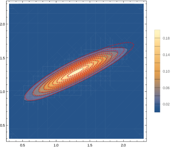
Refer to caption
(a) U11ϵsuperscriptsubscript𝑈11italic-ϵU_{11}^{\epsilon} and the reference solution
Refer to caption
(b) U22ϵsuperscriptsubscript𝑈22italic-ϵU_{22}^{\epsilon} and the reference solution
Figure 8. Comparison between the numerical results (color shading and black contour lines) and the reference solutions (red dotted contour lines) for ϵ=1/16italic-ϵ116\epsilon=1/16.
Refer to caption
(a) U11ϵsuperscriptsubscript𝑈11italic-ϵU_{11}^{\epsilon} and the reference solution
Refer to caption
(b) U22ϵsuperscriptsubscript𝑈22italic-ϵU_{22}^{\epsilon} and the reference solution
Figure 9. Comparison between the numerical results (color shading and black contour lines) and the reference solutions (red dotted contour lines) for ϵ=1/32italic-ϵ132\epsilon=1/32.
Refer to caption
(a) U11ϵsuperscriptsubscript𝑈11italic-ϵU_{11}^{\epsilon} and the reference solution
Refer to caption
(b) U22ϵsuperscriptsubscript𝑈22italic-ϵU_{22}^{\epsilon} and the reference solution
Figure 10. Comparison between the numerical results (color shading and black contour lines) and the reference solutions (red dotted contour lines) for ϵ=1/64italic-ϵ164\epsilon=1/64.
Refer to caption
Figure 11. A sample trajectory with three surface hops

3.3.2. Single crossing

This example is a repetition of the example in [24, 11] with our method. We again consider the one-dimensional case x,p𝑥𝑝x,p\in\mathbb{R}, and the diabatic potential energy matrix is

(66) V(r)=(r21/101/101/r).𝑉𝑟matrixsuperscript𝑟21101101𝑟V(r)=\begin{pmatrix}r^{2}&1/10\\ 1/10&1/r\end{pmatrix}.

Thus we have the potential energy E1,2(r)subscript𝐸12𝑟E_{1,2}(r), effective potential energy 12[E1(r)+E2(r)]12delimited-[]subscript𝐸1𝑟subscript𝐸2𝑟\frac{1}{2}[E_{1}(r)+E_{2}(r)] and the nonadiabatic coupling coefficient d21(r)subscript𝑑21𝑟d_{21}(r) as in Figure 12. The initial value is

(67) u11ϵ(0,r,p)=2πϵexp((rr0)22ϵ2(pp0)2ϵ),u21ϵ(0,r,p)=u22ϵ(0,r,p)=0.formulae-sequencesuperscriptsubscript𝑢11italic-ϵ0𝑟𝑝2𝜋italic-ϵsuperscript𝑟subscript𝑟022italic-ϵ2superscript𝑝subscript𝑝02italic-ϵsuperscriptsubscript𝑢21italic-ϵ0𝑟𝑝superscriptsubscript𝑢22italic-ϵ0𝑟𝑝0u_{11}^{\epsilon}(0,r,p)=\sqrt{\frac{2}{\pi\epsilon}}\exp\left(-\frac{(r-r_{0})^{2}}{2\epsilon}-\frac{2(p-p_{0})^{2}}{\epsilon}\right),\qquad u_{21}^{\epsilon}(0,r,p)=u_{22}^{\epsilon}(0,r,p)=0.

Following the method in [27], we write the initial value as

(68) u11ϵ(0,r,p)=f(r1,p1,r2,p2)A(r1,p1,r2,p2)×exp(r2+p2ϵi[p(r1r2)r(p1p2)]ϵ+i(p1p2)(r1+r2)2ϵ)dr1dp1dr2dp2,\begin{split}u_{11}^{\epsilon}(0,r,p)&=\int_{\mathbb{R}}\int_{\mathbb{R}}\int_{\mathbb{R}}\int_{\mathbb{R}}f(r_{1}^{\prime},p_{1}^{\prime},r_{2}^{\prime},p_{2}^{\prime})A(r_{1}^{\prime},p_{1}^{\prime},r_{2}^{\prime},p_{2}^{\prime})\times\\ &\qquad\qquad\exp\left(-\frac{r^{2}+p^{2}}{\epsilon}-\frac{\mathrm{i}[p(r_{1}^{\prime}-r_{2}^{\prime})-r(p_{1}^{\prime}-p_{2}^{\prime})]}{\epsilon}+\frac{\mathrm{i}(p_{1}^{\prime}-p_{2}^{\prime})(r_{1}^{\prime}+r_{2}^{\prime})}{2\epsilon}\right)\,\mathrm{d}r_{1}^{\prime}\,\mathrm{d}p_{1}^{\prime}\,\mathrm{d}r_{2}^{\prime}\,\mathrm{d}p_{2}^{\prime},\end{split}

where

(69) f(r1,p1,r2,p2)𝑓superscriptsubscript𝑟1superscriptsubscript𝑝1superscriptsubscript𝑟2superscriptsubscript𝑝2\displaystyle f(r_{1}^{\prime},p_{1}^{\prime},r_{2}^{\prime},p_{2}^{\prime}) =118(πϵ)2exp((r1r0)2+(r2r0)26ϵ(p1p0)2+(p2p0)23ϵ),absent118superscript𝜋italic-ϵ2superscriptsuperscriptsubscript𝑟1subscript𝑟02superscriptsuperscriptsubscript𝑟2subscript𝑟026italic-ϵsuperscriptsuperscriptsubscript𝑝1subscript𝑝02superscriptsuperscriptsubscript𝑝2subscript𝑝023italic-ϵ\displaystyle=\frac{1}{18(\pi\epsilon)^{2}}\exp\left(-\frac{(r_{1}^{\prime}-r_{0})^{2}+(r_{2}^{\prime}-r_{0})^{2}}{6\epsilon}-\frac{(p_{1}^{\prime}-p_{0})^{2}+(p_{2}^{\prime}-p_{0})^{2}}{3\epsilon}\right),
(70) A(r1,p1,r2,p2)𝐴superscriptsubscript𝑟1superscriptsubscript𝑝1superscriptsubscript𝑟2superscriptsubscript𝑝2\displaystyle A(r_{1}^{\prime},p_{1}^{\prime},r_{2}^{\prime},p_{2}^{\prime}) =6πϵexp(i(p1p0)(2r1+r0)3ϵi(p2p0)(2r2+r0)3ϵ).absent6𝜋italic-ϵisuperscriptsubscript𝑝1subscript𝑝02superscriptsubscript𝑟1subscript𝑟03italic-ϵisuperscriptsubscript𝑝2subscript𝑝02superscriptsubscript𝑟2subscript𝑟03italic-ϵ\displaystyle=\frac{6}{\sqrt{\pi\epsilon}}\exp\left(\frac{\mathrm{i}(p_{1}^{\prime}-p_{0})(2r_{1}^{\prime}+r_{0})}{3\epsilon}-\frac{\mathrm{i}(p_{2}^{\prime}-p_{0})(2r_{2}^{\prime}+r_{0})}{3\epsilon}\right).

Thus the initial condition can be set by drawing r1superscriptsubscript𝑟1r_{1}^{\prime}, p1superscriptsubscript𝑝1p_{1}^{\prime}, r2superscriptsubscript𝑟2r_{2}^{\prime} and p2superscriptsubscript𝑝2p_{2}^{\prime} from (69).

Refer to caption
(a) Potential energies
Refer to caption
(b) Nonadiabatic coupling
Figure 12. Potential energies and nonadiabatic coupling for the single-crossing example

In our experiment, we follow [24, 11] and choose r0=0.4subscript𝑟00.4r_{0}=0.4, p0=1subscript𝑝01p_{0}=1 and ϵ=0.01italic-ϵ0.01\epsilon=0.01. Figure 13 gives the numerical solution of U11ϵsuperscriptsubscript𝑈11italic-ϵU_{11}^{\epsilon} and U22ϵsuperscriptsubscript𝑈22italic-ϵU_{22}^{\epsilon} using 2,000,000 trajectories at t=0.5𝑡0.5t=0.5. Unlike the last example, the solution no longer has a Gaussian shape after evolution. Our method can still well capture the structure of the solution both qualitatively and quantitatively. Using this as a reference solution, we measure the error of the numerical results for different numbers of trajectories, which are plotted in Figure 14. The errors are again obtained by averaging of 100 runs in each case. The half-order of convergence is still observed.
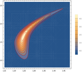
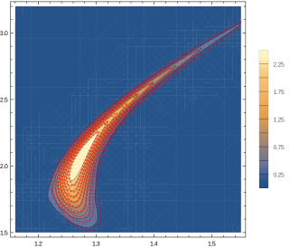
Refer to caption
(a) U11ϵsuperscriptsubscript𝑈11italic-ϵU_{11}^{\epsilon} and the reference solution
Refer to caption
(b) U22ϵsuperscriptsubscript𝑈22italic-ϵU_{22}^{\epsilon} and the reference solution
Figure 13. Comparison between the numerical results (color shading and black contour lines) and the reference solutions (red dotted contour lines) for the single-crossing example.
Refer to caption
Figure 14. L2superscript𝐿2L^{2}-error for different numbers of trajectories

4. Summary

We presented a stochastic numerical method for a type of linear hyperbolic equations with stiff non-coupling source terms and non-stiff coupling source terms. The algorithm combines the Gaussian beam method and the surface hopping method. Similar as [18], this work establishes a surface hopping method based on a solid mathematical foundation, and therefore gives a better understanding of the surface hopping in a general setting. As an algorithm, it is very efficient for initial data with small variance, and works well with the parallelism. As elementary application on the quantum-classical dynamics has been shown, and it can be expected that the algorithm is capable of solving systems with a large number of particles (corresponding to higher spatial dimension), which will be explored in the future.

Appendix A Derivation of the expectation

Here we present the derivation of the formula (24). Define F(t;T1,,TK;i0,i1,,iK)𝐹𝑡subscript𝑇1subscript𝑇𝐾subscript𝑖0subscript𝑖1subscript𝑖𝐾F(t;T_{1},\cdots,T_{K};i_{0},i_{1},\cdots,i_{K}) as the probability that \ell jumps K𝐾K times in [0,t)0𝑡[0,t), and the k𝑘kth jump occurs in [0,Tk]0subscript𝑇𝑘[0,T_{k}] and is from ik1subscript𝑖𝑘1i_{k-1} to iksubscript𝑖𝑘i_{k} (therefore ik1iksubscript𝑖𝑘1subscript𝑖𝑘i_{k-1}\neq i_{k} for every k=1,,K𝑘1𝐾k=1,\cdots,K). Obviously F(t;;)=(J0,t=0)F(t;;)=\mathbb{P}(J_{0,t}=0), and we have

(71) F(t;T1,,TK;i0,,iK)=0min(t,TK)F(tK;T1,,TK1;i0,,iK1)ΩiK1iK(tK)(JtK,t=0)dtK,𝐹𝑡subscript𝑇1subscript𝑇𝐾subscript𝑖0subscript𝑖𝐾superscriptsubscript0𝑡subscript𝑇𝐾𝐹subscript𝑡𝐾subscript𝑇1subscript𝑇𝐾1subscript𝑖0subscript𝑖𝐾1subscriptΩsubscript𝑖𝐾1subscript𝑖𝐾subscript𝑡𝐾subscript𝐽subscript𝑡𝐾𝑡0differential-dsubscript𝑡𝐾F(t;T_{1},\cdots,T_{K};i_{0},\cdots,i_{K})=\int_{0}^{\min(t,T_{K})}F(t_{K};T_{1},\cdots,T_{K-1};i_{0},\cdots,i_{K-1})\Omega_{i_{K-1}i_{K}}(t_{K})\mathbb{P}(J_{t_{K},t}=0)\,\mathrm{d}t_{K},

where tKsubscript𝑡𝐾t_{K} means the time of the K𝐾Kth jump. The recursion relation (71) leads to

(72) F(t;T1,,TK;i0,,iK)=0min(t,TK)0min(tK,Tk1)0min(t2,T1)(k=1KΩik1ik(tk))(k=0K(Jtk,tk+1=0))dt1dtK1dtK,𝐹𝑡subscript𝑇1subscript𝑇𝐾subscript𝑖0subscript𝑖𝐾superscriptsubscript0𝑡subscript𝑇𝐾superscriptsubscript0subscript𝑡𝐾subscript𝑇𝑘1superscriptsubscript0subscript𝑡2subscript𝑇1superscriptsubscriptproduct𝑘1𝐾subscriptΩsubscript𝑖𝑘1subscript𝑖𝑘subscript𝑡𝑘superscriptsubscriptproduct𝑘0𝐾subscript𝐽subscript𝑡𝑘subscript𝑡𝑘10differential-dsubscript𝑡1differential-dsubscript𝑡𝐾1differential-dsubscript𝑡𝐾\begin{split}&F(t;T_{1},\cdots,T_{K};i_{0},\cdots,i_{K})=\\ &\quad\int_{0}^{\min(t,T_{K})}\int_{0}^{\min(t_{K},T_{k-1})}\cdots\int_{0}^{\min(t_{2},T_{1})}\left(\prod_{k=1}^{K}\Omega_{i_{k-1}i_{k}}(t_{k})\right)\left(\prod_{k=0}^{K}\mathbb{P}(J_{t_{k},t_{k+1}}=0)\right)\,\mathrm{d}t_{1}\cdots\,\mathrm{d}t_{K-1}\,\mathrm{d}t_{K},\end{split}

where t0=0subscript𝑡00t_{0}=0 and tK+1=tsubscript𝑡𝐾1𝑡t_{K+1}=t. This formula clearly shows that given t𝑡t and i0,,iKsubscript𝑖0subscript𝑖𝐾i_{0},\cdots,i_{K}, the conditional probability density that the k𝑘kth jump occurs at tksubscript𝑡𝑘t_{k} is

(73) ρ(t1,,tKt;i0,,iK)={0,if tk+1<tk for any k=0,,K,1F(t;i0,,iK)(k=1KΩik1ik(tk))exp(0tΩlsls(s)ds),otherwise,𝜌subscript𝑡1conditionalsubscript𝑡𝐾𝑡subscript𝑖0subscript𝑖𝐾casesformulae-sequence0if subscript𝑡𝑘1subscript𝑡𝑘 for any 𝑘0𝐾otherwise1𝐹𝑡subscript𝑖0subscript𝑖𝐾superscriptsubscriptproduct𝑘1𝐾subscriptΩsubscript𝑖𝑘1subscript𝑖𝑘subscript𝑡𝑘superscriptsubscript0𝑡subscriptΩsubscript𝑙𝑠subscript𝑙𝑠𝑠differential-d𝑠otherwiseotherwise\rho(t_{1},\cdots,t_{K}\mid t;i_{0},\cdots,i_{K})=\begin{cases}0,\quad\text{if }t_{k+1}<t_{k}\text{ for any }k=0,\cdots,K,\\ \displaystyle\frac{1}{F(t;i_{0},\cdots,i_{K})}\left(\prod_{k=1}^{K}\Omega_{i_{k-1}i_{k}}(t_{k})\right)\exp\left(\int_{0}^{t}\Omega_{l_{s}l_{s}}(s)\,\mathrm{d}s\right),\quad\text{otherwise},\end{cases}

where F(t;i0,,iK):=F(t;t,,t;i0,,iK)assign𝐹𝑡subscript𝑖0subscript𝑖𝐾𝐹𝑡𝑡𝑡subscript𝑖0subscript𝑖𝐾F(t;i_{0},\cdots,i_{K}):=F(t;t,\cdots,t;i_{0},\cdots,i_{K}) and lssubscript𝑙𝑠l_{s} is the jump process defined in (25). Consequently, the expectation (19) can be written as

(74) 𝔼[i(;t,x)]=K=0+i1=1i1i0niK=1iKiK1n0+0+i(;t,x)ρ(t1,,tKt;i0,,iK)F(t;i0,,iK)dt1dtK=K=0+i1=1i1i0niK=1iKiK1n0t0tK0t2i(;t,x)(k=1KΩikik1(tk))exp(0tΩlsls(s)ds)dt1dtK1dtK.𝔼delimited-[]subscript𝑖𝑡𝑥superscriptsubscript𝐾0superscriptsubscriptsubscript𝑖11subscript𝑖1subscript𝑖0𝑛superscriptsubscriptsubscript𝑖𝐾1subscript𝑖𝐾subscript𝑖𝐾1𝑛superscriptsubscript0superscriptsubscript0subscript𝑖𝑡𝑥𝜌subscript𝑡1conditionalsubscript𝑡𝐾𝑡subscript𝑖0subscript𝑖𝐾𝐹𝑡subscript𝑖0subscript𝑖𝐾differential-dsubscript𝑡1differential-dsubscript𝑡𝐾superscriptsubscript𝐾0superscriptsubscriptsubscript𝑖11subscript𝑖1subscript𝑖0𝑛superscriptsubscriptsubscript𝑖𝐾1subscript𝑖𝐾subscript𝑖𝐾1𝑛superscriptsubscript0𝑡superscriptsubscript0subscript𝑡𝐾superscriptsubscript0subscript𝑡2subscript𝑖𝑡𝑥superscriptsubscriptproduct𝑘1𝐾subscriptΩsubscript𝑖𝑘subscript𝑖𝑘1subscript𝑡𝑘superscriptsubscript0𝑡subscriptΩsubscript𝑙𝑠subscript𝑙𝑠𝑠differential-d𝑠differential-dsubscript𝑡1differential-dsubscript𝑡𝐾1differential-dsubscript𝑡𝐾\begin{split}&\mathbb{E}[\mathcal{F}_{i}(\ell;t,x)]\\ ={}&\sum_{K=0}^{+\infty}\sum_{\begin{subarray}{c}i_{1}=1\\ i_{1}\neq i_{0}\end{subarray}}^{n}\cdots\sum_{\begin{subarray}{c}i_{K}=1\\ i_{K}\neq i_{K-1}\end{subarray}}^{n}\int_{0}^{+\infty}\!\!\cdots\!\int_{0}^{+\infty}\mathcal{F}_{i}(\ell;t,x)\rho(t_{1},\cdots,t_{K}\mid t;i_{0},\cdots,i_{K})F(t;i_{0},\cdots,i_{K})\,\mathrm{d}t_{1}\cdots\,\mathrm{d}t_{K}\\ ={}&\sum_{K=0}^{+\infty}\sum_{\begin{subarray}{c}i_{1}=1\\ i_{1}\neq i_{0}\end{subarray}}^{n}\cdots\sum_{\begin{subarray}{c}i_{K}=1\\ i_{K}\neq i_{K-1}\end{subarray}}^{n}\int_{0}^{t}\!\!\int_{0}^{t_{K}}\!\!\cdots\!\int_{0}^{t_{2}}\mathcal{F}_{i}(\ell;t,x)\left(\prod_{k=1}^{K}\Omega_{i_{k}i_{k-1}}(t_{k})\right)\exp\left(\int_{0}^{t}\Omega_{l_{s}l_{s}}(s)\,\mathrm{d}s\right)\,\mathrm{d}t_{1}\cdots\,\mathrm{d}t_{K-1}\,\mathrm{d}t_{K}.\end{split}

Here \ell is the jump process defined by (25). This result is identical to (24).

References

  • [1] G. Ariel, B. Engquist, N. Tanushev, and R. Tsai, Gaussian beam decomposition of high frequency wave fields using expectation-maximization, J. Comput. Phys. 230 (2011), no. 6, 2303–2321.
  • [2] M. Barbatti, Nonadiabatic dynamics with trajectory surface hopping method, WIREs comput. Mol. Sci. 1 (2011), no. 4, 620–633.
  • [3] Z. Cai and J. Lu, In preparation.
  • [4] L. Chai, S. Jin, Q. Li, and O. Morandi, A multi-band semiclassical model for surface hopping quantum dynamics, Multiscale Model. Simul. 13 (2015), no. 1, 205–230.
  • [5] N. Crouseilles, S. Jin, and M. Lemou, Nonlinear geometric optics method based multi-scale mumerical schemes for highly-oscillatory transport equations, arXiv:1605.09676 (2016).
  • [6] L. Dieci and T. Eirola, Positive definiteness in the numerical solution of Riccati differential equations, Numerische Mathematik 67 (1994), no. 3, 303–313.
  • [7] W. Dou, A. Nitzan, and J. E. Subotnik, Frictional effects near a metal surface, J. Chem. Phys. 143 (2015), no. 5, 054103.
  • [8] F. Elste, G. Weick, C. Timm, and F. von Oppen, Current-induced conformational switching in single-molecule junctions, Appl. Phys. A 93 (2008), no. 2, 345–354.
  • [9] G. A. Hagedorn, Raising and lowering operators for semiclassical wave packets, Comm. Pure Appl. Math. 50 (1997), no. 4, 323–379.
  • [10] E. J. Heller, Frozen Gaussians: A very simple semiclassical approximation, J. Chem. Phys. 75 (1981), no. 6, 2923–2931.
  • [11] I. Horenko, C. Salzmann, B. Schmidt, and C. Schütte, Quantum-classical Liouville approach to molecular dynamics: Surface hopping Gaussian phase-space packets, J. Chem. Phys. 117 (2002), no. 24, 11075–11088.
  • [12] I. Horenko, B. Schmidt, and C. Schütte, Multidimensional classical Liouville dynamics with quantum initial conditions, J. Chem. Phys. 117 (2002), no. 10, 4643–4650.
  • [13] W. Hundsdorfer and J. Verwer, Numerical solution of time-dependent advection-diffusion-reaction equations, Computational Mathematics, vol. 33, Springer, 2003.
  • [14] R. Kapral, Surface hopping from the perspective of quantum-classical Liouville dynamics, Chem. Phys. 481 (2016), 77–83.
  • [15] R. Kapral and G. Ciccotti, Mixed quantum-classical dynamics, J. Chem. Phys. 110 (1999), no. 18, 8919–8929.
  • [16] A. Kelly and T. E. Markland, Efficient and accurate surface hopping for long time nonadiabatic quantum dynamics, J. Chem. Phys. 139 (2013), no. 1, 014104.
  • [17] D. Mac Kernan, G. Ciccotti, and R. Kapral, Trotter-based simulation of quantum-classical dynamics, J. Phys. Chem. B 112 (2008), no. 2, 424–432.
  • [18] J. Lu and Z. Zhou, Frozen Gaussian approximation with surface hopping for mixed quantum-classical dynamics: A mathematical justification of fewest switches surface hopping algorithms, http://arxiv.org/abs/1602.06459.
  • [19] J. Ma, D. Hsu, and J. E. Straub, Approximate solution of the classical Liouville equation using gaussian phase packet dynamics: Application to enhanced equilibrium averaging and global optimization, J. Chem. Phys. 99 (1993), no. 5, 4024–4035.
  • [20] D. MacKernan, R. Kapral, and G. Ciccotti, Sequential short-time propagation of quantum-classical dynamics, J. Phys.: Condens. Matter 14 (2002), no. 40, 9069–9076.
  • [21] J. Qian and L. Ying, Fast multiscale Gaussian wavepacket transforms and multiscale Gaussian beams for the wave equation, Multiscale Model. Simul. 8 (2010), no. 5, 1803–1837.
  • [22] J. Ralston, Gaussian beams and the propagation of singularities, Studies in Partial Differential Equations, Studies in mathematics, vol. 23, Mathematical Association of America, 1982, pp. 206–248.
  • [23] I. G. Ryabinkin, C.-Y. Hsieh, R. Kapral, and A. F. Izmaylov, Analysis of geometric phase effects in the quantum-classical Liouville formalism, J. Chem. Phys. 140 (2014), no. 8, 084104.
  • [24] C. Schütte, Partial Wigner transforms and the quantum-classical Liouville equation, Tech. Report SC-99-10, Konrad-Zuse-Center, 1999.
  • [25] N. M. Tanushev, Superpositions and higher order Gaussian beams, Commun. Math. Sci. 6 (2008), no. 2, 449–475.
  • [26] J. C. Tully, Molecular dynamics with electronic transitions, J. Chem. Phys. 93 (1990), no. 2, 1061–1071.
  • [27] D. Yin, M. Tang, and S. Jin, The Gaussian beam method for the Wigner equation with discontinuous potentials, Inv. Prob. Imag. 7 (2013), no. 3, 1051–1074.