Combined analysis of semileptonic B𝐵B decays to D𝐷D and Dsuperscript𝐷D^{*}: R(D())𝑅superscript𝐷R(D^{(*)}), |Vcb|subscript𝑉𝑐𝑏|V_{cb}|, and new physics

Florian U. Bernlochner Physikalisches Institut der Rheinischen Friedrich-Wilhelms-Universität Bonn, 53115 Bonn, Germany    Zoltan Ligeti Ernest Orlando Lawrence Berkeley National Laboratory, University of California, Berkeley, CA 94720, USA    Michele Papucci Ernest Orlando Lawrence Berkeley National Laboratory, University of California, Berkeley, CA 94720, USA    Dean J. Robinson Physics Department, University of Cincinnati, Cincinnati OH 45221, USA
Abstract

The measured B¯D()lν¯¯𝐵superscript𝐷𝑙¯𝜈\bar{B}\to D^{(*)}l\bar{\nu} decay rates for light leptons (l=e,μ𝑙𝑒𝜇l=e,\mu) constrain all B¯D()¯𝐵superscript𝐷\bar{B}\to D^{(*)} semileptonic form factors, by including both the leading and 𝒪(ΛQCD/mc,b)𝒪subscriptΛQCDsubscript𝑚𝑐𝑏{\cal O}(\Lambda_{\text{QCD}}/m_{c,b}) subleading Isgur-Wise functions in the heavy quark effective theory. We perform a novel combined fit to the B¯D()lν¯¯𝐵superscript𝐷𝑙¯𝜈\bar{B}\to D^{(*)}l\bar{\nu} decay distributions to predict the B¯D()τν¯¯𝐵superscript𝐷𝜏¯𝜈\bar{B}\to D^{(*)}\tau\bar{\nu} rates and determine the CKM matrix element |Vcb|subscript𝑉𝑐𝑏|V_{cb}|. Most theoretical and experimental papers have neglected uncertainties in the predictions for form factor ratios at order ΛQCD/mc,bsubscriptΛQCDsubscript𝑚𝑐𝑏\Lambda_{\text{QCD}}/m_{c,b}, which we include. We also calculate 𝒪(ΛQCD/mc,b)𝒪subscriptΛQCDsubscript𝑚𝑐𝑏{\cal O}(\Lambda_{\text{QCD}}/m_{c,b}) and 𝒪(αs)𝒪subscript𝛼𝑠{\cal O}(\alpha_{s}) contributions to semileptonic B¯D()ν¯¯𝐵superscript𝐷¯𝜈\bar{B}\to D^{(*)}\ell\bar{\nu} decays for all possible bc𝑏𝑐b\to c currents. This result has not been available for the tensor current form factors, and for two of those, which are 𝒪(ΛQCD/mc,b)𝒪subscriptΛQCDsubscript𝑚𝑐𝑏{\cal O}(\Lambda_{\text{QCD}}/m_{c,b}), the corrections are of the same order as approximations used in the literature. These results allow us to determine with improved precision how new physics may affect the B¯D()τν¯¯𝐵superscript𝐷𝜏¯𝜈\bar{B}\to D^{(*)}\tau\bar{\nu} rates. Our predictions can be systematically improved with more data; they need not rely on lattice QCD results, although these can be incorporated.

I introduction

Heavy quark symmetry Isgur and Wise (1989, 1990) plays an essential role in understanding exclusive semileptonic bcν¯𝑏𝑐¯𝜈b\to c\ell\bar{\nu} mediated transitions, by providing relations between hadronic form factors. At leading order in ΛQCD/mc,bsubscriptΛQCDsubscript𝑚𝑐𝑏\Lambda_{\rm QCD}/m_{c,b}, the symmetry also determines the absolute normalization of form factors at the “zero recoil” point, vB=vD()subscript𝑣𝐵subscript𝑣superscript𝐷v_{B}=v_{D^{(*)}}, corresponding to maximal invariant mass, q2superscript𝑞2q^{2}, of the outgoing lepton pair. Incorporating small corrections to the symmetry limit permits a (hadronic) model-independent determination of |Vcb|subscript𝑉𝑐𝑏|V_{cb}| from exclusive decays. Recently, the Babar Lees et al. (2012, 2013), Belle Huschle et al. (2015); Abdesselam et al. (2016a, b), and LHCb Aaij et al. (2015) measurements of the |Vcb|subscript𝑉𝑐𝑏|V_{cb}|-independent ratios

R(D())=Γ(B¯D()τν¯)Γ(B¯D()lν¯),l=μ,e,formulae-sequence𝑅superscript𝐷Γ¯𝐵superscript𝐷𝜏¯𝜈Γ¯𝐵superscript𝐷𝑙¯𝜈𝑙𝜇𝑒R(D^{(*)})=\frac{\Gamma({\,\overline{\!B}{}\to D^{(*)}\tau\bar{\nu}})}{\Gamma({\,\overline{\!B}{}\to D^{(*)}l\bar{\nu}})}\,,\qquad l=\mu,\,e\,, (1)

renewed interest in these decays. The world average of R(D)𝑅𝐷R(D) and R(D)𝑅superscript𝐷R(D^{*}) is in tension with the SM expectation at the 4σ4𝜎4\sigma level Amhis et al. (2016). This is intriguing as it occurs in a tree-level SM process, while most new physics (NP) explanations require new states at or below one TeV Freytsis et al. (2015).

Besides the search for new physics, understanding bcν¯𝑏𝑐¯𝜈b\to c\ell\bar{\nu} mediated semileptonic decays as precisely as possible is also important for future improvements of the determinations of the CKM elements |Vcb|subscript𝑉𝑐𝑏|V_{cb}| and |Vub|subscript𝑉𝑢𝑏|V_{ub}|, both from exclusive and inclusive B𝐵B decays, which exhibit some tensions Amhis et al. (2016). Depending on the particular measurement, some decay modes contribute to the signals, some to the backgrounds. Future progress is essential for increasing the scale of new physics probed by the Belle II and LHCb experiments Charles et al. (2014).

The main uncertainty in predicting R(D())𝑅superscript𝐷R(D^{(*)}) comes from the fact that the B¯D()τν¯¯𝐵superscript𝐷𝜏¯𝜈{\,\overline{\!B}{}\to D^{(*)}\tau\bar{\nu}} decay rates depend on certain form factors, that only give ml2/mB2superscriptsubscript𝑚𝑙2superscriptsubscript𝑚𝐵2m_{l}^{2}/m_{B}^{2} suppressed contributions to the differential rates for the precisely measured light lepton channels. Using heavy quark effective theory (HQET), however, all B¯D()¯𝐵superscript𝐷\,\overline{\!B}{}\to D^{(*)} form factors are described by a single Isgur-Wise function in the mc,bΛQCDmuch-greater-thansubscript𝑚𝑐𝑏subscriptΛQCDm_{c,b}\gg\Lambda_{\rm QCD} limit. At order ΛQCD/mc,bsubscriptΛQCDsubscript𝑚𝑐𝑏\Lambda_{\rm QCD}/m_{c,b}, only three additional functions of q2superscript𝑞2q^{2} are needed to parametrize all form factors.

We perform the first combined fit to B¯D()lν¯¯𝐵superscript𝐷𝑙¯𝜈{\,\overline{\!B}{}\to D^{(*)}l\bar{\nu}} differential rates and angular distributions, including 𝒪(ΛQCD/mc,b,αs)𝒪subscriptΛQCDsubscript𝑚𝑐𝑏subscript𝛼𝑠\mathcal{O}(\Lambda_{\rm QCD}/{m_{c,b}},\,\alpha_{s}) terms in HQET, to constrain both the leading and three subleading Isgur-Wise functions. This fit constrains all form factors, up to higher order corrections, with uncertainties suppressed by 𝒪(ΛQCD2/mc,b2,αsΛQCD/mc,b,αs2)𝒪superscriptsubscriptΛQCD2subscriptsuperscript𝑚2𝑐𝑏subscript𝛼𝑠subscriptΛQCDsubscript𝑚𝑐𝑏superscriptsubscript𝛼𝑠2\mathcal{O}(\Lambda_{\rm QCD}^{2}/m^{2}_{c,b}\,,\,\alpha_{s}\Lambda_{\rm QCD}/m_{c,b}\,,\,\alpha_{s}^{2}). We extract |Vcb|subscript𝑉𝑐𝑏|V_{cb}| and form factor ratios under various fit scenarios, that include or omit lattice QCD and/or QCD sum rule inputs, and which provide checks of previously untested theory assumptions or results. Most prior theoretical and experimental studies neglected HQET relations for the form factors at order ΛQCD/mc,bsubscriptΛQCDsubscript𝑚𝑐𝑏\Lambda_{\rm QCD}/m_{c,b} or the correlations of the uncertainties in the deviations from the heavy quark limit. Our fits fully incorporate these. These fits also allow precise predictions of the B¯D()τν¯¯𝐵superscript𝐷𝜏¯𝜈{\,\overline{\!B}{}\to D^{(*)}\tau\bar{\nu}} rates and R(D())𝑅superscript𝐷R(D^{(*)}). Our predictions can be systematically improved with more B¯D()lν¯¯𝐵superscript𝐷𝑙¯𝜈{\,\overline{\!B}{}\to D^{(*)}l\bar{\nu}} data, and need not rely on lattice QCD results. A similar approach to analyze B¯Dlν¯¯𝐵superscript𝐷absent𝑙¯𝜈\,\overline{\!B}{}\to D^{**}l\bar{\nu} decays was recently carried out in Ref. Bernlochner and Ligeti (2017).

We also compute, for all possible bc𝑏𝑐b\to c currents, the 𝒪(ΛQCD/mc,b)𝒪subscriptΛQCDsubscript𝑚𝑐𝑏\mathcal{O}(\Lambda_{\rm QCD}/m_{c,b}) and 𝒪(αs)𝒪subscript𝛼𝑠\mathcal{O}(\alpha_{s}) contributions to the form factors. While the 𝒪(ΛQCD/mc,b)𝒪subscriptΛQCDsubscript𝑚𝑐𝑏\mathcal{O}(\Lambda_{\rm QCD}/m_{c,b}) corrections to the vector and axial-vector matrix elements have been known for over 25 years Luke (1990); Neubert and Rieckert (1992), the corrections for the tensor current form factors are not explicitly available in past literature. Two of these form factors vanish in the heavy quark limit, and receive unsuppressed corrections to the partial results, also of order ΛQCD/mc,bsubscriptΛQCDsubscript𝑚𝑐𝑏\Lambda_{\rm QCD}/m_{c,b}, used previously in the literature.

Section II contains the HQET calculations of the form factors, including order ΛQCD/mc,bsubscriptΛQCDsubscript𝑚𝑐𝑏\Lambda_{\rm QCD}/m_{c,b} and αssubscript𝛼𝑠\alpha_{s} contributions, corresponding expressions for form factor ratios, and some details of our numerical evaluations in the 1S1𝑆1S scheme to avoid known bad behaviors in the perturbation expansions. In Section III we review analyticity constraints on the form factors, parametrizations of the Isgur-Wise functions, and develop several fit scenarios consistent with HQET, which we apply to the data. The results for |Vcb|subscript𝑉𝑐𝑏|V_{cb}|, form factor ratios, and R(D())𝑅superscript𝐷R(D^{(*)}) are discussed. Section IV concludes.

II Elements of HQET

II.1 Matrix elements to order ΛQCD/mc,bsubscriptΛQCDsubscript𝑚𝑐𝑏\Lambda_{\rm QCD}/m_{c,b} and αssubscript𝛼𝑠\alpha_{s}

We are concerned with matrix elements D()|OΓ|B¯quantum-operator-productsuperscript𝐷subscript𝑂Γ¯𝐵\langle D^{(*)}|\,O_{\Gamma}\,|\,\overline{\!B}{}\rangle, where a full operator basis is

OS=c¯b,OP=c¯γ5b,OV=c¯γμb,OA=c¯γμγ5b,OT=c¯σμνb,formulae-sequencesubscript𝑂𝑆¯𝑐𝑏formulae-sequencesubscript𝑂𝑃¯𝑐superscript𝛾5𝑏formulae-sequencesubscript𝑂𝑉¯𝑐superscript𝛾𝜇𝑏formulae-sequencesubscript𝑂𝐴¯𝑐superscript𝛾𝜇superscript𝛾5𝑏subscript𝑂𝑇¯𝑐superscript𝜎𝜇𝜈𝑏O_{S}=\bar{c}\,b\,,\qquad O_{P}=\bar{c}\,\gamma^{5}\,b\,,\qquad O_{V}=\bar{c}\,\gamma^{\mu}\,b\,,\qquad O_{A}=\bar{c}\,\gamma^{\mu}\gamma^{5}\,b\,,\qquad O_{T}=\bar{c}\,\sigma^{\mu\nu}\,b\,, (2)

with σμν(i/2)[γμ,γν]superscript𝜎𝜇𝜈𝑖2superscript𝛾𝜇superscript𝛾𝜈\sigma^{\mu\nu}\equiv(i/2)[\gamma^{\mu},\gamma^{\nu}]. (The sign convention is fixed by σμνγ5(i/2)ϵμνρσσρσsuperscript𝜎𝜇𝜈superscript𝛾5𝑖2superscriptitalic-ϵ𝜇𝜈𝜌𝜎subscript𝜎𝜌𝜎\sigma^{\mu\nu}\gamma^{5}\equiv-(i/2)\epsilon^{\mu\nu\rho\sigma}\sigma_{\rho\sigma}, which implies Tr[γμγνγσγργ5]=+4iϵμνρσTrdelimited-[]superscript𝛾𝜇superscript𝛾𝜈superscript𝛾𝜎superscript𝛾𝜌superscript𝛾54𝑖superscriptitalic-ϵ𝜇𝜈𝜌𝜎\text{Tr}[\gamma^{\mu}\gamma^{\nu}\gamma^{\sigma}\gamma^{\rho}\gamma^{5}]=+4i\epsilon^{\mu\nu\rho\sigma}.) The construction of the HQET expansion to order 𝒪(ΛQCD/mc,b)𝒪subscriptΛQCDsubscript𝑚𝑐𝑏\mathcal{O}(\Lambda_{\rm QCD}/m_{c,b}) and 𝒪(αs)𝒪subscript𝛼𝑠\mathcal{O}(\alpha_{s}) was developed in the early ’90s Manohar and Wise (2000); Neubert (1994); we summarize here the central elements to establish our conventions.

The HQET allows model independent parametrization of the spectroscopy of heavy mesons and some hadronic matrix elements between them. The ground state heavy quark spin symmetry doublet pseudoscalar (P𝑃P) and vector (V𝑉V) mesons correspond to the light degrees of freedom (the “brown muck”) in a spin-1212\frac{1}{2} state combined with the heavy quark spin. They form two states with angular momentum JV,P=12±12subscript𝐽𝑉𝑃plus-or-minus1212J_{V,P}=\frac{1}{2}\pm\frac{1}{2}. Their masses can be expressed as

mV,P=mQ+Λ¯λ12mQ±(2JP,V+1)λ22mQ+,subscript𝑚𝑉𝑃plus-or-minussubscript𝑚𝑄¯Λsubscript𝜆12subscript𝑚𝑄2subscript𝐽𝑃𝑉1subscript𝜆22subscript𝑚𝑄m_{V,P}=m_{Q}+\bar{\Lambda}-\frac{\lambda_{1}}{2m_{Q}}\pm\frac{(2J_{P,V}+1)\lambda_{2}}{2m_{Q}}+\ldots\,, (3)

where mQsubscript𝑚𝑄m_{Q} is the heavy quark mass parameter of HQET, Λ¯=𝒪(ΛQCD)¯Λ𝒪subscriptΛQCD\bar{\Lambda}={\cal O}(\Lambda_{\rm QCD}), λ1,2=𝒪(ΛQCD2)subscript𝜆12𝒪superscriptsubscriptΛQCD2\lambda_{1,2}={\cal O}(\Lambda_{\rm QCD}^{2}), etc. To evaluate matrix elements relevant for semileptonic decays, it is simplest to use the trace formalism Falk et al. (1990); Bjorken (1990); Falk (1992). Including ΛQCD/mc,bsubscriptΛQCDsubscript𝑚𝑐𝑏\Lambda_{\rm QCD}/m_{c,b} corrections, the BD()𝐵superscript𝐷B\to D^{(*)} matrix elements can be written as Falk and Neubert (1993)

D()|c¯Γb|B¯mD()mB=ξ(w)quantum-operator-productsuperscript𝐷¯𝑐Γ𝑏¯𝐵subscript𝑚superscript𝐷subscript𝑚𝐵𝜉𝑤\displaystyle\frac{\langle D^{(*)}|\,\bar{c}\,\Gamma\,b\,|\,\overline{\!B}{}\rangle}{\sqrt{m_{D^{(*)}}m_{B}}}=-\xi(w)\, {Tr[H¯v(c)ΓHv(b)]\displaystyle\Big{\{}\text{Tr}\big{[}\bar{H}^{(c)}_{v^{\prime}}\,\Gamma\,H^{(b)}_{v}\big{]}
+εcTr[H¯v,v(c,1)ΓHv(b)]+εbTr[H¯v(c)ΓHv,v(b,1)]},\displaystyle+\varepsilon_{c}\,\text{Tr}\big{[}\bar{H}^{(c,1)}_{v^{\prime},v}\,\Gamma\,H^{(b)}_{v}\big{]}+\varepsilon_{b}\,\text{Tr}\big{[}\bar{H}^{(c)}_{v^{\prime}}\,\Gamma\,H^{(b,1)}_{v,v^{\prime}}\big{]}\Big{\}}\,, (4)

where εc,b=Λ¯/(2mc,b)subscript𝜀𝑐𝑏¯Λ2subscript𝑚𝑐𝑏\varepsilon_{c,b}=\bar{\Lambda}/(2m_{c,b}) and ΓΓ\Gamma is an arbitrary Dirac matrix. The pseudoscalar and vector mesons can be represented by a “superfield”, which has the right transformation properties under heavy quark and Lorentz symmetry,

Hv(Q)=1+2(Vv(Q)ϵ̸Pv(Q)γ5).superscriptsubscript𝐻𝑣𝑄1italic-v̸2superscriptsubscript𝑉𝑣𝑄italic-ϵ̸superscriptsubscript𝑃𝑣𝑄subscript𝛾5H_{v}^{(Q)}=\frac{1+\not{v}}{2}\,\big{(}V_{v}^{(Q)}\not{\epsilon}-P_{v}^{(Q)}\gamma_{5}\big{)}\,. (5)

The ΛQCD/mc,bsubscriptΛQCDsubscript𝑚𝑐𝑏\Lambda_{\rm QCD}/m_{c,b} corrections can be parametrized via Falk and Neubert (1993)

Hv,v(Q,1)superscriptsubscript𝐻𝑣superscript𝑣𝑄1\displaystyle H_{v,v^{\prime}}^{(Q,1)} =1+2{Vv(Q)[ϵ̸L^2(w)+ϵvL^3(w)]Pv(Q)γ5L^1(w)}absent1italic-v̸2superscriptsubscript𝑉𝑣𝑄delimited-[]italic-ϵ̸subscript^𝐿2𝑤italic-ϵsuperscript𝑣subscript^𝐿3𝑤superscriptsubscript𝑃𝑣𝑄subscript𝛾5subscript^𝐿1𝑤\displaystyle=\frac{1+\not{v}}{2}\,\Big{\{}V_{v}^{(Q)}\big{[}\not{\epsilon}\hat{L}_{2}(w)+\epsilon\cdot v^{\prime}\hat{L}_{3}(w)\big{]}-P_{v}^{(Q)}\,\gamma_{5}\,\hat{L}_{1}(w)\Big{\}}
+12{Vv(Q)[ϵ̸L^5(w)+ϵvL^6(w)]Pv(Q)γ5L^4(w)}.1italic-v̸2superscriptsubscript𝑉𝑣𝑄delimited-[]italic-ϵ̸subscript^𝐿5𝑤italic-ϵsuperscript𝑣subscript^𝐿6𝑤superscriptsubscript𝑃𝑣𝑄subscript𝛾5subscript^𝐿4𝑤\displaystyle+\frac{1-\not{v}}{2}\,\Big{\{}V_{v}^{(Q)}\big{[}\not{\epsilon}\hat{L}_{5}(w)+\epsilon\cdot v^{\prime}\hat{L}_{6}(w)\big{]}-P_{v}^{(Q)}\,\gamma_{5}\,\hat{L}_{4}(w)\Big{\}}\,. (6)

It is convenient to use the dimensionless kinematic variable w𝑤w instead of q2=(pBpD())2superscript𝑞2superscriptsubscript𝑝𝐵subscript𝑝superscript𝐷2q^{2}=(p_{B}-p_{D^{(*)}})^{2},

w=vv=mB2+mD()2q22mBmD(),v=pBmB,v=pD()mD().formulae-sequence𝑤𝑣superscript𝑣superscriptsubscript𝑚𝐵2superscriptsubscript𝑚superscript𝐷2superscript𝑞22subscript𝑚𝐵subscript𝑚superscript𝐷formulae-sequence𝑣subscript𝑝𝐵subscript𝑚𝐵superscript𝑣subscript𝑝superscript𝐷subscript𝑚superscript𝐷w=v\cdot v^{\prime}=\frac{m_{B}^{2}+m_{D^{(*)}}^{2}-q^{2}}{2m_{B}m_{D^{(*)}}}\,,\qquad v=\frac{p_{B}}{m_{B}}\,,\qquad v^{\prime}=\frac{p_{D^{(*)}}}{m_{D^{(*)}}}\,. (7)

In Eq. (II.1) and hereafter, we absorb into the leading order Isgur-Wise function a heavy quark spin symmetry conserving 𝒪(ΛQCD/mc,b)𝒪subscriptΛQCDsubscript𝑚𝑐𝑏{\cal O}(\Lambda_{\rm QCD}/m_{c,b}) subleading term, which does not affect any model independent predictions of HQET, via ξ(w)ξ(w)+2(εc+εb)χ1(w)𝜉𝑤𝜉𝑤2subscript𝜀𝑐subscript𝜀𝑏subscript𝜒1𝑤\xi(w)\to\xi(w)+2(\varepsilon_{c}+\varepsilon_{b})\chi_{1}(w). The function χ1subscript𝜒1\chi_{1} parametrizes the matrix element of the time ordered product of the kinetic operator in the subleading HQET Lagrangian, Okin=h¯v(iD)2hv/(2mQ)subscript𝑂kinsubscript¯𝑣superscript𝑖𝐷2subscript𝑣2subscript𝑚𝑄O_{\rm kin}=\bar{h}_{v}\,(iD)^{2}\,h_{v}/(2m_{Q}), with the leading order current. It satisfies χ1(1)=0subscript𝜒110\chi_{1}(1)=0 Luke (1990), and hence ξ(1)=1𝜉11\xi(1)=1 is maintained. Reparametrization invariance Luke and Manohar (1992) ensures that this redefinition of ξ(w)𝜉𝑤\xi(w) is RGE invariant.

The w𝑤w-dependent L16subscript𝐿16L_{1\ldots 6} functions are Falk and Neubert (1993)

L^1subscript^𝐿1\displaystyle\hat{L}_{1} =4(w1)χ^2+12χ^3,L^2=4χ^3,L^3=4χ^2,formulae-sequenceabsent4𝑤1subscript^𝜒212subscript^𝜒3formulae-sequencesubscript^𝐿24subscript^𝜒3subscript^𝐿34subscript^𝜒2\displaystyle=-4(w-1)\hat{\chi}_{2}+12\hat{\chi}_{3}\,,\qquad\hat{L}_{2}=-4\hat{\chi}_{3}\,,\qquad\hat{L}_{3}=4\hat{\chi}_{2}\,,
L^4subscript^𝐿4\displaystyle\hat{L}_{4} =2η1,L^5=1,L^6=2(1+η)/(w+1).formulae-sequenceabsent2𝜂1formulae-sequencesubscript^𝐿51subscript^𝐿621𝜂𝑤1\displaystyle=2\eta-1\,,\qquad\hat{L}_{5}=-1\,,\qquad\hat{L}_{6}=-2(1+\eta)/(w+1)\,. (8)

Here the χ^2,3subscript^𝜒23\hat{\chi}_{2,3} terms in L^1,2,3subscript^𝐿123\hat{L}_{1,2,3} originate from the matrix elements of the time ordered product of the leading order current with the chromomagnetic correction to the Lagrangian, Omag=(gs/2)h¯vσμνGμνhv/(2mQ)subscript𝑂magsubscript𝑔𝑠2subscript¯𝑣subscript𝜎𝜇𝜈superscript𝐺𝜇𝜈subscript𝑣2subscript𝑚𝑄O_{\rm mag}=(g_{s}/2)\,\bar{h}_{v}\sigma_{\mu\nu}G^{\mu\nu}h_{v}/(2m_{Q}). Luke’s theorem implies χ^3(1)=0subscript^𝜒310\hat{\chi}_{3}(1)=0 Luke (1990). The L^4,5,6subscript^𝐿456\hat{L}_{4,5,6} terms arise from ΛQCD/mc,bsubscriptΛQCDsubscript𝑚𝑐𝑏\Lambda_{\rm QCD}/m_{c,b} corrections in the matching of the c¯Γb¯𝑐Γ𝑏\bar{c}\,\Gamma b heavy quark current onto HQET, c¯Γbc¯v[ΓiΓ/(2mc)+Γi/(2mb)+]bv¯𝑐Γ𝑏subscript¯𝑐superscript𝑣delimited-[]Γ𝑖italic-D̸Γ2subscript𝑚𝑐Γ𝑖italic-D̸2subscript𝑚𝑏subscript𝑏𝑣\bar{c}\,\Gamma b\to\bar{c}_{v^{\prime}}\big{[}\Gamma-i\overleftarrow{\not{D}}\,\Gamma/(2m_{c})+\Gamma\,i\overrightarrow{\not{D}}/(2m_{b})+\ldots\big{]}b_{v}.111Our definitions of the subleading Isgur-Wise functions, χ1,2,3subscript𝜒123\chi_{1,2,3}, η𝜂\eta, and hence L^16subscript^𝐿16\hat{L}_{1\ldots 6}, are dimensionless due to factoring out Λ¯¯Λ\bar{\Lambda}, as done, e.g., in Refs. Neubert (1994); Grinstein and Ligeti (2002) but not in Refs. Luke (1990); Manohar and Wise (2000); the correspondence is obvious. The QCD sum rule calculations Neubert et al. (1993a, b); Ligeti et al. (1994) also compute these functions with the dimensionless definitions.

The perturbative corrections to the heavy quark currents may be computed by matching QCD onto HQET Falk et al. (1990); Falk and Grinstein (1990); Neubert (1992). At 𝒪(αs)𝒪subscript𝛼𝑠\mathcal{O}(\alpha_{s}), the following operators are generated

c¯b¯𝑐𝑏\displaystyle\bar{c}\,b c¯v(1+α^sCS)bv,absentsubscript¯𝑐superscript𝑣1subscript^𝛼𝑠subscript𝐶𝑆subscript𝑏𝑣\displaystyle\to\bar{c}_{v^{\prime}}\big{(}1+{\hat{\alpha}_{s}}\,C_{S}\big{)}b_{v}\,,
c¯γ5b¯𝑐superscript𝛾5𝑏\displaystyle\bar{c}\gamma^{5}b c¯v(1+α^sCP)γ5bv,absentsubscript¯𝑐superscript𝑣1subscript^𝛼𝑠subscript𝐶𝑃superscript𝛾5subscript𝑏𝑣\displaystyle\to\bar{c}_{v^{\prime}}\big{(}1+{\hat{\alpha}_{s}}\,C_{P}\big{)}\gamma^{5}b_{v}\,,
c¯γμb¯𝑐superscript𝛾𝜇𝑏\displaystyle\bar{c}\gamma^{\mu}b c¯v[(1+α^sCV1)γμ+α^sCV2vμ+α^sCV3vμ]bv,absentsubscript¯𝑐superscript𝑣delimited-[]1subscript^𝛼𝑠subscript𝐶subscript𝑉1superscript𝛾𝜇subscript^𝛼𝑠subscript𝐶subscript𝑉2superscript𝑣𝜇subscript^𝛼𝑠subscript𝐶subscript𝑉3superscript𝑣𝜇subscript𝑏𝑣\displaystyle\to\bar{c}_{v^{\prime}}\big{[}\big{(}1+{\hat{\alpha}_{s}}\,C_{V_{1}}\big{)}\gamma^{\mu}+{\hat{\alpha}_{s}}\,C_{V_{2}}\,v^{\mu}+{\hat{\alpha}_{s}}\,C_{V_{3}}\,v^{\prime\mu}\big{]}b_{v}\,,
c¯γμγ5b¯𝑐superscript𝛾𝜇superscript𝛾5𝑏\displaystyle\bar{c}\gamma^{\mu}\gamma^{5}b c¯v[(1+α^sCA1)γμ+α^sCA2vμ+α^sCA3vμ]γ5bvabsentsubscript¯𝑐superscript𝑣delimited-[]1subscript^𝛼𝑠subscript𝐶subscript𝐴1superscript𝛾𝜇subscript^𝛼𝑠subscript𝐶subscript𝐴2superscript𝑣𝜇subscript^𝛼𝑠subscript𝐶subscript𝐴3superscript𝑣𝜇superscript𝛾5subscript𝑏𝑣\displaystyle\to\bar{c}_{v^{\prime}}\big{[}\big{(}1+{\hat{\alpha}_{s}}\,C_{A_{1}}\big{)}\gamma^{\mu}+{\hat{\alpha}_{s}}\,C_{A_{2}}\,v^{\mu}+{\hat{\alpha}_{s}}\,C_{A_{3}}\,v^{\prime\mu}\big{]}\gamma^{5}b_{v}\,
c¯σμνb¯𝑐superscript𝜎𝜇𝜈𝑏\displaystyle\bar{c}\sigma^{\mu\nu}b c¯v[(1+α^sCT1)σμν+α^sCT2i(vμγνvνγμ)+α^sCT3i(vμγνvνγμ)\displaystyle\to\bar{c}_{v^{\prime}}\big{[}\big{(}1+{\hat{\alpha}_{s}}\,C_{T_{1}}\big{)}\sigma^{\mu\nu}+{\hat{\alpha}_{s}}\,C_{T_{2}}\,i(v^{\mu}\gamma^{\nu}-v^{\nu}\gamma^{\mu})+{\hat{\alpha}_{s}}\,C_{T_{3}}\,i(v^{\prime\mu}\gamma^{\nu}-v^{\prime\nu}\gamma^{\mu})
+CT4(vμvνvνvμ)]bv,\displaystyle\qquad\quad+C_{T_{4}}(v^{\prime\mu}v^{\nu}-v^{\prime\nu}v^{\mu})\big{]}b_{v}\,, (9)

where the CΓisubscript𝐶subscriptΓ𝑖C_{\Gamma_{i}} are functions of w𝑤w and z=mc/mb𝑧subscript𝑚𝑐subscript𝑚𝑏z=m_{c}/m_{b}, and α^s=αs/πsubscript^𝛼𝑠subscript𝛼𝑠𝜋{\hat{\alpha}_{s}}=\alpha_{s}/\pi. (We follow the notation of Ref. Manohar and Wise (2000), while Ref. Neubert (1994) uses Ci=α^sCVi+δi1subscript𝐶𝑖subscript^𝛼𝑠subscript𝐶subscript𝑉𝑖subscript𝛿𝑖1C_{i}={\hat{\alpha}_{s}}C_{V_{i}}+\delta_{i1} and Ci5=α^sCAi+δi1superscriptsubscript𝐶𝑖5subscript^𝛼𝑠subscript𝐶subscript𝐴𝑖subscript𝛿𝑖1C_{i}^{5}={\hat{\alpha}_{s}}C_{A_{i}}+\delta_{i1}.) Evaluating these contributions using the leading order trace in Eq. (II.1) leads to 𝒪(αs)𝒪subscript𝛼𝑠\mathcal{O}(\alpha_{s}) modifications of the coefficients of the Isgur-Wise function, ξ(w)𝜉𝑤\xi(w). In this paper we neglect 𝒪(αsεc,b)𝒪subscript𝛼𝑠subscript𝜀𝑐𝑏\mathcal{O}(\alpha_{s}\,\varepsilon_{c,b}) corrections, which can also be included straightforwardly (and should be, if NP is established).

The αssubscript𝛼𝑠\alpha_{s} corrections for all five currents were computed in Ref. Neubert (1992). Appendix A contains their explicit expressions, at arbitrary matching scale μ𝜇\mu. The vector and axial-vector currents are not renormalized in QCD, but the corresponding heavy quark currents have non-zero anomalous dimensions, leading to μ𝜇\mu-dependence for CV1subscript𝐶subscript𝑉1C_{V_{1}} and CA1subscript𝐶subscript𝐴1C_{A_{1}} for w1𝑤1w\neq 1. The scalar, pseudoscalar, and tensor currents are renormalized in QCD, and thus CSsubscript𝐶𝑆C_{S}, CPsubscript𝐶𝑃C_{P}, and CT1subscript𝐶subscript𝑇1C_{T_{1}} are also μ𝜇\mu-dependent. In the MS¯¯MS\overline{\rm MS} scheme with dimensional regularization, the remaining CΓjsubscript𝐶subscriptΓ𝑗C_{\Gamma_{j}} (j2𝑗2j\geq 2) are scale independent.

II.2 B¯D()¯𝐵superscript𝐷\,\overline{\!B}{}\to D^{(*)} form factors

We use the standard definitions of the form factors. For B¯D¯𝐵𝐷\,\overline{\!B}{}\to D decays,

D|c¯b|B¯quantum-operator-product𝐷¯𝑐𝑏¯𝐵\displaystyle\langle D|\,\bar{c}\,b\,|\,\overline{\!B}{}\rangle =mBmDhS(w+1),absentsubscript𝑚𝐵subscript𝑚𝐷subscript𝑆𝑤1\displaystyle=\sqrt{m_{B}m_{D}}\,h_{S}\,(w+1)\,, (10a)
D|c¯γ5b|B¯quantum-operator-product𝐷¯𝑐superscript𝛾5𝑏¯𝐵\displaystyle\langle D|\,\bar{c}\gamma^{5}b\,|\,\overline{\!B}{}\rangle =D|c¯γμγ5b|B¯=0,absentquantum-operator-product𝐷¯𝑐superscript𝛾𝜇superscript𝛾5𝑏¯𝐵0\displaystyle=\langle D|\,\bar{c}\gamma^{\mu}\gamma^{5}b\,|\,\overline{\!B}{}\rangle=0\,, (10b)
D|c¯γμb|B¯quantum-operator-product𝐷¯𝑐superscript𝛾𝜇𝑏¯𝐵\displaystyle\langle D|\,\bar{c}\gamma^{\mu}b\,|\,\overline{\!B}{}\rangle =mBmD[h+(v+v)μ+h(vv)μ],absentsubscript𝑚𝐵subscript𝑚𝐷delimited-[]subscriptsuperscript𝑣superscript𝑣𝜇subscriptsuperscript𝑣superscript𝑣𝜇\displaystyle=\sqrt{m_{B}m_{D}}\,\big{[}h_{+}(v+v^{\prime})^{\mu}+h_{-}(v-v^{\prime})^{\mu}\big{]}, (10c)
D|c¯σμνb|B¯quantum-operator-product𝐷¯𝑐superscript𝜎𝜇𝜈𝑏¯𝐵\displaystyle\langle D|\,\bar{c}\sigma^{\mu\nu}b\,|\,\overline{\!B}{}\rangle =imBmD[hT(vμvνvνvμ)],absent𝑖subscript𝑚𝐵subscript𝑚𝐷delimited-[]subscript𝑇superscript𝑣𝜇superscript𝑣𝜈superscript𝑣𝜈superscript𝑣𝜇\displaystyle=i\sqrt{m_{B}m_{D}}\,\big{[}h_{T}\,(v^{\prime\mu}v^{\nu}-v^{\prime\nu}v^{\mu})\big{]}, (10d)

while for the B¯D¯𝐵superscript𝐷\,\overline{\!B}{}\to D^{*} transitions,

D|c¯b|B¯quantum-operator-productsuperscript𝐷¯𝑐𝑏¯𝐵\displaystyle\langle D^{*}|\,\bar{c}b\,|\,\overline{\!B}{}\rangle =0,absent0\displaystyle=0\,, (11a)
D|c¯γ5b|B¯quantum-operator-productsuperscript𝐷¯𝑐superscript𝛾5𝑏¯𝐵\displaystyle\langle D^{*}|\,\bar{c}\gamma^{5}b\,|\,\overline{\!B}{}\rangle =mBmDhP(ϵv),absentsubscript𝑚𝐵subscript𝑚superscript𝐷subscript𝑃superscriptitalic-ϵ𝑣\displaystyle=-\sqrt{m_{B}m_{D^{*}}}\,h_{P}\,(\epsilon^{*}\cdot v)\,, (11b)
D|c¯γμb|B¯quantum-operator-productsuperscript𝐷¯𝑐superscript𝛾𝜇𝑏¯𝐵\displaystyle\langle D^{*}|\,\bar{c}\gamma^{\mu}b\,|\,\overline{\!B}{}\rangle =imBmDhVεμναβϵνvαvβ,absent𝑖subscript𝑚𝐵subscript𝑚superscript𝐷subscript𝑉superscript𝜀𝜇𝜈𝛼𝛽subscriptsuperscriptitalic-ϵ𝜈subscriptsuperscript𝑣𝛼subscript𝑣𝛽\displaystyle=i\sqrt{m_{B}m_{D^{*}}}\,h_{V}\,\varepsilon^{\mu\nu\alpha\beta}\,\epsilon^{*}_{\nu}v^{\prime}_{\alpha}v_{\beta}\,, (11c)
D|c¯γμγ5b|B¯quantum-operator-productsuperscript𝐷¯𝑐superscript𝛾𝜇superscript𝛾5𝑏¯𝐵\displaystyle\langle D^{*}|\,\bar{c}\gamma^{\mu}\gamma^{5}b\,|\,\overline{\!B}{}\rangle =mBmD[hA1(w+1)ϵμhA2(ϵv)vμhA3(ϵv)vμ],absentsubscript𝑚𝐵subscript𝑚superscript𝐷delimited-[]subscriptsubscript𝐴1𝑤1superscriptitalic-ϵabsent𝜇subscriptsubscript𝐴2superscriptitalic-ϵ𝑣superscript𝑣𝜇subscriptsubscript𝐴3superscriptitalic-ϵ𝑣superscript𝑣𝜇\displaystyle=\sqrt{m_{B}m_{D^{*}}}\,\big{[}h_{A_{1}}(w+1)\epsilon^{*\mu}-h_{A_{2}}(\epsilon^{*}\cdot v)v^{\mu}-h_{A_{3}}(\epsilon^{*}\cdot v)v^{\prime\mu}\big{]}, (11d)
D|c¯σμνb|B¯quantum-operator-productsuperscript𝐷¯𝑐superscript𝜎𝜇𝜈𝑏¯𝐵\displaystyle\langle D^{*}|\,\bar{c}\sigma^{\mu\nu}b\,|\,\overline{\!B}{}\rangle =mBmDεμναβ[hT1ϵα(v+v)β+hT2ϵα(vv)β+hT3(ϵv)vαvβ].absentsubscript𝑚𝐵subscript𝑚superscript𝐷superscript𝜀𝜇𝜈𝛼𝛽delimited-[]subscriptsubscript𝑇1subscriptsuperscriptitalic-ϵ𝛼subscript𝑣superscript𝑣𝛽subscriptsubscript𝑇2subscriptsuperscriptitalic-ϵ𝛼subscript𝑣superscript𝑣𝛽subscriptsubscript𝑇3superscriptitalic-ϵ𝑣subscript𝑣𝛼subscriptsuperscript𝑣𝛽\displaystyle=-\sqrt{m_{B}m_{D^{*}}}\,\varepsilon^{\mu\nu\alpha\beta}\big{[}h_{T_{1}}\epsilon^{*}_{\alpha}(v+v^{\prime})_{\beta}+h_{T_{2}}\epsilon^{*}_{\alpha}(v-v^{\prime})_{\beta}+h_{T_{3}}(\epsilon^{*}\cdot v)v_{\alpha}v^{\prime}_{\beta}\big{]}. (11e)

The i𝑖i, 11-1, and w+1𝑤1w+1 factors are chosen such that in the heavy quark limit each form factor either vanishes or equals the leading order Isgur-Wise function,

h=hA2=hT2=hT3=0,subscriptsubscriptsubscript𝐴2subscriptsubscript𝑇2subscriptsubscript𝑇30\displaystyle h_{-}=h_{A_{2}}=h_{T_{2}}=h_{T_{3}}=0\,,
h+=hV=hA1=hA3=hS=hP=hT=hT1=ξ.subscriptsubscript𝑉subscriptsubscript𝐴1subscriptsubscript𝐴3subscript𝑆subscript𝑃subscript𝑇subscriptsubscript𝑇1𝜉\displaystyle h_{+}=h_{V}=h_{A_{1}}=h_{A_{3}}=h_{S}=h_{P}=h_{T}=h_{T_{1}}=\xi\,. (12)

Using Eqs. (II.1) and (II.1), one can compute all form factors to order 𝒪(ΛQCD/mc,b)𝒪subscriptΛQCDsubscript𝑚𝑐𝑏\mathcal{O}(\Lambda_{\rm QCD}/m_{c,b}) and 𝒪(αs)𝒪subscript𝛼𝑠\mathcal{O}(\alpha_{s}). It is convenient to factor out ξ(w)𝜉𝑤\xi(w), defining

h^(w)=h(w)/ξ(w).^𝑤𝑤𝜉𝑤\hat{h}(w)=h(w)/\xi(w)\,. (13)

By virtue of Eq. (II.1), the B¯Dlν¯¯𝐵𝐷𝑙¯𝜈{\,\overline{\!B}{}\to Dl\bar{\nu}} form factors only depend on two linear combinations of subleading Isgur-Wise functions, L^1subscript^𝐿1\hat{L}_{1} and L^4subscript^𝐿4\hat{L}_{4},

h^+subscript^\displaystyle\hat{h}_{+} =1+α^s[CV1+w+12(CV2+CV3)]+(εc+εb)L^1,absent1subscript^𝛼𝑠delimited-[]subscript𝐶subscript𝑉1𝑤12subscript𝐶subscript𝑉2subscript𝐶subscript𝑉3subscript𝜀𝑐subscript𝜀𝑏subscript^𝐿1\displaystyle=1+{\hat{\alpha}_{s}}\Big{[}C_{V_{1}}+\frac{w+1}{2}\,(C_{V_{2}}+C_{V_{3}})\Big{]}+(\varepsilon_{c}+\varepsilon_{b})\,\hat{L}_{1}\,,
h^subscript^\displaystyle\hat{h}_{-} =α^sw+12(CV2CV3)+(εcεb)L^4,absentsubscript^𝛼𝑠𝑤12subscript𝐶subscript𝑉2subscript𝐶subscript𝑉3subscript𝜀𝑐subscript𝜀𝑏subscript^𝐿4\displaystyle={\hat{\alpha}_{s}}\,\frac{w+1}{2}\,(C_{V_{2}}-C_{V_{3}})+(\varepsilon_{c}-\varepsilon_{b})\,\hat{L}_{4}\,,
h^Ssubscript^𝑆\displaystyle\hat{h}_{S} =1+α^sCS+(εc+εb)(L^1L^4w1w+1),absent1subscript^𝛼𝑠subscript𝐶𝑆subscript𝜀𝑐subscript𝜀𝑏subscript^𝐿1subscript^𝐿4𝑤1𝑤1\displaystyle=1+{\hat{\alpha}_{s}}\,C_{S}+(\varepsilon_{c}+\varepsilon_{b})\bigg{(}\!\hat{L}_{1}-\hat{L}_{4}\,\frac{w-1}{w+1}\bigg{)}\,,
h^Tsubscript^𝑇\displaystyle\hat{h}_{T} =1+α^s(CT1CT2+CT3)+(εc+εb)(L^1L^4).absent1subscript^𝛼𝑠subscript𝐶subscript𝑇1subscript𝐶subscript𝑇2subscript𝐶subscript𝑇3subscript𝜀𝑐subscript𝜀𝑏subscript^𝐿1subscript^𝐿4\displaystyle=1+{\hat{\alpha}_{s}}\big{(}C_{T_{1}}-C_{T_{2}}+C_{T_{3}}\big{)}+(\varepsilon_{c}+\varepsilon_{b})\big{(}\hat{L}_{1}-\hat{L}_{4}\big{)}\,. (14)

For the B¯Dlν¯¯𝐵superscript𝐷𝑙¯𝜈{\,\overline{\!B}{}\to D^{*}l\bar{\nu}} form factors we obtain

h^Vsubscript^𝑉\displaystyle\hat{h}_{V} =1+α^sCV1+εc(L^2L^5)+εb(L^1L^4),absent1subscript^𝛼𝑠subscript𝐶subscript𝑉1subscript𝜀𝑐subscript^𝐿2subscript^𝐿5subscript𝜀𝑏subscript^𝐿1subscript^𝐿4\displaystyle=1+{\hat{\alpha}_{s}}\,C_{V_{1}}+\varepsilon_{c}\big{(}\hat{L}_{2}-\hat{L}_{5}\big{)}+\varepsilon_{b}\big{(}\hat{L}_{1}-\hat{L}_{4}\big{)}\,,
h^A1subscript^subscript𝐴1\displaystyle\hat{h}_{A_{1}} =1+α^sCA1+εc(L^2L^5w1w+1)+εb(L^1L^4w1w+1),absent1subscript^𝛼𝑠subscript𝐶subscript𝐴1subscript𝜀𝑐subscript^𝐿2subscript^𝐿5𝑤1𝑤1subscript𝜀𝑏subscript^𝐿1subscript^𝐿4𝑤1𝑤1\displaystyle=1+{\hat{\alpha}_{s}}\,C_{A_{1}}+\varepsilon_{c}\bigg{(}\!\hat{L}_{2}-\hat{L}_{5}\,\frac{w-1}{w+1}\bigg{)}+\varepsilon_{b}\bigg{(}\!\hat{L}_{1}-\hat{L}_{4}\,\frac{w-1}{w+1}\bigg{)}\,,
h^A2subscript^subscript𝐴2\displaystyle\hat{h}_{A_{2}} =α^sCA2+εc(L^3+L^6),absentsubscript^𝛼𝑠subscript𝐶subscript𝐴2subscript𝜀𝑐subscript^𝐿3subscript^𝐿6\displaystyle={\hat{\alpha}_{s}}\,C_{A_{2}}+\varepsilon_{c}\big{(}\hat{L}_{3}+\hat{L}_{6}\big{)}\,,
h^A3subscript^subscript𝐴3\displaystyle\hat{h}_{A_{3}} =1+α^s(CA1+CA3)+εc(L^2L^3+L^6L^5)+εb(L^1L^4),absent1subscript^𝛼𝑠subscript𝐶subscript𝐴1subscript𝐶subscript𝐴3subscript𝜀𝑐subscript^𝐿2subscript^𝐿3subscript^𝐿6subscript^𝐿5subscript𝜀𝑏subscript^𝐿1subscript^𝐿4\displaystyle=1+{\hat{\alpha}_{s}}\big{(}C_{A_{1}}+C_{A_{3}}\big{)}+\varepsilon_{c}\big{(}\hat{L}_{2}-\hat{L}_{3}+\hat{L}_{6}-\hat{L}_{5}\big{)}+\varepsilon_{b}\big{(}\hat{L}_{1}-\hat{L}_{4}\big{)}\,,
h^Psubscript^𝑃\displaystyle\hat{h}_{P} =1+α^sCP+εc[L^2+L^3(w1)+L^5L^6(w+1)]+εb(L^1L^4),absent1subscript^𝛼𝑠subscript𝐶𝑃subscript𝜀𝑐delimited-[]subscript^𝐿2subscript^𝐿3𝑤1subscript^𝐿5subscript^𝐿6𝑤1subscript𝜀𝑏subscript^𝐿1subscript^𝐿4\displaystyle=1+{\hat{\alpha}_{s}}\,C_{P}+\varepsilon_{c}\big{[}\hat{L}_{2}+\hat{L}_{3}(w-1)+\hat{L}_{5}-\hat{L}_{6}(w+1)\big{]}+\varepsilon_{b}\big{(}\hat{L}_{1}-\hat{L}_{4}\big{)}\,,
h^T1subscript^subscript𝑇1\displaystyle\hat{h}_{T_{1}} =1+α^s[CT1+w12(CT2CT3)]+εcL^2+εbL^1,absent1subscript^𝛼𝑠delimited-[]subscript𝐶subscript𝑇1𝑤12subscript𝐶subscript𝑇2subscript𝐶subscript𝑇3subscript𝜀𝑐subscript^𝐿2subscript𝜀𝑏subscript^𝐿1\displaystyle=1+{\hat{\alpha}_{s}}\Big{[}C_{T_{1}}+\frac{w-1}{2}\,\big{(}C_{T_{2}}-C_{T_{3}}\big{)}\Big{]}+\varepsilon_{c}\hat{L}_{2}+\varepsilon_{b}\hat{L}_{1}\,,
h^T2subscript^subscript𝑇2\displaystyle\hat{h}_{T_{2}} =α^sw+12(CT2+CT3)+εcL^5εbL^4,absentsubscript^𝛼𝑠𝑤12subscript𝐶subscript𝑇2subscript𝐶subscript𝑇3subscript𝜀𝑐subscript^𝐿5subscript𝜀𝑏subscript^𝐿4\displaystyle={\hat{\alpha}_{s}}\,\frac{w+1}{2}\,\big{(}C_{T_{2}}+C_{T_{3}}\big{)}+\varepsilon_{c}\hat{L}_{5}-\varepsilon_{b}\hat{L}_{4}\,,
h^T3subscript^subscript𝑇3\displaystyle\hat{h}_{T_{3}} =α^sCT2+εc(L^6L^3).absentsubscript^𝛼𝑠subscript𝐶subscript𝑇2subscript𝜀𝑐subscript^𝐿6subscript^𝐿3\displaystyle={\hat{\alpha}_{s}}\,C_{T_{2}}+\varepsilon_{c}\big{(}\hat{L}_{6}-\hat{L}_{3}\big{)}\,. (15)

In Eqs. (II.2) and (II.2), the relations for the SM currents — that is, h+subscripth_{+}, hsubscripth_{-}, hVsubscript𝑉h_{V}, hA1subscriptsubscript𝐴1h_{A_{1}}, hA2subscriptsubscript𝐴2h_{A_{2}}, and hA3subscriptsubscript𝐴3h_{A_{3}} — agree with the literature, e.g., Refs. Falk and Neubert (1993); Neubert (1994). Because of Luke’s theorem, the 𝒪(ΛQCD/mc,b)𝒪subscriptΛQCDsubscript𝑚𝑐𝑏\mathcal{O}(\Lambda_{\rm QCD}/m_{c,b}) corrections to h+subscripth_{+}, hSsubscript𝑆h_{S}, hA1subscriptsubscript𝐴1h_{A_{1}}, and hT1subscriptsubscript𝑇1h_{T_{1}} vanish at zero recoil. To the best of our knowledge, the expressions for hTsubscript𝑇h_{T} and hT1,2,3subscriptsubscript𝑇123h_{T_{1,2,3}} cannot be found in the literature. For hT2subscriptsubscript𝑇2h_{T_{2}} and hT3subscriptsubscript𝑇3h_{T_{3}}, which start at order ΛQCD/mc,bsubscriptΛQCDsubscript𝑚𝑐𝑏\Lambda_{\rm QCD}/m_{c,b}, the partial results used in the literature (e.g., Ref. Tanaka and Watanabe (2013)) kept and left out terms, which are both order 𝒪(ΛQCD/mc,b)𝒪subscriptΛQCDsubscript𝑚𝑐𝑏\mathcal{O}(\Lambda_{\rm QCD}/m_{c,b}).

The scalar and vector matrix elements in B¯D¯𝐵𝐷\,\overline{\!B}{}\to D transitions, and the pseudoscalar and axial vector ones in B¯D¯𝐵superscript𝐷\,\overline{\!B}{}\to D^{*}, are related by the equations of motion

[m¯b(μ)m¯c(μ)]D|c¯b|B¯=D|c¯b|B¯,delimited-[]subscript¯𝑚𝑏𝜇subscript¯𝑚𝑐𝜇quantum-operator-product𝐷¯𝑐𝑏¯𝐵quantum-operator-product𝐷¯𝑐italic-q̸𝑏¯𝐵\displaystyle[\overline{m}_{b}(\mu)-\overline{m}_{c}(\mu)]\,\langle D|\,\bar{c}\,b\,|\,\overline{\!B}{}\rangle=\langle D|\,\bar{c}\,\not{q}\,b\,|\,\overline{\!B}{}\rangle\,,
[m¯b(μ)+m¯c(μ)]D|c¯γ5b|B¯=D|c¯γ5b|B¯,delimited-[]subscript¯𝑚𝑏𝜇subscript¯𝑚𝑐𝜇quantum-operator-productsuperscript𝐷¯𝑐superscript𝛾5𝑏¯𝐵quantum-operator-productsuperscript𝐷¯𝑐italic-q̸superscript𝛾5𝑏¯𝐵\displaystyle-[\overline{m}_{b}(\mu)+\overline{m}_{c}(\mu)]\,\langle D^{*}|\,\bar{c}\gamma^{5}b\,|\,\overline{\!B}{}\rangle=\langle D^{*}|\,\bar{c}\,\not{q}\gamma^{5}\,b\,|\,\overline{\!B}{}\rangle\,, (16)

in which m¯Q(μ)subscript¯𝑚𝑄𝜇\overline{m}_{Q}(\mu) are the MS¯¯MS\overline{\rm MS} quark masses at a common scale μ𝜇\mu, obeying

mQ=m¯Q(μ)[1+α^s(43lnmQ2μ2)+].subscript𝑚𝑄subscript¯𝑚𝑄𝜇delimited-[]1subscript^𝛼𝑠43superscriptsubscript𝑚𝑄2superscript𝜇2m_{Q}=\overline{m}_{Q}(\mu)\bigg{[}1+{\hat{\alpha}_{s}}\bigg{(}\frac{4}{3}-\ln\frac{m_{Q}^{2}}{\mu^{2}}\bigg{)}+\ldots\bigg{]}\,. (17)

One can verify using mb=mBΛ¯+𝒪(ΛQCD2/mb)subscript𝑚𝑏subscript𝑚𝐵¯Λ𝒪superscriptsubscriptΛQCD2subscript𝑚𝑏m_{b}=m_{B}-\bar{\Lambda}+\mathcal{O}(\Lambda_{\rm QCD}^{2}/m_{b}) and mc=mD()Λ¯+𝒪(ΛQCD2/mc)subscript𝑚𝑐subscript𝑚superscript𝐷¯Λ𝒪superscriptsubscriptΛQCD2subscript𝑚𝑐m_{c}=m_{D^{(*)}}-\bar{\Lambda}+\mathcal{O}(\Lambda_{\rm QCD}^{2}/m_{c}) that the form factor expansions in Eqs. (II.2) and (II.2) satisfy these relations, including all 𝒪(εc,b)𝒪subscript𝜀𝑐𝑏\mathcal{O}(\varepsilon_{c,b}) and 𝒪(αs)𝒪subscript𝛼𝑠\mathcal{O}(\alpha_{s}) terms. We emphasize that this only holds using the MS¯¯MS\overline{\rm MS} masses at the common scale μ𝜇\mu. Using m¯b(m¯b)subscript¯𝑚𝑏subscript¯𝑚𝑏\overline{m}_{b}(\overline{m}_{b}) and m¯c(m¯c)subscript¯𝑚𝑐subscript¯𝑚𝑐\overline{m}_{c}(\overline{m}_{c}) Patrignani et al. (2016) in Eqs. (16), as done in some papers, is inconsistent.

We prefer to evaluate the scalar and pseudoscalar matrix elements using Eqs. (II.2) and (II.2) instead of Eq. (16), because the natural choice for μ𝜇\mu is below mbsubscript𝑚𝑏m_{b} (or sometimes well below, as in the small-velocity limit Shifman and Voloshin (1988); Boyd et al. (1996a)). In the MS¯¯MS\overline{\rm MS} scheme fermions do not decouple for μ<m𝜇𝑚\mu<m, introducing artificially large corrections in the running, compensated by corresponding spurious terms in the β𝛽\beta-function computed without integrating out heavy quarks Manohar (1997).

II.3 Decay rates and form factor ratios

The B¯D()lν¯¯𝐵superscript𝐷𝑙¯𝜈{\,\overline{\!B}{}\to D^{(*)}l\bar{\nu}} differential rates have the well-known expressions in the SM,

dΓ(B¯Dlν¯)dwdΓ¯𝐵𝐷𝑙¯𝜈d𝑤\displaystyle\frac{{\rm d}\Gamma({\,\overline{\!B}{}\to Dl\bar{\nu}})}{{\rm d}w} =GF2|Vcb|2ηEW2mB548π3(w21)3/2rD3(1+rD)2𝒢(w)2,absentsuperscriptsubscript𝐺𝐹2superscriptsubscript𝑉𝑐𝑏2superscriptsubscript𝜂EW2superscriptsubscript𝑚𝐵548superscript𝜋3superscriptsuperscript𝑤2132superscriptsubscript𝑟𝐷3superscript1subscript𝑟𝐷2𝒢superscript𝑤2\displaystyle=\frac{G_{F}^{2}|V_{cb}|^{2}\,\eta_{\rm EW}^{2}\,m_{B}^{5}}{48\pi^{3}}\,(w^{2}-1)^{3/2}\,r_{D}^{3}\,(1+r_{D})^{2}\,\mathcal{G}(w)^{2}\,, (18a)
dΓ(B¯Dlν¯)dwdΓ¯𝐵superscript𝐷𝑙¯𝜈d𝑤\displaystyle\frac{{\rm d}\Gamma({\,\overline{\!B}{}\to D^{*}l\bar{\nu}})}{{\rm d}w} =GF2|Vcb|2ηEW2mB548π3(w21)1/2(w+1)2rD3(1rD)2absentsuperscriptsubscript𝐺𝐹2superscriptsubscript𝑉𝑐𝑏2superscriptsubscript𝜂EW2superscriptsubscript𝑚𝐵548superscript𝜋3superscriptsuperscript𝑤2112superscript𝑤12superscriptsubscript𝑟superscript𝐷3superscript1subscript𝑟superscript𝐷2\displaystyle=\frac{G_{F}^{2}|V_{cb}|^{2}\,\eta_{\rm EW}^{2}\,m_{B}^{5}}{48\pi^{3}}\,(w^{2}-1)^{1/2}\,(w+1)^{2}\,r_{D^{*}}^{3}(1-r_{D^{*}})^{2}
×[1+4ww+112wrD+rD2(1rD)2](w)2,absentdelimited-[]14𝑤𝑤112𝑤subscript𝑟superscript𝐷superscriptsubscript𝑟superscript𝐷2superscript1subscript𝑟superscript𝐷2superscript𝑤2\displaystyle\quad\times\bigg{[}1+\frac{4w}{w+1}\frac{1-2wr_{D^{*}}+r_{D^{*}}^{2}}{(1-r_{D^{*}})^{2}}\bigg{]}\mathcal{F}(w)^{2}\,, (18b)

where rD()=mD()/mBsubscript𝑟superscript𝐷subscript𝑚superscript𝐷subscript𝑚𝐵r_{D^{(*)}}=m_{D^{(*)}}/m_{B} and ηEW1.0066similar-to-or-equalssubscript𝜂EW1.0066\eta_{\rm EW}\simeq 1.0066 Sirlin (1982) is the electroweak correction. In addition,

𝒢(w)𝒢𝑤\displaystyle\mathcal{G}(w) =h+1rD1+rDh,absentsubscript1subscript𝑟𝐷1subscript𝑟𝐷subscript\displaystyle=h_{+}-\frac{1-r_{D}}{1+r_{D}}h_{-}\,, (19a)
(w)2superscript𝑤2\displaystyle\mathcal{F}(w)^{2} =hA12{2(12wrD+rD2)(1+R12w1w+1)+[(1rD)+(w1)(1R2)]2}absentsuperscriptsubscriptsubscript𝐴12212𝑤subscript𝑟superscript𝐷superscriptsubscript𝑟superscript𝐷21superscriptsubscript𝑅12𝑤1𝑤1superscriptdelimited-[]1subscript𝑟superscript𝐷𝑤11subscript𝑅22\displaystyle=h_{A_{1}}^{2}\bigg{\{}2(1-2wr_{D^{*}}+r_{D^{*}}^{2})\bigg{(}1+R_{1}^{2}\,\frac{w-1}{w+1}\bigg{)}+\big{[}(1-r_{D^{*}})+(w-1)\big{(}1-R_{2}\big{)}\big{]}^{2}\bigg{\}}
×[(1rD)2+4ww+1(12wrD+rD2)]1,absentsuperscriptdelimited-[]superscript1subscript𝑟superscript𝐷24𝑤𝑤112𝑤subscript𝑟superscript𝐷superscriptsubscript𝑟superscript𝐷21\displaystyle\qquad\quad\times\bigg{[}(1-r_{D^{*}})^{2}+\frac{4w}{w+1}\big{(}1-2wr_{D^{*}}+r_{D^{*}}^{2}\big{)}\bigg{]}^{-1}\,, (19b)

and the form-factor ratios are defined as

R1(w)=hVhA1,R2(w)=hA3+rDhA2hA1.formulae-sequencesubscript𝑅1𝑤subscript𝑉subscriptsubscript𝐴1subscript𝑅2𝑤subscriptsubscript𝐴3subscript𝑟superscript𝐷subscriptsubscript𝐴2subscriptsubscript𝐴1R_{1}(w)=\frac{h_{V}}{h_{A_{1}}}\,,\qquad R_{2}(w)=\frac{h_{A_{3}}+r_{D^{*}}\,h_{A_{2}}}{h_{A_{1}}}\,. (20)

In the heavy quark limit, R1,2(w)=1subscript𝑅12𝑤1R_{1,2}(w)=1 and (w)=𝒢(w)=ξ(w)𝑤𝒢𝑤𝜉𝑤\mathcal{F}(w)=\mathcal{G}(w)=\xi(w), the leading Isgur-Wise function. It is common to fit the measured B¯Dlν¯¯𝐵superscript𝐷𝑙¯𝜈{\,\overline{\!B}{}\to D^{*}l\bar{\nu}} angular distributions to R1,2(w)subscript𝑅12𝑤R_{1,2}(w). To 𝒪(εc,b,αs)𝒪subscript𝜀𝑐𝑏subscript𝛼𝑠\mathcal{O}(\varepsilon_{c,b},\,\alpha_{s}), the SM predictions are

R1(w)subscript𝑅1𝑤\displaystyle R_{1}(w) =1+α^s(CV1CA1)2w+1(εbL^4+εcL^5),absent1subscript^𝛼𝑠subscript𝐶subscript𝑉1subscript𝐶subscript𝐴12𝑤1subscript𝜀𝑏subscript^𝐿4subscript𝜀𝑐subscript^𝐿5\displaystyle=1+{\hat{\alpha}_{s}}\big{(}C_{V_{1}}-C_{A_{1}}\big{)}-\frac{2}{w+1}\,\big{(}\varepsilon_{b}\hat{L}_{4}+\varepsilon_{c}\hat{L}_{5}\big{)}\,, (21)
R2(w)subscript𝑅2𝑤\displaystyle R_{2}(w) =1+α^s(CA3+rDCA2)2w+1(εbL^4+εcL^5)+εc[L^6(1+rD)L^3(1rD)].absent1subscript^𝛼𝑠subscript𝐶subscript𝐴3subscript𝑟superscript𝐷subscript𝐶subscript𝐴22𝑤1subscript𝜀𝑏subscript^𝐿4subscript𝜀𝑐subscript^𝐿5subscript𝜀𝑐delimited-[]subscript^𝐿61subscript𝑟superscript𝐷subscript^𝐿31subscript𝑟superscript𝐷\displaystyle=1+{\hat{\alpha}_{s}}\big{(}C_{A_{3}}+r_{D^{*}}C_{A_{2}}\big{)}-\frac{2}{w+1}\,\big{(}\varepsilon_{b}\hat{L}_{4}+\varepsilon_{c}\hat{L}_{5}\big{)}+\varepsilon_{c}\big{[}\hat{L}_{6}(1+r_{D^{*}})-\hat{L}_{3}(1-r_{D^{*}})\big{]}\,.

To include the lepton mass suppressed terms, one sometimes defines Fajfer et al. (2012); Tanaka and Watanabe (2013) additional form factor ratios

R3(w)=hA3rDhA2hA1,R0(w)=hA1(w+1)hA3(wrD)hA2(1wrD)(1+rD)hA1.formulae-sequencesubscript𝑅3𝑤subscriptsubscript𝐴3subscript𝑟superscript𝐷subscriptsubscript𝐴2subscriptsubscript𝐴1subscript𝑅0𝑤subscriptsubscript𝐴1𝑤1subscriptsubscript𝐴3𝑤subscript𝑟superscript𝐷subscriptsubscript𝐴21𝑤subscript𝑟superscript𝐷1subscript𝑟superscript𝐷subscriptsubscript𝐴1R_{3}(w)=\frac{h_{A_{3}}-r_{D^{*}}h_{A_{2}}}{h_{A_{1}}}\,,\qquad R_{0}(w)=\frac{h_{A_{1}}(w+1)-h_{A_{3}}(w-r_{D^{*}})-h_{A_{2}}(1-wr_{D^{*}})}{(1+r_{D^{*}})\,h_{A_{1}}}\,. (22)

All contributions of R0,3(w)subscript𝑅03𝑤R_{0,3}(w) are proportional to m2superscriptsubscript𝑚2m_{\ell}^{2}. (Ref. Fajfer et al. (2012) defines R3=hA3/hA1subscript𝑅3subscriptsubscript𝐴3subscriptsubscript𝐴1R_{3}=h_{A_{3}}/h_{A_{1}}.) They are not linearly independent from R1,2(w)subscript𝑅12𝑤R_{1,2}(w), as there are only three form factor ratios in BDν¯𝐵superscript𝐷¯𝜈B\to D^{*}\ell\bar{\nu} in the SM. In the heavy quark limit, R3(w)=R0(w)=1subscript𝑅3𝑤subscript𝑅0𝑤1R_{3}(w)=R_{0}(w)=1. At 𝒪(εc,b,αs)𝒪subscript𝜀𝑐𝑏subscript𝛼𝑠\mathcal{O}(\varepsilon_{c,b},\,\alpha_{s}), the SM predictions are

R3(w)subscript𝑅3𝑤\displaystyle R_{3}(w) =1+α^s(CA3rDCA2)2w+1(εbL^4+εcL^5)+εc[L^6(1rD)L^3(1+rD)],absent1subscript^𝛼𝑠subscript𝐶subscript𝐴3subscript𝑟superscript𝐷subscript𝐶subscript𝐴22𝑤1subscript𝜀𝑏subscript^𝐿4subscript𝜀𝑐subscript^𝐿5subscript𝜀𝑐delimited-[]subscript^𝐿61subscript𝑟superscript𝐷subscript^𝐿31subscript𝑟superscript𝐷\displaystyle=1+{\hat{\alpha}_{s}}\big{(}C_{A_{3}}-r_{D^{*}}C_{A_{2}}\big{)}-\frac{2}{w+1}\,\big{(}\varepsilon_{b}\hat{L}_{4}+\varepsilon_{c}\hat{L}_{5}\big{)}+\varepsilon_{c}\big{[}\hat{L}_{6}(1-r_{D^{*}})-\hat{L}_{3}(1+r_{D^{*}})\big{]}\,,
R0(w)subscript𝑅0𝑤\displaystyle R_{0}(w) =1+α^sCA3(rDw)(1rDw)CA21+rD+2(wrD)(1+rD)(1+w)(εbL^4+εcL^5)absent1subscript^𝛼𝑠subscript𝐶subscript𝐴3subscript𝑟superscript𝐷𝑤1subscript𝑟superscript𝐷𝑤subscript𝐶subscript𝐴21subscript𝑟superscript𝐷2𝑤subscript𝑟superscript𝐷1subscript𝑟superscript𝐷1𝑤subscript𝜀𝑏subscript^𝐿4subscript𝜀𝑐subscript^𝐿5\displaystyle=1+{\hat{\alpha}_{s}}\frac{C_{A_{3}}(r_{D^{*}}-w)-(1-r_{D^{*}}w)C_{A_{2}}}{1+r_{D^{*}}}+\frac{2(w-r_{D^{*}})}{(1+r_{D^{*}})(1+w)}\big{(}\varepsilon_{b}\hat{L}_{4}+\varepsilon_{c}\hat{L}_{5}\big{)}
+εc[L^3(w1)L^6(w+1)1rD1+rD].subscript𝜀𝑐delimited-[]subscript^𝐿3𝑤1subscript^𝐿6𝑤11subscript𝑟superscript𝐷1subscript𝑟superscript𝐷\displaystyle\qquad+\varepsilon_{c}\bigg{[}\hat{L}_{3}(w-1)-\hat{L}_{6}(w+1)\frac{1-r_{D^{*}}}{1+r_{D^{*}}}\bigg{]}\,. (23)

II.4 The 1S1𝑆1S scheme and numerical results

The CΓsubscript𝐶ΓC_{\Gamma} coefficients defined in Eq. (II.1) are functions of w𝑤w and z=mc/mb𝑧subscript𝑚𝑐subscript𝑚𝑏z=m_{c}/m_{b}, and thus depend on the quark masses. As is well known, the pole mass of a heavy quark contains a leading renormalon ambiguity of order ΛQCDsubscriptΛQCD\Lambda_{\rm QCD}, and so does the HQET parameter Λ¯¯Λ\bar{\Lambda}, as they are ill-defined beyond perturbation theory. The ambiguity is canceled by a corresponding ambiguity in the perturbation series, connected to factorial growth of the coefficients of α^snsuperscriptsubscript^𝛼𝑠𝑛{\hat{\alpha}_{s}}^{n} Neubert and Sachrajda (1995); Luke et al. (1995); Beneke and Braun (1994); Bigi et al. (1994); Beneke et al. (1994). The cancellation comes about as a non-analytic term connected to the asymptotic nature of the perturbation series, ec/αs(M)(ΛQCD/M)cβ0/(4π)similar-tosuperscript𝑒𝑐subscript𝛼𝑠𝑀superscriptsubscriptΛQCD𝑀𝑐subscript𝛽04𝜋e^{-c/\alpha_{s}(M)}\sim(\Lambda_{\rm QCD}/M)^{c\beta_{0}/(4\pi)}, where β0=(112nf/3)subscript𝛽0112subscript𝑛𝑓3\beta_{0}=(11-2n_{f}/3) is the first coefficient in the expansion of the β𝛽\beta function. For example, Eq. (21) implies at zero recoil, R1(1)1+4α^s/3+εc+εb2εbη(1)similar-to-or-equalssubscript𝑅1114subscript^𝛼𝑠3subscript𝜀𝑐subscript𝜀𝑏2subscript𝜀𝑏𝜂1R_{1}(1)\simeq 1+4{\hat{\alpha}_{s}}/3+\varepsilon_{c}+\varepsilon_{b}-2\varepsilon_{b}\eta(1), where the order α^s2β0superscriptsubscript^𝛼𝑠2subscript𝛽0{\hat{\alpha}_{s}}^{2}\beta_{0} terms are also known Grinstein and Ligeti (2002). The leading renormalon corresponding to the worst behavior of the α^snsuperscriptsubscript^𝛼𝑠𝑛{\hat{\alpha}_{s}}^{n} power series is canceled by the ambiguity in Λ¯¯Λ\bar{\Lambda} within the εc+εbsubscript𝜀𝑐subscript𝜀𝑏\varepsilon_{c}+\varepsilon_{b} term. The 2εbη(1)2subscript𝜀𝑏𝜂1-2\varepsilon_{b}\eta(1) term, however, does not contribute to this leading renormalon cancellation, as the only participating terms are those Λ¯/mc,b¯Λsubscript𝑚𝑐𝑏\bar{\Lambda}/m_{c,b} terms not multiplied by any subleading Isgur-Wise functions.

The αssubscript𝛼𝑠\alpha_{s} perturbation series is known to be poorly convergent for many B𝐵B decay processes already at 𝒪(αs2)𝒪superscriptsubscript𝛼𝑠2\mathcal{O}(\alpha_{s}^{2}), when expressed in terms of the pole mass. To ensure the order-by-order cancellation of the fastest factorially growing terms, it is convenient to reorganize the perturbation series in terms of a suitable short-distance mass scheme, instead of the pole mass. We use the 1S1𝑆1S scheme Hoang et al. (1999a, b); Hoang (2000), which has been tested in the calculations of numerous observables. (Using the MS¯¯MS\overline{\rm MS} mass yields a poorly behaved perturbation series, for the reasons mentioned at the end of Sec. II.2. Other possible short-distance mass schemes include the PS mass Beneke (1998) or the kinetic mass Czarnecki et al. (1998).)

The 1S1𝑆1S scheme defines mb1Ssuperscriptsubscript𝑚𝑏1𝑆m_{b}^{1S} as half of the perturbatively computed Υ(1S)Υ1𝑆\Upsilon(1S) mass. It is related to the pole mass as mb1S=mb(12αs2/9+)superscriptsubscript𝑚𝑏1𝑆subscript𝑚𝑏12superscriptsubscript𝛼𝑠29m_{b}^{1S}=m_{b}\,(1-2\alpha_{s}^{2}/9+\ldots) Hoang et al. (1999a, b); Hoang (2000), so that we may treat the pole mass as the function mb(mb1S)=mb1S(1+2αs2/9+)subscript𝑚𝑏superscriptsubscript𝑚𝑏1𝑆superscriptsubscript𝑚𝑏1𝑆12superscriptsubscript𝛼𝑠29m_{b}(m_{b}^{1S})=m_{b}^{1S}(1+2\alpha_{s}^{2}/9+\ldots). Neglecting higher order terms, as done throughout this paper, is a good approximation in all cases where they are known, including the evaluation of R1,2subscript𝑅12R_{1,2} Grinstein and Ligeti (2002). We adopt the inputs Ligeti and Tackmann (2014),

mb1S=(4.71±0.05)GeV,δmbc=mbmc=(3.40±0.02)GeV,formulae-sequencesuperscriptsubscript𝑚𝑏1𝑆plus-or-minus4.710.05GeV𝛿subscript𝑚𝑏𝑐subscript𝑚𝑏subscript𝑚𝑐plus-or-minus3.400.02GeVm_{b}^{1S}=(4.71\pm 0.05)\,\text{GeV}\,,\qquad\delta m_{bc}=m_{b}-m_{c}=(3.40\pm 0.02)\,\text{GeV}\,, (24)

from fits to inclusive BXclν¯𝐵subscript𝑋𝑐𝑙¯𝜈B\to X_{c}l\bar{\nu} spectra and other determinations of mb1Ssuperscriptsubscript𝑚𝑏1𝑆m_{b}^{1S}. We eliminate mcsubscript𝑚𝑐m_{c} using mc=mb(mb1S)δmbcsubscript𝑚𝑐subscript𝑚𝑏superscriptsubscript𝑚𝑏1𝑆𝛿subscript𝑚𝑏𝑐m_{c}=m_{b}(m_{b}^{1S})-\delta m_{bc}, and extract Λ¯¯Λ\bar{\Lambda} via

Λ¯=m¯Bmb(mb1S)+λ1/(2mb1S).¯Λsubscript¯𝑚𝐵subscript𝑚𝑏superscriptsubscript𝑚𝑏1𝑆subscript𝜆12superscriptsubscript𝑚𝑏1𝑆\bar{\Lambda}=\overline{m}_{B}-m_{b}(m_{b}^{1S})+\lambda_{1}/(2m_{b}^{1S})\,. (25)

Here m¯B=(mB+3mB)/45.313subscript¯𝑚𝐵subscript𝑚𝐵3subscript𝑚superscript𝐵4similar-to-or-equals5.313\overline{m}_{B}=(m_{B}+3m_{B^{*}})/4\simeq 5.313 GeV is the spin-averaged meson mass, and we use λ1=0.3subscript𝜆10.3\lambda_{1}=-0.3 GeV2 Ligeti and Tackmann (2014). Enforcing the cancellation of the leading renormalon is equivalent to using mb(mb1S)mb1Ssubscript𝑚𝑏superscriptsubscript𝑚𝑏1𝑆superscriptsubscript𝑚𝑏1𝑆m_{b}(m_{b}^{1S})\to m_{b}^{1S} everywhere in Eqs. (II.2) and (II.2), except in the Λ¯/mc,b¯Λsubscript𝑚𝑐𝑏\bar{\Lambda}/m_{c,b} terms that are not multiplied by subleading Isgur-Wise functions.

We match the QCD and HQET theories at scale μ2=mbmcsuperscript𝜇2subscript𝑚𝑏subscript𝑚𝑐\mu^{2}=m_{b}m_{c}, corresponding to αs0.26similar-to-or-equalssubscript𝛼𝑠0.26\alpha_{s}\simeq 0.26. The 1S1𝑆1S scheme then yields, for example, the following SM predictions for R1,2(1)subscript𝑅121R_{1,2}(1)

R1(1)subscript𝑅11\displaystyle R_{1}(1) 1.340.12η(1),similar-to-or-equalsabsent1.340.12𝜂1\displaystyle\simeq 1.34-0.12\,\eta(1)\,,
R2(1)subscript𝑅21\displaystyle R_{2}(1) 0.980.42η(1)0.54χ^2(1).similar-to-or-equalsabsent0.980.42𝜂10.54subscript^𝜒21\displaystyle\simeq 0.98-0.42\,\eta(1)-0.54\,\hat{\chi}_{2}(1)\,. (26)

For R1,2(1)subscriptsuperscript𝑅121R^{\prime}_{1,2}(1) we obtain

R1(1)subscriptsuperscript𝑅11\displaystyle R^{\prime}_{1}(1) 0.15+0.06η(1)0.12η(1),similar-to-or-equalsabsent0.150.06𝜂10.12superscript𝜂1\displaystyle\simeq-0.15+0.06\,\eta(1)-0.12\,\eta^{\prime}(1)\,,
R2(1)subscriptsuperscript𝑅21\displaystyle R^{\prime}_{2}(1) 0.010.54χ^2(1)+0.21η(1)0.42η(1).similar-to-or-equalsabsent0.010.54subscriptsuperscript^𝜒210.21𝜂10.42superscript𝜂1\displaystyle\simeq 0.01-0.54\,\hat{\chi}^{\prime}_{2}(1)+0.21\,\eta(1)-0.42\,\eta^{\prime}(1)\,. (27)

For completeness, the similar relations for R0,3subscript𝑅03R_{0,3} are

R3(1)subscript𝑅31\displaystyle R_{3}(1) 1.190.26η(1)1.20χ^2(1),similar-to-or-equalsabsent1.190.26𝜂11.20subscript^𝜒21\displaystyle\simeq 1.19-0.26\,\eta(1)-1.20\,\hat{\chi}_{2}(1)\,,
R0(1)subscript𝑅01\displaystyle R_{0}(1) 1.09+0.25η(1),similar-to-or-equalsabsent1.090.25𝜂1\displaystyle\simeq 1.09+0.25\,\eta(1)\,,
R3(1)subscriptsuperscript𝑅31\displaystyle R^{\prime}_{3}(1) 0.081.20χ^2(1)+0.13η(1)0.26η(1),similar-to-or-equalsabsent0.081.20subscriptsuperscript^𝜒210.13𝜂10.26superscript𝜂1\displaystyle\simeq-0.08-1.20\,\hat{\chi}^{\prime}_{2}(1)+0.13\,\eta(1)-0.26\,\eta^{\prime}(1)\,,
R0(1)subscriptsuperscript𝑅01\displaystyle R^{\prime}_{0}(1) 0.18+0.87χ^2(1)+0.06η(1)+0.25η(1).similar-to-or-equalsabsent0.180.87subscript^𝜒210.06𝜂10.25superscript𝜂1\displaystyle\simeq-0.18+0.87\,\hat{\chi}_{2}(1)+0.06\,\eta(1)+0.25\,\eta^{\prime}(1)\,. (28)

III Combined fit to BDlν¯𝐵superscript𝐷𝑙¯𝜈B\to D^{*}l\bar{\nu} and BDlν¯𝐵𝐷𝑙¯𝜈B\to Dl\bar{\nu}

III.1 Parametrization of the w𝑤w dependence

Unitarity and analyticity provide strong constraints on the shapes of the B¯D()ν¯¯𝐵superscript𝐷¯𝜈{\,\overline{\!B}{}\to D^{(*)}\ell\bar{\nu}} form factors Boyd et al. (1996b, 1997); Caprini et al. (1998); Boyd and Savage (1997); Hill (2006); Bourrely et al. (2009). It is common to employ a parametrization of the B¯Dν¯¯𝐵𝐷¯𝜈{\,\overline{\!B}{}\to D\ell\bar{\nu}} form factor 𝒢(w)𝒢𝑤\mathcal{G}(w), defined in Eq. (19), via the conformal mapping 𝓏(𝓌)=(𝓌+12)/(𝓌+1+2)𝓏𝓌𝓌12𝓌12\mathpzc{z}(w)=(\sqrt{w+1}-\sqrt{2})/(\sqrt{w+1}+\sqrt{2}). Unitarity constraints yield, e.g., 𝒢(w)/𝒢(1)18ρ2𝓏+(51.ρ210.)𝓏2(252.ρ284.)𝓏3\mathcal{G}(w)/\mathcal{G}(1)\simeq 1-8\rho^{2}\mathpzc{z}+(51.\rho^{2}-10.)\mathpzc{z}^{2}-(252.\rho^{2}-84.)\mathpzc{z}^{3}, in which ρ2=𝒢(1)/𝒢(1)superscript𝜌2superscript𝒢1𝒢1\rho^{2}=-\mathcal{G}^{\prime}(1)/\mathcal{G}(1) is a slope parameter Caprini et al. (1998). The convergence of this expansion may be optimized by parametrizing it in a way that minimizes the range of the expansion parameter, via

𝓏(𝓌)=𝓌+12𝒶𝓌+1+2𝒶,𝒶=(1+𝓇𝒟2𝓇𝒟)1/2.formulae-sequencesubscript𝓏𝓌𝓌12𝒶𝓌12𝒶𝒶superscript1subscript𝓇𝒟2subscript𝓇𝒟12\mathpzc{z}_{*}(w)=\frac{\sqrt{w+1}-\sqrt{2}\,a}{\sqrt{w+1}+\sqrt{2}\,a}\,,\qquad a=\bigg{(}\frac{1+r_{D}}{2\,\sqrt{r_{D}}}\bigg{)}^{1/2}\,. (29)

For B¯Dlν¯¯𝐵𝐷𝑙¯𝜈{\,\overline{\!B}{}\to Dl\bar{\nu}}, |z|0.032subscript𝑧0.032|z_{*}|\leq 0.032. The unitarity constraints suggest a form factor parametrization of the form

𝒢(w)𝒢(w0)18a2ρ2𝓏+(𝒱21ρ2𝒱20)𝓏2.similar-to-or-equals𝒢𝑤𝒢subscript𝑤018superscript𝑎2superscriptsubscript𝜌2subscript𝓏subscript𝒱21superscriptsubscript𝜌2subscript𝒱20superscriptsubscript𝓏2\frac{\mathcal{G}(w)}{\mathcal{G}(w_{0})}\simeq 1-8a^{2}\rho_{*}^{2}\mathpzc{z}_{*}+\big{(}V_{21}\rho_{*}^{2}-V_{20}\big{)}\mathpzc{z}_{*}^{2}\,. (30)

Here w0=2a211.28subscript𝑤02superscript𝑎21similar-to-or-equals1.28w_{0}=2a^{2}-1\simeq 1.28 is defined such that 𝓏(𝓌0)=0subscript𝓏subscript𝓌00\mathpzc{z}_{*}(w_{0})=0, while V2157.similar-to-or-equalssubscript𝑉2157V_{21}\simeq 57. and V207.5similar-to-or-equalssubscript𝑉207.5V_{20}\simeq 7.5 are obtained numerically from Ref. Caprini et al. (1998). The uncertainty in the coefficient of the 𝓏2superscriptsubscript𝓏2\mathpzc{z}_{*}^{2} term in Eq. (30) may be sizable Caprini et al. (1998). However, the impact of this term on the physical fit results is expected to be small.

The leading order Isgur-Wise function, ξ(w)𝜉𝑤\xi(w), may be extracted from the parametrization in Eq. (30) by using Eqs. (II.2) and (13). Keeping terms to 𝒪(εc,b(w1))𝒪subscript𝜀𝑐𝑏𝑤1\mathcal{O}(\varepsilon_{c,b}(w-1)), we can approximate the subleading Isgur-Wise functions as

χ^2(w)χ^2(1)+χ^2(1)(w1),χ^3(w)χ^3(1)(w1),η(w)η(1)+η(1)(w1),formulae-sequencesimilar-to-or-equalssubscript^𝜒2𝑤subscript^𝜒21subscriptsuperscript^𝜒21𝑤1formulae-sequencesimilar-to-or-equalssubscript^𝜒3𝑤subscriptsuperscript^𝜒31𝑤1similar-to-or-equals𝜂𝑤𝜂1superscript𝜂1𝑤1\hat{\chi}_{2}(w)\simeq\hat{\chi}_{2}(1)+\hat{\chi}^{\prime}_{2}(1)(w-1)\,,\qquad\hat{\chi}_{3}(w)\simeq\hat{\chi}^{\prime}_{3}(1)(w-1)\,,\qquad\eta(w)\simeq\eta(1)+\eta^{\prime}(1)(w-1)\,, (31)

since χ^3(1)=0subscript^𝜒310\hat{\chi}_{3}(1)=0. One finds at 𝒪(εc,b,αs)𝒪subscript𝜀𝑐𝑏subscript𝛼𝑠\mathcal{O}(\varepsilon_{c,b},\,\alpha_{s}),

ξ(w)ξ(w0)1similar-to-or-equals𝜉𝑤𝜉subscript𝑤01\displaystyle\frac{\xi(w)}{\xi(w_{0})}\simeq 1 8a2ρ¯2𝓏+𝓏2{𝒱21ρ¯2𝒱20+(ε𝒷ε𝒸)[2Ξη(1)1𝓇𝒟1+𝓇𝒟]\displaystyle-8a^{2}\bar{\rho}_{*}^{2}\mathpzc{z}_{*}+\mathpzc{z}_{*}^{2}\,\bigg{\{}V_{21}\bar{\rho}_{*}^{2}-V_{20}+(\varepsilon_{b}-\varepsilon_{c})\bigg{[}2\,\Xi\,\eta^{\prime}(1)\,\frac{1-r_{D}}{1+r_{D}}\bigg{]}
+(εb+εc)[Ξ[12χ^3(1)4χ^2(1)]16[(a21)Ξ16a4]χ^2(1)]subscript𝜀𝑏subscript𝜀𝑐delimited-[]Ξdelimited-[]12subscriptsuperscript^𝜒314subscript^𝜒2116delimited-[]superscript𝑎21Ξ16superscript𝑎4subscriptsuperscript^𝜒21\displaystyle+(\varepsilon_{b}+\varepsilon_{c})\bigg{[}\Xi\,\big{[}12\hat{\chi}^{\prime}_{3}(1)-4\hat{\chi}_{2}(1)\big{]}-16\big{[}(a^{2}-1)\,\Xi-16a^{4}\big{]}\hat{\chi}^{\prime}_{2}(1)\bigg{]}
+α^s[Ξ(CV1(w0)+CV3(w0)+rDCV2(w0)1+rD)+2a2(Ξ32a2)CV3(w0)+rDCV2(w0)1+rD\displaystyle+{\hat{\alpha}_{s}}\bigg{[}\Xi\bigg{(}\!C_{V_{1}}^{\prime}(w_{0})+\frac{C_{V_{3}}(w_{0})+r_{D}C_{V_{2}}(w_{0})}{1+r_{D}}\bigg{)}+2a^{2}(\Xi-32a^{2})\frac{C^{\prime}_{V_{3}}(w_{0})+r_{D}C^{\prime}_{V_{2}}(w_{0})}{1+r_{D}}
64a6CV3′′(w0)+rDCV2′′(w0)1+rD32a4CV1′′(w0)]},\displaystyle\qquad-64a^{6}\,\frac{C^{\prime\prime}_{V_{3}}(w_{0})+r_{D}C^{\prime\prime}_{V_{2}}(w_{0})}{1+r_{D}}-32a^{4}C^{\prime\prime}_{V_{1}}(w_{0})\bigg{]}\bigg{\}}\,, (32)

where Ξ=64a4ρ¯216a2V21Ξ64superscript𝑎4superscriptsubscript¯𝜌216superscript𝑎2subscript𝑉21\Xi=64a^{4}\bar{\rho}_{*}^{2}-16a^{2}-V_{21}. The slope parameter ρ¯2=ξ(w0)/ξ(w0)superscriptsubscript¯𝜌2superscript𝜉subscript𝑤0𝜉subscript𝑤0\bar{\rho}_{*}^{2}=-\xi^{\prime}(w_{0})/\xi(w_{0}) is related to the slope ρ2=𝒢(w0)/𝒢(w0)superscriptsubscript𝜌2superscript𝒢subscript𝑤0𝒢subscript𝑤0\rho_{*}^{2}=-\mathcal{G}^{\prime}(w_{0})/\mathcal{G}(w_{0}) via

ρ¯2ρ2superscriptsubscript¯𝜌2superscriptsubscript𝜌2\displaystyle\bar{\rho}_{*}^{2}-\rho_{*}^{2} =(εb+εc)[12χ^3(1)4χ^2(1)16(a21)χ^2(1)]+2(εbεc)η(1)1rD1+rDabsentsubscript𝜀𝑏subscript𝜀𝑐delimited-[]12subscriptsuperscript^𝜒314subscript^𝜒2116superscript𝑎21subscriptsuperscript^𝜒212subscript𝜀𝑏subscript𝜀𝑐superscript𝜂11subscript𝑟𝐷1subscript𝑟𝐷\displaystyle=(\varepsilon_{b}+\varepsilon_{c})\big{[}12\hat{\chi}^{\prime}_{3}(1)-4\hat{\chi}_{2}(1)-16(a^{2}-1)\hat{\chi}^{\prime}_{2}(1)\big{]}+2(\varepsilon_{b}-\varepsilon_{c})\eta^{\prime}(1)\frac{1-r_{D}}{1+r_{D}}
+α^s[rDCV2(w0)+CV3(w0)1+rD+CV1(w0)+2a2rDCV2(w0)+CV3(w0)1+rD].subscript^𝛼𝑠delimited-[]subscript𝑟𝐷subscript𝐶subscript𝑉2subscript𝑤0subscript𝐶subscript𝑉3subscript𝑤01subscript𝑟𝐷subscriptsuperscript𝐶subscript𝑉1subscript𝑤02superscript𝑎2subscript𝑟𝐷subscriptsuperscript𝐶subscript𝑉2subscript𝑤0subscriptsuperscript𝐶subscript𝑉3subscript𝑤01subscript𝑟𝐷\displaystyle\qquad+{\hat{\alpha}_{s}}\bigg{[}\frac{r_{D}C_{V_{2}}(w_{0})+C_{V_{3}}(w_{0})}{1+r_{D}}+C^{\prime}_{V_{1}}(w_{0})+2a^{2}\,\frac{r_{D}C^{\prime}_{V_{2}}(w_{0})+C^{\prime}_{V_{3}}(w_{0})}{1+r_{D}}\bigg{]}\,. (33)

Enforcing ξ(1)=1𝜉11\xi(1)=1, one may directly extract ξ(w0)𝜉subscript𝑤0\xi(w_{0}) via evaluation of Eq. (III.1) at the zero recoil point, 𝓏(𝓌=1)=(1𝒶)/(1+𝒶)subscript𝓏𝓌11𝒶1𝒶\mathpzc{z}_{*}(w=1)=(1-a)/(1+a), and thereby obtain a properly normalized parametrization for ξ(w)𝜉𝑤\xi(w). Since η(1)𝜂1\eta(1) does not appear in Eq. (III.1), this implies that constraining ξ(w)𝜉𝑤\xi(w) in itself does not constrain η(1)𝜂1\eta(1), which is the largest unknown contribution in R1,2(1)subscript𝑅121R_{1,2}(1).

This expression for ξ(w)𝜉𝑤\xi(w), combined with the HQET expansions in Eqs. (II.2) and (II.2), allows one to parametrize all B¯D()¯𝐵superscript𝐷\,\overline{\!B}{}\to D^{(*)} form factors in terms of six parameters: ρ¯2superscriptsubscript¯𝜌2\bar{\rho}_{*}^{2}, χ^2(1)subscript^𝜒21\hat{\chi}_{2}(1), χ^2(1)subscriptsuperscript^𝜒21\hat{\chi}^{\prime}_{2}(1), χ^3(1)subscriptsuperscript^𝜒31\hat{\chi}^{\prime}_{3}(1), η(1)𝜂1\eta(1) and η(1)superscript𝜂1\eta^{\prime}(1). The normalizations of the form factors are also fixed by Eq. (III.1), thus |Vcb|subscript𝑉𝑐𝑏|V_{cb}| may be determined from a global fit to overall rates without using lattice results.

III.2 QCD sum rule inputs

The subleading Isgur-Wise functions have only been calculated using model dependent methods, and are not yet available from lattice QCD. The two-loop QCD sum rule (QCDSR) calculations Ligeti et al. (1994); Neubert et al. (1993a, b) imply that the subleading Isgur-Wise function η(w)𝜂𝑤\eta(w) is approximately constant. The functions χ^2,3subscript^𝜒23\hat{\chi}_{2,3}, which parametrize corrections from the chromomagnetic term in the subleading HQET Lagrangian, are small, in agreement with quark model intuition.

The QCD sum rule results are obtained at a fixed scale. The scale dependence can be removed from χ^2,3subscript^𝜒23\hat{\chi}_{2,3} by defining “renormalization improved” functions, χ^2,3rensubscriptsuperscript^𝜒ren23\hat{\chi}^{\text{ren}}_{2,3} Neubert (1994). These are obtained by multiplying the results of Refs. Neubert et al. (1993a, b) for χ^2,3subscript^𝜒23\hat{\chi}_{2,3} by [αs(Λ)]3/β01.4similar-tosuperscriptdelimited-[]subscript𝛼𝑠Λ3subscript𝛽01.4[\alpha_{s}(\Lambda)]^{3/\beta_{0}}\sim 1.4, where Λ1GeVsimilar-toΛ1GeV\Lambda\sim 1\,\text{GeV} and β0=9subscript𝛽09\beta_{0}=9 for three light flavors. For these renormalized subleading Isgur-Wise functions, we use

χ^2ren(1)=0.06±0.02,χ^2ren(1)=0±0.02,χ^3ren(1)=0.04±0.02,formulae-sequencesubscriptsuperscript^𝜒ren21plus-or-minus0.060.02formulae-sequencesubscriptsuperscript^𝜒ren21plus-or-minus00.02subscriptsuperscript^𝜒ren31plus-or-minus0.040.02\displaystyle\hat{\chi}^{\text{ren}}_{2}(1)=-0.06\pm 0.02\,,\qquad\hat{\chi}^{\prime\,\text{ren}}_{2}(1)=0\pm 0.02\,,\qquad\hat{\chi}^{\prime\,\text{ren}}_{3}(1)=0.04\pm 0.02\,,
η(1)=0.62±0.2,η(1)=0±0.2.formulae-sequence𝜂1plus-or-minus0.620.2superscript𝜂1plus-or-minus00.2\displaystyle\eta(1)=0.62\pm 0.2\,,\qquad\eta^{\prime}(1)=0\pm 0.2\,. (34)

These central values reproduce L^16subscript^𝐿16\hat{L}_{1\ldots 6} in Ref. Caprini et al. (1998), often used to predict R1,2subscript𝑅12R_{1,2} and R(D())𝑅superscript𝐷R(D^{(*)}).

We assign relatively large uncertainties, to permit assessment of possible pulls of the experimental data from these QCDSR predictions. Replacing χ^2,3subscript^𝜒23\hat{\chi}_{2,3} with χ^2,3rensuperscriptsubscript^𝜒23ren\hat{\chi}_{2,3}^{\text{ren}}, the Wilson coefficient of the chromomagnetic operator receives a corresponding αs(μ)3/β0subscript𝛼𝑠superscript𝜇3subscript𝛽0\alpha_{s}(\mu)^{3/\beta_{0}} factor at the matching scale μ=mbmc𝜇subscript𝑚𝑏subscript𝑚𝑐\mu=\sqrt{m_{b}\,m_{c}}, partly canceling the above [αs(Λ)]3/β0superscriptdelimited-[]subscript𝛼𝑠Λ3subscript𝛽0[\alpha_{s}(\Lambda)]^{3/\beta_{0}} enhancement. For ease of comparison with the literature we ignore this, as it can be viewed as a higher order correction, and is in any case covered by the large assigned uncertainties. We ignore correlations in the QCDSR results (arising from the common calculational method), which is conservative.

Using Eqs. (34) in Eqs. (21) yield expressions for R1,2(w)subscript𝑅12𝑤R_{1,2}(w) as polynomials in (w1)𝑤1(w-1), with the coefficients and their uncertainties correlated by HQET. In Ref. Caprini et al. (1998), the central values in Eq. (34) were used to write R1,2(w)subscript𝑅12𝑤R_{1,2}(w) as quadratic polynomials, without quoting any theory uncertainties on their slopes and curvatures. It subsequently become standard practice in experimental |Vcb|subscript𝑉𝑐𝑏|V_{cb}| and R1,2subscript𝑅12R_{1,2} measurements to fit for R1,2(1)subscript𝑅121R_{1,2}(1), while fixing R1,2(1)subscriptsuperscript𝑅121R^{\prime}_{1,2}(1) and R1,2′′(1)subscriptsuperscript𝑅′′121R^{\prime\prime}_{1,2}(1) to their quoted central values Caprini et al. (1998). Such an approach is inconsistent with the simultaneous use of the HQET constraints and the QCDSR results. For example, the present world average central value, R1(1)1.4similar-to-or-equalssubscript𝑅111.4R_{1}(1)\simeq 1.4, cannot simultaneously satisfy the HQET prediction for R1(1)subscript𝑅11R_{1}(1) in Eq. (II.4) and the QCDSR expectation η(1)>0𝜂10\eta(1)>0, which holds at the 3σ3𝜎3\sigma level, and is used elsewhere in the same fit. A consistent treatment of these form factor ratios is absent from the derivations of the state-of-the-art predictions for R(D())𝑅superscript𝐷R(D^{(*)}) in the SM (except for LQCD R(D)𝑅𝐷R(D) predictions) and in the presence of new physics Fajfer et al. (2012); Tanaka and Watanabe (2013).

We now proceed to assess the importance of obeying the HQET relations between different form factors, and of including the uncertainties in the QCDSR predictions in Eq. (34). These effects will be important in the future, to systematically improve the SM predictions.

III.3 Fit scenarios

A simultaneous fit of the six parameters ρ¯2superscriptsubscript¯𝜌2\bar{\rho}_{*}^{2}, χ^2(1)subscript^𝜒21\hat{\chi}_{2}(1), χ^2(1)subscriptsuperscript^𝜒21\hat{\chi}^{\prime}_{2}(1), χ^3(1)subscriptsuperscript^𝜒31\hat{\chi}^{\prime}_{3}(1), η(1)𝜂1\eta(1), and η(1)superscript𝜂1\eta^{\prime}(1) to the B¯D()lν¯¯𝐵superscript𝐷𝑙¯𝜈{\,\overline{\!B}{}\to D^{(*)}l\bar{\nu}} rates can be carried out with the present data. Such a fit fixes both the shapes and normalizations of the B¯D()lν¯¯𝐵superscript𝐷𝑙¯𝜈{\,\overline{\!B}{}\to D^{(*)}l\bar{\nu}} rates, without any theory input other than the HQET expansion. However, one expects large uncertainties at present, because of the limited experimental precision and the number of subleading HQET parameters. One may instead use QCD sum rule predictions and/or lattice QCD results to constrain the fit, increasing sensitivity to ρ¯2superscriptsubscript¯𝜌2\bar{\rho}_{*}^{2}. The fit propagates the uncertainties on the subleading Isgur-Wise functions into the fit result, and allows the data to further constrain the subleading contributions.

Our fit relies on the HQET predictions and unitarity constraints to determine the ratios and shapes of the form factors. The form factors at zero recoil, 𝒢(1)𝒢1\mathcal{G}(1) and (1)1\mathcal{F}(1), have been computed in lattice QCD (LQCD), providing state-of-the-art predictions for the normalizations of the B¯D()lν¯¯𝐵superscript𝐷𝑙¯𝜈{\,\overline{\!B}{}\to D^{(*)}l\bar{\nu}} rates. The most precise lattice QCD predictions at zero recoil are Bailey et al. (2014, 2015)

𝒢(1)LQCD=1.054(8),(1)LQCD=0.906(13),formulae-sequence𝒢subscript1LQCD1.0548subscript1LQCD0.90613\mathcal{G}(1)_{\text{LQCD}}=1.054(8)\,,\qquad\mathcal{F}(1)_{\text{LQCD}}=0.906(13)\,, (35)

where we combined the quoted systematic and statistical uncertainties. Although these normalizations may be expected to drop out of the predictions for R(D())𝑅superscript𝐷R(D^{(*)}), they do influence the fit to the differential decay distributions and hence the resulting form factor ratios. Making use of these lattice constraints leads to our first fitting scenario:

  • \blacksquare

    Rescale the B¯D¯𝐵𝐷\,\overline{\!B}{}\to D and B¯D¯𝐵superscript𝐷\,\overline{\!B}{}\to D^{*} form factors in the fit by 𝒢(1)LQCD/𝒢(1)𝒢subscript1LQCD𝒢1\mathcal{G}(1)_{\text{LQCD}}/\mathcal{G}(1) and (1)LQCD/(1)subscript1LQCD1\mathcal{F}(1)_{\text{LQCD}}/\mathcal{F}(1), respectively, such that the rates at w=1𝑤1w=1 agree with the lattice predictions. We refer to this fit as “Lw=1subscriptL𝑤1\text{L}_{w=1}”.

Measurements of the rate normalizations are, however, subject to relatively large systematic uncertainties. For example, the calibration of the hadronic tagging efficiency produces systematic uncertainties of the order of a few percent Abdesselam et al. (2017). To compare the best-fit shapes without lattice constraints and such systematic effects, we consider a second scenario:

  • \blacksquare

    Allow the normalizations of the B¯Dlν¯¯𝐵𝐷𝑙¯𝜈{\,\overline{\!B}{}\to Dl\bar{\nu}} and B¯Dlν¯¯𝐵superscript𝐷𝑙¯𝜈{\,\overline{\!B}{}\to D^{*}l\bar{\nu}} rates to float independently. This approach only uses B¯D()lν¯¯𝐵superscript𝐷𝑙¯𝜈{\,\overline{\!B}{}\to D^{(*)}l\bar{\nu}} shape information to constrain the form factors, but no theory input for the normalizations at zero-recoil, and is independent of lattice information. We refer to this fit as “NoL”.

For each fit, we apply (relax) the QCDSR constraints, exploring a “constrained” (“unconstrained”) fit. The QCDSR constrained fits are denoted with a suffix “+SRSR+\text{SR}”. Both Lw=1subscriptL𝑤1\text{L}_{w=1} and NoL fits alter the overall normalizations the B¯Dlν¯¯𝐵𝐷𝑙¯𝜈{\,\overline{\!B}{}\to Dl\bar{\nu}} and B¯Dlν¯¯𝐵superscript𝐷𝑙¯𝜈{\,\overline{\!B}{}\to D^{*}l\bar{\nu}} rates, but leave the HQET expansions of the form factors unchanged. Thus, they can be considered as introducing an extra source of heavy quark symmetry breaking in the normalizations (to effectively account for higher order effects), while still preserving the form factor relations independently in Eqs. (II.2) and (II.2).

Since lattice QCD predictions are also available for w1𝑤1w\geq 1 for the B¯Dlν¯¯𝐵𝐷𝑙¯𝜈{\,\overline{\!B}{}\to Dl\bar{\nu}} form factors f+(w)subscript𝑓𝑤f_{+}(w) and f0(w)subscript𝑓0𝑤f_{0}(w), it is possible to obtain a prediction for the slope parameter, ρ¯2superscriptsubscript¯𝜌2\bar{\rho}_{*}^{2}, from them. This leads to a third fit approach, namely:

  • \blacksquare

    Extract ξ(w)𝜉𝑤\xi(w), including the slope parameter ρ¯2superscriptsubscript¯𝜌2\bar{\rho}_{*}^{2}, by fitting to the w1𝑤1w\geq 1 lattice QCD data for BD𝐵𝐷B\to D, and apply it simultaneously with the LQCD normalization of BD𝐵superscript𝐷B\to D^{*} at w=1𝑤1w=1. We refer to this fit as “Lw1subscriptL𝑤1\text{L}_{w\geq 1}”.

In a “theory only” version of this fit, denoted by “th:Lw1+SRsubscriptth:L𝑤1SR\text{th:}\text{L}_{w\geq 1}{+\text{SR}}”, one fully constrains the B¯D()lν¯¯𝐵superscript𝐷𝑙¯𝜈{\,\overline{\!B}{}\to D^{(*)}l\bar{\nu}} differential rates without any experimental input; the only fit is to lattice data and QCDSR constraints. For the “Lw1+SRsubscriptL𝑤1SR\text{L}_{w\geq 1}{+\text{SR}}” fit, we combine the w1𝑤1w\geq 1 BD𝐵𝐷B\to D and w=1𝑤1w=1 BD𝐵superscript𝐷B\to D^{*} lattice data with QCDSR constraints and the experimental information, to include all available information and explore possible tensions. We summarize the inputs of the various fit scenarios pursued in this paper in Table 1.

Fit QCDSR Lattice QCD Belle Data
(1)1\mathcal{F}(1) f+,0(1)subscript𝑓01f_{+,0}(1) f+,0(w>1)subscript𝑓0𝑤1f_{+,0}(w>1)
Lw=1subscriptL𝑤1\text{L}_{w=1} \checkmark \checkmark \checkmark
Lw=1+SRsubscriptL𝑤1SR\text{L}_{w=1}{+\text{SR}} \checkmark \checkmark \checkmark \checkmark
NoL \checkmark
NoL+SRNoLSR\text{NoL}{+\text{SR}} \checkmark \checkmark
Lw1subscriptL𝑤1\text{L}_{w\geq 1} \checkmark \checkmark \checkmark \checkmark
Lw1+SRsubscriptL𝑤1SR\text{L}_{w\geq 1}{+\text{SR}} \checkmark \checkmark \checkmark \checkmark \checkmark
th:Lw1+SRsubscriptth:L𝑤1SR\text{th:}\text{L}_{w\geq 1}{+\text{SR}} \checkmark \checkmark \checkmark \checkmark
Table 1: Summary of theory and data inputs for each fit scenario. All use the HQET predictions to order 𝒪(ΛQCD/mc,b)𝒪subscriptΛQCDsubscript𝑚𝑐𝑏\mathcal{O}(\Lambda_{\rm QCD}/m_{c,b}) and 𝒪(αs)𝒪subscript𝛼𝑠\mathcal{O}(\alpha_{s}), as well as the unitarity constraints.

All fits explored in this paper use the unitarity constraints. The consequences of relaxing the unitarity constraints between the slope and the curvature terms in Eq. (30) will be explored in detail elsewhere Bernlochner et al. (2017a).

III.4 Data and fit details

To determine the leading and subleading Isgur-Wise functions and |Vcb|subscript𝑉𝑐𝑏|V_{cb}|, we carry out a simultaneous fit of the available B¯D()lν¯¯𝐵superscript𝐷𝑙¯𝜈{\,\overline{\!B}{}\to D^{(*)}l\bar{\nu}} spectra. There are only two measurements Glattauer et al. (2016); Abdesselam et al. (2017) which provide kinematic distributions fully corrected for detector effects. The measured recoil and decay angle distributions are analyzed simultaneously by constructing a standard χ2superscript𝜒2\chi^{2} function. Common uncertainties (tagging efficiency, reconstruction efficiencies, number of B𝐵B-meson pairs) should be treated as fully correlated between the two measurements and we construct a covariance using Table IV in Ref. Glattauer et al. (2016) and Table IV in Ref. Abdesselam et al. (2017). While Ref. Glattauer et al. (2016) provides a full breakdown of the total uncertainty for each measured w𝑤w bin, Ref. Abdesselam et al. (2017) only provides a breakdown for the total branching fraction. To construct the desired covariance between both measurements, we thus assume that there is no shape dependence on the tagging and reconstruction efficiency uncertainty of Ref. Abdesselam et al. (2017). Comparing this with the mild dependence on these error sources in Ref. Glattauer et al. (2016), this seems a fair approximation of the actual covariance. To take into account the uncertainties of mb1Ssubscriptsuperscript𝑚1𝑆𝑏m^{1S}_{b} and δmbc𝛿subscript𝑚𝑏𝑐\delta m_{bc}, we introduce both as nuisance parameters into the fit, assuming Gaussian constraints with uncertainties given in Eq. (24). The χ2superscript𝜒2\chi^{2} function is numerically minimized and uncertainties are evaluated using the usual asymptotic approximations by scanning the Δχ2=χscan2χmin2Δsuperscript𝜒2subscriptsuperscript𝜒2scansubscriptsuperscript𝜒2min\Delta\chi^{2}=\chi^{2}_{\rm scan}-\chi^{2}_{\rm min} contour to find the +11+1 crossing point, which provides the 68% confidence level. The constraints from lattice QCD predictions and/or QCD sum rules are incorporated into the fit assuming (multivariate) Gaussian errors and are added to the χ2superscript𝜒2\chi^{2} function.

The full fit results are shown in Table III.4. The “Lw=1subscriptL𝑤1\text{L}_{w=1}” unconstrained fit, i.e., using only the lattice normalizations at w=1𝑤1w=1, yields

|Vcb|=(38.8±1.2)×103,subscript𝑉𝑐𝑏plus-or-minus38.81.2superscript103|V_{cb}|=(38.8\pm 1.2)\times 10^{-3}\,, (36)

to be compared with the current world average Patrignani et al. (2016) |Vcb|=(42.2±0.8)×103subscript𝑉𝑐𝑏plus-or-minus42.20.8superscript103|V_{cb}|=(42.2\pm 0.8)\times 10^{-3} and |Vcb|=(39.2±0.7)×103subscript𝑉𝑐𝑏plus-or-minus39.20.7superscript103|V_{cb}|=(39.2\pm 0.7)\times 10^{-3}, from inclusive and exclusive bclν¯l𝑏𝑐𝑙subscript¯𝜈𝑙b\to c\,l\bar{\nu}_{l} decays, respectively. The uncertainties of the subleading Isgur-Wise parameters are sizable. There is no sensitivity to disentangle η(1)superscript𝜂1\eta^{\prime}(1) from ρ¯2superscriptsubscript¯𝜌2\bar{\rho}_{*}^{2}, so we fix η(1)superscript𝜂1\eta^{\prime}(1) to be zero for all QCDSR unconstrained fits. Including the QCDSR constraints in the “Lw=1+SRsubscriptL𝑤1SR\text{L}_{w=1}{+\text{SR}}” fit yields

|Vcb|=(38.5±1.1)×103,subscript𝑉𝑐𝑏plus-or-minus38.51.1superscript103|V_{cb}|=(38.5\pm 1.1)\times 10^{-3}\,, (37)

resulting in almost the same |Vcb|subscript𝑉𝑐𝑏|V_{cb}| value. The normalization of η(1)𝜂1\eta(1) is comparable between these two fits, at about half the value of the QCDSR expectation. Both fits have reasonable χ2superscript𝜒2\chi^{2} values, corresponding to fit probabilities of 64% each.

Lw=1subscriptL𝑤1\text{L}_{w=1} Lw=1+SRsubscriptL𝑤1SR\text{L}_{w=1}{+\text{SR}} NoL NoL+SRNoLSR\text{NoL}{+\text{SR}} Lw1subscriptL𝑤1\text{L}_{w\geq 1} Lw1+SRsubscriptL𝑤1SR\text{L}_{w\geq 1}{+\text{SR}} th:Lw1+SRsubscriptth:L𝑤1SR\text{th:}\text{L}_{w\geq 1}{+\text{SR}}
χ2superscript𝜒2\chi^{2} 40.240.240.2 44.044.044.0 38.738.738.7 43.143.143.1 49.049.049.0 53.853.853.8 7.47.47.4
dof 444444 484848 434343 474747 484848 525252 444
|Vcb|×103subscript𝑉𝑐𝑏superscript103|V_{cb}|\times 10^{3} 38.8±1.2plus-or-minus38.81.238.8\pm 1.2 38.5±1.1plus-or-minus38.51.138.5\pm 1.1 39.1±1.1plus-or-minus39.11.139.1\pm 1.1 39.3±1.0plus-or-minus39.31.039.3\pm 1.0
𝒢(1)𝒢1\mathcal{G}(1) 1.055±0.008plus-or-minus1.0550.0081.055\pm 0.008 1.056±0.008plus-or-minus1.0560.0081.056\pm 0.008 1.060±0.008plus-or-minus1.0600.0081.060\pm 0.008 1.061±0.007plus-or-minus1.0610.0071.061\pm 0.007 1.052±0.008plus-or-minus1.0520.0081.052\pm 0.008
(1)1\mathcal{F}(1) 0.904±0.012plus-or-minus0.9040.0120.904\pm 0.012 0.901±0.011plus-or-minus0.9010.0110.901\pm 0.011 0.898±0.012plus-or-minus0.8980.0120.898\pm 0.012 0.895±0.011plus-or-minus0.8950.0110.895\pm 0.011 0.906±0.013plus-or-minus0.9060.0130.906\pm 0.013
ρ¯2superscriptsubscript¯𝜌2\bar{\rho}_{*}^{2} 1.17±0.12plus-or-minus1.170.121.17\pm 0.12 1.19±0.07plus-or-minus1.190.071.19\pm 0.07 1.06±0.15plus-or-minus1.060.151.06\pm 0.15 1.19±0.08plus-or-minus1.190.081.19\pm 0.08 1.33±0.11plus-or-minus1.330.111.33\pm 0.11 1.24±0.06plus-or-minus1.240.061.24\pm 0.06 1.24±0.08plus-or-minus1.240.081.24\pm 0.08
χ^2(1)subscript^𝜒21\hat{\chi}_{2}(1) 0.26±0.26plus-or-minus0.260.26-0.26\pm 0.26 0.07±0.02plus-or-minus0.070.02-0.07\pm 0.02 0.36±0.62plus-or-minus0.360.620.36\pm 0.62 0.06±0.02plus-or-minus0.060.02-0.06\pm 0.02 0.13±0.22plus-or-minus0.130.220.13\pm 0.22 0.06±0.02plus-or-minus0.060.02-0.06\pm 0.02 0.06±0.02plus-or-minus0.060.02-0.06\pm 0.02
χ^2(1)superscriptsubscript^𝜒21\hat{\chi}_{2}^{\prime}(1) 0.21±0.38plus-or-minus0.210.380.21\pm 0.38 0.00±0.02plus-or-minus0.000.02-0.00\pm 0.02 0.14±0.39plus-or-minus0.140.390.14\pm 0.39 0.00±0.02plus-or-minus0.000.02-0.00\pm 0.02 0.36±0.28plus-or-minus0.360.28-0.36\pm 0.28 0.00±0.02plus-or-minus0.000.02-0.00\pm 0.02 0.00±0.02plus-or-minus0.000.02-0.00\pm 0.02
χ^3(1)superscriptsubscript^𝜒31\hat{\chi}_{3}^{\prime}(1) 0.02±0.07plus-or-minus0.020.070.02\pm 0.07 0.05±0.02plus-or-minus0.050.020.05\pm 0.02 0.18±0.19plus-or-minus0.180.190.18\pm 0.19 0.04±0.02plus-or-minus0.040.020.04\pm 0.02 0.09±0.07plus-or-minus0.090.070.09\pm 0.07 0.05±0.02plus-or-minus0.050.020.05\pm 0.02 0.04±0.02plus-or-minus0.040.020.04\pm 0.02
η(1)𝜂1\eta(1) 0.30±0.04plus-or-minus0.300.040.30\pm 0.04 0.30±0.03plus-or-minus0.300.030.30\pm 0.03 0.56±0.80plus-or-minus0.560.80-0.56\pm 0.80 0.35±0.14plus-or-minus0.350.140.35\pm 0.14 0.30±0.04plus-or-minus0.300.040.30\pm 0.04 0.30±0.03plus-or-minus0.300.030.30\pm 0.03 0.31±0.04plus-or-minus0.310.040.31\pm 0.04
η(1)superscript𝜂1\eta^{\prime}(1) 0(fixed)0(fixed)0~{}\text{(fixed)} 0.12±0.16plus-or-minus0.120.16-0.12\pm 0.16 0(fixed)0(fixed)0~{}\text{(fixed)} 0.11±0.18plus-or-minus0.110.18-0.11\pm 0.18 0(fixed)0(fixed)0~{}\text{(fixed)} 0.05±0.09plus-or-minus0.050.09-0.05\pm 0.09 0.05±0.10plus-or-minus0.050.100.05\pm 0.10
mb1S[GeV]superscriptsubscript𝑚𝑏1𝑆[GeV]m_{b}^{1S}~{}\text{[GeV]} 4.70±0.05plus-or-minus4.700.054.70\pm 0.05 4.70±0.05plus-or-minus4.700.054.70\pm 0.05 4.71±0.05plus-or-minus4.710.054.71\pm 0.05 4.70±0.05plus-or-minus4.700.054.70\pm 0.05 4.71±0.05plus-or-minus4.710.054.71\pm 0.05 4.71±0.05plus-or-minus4.710.054.71\pm 0.05 4.71±0.05plus-or-minus4.710.054.71\pm 0.05
δmbc[GeV]𝛿subscript𝑚𝑏𝑐[GeV]\delta m_{bc}~{}\text{[GeV]} 3.40±0.02plus-or-minus3.400.023.40\pm 0.02 3.40±0.02plus-or-minus3.400.023.40\pm 0.02 3.40±0.02plus-or-minus3.400.023.40\pm 0.02 3.40±0.02plus-or-minus3.400.023.40\pm 0.02 3.40±0.02plus-or-minus3.400.023.40\pm 0.02 3.40±0.02plus-or-minus3.400.023.40\pm 0.02 3.40±0.02plus-or-minus3.400.023.40\pm 0.02
Table 2: Summary of the results for the fit scenarios considered. The correlations are shown in Appendix B.

Neglecting all subleading ΛQCD/mc,bsubscriptΛQCDsubscript𝑚𝑐𝑏\Lambda_{\rm QCD}/m_{c,b} contributions in the “Lw=1subscriptL𝑤1\text{L}_{w=1}” fit results in a poorer overall χ2superscript𝜒2\chi^{2}. The value of |Vcb|subscript𝑉𝑐𝑏|V_{cb}| decreases slightly, |Vcb|=(38.2±1.1)×103subscript𝑉𝑐𝑏plus-or-minus38.21.1superscript103|V_{cb}|=(38.2\pm 1.1)\times 10^{-3}, with χ2=62.6superscript𝜒262.6\chi^{2}=62.6 for 48 dof, corresponding to a fit probability of 8%, which is still an acceptable fit. The slope parameter becomes ρ¯2=0.93±0.05superscriptsubscript¯𝜌2plus-or-minus0.930.05\bar{\rho}_{*}^{2}=0.93\pm 0.05, below those obtained including the ΛQCD/mc,bsubscriptΛQCDsubscript𝑚𝑐𝑏\Lambda_{\rm QCD}/m_{c,b} corrections. The uncertainty of ρ¯2superscriptsubscript¯𝜌2\bar{\rho}_{*}^{2} is noticeably smaller due to the smaller number of degrees of freedom in this fit. The value of |Vcb|subscript𝑉𝑐𝑏|V_{cb}| is only weakly affected by this shift in ρ¯2superscriptsubscript¯𝜌2\bar{\rho}_{*}^{2}.

In the “NoL” fits, using no LQCD inputs, we use only shape information to disentangle ρ¯2superscriptsubscript¯𝜌2\bar{\rho}_{*}^{2} from the subleading contributions, while allowing the B¯Dlν¯¯𝐵𝐷𝑙¯𝜈{\,\overline{\!B}{}\to Dl\bar{\nu}} and B¯Dlν¯¯𝐵superscript𝐷𝑙¯𝜈{\,\overline{\!B}{}\to D^{*}l\bar{\nu}} channels to each have arbitrary normalizations (these fits cannot determine |Vcb|subscript𝑉𝑐𝑏|V_{cb}|). This results in large uncertainties in the QCDSR unconstrained fit. Again, η(1)superscript𝜂1\eta^{\prime}(1) and ρ¯2superscriptsubscript¯𝜌2\bar{\rho}_{*}^{2} are strongly correlated, so the former is fixed at zero. Including the QCDSR constraints in the “NoL+SRNoLSR\text{NoL}{+\text{SR}}” fit yields results close to those in the “Lw=1+SRsubscriptL𝑤1SR\text{L}_{w=1}{+\text{SR}}” fit.

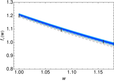
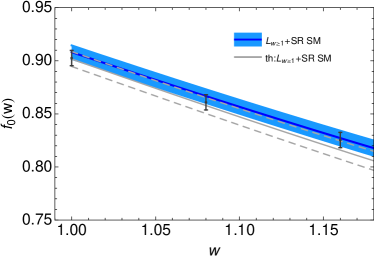
In the “th:Lw1+SRsubscriptth:L𝑤1SR\text{th:}\text{L}_{w\geq 1}{+\text{SR}}” scenario, which uses no experimental data, fitting the parametrized ξ(w)𝜉𝑤\xi(w) to the six lattice points for f+,0(w)subscript𝑓0𝑤f_{+,0}(w) in Table 3 and (1)1\mathcal{F}(1) in Eq. (35), results in a slope parameter

ρ¯2=1.24±0.08.superscriptsubscript¯𝜌2plus-or-minus1.240.08\bar{\rho}_{*}^{2}=1.24\pm 0.08\,. (38)

The fitted w𝑤w spectra are shown in Fig. 1 (gray curves), together with the lattice data points. The χ2superscript𝜒2\chi^{2} of the fit is 7.4, corresponding to a fit probability of 11% with 73=47347-3=4 degrees of freedom. The value for the slope is in good agreement with the slope obtained from the QCDSR constrained and unconstrained “Lw=1subscriptL𝑤1\text{L}_{w=1}” and “NoL” fits.

Form factor w=1.0𝑤1.0w=1.0 w=1.08𝑤1.08w=1.08 w=1.16𝑤1.16w=1.16
f+subscript𝑓f_{+} 1.1994±0.0095plus-or-minus1.19940.00951.1994\pm 0.0095 1.0941±0.0104plus-or-minus1.09410.01041.0941\pm 0.0104 1.0047±0.0123plus-or-minus1.00470.01231.0047\pm 0.0123
f0subscript𝑓0f_{0} 0.9026±0.0072plus-or-minus0.90260.00720.9026\pm 0.0072 0.8609±0.0077plus-or-minus0.86090.00770.8609\pm 0.0077 0.8254±0.0094plus-or-minus0.82540.00940.8254\pm 0.0094
Table 3: The predictions for the form factors f+,0subscript𝑓0f_{+,0} at w=1.0, 1.08, 1.16𝑤1.01.081.16w=1.0,\,1.08,\,1.16 using the synthetic data results of Ref. Bailey et al. (2015). The correlations can be found in Table VII in Ref. Bailey et al. (2015).
Refer to caption
Refer to caption
Figure 1: The “th:Lw1+SRsubscriptth:L𝑤1SR\text{th:}\text{L}_{w\geq 1}{+\text{SR}}” fit of the form factors f+,0subscript𝑓0f_{+,0} to the lattice points listed in Table 3 is shown (gray solid line). The dashed gray lines correspond to the 68% errors. The dark blue line shows the f+,0subscript𝑓0f_{+,0} best fit for “Lw1+SRsubscriptL𝑤1SR\text{L}_{w\geq 1}{+\text{SR}}”, using lattice points, experimental information, and QCDSR constraints. The blue band displays the corresponding 68% CL of this fit.
[Uncaptioned image]
[Uncaptioned image]
[Uncaptioned image]
[Uncaptioned image]
Figure 2: The measured B¯D()lν¯¯𝐵superscript𝐷𝑙¯𝜈{\,\overline{\!B}{}\to D^{(*)}l\bar{\nu}} decay distributions Glattauer et al. (2016); Abdesselam et al. (2017) compared to the best fit contours (dark blue curves) for the “Lw1+SRsubscriptL𝑤1SR\text{L}_{w\geq 1}{+\text{SR}}” fit, using LQCD at all w𝑤w and QCDSR constraints. The blue bands show the 68% CL regions. The orange curves and bands show the central values and the 68% CL regions of the fit predictions for dΓ(B¯D()τν¯)/dwdΓ¯𝐵superscript𝐷𝜏¯𝜈d𝑤{\rm d}\Gamma({\,\overline{\!B}{}\to D^{(*)}\tau\bar{\nu}})/{\rm d}w.

In the “Lw1subscriptL𝑤1\text{L}_{w\geq 1}” fit, all six lattice points for f+,0(w)subscript𝑓0𝑤f_{+,0}(w) in Table 3 and (1)1\mathcal{F}(1) in Eq. (35) are fitted together with the available experimental information. Once again, η(1)superscript𝜂1\eta^{\prime}(1) is fixed to zero, as it is strongly correlated with ρ¯2superscriptsubscript¯𝜌2\bar{\rho}_{*}^{2}. The fit has χ2=49superscript𝜒249\chi^{2}=49, corresponding to a fit probability of 43%. For |Vcb|subscript𝑉𝑐𝑏|V_{cb}|, this fit yields

|Vcb|=(39.1±1.1)×103,subscript𝑉𝑐𝑏plus-or-minus39.11.1superscript103|V_{cb}|=(39.1\pm 1.1)\times 10^{-3}\,, (39)

which is slightly higher than the “Lw=1subscriptL𝑤1\text{L}_{w=1}” result. The value of ρ¯2superscriptsubscript¯𝜌2\bar{\rho}_{*}^{2} is also higher.

In the “Lw1+SRsubscriptL𝑤1SR\text{L}_{w\geq 1}{+\text{SR}}” fit, the QCDSR constraints are included, so that all theory and experimental information is incorporated. The resulting differential B¯D()lν¯¯𝐵superscript𝐷𝑙¯𝜈{\,\overline{\!B}{}\to D^{(*)}l\bar{\nu}} distributions are shown in Fig. III.4, overlaid with the experimental data, as well as the predictions for the B¯D()τν¯¯𝐵superscript𝐷𝜏¯𝜈{\,\overline{\!B}{}\to D^{(*)}\tau\bar{\nu}} differential rates. The fit has χ2=53.8superscript𝜒253.8\chi^{2}=53.8, corresponding to a fit probability of 44%. For |Vcb|subscript𝑉𝑐𝑏|V_{cb}| the fit gives

|Vcb|=(39.3±1.0)×103.subscript𝑉𝑐𝑏plus-or-minus39.31.0superscript103|V_{cb}|=(39.3\pm 1.0)\times 10^{-3}\,. (40)

This is higher than the “Lw=1+SRsubscriptL𝑤1SR\text{L}_{w=1}{+\text{SR}}” result, because the value of ρ¯2superscriptsubscript¯𝜌2\bar{\rho}_{*}^{2} is also higher.

The correlation matrices for all fits are shown in Appendix B. In the “Lw=1subscriptL𝑤1\text{L}_{w=1}” and “Lw1subscriptL𝑤1\text{L}_{w\geq 1}” type fits, moderate correlations are seen between |Vcb|subscript𝑉𝑐𝑏|V_{cb}|, 𝒢(1)𝒢1\mathcal{G}(1), and (1)1\mathcal{F}(1), as expected. The correlations are sizable in these fits between ρ¯2superscriptsubscript¯𝜌2\bar{\rho}_{*}^{2} and the subleading Isgur-Wise functions.

A more detailed study of these effects, in particular the extraction of |Vcb|subscript𝑉𝑐𝑏|V_{cb}|, will be presented elsewhere Bernlochner et al. (2017a). A first comparison with the CLN parametrization Caprini et al. (1998), as implemented by previous experimental studies, can be done by considering the results for the form factor ratios R1subscript𝑅1R_{1} and R2subscript𝑅2R_{2}, defined in Eq. (20). Figure 4 shows the extracted values of R1,2(1)subscript𝑅121R_{1,2}(1) for all fit scenarios. The results agree with each other and with the world average of R1(1)subscript𝑅11R_{1}(1) and R2(1)subscript𝑅21R_{2}(1) Amhis et al. (2016) shown by black ellipses, up to a mild 1σ1𝜎1\sigma tension. Firm conclusions are difficult to reach, as it is impossible to assess how the experimental results would change, had the uncertainties in the quadratic polynomials used to fit R1,2(w)subscript𝑅12𝑤R_{1,2}(w) been properly included. When the QCDSR constraints are used, the central values satisfy R1(1)<1.34subscript𝑅111.34R_{1}(1)<1.34, as required by the HQET prediction in Eq. (II.4) and the constraint η(1)>0𝜂10\eta(1)>0.

Refer to caption
Refer to caption
Figure 3: The SM predictions for R1(1)subscript𝑅11R_{1}(1) and R2(1)subscript𝑅21R_{2}(1) for the fits imposing (left) or not imposing (right) the QCDSR constraints in Eq. (34). The black ellipse shows the world average of the data Amhis et al. (2016). The fit scenarios are described in the text and in Table 1, and the fit results are shown in Table III.4. All contours correspond to 68% CL in two dimensions (Δχ2=χscan2χmin2=2.3Δsuperscript𝜒2subscriptsuperscript𝜒2scansubscriptsuperscript𝜒2min2.3\Delta\chi^{2}=\chi^{2}_{\rm scan}-\chi^{2}_{\rm min}=2.3).
Refer to caption
Refer to caption
Figure 4: The SM predictions for R(D)𝑅𝐷R(D) and R(D)𝑅superscript𝐷R(D^{*}), imposing (left) or not imposing (right) the QCDSR constraints (see Table 4). Gray ellipses show other SM predictions (last three rows of Table 4). The black ellipse shows the world average of the data Amhis et al. (2016). The contours are 68% CL (Δχ2=2.3Δsuperscript𝜒22.3\Delta\chi^{2}=2.3), hence the nearly 4σ4𝜎4\sigma tension.

III.5 R(D())𝑅superscript𝐷R(D^{(*)}) and new physics

Using the fitted values for ρ¯2superscriptsubscript¯𝜌2\bar{\rho}_{*}^{2}, χ^2(1)subscript^𝜒21\hat{\chi}_{2}(1), χ^2(1)subscriptsuperscript^𝜒21\hat{\chi}^{\prime}_{2}(1), χ^3(1)subscriptsuperscript^𝜒31\hat{\chi}^{\prime}_{3}(1), η(1)𝜂1\eta(1), and η(1)superscript𝜂1\eta^{\prime}(1), one can predict R(D())𝑅superscript𝐷R(D^{(*)}) in the SM and for any new physics four-fermion interaction. Figure 4 and Table 4 summarize the predicted values of R(D())𝑅superscript𝐷R(D^{(*)}) in the SM for the seven fit scenarios considered. Our fit results for R(D)𝑅𝐷R(D) are in good agreement with other predictions in the literature Aoki et al. (2016); Bigi and Gambino (2016). All our fits using lattice QCD inputs yield R(D)𝑅superscript𝐷R(D^{*}) above those in Ref. Fajfer et al. (2012). This slightly eases the disagreement with the world average measurement Amhis et al. (2016). The significance is calculated from χ2superscript𝜒2\chi^{2} statistics, taking into account the full covariance of the theory prediction and the world average measurement. The tension between our most precise “Lw1+SRsubscriptL𝑤1SR\text{L}_{w\geq 1}{+\text{SR}}” fit and the data is 3.9σ3.9𝜎3.9\sigma, with a p𝑝p-value of 11.5×10511.5superscript10511.5\times 10^{-5}, to be compared with 8.3×1058.3superscript1058.3\times 10^{-5} quoted by HFAG Amhis et al. (2016). The precision of this prediction is limited by that of the input measurements and LQCD inputs, and can be systematically improved with new data from Belle II or LHCb.

Scenario R(D)𝑅𝐷R(D) R(D)𝑅superscript𝐷R(D^{*}) Correlation
Lw=1subscriptL𝑤1\text{L}_{w=1} 0.292±0.005plus-or-minus0.2920.0050.292\pm 0.005 0.255±0.005plus-or-minus0.2550.0050.255\pm 0.005 41%
Lw=1+SRsubscriptL𝑤1SR\text{L}_{w=1}{+\text{SR}} 0.291±0.005plus-or-minus0.2910.0050.291\pm 0.005 0.255±0.003plus-or-minus0.2550.0030.255\pm 0.003 57%
NoL 0.273±0.016plus-or-minus0.2730.0160.273\pm 0.016 0.250±0.006plus-or-minus0.2500.0060.250\pm 0.006 49%
NoL+SRNoLSR\text{NoL}{+\text{SR}} 0.295±0.007plus-or-minus0.2950.0070.295\pm 0.007 0.255±0.004plus-or-minus0.2550.0040.255\pm 0.004 43%
Lw1subscriptL𝑤1\text{L}_{w\geq 1} 0.298±0.003plus-or-minus0.2980.0030.298\pm 0.003 0.261±0.004plus-or-minus0.2610.0040.261\pm 0.004 19%
Lw1+SRsubscriptL𝑤1SR\text{L}_{w\geq 1}{+\text{SR}} 0.299±0.003plus-or-minus0.2990.003\bm{0.299\pm 0.003} 0.257±0.003plus-or-minus0.2570.003\bm{0.257\pm 0.003} 𝟒𝟒44\bm{44}%
th:Lw1+SRsubscriptth:L𝑤1SR\text{th:}\text{L}_{w\geq 1}{+\text{SR}} 0.306±0.005plus-or-minus0.3060.0050.306\pm 0.005 0.256±0.004plus-or-minus0.2560.0040.256\pm 0.004 33%
Data Amhis et al. (2016) 0.403±0.047plus-or-minus0.4030.0470.403\pm 0.047 0.310±0.017plus-or-minus0.3100.0170.310\pm 0.017 23%percent23-23\%
Refs. Aoki et al. (2016); Bailey et al. (2015); Na et al. (2015) 0.300±0.008plus-or-minus0.3000.0080.300\pm 0.008
Ref. Bigi and Gambino (2016) 0.299±0.003plus-or-minus0.2990.0030.299\pm 0.003
Ref. Fajfer et al. (2012) 0.252±0.003plus-or-minus0.2520.0030.252\pm 0.003
Table 4: The R(D)𝑅𝐷R(D) and R(D)𝑅superscript𝐷R(D^{*}) predictions for our fit scenarios, the world average of the data, and other theory predictions. The fit scenarios are described in the text and in Table 1. The bold numbers are our most precise predictions.

To derive a SM prediction for R(D)𝑅superscript𝐷R(D^{*}), Ref. Fajfer et al. (2012) used the measured R2(1)subscript𝑅21R_{2}(1) form factor ratio Amhis et al. (2016) and the QCDSR predictions to obtain R0(1)=1.14±0.11subscript𝑅01plus-or-minus1.140.11R_{0}(1)=1.14\pm 0.11. In comparison, our “Lw1+SRsubscriptL𝑤1SR\text{L}_{w\geq 1}{+\text{SR}}” fit results yield

R0(1)=1.17±0.02,R3(1)=1.19±0.03.formulae-sequencesubscript𝑅01plus-or-minus1.170.02subscript𝑅31plus-or-minus1.190.03R_{0}(1)=1.17\pm 0.02\,,\qquad R_{3}(1)=1.19\pm 0.03\,. (41)

The precision on R0(1)subscript𝑅01R_{0}(1) improves five-fold compared to Ref. Fajfer et al. (2012) and is in good agreement.
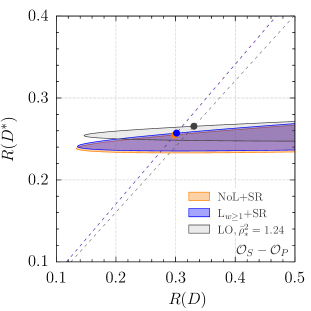
Refer to caption Refer to caption

Refer to caption Refer to caption

Figure 5: The allowed ranges of R(D)R(D)𝑅𝐷𝑅superscript𝐷R(D)-R(D^{*}), due to one of the new physics operators in addition to the SM: OSOPsubscript𝑂𝑆subscript𝑂𝑃O_{S}-O_{P} (top left), OS+OPsubscript𝑂𝑆subscript𝑂𝑃O_{S}+O_{P} (top right), OV+OAsubscript𝑂𝑉subscript𝑂𝐴O_{V}+O_{A} (bottom left), OTsubscript𝑂𝑇O_{T} (bottom right).

In Fig. 5 we illustrate the impacts NP might have on the allowed R(D)R(D)𝑅𝐷𝑅superscript𝐷R(D)-R(D^{*}) regions, assuming the dominance of one new physics operator in a standard four-Fermi basis. NP couplings are permitted to have an arbitrary phase, generating allowed regions rather than single contours. We display the allowed regions generated for the “NoL+SRNoLSR\text{NoL}{+\text{SR}}” best fit values; the “Lw1+SRsubscriptL𝑤1SR\text{L}_{w\geq 1}{+\text{SR}}” best fit values; and for leading order contributions only, i.e., αssubscript𝛼𝑠\alpha_{s}, εc,b0subscript𝜀𝑐𝑏0\varepsilon_{c,b}\to 0, with ρ¯2=1.24superscriptsubscript¯𝜌21.24\bar{\rho}_{*}^{2}=1.24. The small variation between the “NoL+SRNoLSR\text{NoL}{+\text{SR}}” and “Lw1+SRsubscriptL𝑤1SR\text{L}_{w\geq 1}{+\text{SR}}” regions illustrates the good consistency of the predictions obtained with and without LQCD. On each plot, we also include for comparison the corresponding contours (dashed lines) produced by a NP OVOAsubscript𝑂𝑉subscript𝑂𝐴O_{V}-O_{A} coupling. The latter rescales R(D)𝑅𝐷R(D) and R(D)𝑅superscript𝐷R(D^{*}) keeping their ratio fixed. Solid dots indicate the SM point for each case. For scalar currents, if NP only contributes to OSsubscript𝑂𝑆O_{S} (OPsubscript𝑂𝑃O_{P}) then only R(D)𝑅𝐷R(D) (R(D)𝑅superscript𝐷R(D^{*})) is affected in accordance with Eq. (10b) (Eq. (11a)), respectively. We plot the allowed regions for the OS±OPplus-or-minussubscript𝑂𝑆subscript𝑂𝑃O_{S}\pm O_{P} linear combinations, which are also motivated by specific NP models.

IV Summary and Outlook

We performed a novel combined fit of the B¯Dlν¯¯𝐵𝐷𝑙¯𝜈{\,\overline{\!B}{}\to Dl\bar{\nu}} and B¯Dlν¯¯𝐵superscript𝐷𝑙¯𝜈{\,\overline{\!B}{}\to D^{*}l\bar{\nu}} differential rates and angular distributions, consistently including the HQET relations to 𝒪(ΛQCD/mc,b,αs)𝒪subscriptΛQCDsubscript𝑚𝑐𝑏subscript𝛼𝑠\mathcal{O}(\Lambda_{\rm QCD}/{m_{c,b}},\,\alpha_{s}). Under various fit scenarios, that use or omit lattice QCD and QCD sum rule predictions, we constrain the leading and subleading Isgur-Wise functions. We thus obtain strong constraints on all form factors, and predictions for the form factor ratios R1,2subscript𝑅12R_{1,2} as well as R(D())𝑅superscript𝐷R(D^{(*)}), both in the SM and in arbitrary NP scenarios, valid at 𝒪(αs)𝒪subscript𝛼𝑠\mathcal{O}(\alpha_{s}) and 𝒪(ΛQCD/mc,b)𝒪subscriptΛQCDsubscript𝑚𝑐𝑏\mathcal{O}(\Lambda_{\rm QCD}/m_{c,b}). Our most precise prediction for R(D())𝑅superscript𝐷R(D^{(*)}), in the “Lw1+SRsubscriptL𝑤1SR\text{L}_{w\geq 1}{+\text{SR}}” fit, using the experimental data and all lattice QCD and QCDSR inputs is

R(D)=0.299±0.003,R(D)=0.257±0.003,formulae-sequence𝑅𝐷plus-or-minus0.2990.003𝑅superscript𝐷plus-or-minus0.2570.003R(D)=0.299\pm 0.003\,,\qquad R(D^{*})=0.257\pm 0.003\,, (42)

with a correlation of 44%. The same fit also yields |Vcb|=(39.3±1.0)×103subscript𝑉𝑐𝑏plus-or-minus39.31.0superscript103|V_{cb}|=(39.3\pm 1.0)\times 10^{-3}, which is in good agreement with existing exclusive determinations. All possible bc𝑏𝑐b\to c current form factors are derived at 𝒪(ΛQCD/mc,b)𝒪subscriptΛQCDsubscript𝑚𝑐𝑏\mathcal{O}(\Lambda_{\rm QCD}/m_{c,b}) and 𝒪(αs)𝒪subscript𝛼𝑠\mathcal{O}(\alpha_{s}), including those for a tensor current, previously unavailable in the literature at this order. A lattice QCD calculation of the subleading Isgur-Wise functions, or even just those which arise from the chromomagnetic term in the subleading HQET Lagrangian (χ2,3subscript𝜒23\chi_{2,3}), would be important to reduce hadronic uncertainties in both SM and NP predictions, complementary to a long-awaited lattice calculation of R(D)𝑅superscript𝐷R(D^{*}).

At the current level of experimental precision, our predictions agree up to mild tensions with previous results, which neglected the HQET relations for the uncertainties of the 𝒪(ΛQCD/mc,b)𝒪subscriptΛQCDsubscript𝑚𝑐𝑏\mathcal{O}(\Lambda_{\rm QCD}/m_{c,b}) terms. Our fit results are consistent with one another, and at the current level of precision we find no inconsistencies between the data, lattice QCD results, and QCD sum rule predictions. Our fit using all available lattice QCD and QCD sum rule inputs and HQET to order 𝒪(αs,ΛQCD/mc,b)𝒪subscript𝛼𝑠subscriptΛQCDsubscript𝑚𝑐𝑏\mathcal{O}(\alpha_{s},\Lambda_{\rm QCD}/m_{c,b}) yields the most precise combined prediction for R(D)𝑅𝐷R(D) and R(D)𝑅superscript𝐷R(D^{*}) to date. However, in principle, our fit need not require either lattice or sum rule input, and its precision can be improved simply as the statistics of future data increases.

The (moderate) tension between the measurements of |Vcb|subscript𝑉𝑐𝑏|V_{cb}| from inclusive and exclusive semileptonic decays probably cannot be resolved with current data. Understanding how the inclusive rate is made up from a sum of exclusive channels has been unclear from the data for a long time Richman and Burchat (1995), and puzzles remain even in light of BaBar and Belle measurements Bernlochner et al. (2012, 2014). A more detailed examination of the effects of the unitarity constraints and the precision extraction of |Vcb|subscript𝑉𝑐𝑏|V_{cb}| is the subject of ongoing work Bernlochner et al. (2017a). We are also implementing the full angular distributions of the measurable particles Ligeti et al. (2017); Alonso et al. (2016) into a software package, hammer Duell et al. (2017); Bernlochner et al. (2017b), based on the state-of-the-art HQET predictions for all six BD,D,D𝐵𝐷superscript𝐷superscript𝐷absentB\to D,D^{*},D^{**} decay modes.

Acknowledgements.
We thank Marat Freytsis, Ben Grinstein and Aneesh Manohar for helpful conversations. We thank Martin Jung for pointing out typos in Eqs. (43a) and (43b) in an earlier version. FB was supported by the DFG Emmy-Noether Grant No. BE 6075/1-1. FB thanks Kim Scott and Robert Michaud for the kind hospitality in Houston where part of this work was carried out and inspiring conversations over good wine and food. ZL and MP were supported in part by the U.S. Department of Energy under contract DE-AC02-05CH11231. DR acknowledges support from the University of Cincinnati.

Appendix A The 𝒪(αs)𝒪subscript𝛼𝑠\mathcal{O}(\alpha_{s}) corrections

In this appendix we summarize the explicit expressions for the CΓ(w)subscript𝐶Γ𝑤C_{\Gamma}(w) functions defined in Eq. (II.1), calculated in Ref. Neubert (1992). The following results use the MS¯¯MS\overline{\rm MS} scheme and correspond to matching from QCD onto HQET at μ=mcmb𝜇subscript𝑚𝑐subscript𝑚𝑏\mu=\sqrt{m_{c}m_{b}},

CSsubscript𝐶𝑆\displaystyle C_{S} =13z(wwz)[2z(wwz)Ω(w)(w1)(z+1)2r(w)+(z21)lnz],absent13𝑧𝑤subscript𝑤𝑧delimited-[]2𝑧𝑤subscript𝑤𝑧Ω𝑤𝑤1superscript𝑧12𝑟𝑤superscript𝑧21𝑧\displaystyle=\frac{1}{3z(w-w_{z})}\Big{[}2z(w-w_{z})\Omega(w)-(w-1)(z+1)^{2}r(w)+(z^{2}-1)\ln z\Big{]}, (43a)
CPsubscript𝐶𝑃\displaystyle C_{P} =13z(wwz)[2z(wwz)Ω(w)(w+1)(z1)2r(w)+(z21)lnz],absent13𝑧𝑤subscript𝑤𝑧delimited-[]2𝑧𝑤subscript𝑤𝑧Ω𝑤𝑤1superscript𝑧12𝑟𝑤superscript𝑧21𝑧\displaystyle=\frac{1}{3z(w-w_{z})}\Big{[}2z(w-w_{z})\Omega(w)-(w+1)(z-1)^{2}r(w)+(z^{2}-1)\ln z\Big{]}, (43b)
CV1subscript𝐶subscript𝑉1\displaystyle C_{V_{1}} =16z(wwz)[2(w+1)((3w1)zz21)r(w)\displaystyle=\frac{1}{6z(w-w_{z})}\Big{[}2(w+1)\big{(}(3w-1)z-z^{2}-1\big{)}r(w)
+(12z(wzw)(z21)lnz)+4z(wwz)Ω(w)],\displaystyle\qquad\qquad\qquad\qquad+\big{(}12z(w_{z}-w)-(z^{2}-1)\ln z\big{)}+4z(w-w_{z})\Omega(w)\Big{]}, (43c)
CV2subscript𝐶subscript𝑉2\displaystyle C_{V_{2}} =16z2(wwz)2[((4w2+2w)z2(2w2+5w1)z(w+1)z3+2)r(w)\displaystyle=\frac{-1}{6z^{2}(w-w_{z})^{2}}\Big{[}\big{(}(4w^{2}+2w)z^{2}-(2w^{2}+5w-1)z-(w+1)z^{3}+2\big{)}r(w)
+z(2(z1)(wzw)+(z2(4w2)z+(32w))lnz)],\displaystyle\qquad\qquad\qquad\qquad+z\big{(}2(z-1)(w_{z}-w)+\big{(}z^{2}-(4w-2)z+(3-2w)\big{)}\ln z\big{)}\Big{]}, (43d)
CV3subscript𝐶subscript𝑉3\displaystyle C_{V_{3}} =16z(wwz)2[((2w2+5w1)z2(4w2+2w)z2z3+w+1)r(w)\displaystyle=\frac{1}{6z(w-w_{z})^{2}}\Big{[}\big{(}(2w^{2}+5w-1)z^{2}-(4w^{2}+2w)z-2z^{3}+w+1\big{)}r(w)
+(2z(z1)(wzw)+((32w)z2+(24w)z+1)lnz)],\displaystyle\qquad\qquad\qquad\qquad+\big{(}2z(z-1)(w_{z}-w)+((3-2w)z^{2}+(2-4w)z+1)\ln z\big{)}\Big{]}, (43e)
CA1subscript𝐶subscript𝐴1\displaystyle C_{A_{1}} =16z(wwz)[2(w1)((3w+1)zz21)r(w)\displaystyle=\frac{1}{6z(w-w_{z})}\Big{[}2(w-1)\big{(}(3w+1)z-z^{2}-1\big{)}r(w)
+(12z(wzw)(z21)lnz)+4z(wwz)Ω(w)],\displaystyle\qquad\qquad\qquad\qquad+\big{(}12z(w_{z}-w)-(z^{2}-1)\ln z\big{)}+4z(w-w_{z})\Omega(w)\Big{]}, (43f)
CA2subscript𝐶subscript𝐴2\displaystyle C_{A_{2}} =16z2(wwz)2[((4w22w)z2+(2w25w1)z+(1w)z3+2)r(w)\displaystyle=\frac{-1}{6z^{2}(w-w_{z})^{2}}\Big{[}\big{(}(4w^{2}-2w)z^{2}+(2w^{2}-5w-1)z+(1-w)z^{3}+2\big{)}r(w)
+z(2(z+1)(wzw)+(z2(4w+2)z+(2w+3))lnz)],\displaystyle\qquad\qquad\qquad\qquad+z\big{(}2(z+1)(w_{z}-w)+\big{(}z^{2}-(4w+2)z+(2w+3)\big{)}\ln z\big{)}\Big{]}, (43g)
CA3subscript𝐶subscript𝐴3\displaystyle C_{A_{3}} =16z(wwz)2[(2z3+(2w25w1)z2+(4w22w)zw+1)r(w)\displaystyle=\frac{1}{6z(w-w_{z})^{2}}\Big{[}\big{(}2z^{3}+(2w^{2}-5w-1)z^{2}+(4w^{2}-2w)z-w+1\big{)}r(w)
+(2z(z+1)(wzw)((2w+3)z2(4w+2)z+1)lnz)],\displaystyle\qquad\qquad\qquad\qquad+\!\big{(}2z(z+1)(w_{z}-w)-\big{(}(2w+3)z^{2}-(4w+2)z+1\big{)}\ln z\big{)}\Big{]}, (43h)
CT1subscript𝐶subscript𝑇1\displaystyle C_{T_{1}} =13z(wwz)[(w1)((4w+2)zz21)r(w)\displaystyle=\frac{1}{3z(w-w_{z})}\Big{[}(w-1)\big{(}(4w+2)z-z^{2}-1\big{)}r(w)
+(6z(wzw)(z21)lnz)+2z(wwz)Ω(w)],\displaystyle\qquad\qquad\qquad\qquad+\big{(}6z(w_{z}-w)-(z^{2}-1)\ln z\big{)}+2z(w-w_{z})\Omega(w)\Big{]}, (43i)
CT2subscript𝐶subscript𝑇2\displaystyle C_{T_{2}} =23z(wwz)[(1wz)r(w)+zlnz],absent23𝑧𝑤subscript𝑤𝑧delimited-[]1𝑤𝑧𝑟𝑤𝑧𝑧\displaystyle=\frac{2}{3z(w-w_{z})}\Big{[}(1-wz)r(w)+z\ln z\Big{]}, (43j)
CT3subscript𝐶subscript𝑇3\displaystyle C_{T_{3}} =23(wwz)[(wz)r(w)+lnz],absent23𝑤subscript𝑤𝑧delimited-[]𝑤𝑧𝑟𝑤𝑧\displaystyle=\frac{2}{3(w-w_{z})}\Big{[}(w-z)r(w)+\ln z\Big{]}, (43k)

and CT4=0subscript𝐶subscript𝑇40C_{T_{4}}=0. Here z=mc/mb𝑧subscript𝑚𝑐subscript𝑚𝑏z=m_{c}/m_{b}, and the functions

Ω(w)w2w21[2Li2(1wz)2Li2(1w+z)+Li2(1w+2)Li2(1w2)]wr(w)lnz+1,Ω𝑤𝑤2superscript𝑤21delimited-[]2subscriptLi21subscript𝑤𝑧2subscriptLi21subscript𝑤𝑧subscriptLi21superscriptsubscript𝑤2subscriptLi21superscriptsubscript𝑤2𝑤𝑟𝑤𝑧1\Omega(w)\equiv\frac{w}{2\sqrt{w^{2}-1}}\big{[}2\text{Li}_{2}(1-w_{-}z)-2\text{Li}_{2}(1-w_{+}z)+\text{Li}_{2}(1-w_{+}^{2})-\text{Li}_{2}(1-w_{-}^{2})\big{]}\\ -w\,r(w)\ln z+1\,, (44)

where Li2(x)=x0ln(1t)/tdtsubscriptLi2𝑥superscriptsubscript𝑥01𝑡𝑡differential-d𝑡\text{Li}_{2}(x)=\int_{x}^{0}\ln(1-t)/t\,{\rm d}t is the dilogarithm, and

r(w)lnw+w21,w±w±w21,wz12(z+1/z).formulae-sequence𝑟𝑤subscript𝑤superscript𝑤21formulae-sequencesubscript𝑤plus-or-minusplus-or-minus𝑤superscript𝑤21subscript𝑤𝑧12𝑧1𝑧r(w)\equiv\frac{\ln w_{+}}{\sqrt{w^{2}-1}}\,,\qquad w_{\pm}\equiv w\pm\sqrt{w^{2}-1}\,,\qquad w_{z}\equiv\frac{1}{2}\,\big{(}z+1/z\big{)}\,. (45)

At the zero recoil point, w=1𝑤1w=1,

CS(1)subscript𝐶𝑆1\displaystyle C_{S}(1) =23,CP(1)=23,formulae-sequenceabsent23subscript𝐶𝑃123\displaystyle=-\frac{2}{3}\,,\qquad C_{P}(1)=\frac{2}{3}\,,
CV1(1)subscript𝐶subscript𝑉11\displaystyle C_{V_{1}}(1) =431+z1zlnz,CV2(1)=2(1z+zlnz)3(1z)2,CV3(1)=2z(1z+lnz)3(1z)2,formulae-sequenceabsent431𝑧1𝑧𝑧formulae-sequencesubscript𝐶subscript𝑉2121𝑧𝑧𝑧3superscript1𝑧2subscript𝐶subscript𝑉312𝑧1𝑧𝑧3superscript1𝑧2\displaystyle=-\frac{4}{3}-\frac{1+z}{1-z}\ln z,\quad C_{V_{2}}(1)=-\frac{2\,(1-z+z\ln z)}{3(1-z)^{2}}\,,\quad C_{V_{3}}(1)=\frac{2z(1-z+\ln z)}{3(1-z)^{2}}\,,
CA1(1)subscript𝐶subscript𝐴11\displaystyle C_{A_{1}}(1) =831+z1zlnz,absent831𝑧1𝑧𝑧\displaystyle=-\frac{8}{3}-\frac{1+z}{1-z}\,\ln z\,,
CA2(1)subscript𝐶subscript𝐴21\displaystyle C_{A_{2}}(1) =2[32zz2+(5z)zlnz]3(1z)3,CA3(1)=2z[1+2z3z2+(5z1)lnz]3(1z)3,formulae-sequenceabsent2delimited-[]32𝑧superscript𝑧25𝑧𝑧𝑧3superscript1𝑧3subscript𝐶subscript𝐴312𝑧delimited-[]12𝑧3superscript𝑧25𝑧1𝑧3superscript1𝑧3\displaystyle=-\frac{2\,[3-2z-z^{2}+(5-z)z\ln z]}{3(1-z)^{3}}\,,\qquad C_{A_{3}}(1)=\frac{2z\,[1+2z-3z^{2}+(5z-1)\ln z]}{3(1-z)^{3}}\,,
CT1(1)subscript𝐶subscript𝑇11\displaystyle C_{T_{1}}(1) =834(1+z)3(1z)lnz,CT2(1)=2CV2(1),CT3(1)=2CV3(1).formulae-sequenceabsent8341𝑧31𝑧𝑧formulae-sequencesubscript𝐶subscript𝑇212subscript𝐶subscript𝑉21subscript𝐶subscript𝑇312subscript𝐶subscript𝑉31\displaystyle=-\frac{8}{3}-\frac{4(1+z)}{3(1-z)}\,\ln z\,,\qquad C_{T_{2}}(1)=2\,C_{V_{2}}(1)\,,\qquad C_{T_{3}}(1)=-2\,C_{V_{3}}(1)\,. (46)

Finally, for arbitrary matching scale μ𝜇\mu, one should add to Eqs. (43) the terms

CS,P(μ2)superscriptsubscript𝐶𝑆𝑃superscript𝜇2\displaystyle C_{S,P}^{(\mu^{2})} =CS,P(mbmc)13[2wr(w)+1]ln(mcmb/μ2),absentsuperscriptsubscript𝐶𝑆𝑃subscript𝑚𝑏subscript𝑚𝑐13delimited-[]2𝑤𝑟𝑤1subscript𝑚𝑐subscript𝑚𝑏superscript𝜇2\displaystyle=C_{S,P}^{(m_{b}m_{c})}-\frac{1}{3}\,[2w\,r(w)+1]\ln(m_{c}m_{b}/\mu^{2})\,, (47a)
CV1,A1(μ2)superscriptsubscript𝐶subscript𝑉1subscript𝐴1superscript𝜇2\displaystyle C_{V_{1},A_{1}}^{(\mu^{2})} =CV1,A1(mbmc)23[wr(w)1]ln(mcmb/μ2),absentsuperscriptsubscript𝐶subscript𝑉1subscript𝐴1subscript𝑚𝑏subscript𝑚𝑐23delimited-[]𝑤𝑟𝑤1subscript𝑚𝑐subscript𝑚𝑏superscript𝜇2\displaystyle=C_{V_{1},A_{1}}^{(m_{b}m_{c})}-\frac{2}{3}\,[w\,r(w)-1]\ln(m_{c}m_{b}/\mu^{2})\,, (47b)
CT1(μ2)superscriptsubscript𝐶subscript𝑇1superscript𝜇2\displaystyle C_{T_{1}}^{(\mu^{2})} =CT1(mbmc)13[2wr(w)3]ln(mcmb/μ2),absentsuperscriptsubscript𝐶subscript𝑇1subscript𝑚𝑏subscript𝑚𝑐13delimited-[]2𝑤𝑟𝑤3subscript𝑚𝑐subscript𝑚𝑏superscript𝜇2\displaystyle=C_{T_{1}}^{(m_{b}m_{c})}-\frac{1}{3}\,[2w\,r(w)-3]\ln(m_{c}m_{b}/\mu^{2})\,, (47c)

and all other CΓj(μ2)=CΓj(mbmc)superscriptsubscript𝐶subscriptΓ𝑗superscript𝜇2superscriptsubscript𝐶subscriptΓ𝑗subscript𝑚𝑏subscript𝑚𝑐C_{\Gamma_{j}}^{(\mu^{2})}=C_{\Gamma_{j}}^{(m_{b}m_{c})}, for j2𝑗2j\geq 2.

Appendix B Dull Correlations

The correlation matrices for the fit scenarios are given in Tables 5-11.

|Vcb|subscript𝑉𝑐𝑏|V_{cb}| 𝒢(1)𝒢1\mathcal{G}(1) (1)1\mathcal{F}(1) ρ¯2superscriptsubscript¯𝜌2\bar{\rho}_{*}^{2} χ^2(1)subscript^𝜒21\hat{\chi}_{2}(1) χ^2(1)superscriptsubscript^𝜒21\hat{\chi}_{2}^{\prime}(1) χ^3(1)superscriptsubscript^𝜒31\hat{\chi}_{3}^{\prime}(1) η(1)𝜂1\eta(1) mb1Ssuperscriptsubscript𝑚𝑏1𝑆m_{b}^{1S} δmbc𝛿subscript𝑚𝑏𝑐\delta m_{bc}
|Vcb|subscript𝑉𝑐𝑏|V_{cb}| 1.001.001.00 0.160.16-0.16 0.180.18-0.18 0.300.300.30 0.130.13-0.13 0.280.280.28 0.110.110.11 0.040.040.04 0.010.01-0.01 0.000.000.00
𝒢(1)𝒢1\mathcal{G}(1) 0.160.16-0.16 1.001.001.00 0.060.060.06 0.110.11-0.11 0.030.030.03 0.040.04-0.04 0.090.09-0.09 0.230.23-0.23 0.000.000.00 0.000.00-0.00
(1)1\mathcal{F}(1) 0.180.18-0.18 0.060.060.06 1.001.001.00 0.180.180.18 0.000.00-0.00 0.080.080.08 0.210.210.21 0.020.02-0.02 0.010.010.01 0.000.00-0.00
ρ¯2superscriptsubscript¯𝜌2\bar{\rho}_{*}^{2} 0.300.300.30 0.110.11-0.11 0.180.180.18 1.001.001.00 0.670.670.67 0.470.47-0.47 0.820.820.82 0.130.130.13 0.160.16-0.16 0.010.010.01
χ^2(1)subscript^𝜒21\hat{\chi}_{2}(1) 0.130.13-0.13 0.030.030.03 0.000.00-0.00 0.670.670.67 1.001.001.00 0.870.87-0.87 0.820.820.82 0.110.11-0.11 0.070.070.07 0.010.01-0.01
χ^2(1)superscriptsubscript^𝜒21\hat{\chi}_{2}^{\prime}(1) 0.280.280.28 0.040.04-0.04 0.080.080.08 0.470.47-0.47 0.870.87-0.87 1.001.001.00 0.470.47-0.47 0.010.010.01 0.010.010.01 0.000.00-0.00
χ^3(1)superscriptsubscript^𝜒31\hat{\chi}_{3}^{\prime}(1) 0.110.110.11 0.090.09-0.09 0.210.210.21 0.820.820.82 0.820.820.82 0.470.47-0.47 1.001.001.00 0.120.12-0.12 0.120.120.12 0.020.02-0.02
η(1)𝜂1\eta(1) 0.040.040.04 0.230.23-0.23 0.020.02-0.02 0.130.130.13 0.110.11-0.11 0.010.010.01 0.120.12-0.12 1.001.001.00 0.520.52-0.52 0.050.050.05
mb1Ssuperscriptsubscript𝑚𝑏1𝑆m_{b}^{1S} 0.010.01-0.01 0.000.000.00 0.010.010.01 0.160.16-0.16 0.070.070.07 0.010.010.01 0.120.120.12 0.520.52-0.52 1.001.001.00 0.000.000.00
δmbc𝛿subscript𝑚𝑏𝑐\delta m_{bc} 0.000.000.00 0.000.00-0.00 0.000.00-0.00 0.010.010.01 0.010.01-0.01 0.000.00-0.00 0.020.02-0.02 0.050.050.05 0.000.000.00 1.001.001.00
Table 5: The correlations of the “Lw=1subscriptL𝑤1\text{L}_{w=1}” fit scenario.
|Vcb|subscript𝑉𝑐𝑏|V_{cb}| 𝒢(1)𝒢1\mathcal{G}(1) (1)1\mathcal{F}(1) ρ¯2superscriptsubscript¯𝜌2\bar{\rho}_{*}^{2} χ^2(1)subscript^𝜒21\hat{\chi}_{2}(1) χ^2(1)superscriptsubscript^𝜒21\hat{\chi}_{2}^{\prime}(1) χ^3(1)superscriptsubscript^𝜒31\hat{\chi}_{3}^{\prime}(1) η(1)𝜂1\eta(1) η(1)superscript𝜂1\eta^{\prime}(1) mb1Ssuperscriptsubscript𝑚𝑏1𝑆m_{b}^{1S} δmbc𝛿subscript𝑚𝑏𝑐\delta m_{bc}
|Vcb|subscript𝑉𝑐𝑏|V_{cb}| 1.001.001.00 0.120.12-0.12 0.320.32-0.32 0.480.480.48 0.020.02-0.02 0.020.020.02 0.140.140.14 0.050.050.05 0.020.020.02 0.020.02-0.02 0.000.000.00
𝒢(1)𝒢1\mathcal{G}(1) 0.120.12-0.12 1.001.001.00 0.140.140.14 0.050.05-0.05 0.040.040.04 0.010.010.01 0.140.14-0.14 0.230.23-0.23 0.090.090.09 0.000.00-0.00 0.000.00-0.00
(1)1\mathcal{F}(1) 0.320.32-0.32 0.140.140.14 1.001.001.00 0.040.040.04 0.070.07-0.07 0.010.01-0.01 0.240.240.24 0.020.02-0.02 0.110.11-0.11 0.030.03-0.03 0.010.010.01
ρ¯2superscriptsubscript¯𝜌2\bar{\rho}_{*}^{2} 0.480.480.48 0.050.05-0.05 0.040.040.04 1.001.001.00 0.090.09-0.09 0.040.04-0.04 0.570.570.57 0.320.320.32 0.080.080.08 0.450.45-0.45 0.040.040.04
χ^2(1)subscript^𝜒21\hat{\chi}_{2}(1) 0.020.02-0.02 0.040.040.04 0.070.07-0.07 0.090.09-0.09 1.001.001.00 0.030.03-0.03 0.170.170.17 0.060.06-0.06 0.200.20-0.20 0.040.040.04 0.000.00-0.00
χ^2(1)superscriptsubscript^𝜒21\hat{\chi}_{2}^{\prime}(1) 0.020.020.02 0.010.010.01 0.010.01-0.01 0.040.04-0.04 0.030.03-0.03 1.001.001.00 0.060.060.06 0.020.02-0.02 0.090.09-0.09 0.010.010.01 0.000.00-0.00
χ^3(1)superscriptsubscript^𝜒31\hat{\chi}_{3}^{\prime}(1) 0.140.140.14 0.140.14-0.14 0.240.240.24 0.570.570.57 0.170.170.17 0.060.060.06 1.001.001.00 0.080.080.08 0.380.380.38 0.030.03-0.03 0.000.000.00
η(1)𝜂1\eta(1) 0.050.050.05 0.230.23-0.23 0.020.02-0.02 0.320.320.32 0.060.06-0.06 0.020.02-0.02 0.080.080.08 1.001.001.00 0.140.14-0.14 0.480.48-0.48 0.050.050.05
η(1)superscript𝜂1\eta^{\prime}(1) 0.020.020.02 0.090.090.09 0.110.11-0.11 0.080.080.08 0.200.20-0.20 0.090.09-0.09 0.380.380.38 0.140.14-0.14 1.001.001.00 0.080.080.08 0.010.01-0.01
mb1Ssuperscriptsubscript𝑚𝑏1𝑆m_{b}^{1S} 0.020.02-0.02 0.000.00-0.00 0.030.03-0.03 0.450.45-0.45 0.040.040.04 0.010.010.01 0.030.03-0.03 0.480.48-0.48 0.080.080.08 1.001.001.00 0.010.010.01
δmbc𝛿subscript𝑚𝑏𝑐\delta m_{bc} 0.000.000.00 0.000.00-0.00 0.010.010.01 0.040.040.04 0.000.00-0.00 0.000.00-0.00 0.000.000.00 0.050.050.05 0.010.01-0.01 0.010.010.01 1.001.001.00
Table 6: The correlations of the “Lw=1+SRsubscriptL𝑤1SR\text{L}_{w=1}{+\text{SR}}” fit scenario.
ρ¯2superscriptsubscript¯𝜌2\bar{\rho}_{*}^{2} χ^2(1)subscript^𝜒21\hat{\chi}_{2}(1) χ^2(1)superscriptsubscript^𝜒21\hat{\chi}_{2}^{\prime}(1) χ^3(1)superscriptsubscript^𝜒31\hat{\chi}_{3}^{\prime}(1) η(1)𝜂1\eta(1) mb1Ssuperscriptsubscript𝑚𝑏1𝑆m_{b}^{1S} δmbc𝛿subscript𝑚𝑏𝑐\delta m_{bc}
ρ¯2superscriptsubscript¯𝜌2\bar{\rho}_{*}^{2} 1.001.001.00 0.220.22-0.22 0.180.18-0.18 0.030.03-0.03 0.460.460.46 0.220.22-0.22 0.010.010.01
χ^2(1)subscript^𝜒21\hat{\chi}_{2}(1) 0.220.22-0.22 1.001.001.00 0.410.41-0.41 0.940.940.94 0.920.92-0.92 0.330.330.33 0.030.03-0.03
χ^2(1)superscriptsubscript^𝜒21\hat{\chi}_{2}^{\prime}(1) 0.180.18-0.18 0.410.41-0.41 1.001.001.00 0.190.19-0.19 0.080.080.08 0.020.02-0.02 0.000.00-0.00
χ^3(1)superscriptsubscript^𝜒31\hat{\chi}_{3}^{\prime}(1) 0.030.03-0.03 0.940.940.94 0.190.19-0.19 1.001.001.00 0.880.88-0.88 0.320.320.32 0.030.03-0.03
η(1)𝜂1\eta(1) 0.460.460.46 0.920.92-0.92 0.080.080.08 0.880.88-0.88 1.001.001.00 0.350.35-0.35 0.020.020.02
mb1Ssuperscriptsubscript𝑚𝑏1𝑆m_{b}^{1S} 0.220.22-0.22 0.330.330.33 0.020.02-0.02 0.320.320.32 0.350.35-0.35 1.001.001.00 0.000.000.00
δmbc𝛿subscript𝑚𝑏𝑐\delta m_{bc} 0.010.010.01 0.030.03-0.03 0.000.00-0.00 0.030.03-0.03 0.020.020.02 0.000.000.00 1.001.001.00
Table 7: The correlations of the “NoL” fit scenario.
ρ¯2superscriptsubscript¯𝜌2\bar{\rho}_{*}^{2} χ^2(1)subscript^𝜒21\hat{\chi}_{2}(1) χ^2(1)superscriptsubscript^𝜒21\hat{\chi}_{2}^{\prime}(1) χ^3(1)superscriptsubscript^𝜒31\hat{\chi}_{3}^{\prime}(1) η(1)𝜂1\eta(1) η(1)superscript𝜂1\eta^{\prime}(1) mb1Ssuperscriptsubscript𝑚𝑏1𝑆m_{b}^{1S} δmbc𝛿subscript𝑚𝑏𝑐\delta m_{bc}
ρ¯2superscriptsubscript¯𝜌2\bar{\rho}_{*}^{2} 1.001.001.00 0.150.15-0.15 0.070.07-0.07 0.570.570.57 0.440.440.44 0.110.11-0.11 0.310.31-0.31 0.030.030.03
χ^2(1)subscript^𝜒21\hat{\chi}_{2}(1) 0.150.15-0.15 1.001.001.00 0.020.02-0.02 0.070.070.07 0.150.15-0.15 0.090.09-0.09 0.020.020.02 0.000.00-0.00
χ^2(1)superscriptsubscript^𝜒21\hat{\chi}_{2}^{\prime}(1) 0.070.07-0.07 0.020.02-0.02 1.001.001.00 0.030.030.03 0.070.07-0.07 0.050.05-0.05 0.000.000.00 0.000.00-0.00
χ^3(1)superscriptsubscript^𝜒31\hat{\chi}_{3}^{\prime}(1) 0.570.570.57 0.070.070.07 0.030.030.03 1.001.001.00 0.170.170.17 0.160.160.16 0.000.000.00 0.000.00-0.00
η(1)𝜂1\eta(1) 0.440.440.44 0.150.15-0.15 0.070.07-0.07 0.170.170.17 1.001.001.00 0.400.40-0.40 0.090.090.09 0.010.01-0.01
η(1)superscript𝜂1\eta^{\prime}(1) 0.110.11-0.11 0.090.09-0.09 0.050.05-0.05 0.160.160.16 0.400.40-0.40 1.001.001.00 0.020.020.02 0.000.00-0.00
mb1Ssuperscriptsubscript𝑚𝑏1𝑆m_{b}^{1S} 0.310.31-0.31 0.020.020.02 0.000.000.00 0.000.000.00 0.090.090.09 0.020.020.02 1.001.001.00 0.010.010.01
δmbc𝛿subscript𝑚𝑏𝑐\delta m_{bc} 0.030.030.03 0.000.00-0.00 0.000.00-0.00 0.000.00-0.00 0.010.01-0.01 0.000.00-0.00 0.010.010.01 1.001.001.00
Table 8: The correlations of the “NoL+SRNoLSR\text{NoL}{+\text{SR}}” fit scenario.
|Vcb|×103subscript𝑉𝑐𝑏superscript103|V_{cb}|\times 10^{3} 𝒢(1)𝒢1\mathcal{G}(1) (1)1\mathcal{F}(1) ρ¯2superscriptsubscript¯𝜌2\bar{\rho}_{*}^{2} χ2(1)subscript𝜒21\chi_{2}(1) χ2superscriptsubscript𝜒2\chi_{2}^{\prime} χ3superscriptsubscript𝜒3\chi_{3}^{\prime} η(1)𝜂1\eta(1) mb1Ssuperscriptsubscript𝑚𝑏1𝑆m_{b}^{1S} δmbc𝛿subscript𝑚𝑏𝑐\delta m_{bc}
|Vcb|×103subscript𝑉𝑐𝑏superscript103|V_{cb}|\times 10^{3} 1.001.001.00 0.300.30-0.30 0.160.16-0.16 0.180.180.18 0.130.13-0.13 0.280.280.28 0.070.070.07 0.010.010.01 0.000.000.00 0.000.000.00
𝒢(1)𝒢1\mathcal{G}(1) 0.300.30-0.30 1.001.001.00 0.080.080.08 0.280.28-0.28 0.040.04-0.04 0.040.04-0.04 0.160.16-0.16 0.230.23-0.23 0.010.010.01 0.000.00-0.00
(1)1\mathcal{F}(1) 0.160.16-0.16 0.080.080.08 1.001.001.00 0.380.380.38 0.180.180.18 0.100.10-0.10 0.320.320.32 0.000.000.00 0.010.010.01 0.000.00-0.00
ρ¯2superscriptsubscript¯𝜌2\bar{\rho}_{*}^{2} 0.180.180.18 0.280.28-0.28 0.380.380.38 1.001.001.00 0.640.640.64 0.440.44-0.44 0.800.800.80 0.180.180.18 0.220.22-0.22 0.010.010.01
χ^2(1)subscript^𝜒21\hat{\chi}_{2}(1) 0.130.13-0.13 0.040.04-0.04 0.180.180.18 0.640.640.64 1.001.001.00 0.790.79-0.79 0.890.890.89 0.170.17-0.17 0.210.210.21 0.030.03-0.03
χ^2(1)superscriptsubscript^𝜒21\hat{\chi}_{2}^{\prime}(1) 0.280.280.28 0.040.04-0.04 0.100.10-0.10 0.440.44-0.44 0.790.79-0.79 1.001.001.00 0.480.48-0.48 0.050.050.05 0.130.13-0.13 0.020.020.02
χ^3(1)superscriptsubscript^𝜒31\hat{\chi}_{3}^{\prime}(1) 0.070.070.07 0.160.16-0.16 0.320.320.32 0.800.800.80 0.890.890.89 0.480.48-0.48 1.001.001.00 0.120.12-0.12 0.180.180.18 0.030.03-0.03
η(1)𝜂1\eta(1) 0.010.010.01 0.230.23-0.23 0.000.000.00 0.180.180.18 0.170.17-0.17 0.050.050.05 0.120.12-0.12 1.001.001.00 0.540.54-0.54 0.050.050.05
mb1Ssuperscriptsubscript𝑚𝑏1𝑆m_{b}^{1S} 0.000.000.00 0.010.010.01 0.010.010.01 0.220.22-0.22 0.210.210.21 0.130.13-0.13 0.180.180.18 0.540.54-0.54 1.001.001.00 0.010.010.01
δmbc𝛿subscript𝑚𝑏𝑐\delta m_{bc} 0.000.000.00 0.000.00-0.00 0.000.00-0.00 0.010.010.01 0.030.03-0.03 0.020.020.02 0.030.03-0.03 0.050.050.05 0.010.010.01 1.001.001.00
Table 9: The correlations of the “Lw1subscriptL𝑤1\text{L}_{w\geq 1}” fit scenario.
|Vcb|subscript𝑉𝑐𝑏|V_{cb}| 𝒢(1)𝒢1\mathcal{G}(1) (1)1\mathcal{F}(1) ρ¯2superscriptsubscript¯𝜌2\bar{\rho}_{*}^{2} χ^2(1)subscript^𝜒21\hat{\chi}_{2}(1) χ^2(1)superscriptsubscript^𝜒21\hat{\chi}_{2}^{\prime}(1) χ^3(1)superscriptsubscript^𝜒31\hat{\chi}_{3}^{\prime}(1) η(1)𝜂1\eta(1) η(1)superscript𝜂1\eta^{\prime}(1) mb1Ssuperscriptsubscript𝑚𝑏1𝑆m_{b}^{1S} δmbc𝛿subscript𝑚𝑏𝑐\delta m_{bc}
|Vcb|subscript𝑉𝑐𝑏|V_{cb}| 1.001.001.00 0.270.27-0.27 0.280.28-0.28 0.330.330.33 0.050.05-0.05 0.000.000.00 0.210.210.21 0.030.030.03 0.130.130.13 0.010.01-0.01 0.000.000.00
𝒢(1)𝒢1\mathcal{G}(1) 0.270.27-0.27 1.001.001.00 0.240.240.24 0.260.26-0.26 0.070.070.07 0.020.020.02 0.220.22-0.22 0.220.22-0.22 0.270.27-0.27 0.020.02-0.02 0.000.000.00
(1)1\mathcal{F}(1) 0.280.28-0.28 0.240.240.24 1.001.001.00 0.150.150.15 0.060.06-0.06 0.020.02-0.02 0.250.250.25 0.030.03-0.03 0.190.19-0.19 0.010.01-0.01 0.000.000.00
ρ¯2superscriptsubscript¯𝜌2\bar{\rho}_{*}^{2} 0.330.330.33 0.260.26-0.26 0.150.150.15 1.001.001.00 0.130.13-0.13 0.080.08-0.08 0.720.720.72 0.350.350.35 0.130.130.13 0.490.49-0.49 0.050.050.05
χ^2(1)subscript^𝜒21\hat{\chi}_{2}(1) 0.050.05-0.05 0.070.070.07 0.060.06-0.06 0.130.13-0.13 1.001.001.00 0.040.04-0.04 0.250.250.25 0.100.10-0.10 0.110.11-0.11 0.060.060.06 0.010.01-0.01
χ^2(1)superscriptsubscript^𝜒21\hat{\chi}_{2}^{\prime}(1) 0.000.000.00 0.020.020.02 0.020.02-0.02 0.080.08-0.08 0.040.04-0.04 1.001.001.00 0.070.070.07 0.050.05-0.05 0.060.06-0.06 0.040.040.04 0.000.00-0.00
χ^3(1)superscriptsubscript^𝜒31\hat{\chi}_{3}^{\prime}(1) 0.210.210.21 0.220.22-0.22 0.250.250.25 0.720.720.72 0.250.250.25 0.070.070.07 1.001.001.00 0.160.160.16 0.190.190.19 0.060.06-0.06 0.010.010.01
η(1)𝜂1\eta(1) 0.030.030.03 0.220.22-0.22 0.030.03-0.03 0.350.350.35 0.100.10-0.10 0.050.05-0.05 0.160.160.16 1.001.001.00 0.050.050.05 0.480.48-0.48 0.050.050.05
η(1)superscript𝜂1\eta^{\prime}(1) 0.130.130.13 0.270.27-0.27 0.190.19-0.19 0.130.130.13 0.110.11-0.11 0.060.06-0.06 0.190.190.19 0.050.050.05 1.001.001.00 0.040.040.04 0.000.000.00
mb1Ssuperscriptsubscript𝑚𝑏1𝑆m_{b}^{1S} 0.010.01-0.01 0.020.02-0.02 0.010.01-0.01 0.490.49-0.49 0.060.060.06 0.040.040.04 0.060.06-0.06 0.480.48-0.48 0.040.040.04 1.001.001.00 0.010.010.01
δmbc𝛿subscript𝑚𝑏𝑐\delta m_{bc} 0.000.000.00 0.000.000.00 0.000.000.00 0.050.050.05 0.010.01-0.01 0.000.00-0.00 0.010.010.01 0.050.050.05 0.000.000.00 0.010.010.01 1.001.001.00
Table 10: The correlations of the “Lw1+SRsubscriptL𝑤1SR\text{L}_{w\geq 1}{+\text{SR}}” fit scenario.
𝒢(1)𝒢1\mathcal{G}(1) (1)1\mathcal{F}(1) ρ¯2superscriptsubscript¯𝜌2\bar{\rho}_{*}^{2} χ^2(1)subscript^𝜒21\hat{\chi}_{2}(1) χ^2(1)superscriptsubscript^𝜒21\hat{\chi}_{2}^{\prime}(1) χ^3(1)superscriptsubscript^𝜒31\hat{\chi}_{3}^{\prime}(1) η(1)𝜂1\eta(1) η(1)superscript𝜂1\eta^{\prime}(1) mb1Ssuperscriptsubscript𝑚𝑏1𝑆m_{b}^{1S} δmbc𝛿subscript𝑚𝑏𝑐\delta m_{bc}
𝒢(1)𝒢1\mathcal{G}(1) 1.001.001.00 0.000.000.00 0.150.15-0.15 0.010.010.01 0.000.00-0.00 0.020.02-0.02 0.250.25-0.25 0.400.40-0.40 0.010.010.01 0.000.00-0.00
(1)1\mathcal{F}(1) 0.000.000.00 1.001.001.00 0.000.00-0.00 0.000.00-0.00 0.000.00-0.00 0.000.00-0.00 0.000.00-0.00 0.000.00-0.00 0.000.00-0.00 0.000.00-0.00
ρ¯2superscriptsubscript¯𝜌2\bar{\rho}_{*}^{2} 0.150.15-0.15 0.000.00-0.00 1.001.001.00 0.270.27-0.27 0.130.13-0.13 0.810.810.81 0.080.080.08 0.070.07-0.07 0.240.24-0.24 0.020.020.02
χ^2(1)subscript^𝜒21\hat{\chi}_{2}(1) 0.010.010.01 0.000.00-0.00 0.270.27-0.27 1.001.001.00 0.000.000.00 0.010.010.01 0.010.010.01 0.030.030.03 0.010.01-0.01 0.000.000.00
χ^2(1)superscriptsubscript^𝜒21\hat{\chi}_{2}^{\prime}(1) 0.000.00-0.00 0.000.00-0.00 0.130.13-0.13 0.000.000.00 1.001.001.00 0.010.01-0.01 0.010.01-0.01 0.010.010.01 0.010.010.01 0.000.00-0.00
χ^3(1)superscriptsubscript^𝜒31\hat{\chi}_{3}^{\prime}(1) 0.020.02-0.02 0.000.00-0.00 0.810.810.81 0.010.010.01 0.010.01-0.01 1.001.001.00 0.020.02-0.02 0.090.09-0.09 0.040.040.04 0.000.00-0.00
η(1)𝜂1\eta(1) 0.250.25-0.25 0.000.00-0.00 0.080.080.08 0.010.010.01 0.010.01-0.01 0.020.02-0.02 1.001.001.00 0.110.110.11 0.480.48-0.48 0.040.040.04
η(1)superscript𝜂1\eta^{\prime}(1) 0.400.40-0.40 0.000.00-0.00 0.070.07-0.07 0.030.030.03 0.010.010.01 0.090.09-0.09 0.110.110.11 1.001.001.00 0.070.070.07 0.010.01-0.01
mb1Ssuperscriptsubscript𝑚𝑏1𝑆m_{b}^{1S} 0.010.010.01 0.000.00-0.00 0.240.24-0.24 0.010.01-0.01 0.010.010.01 0.040.040.04 0.480.48-0.48 0.070.070.07 1.001.001.00 0.000.000.00
δmbc𝛿subscript𝑚𝑏𝑐\delta m_{bc} 0.000.00-0.00 0.000.00-0.00 0.020.020.02 0.000.000.00 0.000.00-0.00 0.000.00-0.00 0.040.040.04 0.010.01-0.01 0.000.000.00 1.001.001.00
Table 11: The correlations of the “th:Lw1+SRsubscriptth:L𝑤1SR\text{th:}\text{L}_{w\geq 1}{+\text{SR}}” fit scenario.

References