Allocating dissipation across a molecular machine cycle to maximize flux

Abstract

Biomolecular machines consume free energy to break symmetry and make directed progress. Nonequilibrium ATP concentrations are the typical free energy source, with one cycle of a molecular machine consuming a certain number of ATP, providing a fixed free energy budget. Since evolution is expected to favor rapid-turnover machines that operate efficiently, we investigate how this free energy budget can be allocated to maximize flux. Unconstrained optimization eliminates intermediate metastable states, indicating that flux is enhanced in molecular machines with fewer states. When maintaining a set number of states, we show that—in contrast to previous findings—the flux-maximizing allocation of dissipation is not even. This result is consistent with the coexistence of both ‘irreversible’ and reversible transitions in molecular machine models that successfully describe experimental data, which suggests that in evolved machines different transitions differ significantly in their dissipation.

I Introduction

Biomolecular machines, typically composed of protein complexes, perform many roles inside cells, including cargo transport and energy conversion Kolomeisky (2013). These microscopic machines operate stochastically Astumian and Bier (1994), but must on average make forward progress to fulfill their cellular roles, a functional requirement that according to the Second Law imposes a free energy cost Machta (2015).

Biomolecular machines typically make use of the free energy stored in nonequilibrium chemical concentrations, which are in turn maintained by other cellular machinery  Boyer (1997). The free energy consumed over a forward machine cycle equals the free energy difference between the chemical reactants and products Phillips et al. (2012), which sets the maximum available dissipation ‘budget’ for a cycle.

Theoretical studies have found that under a variety of criteria, an even allocation of dissipation across all transitions in a machine cycle is optimal Qian et al. (2016); Qian (2000); Sauar et al. (1996); Johannessen and Kjelstrup (2005); Oster and Wang (2000); Hill and Eisenberg (1981); Yu et al. (2007); Anandakrishnan et al. (2016); Barato and Seifert (2015); Geertsema et al. (2009). However, many models parametrized to experimental biomolecular machine dynamics contain effectively irreversible transitions Clancy et al. (2011); Visscher et al. (1999); Cappello et al. (2007); Xie et al. (2006); Abbondanzieri et al. (2005); Moffitt et al. (2009); Liu et al. (2014), suggesting that some transitions dissipate a large amount of free energy compared to the ‘reversible’ transitions in the same cycle.

The dissipation allocation generally affects the probability flux (also known as the current) through a molecular machine cycle Astumian (2015). Flux reports on the machine output and thus is an important operating characteristic; indeed, the dependence of flux on alternative energy landscapes was recently proposed to explain the ubiquity of the rotary mechanism of ATP synthase Anandakrishnan et al. (2016).

We approximate molecular machine dynamics with stochastic transitions between discrete states  Kolomeisky (2013); Keller and Bustamante (2000) and examine how a fixed free energy dissipation budget should be allocated to a cycle’s individual transitions to achieve maximal flux. We find that without further constraints, maximizing the flux effectively eliminates the free energy wells representing intermediate metastable states. When constrained to maintain a set number of intermediate metastable states, our central result is that flux is maximized when dissipation is unevenly allocated among the distinct cycle transitions.

Our result is consistent with the presence in the same cycle of both reversible and effectively irreversible transitions, and the substantially different implied dissipations Clancy et al. (2011); Visscher et al. (1999); Cappello et al. (2007); Xie et al. (2006); Abbondanzieri et al. (2005); Moffitt et al. (2009); Liu et al. (2014). This suggests that understanding how forward progress is affected by a dissipation allocation may be useful for evaluating the design of biomolecular machines. Adjustment of the dissipation allocation of a biomolecular machine may be relatively easy to parsimoniously achieve, compared to broad-reaching changes such as to the fuel source or to the free energy of ATP hydrolysis.

II Models

II.1 Discrete states

We consider two- and three-state cycles (Fig. 1), which have frequently been used to model driven in vivo systems, such as myosin Kolomeisky and Fisher (2003), kinesin Clancy et al. (2011), phosphorylation-dephosphorylation cycles Qian (2006), the canonical Michaelis-Menten scheme Phillips et al. (2012), and various specific enzymes Qian (2006); Hwang and Hyeon (2017), For the two-state Michaelis-Menten scheme Phillips et al. (2012), the first transition binds the substrate, while the second catalyzes the reaction of substrate to product, releases the product, and returns the enzyme to its original state. For a three-state kinesin model Clancy et al. (2011), the first transition binds ATP to the microtubule-bound head, the second steps the free head forward to bind the microtubule and release ADP, and the third hydrolyzes ATP and unbinds the newly rear head from the microtubule.

In our model cycle, for every forward rate constant $k_{ij}^{+}$ describing transitions from state $i$ to state $j$, there is a nonzero reverse rate constant $k_{ij}^{-}$ describing transitions from state $j$ to state $i$. Although some models of molecular machines describe certain transitions as ‘irreversible,’ with a reverse rate of zero, this violates the principle of microscopic reversibility Astumian (2015); Fisher and Kolomeisky (1999).

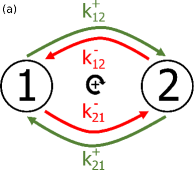
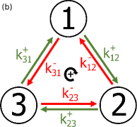
Figure 1: Small discrete-state cycles. (a) Two-state and (b) three-state cycles. Forward (clockwise, green) and reverse (counterclockwise, red) transitions occur along each pathway connecting two states, with respective rate constants $k_{ij}^{+}$ and $k_{ij}^{-}$.

A transition from state $i$ to state $j$ occurs at the forward rate $k_{ij}^{+}P_{i}$, with $P_{i}$ the probability in state $i$. Reverse transitions from state $j$ to state $i$ occur at rate $k_{ij}^{-}P_{j}$. (Note that the two-state cycle has both pathway 12 and pathway 21, representing distinguishable physical transition mechanisms, each with a forward and reverse direction.)

Typically, cellular cycles are driven by nonequilibrium concentrations of reacting chemical species, most prominently adenosine triphosphate (ATP), adenosine diphosphate (ADP), and inorganic phosphate ($\text{P}_{\text{i}}$) Phillips et al. (2012). The free energy $\Delta G$ provided by ATP hydrolysis depends on the respective concentrations Phillips et al. (2012),

$$\Delta G=\Delta G_{0}+k_{\text{B}}T\ln\frac{[\text{ADP}][\text{P}_{\text{i}}]}{[\text{ATP}]}\ ,$$ (1)

where $\Delta G_{0}\equiv-k_{\text{B}}T\ln\left([\text{ADP}]_{\text{eq}}[\text{P}_{\text{i}}]_{\text{eq}}/[\text{ATP}]_{\text{eq}}\right)$, $k_{\text{B}}$ is Boltzmann’s constant, and $T$ is the temperature of the surrounding environment. Under physiological conditions, hydrolysis of ATP to ADP and $\text{P}_{\text{i}}$ provides free energy $|\Delta G|\sim 20k_{\text{B}}T$ Phillips et al. (2012). From here on we set $k_{\text{B}}T=1$ — all free energies are in units of the thermal energy scale.

The ratio between the forward and reverse rate constants of a given transition path is fixed by its free energy dissipation $\omega_{ij}$  Wagoner and Dill (2016); Pietzonka et al. (2016),

$$\omega_{ij}=\ln\frac{k_{ij}^{+}}{k_{ij}^{-}}\ .$$ (2)

(See Appendix.) Without a bias $\omega_{ij}$, the full forward and reverse rate constants $k_{ij}^{+/-}$ equal the ‘bare’ rate constants $k_{ij}^{0}$.

II.2 Free energy landscape

A discrete-state kinetic model of a machine cycle can also be equivalently represented by Arrhenius dynamics on a free energy landscape, with each free energy well representing a discrete state, and the free energy differences between barriers (at energies $E_{ij}^{\ddagger}$) and states (at energies $E_{i}$) determining the rate constants,

$$k_{ij}^{+}=\tau_{ij}^{-1}e^{-(E^{\ddagger}_{ij}-E_{i})}\ \ \text{and}\ \ k_{ij}^{-}=\tau_{ij}^{-1}e^{-(E^{\ddagger}_{ij}-E_{j})}\ ,$$ (3)

with $\tau_{ij}$ a timescale accounting for effective diffusivity. The free energy budget $\omega_{\text{tot}}$ fixes the free energy difference between equivalent molecular machine states separated by one cycle. For example, Fig. 2 represents a two-state cycle, with dissipations $\omega_{12}=E_{1}-E_{2}$, and $\omega_{21}=E_{2}-(E_{1}-\omega_{\text{tot}})$.

The bare rates $k_{ij}^{0}$ are the rates in the absence of chemical driving. We restrict our attention to wells at equal free energy without chemical driving, so forward and reverse bare rates of a given transition are equal. We allow bare rates to vary among the different transitions to account for differences in barrier heights, effective diffusivity, and all other dissipation-independent factors.

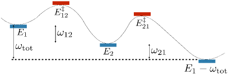
Figure 2: Free energy landscape representing a two-state molecular machine. The left-most state (at free energy $E_{1}$) and the right-most state ($E_{1}-\omega_{\text{tot}}$) represent the same stage of molecular machine operation, separated by one complete cycle. The middle state ($E_{2}$) represents an intermediate state, while $E^{\ddagger}_{12}$ and $E^{\ddagger}_{21}$ are the free energies of barriers between the states. $\omega_{12}$ and $\omega_{21}$ are the dissipations for each transition, which sum to $\omega_{\text{tot}}$, the dissipation budget for one cycle.

III Results

We maximize the steady-state flux by allocating a fixed free energy budget $\omega_{\text{tot}}$ among the free energy differences $\omega_{ij}$ between discrete states (i.e. dissipation over discrete transitions), which determines the full rate constants $k_{ij}^{+/-}$ and hence the net steady-state flux $J$ (from here on, the flux), which for a two-state cycle is Hill (1977)

$$J=\frac{k_{12}^{+}k_{21}^{+}-k_{12}^{-}k_{21}^{-}}{k_{12}^{+}+k_{12}^{-}+k_{21}^{+}+k_{21}^{-}}\ .$$ (4)

We first consider freely varying $E_{2}$, $E^{\ddagger}_{12}$, and $E^{\ddagger}_{21}$ (see Fig. 2). When barriers are higher than states, decreasing the barrier energies always increases flux,

$$\frac{\partial J}{\partial E^{\ddagger}_{12}}<0\ \ \text{and}\ \ \frac{\partial J}{\partial E^{\ddagger}_{21}}<0\ .$$ (5)

(See Appendix for details.) Flux is maximized when the ‘barriers’ are at or below the states, thus no longer acting as barriers. This is an intuitive result, that all else equal, faster transitions (due to lowered barriers) produce a higher flux Wagoner and Dill (2016).

Increasing $E_{2}$ is equivalent to decreasing the dissipation $\omega_{12}$ and increasing $\omega_{21}$, and vice versa. For fixed barrier energies $E^{\ddagger}_{12}$ and $E^{\ddagger}_{21}$, flux is maximized by increasing $E_{2}$ above the free energy of one of the barriers, effectively producing a one-state cycle (see Appendix).

Transition rates are reduced by energetic barriers, so flux is maximized by removing barriers and reducing the number of metastable states. However, a greater number of metastable states, each representing a persistent conformation or ligand binding status of a biomolecular machine, make possible a larger array of schemes for the following: interaction, such as distinct binding affinities Mason et al. (1999); machine operation, such as ‘gating’ Dogan et al. (2015); and regulation through variable action on distinct states Huse and Kuriyan (2002).

Multiple metastable states can be maintained by constraining the free energy landscape to preserve barriers. We implement these constraints by fixing the free energy differences between wells and either the barriers immediately before or immediately after them, equivalent to fixing the rate constants between discrete states for either the forward or reverse transitions. A forward labile (FL) scheme (case A in Thomas et al. (2001)) keeps the reverse free energy differences fixed, with the dissipation $\omega_{ij}$ only modifying the forward rate constant,

$$k_{ij}^{+}=k_{ij}^{0}e^{\omega_{ij}}\ \ \text{and}\ \ k_{ij}^{-}=k_{ij}^{0}\ ;$$ (6)

whereas for a reverse labile (RL) scheme (case B in Thomas et al. (2001)), the dissipation only modifies the reverse rate constant,

$$k_{ij}^{+}=k_{ij}^{0}\ \ \text{and}\ \ k_{ij}^{-}=k_{ij}^{0}e^{-\omega_{ij}}\ .$$ (7)

For the free energy landscape of Fig. 2, the FL scheme has fixed $E^{\ddagger}_{12}-E_{2}$ and $E^{\ddagger}_{21}-(E_{1}-\omega_{\text{tot}})$, while the RL scheme has fixed $E^{\ddagger}_{12}-E_{1}$ and $E^{\ddagger}_{21}-E_{2}$.

‘Labile’ here denotes the direction in which rate constants change with dissipation. This dependence of forward or reverse rate constants on dissipation for the FL and RL schemes, respectively, is analogous to their dependence on the work performed by a motor in a ‘power stroke’ or ‘Brownian ratchet’ Wagoner and Dill (2016).

III.1 Forward Labile Scheme

III.1.1 Two-state cycle

For a two-state FL cycle (Fig. 1a) with fixed total cycle dissipation $\omega_{\text{tot}}=\omega_{12}+\omega_{21}$, flux (Eq. (4)) is maximized when the free energy dissipation of the first transition is

$$\omega^{*}_{12}=\frac{1}{2}\omega_{\text{tot}}+\frac{1}{2}\ln\frac{k_{21}^{0}}{k_{12}^{0}}\ .$$ (8)

This produces equal forward rate constants,

$$k_{ij}^{+}=\sqrt{k_{12}^{0}k_{21}^{0}}\ e^{\omega_{\text{tot}}/2}\ ,$$ (9)

equal to the geometric mean of any full rate constants $k_{12}^{+}$ and $k_{21}^{+}$ consistent with the bare rate constants $k_{ij}^{0}$ and total dissipation $\omega_{\text{tot}}$.

The optimal allocation of total dissipation $\omega_{\text{tot}}$ differs from the ‘naive’ allocation $\frac{1}{2}\omega_{\text{tot}}$ that evenly divides the dissipation among the transitions. More specifically, the optimal deviation from the naive allocation is $\Delta\omega^{*}_{12}\equiv\omega^{*}_{12}-\frac{1}{2}\omega_{\text{tot}}=\tfrac{1}{2}\ln(k_{21}^{0}/k_{12}^{0})$. The optimal allocation compensates for variation in bare rate constants, so for FL, transitions with larger $k_{ij}^{0}$ are optimally allocated less dissipation. In fact, the optimal allocation of dissipation to one transition is negative when $|\ln(k_{21}^{0}/k_{12}^{0})|>\omega_{\text{tot}}$.

III.1.2 Three-state cycle

For a three-state cycle (Fig. 1b), the flux is Hill (1977)

$$J=\dfrac{k_{12}^{+}k_{23}^{+}k_{31}^{+}-k_{12}^{-}k_{23}^{-}k_{31}^{-}}{\left(\displaystyle\begin{multlined}k_{12}^{+}k_{23}^{-}+k_{12}^{-}k_{23}^{-}+k_{23}^{-}k_{31}^{-}+k_{12}^{+}k_{31}^{+}+k_{12}^{-}k_{31}^{+}\\ +k_{12}^{-}k_{31}^{-}+k_{12}^{+}k_{23}^{+}+k_{23}^{+}k_{31}^{+}+k_{23}^{+}k_{31}^{-}\end{multlined}k_{12}^{+}k_{23}^{-}+k_{12}^{-}k_{23}^{-}+k_{23}^{-}k_{31}^{-}+k_{12}^{+}k_{31}^{+}+k_{12}^{-}k_{31}^{+}\\ +k_{12}^{-}k_{31}^{-}+k_{12}^{+}k_{23}^{+}+k_{23}^{+}k_{31}^{+}+k_{23}^{+}k_{31}^{-}\right)}\ .$$ (10)

For FL, Fig. 3 shows the numerically determined allocation of free energy dissipation that maximizes the flux subject to a fixed $\omega_{\text{tot}}=\omega_{12}+\omega_{23}+\omega_{31}$ and fixed second and third bare rate constants $k_{23}^{0}=k_{31}^{0}=1$, for several different $k_{12}^{0}$ across multiple orders of magnitude Hwang and Hyeon (2017). When $k_{12}^{0}=1$, the $\omega^{*}_{ij}$ all equal the naive value $\frac{1}{3}\omega_{\text{tot}}$, as expected by symmetry. As $k_{12}^{0}$ increases, the optimal allocations $\omega^{*}_{ij}$ depart from the naive case, with the dissipation $\omega^{*}_{12}$ of the first transition decreasing, and that of the second and third transitions ($\omega^{*}_{23}$ and $\omega^{*}_{31}$) increasing.

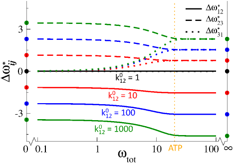
Figure 3: Uneven allocation of dissipation maximizes flux in a three-state forward labile cycle. Dissipation allocations $\Delta\omega^{*}_{12}$ (solid curves), $\Delta\omega^{*}_{23}$ (dashed), and $\Delta\omega^{*}_{31}$ (dotted) for the three transitions in Fig. 1b that maximize the flux. Dissipations expressed as differences $\Delta\omega^{*}_{ij}\equiv\omega^{*}_{ij}-\frac{1}{3}\omega_{\text{tot}}$ from the naive allocation of equal dissipation $\tfrac{1}{3}\omega_{\text{tot}}$ to each transition. $k_{23}^{0}=k_{31}^{0}=1$ is fixed, and $k_{12}^{0}$ varies with color. When $k_{12}^{0}=1$ (black), an even allocation of dissipation to each transition maximizes flux, so $\Delta\omega^{*}_{ij}=0$ for all $\omega_{\text{tot}}$. As $k_{12}^{0}$ increases (black$\to$red$\to$blue$\to$green), the flux-maximizing allocation increasingly deviates from an even allocation, as shown by the increasing magnitude of $\Delta\omega^{*}_{ij}$. Allocations at limiting $\omega_{\text{tot}}$ are shown by circles (low $\omega_{\text{tot}}$ plotted at $\omega_{\text{tot}}=0$, Eq. (11); high $\omega_{\text{tot}}$ at $\omega_{\text{tot}}=\infty$, Eq. (13)). Vertical dotted orange line at $\omega_{\text{tot}}=20$ represents the ATP hydrolysis free energy under physiological conditions.

At high $\omega_{\text{tot}}$, the reverse flux is much smaller than the forward flux, $J_{ij-}=k_{ij}^{-}P_{j}\ll k_{ij}^{+}P_{i}=J_{ij+}$, and hence the net flux roughly equals the forward flux, $J=J_{ij+}-J_{ij-}\simeq J_{ij+}$. In this limit, the cycle effectively only has forward transitions, leading (see Appendix) to an optimal dissipation allocation

$$\Delta\omega^{*}_{12}=\frac{1}{3}\ln\frac{k_{23}^{0}k_{31}^{0}}{\left(k_{12}^{0}\right)^{2}}$$ (11)

that is independent of $\omega_{\text{tot}}$. Similar expressions for $\Delta\omega_{23}^{*}$ and $\Delta\omega_{31}^{*}$ are found by cyclically permuting the indices in Eq. (11). These asymptotic values (Fig. 3, circles on the right edge) are indistinguishable from the limits of the numerical calculations. This optimal dissipation allocation produces equal forward rate constants

$$k_{ij}^{+}=k_{ij}^{0}e^{\omega_{ij}}=(k_{12}^{0}k_{23}^{0}k_{31}^{0}e^{\omega_{\text{tot}}})^{1/3}\ ,$$ (12)

that are the geometric mean of any full rate constants $k_{12}^{+}$, $k_{23}^{+}$, and $k_{31}^{+}$, consistent with $k_{ij}^{0}$ and $\omega_{\text{tot}}$.

At low $\omega_{\text{tot}}$, when the net flux $J=J_{ij+}-J_{ij-}$ is much smaller than either the forward or reverse fluxes, $J\ll J_{ij+}$ and $J\ll J_{ij-}$, the optimal $\omega_{ij}$ also asymptotically approach (generally nonzero) values independent of $\omega_{\text{tot}}$. Maximizing the net flux in Eq. (10) at low $\omega_{\text{tot}}$ leads (see Appendix) to an optimal allocation

$$\omega_{12}^{*}=\frac{1}{2}\ln\frac{k_{31}^{0}}{k_{12}^{0}}\ .$$ (13)

Similar expressions for $\omega^{*}_{23}$ and $\omega^{*}_{31}$ are found by cyclically permuting the indices in Eq. (13). These asymptotic values (Fig. 3, circles on the left edge) show excellent agreement with the limiting numerical calculations.

At high total dissipation $\omega_{\text{tot}}$, the optimal allocation $\omega^{*}_{ij}$ reaches a limit where for all transitions the forward rates are much larger than the reverse rates, becoming effectively irreversible. For the three-state cycle, the 20$k_{\text{B}}T$ of free energy provided by ATP hydrolysis is near this limit (Fig. 3). However, not all transitions will be effectively irreversible for a smaller dissipation budget per cycle step, which is obtained for machines that perform work against a resistive load or machines with more states per cycle.

The results above demonstrate that the optimal allocation of dissipation can significantly differ from an equal allocation to each transition. Fig. 4 shows the variation of flux as the dissipation allocation is varied away from the optimal allocation. Exploring a range of several $k_{\rm B}T$ around the optimal allocation, the flux varies by more than three orders of magnitude. Thus a dissipation allocation significantly different from the optimal one can qualitatively alter the cycle output.

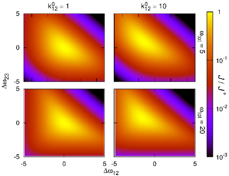
Figure 4: Flux is sensitive to dissipation allocation. Flux ratio $J/J^{*}$ as a function of the dissipation allocation, for the three-state forward labile cycle with $k_{23}^{0}=k_{31}^{0}=1$, and $k_{12}^{0}$ and $\omega_{\text{tot}}$ varying across subplots. Dissipation allocations are shown as differences $\Delta\omega_{ij}\equiv\omega_{ij}-\tfrac{1}{3}\omega_{\text{tot}}$ from naive values $\tfrac{1}{3}\omega_{\text{tot}}$. Optimal flux $J^{*}$ is specific to each subplot.

III.2 Reverse Labile Scheme

For a two-state RL cycle (as opposed to a FL cycle), the flux-maximizing allocation of dissipation is (Appendix)

$$\Delta\omega^{*}_{12}=-\frac{1}{2}\ln\frac{k_{21}^{0}}{k_{12}^{0}}\ .$$ (14)

The deviations in Eq. (14) from naive allocations are identical to the FL result (Eq. (8)), except assigned to the other transition. Despite this apparent difference, in each state the probability that the next transition will move in the forward or reverse direction (and hence the ratio of one-sided fluxes) is identical for the optimized FL and RL cycles. For example, both schemes produce one-sided fluxes departing from state 1 that satisfy (see Appendix)

$$\frac{J^{*}_{12+}}{J^{*}_{21-}}=\sqrt{\frac{k_{12}^{0}}{k_{21}^{0}}}e^{\omega_{\text{tot}}/2}\ .$$ (15)

Similarly, for the three-state cycle, both mechanisms allocate dissipation identically, except cyclically permuted (Fig. 5a). Thus optimal dissipation allocation in the three-state cycle also produces one-sided flux ratios that do not depend on the mechanism. The limiting optimal allocations at high $\omega_{\text{tot}}$ are (Appendix)

$$\Delta\omega_{12}^{*}=\frac{1}{3}\ln\frac{k_{12}^{0}k_{31}^{0}}{\left(k_{23}^{0}\right)^{2}}\ ,$$ (16)

and at low $\omega_{\text{tot}}$ are (Appendix)

$$\omega^{*}_{12}=\frac{1}{2}\ln\frac{k_{12}^{0}}{k_{23}^{0}}\ .$$ (17)

These results are intuitive: an RL scheme can adjust reverse but not forward rates, and so to maximize the flux it allocates more dissipation to decelerate the fastest reverse rates (those with high $k_{ij}^{0}$); whereas an FL scheme can adjust forward but not reverse rates, so it allocates more dissipation to accelerate the slowest forward rates (with low $k_{ij}^{0}$).

Figure 5b shows the dependence of three-state RL flux on the dissipation allocation. For low $\omega_{\text{tot}}$ the flux varies substantially (by orders of magnitude) across allocations that differ by a few $k_{\rm B}T$ (similar to FL in Fig. 4), but at high $\omega_{\text{tot}}$ there is little variation of flux with dissipation allocation. The RL flux is less sensitive to the dissipation allocation at high $\omega_{\text{tot}}$ because once reverse rates are sufficiently suppressed to be negligible (i.e., for $e^{-\omega_{\text{tot}}/3}\ll 1$), reallocation of dissipation has reduced effect.

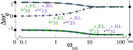
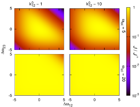
Figure 5: Optimal and sub-optimal allocations of dissipation for reverse labile scheme. (a) Allocation of dissipation $\omega_{ij}$ to maximize flux around the three-state cycle, for forward labile (green) and reverse labile (purple) schemes. The optimal dissipation values are identical for the two mechanisms (as illustrated by the overlapping green and purple curves on the plot), however the individual dissipations are allocated to different transitions. Circles on the left and right edges show limiting optimal allocations at low and high total dissipation $\omega_{\text{tot}}$ (Eq. (17) and Eq. (16)), respectively. $k_{12}^{0}=10$ and $k_{23}^{0}=k_{31}^{0}=1$. (b) Flux sensitivity to dissipation allocation, analogous to Fig. 4, except for reverse labile scheme instead of forward labile.

For given bare rates $k_{ij}^{0}$ and total dissipation $\omega_{\text{tot}}$, an FL cycle will always produce more flux than the corresponding RL cycle, similar to previous results Wagoner and Dill (2016). FL and RL schemes represent extremes of a more general mechanism, whereby some dissipation is spent speeding up the forward transitions (as for FL), and the remaining fraction slows down the reverse transitions (as for RL):

$$k_{ij}^{+}=k_{ij}^{0}e^{\omega_{ij}^{+}}\ \ \text{and}\ \ k_{ij}^{-}=k_{ij}^{0}e^{-\omega_{ij}^{-}}\ .$$ (18)

This is similar to splitting force-dependence among reaction rates in previous studies Fisher and Kolomeisky (1999); Wagoner and Dill (2016). $\sum(\omega_{ij}^{+}+\omega_{ij}^{-})=\omega_{\text{tot}}$ is fixed, leaving $2n-1$ free parameters to optimize over in an $n$-state cycle. For any given dissipation allocation, flux can always be increased by shifting some dissipation $\delta\omega$ from slowing the reverse rate to speeding the corresponding forward rate. This is equivalent to simply lowering the barriers for the free energy landscape in Fig. 2, which removes the distinction between states, as discussed above.

IV Discussion

The Second Law of thermodynamics requires free energy dissipation to break detailed balance and maintain directed flux  Machta (2015), but does not specify a quantitative relationship between dissipation and flux Barato and Seifert (2015); Feng and Crooks (2008); Brown and Sivak (2016).

From the perspective of a free energy landscape, we find that the flux is increased by lowering the barriers so that they are no longer effective. This is intuitive, as transition rates are reduced by energetic barriers, and suggests that molecular machines should reduce the number of metastable states to increase forward flux. However, molecular machines perform their tasks using multiple metastable states, and accordingly we have focused on scenarios that allow distinct states to be maintained.

In a reaction cycle with a fixed number of discrete states, we have shown that flux is maximized by an uneven allocation of a fixed dissipation budget among the various discrete transitions, compensating for differences in the bare rate constants of each transition (see Eq. (8) and Eq. (14), Figs. 3 and 5a). This is related to recent findings that flux is affected differently by adjusting the bare rate of different transitions Wagoner and Dill (2016). The flux can be quite sensitive to the precise dissipation allocation (Figs. 4 and 5b), suggesting a significant cost to non-optimal allocations.

This result differs from the uniform allocations found to be optimal in various other contexts, including maximizing power at fixed entropy production rate Qian et al. (2016), minimizing entropy production at fixed flux Qian (2000); Sauar et al. (1996); Johannessen and Kjelstrup (2005), maximizing free energy conversion efficiency Oster and Wang (2000), and minimizing the dissipation cost of a given precision Barato and Seifert (2015). Several other studies have argued that to maintain a high flux, large free energy increases should be broken up into smaller pieces, with no individual free energy change too large Hill and Eisenberg (1981); Yu et al. (2007); Anandakrishnan et al. (2016). Even in synthetic molecular motors, it is thought that similar forward rates are optimal (to avoid ‘traffic jams’) Geertsema et al. (2009).

We find an unequal optimal dissipation allocation occurs when: the nonequilibrium steady-state flux is maximized ; optimization is subject to fixed total dissipation budget per cycle ; the ratio of forward and reverse rate constants varies exponentially, not linearly, with dissipation (Eq. (2)); and cycle transitions have different bare rate constants, corresponding to different barrier heights and effective diffusivities. For some previous studies finding even dissipation allocations to be optimal, a single change is sufficient to make uneven allocations optimal: e.g., imposing distinct bare rate constants Barato and Seifert (2015) or changing the dependence of flux on dissipation from linear (the near-equilibrium case) to exponential Sauar et al. (1996).

Many models parametrized to biomolecular machine dynamics contain effectively irreversible transitions, e.g., models of kinesin Clancy et al. (2011); Visscher et al. (1999), myosin Cappello et al. (2007); Xie et al. (2006), RNA polymerase Abbondanzieri et al. (2005), and viral packaging motors Moffitt et al. (2009); Liu et al. (2014). Such irreversible transitions are, strictly speaking, unphysical due to their violation of microscopic reversibility Fisher and Kolomeisky (1999); Astumian (2015); in reality they represent a forward rate constant much larger than the reverse rate constant, a signature of large dissipation over that transition. Since other transitions in these models are reversible, this implies the dissipation allocation in such models must be highly unequal, consistent with the uneven dissipation allocation we find maximizes flux.

Other models of driven biomolecular cycles—such as in myosin Fox (1998); Skau et al. (2006); Wu et al. (2007) and several enzymes Hwang and Hyeon (2017)—lack explicitly irreversible transitions, but have ratios of forward and reverse rate constants, and hence free energy dissipation, that vary significantly across the different reactions composing a cycle.

Dissipation biases forward and reverse rate constants, but there is no unique way to achieve this bias Thomas et al. (2001); Wagoner and Dill (2016). We explored in detail two extremes for how dissipation can lead to biased progress: a forward labile scheme, where dissipation increases forward rate constants; and a reverse labile scheme, where dissipation decreases reverse rate constants. Although FL and RL mechanisms lead to distinct optimal allocations of dissipation, both lead to identical transition probability ratios from each state (Eq. (15)). An FL cycle produces more flux than a comparable RL cycle, but FL flux is quite sensitive to the dissipation allocation (Fig. 4), while RL flux is insensitive to the dissipation allocation for a large free energy budget (Fig. 5b).

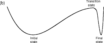
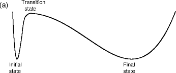
Figure 7: Correspondence between energy landscapes and forward and reverse labile schemes. Forward labile and reverse labile schemes use dissipation to change only forward and reverse rate constants, respectively. In analogy to force-induced unfolding Elms et al. (2012), the proximity of the transition state can lead to forward and reverse rates differing in their sensitivity to dissipation. (a) The forward labile scheme corresponds to a transition state quite close to the final state. Changes in the free energy difference between initial and final state (dissipation) lead to a change in the difference between initial and transition states, but not a significant change in the difference between the final and transition states. This changes the forward rate, but not the reverse. (b) Conversely, the reverse labile scheme corresponds to a transition state quite close to the initial state. Dissipation changes lead to relative changes between the final and transition states, but not the initial and transition states. This changes the reverse rate, but not the forward. These two scenarios are extremes; the transition state could be anywhere between the initial and final states.

On evolutionary timescales, mutations alter the conformational free energies of initial and final states differently. For a transition state conformationally similar to the initial state, a mutation should produce similar changes in the initial and transition state free energies, so the forward rate should change less than the backward rate. This is analogous to the distance to the transition state affecting the sensitivity of unfolding rates to applied force Elms et al. (2012). Our FL and RL mechanisms thus correspond to a transition state conformationally similar to the final and to the initial states, respectively (see Appendix, Fig. 7).

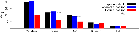
Figure 6: Forward labile predictions better match experimental dissipation allocations than do even allocations. Dissipation of transition $\omega_{12}$ in several enzymes, from fit to experiment (black) Hwang and Hyeon (2017), flux optimization under the FL scheme (blue), and even allocation (red). AP, alkaline phosphatase; TPI, triose phosphate isomerase. Details in Appendix.

Optimizing an FL cycle predicts that transitions with low bare rate constants will be allocated more dissipation, while for an RL cycle high bare rate constants are allocated more dissipation. Dissipation allocations for several two-state enzyme models Hwang and Hyeon (2017) fit to experiment are closely matched by the FL optimal allocation, generally much better than by an even allocation (Fig. 6) or the RL optimal allocation. See Appendix for more extensive comparisons.

We expect that adjusting the dissipation allocation (of a fixed total dissipation per cycle) would require only isolated changes in molecular machine dynamics, primarily affecting machine output or productivity, and minimally impacting the rest of the cell. In contrast, adjusting the dissipation budget, for example through the free energy of ATP hydrolysis, would affect numerous driven processes throughout the cell.

Adjustment of the dissipation allocation through isolated mutations is supported by experimental findings. Point mutations in the kinesin-1 nucleotide binding pocket likely affect the dissipation allocation by altering the size of the pocket Kapoor and Mitchison (1999) or the ADP unbinding rate Higuchi et al. (2004); Uchimura et al. (2010) and lead to significant decreases in kinesin velocity or ATP hydrolysis rate while remaining functional. Changes in binding affinity due to mutation (e.g., 2.5-fold change for a transcription regulator Huang et al. (2016), or 40-fold for a membrane regulatory protein Feig and Cooper (1988)) correspond to a different unbinding rate, which also would change the dissipation allocation.

Our optimizations omit several significant biophysical considerations. For example, we allow rate constants to vary without bound, although practically they are limited by molecular diffusion. We also focus on a single biomolecular cycle; an interesting extension would be to investigate the effects of alternative pathways thought to be present in biomolecular machines Clancy et al. (2011); Wu et al. (2007). Further elaborations of this work could explore the sensitivity of flux to (varying) resistive forces as well as cycle states vulnerable to ‘escape’ (such as a molecular motor falling off its track).

Appendix A Optimizations with varying number of metastable states

We investigate the free energy landscape of Fig. 2. For simplicity we set $E_{1}-\omega_{\text{tot}}=0$ and hence $E_{1}=\omega_{\text{tot}}$. The rate constants $k_{12}^{+/-}$ for forward and reverse transitions over the first barrier, with free energy $E^{\ddagger}_{12}$, are, respectively

$$k_{12}^{+}=\tau^{-1}_{12}e^{-(E^{\ddagger}_{12}-\omega_{\text{tot}})}\ \ \text{and}\ \ k_{12}^{-}=\tau^{-1}_{12}e^{-(E^{\ddagger}_{12}-E_{2})}\ .$$ (19)

The forward and reverse rate constants over the second barrier, with free energy $E^{\ddagger}_{21}$, are

$$k_{21}^{+}=\tau^{-1}_{21}e^{-(E^{\ddagger}_{21}-E_{2})}\ \ \text{and}\ \ k_{21}^{-}=\tau^{-1}_{21}e^{-E^{\ddagger}_{21}}\ .$$ (20)

The steady-state flux for a two-state cycle is Hill (1977)

$$J=\frac{k_{12}^{+}k_{21}^{+}-k_{12}^{-}k_{21}^{-}}{k_{12}^{+}+k_{12}^{-}+k_{21}^{+}+k_{21}^{-}}\ .$$ (21)

Inserting Eqs. (19) and (20) into (21) and rearranging gives

$$J=\frac{e^{\omega_{\text{tot}}}-1}{\tau_{12}e^{E^{\ddagger}_{12}}(1+e^{-E_{2}})+\tau_{21}e^{E^{\ddagger}_{21}}(1+e^{\omega_{\text{tot}}-E_{2}})}\ .$$ (22)

We consider the states at $E=\omega_{\text{tot}}$ and $E=0$ to be fixed, as varying them relative to one another changes the free energy budget $\omega_{\text{tot}}$. We vary $E_{2}$, $E^{\ddagger}_{12}$, and $E^{\ddagger}_{21}$ to maximize the flux $J$. Assuming barriers are higher than states, straightforward differentiation shows that

$$\frac{\partial J}{\partial E^{\ddagger}_{12}}<0\ \ \text{and}\ \ \frac{\partial J}{\partial E^{\ddagger}_{21}}<0\ ,$$ (23)

i.e., flux increases as either barrier height decreases. Once the barrier energies are at or below the neighboring state energies, Eqs. (19) and (20) no longer hold. Eq. (23) indicates that the flux is increased by removing the barriers altogether, leaving state 2 (at energy $E_{2}$) no longer metastable.

In a separate optimization, we constrain the barriers at fixed energies $E^{\ddagger}_{12}$ and $E^{\ddagger}_{21}$, and then vary $E_{2}$. Differentiating Eq. (22), again subject to barriers higher than states, gives

$$\frac{\partial J}{\partial E_{2}}>0\ ,$$ (24)

meaning that the flux increases as $E_{2}$ increases.

The previous two optimizations allowed either the barrier energies to decrease below the neighboring state energies, or $E_{2}$ to rise above the barrier energies. We now consider a scenario where the free energy differences $\Delta E_{12}^{-}=E^{\ddagger}_{12}-E_{2}$ and $\Delta E_{21}^{+}=E^{\ddagger}_{21}-E_{2}$ are fixed, so that $E_{2}$, $E^{\ddagger}_{12}$, and $E^{\ddagger}_{21}$ move up and down together. This gives rate constants

$$k_{12}^{+} =\tau^{-1}_{12}e^{-(E_{2}+\Delta E_{12}^{-}-\omega_{\text{tot}})}$$ (25a)

$$k_{12}^{-} =\tau^{-1}_{12}e^{-\Delta E_{12}^{-}}$$ (25b)

$$k_{21}^{+} =\tau^{-1}_{21}e^{-\Delta E_{21}^{+}}$$ (25c)

$$k_{21}^{-} =\tau^{-1}_{21}e^{-(E_{2}+\Delta E_{21}^{+})}\ .$$ (25d)

Substituting these rate constants into Eq. (21) gives

$$J=\frac{e^{\omega_{\text{tot}}}-1}{e^{E_{2}}(\tau_{12}e^{\Delta E_{12}^{-}}+\tau_{21}e^{\Delta E_{21}^{+}})+\tau_{12}e^{\Delta E_{12}^{-}}+\tau_{21}e^{\omega_{\text{tot}}+\Delta E_{21}^{+}}}\ .$$ (26)

When barriers are higher than states,

$$\frac{\partial J}{\partial E_{2}}<0\ ,$$ (27)

meaning the flux increases as $E_{2}$ decreases. This continues until one of the barriers is at or below one of the other two states, when Eq. (25) no longer holds. This optimization, similar to the previous two optimizations, increases the flux by removing the effect of the barriers.

Appendix B Additional model details

We describe our cycles with ‘basic’ free energy differences $\omega_{ij}$ Hill and Eisenberg (1981); Hill (1983), because they directly relate to the ratio of forward and reverse transition rate constants in Eq. (2). Unlike basic free energy differences, ‘gross’ free energy changes also include the entropic contribution associated with transitions between states with different occupation probabilities Hill (1983). At steady state, the entropic contributions included in the gross free energy cancel out over a complete cycle, making the basic and gross free energy budgets identical.

Appendix C Forward Labile Scheme

C.1 Two-state flux

For a two-state cycle, Eq. (21) gives the steady-state flux.

Each transition has a bare rate constant $k_{ij}^{0}$. The log-ratio of the full rate constants is the dissipation $\omega_{ij}$ of each transition, $k_{ij}^{+}/k_{ij}^{-}=e^{\omega_{ij}}$. For a forward labile scheme, dissipation increases the forward rate constant, $k_{ij}^{+}=k_{ij}^{0}e^{\omega_{ij}}$, and leaves unchanged the reverse rate constant $k_{ij}^{-}=k_{ij}^{0}$ (see main text). With these expressions, the flux can be rewritten as

$$J=\frac{k_{12}^{0}k_{21}^{0}\left(e^{\omega_{\text{tot}}}-1\right)}{k_{12}^{0}\left(e^{\omega_{12}}+1\right)+k_{21}^{0}\left(e^{\omega_{21}}+1\right)}\ .$$ (28)

We consider reaction cycles with a fixed total free energy dissipation $\omega_{\text{tot}}=\omega_{12}+\omega_{21}$. The dissipation allocation is determined by the single free parameter $\omega_{12}$, without loss of generality; the other transition’s dissipation $\omega_{21}=\omega_{\text{tot}}-\omega_{12}$ is then fixed. Setting $\text{d}J/\text{d}\omega_{12}=0$ gives

$$\omega^{*}_{12}=\frac{1}{2}\omega_{\text{tot}}+\frac{1}{2}\ln\frac{k_{21}^{0}}{k_{12}^{0}}\ .$$ (29)

The corresponding optimal flux is

$$J^{*}=\frac{k_{12}^{0}k_{21}^{0}(e^{\omega_{\text{tot}}}-1)}{k_{12}^{0}+k_{21}^{0}+2\sqrt{k_{12}^{0}k_{21}^{0}}e^{\omega_{\text{tot}}/2}}\ .$$ (30)

To quantify how $J/J^{*}$ decreases from 1 away from $\omega^{*}_{12}$, first we solve for $J/J^{*}$ near $\omega^{*}_{12}$. Differentiating Eq. (28) gives

$$\frac{\text{d}J}{\text{d}\omega_{12}}=\frac{k_{12}^{0}k_{21}^{0}(e^{\omega_{\text{tot}}}-1)(k_{21}^{0}e^{\omega_{\text{tot}}-\omega_{12}}-k_{12}^{0}e^{\omega_{12}})}{(k_{12}^{0}+k_{21}^{0}+k_{12}^{0}e^{\omega_{12}}+k_{21}^{0}e^{\omega_{\text{tot}}-\omega_{12}})^{2}}\ .$$ (31)

For $\omega_{12}=\omega^{*}_{12}+\delta$, expanding to first order in $\delta$ produces

$$\frac{\text{d}J}{\text{d}\omega_{12}}\simeq-\left(\frac{1}{2}\frac{k_{12}^{0}+k_{21}^{0}}{\sqrt{k_{12}^{0}k_{21}^{0}}}e^{-\omega_{\text{tot}}/2}+1\right)^{-1}\delta\ .$$ (32)

Integrating and rearranging gives, for small $|\delta|=|\omega_{12}-\omega^{*}_{12}|$,

$$\frac{J}{J^{*}}\simeq 1-\left(\frac{k_{12}^{0}+k_{21}^{0}}{\sqrt{k_{12}^{0}k_{21}^{0}}}e^{-\omega_{\text{tot}}/2}+2\right)^{-1}\delta^{2}\ .$$ (33)

For $J/J^{*}$ far from $\omega^{*}_{12}$, we divide Eq. (28) by Eq. (30),

$$\frac{J}{J^{*}}=\frac{k_{12}^{0}+k_{21}^{0}+2\sqrt{k_{12}^{0}k_{21}^{0}}e^{\omega_{\text{tot}}/2}}{k_{12}^{0}+k_{21}^{0}+k_{12}^{0}e^{\omega_{12}}+k_{21}^{0}e^{\omega_{\text{tot}}-\omega_{12}}}\ .$$ (34)

Rewriting $k_{12}^{0}e^{\omega_{12}}=\sqrt{k_{12}^{0}k_{21}^{0}}e^{\omega_{\text{tot}}/2}e^{\delta}$ and $k_{21}^{0}e^{\omega_{\text{tot}}-\omega_{12}}=\sqrt{k_{12}^{0}k_{21}^{0}}e^{\omega_{\text{tot}}/2}e^{-\delta}$ gives

$$\frac{J}{J^{*}}=\frac{k_{12}^{0}+k_{21}^{0}+2\sqrt{k_{12}^{0}k_{21}^{0}}e^{\omega_{\text{tot}}/2}}{k_{12}^{0}+k_{21}^{0}+\sqrt{k_{12}^{0}k_{21}^{0}}e^{\omega_{\text{tot}}/2}(e^{\delta}+e^{-\delta})}\ .$$ (35)

For large $|\delta|=|\omega_{12}-\omega^{*}_{12}|$,

$$\frac{J}{J^{*}}\simeq\left(\frac{k_{12}^{0}+k_{21}^{0}}{\sqrt{k_{12}^{0}k_{21}^{0}}}e^{-\omega_{\text{tot}}/2}+2\right)e^{-|\delta|}\ .$$ (36)

Fig. 8 compares Eqs. (33) and (36) to the exact $J/J^{*}$, showing good agreement in the expected regimes.

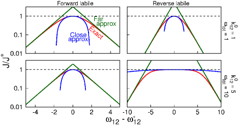
Figure 8: Two-state flux sensitivity. Flux ratio $J/J^{*}$ as a function of the dissipation allocation, for the two-state cycle with $k_{21}^{0}=1$, and $k_{12}^{0}$ and $\omega_{\text{tot}}$ as indicated. For forward labile (reverse labile) cycles, $J/J^{*}$ is given by Eqs. (28) and (30) ((44) and (45b)), the close approximation by Eq. (33) ((46)), and the far approximation by Eq. (36) ((47)). Dashed black line indicates $J/J^{*}=1$.

C.2 Three-state flux for high $\omega_{\text{tot}}$

For high total dissipation $\omega_{\text{tot}}$, the forward rate constants are exponentially increased, and the backward rate constants are negligible in comparison, producing a cycle with effectively only forward rates. A three-state cycle with only forward rates has steady-state probabilities

$$P_{1}^{\text{ss}}=\left[\left(k_{12}^{0}\right)^{-1}+\left(k_{23}^{0}\right)^{-1}e^{\omega_{12}-\omega_{23}}+\left(k_{31}^{0}\right)^{-1}e^{\omega_{12}-\omega_{31}}\right]^{-1}\ ,$$ (37)

with cyclic permutation of states giving $P_{2}^{\text{ss}}$ and $P_{3}^{\text{ss}}$. The resulting steady-state flux is

$$J=\left[\left(k_{12}^{0}e^{\omega_{12}}\right)^{-1}+\left(k_{23}^{0}e^{\omega_{23}}\right)^{-1}+\left(k_{31}^{0}e^{\omega_{31}}\right)^{-1}\right]^{-1}\ .$$ (38)

Solving for $\partial J/\partial\omega_{12}=\partial J/\partial\omega_{23}=0$ gives the optimal allocation

$$\omega^{*}_{12} =\frac{1}{3}\omega_{\text{tot}}+\frac{1}{3}\ln\frac{k_{23}^{0}k_{31}^{0}}{\left(k_{12}^{0}\right)^{2}}\ ,$$ (39a)

$$\omega^{*}_{23} =\frac{1}{3}\omega_{\text{tot}}+\frac{1}{3}\ln\frac{k_{31}^{0}k_{12}^{0}}{\left(k_{23}^{0}\right)^{2}}\ ,$$ (39b)

$$\omega^{*}_{31} =\frac{1}{3}\omega_{\text{tot}}+\frac{1}{3}\ln\frac{k_{12}^{0}k_{23}^{0}}{\left(k_{31}^{0}\right)^{2}}\ .$$ (39c)

C.3 Three-state flux for low $\omega_{\text{tot}}$

Substituting forward labile rate constants into Eq. (10) and solving for $\partial J/\partial\omega_{12}=\partial J/\partial\omega_{23}=0$, subject to fixed $\omega_{\text{tot}}=\omega_{12}+\omega_{23}+\omega_{31}$, gives

$$e^{2\omega^{*}_{12}} =k_{31}^{0}\frac{(k_{12}^{0})^{-1}+(k_{23}^{0})^{-1}e^{-\omega^{*}_{23}}}{1+e^{\omega^{*}_{23}}}e^{\omega_{\text{tot}}}\ ,$$ (40a)

$$e^{2\omega^{*}_{23}} =\frac{1}{k_{23}^{0}}\frac{1+e^{-\omega^{*}_{12}}}{(k_{12}^{0})^{-1}+(k_{31}^{0})^{-1}e^{\omega^{*}_{12}}}e^{\omega_{\text{tot}}}\ .$$ (40b)

For small $\omega_{\text{tot}}$, $e^{\omega_{\text{tot}}}\simeq 1$, giving

$$e^{2\omega^{*}_{12}} =k_{31}^{0}\frac{(k_{12}^{0})^{-1}+(k_{23}^{0})^{-1}e^{-\omega^{*}_{23}}}{1+e^{\omega^{*}_{23}}}\ ,$$ (41a)

$$e^{2\omega^{*}_{23}} =\frac{1}{k_{23}^{0}}\frac{1+e^{-\omega^{*}_{12}}}{(k_{12}^{0})^{-1}+(k_{31}^{0})^{-1}e^{\omega^{*}_{12}}}\ .$$ (41b)

Substituting Eq. (41b) into Eq. (41a) gives

$$\omega^{*}_{12}=\frac{1}{2}\ln\frac{k_{31}^{0}}{k_{12}^{0}}\ .$$ (42)

Similar derivations yield

$$\omega^{*}_{23}=\frac{1}{2}\ln\frac{k_{12}^{0}}{k_{23}^{0}}\ ,$$ (43a)

$$\omega^{*}_{31}=\frac{1}{2}\ln\frac{k_{23}^{0}}{k_{31}^{0}}\ .$$ (43b)

Appendix D Reverse Labile Scheme

D.1 Two-state flux

Given rate constants $k_{ij}^{+}$ and $k_{ij}^{-}$, the steady-state flux is Eq. (21). Substituting reverse labile rate constants $k_{ij}^{+}=k_{ij}^{0}$ and $k_{ij}^{-}=k_{ij}^{0}e^{-\omega_{ij}}$ gives

$$J=\frac{1-e^{-\omega_{\text{tot}}}}{(k_{21}^{0})^{-1}\left(1+e^{-\omega_{12}}\right)+(k_{12}^{0})^{-1}\left(1+e^{-\omega_{21}}\right)}\ .$$ (44)

Solving $\text{d}J/\text{d}\omega_{12}=0$ subject to fixed $\omega_{\text{tot}}=\omega_{12}+\omega_{21}$ gives

$$\omega^{*}_{12} =\frac{1}{2}\omega_{\text{tot}}-\frac{1}{2}\ln\frac{k_{21}^{0}}{k_{12}^{0}}$$ (45a)

$$J^{*} =\frac{1-e^{-\omega_{\text{tot}}}}{(k_{12}^{0})^{-1}+(k_{21}^{0})^{-1}+2(k_{12}^{0}k_{21}^{0}e^{\omega_{\text{tot}}})^{-1/2}}\ .$$ (45b)

Following similar steps as in Section C.1, we find for small $|\delta|=|\omega_{12}-\omega^{*}_{12}|$,

$$\frac{J}{J^{*}}\simeq 1-\left(\frac{k_{12}^{0}+k_{21}^{0}}{\sqrt{k_{12}^{0}k_{21}^{0}}}e^{\omega_{\text{tot}}/2}+2\right)^{-1}\delta^{2}\ ,$$ (46)

and for large $|\delta|=|\omega_{12}-\omega^{*}_{12}|$,

$$\frac{J}{J^{*}}\simeq\left(\frac{k_{12}^{0}+k_{21}^{0}}{\sqrt{k_{12}^{0}k_{21}^{0}}}e^{\omega_{\text{tot}}/2}+2\right)e^{-|\delta|}\ .$$ (47)

Fig. 8 compares Eqs. (46) and (47) to exact $J/J^{*}$, showing good agreement in the expected regimes.

For the two-state cycle, $\omega^{*,\text{FL}}_{12}=\omega^{*,\text{RL}}_{21}$ and $\omega^{*,\text{FL}}_{21}=\omega^{*,\text{RL}}_{12}$. This gives

$$\frac{J_{12+}^{*,\text{FL}}}{J_{21-}^{*,\text{FL}}} =\frac{k_{12}^{0}}{k_{21}^{0}}e^{\omega^{*,\text{FL}}_{12}}\ ,$$ (48a)

$$\frac{J_{12+}^{*,\text{RL}}}{J_{21-}^{*,\text{RL}}} =\frac{k_{12}^{0}}{k_{21}^{0}}e^{\omega^{*,\text{RL}}_{21}}\ .$$ (48b)

Substituting $\omega^{*,\text{FL}}_{12}=\omega^{*,\text{RL}}_{21}$ gives

$$\frac{J_{12+}^{*,\text{FL}}}{J_{21-}^{*,\text{FL}}}=\frac{J_{12+}^{*,\text{RL}}}{J_{21-}^{*,\text{RL}}}\ .$$ (49)

Because $\omega^{*,\text{FL}}_{12}=\frac{1}{2}\omega_{\text{tot}}+\frac{1}{2}\ln(k_{21}^{0}/k_{12}^{0})$, the ratios in Eq. (49) are $\sqrt{k_{12}^{0}/k_{21}^{0}}e^{\omega_{\text{tot}}/2}$.

D.2 Three-state flux for high $\omega_{\text{tot}}$

Substituting reverse labile rate constants into Eq. (10) and solving for $\partial J/\partial\omega_{12}=\partial J/\partial\omega_{23}=0$, subject to fixed $\omega_{\text{tot}}=\omega_{12}+\omega_{23}+\omega_{31}$, gives

$$e^{-2\omega^{*}_{12}} =\frac{1}{k_{12}^{0}}\frac{1+e^{\omega^{*}_{23}}}{(k_{23}^{0})^{-1}+(k_{31}^{0})^{-1}e^{-\omega^{*}_{23}}}e^{-\omega_{\text{tot}}}\ ,$$ (50a)

$$e^{-2\omega^{*}_{23}} =k_{31}^{0}\frac{(k_{23}^{0})^{-1}+(k_{12}^{0})^{-1}e^{\omega^{*}_{12}}}{1+e^{-\omega^{*}_{12}}}e^{-\omega_{\text{tot}}}\ .$$ (50b)

For high $\omega_{\text{tot}}$, these two equations are satisfied by

$$\omega^{*}_{12}=\frac{1}{3}\omega_{\text{tot}}+\frac{1}{3}\ln\frac{k_{12}^{0}k_{31}^{0}}{\left(k_{23}^{0}\right)^{2}}\ .$$ (51)

D.3 Three-state flux for low $\omega_{\text{tot}}$

Approximating $e^{-\omega_{\text{tot}}}\simeq 1$ in Eqs. (50a) and (50b) gives

$$e^{-2\omega^{*}_{12}} =\frac{1}{k_{12}^{0}}\frac{1+e^{\omega^{*}_{23}}}{(k_{23}^{0})^{-1}+(k_{31}^{0})^{-1}e^{-\omega^{*}_{23}}}\ ,$$ (52a)

$$e^{-2\omega^{*}_{23}} =k_{31}^{0}\frac{(k_{23}^{0})^{-1}+(k_{12}^{0})^{-1}e^{\omega^{*}_{12}}}{1+e^{-\omega^{*}_{12}}}\ .$$ (52b)

Substituting Eq. (52b) into Eq. (52a) gives

$$\omega^{*}_{12}=\frac{1}{2}\ln\frac{k_{12}^{0}}{k_{23}^{0}}\ .$$ (53)

Appendix E Experimentally parameterized models

Table 1 shows Hwang and Hyeon’s Hwang and Hyeon (2017) two-state parameterization of the forward and reverse rate constants for catalase, urease, alkaline phosphatase (AP), triose phosphate isomerase (TPI), and kinesin. The dissipation allocation $\omega_{12}$ and $\omega_{21}$ from these rate constants is compared to the optimal dissipation allocations predicted for forward labile cycles, $\omega_{ij}^{*,\text{FL}}$, and reverse labile cycles, $\omega_{ij}^{*,\text{RL}}$. Fig. 6 summarizes the comparison of experimental fit, forward labile prediction, and even allocation.

	Catalase	Urease	AP	TPI	Kinesin
$k_{12}^{+}$	$5.8\times 10^{4}$	$1.7\times 10^{4}$	$1.5\times 10^{5}$	$1.7\times 10^{5}$	$2.2\times 10^{3}$
$k_{12}^{-}$	$2.2\times 10^{-13}$	$7.4\times 10^{-7}$	$4\times 10^{-4}$	$4.2\times 10^{3}$	$5.5\times 10^{-1}$
$k_{21}^{+}$	$6.2\times 10^{6}$	$3\times 10^{5}$	$1.6\times 10^{5}$	$1.8\times 10^{5}$	$9.9\times 10^{1}$
$k_{21}^{-}$	$6.1\times 10^{6}$	$2.8\times 10^{5}$	$1.4\times 10^{4}$	$1.3\times 10^{4}$	$9.2\times 10^{-2}$
$\omega_{12}$	$40$	$24$	$20$	$3.7$	$8.3$
$\omega_{12}^{\text{even}}$	$20$	$12$	$10$	$3.2$	$7.7$
$\omega_{12}^{*,\text{FL}}$	$42.4$	$25.3$	$18.6$	$3.7$	$6.6$
$\omega_{12}^{*,\text{RL}}$	$17.7$	$6.6$	$7.5$	$2.6$	$9.1$
$\omega_{21}$	$0.02$	$0.07$	$0.13$	$2.6$	$7$
$\omega_{21}^{\text{even}}$	$20$	$12$	$10$	$3.2$	$7.7$
$\omega_{21}^{*,\text{FL}}$	$-2.4$	$-1.3$	$-1.2$	$2.6$	$8.4$
$\omega_{21}^{*,\text{RL}}$	$22.3$	$13.4$	$9.9$	$3.7$	$5.9$

Table 1: Comparing theoretical predictions and experimental fits of dissipation allocation in two-state enzymatic models. $k_{12}^{+}$, $k_{12}^{-}$, $k_{21}^{+}$, $k_{21}^{-}$ are from Table 1 of Hwang and Hyeon Hwang and Hyeon (2017). $\omega_{12}$ and $\omega_{21}$ are calculated using Eq. (2), $\omega_{ij}^{*,\text{FL}}$ using Eq. (8), and $\omega_{ij}^{*,\text{RL}}$ using Eq. (14). Without loss of generality, we adopt the convention that transition 12 is the one with higher dissipation. AP, alkaline phosphatase; TPI, triose phosphate isomerase.

For catalase, urease, and AP, the forward labile prediction is quite close to the parameters from Hwang and Hyeon (2017), while the reverse labile prediction is qualitatively different. For TPI, the forward labile prediction is a very close match to the parameters from Hwang and Hyeon (2017), but reverse labile prediction is not qualitatively different. For kinesin, neither the forward labile nor reverse labile predictions are clearly a better match for the parameters of Hwang and Hyeon (2017).

	12	23	31
$k_{ij}^{+}$	3000	570	57
$k_{ij}^{-}$	68	0.2	0.02
$\omega_{ij}$	4	8	8
$\omega_{ij}^{\text{even}}$	6.7	6.7	6.7
$\omega_{ij}^{*,\text{FL}}$	2	7.8	10.1
$\omega_{ij}^{*,\text{RL}}$	6.5	8.8	4.8

Table 2: Comparing theoretical predictions and experimental fits of dissipation allocation in a three-state kinesin model. $k_{12}^{-}$, $k_{23}^{+}$, and $k_{31}^{+}$ are directly from Clancy, et al Clancy et al. (2011) for a three-state main cycle model of mutant kinesin. $k_{12}^{+}$, $k_{23}^{-}$, $k_{31}^{-}$, and $\omega_{ij}$ calculated as described in text. $\omega_{ij}^{*,\text{FL}}$ predicted from Eq. (11), $\omega_{ij}^{*,\text{RL}}$ from Eq. (16).

Table 2 shows the three-state parameterization of kinesin from Clancy et al Clancy et al. (2011). Typical physiological ATP concentrations in the low millimolars Huang et al. (2010) motivate the approximation [ATP]$\sim$1mM, giving $k_{12}^{+}$, and hence $\omega_{12}\simeq 4$. The second and third transitions are considered ‘irreversible,’ so we assume that the remaining dissipation budget (from the 20 $k_{\text{B}}T$ free energy provided by ATP hydrolysis) is evenly split to these two transitions, so that $\omega_{23}=\omega_{31}=8$, providing values for $k_{23}^{-}$ and $k_{31}^{-}$. The forward labile prediction is closer to the parameters from Clancy et al. (2011) than the reverse labile prediction.

	12	23	34	41
$k_{ij}^{+}$	3000	600	400	190
$k_{ij}^{-}$	20	1.4	1.7	120
$\omega_{ij}$	5	6.1	5.5	1.6
$\omega_{ij}^{\text{even}}$	4.6	4.6	4.6	4.6
$\omega_{ij}^{*,\text{FL}}$	Third	First	Second	Fourth
$\omega_{ij}^{*,\text{RL}}$	First	Second	Third	Fourth

Table 3: Comparing theoretical predictions and experimental fits of dissipation allocation in a four-state kinesin model. All constants except $k_{12}^{+}$ are directly from Hwang and Hyeon’s parameterization of a four-state model for kinesin Hwang and Hyeon (2017). $k_{12}^{+}$ calculation and $\omega^{*}_{ij}$ ranking described in text.

Table 3 shows the four-state parameterization of kinesin from Hwang and Hyeon Hwang and Hyeon (2017). $k_{12}^{+}$ assumes an ATP concentration of 1mM. Since we do not have quantitative predictions for a four-state cycle, we rank the optimal order for dissipation assigned for a forward labile scheme with more dissipation allocated to smaller reverse rate constants (‘First’ indicates largest dissipation), and for a reverse labile scheme rank optimal dissipation order by assigning more dissipation to larger forward rate constants. Forward labile predicts the correct ordering of transition dissipations, whereas the reverse labile does not.

References

- Kolomeisky (2013) A. B. Kolomeisky, J. Phys. Condens. Matter 25, 463101 (2013).
- Astumian and Bier (1994) R. D. Astumian and M. Bier, Phys. Rev. Lett. 72, 1766 (1994).
- Machta (2015) B. B. Machta, Phys. Rev. Lett. 115, 260603 (2015).
- Boyer (1997) P. D. Boyer, Annu. Rev. Biochem. 66, 717 (1997).
- Phillips et al. (2012) R. Phillips, J. Kondev, J. Theriot, and H. Garcia, Physical Biology of the Cell, 2nd ed. (Garland Science, 2012).
- Qian et al. (2016) H. Qian, S. Kjelstrup, A. B. Kolomeisky, and D. Bedeaux, J. Phys.: Condens. Matter 28, 153004 (2016).
- Qian (2000) H. Qian, J. Math. Chem. 27, 219 (2000).
- Sauar et al. (1996) E. Sauar, S. K. Ratkje, and K. M. Lien, Ind. Eng. Chem. Res. 35, 4147 (1996).
- Johannessen and Kjelstrup (2005) E. Johannessen and S. Kjelstrup, Chem. Eng. Sci. 60, 3347 (2005).
- Oster and Wang (2000) G. Oster and H. Wang, Biochim. Biophys. Acta 1458, 482 (2000).
- Hill and Eisenberg (1981) T. Hill and E. Eisenberg, Q. Rev. Biophys. 14, 463 (1981).
- Yu et al. (2007) H. Yu, L. Ma, Y. Yang, and Q. Cui, PLoS Comput. Biol. 3, e21 (2007).
- Anandakrishnan et al. (2016) R. Anandakrishnan, Z. Zhang, R. Donovan-Maiye, and D. M. Zuckerman, Proc. Natl. Acad. Sci. USA 113, 11220 (2016).
- Barato and Seifert (2015) A. C. Barato and U. Seifert, Phys. Rev. Lett. 114, 158101 (2015).
- Geertsema et al. (2009) E. M. Geertsema, S. J. van der Molen, M. Martens, and B. L. Feringa, Proc. Natl. Acad. Sci. USA 106, 16919 (2009).
- Clancy et al. (2011) B. E. Clancy, W. M. Behnke-Parks, J. O. L. Andreasson, S. S. Rosenfeld, and S. M. Block, Nat. Struct. Mol. Biol. 18, 1020 (2011).
- Visscher et al. (1999) K. Visscher, M. J. Schnitzer, and S. M. Block, Nature , 184 (1999).
- Cappello et al. (2007) G. Cappello, P. Pierobon, C. Symonds, L. Busoni, J. C. M. Gebhardt, M. Rief, and J. Prost, Proc. Natl. Acad. Sci. USA 104, 15328 (2007).
- Xie et al. (2006) P. Xie, S.-X. Dou, and P.-Y. Wang, Biophys. Chem. 120, 225 (2006).
- Abbondanzieri et al. (2005) E. A. Abbondanzieri, W. J. Greenleaf, J. W. Shaevitz, R. Landick, and S. M. Block, Nature 438, 460 (2005).
- Moffitt et al. (2009) J. R. Moffitt, Y. R. Chemla, K. Aathavan, S. Grimes, P. J. Jardine, D. L. Anderson, and C. Bustamante, Nature 457, 446 (2009).
- Liu et al. (2014) S. Liu, G. Chistol, C. L. Hetherington, S. Tafoya, K. Aathavan, J. Schnitzbauer, S. Grimes, P. J. Jardine, and C. Bustamante, Cell 157, 702 (2014).
- Astumian (2015) R. D. Astumian, Biophys. J. 108, 291 (2015).
- Keller and Bustamante (2000) D. Keller and C. Bustamante, Biophys. J. 78, 541 (2000).
- Kolomeisky and Fisher (2003) A. B. Kolomeisky and M. E. Fisher, Biophys. J. 84, 1642 (2003).
- Qian (2006) H. Qian, J. Phys. Chem. B 110, 15063 (2006).
- Hwang and Hyeon (2017) W. Hwang and C. Hyeon, J. Phys. Chem. Lett. 8, 250 (2017).
- Fisher and Kolomeisky (1999) M. E. Fisher and A. B. Kolomeisky, Proc. Natl. Acad. Sci. USA 96, 6597 (1999).
- Wagoner and Dill (2016) J. A. Wagoner and K. A. Dill, J. Phys. Chem. B 120, 6327 (2016).
- Pietzonka et al. (2016) P. Pietzonka, A. C. Barato, and U. Seifert, J. Stat. Mech: Theory Exp. , 124004 (2016).
- Hill (1977) T. Hill, Free Energy Transduction in Biology: Steady State Kinetic and Thermodynamic Formalism (Academic Press, 1977).
- Mason et al. (1999) C. S. Mason, C. J. Springer, R. G. Cooper, G. Superti-Furga, C. J. Marshall, and R. Marais, EMBO J. 18, 2137 (1999).
- Dogan et al. (2015) M. Y. Dogan, S. Can, F. B. Cleary, V. Purde, and A. Yildiz, Cell Rep. 10, 1967 (2015).
- Huse and Kuriyan (2002) M. Huse and J. Kuriyan, Cell 109, 275 (2002).
- Thomas et al. (2001) N. Thomas, Y. Imafaku, and K. Tawada, Proc. R. Soc. Lond. B 268, 2113 (2001).
- Feng and Crooks (2008) E. H. Feng and G. E. Crooks, Phys. Rev. Lett. 101, 090602 (2008).
- Brown and Sivak (2016) A. I. Brown and D. A. Sivak, Phys. Rev. E 94, 032137 (2016).
- Fox (1998) R. F. Fox, Phys. Rev. E 57, 2177 (1998).
- Skau et al. (2006) K. I. Skau, R. B. Hoyle, and M. S. Turner, Biophys. J. 91, 2475 (2006).
- Wu et al. (2007) Y. Wu, Y. Q. Gao, and M. Karplus, Biochemistry 46, 6318 (2007).
- Elms et al. (2012) P. J. Elms, J. D. Chodera, C. Bustamante, and S. Marqusee, Proc. Natl. Acad. Sci. USA 109, 3796 (2012).
- Kapoor and Mitchison (1999) T. M. Kapoor and T. J. Mitchison, Proc. Natl. Acad. Sci. USA 96, 9106 (1999).
- Higuchi et al. (2004) H. Higuchi, C. E. Bronner, H.-W. Park, and S. A. Endow, EMBO J. 23, 2993 (2004).
- Uchimura et al. (2010) S. Uchimura, Y. Oguchi, Y. Hachikubo, S. Ishiwata, and E. Muto, EMBO J. 29, 1167 (2010).
- Huang et al. (2016) S. Huang, X. Liu, D. Wang, W. Chen, Q. Hu, T. Wei, W. Zhou, J. Gan, and H. Chen, Inorg. Chem. 55, 12516 (2016).
- Feig and Cooper (1988) L. A. Feig and G. M. Cooper, Mol. Cell Biol. 8, 3235 (1988).
- Hill (1983) T. Hill, Proc. Natl. Acad. Sci. USA 80, 2922 (1983).
- Huang et al. (2010) H. Huang, X. Zhang, S. Li, N. Liu, W. Lian, E. McDowell, P. Zhou, C. Zhao, H. Guo, C. Zhang, C. Yang, G. Wen, X. Dong, L. Lu, N. Ma, W. Dong, Q. P. Dou, X. Wang, and J. Liu, Cell Res. 20, 1372 (2010).