Does Greed Help a Forager Survive?

Abstract

We investigate the role of greed on the lifetime of a random-walking forager on an initially resource-rich lattice. Whenever the forager lands on a food-containing site, all the food there is eaten and the forager can hop $\mathcal{S}$ more steps without food before starving. Upon reaching an empty site, the forager comes one time unit closer to starvation. The forager is also greedy—given a choice to move to an empty or to a food-containing site in its local neighborhood, the forager moves preferentially towards food. Surprisingly, the forager lifetime varies non-monotonically with greed, with different senses of the non-monotonicity in one and two dimensions. Also unexpectedly, the forager lifetime in one dimension has a huge peak for very negative greed where the forager is food averse.

I Introduction

Optimal foraging theory is a classic framework that specifies when a forager should continue to exploit local resources or move to new feeding grounds C76 ; KR85 ; SK86 ; OB90 ; B91 ; ASD97 ; KM01 . The goal is to formulate a strategy to consume the maximal amount of resource per unit time. Optimal strategies typically involve the interplay between continuing to exploit resources in a current search domain or moving to another and potentially richer search domain. This same tension underlies a diverse range of decision-making problems, including, for example, the management of firms M91 ; GDB14 , the multiarm bandit problem R52 ; G79 , the secretary problem F89 and its variant, Feynman’s restaurant problem Fe , and search of human memory HJT12 ; AAG15 . These problems offer a rich arena for applying statistical physics ideas. An independent approach to foraging is to search using exotic search strategies, such as Lévy walks Viswanathan:1999a , intermittent walks Benichou:2005 ; Oshanin:2007 ; Lomholt:2008 ; Bressloff:2011 ; VLRS11 ; PCM14 and persistent random walks Tejedor:2012 . However, these models typically do not account for resource depletion in an explicit way.

In the context of resource foraging, we recently introduced the starving random walk model, in which the forager is unaffected by the presence or absence of food and always performs an unbiased random walk BR14 ; CBR16 . When a forager lands on a food-containing site, all the food there is consumed. Immediately afterwards, the forager is in a fully sated state and can hop $\mathcal{S}$ additional steps without again encountering food before it starves. However, if the forager lands on an empty site, the forager goes hungry and comes one time unit closer to starvation. Because there is no replenishment, resources are depleted by consumption and the forager is doomed to ultimately starve to death. This feature of depletion makes the forager motion a non-trivial non-Markovian process. How does the forager lifetime $\mathcal{T}$ depend on basic parameters—its metabolic capacity $\mathcal{S}$ and the spatial dimension $d$? While there has been progress in answering this question BR14 ; CBR16 , a full understanding is still incomplete.

In this work, we investigate an ecologically motivated extension of the starving random walk where the forager possesses a modicum of environmental awareness—whenever the nearest neighborhood of a forager contains both empty and full (food-containing) sites, the forager preferentially moves towards the food (Fig. 1). We define this local propensity to move towards food as “greed”. We will also investigate negative greed, or equivalently, food aversion, in which a forager tends to avoid food in its nearest neighborhood.

    

Figure 1: Greedy forager motion in $d=1$ and $d=2$. Solid and open circles indicate food and empty sites. Arrow widths indicate relative hopping probabilities.

Because greed is a universal attribute, its role in optimization processes has been widely investigated. In computer science, greedy algorithms are often an initial approach to solve complex problems CLRN01 ; BGY04 ; MM11 . Such algorithms work well for finding the minimal spanning tree of a graph K56 or the ground state of a spin glass NS94 , but work less well for the traveling salesman problem MM11 and depth first search processes G . Greed also represents a particularly simple example of feedback between the environmental state and the forager motion, a mechanism that abounds in the microscopic world. Perhaps the best-known example is the run and tumble model of chemotaxis BB72 ; BP77 ; DZ88 , in which a bacterium effectively swims up a concentration gradient of nourishment. In chemotaxis, however, the concentration of nutrients is fixed, while the starving forager model explicitly incorporates resource depletion.

Endowing a starving random walker with greed allows us to discuss the dichotomy between exploration and exploitation in foraging problems—should one continue to exploit a rich local lode in a “desert” or is it better to move to a region where resources are more abundant overall BR08 ; OCF13 ; PBHIW ? This is the basic question that we address by extending first-passage techniques to the unconventional random walk that arises because of the local bias whenever the forager encounters food.

In $d=1$, we implement greed as follows: when one neighbor of the forager contains food while the other is empty, the forager moves towards the food with probability $p=(1+G)/2$, where $G$ is the greediness parameter that lies in $[-1,1]$; otherwise, the forager hops symmetrically (Fig. 1). For $d>1$ the forager chooses one of the $k$ full sites in its neighborhood of $z$ sites with probability $p={(1+G)}/{\big{[}(z-k)(1-G)+k(1+G)\big{]}}$. The forager begins in the “Eden” condition where all sites initially contain food. As the forager moves, it carves out a food-depleted region—the “desert”. As this desert grows, the forager typically spends longer times wandering within the desert and eventually starves.

II Heuristics For One Dimension

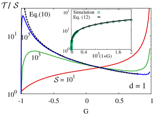
We provide a heuristic argument that predicts both a non-monotonic dependence of lifetime on greediness and a huge maximum for greediness $G\approx-1$ (Fig. 2). Here, starvation proceeds in two stages: (i) The forager first carves a critical desert of length $L_{c}$ by repeatedly reaching either edge of the desert within $\mathcal{S}$ steps after food is consumed. The critical length is defined by a forager of capacity $\mathcal{S}$ typically starving if it attempts to cross a desert of this length. We denote the time to create this critical-length desert as $\mathcal{T}_{c}$. (ii) Once the desert length reaches $L_{c}$, the forager likely starves if it attempts to cross the desert. That is, the far side is unreachable and thus irrelevant. The time for this second stage is just the lifetime of a forager in a semi-infinite desert, $\mathcal{T}_{\rm SI}$.

Figure 2: Dependence of the scaled forager lifetime $\mathcal{T}/\mathcal{S}$ on greediness $G$ in $d=1$ and $d=2$. The inset compares simulations with the analytic result (12) for $G$ close to $-1$ and $\mathcal{S}=10^{6}$. Dotted curves in $d=2$ correspond to a non-backtracking walk (see summary text).

We now estimate the quantities $L_{c}$, $\mathcal{T}_{c}$, and $\mathcal{T}_{\rm SI}$. The time for a forager to reach food when it starts a unit distance from food in a desert of length $k$ is given by $t_{1}(k)=\frac{1-p}{p}\,k+3-\frac{2}{p}$ (see App. A). Therefore the time for the desert to grow to the critical length $L_{c}\gg 1$ is

$$\mathcal{T}_{c}=\sum_{k=1}^{L_{c}}t_{1}(k)\simeq\frac{1-p}{p}\,\frac{L_{c}^{2}}{2}.$$ (1)

We determine $L_{c}$ by equating the typical time to cross a desert of this length, $t_{\times}\simeq\frac{2}{3}L_{c}^{2}+\frac{4L}{3p}$ (see App. A), to $\mathcal{S}$. This gives two behaviors: $L_{c}\simeq\sqrt{3\mathcal{S}/2}$ for $p\gg 1/\sqrt{\mathcal{S}}$, and $L_{c}\simeq 3p\mathcal{S}/4$ for $p\ll 1/\sqrt{\mathcal{S}}$. Thus the time to reach the critical-length desert is

$$\mathcal{T}_{c}\simeq\begin{cases}\displaystyle{3(1\!-\!p)\mathcal{S}/4p}&\qquad p\gg 1/\sqrt{\mathcal{S}}\,,\\[4.26773pt] \displaystyle{9p\mathcal{S}^{2}/32}&\qquad p\ll 1/\sqrt{\mathcal{S}}\,.\end{cases}$$ (2)

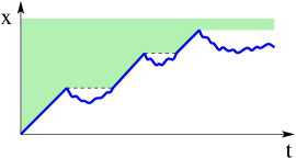
For the semi-infinite geometry, a typical trajectory consists of segments where the forager moves ballistically into the food-containing region, interspersed by diffusive segments in the desert (Fig 3). As long as the diffusive segment lasts less than $\mathcal{S}$ steps, the forager returns to the food/desert interface and a new cycle of consumption and subsequent diffusion begins. A ballistic segment of $m$ consecutive steps towards food (followed by a step away) occurs with probability $p^{m}(1-p)$. The average time $t_{b}$ for this ballistic segment is $t_{b}=\sum_{m\geq 1}m\,p^{m}\,(1\!-\!p)=p/(1\!-\!p)$. The probability $\mathcal{R}$ for a diffusive segment to return to food within $\mathcal{S}$ steps is the integral of the first-passage probability for a forager that starts at $x=1$ to reach $x=0$ within time $\mathcal{S}$ R01 :

$$\mathcal{R}=\int_{0}^{\mathcal{S}}dt\,\,\frac{e^{-1/4Dt}}{\sqrt{4\pi Dt^{3}}}=\mathrm{erfc}(1/\sqrt{4D\mathcal{S}})\,,$$

where erfc$(\cdot)$ is the complementary error function. The average number of returns is $\langle r\rangle=\sum_{r\geq 1}r\,\mathcal{R}^{r}(1\!-\!\mathcal{R})=\mathcal{R}/(1\!-\!\mathcal{R})\simeq\sqrt{\pi\mathcal{S}/2}$ for $\mathcal{S}\to\infty$, where the asymptotics of the error function gives the final result, and we take the diffusion coefficient $D=\frac{1}{2}$. For a forager that does return within $\mathcal{S}$ steps, the return time $t_{r}$ is thus

$$t_{r} =\frac{1}{\mathcal{R}}\int_{0}^{\mathcal{S}}dt\,t\,\frac{1}{\sqrt{4\pi Dt^{3}}}\,\,e^{-1/4Dt}\simeq\sqrt{\frac{2\mathcal{S}}{\pi}}-1\,.$$

Figure 3: Schematic illustration of the space-time trajectory of a greedy forager in the semi-infinite geometry. The shaded region denotes food.

The total trajectory therefore contains $\langle r\rangle=\sqrt{\pi\mathcal{S}/2}$ elements, each of which are comprised of a ballistic and a diffusive segment. The time for each element equals $t_{b}+t_{r}$. There is also the final and fatal diffusive segment of exactly $\mathcal{S}$ steps. Consequently, the forager lifetime $\mathcal{T}_{\rm SI}$ in the semi-infinite geometry is

$$\mathcal{T}_{\rm SI} \simeq\langle r\rangle(t_{b}+t_{r})+\mathcal{S}\simeq\frac{2p-1}{1-p}\,\sqrt{\frac{\pi\mathcal{S}}{2}}+2\mathcal{S}\,.$$ (3)

From (2) and (3), we estimate the forager lifetime as

$$\mathcal{T}\simeq\begin{cases}\displaystyle{\Big{[}\frac{3(1\!-\!p)}{4p}+2\Big{]}\mathcal{S}+\frac{2p\!-\!1}{(1\!-\!p)}\,\sqrt{\frac{\pi\mathcal{S}}{2}}}\,,&p\gg 1/\sqrt{\mathcal{S}}\,,\\[9.95863pt] \displaystyle{\frac{9}{32}\,p\mathcal{S}^{2}+2\mathcal{S}}+\frac{2p\!-\!1}{(1\!-\!p)}\,\sqrt{\frac{\pi\mathcal{S}}{2}}\,,&p\ll 1/\sqrt{\mathcal{S}}\,.\end{cases}$$ (4)

Two important consequences follow (Fig. 2):

• When $\mathcal{S}$ exceeds a critical value, it is easily seen that $\mathcal{T}$ is decreasing with $p$, except for $p\to 0$ and $p\to 1$. Since $\mathcal{T}$ diverges as $p\to 1$, the dependence of lifetime on greediness is non-monotonic!

• For $p\simeq 1/\sqrt{\mathcal{S}}$, Eqs. (4) give a common lifetime $\mathcal{T}\sim\mathcal{S}^{3/2}$—a huge maximum for large $\mathcal{S}$ ! This maximum induces a second non-monotonicity in the negative greed (food averse) regime.

III One-Dimensional Solution

We now outline the analytical solution for the forager lifetime that confirms and quantifies the above heuristic picture. The basic quantity is the probability $V_{k}$ that the forager has eaten $k$ times at the instant of starvation. This quantity can be written as

$$V_{k}=\Big{[}1-\sum_{t=0}^{\mathcal{S}}\,F_{k}(t)\Big{]}\,\,\prod_{j=1}^{k-1}\sum_{t=0}^{\mathcal{S}}\,F_{j}(t)\,.$$ (5)

Here $F_{j}(t)$ is the first-passage probability that a greedy forager that is a unit distance from either edge of a desert of $k$ empty sites first reaches either edge at time $t$. The sum is thus the probability that this forager escapes a desert of $j$ empty sites, and the product is the probability that this forager successively escapes a desert of 1,2,3,…, $k-1$ empty sites. Finally the leading factor is the probability that the forager does not escape a desert of $k$ empty sites.

We may now write the average forager lifetime as

$$\mathcal{T} =\sum_{k\geq 0}\,\big{[}\sum_{j=1}^{k-1}\tau_{j}\big{]}\,V_{k}+\mathcal{S}\,.$$ (6)

Here

$$\tau_{j}=\frac{\sum_{0\leq t\leq\mathcal{S}}\,t\,F_{j}(t)}{\sum_{0\leq t\leq\mathcal{S}}\,F_{j}(t)}$$

is the conditional average time for a greedy forager to successfully escape a desert of $j$ empty sites when it starts one lattice spacing from either edge. The quantity $\sum_{j=1}^{k-1}\tau_{j}$ is the conditional time for the forager to successively escape deserts of 1,2,3,…, $k-1$ empty sites. Consequently, the first term in (6) is that total time that the forager takes to carve a desert of $k$ empty sites and the last factor, $\mathcal{S}$, is the time for the last and fatal excursion in this desert.

To explicitly evaluate the forager lifetime in (6), we need the first-passage probability for a greedy forager, $F_{k}(t)$. This first-passage probability can be related to the unperturbed first-passage probability $f_{k}(t)$ of a symmetric random walk by the convolution

$$F_{k}(t)=p\,\delta_{t,1}+(1-p)\sum_{t^{\prime}\leq t-1}f_{k-2}(t^{\prime})\,F_{k}(t-t^{\prime}-1)\,.$$ (7)

The first term accounts for a forager that reaches food in a single step. The second term accounts for the forager hopping to the interior of the interval. In this case, the walker is at $x=2$ or $k-2$ and hops symmetrically until it again reaches either $x=1$ or $k-1$. Thus the relevant first-passage probability is that for an unbiased random walk that starts at $x=2$ or $k-2$ on $[1,k-1]$. Once the walker first reaches either $x=1$ or $k-1$, the process renews and the subsequent propagation involves $F_{k}$. Since one time unit is used in the first hop to the right, the walker must reach the boundary in the remaining time $t-t^{\prime}-1$ steps. We solve Eq. (7) by substituting in the generating functions

$${\widetilde{f}_{k}}(z)=\sum_{t\geq 1}f_{k}(t)\,z^{t}\,,\qquad{\widetilde{F}_{k}}(z)=\sum_{t\geq 1}F_{k}(t)\,z^{t}\,.$$

The generating functions reduce the convolution in Eq. (7) to an algebraic relation that is readily solved to give

$${\widetilde{F}_{k}}(z)=\frac{pz}{1-(1-p)\,z\,{\widetilde{f}_{k-2}}(z)}\,.$$ (8)

The next step is to substitute the well-known result for the Laplace transform of the first-passage probability R01

$${\widetilde{f}_{k}}(s) =\text{sech}\sqrt{\frac{s}{D}}\,k\left[\sinh\Big{(}\sqrt{\frac{s}{D}}\Big{)}+\sinh\Big{(}\sqrt{\frac{s}{D}}(k\!-\!1)\Big{)}\right]\,,$$

$$\underset{s\to 0}{\longrightarrow}1-\sqrt{\frac{s}{D}}\tanh\sqrt{\frac{sk^{2}}{4D}}k+\cdots\,.$$

into Eq. (8). We also convert the discrete generating function to a continuous Laplace transform by replacing $z\to 1-s$. This construction is asymptotically exact in the limit $z\to 1$ or $s\to 0$, which corresponds to the long-time limit in the time domain. Following these steps, the Laplace transform of the first-passage probability for the greedy forager for $s\to 0$ and $k\to\infty$ is

$${\widetilde{F}_{k}}(s)=\bigg{(}1+\frac{1-p}{p}\sqrt{\frac{s}{D}}\tanh\sqrt{\frac{sk^{2}}{4D}}\bigg{)}^{-1}.$$ (9)

Using the above first-passage probability for a greedy forager in a finite desert, and also making use of standard Laplace transform manipulations, we can determine both $\tau_{k}$ and $V_{k}$ in terms of ${\widetilde{F}_{k}}(s)$. When these quantities are expressed in terms of ${\widetilde{F}_{k}}(s)$ in Eq. (6), we can finally determine the forager lifetime $\mathcal{T}$. These steps are somewhat tedious and all the details are given in Ref. BRB17 .

There are two limiting cases where the forager lifetime has very different asymptotic behaviors: $p\gg 1/\sqrt{\mathcal{S}}$ and $p\ll 1/\sqrt{\mathcal{S}}$. In the former case, we find

$$\mathcal{T} \simeq\mathcal{S}\,\frac{1\!-\!p}{p}\int_{0}^{\infty}\!\!\!d\theta\,V_{\theta}\int_{0}^{\theta}\!\!\frac{du}{u}\sum_{j\geq 0}\frac{4}{v^{2}}\left\{1\!-\!e^{-v^{2}}\!\left[1\!+\!v^{2}\right]\right\}+\mathcal{S}\,.$$ (10)

Here $v=(2j\!+\!1)/u$, $\theta=n/(\pi\sqrt{D\mathcal{S}})$, with $n$ the number of sites visited by the forager at starvation. Additionally,

$$V_{\theta} \simeq\frac{4(1\!-\!p)}{p\theta}\sum_{j\geq 0}e^{-w^{2}-Q}\,,\quad Q=\frac{2(1-p)}{p}\sum_{j\geq 0}E_{1}(w^{2})\,,$$

where $w=(2j\!+\!1)/\theta$, and $E_{1}(x)=\int_{1}^{\infty}\frac{dt}{t}\,e^{-xt}$ is the exponential integral. Because the function $V_{\theta}$ depends on $p$, the greedy forager lifetime $\mathcal{T}$ does not merely equal $\mathcal{T}$ for the non-greedy forager times $\frac{1-p}{p}$. Our result (10) agrees with numerical simulations for large $\mathcal{S}$ (Fig. 2).

Deep in the negative greed regime $p\ll 1/\sqrt{\mathcal{S}}$, Eq. (9) simplifies to

$${\widetilde{F}}_{k}(s)\simeq\left(1+\frac{k}{2pD}s\right)^{-1}\,.$$ (11)

Following the same steps as given above now leads to

$$\mathcal{T}=\sum_{k\geq 1}\frac{k^{2}}{2p\mathcal{S}}\,e^{-{2pD\mathcal{S}}/{k}}\exp\left[-\int_{1}^{k}e^{-{2pD\mathcal{S}}/{x}}\,dx\right]+\mathcal{S}\,,$$ (12)

whose numerical evaluation matches the simulation results in the regime $p\ll 1/\sqrt{\mathcal{S}}$ (Fig. 2 inset).

IV Two Dimensions

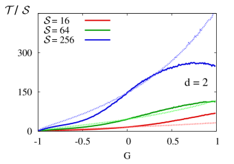
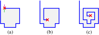
Surprisingly, simulations show that the forager lifetime again varies non-monotonically with (positive) greed, but in the opposite sense compared to one dimension (Fig. 2). A perfectly greedy forager has a smaller lifetime than one that is not quite as avaricious. We can explain this feature in a simple way: Because a random walk is recurrent in two dimensions, it will certain form closed loops along its trajectory F68 ; W94 . Suppose that a perfectly greedy forager is about to form such a closed loop (Fig. 4(a)). At this point, the forager has only two possible choices for the next step. One of them leads outside the incipient closed loop and the other leads inside. If the latter choice is made, a “moat” is created by the previous trajectory.

Figure 4: A random-walk trajectory that leads to trapping of a perfectly greedy forager. (a) Forager ($\times$) at the decision point. (b) Forager hops to the interior region (shaded). (c) Food in the interior is completely consumed, so that the forager ($\times$) may be trapped inside the newly created desert.

Once inside the moat, a perfectly greedy forager always consumes food in its nearest neighborhood. Ultimately, this interior food is mostly or completely depleted (the latter is shown in Fig. 4(c)). While the former case is more likely, the remaining food will be scarce and isolated. Thus the forager creates and then becomes trapped inside a (perhaps slightly imperfect) desert.

Conversely, if the greediness $G<1$, a forager that encounters the moat from the interior can cross it with a non-zero probability and thereby reach food on the outside. This mechanism provides a route for the forager to escape the desert and survive longer than if it remained strictly inside. This argument indicates that the forager lifetime should be a decreasing function of $G$ as $G\to 1$, as confirmed by simulations (Fig. 2). Also in stark contrast to one dimension, there is no peak in the forager lifetime for negative greed, at least for the values of $\mathcal{S}$ that we were able to simulate.

V Summary

Greed plays a paradoxical role in the lifetime of a greedy random-walking forager, which moves preferentially towards local food for positive greediness, and away from food for negative greediness. The lifetime depends non-monotonically on greediness when the forager capacity is sufficiently large. Moreover, the sense of the non-monotonicity is opposite in one and two dimensions. In $d=1$, the forager lifetime exhibits a huge peak of the order of $S^{3/2}$ for $G\approx-1$, scales as $\mathcal{S}^{1/2}/(1-G)$ for $G\to 1$, while $\mathcal{T}\simeq\mathcal{S}$ throughout the rest of the range of $G$. Determining these intriguing properties rests on solving a challenging non-Markovian first-passage problem in which the forager motion is locally biased when food is in the forager’s nearest neighborhood.

A variety of questions remain open. Can one make analytical progress in two dimensions? What is the behavior of the lifetime in greater than two dimensions? Simulations are not useful here because the lifetime is extremely long for non-negligible greed and memory/computation time constraints become prohibitive. On a biological note, greed can be viewed as endowing a forager with a minimal information processing capability. A related mechanism is for the forager to perform a non-backtracking random walk (previous step is not retraced). The forager lifetime increases monotonically with the probability of not backtracking (Fig. 2; here $1-G$ is a proxy for the backtracking probability) and perfect non-backtracking is superior to perfect greed. It would be useful to understand how to most effectively increase the forager lifetime with minimal information-processing enhancements to random-walk motion.

We acknowledge support from the European Research Council starting grant FPTOpt-277998 (OB), from grants DMR-1608211 and DMR-1623243 from the National Science Foundation (UB and SR), by the John Templeton Foundation (SR), and from grant 2012145 from the U.S.-Israel Binational Science Foundation (UB).

Appendix A Escape From An Interval

We determine the first-passage properties of a random walk in a finite interval of length $L$ whose hopping rules are the same as that of a greedy forager. That is, a walk in the interior hops equiprobably to the left and right, while a walk at either $x=1$ or $x=L-1$ hops to the edge of the interval with probability $p$ and into the interior with probability $1-p$ (Fig. 5). For these hopping rules, we calculate the exit probabilities to each side of the interval, the unconditional time to exit either side of the interval, and the conditional exit time to exit by each edge of the interval. We will use the result for the unconditional exit time to derive Eq. (1), from which we will heuristically argue that the lifetime of a forager with a sufficiently large capacity varies non-monotonically with greediness.

Figure 5: Hopping probabilities for a greedy forager inside a desert of length $L$.

Let $E_{n}$ be the probability that the forager, which starts at site $n$, exits the interval via the left edge. The exit probabilities satisfy the backward equations

$$\begin{split}&E_{1}=p+qE_{2}\,,\\ &E_{n}=\tfrac{1}{2}E_{n-1}+\tfrac{1}{2}E_{n+1}\qquad 2\leq n\leq L-2\,,\\ &E_{L-1}=qE_{L-2}\,.\end{split}$$ (13)

No boundary conditions are needed, as the distinct equations for $n=1$ and $n=L-1$ fully determine the exit probabilities. As we shall see, $E_{n}=0$ not at $n=L$, but at different value of $n$, and similarly for the point where $E_{n}=1$.

Since the deviation to random-walk motion occurs only at the boundaries, we attempt a solution that has the random-walk form in the interior of the interval: $E_{n}=A+Bn$. This ansatz automatically solves the interior equations ($2\leq n\leq L-2$), while the boundary equations for $n=1$ and $n=L-1$ give

$$E_{1}=p+qE_{2} ~{}\longrightarrow~{}A+B=p+q(A+2B)\,,$$

$$E_{L-1}=qE_{L-2} ~{}\longrightarrow~{}A+B(L-1)=q\big{(}A+B(L-2)\big{)}\,,$$

from which $A$ and $B$ are

$$A=\frac{p(L-2)+1}{pL+2(1-2p)}\,,\qquad B=-\frac{p}{pL+2(1-2p)}\,.$$

Thus the probability that a greedy random walk that starts at $x=n$ exits via the left edge of the interval is

$$E_{n}=A+Bn=\frac{L-n+\frac{1}{p}(1-2p)}{L+\frac{2}{p}(1-2p)}\,,$$ (14)

while the exit probability via the right edge is $1-E_{n}$. As might be expected for a perturbation that applies only at the boundary, the overall effect of greed on the exit probability is small: the exit probability changes from $E_{n}=1-\frac{n}{L}$ for $p=\frac{1}{2}$ to $E_{n}=1-\frac{n-1}{L-2}$ for $p=1$. That is, the effective interval length changes from $L$ to $L-2$ as $p$ increases from $\frac{1}{2}$ to 1.

Similarly, let $t_{n}$ be the average time for a greedy random walker to reach either edge of the interval when the walk starts at site $n$. These exit times satisfy the backward equations

$$\begin{split}&t_{1}=p+q(t_{2}+1)\,,\\ &t_{n}=\tfrac{1}{2}t_{n-1}+\tfrac{1}{2}t_{n+1}+1\qquad 2\leq n\leq L-2\,,\\ &t_{L-1}=p+q(t_{L-2}+1)\,.\end{split}$$ (15)

Again, no boundary conditions are needed, as the equations for $n=1$ and $n=L-1$ are sufficient to solve (LABEL:tn). We attempt a solution for these second-order equations that has the same form as in the case of no greed: $t_{n}=a+bn+cn^{2}$. Substituting this ansatz into (LABEL:tn) immediately gives $c=-1$, while the equations for $t_{1}$ and $t_{L-1}$ lead to the conditions

$$-1+a+b=q(-4+a+2b)+1\,,$$

$$-(L-1)^{2}+b(L-1)+a$$

$$\qquad\qquad~{}~{}~{}=q\big{[}-(L-2)^{2}+b(L-2)+a\big{]}+1\,.$$

Solving these equations, the average exit time to either edge of the interval when starting from site $n$ is

$$t_{n}=n(L-n)-\frac{2p-1}{p}(L-2)\,.$$ (16)

This gives a parabolic dependence of $t_{n}$ on $n$ that is shifted slightly downward compared to the case of no greed, as $p$ ranges from $\frac{1}{2}$ to 1. Notice again that $t_{n}=0$ not at $n=0$ and $n=L$, but rather at points between $n=0$ and 1 and between $n=L-1$ and $L$ for $p>\frac{1}{2}$. This overall shift leads to a tiny change in each $t_{n}$, except when the forager starts one site away from the boundary.

Finally, we determine the conditional exit times, $t^{\pm}_{n}$, defined as the time to reach left edge of the interval when starting from site $n$ (for $t^{-}$) and to the right edge (for $t^{+}$), conditioned on the walker exiting only by the specified edge. We focus on $t^{-}_{n}$, because once $t^{-}_{n}$ is determined, we can obtain $t^{+}_{n}$ via $t^{+}_{n}=t^{-}_{L-n}$. The conditional exit times $t^{-}_{n}$ satisfy

$$\begin{split}&u_{1}=qu_{2}+E_{1}\,,\\ &u_{n}=\tfrac{1}{2}u_{n-1}+\tfrac{1}{2}u_{n+1}+E_{n}\qquad 2\leq n\leq L-2\,,\\ &u_{L-1}=qu_{L-2}+E_{L-1}\,,\end{split}$$ (17)

where $u_{n}\equiv E_{n}t^{-}_{n}$, with $E_{n}$, the exit probability to the left edge, given by Eq. (14). Because Eqs. (LABEL:un) are second-order with an inhomogeneous term that is linear in $n$, the general solution is a cubic polynomial: $u_{n}=a+bn+cn^{2}+dn^{3}$. Substituting this form into Eq. (LABEL:un) for $2\leq n\leq L-2$, we obtain the conditions $c=-A$ and $d=-B/3$, where $A$ and $B$ are the coefficient of $E_{n}$ in Eq. (14). The remaining two coefficients are determined by solving the equations for $u_{1}$ and $u_{L-1}$ and the final results for the coefficients $a,b,c,d$ in $u_{n}$ are:

$$a =\frac{2(L\!-\!2)(1\!-\!2p)\big{[}p^{2}(L\!-\!4)(L+\frac{3}{p}(1\!-\!p))+3\big{]}}{3p^{3}\big{[}L+\frac{2}{p}(1-2p)\big{]}^{2}}\,,$$

$$b =\frac{2p^{2}\big{[}L(L^{2}\!-\!6L\!+\!6)\!+\!8\big{]}+6pL(L\!-\!3)\!+\!6L\!-\!8p}{3p^{2}\big{[}L+\frac{2}{p}(1-2p)\big{]}^{2}}\,,$$

$$c =-\frac{L+\frac{1}{p}(1-2p)}{L+\frac{2}{p}(1-2p)}\,,$$

$$d =-\frac{1}{3}\,\frac{1}{L+\frac{2}{p}(1-2p)}\,.$$ (18)

Finally, the conditional exit time to the left edge is $t_{n}^{-}=u_{n}/E_{n}$, with $u_{n}=a+bn+cn^{2}+dn^{3}$, and $E_{n}$ already determined in Eq. (14). We are particularly interested in $t^{-}_{L-1}$, the conditional time for a walk that starts at $x=L-1$ to reach $x=0$. From Eqs. (14) and (A), the limiting behavior of this crossing time for large $L$ is

$$t^{-}_{L-1}\equiv t_{\times}\simeq\frac{2}{3}\,L^{2}+\frac{4}{3}\,\frac{L}{p}\,,$$ (19)

References

- (1) E. L. Charnov, Theor. Popul. Biol. 9, 129 (1976).
- (2) P. Knoppien and J. Reddingius, J. Theor. Biol. 114, 273 (1985).
- (3) D. W. Stephens and J. R. Krebs, Foraging Theory, (Princeton University Press, Princeton, NJ, 1986).
- (4) W. J. O’Brien, H. I. Browman, and B. I. Evans, Am. Sci. 78, 152 (1990).
- (5) J. W. Bell, Searching Behaviour, the Behavioural Ecology of Finding Resources, Animal Behaviour Series (Chapman and Hall, London, 1991).
- (6) J. P. Anderson, D. W. Stephens, and S. R. Dunbar, Behav. Ecol. 8, 307 (1997).
- (7) L. D. Kramer and R. L. McLaughlin, Am. Zool. 41, 137 (2001).
- (8) J. G. March, Organ. Sci. 2, 71 (1991).
- (9) T. Gueudré, A. Dobrinevski, J.-P. Bouchaud, Phys. Rev. Lett. 112, 050602 (2014).
- (10) H. Robbins, Bull. Am. Math. Soc. 58 527 (1952).
- (11) J. C. Gittins, J. Roy. Statist. Soc. Ser. B (Methodological), 41, 148 (1979).
- (12) T. S. Ferguson, Statist. Sci. 4, 282 (1989).
- (13) http://www.feynmanlectures.info/other/Feynmans_Restaurant_Problem_Revealed.html.
- (14) T. T. Hills, M. N. Jone, and P. M. Todd, Psychol. Rev. 119 431 (2012).
- (15) J. T. Abbott, J. L. Austerweil, and T. L. Griffiths, Psychol. Rev. 122 558 (2015).
- (16) G. Viswanathan, S. V. Buldyrev, S. Havlin, M. Da Luz, E. Raposo, and H. E. Stanley, Nature 401, 911 (1999).
- (17) O. Bénichou, M. Coppey, M. Moreau, P.-H. Suet, and R. Voituriez, Phys. Rev. Lett. 94, 198101 (2005).
- (18) G. Oshanin, H. Wio, K. Lindenberg, and S. Burlatsky, J. Phys. Condens. Matter 19, 065142 (2007).
- (19) M. A. Lomholt, K. Tal, R. Metzler, and K. Joseph, Proc. Natl. Acad. Sci. (USA) 105, 11055 (2008).
- (20) P. C. Bressloff and J. M. Newby, Phys. Rev. E 83, 061139 (2011).
- (21) G. M. Viswanathan, M. G. E. da Luz, E. P. Raposo, and H. E. Stanley, The Physics of Foraging, (Cambridge University Press, Cambridge, 2011).
- (22) V. V. Palyulin, A. V. Chechkin, and R. Metzler, Proc. Natl. Acad. Sci. (USA) 111, 2931 (2014).
- (23) V. Tejedor, R. Voituriez, and O. Bénichou, Phys. Rev. Lett. 108, 088103 (2012).
- (24) O. Bénichou and S. Redner, Phys. Rev. Lett. 113, 238101 (2014).
- (25) M. Chupeau, O. Bénichou, and S. Redner, J. Phys. A: Math. & Theor. 49, 394003 (2016).
- (26) T. H. Cormen, C. E¿ Leiserson, R. L. Rivest, and C. Stein, Introduction to Algorithms, ed., (MIT Press, Cambridge, MA 2009).
- (27) J. Bang-Jensen, G. Gutin and A. Yeo, Discrete Optimization 1, 121 (2004).
- (28) C. Moore and S. Mertens, The Nature of Computation, (Oxford University Press, Oxford, UK, 2011).
- (29) J. B. Kruskal, Proc. Am. Math. Soc. 7, 48 (1956).
- (30) C. M. Newman and D. L. Stein, Phys. Rev. Lett. 72, 2286 (1994).
- (31) https://en.wikipedia.org/wiki/Greedy_algorithm.
- (32) H. C. Berg and D. A. Brown, Nature 239, 500 (1972).
- (33) H. C. Berg and E. M. Purcell, Biophys. J. 20, 193 (1977).
- (34) P. N. Devreotes and S. H. Zigmond, Annu. Rev. Cell Biol. 4, 649 (1988).
- (35) E. M. Buchkremer and K. Reinhold, Behav. Ecol. 19, 984 (2008).
- (36) M. Otte, N. Correll, and E. Frazzoli, in IEEE International Conference on Intelligent Robots and Systems (IROS), Tokyo, Japan, 2013.
- (37) Artificial Life IX: Proceedings of the Ninth International Conference on the Simulation and Synthesis of Living Systems, J. Pollack, M. A. Bedau, P. Husbands, R. A. Watson, and T. Ikegami eds. (MIT Press, Cambridge, MA 2004).
- (38) See U. Bhat, S. Redner, and O. Bénichou, arXiv.org:1704.05861, for all calculational details.
- (39) S. Redner, A Guide to First-Passage Processes, (Cambridge University Press, Cambridge, UK, 2001).
- (40) W. Feller, Introduction to Probability Theory and its Applications, ed., (J. Wiley & Sons, New York, 1968)
- (41) G. H. Weiss, Aspects and Application of the Random Walk, (North-Holland, Amsterdam, 1994).