CMU DeepLens: Deep Learning For Automatic Image-based Galaxy-Galaxy Strong Lens Finding
Abstract
Galaxy-scale strong gravitational lensing is not only a valuable probe of the dark matter distribution of massive galaxies, but can also provide valuable cosmological constraints, either by studying the population of strong lenses or by measuring time delays in lensed quasars. Due to the rarity of galaxy-scale strongly lensed systems, fast and reliable automated lens finding methods will be essential in the era of large surveys such as LSST, Euclid, and WFIRST. To tackle this challenge, we introduce CMU DeepLens, a new fully automated galaxy-galaxy lens finding method based on Deep Learning. This supervised machine learning approach does not require any tuning after the training step which only requires realistic image simulations of strongly lensed systems. We train and validate our model on a set of 20,000 LSST-like mock observations including a range of lensed systems of various sizes and signal-to-noise ratios (S/N). We find on our simulated data set that for a rejection rate of non-lenses of 99%, a completeness of 90% can be achieved for lenses with Einstein radii larger than 1.4″ and S/N larger than 20 on individual -band LSST exposures. Finally, we emphasize the importance of realistically complex simulations for training such machine learning methods by demonstrating that the performance of models of significantly different complexities cannot be distinguished on simpler simulations. We make our code publicly available at https://github.com/McWilliamsCenter/CMUDeepLens.
keywords:
gravitational lensing: strong – methods: statistical.1 Introduction
Strong gravitational lensing, the serendipitous appearance of multiple images or extended arcs due to distant quasars or galaxies almost directly behind a massive object along the same line-of-sight, finds many important applications both astrophysical and cosmological. It is in particular a well-established probe of overall gravitational potential of massive galaxies. For example, moderate-sized samples of galaxy-scale strong lenses from the Sloan Lens ACS (SLACS) survey (Bolton et al., 2006) have been used to derive ensemble constraints on the total matter profile in massive elliptical galaxies (e.g. Koopmans et al., 2006; Auger et al., 2010; Barnabè et al., 2011). As a cosmological probe, time delays in multiply imaged strongly lensed quasars can be used to derive independent constraints on the Hubble constant (e.g. Refsdal, 1964; Suyu et al., 2010; Bonvin et al., 2017), but even without time delays strongly lensed systems can constrain cosmological parameters and in particular the dark energy equation of state (e.g. Collett & Auger, 2014; Cao et al., 2015). See, e.g., Treu (2010) for a review of results using strong lensing by galaxies.
Upcoming large sky surveys such as the Large Synoptic Survey Telescope (LSST111https://www.lsst.org/lsst/; LSST Science Collaboration et al. 2009), Euclid222http://sci.esa.int/euclid/, http://www.euclid-ec.org (Laureijs et al., 2011), and the Wide-Field Infrared Survey Telescope (WFIRST333https://wfirst.gsfc.nasa.gov/; Spergel et al. 2015) will produce datasets that include unprecedented numbers of galaxy-scale strong lenses. For example, Collett (2015) predicts galaxy-scale strong lens systems in LSST and Euclid. This lens population is expected to be dominated by intermediate-redshift (–1) elliptical galaxies, with blue source galaxies. Clearly, the challenge will be to detect those galaxy-scale strong lenses efficiently and in a way that results in an easily-quantifiable selection function for further scientific investigation. LSST and Euclid present different challenges for automated galaxy-scale strong lens detection. The LSST imaging will have 6 photometric bands, enabling us to distinguish between objects with different colors, but at low resolution compared to space-based imaging. In contrast, the Euclid imaging will be far higher resolution but with only a single optical passband. Thus, neither survey achieves the optimal setup for galaxy-scale strong lens detection, i.e., high-resolution multi-color imaging. The space-based, multi-band near-infrared data from WFIRST in principle provides a dataset that is closer to optimal, though the galaxy populations probed may differ due to the fact that the imaging is at near-infrared wavelengths.
Most automated image-based lens finding methods proposed so far have been based on the detection of arc and ring structures in the images. The ARCFINDER method (Alard, 2006; More et al., 2012) relies for instance on a local elongation estimator, at the pixel level. Other approaches to arc finding purely based on morphology include those described by Seidel & Bartelmann (2007); Kubo & Dell’Antonio (2008); Bom et al. (2017). When considering specifically galaxy-scale strong lenses, arcs can often be obscured by the light of the lens galaxy. Several methods have been proposed to perform a first subtraction step of the lens galaxy to facilitate the detection of faint arcs. The RingFinder algorithm proposed in Gavazzi et al. (2014) uses a multi-band differencing scheme to reveal faint blue arcs surrounding early type galaxies. Joseph et al. (2014) proposed an alternative subtraction scheme, which does not require multi-band images, based on a PCA decomposition of the lens light profile. A different approach based on physical lens modeling was initially proposed in Marshall et al. (2009) for high resolution space-based images and revisited in Brault & Gavazzi (2015) for ground-based images. In this class of methods, a simple model including a background source and a foreground deflector is fitted on each lens candidate, and a classification as a possible lens is made based on the predicted model parameters.
As an example of automated lens searches, some of these methods were applied to the Strong Lensing Legacy Survey (SL2S; Cabanac et al., 2007), a survey from the Canada-France-Hawaii Telescope Legacy Survey (CFHTLS) covering an approximate area of 150 deg2. The ARCFINDER was applied to the survey in More et al. (2012), producing a final sample of 127 potential lenses, mostly on group and cluster mass scales. The authors report that the algorithm produced an average of 1,000 candidates per deg2 requiring a significant amount of further visual inspection. The RingFinder algorithm was also applied to the CFHTLS data (Gavazzi et al., 2014) but concentrated on galaxy-scale lenses by pre-selecting early-type galaxies. This algorithm produced on average a more manageable 18 candidates per deg2, and a final sample of 330 high probability lenses after visual inspection. In this particular case, the authors reported that visual inspection required an estimated 30 person-minutes per deg2. At this rate, next generation surveys such as Euclid (15000 deg2) or LSST (20000 deg2) would still require a very significant investment of human time.
One approach to scale the visual inspection effort to the size of these surveys is to use crowdsourcing. This is the idea behind the Space Warps project (Marshall et al., 2015; More et al., 2015), which crowdsourced the visual inspection of a sample of 430,000 images from the CHFTLS to a crowd of 37,000 citizen scientists, yielding a new sample of gravitational lens candidates. 59 of these candidates were previously missed by robotic searches, while 20 known lenses were missed by the volunteers. These results show a complementarity between the two approaches, and crowdsourced visual inspection could prove very valuable in screening lens candidates found by automated searches. The authors further estimate that a similar crowdsourcing effort can be scaled up to LSST sizes, where a considerable crowd of volunteers could visually inspect LSST targets in a matter of weeks.
The image classification problem involved in strong lens finding is a notoriously challenging task that has received considerable attention in the broader field of computer vision and machine learning. Very recently, a new class of models based on the Deep Learning framework (LeCun et al., 2015) has been able to surpass human accuracy in similar image classification tasks (He et al., 2015a). Such models are therefore extremely promising for gravitational lens searches as they could prove more reliable than non-expert human inspection and therefore dramatically reduce the amount of human time investment for future surveys. Some Deep Learning models have already been proposed in an astrophysical context, most notably for automatic identification of galaxy morphologies (Dieleman et al., 2015), performing star-galaxy classification (Kim & Brunner, 2017), estimating photometric redshifts (Hoyle, 2016), or for generative models of galaxy images (Ravanbakhsh et al., 2016).
The idea of using Deep Learning for detecting strongly lensed systems has recently been explored by several groups. For instance, Petrillo et al. (2017) recently published an application on the Kilo Degree Survey (KiDS; de Jong et al., 2015). This method, as well as all other Deep Learning methods currently under investigation for this task are based on deep Convolutional Neural Networks (CNNs; Lecun et al., 1998; Krizhevsky et al., 2012), a powerful architecture for image detection and classification tasks.
In this paper, we present a new approach to strong lens finding, based on deep Residual Networks (He et al., 2015a), an advanced variation of CNNs that constitutes the current state of the art in image classification. As a result, our proposed architecture, named CMU DeepLens, or DeepLens in short, has recently been found to outperform most CNN-based lens finders in a recent blind challenge organised by the Euclid strong lensing working group444http://metcalf1.bo.astro.it/blf-portal/gg_challenge.html (Metcalf et al. 2017, in prep.).
Contrary to most previous methods, such a supervised machine learning approach does not make any prior assumptions on specific features or physical models and instead lets the machine learn from the provided training data which features are the most relevant to the detection of strong lenses. In addition to characterising the performance of our baseline architecture using simulations of lens systems in LSST, we also explore the impact of model and simulation complexity on machine learning-based lens finders.
This paper is structured as follows. In section 2, we provide some background on the Deep Learning framework and introduce the building blocks used in our classifier. In section 3, we detail the DeepLens architecture itself as well as the training procedure. We then describe in section 4 the strong lensing simulation pipeline that was used to generate a set of training and validation images. These simulations are used in section 5 to quantify the performance of our model. Finally, section 6 discusses current limitations as well as several avenues for further improvement of our results, with conclusions provided in section 7.
2 Deep Learning Background
In this first section, we provide a brief overview of the Deep Learning framework and introduce the specific components used in our model.
2.1 The Deep Learning Revolution
Artificial Neural Networks (ANNs) have been an established tool for classification and regression tasks for several decades. In fully connected feedforward models such as the Multilayer Perceptron (MLP), each layer is composed of elementary units (the neurons) performing a simple weighted linear combination over the outputs of all units in the previous layer, followed by the application of a non-linear transform, also known as the activation function. This architecture is illustrated in Figure 1. Let denote the neural layer in a deep architecture, and let denote the number of outputs of layer . Using tensor notations, the output of a given layer of the network can be expressed in terms of the output of the previous layer according to:
| (1) |
where is the element-wise activation function, such as the sigmoid-shaped logistic function , is a dense weight matrix, and is a vector of additive biases applied before the activation function. Here the input is identified by and output is the final layer.
Such a model is trained to perform a specific task by optimising its parameters as to minimise a given loss function. This optimisation is performed by a Stochastic Gradient Descent (SGD) algorithm which iteratively updates the model weights by taking small gradient steps computed over a randomly selected sub-sample of the training set. The computation of these gradients are made tractable in practice using the backpropagation algorithm (Rumelhart et al., 1986), which simply applies the chain rule to efficiently obtain the derivative of the the loss function with respect to the model parameters. This, relies on the idea that the gradients at layer can efficiently be computed by using the gradients at layer . A crucial point of this training procedure is that the gradients of the model are computed starting from the last hidden layer and then propagated through the network back to the first layer .
If trained well, the performance of such a feedforward neural network is expected to increase with the depth of the model, as additional layers allow for a more complex mapping from the input to the output. Even using one hidden layer, a feedforward network –with sufficient number of hidden units– is known to be a universal approximator (Hornik et al., 1989) – that is it can approximate any function to arbitrary precision.
However, until very recently, deep networks with many hidden layers had remained completely unpractical as they were notoriously difficult to train. The main reason is the so-called vanishing gradient effect where the gradient of the cost function decreases exponentially due to the repeated chain rules and eventually vanishes as it is backpropagated through the layers during training. As a result, parameters in lower-level layers could not be tuned well in practice, thus greatly limiting the depth of typical models to a few hidden layers.
While this limitation had remained unsolved for several decades, the Deep Learning revolution was brought about by a conjunction of factors: the emergence of effective procedures to train deep architectures, the explosion of the volume of available training data, and the increase in computing power through Graphical Processing Units (GPU). Amongst the innovations that allowed for deeper models, the ReLU (for rectified linear unit) activation function was introduced in Nair & Hinton (2010). This simple function, defined as , does not saturate contrary to conventional sigmoid functions, leading to much stronger gradients which can be propagated deeper in the models during training. The availability of much larger training sets as well as new regularisation techniques (e.g. dropout regularisation; Hinton et al. 2012; Srivastava et al. 2014) have further made it possible to train large networks without over-fitting. Finally, efficient implementations of neural network architectures on GPUs has accelerated the training process by several orders of magnitudes, compared to CPU implementations. Combining these factors and innovations with the pre-existing Convolutional Neural Network architecture (Lecun et al., 1998, see the next section for details) deep neural networks have suddenly been able to reach significant depth and achieve state-of-the-art results in image classification problems (Krizhevsky et al., 2012).
Deep architectures now achieve state-of-the-art (and some times superhuman) performance in a wide range of applications in computer vision, natural language processing, bioinformatics, data-mining and computer games. We refer interested readers to Goodfellow et al. (2016) for a general introduction.
2.2 Convolutional Neural Networks
Taking into account the specific topological structure and properties of natural images, Lecun et al. (1998) introduced the Convolutional Neural Network (CNN) as an efficient alternative to fully connected architectures for image processing. The building block of CNNs is the convolutional layer which outputs a set of feature maps by convolving an input image with learned local filters. This process is illustrated in Figure 2 where an input RGB image is convolved with a set of eight 3x3 filters to yield eight output feature maps.
More formally, let us consider the input of convolution layer . Considering square images for simplicity, we will denote the height and width in pixels of by , while its depth (i.e. the number of bands or feature maps) will be denoted by , so that . In a similar fashion, we will note the output of convolution layer . In the case of the illustration of Figure 2, while for the input RGB image and for the output feature-maps. With these notations, a single output feature-map of for is expressed as:
| (2) |
where is referred to as the convolution kernel, and it contains a different filter of size for each combination of input and output channels. As in the fully-connected architecture, is a bias parameter (i.e., one scalar parameter per output channel) and is a nonlinearity.
The size of the convolution kernel is generally limited to a few pixels (e.g., ). To capture larger scale information, CNNs follow a hierarchical multi-scale approach by interleaving convolution layers with so-called pooling layers, which apply a downsampling operation to the feature maps. A CNN architecture is a stack of convolution layers and pooling layers, converting the input image into an increasing number of feature maps of progressively coarser resolution. The final feature maps can capture information on the scale of the input image and can reach a high-level of abstraction. Combined with efficient GPU implementations, CNNs have become a standard model for image detection and classification tasks.
2.3 Deep Residual Networks
As mentioned in the previous section, the performance of a deep network generally increases with the number of layers, up to the point at which the model becomes too difficult to train and performances start to degrade. This general rule still applies to CNN architectures, which despite reaching greater depths than previous models have been limited to around a dozen layers. To overcome this well-known difficulty, machine learning research has recently been focused on developing alternative architectures beyond simple CNNs, in an attempt to build deeper models that can still be efficiently trained.
Several very recent developments have lead to significant improvements in model accuracy for classification and detection tasks. For instance, the Inception architecture (Szegedy et al., 2015) allowed the GoogLeNet model to reach a depth of 22 layers, and as a result to win the ImageNet Large-Scale Visual Recognition Challenge 2014 (ILSVRC2014), one of the benchmarks in image classification and object detection. Even more recently, He et al. (2015a) introduced the deep residual learning framework, which allowed the authors to increase the depth of their convolutional model by one order of magnitude to 152 layers while still improving detection and classification accuracy and ultimately winning the ILSVRC2015. These results were even further improved in a follow-up work (He et al., 2016) where the authors successfully trained models as deep as 1000 layers while still improving classification accuracy. The model proposed in our work is directly based on this state-of-the-art deep residual network, or resnet, architecture.
Residual learning aims to tackle the problem of vanishing gradients and difficult optimisation of deep networks by introducing so-called shortcut connections between the input and output of a stack of a few convolution layers, so that instead of learning how to map the input to the output, the convolution layers are only learning their difference, hence the term residual learning. In other words, instead of learning directly a given non linear mapping between input and outputs, residual networks are trained to learn the residual mapping with respect to the identity: . An illustration of a simple residual unit proposed in He et al. (2016) is provided on 3(a), where the left branch corresponds to the shortcut connection and the right branch is learning the residual mapping with a few convolution layers. Deep residual networks are then built by stacking a large number of these residual units.
While this residual learning architecture may seem like a trivial recasting of the mappings in the network, it has been found in practice to be much easier to train in deep networks (He et al., 2015a), for several reasons. First and foremost, this architecture nearly eliminates the vanishing gradients problem by providing an unhindered route for the gradients to backpropagate through the layers using the shortcut connection. Another major advantage is that weight initialisation can be made more robust, given that the weights in a residual connection should be close to zero. Finally, the residual mappings are expected to be simpler than the full mappings, leading to an easier overall optimisation problem.
In this work, we will adopt a specific type of units advocated by He et al. (2016), the pre-activated bottleneck residual unit. Pre-activation refers to the inversion of the conventional ordering of convolution and activation functions. In a classical CNN architecture, the activation function is applied to the output of the convolution, as described in Equation 2, but in a pre-activated architecture, the element-wise activation function is first applied to the input image, followed by the convolution. This alternative architecture is empirically found to yield better performances. These units are built around a stack of 1x1, 3x3, and 1x1 convolution layers (hence the ‘bottleneck’ appellation). This is also empirically found to yield similar performance as a stack of two 3x3 convolutions but for a reduced number of parameters. Figure 3 illustrates two variants of these residual units; 3(a) preserves the dimensions and depth of the input, while 3(b) allows for a downsampling in resolution and an increase in depth by inserting a convolution layer in the shortcut branch. This downsampling of a factor 2 is performed by using a strided convolution instead of using a pooling layer as in a conventional CNN. Finally, these blocks use batch normalisation layers, which, as their name implies, standardise their outputs by removing a mean value and dividing by a standard deviation estimated during training.
3 CMU DeepLens
Having provided some general background on Deep Learning in the previous section, we now present the details of our proposed CMU DeepLens strong-lens finder. In particular, we describe its architecture, training procedure and implementation.
3.1 Architecture
Our DeepLens model is a direct adaptation of the residual network architecture proposed in He et al. (2015a, 2016). The model described here corresponds to our fiducial choice of depth and complexity, which we found was suitable for the complexity of our task and the size of training data.
The architecture of our model is illustrated in Figure 4. The input image is first processed by a convolution layer, which can accommodate single- or multi-band images, before going through a stack of pre-activated bottleneck residual units (illustrated in Figure 3), arranged in several levels of progressively coarser resolution. In total, our model is 46 layers deep.
The output of the residual network is finally processed through a single fully-connected layer with a sigmoid activation function. Apart from the last layer, we use the Exponential Linear Unit (ELU) activation (Clevert et al., 2015) throughout, which slightly differs from the ReLU activation:
| (3) |
If is the class of an input image , the output of our model represents the estimated probability of the input image being a strongly lensed system (i.e. belonging to the class ), where are the parameters of the model (the weights of the neural network). A detection will correspond to crossing a given detection threshold, which will balance the trade-off between false and true detections as will be discussed in section 5.
3.2 Classification cost function
For the binary classification problem of strong lens detection, we use the binary cross-entropy cost function.
Let denote the label of each instance and let be the probability estimated from the model . The likelihood of the binary classification can be written as which results in the following negative log-likelihood:
| (4) |
where is the number of training instances. This loss function can also be interpreted as the cross entropy between and our model . The network is then trained to minimise this cross entropy (negative log likelihood) objective.
3.3 Preprocessing and data augmentation
We apply minimal pre-processing to the input images. We subtract the mean image from the training set and normalise the images by the noise standard deviation in each band evaluated over the whole dataset. Finally, extreme values are clipped to restrict the dynamic range of the input images to within a given (we use here , but this value can be adjusted). Although these steps are usual and sensible pre-processing techniques, we do not find a significant impact on the results if they are omitted. If masked pixels are present in the image, they are set to 0 as a last stage of preprocessing (i.e. after mean subtraction and normalisation).
More crucial to effectively train the model, we further perform several data augmentation steps, as a way to increase the effective size of the training set and to make the model invariant to specific transformations. In particular, we want our model to be rotationally invariant, for which we apply random rotations to the training images. The following steps are applied to the training data:
-
•
Random rotation of the image in the range , using a spline interpolation scheme.
-
•
Random mirroring along the vertical and horizontal axes.
-
•
Random zooming of the image in the range , meaning that the image is randomly compressed (or stretched) by a factor within this range.
When these operations access pixels outside of the input image a simple wrapping strategy is used, and the augmented image remains the size of the original image.
3.4 Training procedure
We initialise the weights of our model with random normal values using the strategy proposed in He et al. (2015b) and all layers are trained from scratch. The network is trained over 120 epochs (i.e. passes over the whole training set) in mini-batches of 128 images using ADAM (Kingma & Ba, 2015) using the default exponential decay rates and a staring learning rate of , which is divided by every 40 epochs.
3.5 Implementation
Our model itself is implemented using the Theano555http://deeplearning.net/software/theano/ and Lasagne666https://github.com/Lasagne/Lasagne libraries. We make our code publicly available at: https://github.com/McWilliamsCenter
The results presented in this work were obtained on an Nvidia Titan X (Pascal) GPU. As will be described in the next section, we trained our model on a set 16,000 images of size pixels. Despite the relatively small size of our training set, we find our data augmentation scheme to be very effective and we do not find any evidence of overfitting. On this dataset and hardware, the training procedure requires approximately 1 hour. Once the network is trained however, the classification itself is extremely efficient, requiring approximately per image.
4 Strong Lensing Simulations
In this section, we detail the simulation pipeline that was used to produce training and testing sets for our lens finding model. We simulate LSST images of strong lenses using PICS (Pipeline for Images of Cosmological Strong lensing; Li et al. 2016) for the strong lensing ray-tracing and LensPop777https://github.com/tcollett/LensPop (Collett, 2015) for mock LSST observing.
All simulated images contain a central early-type galaxy as well as some additional galaxies in the field of view. In half of the simulated images, we further include a strongly lensed background galaxy.
4.1 Lens galaxy model
For these simulations, we use a population of elliptical lens galaxies, as they are expected to dominate the population of galaxy-scale strong lenses (Oguri & Marshall, 2010). To model the mass profile of these elliptical galaxies, we assume a Singular Isothermal Ellipsoid (SIE) profile. This model is not only analytically tractable, it has also been found to be consistent with models of individual lenses and lens statistics on the length scales relevant for strong lensing (e.g. Koopmans et al., 2006; Gavazzi et al., 2007; Dye et al., 2008). The SIE density profile is defined as:
| (5) |
where is the velocity dispersion of the lens and is the axis ratio of the ellipsoid. For such a profile, the convergence of the lens is given by:
| (6) |
where is the Einstein Radius which can be calculated according to the redshift of the lens , the redshift of the source , and the velocity dispersion of the lens galaxy as:
| (7) |
where is the speed of light, and are the angular diameter distance from the source plane to the lens plane and from the source plane to the observer respectively.
Given these relations, a lens is entirely described by only a few parameters: , where is a rotation angle. We uniformly sample the velocity dispersion, ellipticity and orientation of the lenses from a range of typical values, so that , , and . The lens redshifts are obtained by matching the velocity dispersion in our simulations to the catalog of elliptical galaxies in the COSMOS survey from Zahid et al. (2015). The resulting redshift range of our lenses is . The source galaxies will be assumed to be at a fixed redshift of .
To model the light distribution of the lens galaxies, we use an elliptical Sérsic profile, defined as:
| (8) |
where , is the effective radius in units of arcsecond, is the intensity at the effective radius, is the index of the Sérsic profile. For each lens galaxy, we use for the light profile the same axis ratio and orientation as the SIE mass profile and we set the effective radius, luminosity and Sérsic index to the matched COSMOS galaxy.
4.2 Background sources and additional line-of-sight galaxies
We use for the lensed background sources a set of detailed images of low-redshift bright galaxies () extracted from the mosaics produced by the CANDELS team (Grogin et al., 2011; Koekemoer et al., 2011) and selected from the CANDELS UDS catalog Galametz et al. (2013). These galaxies are rescaled and placed at a fixed redshift , near the caustics of the lensing system so as to produce lensed arcs. The lensed images themselves are then produced by ray-tracing simulations as part of the PICS pipeline.
To add to the complexity of the generated image and make them look more realistic, we further populate the field with galaxies drawn from the Hubble Ultra Deep Field. These galaxies are placed along the line of sight but in these simulations, their images are not lensed even if they are located behind the lens.
Note that our simulated fields contain a single deflector on a single lens plane, we do not include any additional perturbative weak lensing nor any compound lensing effects (e.g. Collett & Bacon, 2016).
4.3 Mock LSST observations
| Band | Seeing | Sky | Exposure Time | Pixel Scale |
| (arcsec) | (s) | (arcsec) | ||
| 0.81 | 21.7 | 3000 | 0.18 |
To produce LSST-like images from the ideal images produced in the previous steps, we use the LensPop software Collett (2015) to perform mock observing. Images are re-sampled to match the detector pixel scale and convolved with a circularly symmetric Gaussian Point Spread Function discretised at the same pixel scale.
A noisy realisation of this image is generated assuming a Poisson model based on the sky plus signal, and an additional Gaussian read-out noise. Parameters for these simulations follow Collett (2015) and are based on the LSST observation simulator (Connolly et al., 2010). They are summarised in Table 1.
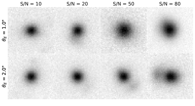
To account for seeing and sky-brightness variations over the course of the survey, each simulated exposure is drawn from a stochastic distribution of these parameters. We then consider two different strategies to use these exposures. For each field, we build one single-epoch image by keeping only the best seeing exposure and another “worst-case” stack image by co-adding all individual exposures after degrading them all in resolution to match the one with the worst seeing. These two sets of images will allow us to investigate the trade-off between signal-to-noise and resolution for our automated lens search.
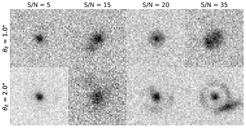
Examples of final mock observations with these two strategies are shown on Figure 5 for different arc sizes and signal to noise ratios (see Equation 9 for our definition of S/N). This ratio is defined in our final images in terms of the total flux of the lensed arc:
| (9) |
where is the total flux of the lensed source, is the rms noise in the observed image and is the number of pixels associated with the lensed source (measured by segmentation on a noiseless image of the arc using a threshold of , where is the rms noise in the corresponding full image.).
5 Results
In this section, we test the performance of our lens finder on the simulations described in the previous section. We perform these tests as a function of Einstein radius and S/N of the lensed source. For each class of simulations (single-epoch and stack), we train a model on a random subset of 16,000 images, following the procedure described in subsection 3.4. We then evaluate the performance of the classifier on a test set of 4,000 images as a function of various cuts in Einstein radius and S/N.
To quantify the performance of our lens finder, we measure the True Positive Rate (TPR) and False Positive Rate (FPR). The TPR, also known as completeness or recall, is defined as the ratio of detected lenses to the total number of lenses:
| (10) |
The FPR, which can also be interpreted as a contamination rate is defined as the fraction of non-lens images wrongly identified as lenses:
| (11) |
This statistic gives us a handle on the expected contamination of a lens sample while being independent of the ratio of lens to non-lens images in the testing set (not representative of a real survey in our simulations).
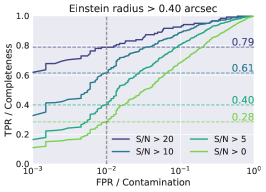
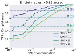
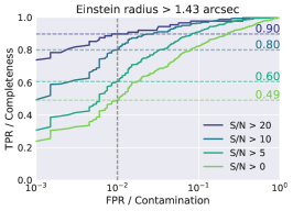
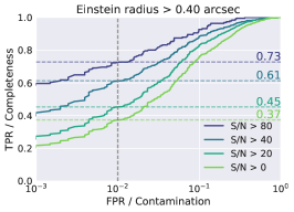
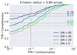
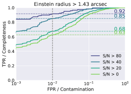
These statistics are a function of the detection threshold applied to the probability of an image containing a lens outputted by the model. This threshold balances completeness versus contamination of the lens sample. This trade-off is typically illustrated by the Receiver Operating Characteristic (ROC) curve which is obtained by plotting the TPR as a function of the FPR while varying this detection threshold from 0 to 1. Figure 6 shows the ROC curves of our classifier evaluated on the testing set, for various cuts in S/N and Einstein radius in the lens sample. We use a fiducial FPR value of 1% to derive a detection threshold for the rest of this analysis. This FPR value, illustrated by a vertical dashed line on Figure 6, would be set in practice based on what would be considered to be an admissible level of contamination in a given survey. The detection threshold corresponding to this FPR would then be derived from simulations.
For this fiducial detection level, we compare the corresponding completeness achieved by DeepLens for samples of increasingly larger and brighter arcs. These different completeness levels are marked by horizontal dashed lines on Figure 6.
We find that our lens finder exhibits very similar behaviour for the two sets of images. The increase in signal to noise seems to roughly compensate the loss in resolution. We note that in single exposure images, we achieve a completeness of 90% for our fiducial choice of 1% FPR, when considering arcs larger than ″. We reach similar completeness levels in stacked images for arcs of that size with S/N larger than 80.
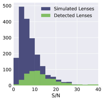
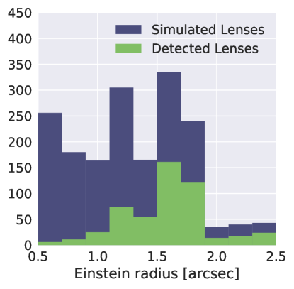
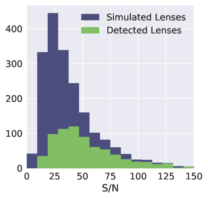
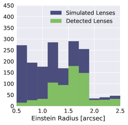
To further illustrate the impact of S/N and resolution on the recovery of lenses we show in Figure 7 the distributions of S/N and Einstein radius of our simulated lens population as well as the distribution of these properties in the recovered sample for our fiducial 1% FPR threshold. Interestingly, we find that in stacked images, DeepLens can still recover some poorly resolved lenses with Einstein Radius lower than the median seeing.
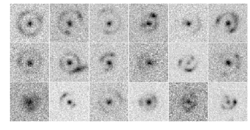
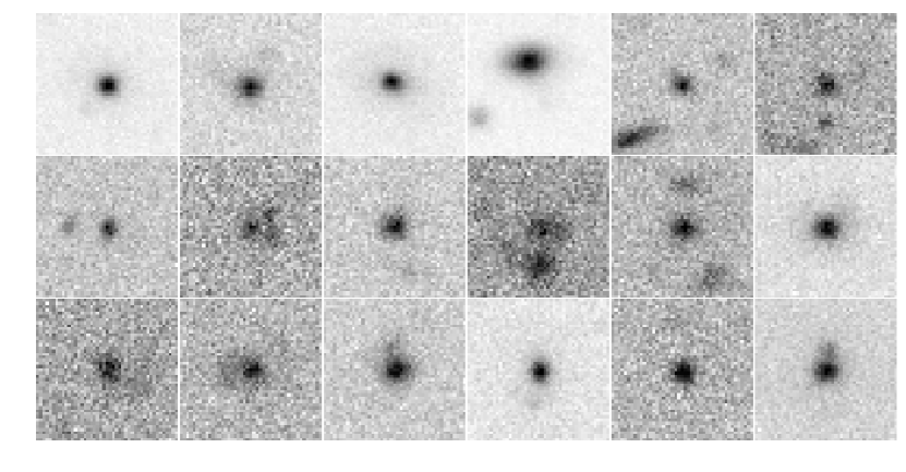
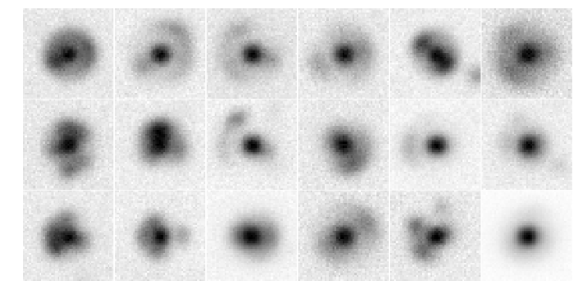
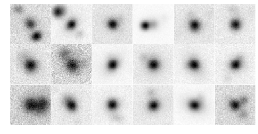
To visually investigate some failure modes of the model, we show on Figure 8 some examples of true and false positives for our two sets of simulations. We retain on this figure only the images with the highest predicted lens probability. As can be seen, the lenses for which DeepLens is the most certain have clearly visible rings and multiple images. False positives are dominated by the presence of multiple objects at the vicinity of the lens. We expect these types of failures to be dramatically reduced in multi-band images, as the colour would provide the necessary additional information to discriminate real lenses from these false positives.
6 Discussion
In this section we discuss the importance of simulations in a supervised machine learning method and provide several avenues to further improve our proposed model.
As in any supervised machine learning approach, the quality of the training set is a major factor in the performance of the method on actual data. For instance, Petrillo et al. (2017) find with a conventional CNN approach that most of the false positives that the method produces on real KiDS images come from contaminants such as ring galaxies, mergers or star-forming rings. For practical applications it is paramount to train Deep Learning models on representative datasets including all the diversity and variability of real survey images. We should therefore stress that the reported completeness and contamination levels on our simulations are only optimistic estimates of the performance of our model on real data.
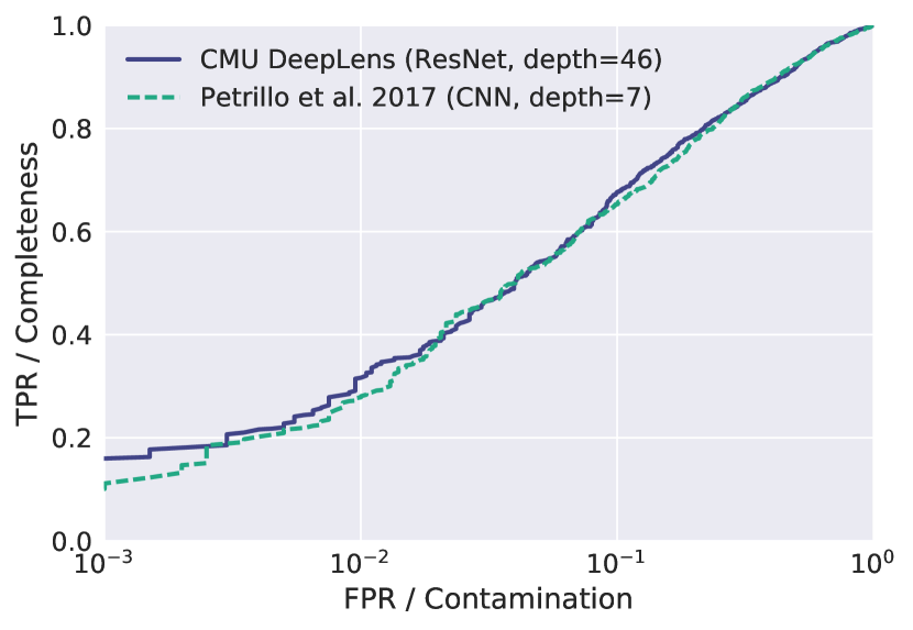
Realistic simulations are not only important for the final application to real data but also for method development. In particular we find that our simulations are not complex enough to discriminate between our proposed DeepLens model and a classical CNN model such as the one proposed in Petrillo et al. (2017), despite the greater complexity of our model (46 vs. 7 layers). As an illustration, we show on Figure 9 the ROC curve obtained by training and then evaluating a CNN following closely the description provided in Petrillo et al. (2017) on our set of simulations, along with the ROC curve obtained with our DeepLens model on the same training and testing set (single best epoch images). As can be seen, we find the two models to exhibit exactly the same performance when evaluated on our set of simulations, despite our model having outperformed most CNN based methods in the Euclid challenge (Metcalf et al. 2017, in prep.) and residual networks being known to significantly outperform CNNs in more complex image classification tasks (He et al., 2015a). This result shows that a simpler CNN is already complex enough to capture all the variability present in our non-trivial yet simple simulations, and no significant gains are made by increasing the complexity of the model. More complex simulations including more variability and non-trivial contaminants would reveal the limits of simpler models, whereas the additional complexity of a deeper model would facilitate a better interpretation of complex galaxy images to find robust features for lens detection. This result also illustrates the important point that when using supervised machine learning approaches, most of the burden is shifted from the development of the method itself to the production of realistic simulations for training purposes.
It should also be noted that we limited the complexity of our fiducial model to 46 layers but it can easily be made much deeper, and similar architectures have been successfully trained up to a thousand layers (He et al., 2016). There is still room for substantially more model complexity to handle more realistic simulations and data.
In the simulations presented in this work, we have only used single band images, which demonstrates our model’s ability to identify lenses from their morphologies alone. This is a valuable aspect of the method, especially for the Euclid survey, where lens searches will be conducted on the VIS single band images. However, colour information is also very helpful to identify strongly lensed systems and is already at the heart of some methods (e.g. Gavazzi et al., 2014). As mentioned in the description of our architecture, our model can seamlessly handle multi-band images and we expect its performance to be significantly improved by the addition of colour information.
Finally, we have only considered in this work generic galaxy-galaxy lenses. However a number of particularly interesting science cases require exotic lens systems such as double source plane lenses (e.g Collett & Auger, 2014), lensing catastrophes (Orban De Xivry & Marshall, 2009) or lensed SuperNovae (e.g. Rodney et al., 2016). However, these systems are much rarer and their specific detection is all the more challenging. In order to make our lens finder specifically sensitive to these rare cases, instead of a binary lens/non-lens classification, our method can be extended to a multi-class classification problem. A weighted cost function can also be used to further promote the purity of exotic lens candidates samples.
7 Conclusions
In this work, we presented CMU DeepLens, a new strong gravitational lens finder based on the most recent advances in Deep Learning. Our fully automated method does not require any manual tuning or human intervention beyond the training step. This new class of machine learning techniques represents an exciting prospect for conducting large-scale lens searches, as they have been shown to surpass human abilities in similar image classification tasks. They have the potential to significantly cut down on the need for human visual inspection and make the search for strong lenses tractable in the era of deep yet wide-field surveys such as LSST, Euclid and WFIRST. Being entirely automated, the selection function of such methods is also easier to quantify (given realistic simulations), which is a crucial point for precision cosmology (e.g. Collett & Cunnington, 2016).
We demonstrated on simple yet non-trivial strong lensing simulations of LSST -band observations that our algorithm is extremely efficient, rejecting a vast majority of non-lenses while preserving a high level of completeness. As a point of reference, we find that on single LSST exposures, for a fiducial rejection rate of 99%, we still reach a completeness of 90% for lenses with Einstein radii larger than and S/N of the lensed image larger than 20. We also investigated the trade-off between better S/N at the cost of lower resolution by applying our lens finder to co-added image stacks, degraded to the worst seeing in the stack. We find very similar performance in this case compared to single best seeing exposures. As a result we expect an optimal co-adding strategy to further improve on our results.
However, we note that these results are optimistic as our admittedly simple simulations do not include likely contaminants such as merging systems, spiral or ring galaxies. Our quoted completeness levels are therefore an optimistic estimate of the performance of our model on real data. We further demonstrate that our simulations are too simple to discriminate between deep learning models of vastly different complexities, meaning that a conventional CNN model exhibits the same performance as our more advanced and far deeper residual network model. On more realistic simulations however, such as the ones used for the strong lens finding challenge (Metcalf et al. 2017, in prep.), our residual network architecture was found to benefit from this added complexity and to outperform more conventional CNNs. This result illustrates the need for realistic simulations when developing and applying supervised machine learning methods, thus shifting part of the effort from the model development to the production of realistic simulations.
Finally, in the spirit of reproducible research, we make our code publicly available at https://github.com/McWilliamsCenter/CMUDeepLens .
The simulations used in this work will also be made available with an upcoming paper (Avestruz et al 2017, in prep).
Acknowledgements
The authors would like to acknowledge Michelle Ntampaka, Hy Trac, Phil Marshall, Frederic Courbin, Remy Joseph, Sukhdeep Singh, Noble Kennamer, and Siyu He for useful remarks and discussions. We also would like to acknowledge the Euclid Strong Gravitational Lensing Challenge and the Bologna Lens Factory project for fostering the development of automated strong lens finders. This research is supported in part by DOE grant DESC0011114 and NSF grant IIS1563887.
References
- Alard (2006) Alard C., 2006, preprint (arXiv:0606757)
- Auger et al. (2010) Auger M. W., Treu T., Bolton A. S., Gavazzi R., Koopmans L. V. E., Marshall P. J., Moustakas L. A., Burles S., 2010, The Astrophysical Journal, 724, 511
- Barnabè et al. (2011) Barnabè M., Czoske O., Koopmans L. V. E., Treu T., Bolton A. S., 2011, Monthly Notices of the Royal Astronomical Society, 415, 2215
- Bolton et al. (2006) Bolton A. S., Burles S., Koopmans L. V. E., Treu T., Moustakas L. A., 2006, The Astrophysical Journal, 638, 703
- Bom et al. (2017) Bom C. R., Makler M., Albuquerque M. P., Brandt C. H., 2017, Astronomy & Astrophysics, 597, A135
- Bonvin et al. (2017) Bonvin V., et al., 2017, Monthly Notices of the Royal Astronomical Society, 465, 4914
- Brault & Gavazzi (2015) Brault F., Gavazzi R., 2015, Astronomy & Astrophysics, 577, A85
- Cabanac et al. (2007) Cabanac R. A., et al., 2007, Astronomy and Astrophysics, 461, 813
- Cao et al. (2015) Cao S., Biesiada M., Gavazzi R., Piórkowska A., Zhu Z.-H., 2015, The Astrophysical Journal, 806, 185
- Clevert et al. (2015) Clevert D.-A., Unterthiner T., Hochreiter S., 2015, Under review of ICLR2016, 提出了ELU, pp 1–13
- Collett (2015) Collett T. E., 2015, The Astrophysical Journal, 811, 20
- Collett & Auger (2014) Collett T. E., Auger M. W., 2014, Monthly Notices of the Royal Astronomical Society, 443, 969
- Collett & Bacon (2016) Collett T. E., Bacon D. J., 2016, Monthly Notices of the Royal Astronomical Society, 456, 2210
- Collett & Cunnington (2016) Collett T. E., Cunnington S. D., 2016, Monthly Notices of the Royal Astronomical Society, 462, 3255
- Connolly et al. (2010) Connolly A. J., et al., 2010, SPIE Astronomical Telescopes + Instrumentation, pp 77381O–77381O–10
- Dieleman et al. (2015) Dieleman S., Willett K. W., Dambre J., 2015, Monthly Notices of the Royal Astronomical Society, 450, 1441
- Dye et al. (2008) Dye S., Evans N. W., Belokurov V., Warren S. J., Hewett P., 2008, Monthly Notices of the Royal Astronomical Society, 388, 384
- Galametz et al. (2013) Galametz A., et al., 2013, The Astrophysical Journal Supplement Series, 206, 10
- Gavazzi et al. (2007) Gavazzi R., Treu T., Rhodes J. D., Koopmans L. V. E., Bolton A. S., Burles S., Massey R. J., Moustakas L. A., 2007, The Astrophysical Journal, 667, 176
- Gavazzi et al. (2014) Gavazzi R., Marshall P. J., Treu T., Sonnenfeld A., 2014, The Astrophysical Journal, 785, 144
- Goodfellow et al. (2016) Goodfellow I., Bengio Y., Courville A., 2016, Deep learning. MIT Press (arXiv:1312.6184v5)
- Grogin et al. (2011) Grogin N. A., et al., 2011, The Astrophysical Journal Supplement Series December The Astrophysical Journal Supplement Series, 197, 3535
- He et al. (2015a) He K., Zhang X., Ren S., Sun J., 2015a, preprint, pp – (arXiv:1512.03385)
- He et al. (2015b) He K., Zhang X., Ren S., Sun J., 2015b, in 2015 IEEE International Conference on Computer Vision (ICCV). IEEE, pp 1026–1034 (arXiv:1502.01852), doi:10.1109/ICCV.2015.123, http://arxiv.org/abs/1502.01852http://ieeexplore.ieee.org/document/7410480/
- He et al. (2016) He K., Zhang X., Ren S., Sun J., 2016, preprint, pp 1–15 (arXiv:1603.05027)
- Hinton et al. (2012) Hinton G. E., Srivastava N., Krizhevsky A., Sutskever I., Salakhutdinov R. R., 2012, preprint, pp 1–18 (arXiv:1207.0580)
- Hornik et al. (1989) Hornik K., Stinchcombe M., White H., 1989, Neural Networks, 2, 359
- Hoyle (2016) Hoyle B., 2016, Astronomy and Computing, 16, 34
- Joseph et al. (2014) Joseph R., et al., 2014, Astronomy & Astrophysics, 566, A63
- Kim & Brunner (2017) Kim E. J., Brunner R. J., 2017, Monthly Notices of the Royal Astronomical Society, 464, 4463
- Kingma & Ba (2015) Kingma D. P., Ba J. L., 2015, International Conference on Learning Representations 2015, pp 1–15
- Koekemoer et al. (2011) Koekemoer A. M., et al., 2011, The Astrophysical Journal Supplement Series December The Astrophysical Journal Supplement Series, 197
- Koopmans et al. (2006) Koopmans L. V. E., Treu T., Bolton A. S., Burles S., Moustakas L. A., 2006, The Astrophysical Journal, 649, 599
- Krizhevsky et al. (2012) Krizhevsky A., Sutskever I., Hinton G. E., 2012, Advances In Neural Information Processing Systems, pp 1–9
- Kubo & Dell’Antonio (2008) Kubo J. M., Dell’Antonio I. P., 2008, Monthly Notices of the Royal Astronomical Society, 385, 918
- LSST Science Collaboration et al. (2009) LSST Science Collaboration et al., 2009, preprint, p. arXiv:0912.0201 (arXiv:0912.0201)
- Laureijs et al. (2011) Laureijs R., et al., 2011, preprint, p. arXiv:1110.3193 (arXiv:1110.3193)
- LeCun et al. (2015) LeCun Y., Bengio Y., Hinton G., 2015, Nature, 521, 436
- Lecun et al. (1998) Lecun Y., Bottou L., Bengio Y., Haffner P., 1998, Proceedings of the IEEE, 86, 2278
- Li et al. (2016) Li N., Gladders M. D., Rangel E. M., Florian M. K., Bleem L. E., Heitmann K., Habib S., Fasel P., 2016, The Astrophysical Journal, 828, 54
- Marshall et al. (2009) Marshall P. J., Hogg D. W., Moustakas L. A., Fassnacht C. D., Bradač M., Schrabback T., Blandford R. D., 2009, The Astrophysical Journal, 694, 924
- Marshall et al. (2015) Marshall P. J., et al., 2015, Monthly Notices of the Royal Astronomical Society, 455, 1171
- More et al. (2012) More A., Cabanac R., More S., Alard C., Limousin M., Kneib J.-P., Gavazzi R., Motta V., 2012, The Astrophysical Journal, 749, 38
- More et al. (2015) More A., et al., 2015, Monthly Notices of the Royal Astronomical Society, 455, 1191
- Nair & Hinton (2010) Nair V., Hinton G. E., 2010, Proceedings of the 27th International Conference on Machine Learning, pp 807–814
- Oguri & Marshall (2010) Oguri M., Marshall P. J., 2010, Monthly Notices of the Royal Astronomical Society, 405, 2579
- Orban De Xivry & Marshall (2009) Orban De Xivry G., Marshall P., 2009, Monthly Notices of the Royal Astronomical Society, 399, 2
- Petrillo et al. (2017) Petrillo C. E., et al., 2017, preprint, 19, 1 (arXiv:1702.07675)
- Ravanbakhsh et al. (2016) Ravanbakhsh S., Lanusse F., Mandelbaum R., Schneider J., Poczos B., 2016, preprint, pp 1–7 (arXiv:1609.05796)
- Refsdal (1964) Refsdal S., 1964, Monthly Notices of the Royal Astronomical Society, 128, 307
- Rodney et al. (2016) Rodney S. A., et al., 2016, The Astrophysical Journal, 820, 50
- Rumelhart et al. (1986) Rumelhart D. E., Hinton G. E., Williams R. J., 1986, Nature, 323, 533
- Seidel & Bartelmann (2007) Seidel G., Bartelmann M., 2007, Astronomy and Astrophysics, 472, 341
- Spergel et al. (2015) Spergel D., et al., 2015, preprint (arXiv:1503.03757)
- Srivastava et al. (2014) Srivastava N., Hinton G., Krizhevsky A., Sutskever I., Salakhutdinov R., 2014, Journal of Machine Learning Research, 15, 1929
- Suyu et al. (2010) Suyu S. H., Marshall P. J., Auger M. W., Hilbert S., Blandford R. D., Koopmans L. V. E., Fassnacht C. D., Treu T., 2010, The Astrophysical Journal, 711, 201
- Szegedy et al. (2015) Szegedy C., et al., 2015, Proceedings of the IEEE Computer Society Conference on Computer Vision and Pattern Recognition, 07-12-June, 1
- Treu (2010) Treu T., 2010, Annual Review of Astronomy and Astrophysics, 48, 87
- Zahid et al. (2015) Zahid H. J., Damjanov I., Geller M. J., Chilingarian I., 2015, The Astrophysical Journal, 806, 122
- de Jong et al. (2015) de Jong J. T. A., et al., 2015, Astronomy & Astrophysics, 582, A62