On Sampling from Massive Graph Streams

Abstract

We propose Graph Priority Sampling (gps), a new paradigm for order–based reservoir sampling from massive streams of graph edges. gps provides a general way to weight edge sampling according to auxiliary and/or size variables so as to accomplish various estimation goals of graph properties. In the context of subgraph counting, we show how edge sampling weights can be chosen so as to minimize the estimation variance of counts of specified sets of subgraphs. In distinction with many prior graph sampling schemes, gps separates the functions of edge sampling and subgraph estimation. We propose two estimation frameworks: (1) Post-Stream estimation, to allow gps to construct a reference sample of edges to support retrospective graph queries, and (2) In-Stream estimation, to allow gps to obtain lower variance estimates by incrementally updating the subgraph count estimates during stream processing. Unbiasedness of subgraph estimators is established through a new Martingale formulation of graph stream order sampling, which shows that subgraph estimators, written as a product of constituent edge estimators are unbiased, even when computed at different points in the stream. The separation of estimation and sampling enables significant resource savings relative to previous work. We illustrate our framework with applications to triangle and wedge counting. We perform a large-scale experimental study on real-world graphs from various domains and types. gps achieves high accuracy with $<1\%$ error for triangle and wedge counting, while storing a small fraction of the graph with average update times of a few microseconds per edge. Notably, for a large Twitter graph with more than 260M edges, gps accurately estimates triangle counts with $<1\%$ error, while storing only 40K edges.

1 Introduction

The rapid growth of the Internet and the explosion in online social media has led to a data deluge. A growing set of online applications are continuously generating data at unprecedented rates – these range from the Internet of things (e.g., connected devices, routers), electronic communication (e.g., email, groups, IMs, SMS), social media (e.g., blogs, web pages), to the vast collection of online social networks and content sharing applications (e.g., Facebook, Twitter, Youtube, Flickr). Graphs (networks) arise as a natural data representation in many of these application domains, where the nodes represent individuals (or entities) and the edges represent the interaction, communication, or connectivity among them.

These resulting interaction and activity networks carry a wealth of behavioral, community, and relationship information. Modeling and analyzing these massive and dynamic interaction graphs have become important in various domains. For example, detecting computer/terrorist attacks and anomalous behavior in computer networks and social media [8, 1], identifying the behavior and interests of users in online social networks (e.g., viral marketing, online advertising) [25, 41], monitoring and detecting virus outbreaks in human contact networks [26], among many others. But the volume and velocity of these graphs outpaces practitioners’ ability to analyze and extract knowledge from them. As a result, a common practice is to analyze static windowed snapshots of these graphs over time. However, this is costly and inefficient both in terms of storage volumes, and management for future use.

To keep up with the growing pace of this data, we need efficient methods to analyze dynamic interaction networks as the data arrives in streams, rather than static snapshots of graphs. In various application domains, graph mining is rapidly shifting from mining static graph snapshots to mining an open-ended graph stream of edges representing node interactions. We would like to have a framework capable of operating continuously and efficiently, processing edges/links as they arrive and providing timely answers for various network analysis tasks. This motivates the streaming graph model in which the graph is presented as a stream of edges/links in any arbitrary order, where each edge can be processed only once, and any computation uses a small memory footprint (i.e., often sub-linear in the size of the input stream) [29, 28, 5].

While studying dynamic interaction networks is important, other applications require efficient methods for the analysis of static graphs that are too large to fit in memory [35, 29]. In these cases traditional graph methods are not appropriate as they require random disk accesses that incur large I/O costs. This naturally leads to the question: how can we process massive static graphs sequentially (one edge at a time). The streaming graph model would provide an ideal framework for both massive static and dynamic graphs. It would also apply to the case of graph data that is stored as a list of edges streaming from storage. Thus, any algorithm designed to process graph streams is also applicable for static graphs [5].

Despite the recent advances in high-performance graph analysis tools and the availability of computational resources on the cloud, running brute-force graph analytics is usually too costly, too inefficient, and too slow in practical scenarios. In many cases, the cost of performing the exact computation is often not worth the extra accuracy. While an approximate answer to a query or an analysis task is usually sufficient, in particular when the approximation is performed with sufficient high-quality, unbiasedness, and confidence guarantees.

Sampling provides an attractive approach to quickly and efficiently find an approximate answer to a query, or more generally, any analysis objective. While previous work on sampling from graph streams focused on sampling schemes for the estimation of certain graph properties (i.e., in particular triangles) [23, 30, 10], in this paper however, we focus on an adaptive general purpose framework for sampling from graph streams. From a high-volume stream of edges, the proposed framework maintains a generic sample of limited size that can be used at any time to accurately estimate the total weight of arbitrary graph subsets (i.e., triangles, cliques, stars, subgraph with particular attributes). In order to obtain an accurate estimation of various graph properties, we need to maintain a weight sensitive sample that can devote sampling resources to edges that are informative for those properties.

In addition, we want a sampling scheme that is capable of utilizing auxiliary information about the items in the stream. Most of the previous work on stream sampling is either hard to adapt to various estimation objectives, focused on specific graph properties, or incapable of utilizing auxiliary information.

Contributions. The main contributions of this paper are as follows.

1. Framework. We propose graph priority sampling (gps), the first adaptive, general purpose, weight sensitive, one-pass, fixed-size without replacement sampling framework for massive graph streams. gps provides a general way to weight edge edge sampling according to auxiliary/size variables to estimate various graph properties (Sec 3). We discuss antecedents to our approach in Sec 2.

2. Theoretical Analysis. We provide a new Martingale formulation for subgraph count estimation, and show how to compute unbiased estimates of arbitrary subgraph counts from the sample at any point during the stream; we call this Post-Stream Estimation, which can be used to construct reference samples for retrospective graph queries (Sec 3).

3. In-Stream Estimation. We provide a second framework for In-stream Estimation in which subgraph count estimates are incrementally updated during stream processing rather than computed at a selected point, which can be used to obtain accurate estimates with lower variance (Sec 5).

4. Algorithms. We provide efficient/parallel algorithms for triangle and wedge count estimation using gps (Sec 4– 5).

5. Accuracy. We test our framework on graphs from various domains and types. Our estimates are accurate with $\leq 1\%$ error. Notably, for a large Twiiter graph with more than 260M edges, gps obtains an accurate estimate of triangle counts with $<1\%$ error, while storing only 40K edges (Sec 6).

6. Real-time Tracking. The proposed framework can maintain accurate real-time estimates while the stream is evolving (Sec 6).

We survey related work in Section 7 before concluding in Section 8. Proofs of the Theorems are deferred to Section 9.

2 Antecedents to Our Work

In this section, we highlight how our proposed framework generalizes many of the known sampling schemes. We discuss general statistical sampling schemes (reservoir sampling, probability proportional to size, order sampling), and highlight how graph priority sampling exploits the properties of these schemes.

Reservoir Sampling. Reservoir sampling is a class of single-pass sampling schemes to sample a fixed number $n$ (possibly weighted) items from a stream of $N>n$ items [24, 38]. The sample set is maintained incrementally over the stream, and can be used at any point in the stream to estimate the stream properties up to that point. In general, items have associated weight variables $w_{i}$ that determine non-uniform item inclusion probabilities $p_{i}$. Our graph priority sampling uses the reservoir sampling framework, to collect fixed-size weighted random sample from an input stream of edges using a single pass over the stream.

Probability Proportional to Size Sampling. In many real-world applications, an auxiliary variable (also known as a size or weight) is observed for each data item. Auxiliary variables correlated with the population variable under study can be used as weights for non-uniform sampling. In probability proportional to size sampling (PPS) the inclusion probability $p_{i}$ is proportional to the size (or weight) $w_{i}$. Variants of this scheme have been designed to fulfill different estimation goals [37]. Inclusion Probability Proportional to Size (IPPS) is variance minimizing for a given average sample size. It has marginal inclusion probabilities $p_{i}=\min\{1,w_{i}/\tau\}$, so that all items of weight $w_{i}$ below the threshold $\tau$ are sampled PPS, while larger items are always sampled [17]. Selected weights are assigned a Horvitz-Thompson [22] inverse probability unbiased estimator $\widehat{w}_{i}=w_{i}/p_{i}=\max\{w_{i},z\}$ if $w_{i}$ is selected, and implicitly $0$ otherwise. This property inspires the sampling weights used in our edge sampling scheme, which minimize the incremental estimation variance in the graph properties under study.

Order Sampling. In order (or rank-based) sampling, selection depends on random order variables generated for each item, a sample of size $m$ comprising the $m$ items of highest order. The distribution of the order variables is chosen to fulfill different weighted sampling objectives, including PPS sampling and Weighted Sampling without Replacement [31, 19, 13]. Priority Sampling [18] is a PPS scheme in which an item of weight $w_{i}$ is assigned a priority $w_{i}/u_{i}$, where the $u_{i}$ are IID uniform on $(0,1]$. A priority sample of size $n$ consists of the $n$ items of highest priority, and each selected item is assigned an unbiased estimator $\widehat{w}_{i}=\max\{w_{i},z\}$ of $w_{i}$, where $z$ is the $(n+1)^{\textrm{s}t}$ highest priority. Thus priority sampling resembles IPPS sampling with a random threshold.

Most of the above methods are suitable mainly for sampling IID data (e.g., streams of database transactions, IP network packets). In this paper, however, we are dealing with graph data, that exhibit both structure and attributes. A few of the methods discussed above have been extended to graph streams, in particular uniform-based reservoir sampling (see in Section 7). Graph priority sampling generalizes most of the above sampling schemes, and obtains an adaptive, weight sensitive, general purpose, fixed-size sample in one-pass, while including auxiliary/size variables representing topology information that we wish to estimate.

3 Graph Priority Sampling

This section establishes a methodological framework for graph stream priority sampling. Section 3.1 sets up our notation and states our estimation goals. Section 3.2 specifies the Graph Priority Sampling algorithm and states the properties that we will establish for it. Section 3.3 established unbiasedness for our subgraph estimators, while Section 3.4 gives unbiased estimates for the variance of these estimators. Section 3.5 shows how to choose sampling weight to minimize estimation variance for target subgraphs.

3.1 Proposed Framework

Notation and Problem Definition. Let $G=(V,K)$ be a graph with no self loops, where $V$ is the set of nodes, and $K$ is the set of edges. For any node $v\in V$, let $\Gamma(v)$ be the set of neighbors of node $v$ and so $\text{deg}(v)=|\Gamma(v)|$ is the degree of $v$. We call two edges $k,k^{\prime}\in K$ adjacent, $k\sim\ k^{\prime}$, if they join at some node, i.e., $k\;\cap\;k^{\prime}\neq\emptyset$ [3]. In this paper, we are principally concerned with estimating the frequency of occurrence of certain subgraphs of $G$. Our proposed graph stream model comprises an input graph $G=(V,K)$ whose edges arrive for sampling in any arbitrary order [3]. We assume edges are unique and so we can identify each edge in $K$ with its arrival order in $[|K|]=\{1,2,\dots,|K|\}$. Due to the identity between edges and arrival order we will use the notation $J\subset K$ and $J\subset[|K|]$ interchangeably. Thus, we can uniquely identify a subgraph $J\in{\mathcal{J}}$ with the corresponding ordered subset of edges $J\subset[|K|]$, written as an ordered subset, $J=({i_{1}},{i_{2}},...,{i_{\ell}})$ with $i_{1}<i_{2}<...<i_{\ell}$ being the arrival order. Thus, $J\subset[t]$ if all the edges in $J$ have arrived by time $t$.

We use the general notation ${\mathcal{J}}$ to denote the set of all subgraphs of $G$ whose count $N({\mathcal{J}})=|{\mathcal{J}}|$ we wish to estimate. As special cases, $\vartriangle$ will denote the set of triangles and $\Lambda$ the set of wedges (paths of length $2$) in $G$, Let $\alpha=3\cdot N(\vartriangle)/N(\Lambda)$ denote the global clustering coefficient of $G$. For a set of subgraphs ${\mathcal{J}}$ we shall use the notation ${\mathcal{J}}_{t}=\{J\in{\mathcal{J}}:J\subset[t]\}$ to denote those members $J$ of ${\mathcal{J}}$ all of whose edges have arrived by time $t$, The number of these is denoted $N_{t}({\mathcal{J}})=|{\mathcal{J}}_{t}|$

Algorithm and Intuition. The basic outline and intuition of the proposed framework comprises of two steps. In the first step, we select a small sample of edges $\widehat{K}_{t}\subset[t]$ from the set of all edges arriving by time $t$, with $m=|\widehat{K}_{t}|$ is the reservoir capacity. The second step allows us to estimate the count of general subgraphs in $G$ regardless of whether they were all sampled. We define the subset indicator of a subset of edges $J\subset[|K|]$ by the function,

$$S_{J,t}=\left\{\begin{array}[]{ll}1,&J\subset[t]\\ 0,&\mbox{otherwise}\\ \end{array}\right.$$ (1)

Thus, $S_{J,t}=1$ if and only if all the edges in $J$ have arrived by time $t$. In the above notation $S_{j,t}=N_{t}(\{j\})$ and $N_{t}({\mathcal{J}})=\sum_{J\in{\mathcal{J}}}S_{J,t}$ is the count of all members of ${\mathcal{J}}$ (i.e., subgraphs $J\in{\mathcal{J}}$) whose edges have all arrived by time $t$. Our goal is to estimate $N_{t}({\mathcal{J}})$ from a selected sample of edges $\widehat{K}_{t}\subset[t]$.

3.2 Algorithm Description & Properties

We formally state our main algorithm gps($m$) for Graph Priority Sampling into a reservoir $\widehat{K}$ of capacity $m$ in Algorithm 1. The main algorithm gps($m$) (see Algorithm 1) maintains a dynamic reservoir/sample $\widehat{K}$ of size $m$ from a graph whose edges are streaming over time. When a new edge $k$ arrives (Line 3), we call the procedure GPSupdate. We assume a weight function $W(k,\widehat{K})$ that expresses the sampling weight for edge $k$ as a function of both $k$ and the topology of the reservoir $\widehat{K}$ (Line 8). For example, $W(k,\widehat{K})$ could be set to the number of sampled edges adjacent to $k$, or the number of triangles in $\widehat{K}$ completed by $k$. In general, the function $W(k,\widehat{K})$ can be set to include topology, attributes, and/or any auxiliary information in the graph. Once the weight $w(k)=W(k,\widehat{K})$ is computed, we assign edge $k$ a priority $r(k)=w(k)/u(k)$ (Line 9), where $u(k)$ is an independent uniformly generated random number (Line 7). gps maintains a priority queue where each edge in the reservoir $\widehat{K}$ is associated with a priority (computed at arrival time) that defines its position in the heap. When a new edge $k$ arrives in the stream (and if the reservoir is full, see Lines 11–14), its priority is computed and compared with the lowest priority edge in the queue. If edge $k$ has a lower priority, then it is discarded. If edge $k$ has a higher priority, then the lowest priority edge is discarded and replaced by edge $k$.

Implementation and data structure. We implement the priority queue as a min-heap [14], where each edge has a priority less than or equal to its children in the heap, and the root position points to the edge with the lowest priority. Thus, access to the lowest priority edge is performed in $O(1)$. If edge $k$ has a higher priority than the root, edge $k$ is initially inserted at the root position, then moved downward to its correct position in the heap in $O(\log m)$ time (worst case). Note that if the sample size is less than the reservoir capacity, i.e., $|\widehat{K}|<m$, edge $k$ is inserted in the next available position in the heap, then moved upward to its correct position in the heap in $O(\log m)$ time (worst case). The threshold $z^{*}$ is the $(m+1)^{\text{st}}$ highest priority (see Line 13). To simplify the analysis, we provisionally admit a new edge $k$ to the reservoir, then one of the $m+1$ edges is discarded if it has the lowest priority. Finally, at any time in the stream, we can call the procedure GPSnormalize to obtain the edge sampling probabilities. As shown in the proof of Theorem 1, $p(k^{\prime})=\text{min}\{1,w(k^{\prime})/z^{*}\}$ (see Lines 16–17) is the conditional sampling probability for $k^{\prime}$ given $z^{*}$; hence $1/p(k^{\prime})$ forms the Horvitz-Thompson estimator for the indicator of $k^{\prime}$. The proposed framework gps naturally leads to a family of sampling algorithms that can be tuned for various graph sampling/analysis objectives. For example, if we set $W(k,\widehat{K})=1$ for every $k$, Algorithm 1 leads to uniform sampling as in the standard reservoir sampling (see [38]).

Algorithm 1   Family of Graph Priority Sampling Algorithms

1procedure GPS($m$)

2     $\widehat{K}\leftarrow\emptyset$; $z^{*}\leftarrow 0$

3     while new edge $k$ do

4         GPSupdate($k,m$)      

5     GPSnormalize($\widehat{K}$)  

6procedure GPSupdate($k,m$)

7     Generate $u(k)\sim\ Uni(0,1]$

8     $w(k)\leftarrow W(k,\widehat{K})$

9     $r(k)\leftarrow w(k)/u(k)$ $\triangleright$ Priority of edge $k$

10     $\widehat{K}\leftarrow\widehat{K}\cup\{k\}$ $\triangleright$ Provisionally include edge $k$

11     if $|\widehat{K}|>m$ then

12         $k^{*}\leftarrow\mathop{\mathrm{arg\,min}}_{k^{\prime}\in\widehat{K}}r(k^{\prime})$ $\triangleright$ Lowest priority edge

13         $z^{*}\leftarrow\max\{z^{*},r(k^{*})\}$ $\triangleright$ New threshold

14         $\widehat{K}\leftarrow\widehat{K}\setminus\{k^{*}\}$ $\triangleright$ Remove lowest priority edge       

15procedure GPSnormalize($\widehat{K}$)

16     for $k^{\prime}\in\widehat{K}$ do

17         $p(k^{\prime})\leftarrow\min\{1,w(k^{\prime})/z^{*}\}$ $\triangleright$ HT Renormalize      

Algorithm Properties. Graph Priority Sampling demonstrates the following properties: (S1) Fixed Size Sample. As seen above, $\widehat{K}_{t}$ is a reservoir sample of fixed size $|\widehat{K}_{t}|=m$ for all $t\geq m$.

(S2) Unbiased Subgraph Estimation. In Section 3.3 we construct unbiased subgraph estimators $\widehat{S}_{J,t}$ of $S_{J,t}$ for each subgraph $J$ and $t>0$. The $S_{J,t}$ is computable from the sample sets $\widehat{K}_{t}$. Section 5 extends our construction to new classes of estimators $\prod_{i\in J}\widehat{S}_{i,t_{i}}$ that are edge products over multiple times. These allow unbiased estimation of subgraphs in new ways: as they arise in the sample, or prior to discard, or on arrival of certain edges. These results follow from a novel Martingale formulation of graph priority sampling.

(S3) Weighted Sampling and Variance Optimization. Graph priority sampling provides a mechanism to tune sampling weights to the needs of applications. We accomplish this using edge weights that express the role of an edge in the sampled graph. Examples include the number of edges in the currently sampled graph that are adjacent to an arriving edge, and the number of subgraphs bearing a given motif that would be created by inclusion of the edge in the sample. Section 3.5 shows how to choose weights to minimize the variance of estimated counts of specific target subgraphs. Weights may also express intrinsic properties that do not depend explicitly on the graph structure. Examples include endpoint node/edge identities, attributes, and other auxiliary variables, such as user age, gender, interests, or relationship types in social networks, and bytes associated with communication links in technological/IP networks.

(S4) Computational Feasibility. For each arriving edge $k=(v_{1},v_{2})$, the gps framework calls GPSupdate to update reservoir $\widehat{K}$ of capacity $m$. The processing time for a new arrival comprises of the cost to compute the weight (i.e., $W(k,\widehat{K})$ and the cost to update the heap (if the new edge is inserted). We use a binary heap implemented by storing the edges in a standard array and using their relative positions within that array to represent heap (parent-child) relationships. The worst case cost of binary heap insertion/deletion is $O(\log m)$. The cost of $W(k,\widehat{K})$ is problem-specific and depends on the sampling objective and the function that computes the sampling weight for edge $k$. We use the number of triangles in $\widehat{K}$ completed by $k$, i.e., $W(k,\widehat{K})=|\widehat{\Gamma}(v_{1})\cap\widehat{\Gamma}(v_{2})|$. This can be achieved in $O(\text{min}\{\text{deg}(v_{1}),\text{deg}(v_{2})\})$, if a hash table or a bloom filter is used for storing $\widehat{\Gamma}(v_{1}),\widehat{\Gamma}(v_{2})$ and looping over the sampled neighborhood of the vertex with minimum degree and querying the hash table of the other vertex. The space requirements of gps is: $O(|\widehat{V}|+m)$, where $|\widehat{V}|$ is the number of nodes in the reservoir, and $m$ is the reservoir capacity. In general, there is a trade-off between space and time, and gps could limit the space to $O(m)$, however, the cost update per edge would require a pass over the reservoir ($O(m)$ in the worst case). On the other hand, if we increase the space to $O(|\widehat{V}|+m)$, then we can achieve a sub-linear time for edge updates.

3.3 A Martingale for Subgraph Counting

We now axiomatize the dependence of $w$ on $k$ and $\widehat{K}$ and analyze the statistical properties of estimates based on the sample set. We index edge arrivals by $t\in{\mathbb{N}}$, and let $\widehat{K}_{t}\subset[t]$ denote the set of indices in the sample after arrival $t$ has been processed and $\widehat{K}^{\prime}_{t}=\widehat{K}_{t-1}\cup\{t\}$ denote the index set after $t$ has been provisionally included in the sample. Let $w_{t}$ denote the weight assigned to arrival $t$ and $u_{t}$ be IID uniform on $(0,1]$. The priority of arrival $t$ is then $r_{t}=w_{t}/u_{t}$. An edge $i\in\widehat{K}^{\prime}_{t}$ is selected if it does not have the smallest priority in $\widehat{K}^{\prime}_{t}$, i.e., if

$$r_{i}>z_{i,t}=\min_{j\in\widehat{K}^{\prime}_{t}\setminus\{i\}}r_{j}$$ (2)

When $i$ is selected from $\widehat{K}^{\prime}_{t}$ then $r_{i,t}$ is equal to the unrestricted minimum priority $z_{t}=\max_{j\in\widehat{K}^{\prime}_{t}}r_{j}$ since the discarded edge takes the minimum. For $t<i$, $z_{i,t}=z_{t}$ since $i$ has not yet appeared. Defining $B_{i}(x)=\left\{r_{i}>x\right\}$, we write the event that $i$ is in the sample at time $t\geq i$ as

$$\{i\in\widehat{K}_{t}\}=\cap_{i=s}^{t}B_{i}(z_{i,s})$$ (3)

We now construct for each edge $i$ a sequence of Edge Estimators $\widehat{S}_{i,t}$ that are unbiased estimators of the corresponding edge indicators. We prove unbiasedness by establishing that the sequence is a Martingale  [39]. A sequence of random variables $\{X_{t}:t\in{\mathbb{N}}\}$ is a Martingale with respect to a filtration ${\mathcal{F}}=\{{\mathcal{F}}_{t}:t\in{\mathbb{N}}\}$ of increasing $\sigma$-algebra (these can be regarded as variables for conditioning) if each $X_{t}$ is measurable w.r.t. ${\mathcal{F}}_{t}$ (i.e. it is function of the the corresponding variables) and obeys:

$${\mathbb{E}}[X_{t}|{\mathcal{F}}_{t-1}]=X_{t-1}$$ (4)

Martingales provide a framework within which to express unbiased estimation in nested sequences of random variables.

We express gps within this framework. For $J\subset{\mathbb{N}}$ let $z_{J,t}=\min_{j\in\widehat{K}^{\prime}_{t}\setminus J}r_{j}$. Let ${\mathcal{F}}^{(0)}_{i,t}$ denote the $\sigma$-algebra generated by the variables $\{B_{j}(z_{\{ij\},s}):j\neq i,\ s\leq t\}$, let ${\mathcal{F}}_{i,t}$ be the $\sigma$-algebra generated by ${\mathcal{F}}^{(0)}_{i,t}$ and the variables ${\mathcal{Z}}_{i,t}=\{z_{i,s}:s\leq t\}$ and $\{B_{i}(z_{i,t}),i\leq s\leq t\}$, and let ${\mathcal{F}}_{i}$ be the filtration $\{{\mathcal{F}}_{i,t}:t\geq i-1\}$.

Set $z^{*}_{i,t}=\max_{i\leq s\leq t}z_{i,s}$ and define

$$R_{i,t}=\min\{1,w_{i}/z^{*}_{i,t}\}\mbox{ and }\widehat{S}_{i,t}=\frac{I(B_{i}(z^{*}_{i,t}))}{R_{i,t}}$$ (5)

for $t\geq i$ and $\widehat{S}_{i,t}=0$ for $0\leq t<i$.

Theorem 1 (Edge Estimation)

Assume $w_{i,t}$ is ${\mathcal{F}}_{i,t-1}$-measurable. Then $\{\widehat{S}_{i,t}:t\geq i\}$ is a Martingale w.r.t. the filtration ${\mathcal{F}}_{i}$, and hence ${\mathbb{E}}[\widehat{S}_{i,t}]=S_{i,t}$ for all $t\geq 0$

The measurability condition on $w_{i}$ means that it is determined by the previous arrivals, including the case that an edge weight depends on the sampled topology that it encounters on arrival.

To compute $\widehat{S}_{i}$ we observe that when $i\in\widehat{K}_{t}$, then (i) $r_{i}>z_{i,t}$ and hence $z_{i,t}=z_{t}$; and (ii) $z_{i,i}>\max_{s\leq i}z_{i,s}$ since otherwise the minimizing $j$ for $z_{i,i}$ could not have been selected. Hence for $t\geq i$ with $z^{*}_{t}=\max_{s\leq t}z_{s}$:

$$\widehat{S}_{i,t}=\frac{I(i\in\widehat{K}_{t})}{\min\{1,w_{i}/z^{*}_{t}\}}$$ (6)

It is attractive to posit the product $\widehat{S}_{J}=\prod_{i\in J}\widehat{S}_{i}$ as a subgraph estimator $J$ when $J\subset[t]$. While this estimator would be unbiased for independent sampling, the constraint of fixed-size introduces dependence between samples and hence bias of the product. For example, VarOpt sampling [12] obeys only ${\mathbb{E}}[\prod_{i\in J}\widehat{S}_{i}]\leq\prod_{i\in J}{\mathbb{E}}[\widehat{S}_{i}]$. We now show that the edge estimators for Graph Priority Sampling, while dependent, have zero correlation. This is a consequence of the property, that we now establish, that the edge product estimator is a Martingale.

Fix a subgraph as $J\subset{\mathbb{N}}$, set $J_{t}=J\cap[t]$ and for $k\in[t]\cap J^{c}$ define $z_{J,k,t}=\max_{i\in\widehat{K}^{\prime}_{t}\setminus(J_{t}\cup\{k\})}r_{i}$, i.e., the maximal rank in $\widehat{K}^{\prime}_{t}$ apart from $k$ and those in $J_{t}$. Let ${\mathcal{F}}^{(0)}_{J,t}$ denote the conditioning w.r.t $\{B_{k}(z_{J,k,s}):k\notin J,s\leq t\}$, and let ${\mathcal{F}}_{J,t}$ denote conditioning w.r.t ${\mathcal{F}}^{(0)}_{J,s}$, ${\mathcal{Z}}_{J,t}=\{z_{J,s}:s\leq t\}$ and $\{B_{i}(z_{J,s}):i\in J,s\leq t\}$ and let ${\mathcal{F}}_{J}$ denote the corresponding filtration.

Theorem 2 (Subgraph Estimation)

• For $J\subset{\mathbb{N}}$ define $S_{J,t}=\prod_{i\in J}\widehat{S}_{i,t}$. Then $\{\widehat{S}_{J,t}:t\geq\max J\}$ is a Martingale w.r.t. the filtration ${\mathcal{F}}_{J}$ and hence ${\mathbb{E}}[\prod_{i\in J}\widehat{S}_{i,t}]=S_{J,t}$ for $t\geq 0$.

• For any set ${\mathcal{J}}$ of subgraphs of $G$, $\widehat{N}_{t}({\mathcal{J}})=\sum_{J\in{\mathcal{J}}:J\subset K_{t}}\widehat{S}_{J,t}$ is an unbiased estimator of $N_{t}({\mathcal{J}})=|{\mathcal{J}}_{t}|=\sum_{J\in{\mathcal{J}}}S_{J,t}$, and the sum can be restricted to those $J\in{\mathcal{J}}$ for which $J\subset\widehat{K}_{t}$, i.e., entirely within the sample set at $t$.

The proof of Theorem 2(i) mirrors that of Theorem 1, and follows from the fact that the expectation of $\prod_{j\in J}B_{j}(z_{J,t})$, conditional on ${\mathcal{F}}_{J,t-1}$, is a product over $J$; we omit the details. Part (ii) follows by linearity of expectation, and the restriction of the sum follows since $\widehat{S}_{J,t}=0$ unless $J\subset\widehat{K}_{t}$.

3.4 Variance and Covariance Estimation

Theorem 2 also allows us to establish unbiased estimators for the variance and covariance amongst subgraph estimators. Consider two edge subsets $J_{1},J_{2}\subset\widehat{K}_{t}$. We use the following as an estimator of $\mathop{\mathrm{Cov}}(\widehat{S}_{J_{1},t},\widehat{S}_{J_{2},t})$:

$$\widehat{C}_{J_{1},J_{2},t} =\widehat{S}_{J_{1},t}\widehat{S}_{J_{2},t}-\widehat{S}_{J_{1}\setminus J_{2},t}\widehat{S}_{J_{2}\setminus J_{1},t}\widehat{S}_{J_{1}\cap J_{2},t}$$

$$=\widehat{S}_{J_{1}\setminus J_{2},t}\widehat{S}_{J_{2}\setminus J_{1},t}\widehat{S}_{J_{1}\cap J_{2},t}\bigg{(}\widehat{S}_{J_{1}\cap J_{2},t}-1\bigg{)}$$

$$=\widehat{S}_{J_{1}\cup J_{2},t}\bigg{(}\widehat{S}_{J_{1}\cap J_{2},t}-1\bigg{)}$$ (7)

Theorem 3 (Covariance Estimation)

$\widehat{C}_{J_{1},J_{2},t}$ is an estimator of $\mathop{\mathrm{Cov}}(\widehat{S}_{J_{1},t},\widehat{S}_{J_{2},t})$.

1. $\widehat{C}_{J_{1},J_{2},t}$ is an unbiased estimator of $\mathop{\mathrm{Cov}}(\widehat{S}_{J_{1},t},\widehat{S}_{J_{2},t})$.

2. $\widehat{C}_{J_{1},J_{2},t}\geq 0$ and hence $\mathop{\mathrm{Cov}}(\widehat{S}_{J_{1},t},\widehat{S}_{J_{2},t})\geq 0$.

3. $\widehat{S}_{J,t}(\widehat{S}_{J,t}-1)$ is an unbiased estimator of $\mathop{\mathrm{Var}}(\widehat{S}_{J,t})$.

4. $\widehat{C}_{J_{1},J_{2},t}=0$ if and only if $\widehat{S}_{J_{1},t}=0$ or $\widehat{S}_{J_{2},t}=0$, or $J_{1}\cap J_{2}=\emptyset$, i.e., covariance estimators are computed only from edge sets that have been sampled and their intersection is non-empty.

We do not provide the proof since these results are a special case of a more general result that we establish in Section 5 product form graph estimators in which the edges are sampled at different times.

3.5 Optimizing Subgraph Variance

How should the ranks $r_{i,t}$ be distributed in order to minimize the variance of the unbiased estimator $\widehat{N}_{t}({\mathcal{J}})$ in Theorem 2 ? This is difficult to formulate directly because the variances of the $\widehat{S}_{j,t}$ cannot be computed simply from the candidate edges. Instead, we minimize the conditional variance of the increment in $N_{t}({\mathcal{J}})$ incurred by admitting the new edge to the sample:

To be precise:

1. For each arriving edge $i$ find the marginal selection probability for $i$ that minimizes the conditional variance $\mathop{\mathrm{Var}}(\widehat{N}_{i}({\mathcal{J}})|{\mathcal{F}}_{i,i-1})$.

2. Edges are priority order sampled using weights that implement the variance-minimizing selection probabilities.

Our approach is inspired by the cost minimization approach of IPPS sampling [17]. When $i\in\widehat{K}^{\prime}_{t}$ we define $\widehat{N}_{i,t}({\mathcal{J}})=\#\{J\in{\mathcal{J}}:i\in J\wedge J\subset\widehat{K}^{\prime}_{t}\}$ i.e., the number of members $J$ of ${\mathcal{J}}$ that are subsets of the set of candidate edges $\widehat{K}^{\prime}_{t}$ and that contain $i$. Put another way, $\widehat{N}_{i,t}({\mathcal{J}})$ is the number of members of ${\mathcal{J}}$ that are created by including $i$ within $\widehat{K}_{t}$. Suppose $i$ is sampled with probability $p$, conditional on ${\mathcal{F}}_{i,i-1}$. The expected space cost of the sampled is proportional to $p$, while the sampling variance associated with Horvitz-Thompson estimation of the increment $n=\widehat{N}_{i,t}({\mathcal{J}})$ is $n^{2}(1/p-1)$. Following [17], we form a composite cost

$$C(z)=z^{2}p+n^{2}(1/p-1)$$ (8)

where $z$ is a coefficient expressing the relative scaling of the two components in the cost. $C(z)$ is minimized by $p=\min\{1,n/z\}$, corresponding to IPPS sampling with threshold $z$ and weight $n$. By comparison with the relation between threshold sampling and priority sampling, this suggests using $n=\widehat{N}_{i,t}({\mathcal{J}})$ as the weight for graph stream order sampling. We also add a default weight for each edge so that an arriving edge $k$ that does not currently intersect with the target class (i.e. $k\neq J\subset\widehat{N}_{t}({\mathcal{J}})$) can be sampled.

4 Triangle & Wedge Counting

In this section we apply the framework of Section 3 to triangle and wedge counting, and detail the computations involved for the unbiased subgraph count estimates and their variance estimates.

Unbiased Estimation of Triangle/Wedge Counts. From the notation in Sec. 3, let $\vartriangle_{t}$ denote the set of triangles whose all edges have arrived by time $t$, and $\widehat{\vartriangle}_{t}\subset\vartriangle_{t}$ be the subset of such triangles that appear in the sample $\widehat{K}_{t}$. Then, $\widehat{N}_{t}(\vartriangle)$ is the Horvitz-Thompson estimator of the count of members (i.e., triangles) in $\vartriangle_{t}$. We write $\tau\in\vartriangle_{t}$ as a subset $(k_{1},k_{2},k_{3})$ ordered by edge arrival (i.e., $k_{3}$ is the last edge). Similarly, $\Lambda_{t}$ denote the set of wedges whose all edges have arrived by time $t$. So $\widehat{N}_{t}(\Lambda)$ is the Horvitz-Thompson estimator of the count of wedges in $\Lambda_{t}$, and $\lambda\in\Lambda_{t}$ is written as an ordered subset $(k_{1},k_{2})$ with $k_{2}$ the last edge. The following are direct corollaries of Theorem 2:

Corollary 1 (Triangle Count)

$\widehat{N}_{t}(\vartriangle)=\sum_{\tau\in\vartriangle_{t}}\widehat{S}_{{\tau},t}$ is an unbiased estimator of $N_{t}(\vartriangle)$.

Corollary 2 (Wedge Count)

$\widehat{N}_{t}(\Lambda)=\sum_{\lambda\in\Lambda_{t}}\widehat{S}_{{\lambda},t}$ is an unbiased estimator of $N_{t}(\Lambda)$.

Additionally, we use $\widehat{\alpha}_{t}=3\widehat{N}_{t}(\vartriangle)/\widehat{N}_{t}(\Lambda)$ as an estimator for the global clustering coefficient $\alpha_{t}$.

Variance Estimation of Triangle/Wedge Counts. Let $\mathop{\mathrm{Var}}[\widehat{N}_{t}(\vartriangle)]$ denote the variance of the unbiased estimator of triangle count at time $t$, and $\mathop{\mathrm{Var}}[\widehat{N}_{t}(\Lambda)]$ the variance of the unbiased estimator of wedge count at time $t$, given by Corollaries 1 and 2 respectively. Expressions for unbiased estimates of these variances are direct corollaries from Theorem 3, which itself follows from Theorem 5.

Corollary 3 (Variance of Triangle Count)

$\widehat{V}_{t}(\vartriangle)$ is an unbiased estimator of $\mathrm{Var}[\widehat{N}_{t}(\vartriangle)]$, where

$$\widehat{V}_{t}(\vartriangle)=\sum\limits_{\tau\in\vartriangle_{t}}\widehat{S}_{{\tau},t}(\widehat{S}_{{\tau},t}-1)+2\sum\limits_{\tau\in\vartriangle_{t}}\sum\limits_{\begin{subarray}{c}\tau^{\prime}<\tau\\ \tau^{\prime}\in\vartriangle_{t}\end{subarray}}\widehat{C}_{\tau,\tau^{\prime},t}$$ (9)

Corollary 4 (Variance of Wedge Count)

$\widehat{V}_{t}(\Lambda)$ is an unbiased estimator of $\mathrm{Var}[\widehat{N}_{t}(\Lambda)]$, where

$$\widehat{V}_{t}(\Lambda)=\sum\limits_{\lambda\in\Lambda_{t}}\widehat{S}_{{\lambda},t}(\widehat{S}_{{\lambda},t}-1)+2\sum\limits_{\lambda\in\Lambda_{t}}\sum\limits_{\begin{subarray}{c}\lambda^{\prime}<\lambda\\ \lambda^{\prime}\in\Lambda_{t}\end{subarray}}\widehat{C}_{\lambda,\lambda^{\prime},t}$$ (10)

Variance Estimation for Global Clustering Coefficient. We use $\widehat{\alpha}=3\widehat{N}_{t}(\vartriangle)/\widehat{N}_{t}(\Lambda)$ as an estimate of the global clustering coefficient $\alpha=3N(\vartriangle)/N(\Lambda)$. While this estimate is biased, asymptotic convergence to the true value for large graphs would follow form the property for $\widehat{N}_{t}(\vartriangle)$ and $\widehat{N}_{t}(\Lambda)$. This motivates using a Taylor expansion of the estimator, using the asymptotic form of the well-known delta-method [36] in order to approximate its variance; see [3] for a similar approach for Graph Sample and Hold. The resulting approximation is:

$$\kern-10.0pt\mathop{\mathrm{Var}}(\widehat{N}(\vartriangle)/\widehat{N}(\Lambda))\kern-5.0pt \approx \kern-5.0pt\frac{\mathop{\mathrm{Var}}(\widehat{N}(\vartriangle))}{\widehat{N}(\Lambda)^{2}}+\frac{\widehat{N}(\vartriangle)^{2}\mathop{\mathrm{Var}}(\widehat{N}(\Lambda))}{\widehat{N}(\Lambda)^{4}}$$

$$-2\frac{\widehat{N}(\vartriangle)\mathop{\mathrm{Cov}}(\widehat{N}(\vartriangle),\widehat{N}(\Lambda))}{\widehat{N}(\Lambda)^{3}}$$

Following Theorem 3, the covariance $\mathop{\mathrm{Cov}}(\widehat{N}(\vartriangle),\widehat{N}(\Lambda))$ is estimated as

$$\widehat{V}(\vartriangle,\Lambda)=\sum_{\tau\in\widehat{\vartriangle},\lambda\in\widehat{\Lambda}\atop\tau\cap\lambda\neq\emptyset}\widehat{S}_{\tau\cup\lambda}\left(\widehat{S}_{\tau\cap\lambda}-1\right)$$ (12)

Efficiency. The basic intuition of Algorithm 2 is that the subgraph estimation problem is localized. Hence, all computations can be efficiently performed by exploring the local neighborhood of an edge (or a node) [6]. In this section, we discuss how the estimators can be adapted to make the computations more efficient and localized, while still remaining unbiased.

By linearity of expectation, we express the unbiased estimator $\widehat{N}_{t}(\vartriangle)$ (from Theorem 1) as $\widehat{N}_{t}(\vartriangle)=1/3\sum_{k\in\widehat{K}_{t}}\widehat{N}_{k,t}(\vartriangle)$ where $\widehat{N}_{k,t}(\vartriangle)$ is the conditional estimator of triangle counts for edge $k$ normalized by the number of edges in a triangle. Similarly, we express the unbiased estimator $\widehat{N}_{t}(\Lambda)$ (from Theorem 2) as $\widehat{N}_{t}(\Lambda)=1/2\sum_{k\in\widehat{K}_{t}}\widehat{N}_{k,t}(\Lambda)$ where $\widehat{N}_{k,t}(\Lambda)$ is the conditional estimator of wedge counts for edge $k$ normalized by the number of edges in a wedge.

Consider any two distinct edge subsets $J_{1},J_{2}\subset\widehat{K}_{t}$. From Theorem 3, the covariance estimator $\widehat{C}_{J_{1},J_{2},t}=0$ if $J_{1}$ and $J_{2}$ are disjoint (i.e., $|J_{1}\cap J_{2}|=0$). Otherwise, $\widehat{C}_{J_{1},J_{2},t}>0$ if and only if their intersection is non-empty (i.e., $|J_{1}\cap J_{2}|>1$). If $J_{1},J_{2}$ are triangles (or wedges), then $|J_{1}\cap J_{2}|\leq 1$, since any two distinct triangles (or wedges) could never overlap in more than one edge. Thus, the unbiased variance estimators can also be computed locally for each edge, as we show next.

By linearity of expectation, we re-write Equation 9 as follows:

$$\widehat{V}_{t}(\vartriangle) = 1/3\sum\limits_{k\in\widehat{K}_{t}}\sum\limits_{\tau\in\vartriangle_{t}(k)}\widehat{S}_{{\tau},t}(\widehat{S}_{{\tau},t}-1)$$

$$\kern-40.0pt+\sum\limits_{k\in\widehat{K}_{t}}\sum\limits_{\tau\in\vartriangle_{t}(k)}\sum\limits_{\begin{subarray}{c}\tau^{\prime}<\tau\\ \tau^{\prime}\in\vartriangle_{t}(k)\end{subarray}}\widehat{S}_{\tau\setminus\tau^{\prime},t}\widehat{S}_{\tau^{\prime}\setminus\tau,t}\widehat{S}_{\tau\cap\tau^{\prime},t}\bigg{(}\widehat{S}_{\tau\cap\tau^{\prime},t}-1\bigg{)}$$

Note that for any two distinct triangles $\tau,\tau^{\prime}\subset\widehat{K}_{t}$, we have $\widehat{S}_{\tau\cap\tau^{\prime},t}>0$ if and only if $\tau\cap\tau^{\prime}=\{k\}$ for some edge $k\in\widehat{K}_{t}$. Similarly, we could re-write Equation 10 as follows:

$$\widehat{V}_{t}(\Lambda) = 1/2\sum\limits_{k\in\widehat{K}_{t}}\sum\limits_{\lambda\in\Lambda(k)}\widehat{S}_{{\lambda},t}(\widehat{S}_{{\lambda},t}-1)$$

$$\kern-40.0pt+\sum\limits_{k\in\widehat{K}_{t}}\sum\limits_{\lambda\in\Lambda_{t}(k)}\sum\limits_{\begin{subarray}{c}\lambda^{\prime}<\lambda\\ \lambda^{\prime}\in\Lambda_{t}(k)\end{subarray}}\widehat{S}_{\lambda\setminus\lambda^{\prime},t}\widehat{S}_{\lambda^{\prime}\setminus\lambda,t}\widehat{S}_{\lambda\cap\lambda^{\prime},t}\bigg{(}\widehat{S}_{\lambda\cap\lambda^{\prime},t}-1\bigg{)}$$

Algorithm Description. To simplify the presentation of Algorithm 2, we drop the variable $t$ that denote the arrival time in the stream, however the algorithm is valid for any $t\in{\mathbb{N}}$. We start by calling Algorithm 1 to collect a weighted sample $\widehat{K}$ of capacity $m$ edges. For each edge $k\in\widehat{K}$, we use $W(k,\widehat{K})=9*|\widehat{\vartriangle}(k)|+1$ where $|\widehat{\vartriangle}(k)|$ is the number of triangles completed by edge $k$ and whose edges in $\widehat{K}$. Then, we call Algorithm 2 at any time $t$ in the stream to obtain unbiased estimates of triangle/wedge counts, global clustering, and their unbiased variance.

For each edge $k=(v_{1},v_{2})\in\widehat{K}$, Alg. 2 searches the neighborhood $\widehat{\Gamma}(v_{1})$ of the node with minimum degree (i.e., $\text{deg}(v_{1})\leq\text{deg}(v_{2})$ for triangles (Line 5). Lines 9–15 compute the estimates for each triangle $(k_{1},k_{2},k)$ incident to edge $k$. Lines 17–20 compute the estimates for each wedge $(k_{1},k)$ incident to edge $k$ (and centered on node $v_{1}$). Then, Lines 25–28 compute the estimates for each wedge $(k_{2},k)$ incident to edge $k$ (and centered on node $v_{2}$). Finally, the individual edge estimators are summed in Lines 32–36, and returned in Line 37.

We state two key observations in order: First, the estimators of triangle/wedge counts can be computed locally for each sampled edge $k\in\widehat{K}$, while still remaining unbiased. Thus, Algorithm 2 is localized. Second, since the estimators of triangle/wedge counts can be computed for each sampled edge $k\in\widehat{K}$ independently in parallel, Algorithm 2 already has abundant parallelism.

Complexity. Algorithm 2 has a total runtime of $O(m^{3/2})$. This is achieved by $\sum_{(v_{1},v_{2})\in\widehat{K}}{\text{min}\{\text{deg}(v_{1}),\text{deg}(v_{2})\})}=O(a(\widehat{K})m)$, where $a(\widehat{K})$ is the arboricity of the reservoir graph. This complexity can be tightly bounded by $O(m^{3/2})$ since $O(a(\widehat{K})m)\leq O(m^{3/2})$ for any sampled graph [11, 6].

Algorithm 2   Unbiased Estimation of Triangle & Wedge Counts

1procedure GPSestimate($\widehat{K}$)

2     Initialize all variables to zero

3     parallel for edge $k=(v_{1},v_{2})\in\widehat{K}$ do

4         $q\leftarrow\text{min}\{1,w(k)/z^{*}\}$

5         for each $v_{3}\in\widehat{\Gamma}(v_{1})$ do $\triangleright$ found wedge

6              $k_{1}\leftarrow(v_{1},v_{3})$

7              $q_{1}\leftarrow\text{min}\{1,w(k_{1})/z^{*}\}$

8              /*Compute triangle estimates*/

9              if $v_{3}\in\widehat{\Gamma}(v_{2})$ then $\triangleright$ found triangle

10                  $k_{2}\leftarrow(v_{2},v_{3})$

11                  $q_{2}\leftarrow\text{min}\{1,\w(k_{2})/z^{*}\}$

12                  $\widehat{N}_{k}(\vartriangle)\mathrel{+}=(qq_{1}q_{2})^{-1}$ $\triangleright$ triangle count

13                  $\widehat{V}_{k}(\vartriangle)\mathrel{+}=(qq_{1}q_{2})^{-1}((qq_{1}q_{2})^{-1}-1)$ $\triangleright$ tri. var.

14                  $\widehat{C}_{k}(\vartriangle)\mathrel{+}=c_{\vartriangle}*(q_{1}q_{2})^{-1}$ $\triangleright$ triangle covariance

15                  $c_{\vartriangle}=c_{\vartriangle}+(q_{1}q_{2})^{-1}$               

16              /*Compute wedge estimates for wedges $(v_{3},v_{1},v_{2})$*/

17              $\widehat{N}_{k}(\Lambda)\mathrel{+}=(qq_{1})^{-1}$ $\triangleright$ wedge count

18              $\widehat{V}_{k}(\Lambda)\mathrel{+}=(qq_{1})^{-1}((qq_{1})^{-1}-1)$ $\triangleright$ wedge variance

19              $\widehat{C}_{k}(\Lambda)\mathrel{+}=c_{\Lambda}*q_{1}^{-1}$ $\triangleright$ wedge covariance

20              $c_{\Lambda}=c_{\Lambda}+q_{1}^{-1}$          

21         /*Compute wedge estimates for wedges $(v_{3},v_{2},v_{1})$*/

22         for each $v_{3}\in\widehat{\Gamma}(v_{2})$ do

23              $k_{2}\leftarrow(v_{2},v_{3})$

24              $q_{2}\leftarrow\text{min}\{1,w(k_{2})/z^{*}\}$

25              $\widehat{N}_{k}(\Lambda)\mathrel{+}=(qq_{2})^{-1}$ $\triangleright$ wedge count

26              $\widehat{V}_{k}(\Lambda)\mathrel{+}=(qq_{2})^{-1}((qq_{2})^{-1}-1)$ $\triangleright$ wedge variance

27              $\widehat{C}_{k}(\Lambda)\mathrel{+}=c_{\Lambda}*q_{2}^{-1}$ $\triangleright$ wedge covariance

28              $c_{\Lambda}=c_{\Lambda}+q_{2}^{-1}$          

29         $\widehat{C}_{k}(\vartriangle)=\widehat{C}_{k}(\vartriangle)*2*q^{-1}*(q^{-1}-1)$

30         $\widehat{C}_{k}(\Lambda)=\widehat{C}_{k}(\Lambda)*2*q^{-1}*(q^{-1}-1)$      

31     /*Compute total triangle/wedge estimates*/

32     $\widehat{N}(\vartriangle)\leftarrow\frac{1}{3}*\sum_{k\in\widehat{K}}\widehat{N}_{k}(\vartriangle)$, $\widehat{N}(\Lambda)\leftarrow\frac{1}{2}*\sum_{k\in\widehat{K}}\widehat{N}_{k}(\Lambda)$

33     $\widehat{V}(\vartriangle)\leftarrow\frac{1}{3}*\sum_{k\in\widehat{K}}\widehat{V}_{k}(\vartriangle)$, $\widehat{V}(\Lambda)\leftarrow\frac{1}{2}*\sum_{k\in\widehat{K}}\widehat{V}_{k}(\Lambda)$

34     $\widehat{C}(\vartriangle)\leftarrow\sum_{k\in\widehat{K}}\widehat{C}_{k}(\vartriangle)$, $\widehat{C}(\Lambda)\leftarrow\sum_{k\in\widehat{K}}\widehat{C}_{k}(\Lambda)$

35     $\widehat{V}(\vartriangle)\leftarrow\widehat{V}(\vartriangle)+\widehat{C}(\vartriangle)$

36     $\widehat{V}(\Lambda)\leftarrow\widehat{V}(\Lambda)+\widehat{C}(\Lambda)$

37     return $\widehat{N}(\vartriangle),\widehat{N}(\Lambda),\widehat{V}(\vartriangle),\widehat{V}(\Lambda)$

5 In-Stream Estimation

The foregoing analysis enables retrospective subgraph queries: after any number $t$ of stream arrivals have taken place, we can compute an unbiased estimator $\widehat{S}_{t}(J$) for any subgraph $J$. We term this Post-Stream Estimation. We now describe a second estimation framework that we call In-Stream Estimation. In this paradigm, we can take “snapshots” of specific sampled subgraphs at arbitrary times during the stream, and preserve them as unbiased estimators. These can be used or combined to form desired estimators. These snapshots are not subject to further sampling; their estimates are not updated. However their original subgraphs remain in the graph sample and are subject to sampling in the normal way. Thus we do not change the evolution of the graph sample, we only extract information from it that does not change after extraction. The snapshot times need not be deterministic. For example, each time a subgraph that matches a specified motif appears (e.g. a triangle or other clique) we take a snapshot of the subgraph estimator. If we only need to estimate the number of such subgraphs, it suffices to add the inverse probability of each matching subgraph to a counter.

Algorithm 3 In-Stream Estimation of Triangle & Wedge Counts

1procedure Instream_GPS($K$)

2     $\widehat{K}\leftarrow\emptyset$; $z^{*}\leftarrow 0$

3     while new edge $k$ do

4         GPSestimate($k$)

5         GPSupdate($k,m$)      

6     return $\widetilde{N}(\vartriangle),\widetilde{N}(\Lambda),\widetilde{V}(\vartriangle),\widetilde{V}(\Lambda),\widetilde{V}(\vartriangle,\Lambda)$

7

8procedure GPSestimate($k$)

9     parallel for Triangle $(k_{1},k_{2},k)$ completed by $k$ do

10         if $(z^{*}==0)$ then $q_{1}\leftarrow q_{2}\leftarrow 1$

11         else

12              $q_{1}\leftarrow\min\{1,w(k_{1})/z^{*}\}$

13              $q_{2}\leftarrow\min\{1,w(k_{2})/z^{*}\}$          

14         $\widetilde{N}(\vartriangle)\mathrel{+}=1/(q_{1}q_{2})$$\triangleright$ Triangle Count

15         $\widetilde{V}(\vartriangle)\mathrel{+}=((q_{1}q_{2})^{-1}-1)/(q_{1}q_{2})$$\triangleright$ Triangle Var.

16         $\widetilde{V}(\vartriangle)\mathrel{+}=2(\widetilde{C}_{k_{1}}(\vartriangle)+\widetilde{C}_{k_{2}}(\vartriangle))/(q_{1}q_{2})$

17         $\widetilde{V}(\vartriangle,\Lambda)\mathrel{+}=(\widetilde{C}_{k_{1}}(\Lambda)+\widetilde{C}_{k_{2}}(\Lambda))/(q_{1}q_{2})$$\triangleright$ Tri.-Wedge Cov.

18         $\widetilde{C}_{k_{1}}(\vartriangle)\mathrel{+}=(q_{1}^{-1}-1)/q_{2}$$\triangleright$ Triangle Covariance

19         $\widetilde{C}_{k_{2}}(\vartriangle)\mathrel{+}=(q_{2}^{-1}-1)/q_{1}$      

20     parallel for Wedge $j\in\widehat{K}$ adjacent to $k$ do

21         if $(z^{*}==0)$ then $q\leftarrow 1$

22         else $q\leftarrow\min\{1,w(j)/z^{*}\}$          

23         $\widetilde{N}(\Lambda)\mathrel{+}=q^{-1}$$\triangleright$ Wedge Count

24         $\widetilde{V}(\Lambda)\mathrel{+}=q^{-1}(q^{-1}-1)$$\triangleright$ Wedge Variance

25         $\widetilde{V}(\Lambda)\mathrel{+}=2\widetilde{C}_{j}(\Lambda)/q$

26         $\widetilde{V}(\vartriangle,\Lambda)\mathrel{+}=\widetilde{C}_{j}(\vartriangle)/q$

27         $\widetilde{C}_{j}(\Lambda)\mathrel{+}=1/q-1$$\triangleright$ Wedge Covariance      

28

29procedure GPSupdate($k,m$)

30     Generate $u(k)$ uniformly on $(0,1]$

31     $w(k)\leftarrow W(k,\widehat{K})$

32     $r(k)\leftarrow w(k)/u(k)$ $\triangleright$ Priority of edge $k$

33     $\widehat{K}\leftarrow\widehat{K}\cup\{k\}$ $\triangleright$ Provisionally include edge $k$

34     $\widetilde{C}_{k}(\vartriangle)\leftarrow\widetilde{C}_{k}(\Lambda)\leftarrow 0$

35     if $|\widehat{K}|>m$ then

36         $k^{*}\leftarrow\mathop{\mathrm{arg\,min}}_{k^{\prime}\in\widehat{K}}r(k^{\prime})$ $\triangleright$ Lowest priority edge

37         $z^{*}\leftarrow\max\{z^{*},r(k^{*})\}$ $\triangleright$ New threshold

38         $\widehat{K}\leftarrow\widehat{K}\setminus\{k^{*}\}$ $\triangleright$ Remove lowest priority edge

39         $\widetilde{C}(\vartriangle)\leftarrow\widetilde{C}(\vartriangle)\setminus\widetilde{C}_{k^{*}}(\vartriangle)$ $\triangleright$ Remove covariances of $k^{*}$

40         $\widetilde{C}(\Lambda)\leftarrow\widetilde{C}(\Lambda)\setminus\widetilde{C}_{k^{*}}(\Lambda)$      

5.1 Unbiased Estimation with Snapshots

In-stream estimation can be described within the framework of stopped Martingales [39]. Return for the moment to our general description in Section 3 of a Martingale $\{X_{t}:t\in{\mathbb{N}}\}$ with respect to a filtration ${\mathcal{F}}=\{{\mathcal{F}}_{t}:t\in{\mathbb{N}}\}$. A random time $T$ is called a stopping time w.r.t ${\mathcal{F}}$ if the event $T\leq t$ is ${\mathcal{F}}_{t}$-measurable, i.e., we can decide at time $t$ whether the event has occurred yet. The corresponding stopped Martingale is

$$X^{T}=\{X^{T}_{t}:t\in{\mathbb{N}}\}\mbox{ where }X^{T}_{t}=X_{\min\{T,t\}}$$ (15)

Thus, the value of $X_{t}$ is frozen at $T$.

We define a snapshot as an edge subset $J\subset{\mathbb{N}}$ and a family $T=\{T_{j}:\ j\in J\}$ for ${\mathcal{F}}_{J}$-measurable stopping times, giving rise to the product stopped process

$$\widehat{S}^{T}_{J,t}=\prod_{j\in J}\widehat{S}^{T_{j}}_{j,t}=\prod_{j\in J}\widehat{S}_{j,\min\{T_{j},t\}}$$ (16)

Although in-steam estimates use snapshots whose edges have the same stopping time, variance estimation involves products of snapshots with distinct stopping times. Unbiasedness then follows from the following result that applies to any snapshot of the form (16).

Theorem 4

• $\{\widehat{S}^{T}_{J,t}:\ t\geq\max J\}$ is Martingale with respect to ${\mathcal{F}}_{J}$ and hence ${\mathbb{E}}[\widehat{S}_{J,t}^{T}]=S_{J,t}$.

• For any set ${\mathcal{J}}$ of subgraphs of $G$, each $J\subset{\mathcal{J}}$ equipped with an ${\mathcal{F}}_{J}$-measurable stoppong time $T_{J}$, then $\sum_{J\in{\mathcal{T}}_{j}}\widehat{S}^{T_{J}}_{J,t}$ is an unbiased estimator of $|{\mathcal{J}}_{t}|$.

5.2 Variance Estimation for Snapshots

In this section we show how the variance and covariances of snapshots can be estimated as sums of other snapshots involving the stopping times of both constituents. The Martingale formulation is a powerful tool to establish the unbiasedness of the estimates, since the otherwise statistical properties of the product of correlated edge estimators drawn at different times are not evident.

Consider two edge sets $J_{1}$ and $J_{2}$ each equipped with families stopping times $T^{(i)}=\{T^{(i)}_{j}:\ j\in J_{i}\}$, with $i=1,2$, for the purpose of snapshots. Thus each $j\in J_{1}\cap J_{2}$ is equipped with two generally distinct stopping times $T^{(1)}_{j}$ and $T^{(2)}_{j}$, according to its occurence in the snapshots $\widehat{S}^{T^{(1)}}_{J_{1},t}$ and $\widehat{S}^{T^{(2)}}_{J_{2},t}$. As an estimator of $\mathop{\mathrm{Cov}}(S^{T^{(1)}}_{J_{1},t},S^{T^{(2)}}_{J_{2},t})$ we will use:

$$\widehat{C}^{T^{(1)},T^{(2)}}_{J_{1},J_{2},t}=\widehat{S}^{T^{(1)}}_{J_{1},t}\widehat{S}^{T^{(2)}}_{J_{2},t}-\widehat{S}^{T^{(1)}}_{J_{1}\setminus J_{2},t}\widehat{S}^{T^{(2)}}_{J_{2}\setminus J_{1},t}\widehat{S}^{T^{(1)}\vee T^{(2)}}_{J_{1}\cap J_{2},t}$$ (17)

where $T^{(1)}\vee T^{(2)}=\{\max\{T^{(1)}_{j},T^{(2)}_{j}\}:\ j\in J_{1}\cap J_{2}\}$, i.e., we use the earlier stopping time for edges common to both subsets.

Theorem 5

• $\widehat{C}^{T^{(1)},T^{(2)}}_{J_{1},J_{2},t}$ is an unbiased estimator of $\mathop{\mathrm{Cov}}(\widehat{S}^{T^{(1)}}_{J_{1},t},\widehat{S}^{T^{(2)}}_{J_{2},t})$.

• $\widehat{C}^{T^{(1)},T^{(2)}}_{J_{1},J_{2},t}\geq 0$ and hence $\mathop{\mathrm{Cov}}(\widehat{S}^{T^{(1)}}_{J_{1},t},\widehat{S}^{T^{(2)}}_{J_{2},t})\geq 0$.

• $\widehat{S}^{T}_{J,t}(\widehat{S}^{T}_{J,t}-1)$ is an unbiased estimator of $\mathop{\mathrm{Var}}(\widehat{S}^{T}_{J,t})$.

• $\widehat{C}^{T^{(1)},T^{(2)}}_{J_{1},J_{2},t}=0$ if and only if $\widehat{S}^{T^{(1)}}_{J_{1},t}=0$ or $\widehat{S}^{T^{(2)}}_{J_{2},t}=0$, i.e., covariance estimators are computed only from snapshots that have been sampled.

Covariance Estimation for Post-Stream Sampling. Post-stream sampling is a special case of in-stream sampling with all $T_{j}=\infty$. We recover the corresponding Thm 3 concerning covariances from Theorem 5 by omitting all stopping times $T_{j}$ from the notation.

5.3 In-Stream Triangle & Wedge Counts

We now describe an application of In-Stream Estimation to Triangle Sampling and Counting. We sample from the stream based on the previous triangle count weighting, but the triangle counting is performed entirely in-stream. The full process is described in Algorithm 3. In this section we state and prove the form of estimators for triangle count and its variance, and describe the corresponding steps in the algorithm. Space limitations preclude giving a similar level of detail for wedge counting and triangle-wedge covariance.

Unbiased In-Stream Estimation of Triangle Count. Using our previous notation $\vartriangle_{t}$ to denote the set of triangles all of whose edges have arrived by $t$, we write each such triangle in the form $(k_{1},k_{2},k_{3})$ with $k_{3}$ the last edge to arrive. If $k_{1}$ and $k_{2}$ are present in the sample $\widehat{K}$ when $k_{3}$ arrives, we take a snapshot of the wedge $(k_{1},k_{2})$ prior to the sampling step for $k_{3}$. Formally, we let $T_{k_{3}}$ denote the slot immediately prior the arrival of $k_{3}$ and form the snapshot $\widehat{S}^{T_{k_{3}}}_{\{k_{1},k_{2}\}}$. Note $T_{k_{3}}$ is a stopping time because the edge arrival process is deterministic.

Theorem 6

$\widetilde{N}_{t}(\vartriangle)=\sum_{(k_{1},k_{2},k_{3})\in\vartriangle_{t}}\widehat{S}^{T_{k_{3}}}_{\{k_{1},k_{2}\},t}$ is an unbiased estimator of $N_{t}(\vartriangle)$.

Estimation of Triangle Count Variance. We add some further notation in preparation for estimating the variance of $\widetilde{N}_{t}(\vartriangle)$. Let $\widehat{K}_{[t]}=\cup_{t>0}\widehat{K}_{t}$ denote the set of edges that are sampled at any time up to $t$. Let $\widehat{\vartriangle}_{t}=\{(k_{1},k_{2},k_{3})\in\vartriangle_{t}:\widehat{S}_{\{k_{1},k_{2}\}}^{T_{k_{3}}}>0$} denote the (random) subset of all triangles in $\vartriangle_{t}$ that have positive snapshot. Let $\widehat{K}^{(2)}_{[t]}(k)$ denote the set of pairs $(j^{\prime},k^{\prime})$ of edges in $\widehat{K}_{[t]}$ such that each of the edge pairs $(k,j^{\prime})$ and $(k,k^{\prime})$ are the first two edges in distinct triangles in $\widehat{\vartriangle}_{t}$, and with $(j^{\prime},k^{\prime})$ ordered by their stopping time of the third edges in these triangles, i.e., $T_{k,j^{\prime}}<T_{k,k^{\prime}}$.

Theorem 7

$\mathop{\mathrm{Var}}(\widetilde{N}_{t}(\vartriangle))$ has unbiased estimator

$$\widetilde{V}_{t}(\vartriangle)=\kern-10.0pt\sum_{(k_{1},k_{2},k_{3})\in\widehat{\vartriangle}_{t}}\frac{1}{p_{k_{1},T_{k_{3}}}p_{k_{2},T_{k_{3}}}}\left(\frac{1}{p_{k_{1},T_{k_{3}}}p_{k_{2},T_{k_{3}}}}-1\right)\kern-220.0pt$$

$$\kern-10.0pt+2\sum_{k\in\widehat{K}_{[t]}}\sum_{{(j^{\prime},k^{\prime})\in\atop\widehat{K}^{(2)}_{[t]}(k)}}\frac{1}{p_{k^{\prime},T_{k,k^{\prime}}}p_{j^{\prime},T_{k,j^{\prime}}}p_{k,T_{k,k^{\prime}}}}\left(\frac{1}{p_{k,T_{k,j^{\prime}}}}-1\right)$$

Description of Algorithm 3. We now describe the portions of Algorithm 3 relating the in-stream estimator $\widetilde{N}(\vartriangle)$ and $\widetilde{V}(\vartriangle)$. When an edge $k$ arrives, an update is performed for each triangle that $k$ completes (line  9). These updates can be performed in parallel because each such triangle must have distinct edges other than $k$. Triangle count $\widetilde{N}(\vartriangle)$ is updated with the current inverse probabilities of its first two edges $k_{1}$ and $k_{2}$ (line 14). The variance $\widetilde{V}(\vartriangle)$ is updated first with the variance term for the current triangle (line 15) then secondly with its cumulative contributions $\widehat{C}_{k_{1}}(\vartriangle)$ and $\widehat{C}_{k_{1}}(\vartriangle)$ to the covariances with all previous triangles whose first two edges include $k_{1}$ or $k_{2}$ (line 16). These cumulative terms are then updated by the current triangle (lines  18 and  19). Wedge count variables are updated in a similar manner in lines 20–27. The edge-wedge covariance $\widetilde{V}(\vartriangle,\Lambda)$ used for estimation of the global clustering coefficient $\alpha$ is updated using the cumulative triangle and wedge covariances in lines 17 and 26.

6 Experiments and Results

We test the performance of graph priority sampling on a large set of $50$ graphs with hundreds of millions of nodes/edges, selected from a variety of domains and types, such as social, web, among others. All graph data sets are available for download  [33, 34]. For all graph datasets, we consider an undirected, unweighted, simplified graph without self loops. We generate the graph stream by randomly permuting the set of edges in each graph. For each graph, we perform ten different experiments with sample sizes in the range of 10K–1M edges. We test gps as well as baseline methods using a single pass over the edge stream (such that each edge is processed once): both gps post and in-stream estimation randomly select the same set of edges with the same random seeds. Thus, the two methods only differ in the estimation procedure. For these experiments, we used a server with two Intel Xeon E5-2687W 3.1GHz CPUs. Each processor has 8 cores with 20MB of L3 cache and 256KB of L2 cache. The experimental setup is executed independently for each sample size as follows:

1. For each sample size $m$, Alg 1 collects an edge sample $\widehat{K}\subset K$.

2. We use Alg 2 for post stream estimation, where the estimates are obtained only from the sample. We use Alg 3 for in-stream estimation, where the estimates are updated incrementally in a single pass during the sampling process. Thus, both gps post and in-stream estimation use the same sample.

3. Given a sample $\widehat{K}\subset K$, we use the absolute relative error (ARE) $|{\mathbb{E}}[\widehat{X}]-X|/X$ to measure the deviation between the expected value of the estimates $\widehat{X}$ and the actual statistics $X$. We use $X$ to refer to triangle, wedge counts, or global clustering.

4. We compute the $95\%$ confidence bounds as $\widehat{X}\pm 1.96\sqrt{\mathop{\mathrm{Var}}[\widehat{X}]}$.

Table 1: Estimates of expected value and relative error using 200K edges for a representative set of 11 graphs. The graphlet statistic for the full graph is shown in the third column. LB and UB are 95% confidence lower and upper bounds, respectively.

						actual	gps in-stream						gps post stream
	graph			$|K|$	$\frac{|\widehat{K}|}{|K|}$	$X$	$\widehat{X}$	$\frac{|X-\widehat{X}|}{X}$		LB	UB		$\widehat{X}$	$\frac{|X-\widehat{X}|}{X}$		LB	UB
triangles	ca-hollywood-2009			56.3M	0.0036	4.9B	4.9B	0.0009		4.8B	5B		4.8B	0.0036		4.6B	5.1B
	com-amazon			925.8K	0.216	667.1K	667.2K	0.0001		658.5K	675.8K		666.8K	0.0004		653.6K	680K
	higgs-social-network			12.5M	0.016	83M	82.6M	0.0043		80.8M	84.4M		83.2M	0.0031		79.5M	87M
	soc-livejournal			27.9M	0.0072	83.5M	83.1M	0.0043		80.6M	85.7M		81.5M	0.0244		72M	91M
	soc-orkut			117.1M	0.0017	627.5M	625.8M	0.0028		601.4M	650.1M		614.8M	0.0203		396M	833.7M
	soc-twitter-2010			265M	0.0008	17.2B	17.3B	0.0009		16.8B	17.7B		17.3B	0.0027		13.3B	21.3B
	soc-youtube-snap			2.9M	0.0669	3M	3M	0.0004		2.9M	3.1M		3M	0.0003		2.9M	3.1M
	socfb-Penn94			1.3M	0.1468	7.2M	7.1M	0.0063		7M	7.2M		7.1M	0.0044		6.8M	7.5M
	socfb-Texas84			1.5M	0.1257	11.1M	11.1M	0.0011		10.9M	11.3M		11.1M	0.0013		10.4M	11.9M
	tech-as-skitter			11M	0.018	28.7M	28.5M	0.0081		27.7M	29.3M		28.3M	0.0141		26.5M	30.1M
	web-google			4.3M	0.0463	13.3M	13.4M	0.0034		13.2M	13.6M		13.4M	0.0078		13.1M	13.8M
wedges	ca-hollywood-2009			56.3M	0.0036	47.6B	47.5B	0.0011		47.3B	47.8B		47.5B	0.0026		46.9B	48.1B
	com-amazon			925.8K	0.216	9.7M	9.7M	0.0002		9.7M	9.8M		9.7M	0.0021		9.6M	9.9M
	higgs-social-network			12.5M	0.016	28.7B	28.7B	0.001		28.5B	28.9B		28.7B	0.0008		28.1B	29.3B
	soc-livejournal			27.9M	0.0072	1.7B	1.7B	0.0005		1.7B	1.8B		1.8B	0.0008		1.7B	1.8B
	soc-orkut			117.1M	0.0017	45.6B	45.5B	0.0016		45B	46B		45.5B	0.0009		44.3B	46.8B
	soc-twitter-2010			265M	0.0008	1.8T	1.8T	0.0002		1.8T	1.8T		1.8T	0.0016		1.7T	1.8T
	soc-youtube-snap			2.9M	0.0669	1.4B	1.4B	0.0035		1.4B	1.4B		1.4B	0.0084		1.4B	1.5B
	socfb-Penn94			1.3M	0.1468	220.1M	219.9M	0.001		217.7M	222.1M		219M	0.0051		211.7M	226.3M
	socfb-Texas84			1.5M	0.1257	335.7M	334.9M	0.0022		331.4M	338.5M		335.1M	0.0017		323M	347.2M
	tech-as-skitter			11M	0.018	16B	16B	0.0005		15.8B	16.1B		15.9B	0.0016		15.6B	16.3B
	web-google			4.3M	0.0463	727.4M	728.8M	0.002		721M	736.7M		732.2M	0.0066		711.8M	752.5M
clustering coeff. (cc)	ca-hollywood-2009			56.3M	0.0036	0.31	0.31	0.002		0.306	0.315		0.309	0.0009		0.295	0.323
	com-amazon			925.8K	0.216	0.205	0.205	$\mathbf{<}$10-4		0.203	0.208		0.205	0.0025		0.201	0.209
	higgs-social-network			12.5M	0.016	0.009	0.009	0.0034		0.008	0.009		0.009	0.0039		0.008	0.009
	soc-livejournal			27.9M	0.0072	0.139	0.139	0.0039		0.135	0.143		0.136	0.0252		0.12	0.151
	soc-orkut			117.1M	0.0017	0.041	0.041	0.0012		0.04	0.043		0.04	0.0193		0.026	0.055
	soc-twitter-2010			265M	0.0008	0.028	0.028	0.0012		0.028	0.029		0.028	0.0004		0.022	0.035
	soc-youtube-snap			2.9M	0.0669	0.006	0.006	0.0032		0.006	0.006		0.006	0.0088		0.006	0.007
	socfb-Penn94			1.3M	0.1468	0.098	0.098	0.0053		0.096	0.099		0.098	0.0008		0.093	0.104
	socfb-Texas84			1.5M	0.1257	0.1	0.1	0.0012		0.098	0.102		0.1	0.0031		0.093	0.107
	tech-as-skitter			11M	0.018	0.005	0.005	0.0076		0.005	0.006		0.005	0.0124		0.005	0.006
	web-google			4.3M	0.0463	0.055	0.055	0.0014		0.054	0.056		0.055	0.0013		0.053	0.057

Error Analysis and Confidence Bounds. Table 1 summarizes the main graph properties and provides a comparison between gps post stream and in-stream estimation for a variety of graphs at sample size $m=$ 200K edges. First, we observe that gps in-stream estimation has on average $<1\%$ relative error across most graphs. In addition, gps post stream estimation has on average $\leq 2\%$. Thus, both methods provide accurate estimates for large graphs with a small sample size. Table 1 also shows that the upper and lower bounds of gps in-stream estimation are smaller than those obtained using gps post stream estimation. We note that both methods are using the same sample. However, a key advantage for gps in-stream estimation versus gps post stream estimation is its ability to minimize the variance of the estimators. Thus, gps in-stream estimates are not only accurate but also have a small variance and tight confidence bounds.

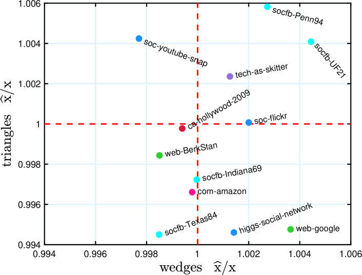
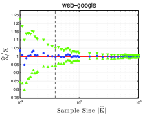
Second, we observe that the gps framework provides high quality general samples to accurately estimate various properties simultaneously. For example, Table 1 shows consistent performance across all graphs for the estimation of triangle/wedge counts and global clustering with the same sample. Similarly, in Figure 1, we observe that gps accurately estimates both triangle and wedge counts simultaneously with a single sample, with a relative error of $0.6\%$ for for both triangle and wedge counts.

Figure 1: Comparing $\nicefrac{{\widehat{x}}}{{x}}$ of triangles and wedges. The closer the points are to the intersection of the red lines (actual) the better. Points are colored by graph type. Results are from the in-stream estimation method at 100K.

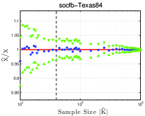
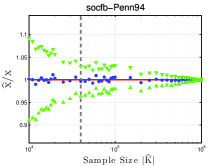
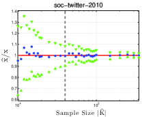
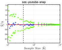
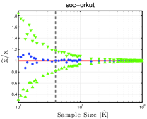
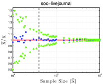
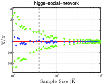
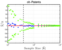
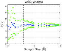
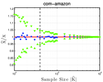
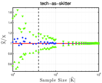
Finally, we investigate the properties of the sampling distribution and the convergence of the estimates as the sample size increases between 10K–1M edges (See Figure 2). We used graphs from various domains and types. We observe that the confidence intervals of triangle counts are small in the range $0.90$–$1.10$ for most graphs at 40K sample size. Notably, for a large Twitter graph with more than 260M edges (soc-twitter-10), gps in-stream estimation accurately estimates the triangle count with $<1\%$ error, while storing 40K edges, which is only a fraction of $0.00015$ of the total number of edges in the graph. Due to space limitations, we removed the confidence plots for wedges and clustering coefficient. However, we observe that the confidence interval are very small in the range of $0.98$–$1.02$ for wedges, and $0.90$–$1.10$ for global clustering coefficient.

Figure 2: Confidence bounds for Graph Priority Sampling with instream estimation of triangle counts. We used graphs from a variety of domains and types. The properties of the sampling distribution and convergence of the estimates are investigated as the sample size increases. The circle ($\newmoon$) represents $\nicefrac{{\widehat{X}}}{{X}}$ (y-axis) whereas $\blacktriangle$ and $\blacktriangledown$ are $\nicefrac{{LB}}{{X}}$ and $\nicefrac{{UB}}{{X}}$, respectively. Dashed vertical line (grey) refers to the sample at $40$K edges. Notably, the proposed framework has excellent accuracy even at this small sample size.

Table 2: Baseline Comparison at sample size $\approx$100K

	Nsamp	TRIEST	MASCOT	GPS Post
	Absolute Relative Error (ARE)
cit-Patents	$0.192$	$0.401$	$0.65$	$0.008$
higgs-soc-net	$0.079$	$0.174$	$0.209$	$0.011$
infra-roadNet-CA	$0.165$	$0.301$	$0.39$	$0.013$
	Average Time ($\mu_{s}$/edge)
cit-Patents	$34.2$	$3.01$	$2.02$	$0.63$
higgs-soc-net	$26.08$	$4.40$	$2.02$	$11.74$
infra-roadNet-CA	$28.72$	$2.81$	$2.05$	$0.831$

Baseline Study. The state-of-the-art algorithms for triangle count estimation in adjacency graph streams are due to the neighborhood sampling (Nsamp) in [30] and the triangle sampling (TRIEST) in [16]. We discuss their performance in turn compared with gps post stream estimation. We also compare with MASCOT [27]. Table 2 summarizes the results of the comparison. Our implementation of the Nsamp [30] algorithm follows the description in the paper, which achieves a near-linear total time if and only if running in bulk-processing. Otherwise the algorithm is too slow and not practical even for medium size graphs with a total time of $\mathcal{O}(|K|r)$. Overall, gps post stream estimation achieves 98%–99% accuracy, while Nsamp achieves only 80%–84% accuracy for most graphs and 92% accuracy for higgs-soc-net graph. Our implementation of the TRIEST [16] algorithm follows the main approach in the paper. TRIEST was unable to produce a reasonable estimate showing only 60%–82% accuracy. Similarly, MASCOT achieves only 35%–79% accuracy. Thus, gps post stream estimation outperforms the three baseline methods. Table 2 also shows the average update time per edge (in microseconds). We note that gps post stream estimation achieves an average update time that is 35x–56x faster than Nsamp with bulk-processing (for cit-Patents and infra-roadNet-CA graphs and at least 2x faster for higgs-soc-net). TRIEST and MASCOT use an average of 3 and 2 microseconds/edge respectively. Note that we have also compared to other methods in [23] and [10] (results omitted for brevity). Even though the method in  [10] is fast, it fails to find a triangle most of the time, producing low quality estimates (mostly zero estimates). On the other hand, the method of [23] is too slow for extensive experiments with $\mathcal{O}(m)$ update complexity per edge (where $m$ is the reservoir size). gps post stream estimation achieves at least 10x accuracy improvement compared to their method. For this comparison, we first run MASCOT with approximately 100K edges, then we observe the actual sample size used by MASCOT and run all other methods with the observed sample size.

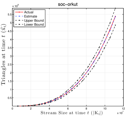
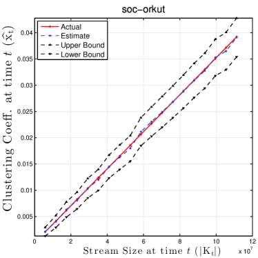
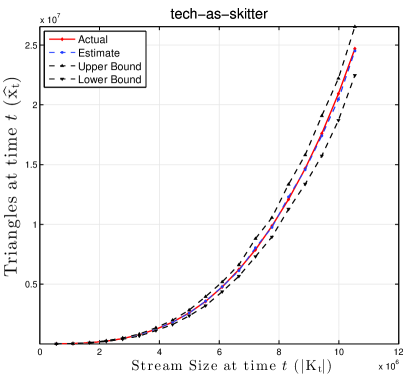
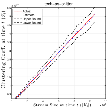
Unbiased Estimation Vs. Time. We now track the estimates as the graph stream progresses one edge at a time, starting from an empty graph. Figure 3 shows gps estimates for triangle counts and clustering coefficient as the stream is evolving overtime. Notably, the estimates are indistinguishable from the actual values. Figure 3 also shows the 95% confidence upper and lower bounds. These results are for a sample of 80K edges (a small fraction $\leq 1\%$ of the size of soc-orkut and tech-as-skitter graphs) using gps in-stream

Given the slow execution of Nsamp, we compare against TRIEST and its improved estimation procedure (TRIEST-Impr). Note that TRIEST and TRIEST-Impr are both using the same sample and random seeds. The two approaches are based on reservoir sampling [38]. We used graphs from a variety of domains and types for this comparison, and all methods are using the same sample size. We measure the error using the Mean Absolute Relative Error (MARE) $\frac{1}{T}\sum_{t=1}^{T}\frac{|\widehat{X}_{t}-X_{t}|}{X_{t}}$, where $T$ is the number of time-stamps. We also report the maximum error $\max_{t=1}^{T}\frac{|\widehat{X}_{t}-X_{t}|}{X_{t}}$. Table 3 summarizes the comparison results. For all graphs, gps with in-stream estimation outperforms both TRIEST and its improved estimation procedure TRIEST-Impr. We note that indeed TRIEST-Impr significantly improves the quality of the estimation of TRIEST. However, in comparison with gps  we observe that gps with post stream estimation is orders of magnitude better than TRIEST, which shows that the quality of the sample collected by gps is much better than TRIEST (regardless the estimation procedure used, whether it is post or in-stream estimation).

Figure 3: Graph Priority Sampling with in-stream estimation versus time. Results for social and tech networks at sample size 80K edges for triangle counts and global clustering with $95\%$ confidence lower and upper bounds. Notably, the proposed framework accurately estimates the statistics while the stream is progressing.

Scalability and Runtime. Our Algorithm 2 for post steam estimation uses a scalable parallel approach from [6, 7] with strong scaling properties; we omit the scalability results for brevity.

Table 3: Mean absolute relative error for estimates of triangle counts vs. time (sample size = 80K).

graph	Algorithm	Max. ARE	MARE
ca-hollywood-2009	TRIEST	$0.492$	$0.211$
	TRIEST-Impr	$0.066$	$0.018$
	GPS Post	$0.049$	$0.020$
	GPS in-stream	$0.016$	$0.003$
tech-as-skitter	TRIEST	$0.628$	$0.249$
	TRIEST-Impr	$0.134$	$0.048$
	GPS Post	$0.087$	$0.035$
	GPS in-stream	$0.032$	$0.014$
infra-roadNet-CA	TRIEST	$0.98$	$0.47$
	TRIEST-Impr	$0.33$	$0.09$
	GPS Post	$0.15$	$0.05$
	GPS in-stream	$0.058$	$0.02$
soc-youtube-snap	TRIEST	$0.362$	$0.119$
	TRIEST-Impr	$0.049$	$0.016$
	GPS Post	$0.022$	$0.009$
	GPS in-stream	$0.020$	$0.008$

7 Related Work

The research related to this paper can be grouped into: (a) Sampling from graph streams, (b) Sampling/Estimation of subgraphs.

Sampling from graph streams. Recently, there has been considerable interest in designing algorithms for mining massive and dynamic graphs from data streams, motivated by applications. Many were based on sampling and approximation techniques. An early such work [21] concerned problems of following paths and connectivity in directed graphs. Much of the earlier work on graph streams focused on graph problems in the semi-streaming model [29, 20], where the algorithm is allowed to use $\mathcal{O}(n\,\mathrm{polylog}\,n)$ space to solve graph problems that are provably intractable in sub-linear space. More recent work focused on graph mining problems such as finding common neighbors [9], estimation of pagerank [35], clustering and outlier detection [1], characterizing degree sequences in multigraph streams [15], link prediction [41], community detection [40], among others [28, 32, 2, 4]. See [5] for further details.

Sampling and Estimation of Subgraphs. Subgraph counting (in particular triangle counting) has gained significant attention due to its applications in social, information, and web networks. Early work in this direction [10] provides a space-bounded algorithm for the estimation of triangle counts and clustering coefficient in the incidence graph stream model. However, it has been shown that these guarantees will no longer hold in the case of the adjacency stream model, where the edges arrive in arbitrary order. A single pass streaming algorithm incurring $\mathcal{O}(m\Delta/T)$-space, where $\Delta$ is the maximum degree is proposed in [30]. However, this algorithm requires both large storage and update overhead to provide accurate results. For example, their algorithm needs at least $128$ estimators (i.e., storing more than $128$K edges) and uses large batch sizes (e.g., a million edges) to obtain accurate/efficient results. A single-pass $\mathcal{O}(m/\sqrt{T})$-space streaming algorithm was proposed in [23] specifically for transitivity estimation with arbitrary additive error guarantees. This algorithm maintains two reservoirs, the first to select a uniform sample of edges from the stream, and the second to select a uniform sample of wedges created by the edge reservoir.

Other approaches focused on maintaining a set of edges sampled randomly from the graph stream. graph sample-and-hold [3] is a framework for unbiased an accurate estimation of subgraph counts (e.g., edges, triangles, wedges). A similar approach was recently proposed for local (node/edge) triangle count estimation in graph streams [27]. Other methods extend reservoir sampling to graph streams. For example, reservoir sampling has been used for detecting outliers in graph streams [1], estimating the distribution of various graph properties (e.g., path length, clustering) [5], and estimating triangle counts in dynamic graph streams with insertions and deletions [16].

8 Conclusion

In this paper, we presented graph priority sampling, a new framework for order-based reservoir sampling from massive graph streams. gps provides a general way to weight edge sampling according to auxiliary variables to estimate various graph properties. We showed how edge sampling weights can be chosen so as to minimize the estimation variance of counts of subgraphs, such as triangles and wedges. Unlike previous graph sampling algorithms, gps differentiates between the functions of sampling and estimation. We proposed two estimation approaches: (1) Post-stream estimation, to allow gps to construct a reference sample of edges to support retrospective graph queries, and (2) In-stream estimation, to allow gps to obtain lower variance estimates by incrementally updating the count estimates during stream processing. We provided a novel Martingale formulation for subgraph count estimation. We performed a large-scale experimental analysis. The results show that gps achieves high accuracy with $<1\%$ error on large real-world graphs from a variety of domains and types, while storing a small fraction of the graph and average update times of a few microseconds per edge. In future work, we aim to extend the proposed approach to adaptive-weight sampling schemes and its applications in massive streaming analytics.

9 Proofs of Theorems

Lemma 5

For each $t$, the events $\left\{\{j\in K_{t}\}:j\leq t\right\}$ are measurable w.r.t ${\mathcal{F}}_{i,t}$ .

Proof 9.8 (of Lemma 5).

The proof is by induction. It is trivially true fot $t=i$. Assume true for $t-1$, then membership of $K_{t-1}$ is ${\mathcal{F}}_{i,t-1}$ measurable, and hence so is membership of $K^{\prime}_{t-1}$. Selection of $i$ is clearly ${\mathcal{F}}_{i,t}$-measurable, and if $i$ is selected, the remaining selections are ${\mathcal{F}}^{(0)}_{i,t}$-measurable since then $z_{\{ij\},t}=z_{j,t}$.

Proof 9.9 (of Theorem 1).

Lemma 5 established measurability.
For $t\geq i$, since $R_{i,t}$ is ${\mathcal{Z}}_{i,t}$-measurable, conditioning first on $z_{i,t}$:

$${\mathbb{E}}[\widehat{S}_{i,t}|z_{i,t},{\mathcal{F}}_{i,t-1}]=\frac{1}{R_{i,t}}{\mathbb{E}}[I(B_{i}(z^{*}_{i,t}))|z_{i,t},{\mathcal{F}}_{i,t-1}]$$ (19)

Since $B_{i}(z^{*}_{i,t})=B_{i}(z_{i,t})\cap B_{i}(z^{*}_{i,t-1})$ and $I(B_{i}(z^{*}_{t-1}))$ is ${\mathcal{F}}_{i,t-1}$-measurable, then for any event on which the conditional expectation (19) is positive, we have

$$\kern-25.0pt{\mathbb{E}}[I(B_{i}(z^{*}_{i,t}))|z_{i,t},{\mathcal{F}}_{i,t-1}]={\mathbb{P}}[B_{i}(z_{i,t})|B_{i}(z^{*}_{i,t-1}),{\mathcal{Z}}_{i,t},{\mathcal{F}}^{(0)}_{i,t-1}]$$ (20)

$$= {{\mathbb{P}}[B_{i}(z^{*}_{i,t})|{\mathcal{Z}}_{i,t},w_{i}]}/{{\mathbb{P}}[B_{i}(z^{*}_{i,t-1})|{\mathcal{Z}}_{i,t},w_{i}]}$$

$$= {{\mathbb{P}}[w_{i}/u_{i}>z^{*}_{i,t}|{\mathcal{Z}}_{i,t},w_{i}]}/{{\mathbb{P}}[w_{i}/u_{i}>z^{*}_{i,t-1}|{\mathcal{Z}}_{i,t},w_{i}]}$$

$$= R_{i,t}/R_{i,t-1}$$

where we have used the fact that once we have conditioned on $B_{i}(z^{*}_{i,t-1})$ and ${\mathcal{Z}}_{i,t}$, then ${\mathcal{F}}^{(0)}_{i,t-1}$ conditions only through the dependence of $w_{i}$ on the sample set $K_{i-1}$. Thus we have established that ${\mathbb{E}}[\widehat{S}_{i,t}|z_{i,t},{\mathcal{F}}_{i,t-1}]=\widehat{S}_{i,t-1}$ regardless of $z_{i,t}$, and hence ${\mathbb{E}}[\widehat{S}_{i,t}|{\mathcal{F}}_{i,t-1}]=\widehat{S}_{i,t-1}$.

Proof 9.10 (of Theorem 4).

(ii) follows from (i) by linearity of expectation. For (i), observe that $\widehat{S}^{T_{j}}_{j,t}=S^{T_{j}}_{j,t-1}+I(T\geq t)(\widehat{S}_{j,t}-\widehat{S}_{j,t-1})$; one checks that this reproduces $\widehat{S}_{j,\min\{t,T_{j}\}}$. Thus

$$\widehat{S}_{J,t}^{T}=\prod_{j\in J}\widehat{S}_{j,t-1}^{T_{j}}+\sum_{L\subsetneq J}\prod_{\ell\in L}S^{T_{\ell}}_{j,\ell-1}\kern-5.0pt\prod_{j\in J\setminus L}I(T_{j}\geq t)(\widehat{S}_{j,t}-\widehat{S}_{j,t-1})$$

Observe that $I(T_{j}\geq t)=1-I(T_{j}\leq t-1)$ is in fact ${\mathcal{F}}_{J,t-1}$-measurable. Hence taking expectations w.r.t. ${\mathcal{F}}_{J,t-1}$ then the product form from Theorem 2 tells us that for any $L\subsetneq J$

$${\mathbb{E}}[\prod_{j\in J\setminus L}I(T_{j}\geq t)(\widehat{S}_{j,t}-\widehat{S}_{j,t-1})|{\mathcal{F}}_{J,t-1}]\kern-150.0pt$$ (21)

$$= \prod_{j\in J\setminus L}I(T_{j}\geq t){\mathbb{E}}[\widehat{S}_{j,t}-\widehat{S}_{j,t-1}|{\mathcal{F}}_{J,t-1}]=0$$

and hence ${\mathbb{E}}[\widehat{S}_{J,t}^{T}|{\mathcal{F}}_{J,t-1}]=\prod_{j\in J}\widehat{S}_{j,t-1}^{T_{j}}=\widehat{S}_{J,t-1}^{T}$

Proof 9.11 (of Theorem 5).

(i)

$$\mathop{\mathrm{Cov}}(\widehat{S}^{T^{(1)}}_{J_{1},t},\widehat{S}^{T^{(2)}}_{J_{2},t}) = {\mathbb{E}}[\widehat{S}^{T^{(1)}}_{J_{1},t}\widehat{S}^{T^{(2)}}_{J_{2},t}]-{\mathbb{E}}[\widehat{S}^{T^{(1)}}_{J_{1},t}]{\mathbb{E}}[\widehat{S}^{T^{(2)}}_{J_{2},t}]$$ (22)

$$= {\mathbb{E}}[\widehat{S}^{T^{(1)}}_{J_{1},t}S^{T^{(2)}}_{J_{2},t}]-1$$

Hence the results follows because

$$E[\widehat{S}^{T^{(1)}}_{J_{1}\setminus J_{2},t}\widehat{S}^{T^{(2)}}_{J_{2}\setminus J_{1},t}\widehat{S}^{T^{(1)}\vee T^{(2)}}_{J_{1}\cap J_{2},t}]=1$$ (23)

from Theorem 4 since $J_{1}\setminus J_{2}$, $J_{2}\setminus J_{1}$ and $J_{1}\cap J_{2}$ are disjoint.

(ii)$\widehat{C}^{T^{(1)},T^{(2)}}_{J_{1},J_{2},t}=\widehat{S}^{T^{(1)}}_{J_{1}\setminus J_{2},t}\widehat{S}^{T^{(2)}}_{J_{2}\setminus J_{1},t}(\widehat{S}^{T^{(1)}}_{J_{1}\cap J_{2}}\widehat{S}^{T^{(2)}}_{J_{1}\cap J_{2}}-\widehat{S}^{T^{(1)}\vee T^{(2)}}_{J_{1}\cap J_{2},t})$. which is nonnegative since each $j\in J_{1}\cap J_{2}$ brings a factor of the form $1/(p^{(1)}p^{(2)})$ to $\widehat{S}^{T^{(1)}}_{J_{1}\cap J_{2}}\widehat{S}^{T^{(2)}}_{J_{1}\cap J_{2}}$, where $p^{(i)}=p_{j,\max\{t,T^{(i)}_{j}\}}$. This exceeds the matching term in $\widehat{S}^{T^{(1)}\vee T^{(2)}}_{J_{1}\cap J_{2},t}$, i.e., $1/\min\{p_{1},p_{2}\}$.

(iii) Follows from (i) upon setting $J_{1}=J_{2}=J$.

(iv) The equivalence clearly applies to the first monomial in (17). For the second monomial, note that $(\widehat{S}^{T^{(1)}}_{J_{1},t}=0)\wedge(\widehat{S}^{T^{(2)}}_{J_{2},t}=0)$ if and only if $\widehat{S}^{T^{(1)}}_{j,t}=0$ for some $j\in J_{1}$ or $\widehat{S}^{T^{(2)}}_{j,t}=0$ for some $j\in J_{2}$. If this condition holds for some $j\in J_{1}\Delta J_{2}$ we are done. Otherwise, we require $\widehat{S}^{T^{(i)}_{j}}_{j,t}=0$ for some $j\in J_{1}\cap J_{2}$ and some $i\in\{1,2\}$. But for $j\in J_{1}\cap J_{2}$, $\widehat{S}^{T^{(i)}_{j}}_{j,t}=\widehat{S}_{j,\min\{T^{(i)}_{j},t\}}=0$ means that $j$ has not survived until $\min\{T^{(i)}_{j},t\}$ and hence it also not present at the later or equal time $\min\{\max\{T^{(1)}_{j}T^{(2)}_{j}\},t\}$. Hence $\widehat{S}^{\max\{T^{(1)}_{j},T^{(2)}_{j}\}}_{j,t}=0$ and we are done

Proof 9.12 (of Theorem 6).

$\widehat{S}^{T_{k_{3}}}_{\{k_{1},k_{2}\},t}>0$ only if $(k_{1},k_{2},k_{3})\in\Delta_{t}$, and by Theorem 4 has unit expectation.

Proof 9.13 (of Theorem 7).

Distributing the covariance over the
sum $\widetilde{N}_{t}(\vartriangle)$ in Theorem 6, $\mathop{\mathrm{Var}}(\widetilde{N}_{t}(\vartriangle))$ has unbiased estimator

$$\kern-5.0pt\sum_{(k_{1},k_{2},k_{3})\in\vartriangle_{t}}\kern-17.0pt\widehat{S}_{\{k_{1},k_{2}\},t}^{T_{k_{3}}}(\widehat{S}_{\{k_{1},k_{2}\},t}^{T_{k_{3}}}-1)+2\kern-15.0pt\sum_{{(k_{1},k_{2},k_{3})\prec\atop(k^{\prime}_{1},k^{\prime}_{2},k^{\prime}_{3})}}\kern-15.0ptC_{\{k_{1},k_{2}\},\{k_{1}^{\prime},k_{2}^{\prime}\},t}^{T_{k_{3}},T_{k^{\prime}_{3}}}$$ (24)

Where $\prec$ denotes $k_{3}<k^{\prime}_{3}$ in arrival order. Each variance term is of the form $1/q(1/q-1)$ for $q=p_{k_{1},T_{3}}p_{k_{2},T_{3}}$. Each covariance term is zero unless $\{k_{1},k_{2}\}\cap\{k^{\prime}_{1},k^{\prime}_{2}\}\neq\emptyset$. (The sets cannot be equal for then $k_{3}=k^{\prime}_{3}$ if both form triangles). The stated form the follows by rewriting the sum of covariance terms in (24) as a sum over edges $k\in\widetilde{K}_{t}$ of the covariances of all pairs snapshots that contain $k$ as a sampled edge.

References

- [1] C. Aggarwal, Y. Zhao, and P. Yu. Outlier detection in graph streams. In ICDE, pages 399–409, 2011.
- [2] N. K. Ahmed, F. Berchmans, J. Neville, and R. Kompella. Time-based sampling of social network activity graphs. In MLG, pages 1–9, 2010.
- [3] N. K. Ahmed, N. Duffield, J. Neville, and R. Kompella. Graph sample and hold: A framework for big-graph analytics. In SIGKDD, 2014.
- [4] N. K. Ahmed, J. Neville, and R. Kompella. Network sampling designs for relational classification. In ICWSM, pages 1–4, 2012.
- [5] N. K. Ahmed, J. Neville, and R. Kompella. Network sampling: From static to streaming graphs. In TKDD, 8(2):1–56, 2014.
- [6] N. K. Ahmed, J. Neville, R. A. Rossi, and N. Duffield. Efficient graphlet counting for large networks. In In ICDM.
- [7] N. K. Ahmed, J. Neville, R. A. Rossi, N. Duffield, and T. L. Willke. Graphlet decomposition: framework, algorithms, and applications. In KAIS, pages 1–32, 2016.
- [8] L. Becchetti, P. Boldi, C. Castillo, and A. Gionis. Efficient semi-streaming algorithms for local triangle counting in massive graphs. In Proc. of KDD, pages 16–24, 2008.
- [9] A. Buchsbaum, R. Giancarlo, and J. Westbrook. On finding common neighborhoods in massive graphs. Theoretical Computer Science, 299(1):707–718, 2003.
- [10] L. Buriol, G. Frahling, S. Leonardi, A. Marchetti-Spaccamela, and C. Sohler. Counting triangles in data streams. In PODS.
- [11] N. Chiba and T. Nishizeki. Arboricity and subgraph listing algorithms. SIAM J. on Computing, 14(1):210–223, 1985.
- [12] E. Cohen, N. Duffield, H. Kaplan, C. Lund, and M. Thorup. Efficient stream sampling for variance-optimal estimation of subset sums. SIAM J. Comput., 40(5):1402–1431, Sept. 2011.
- [13] E. Cohen and H. Kaplan. Summarizing data using bottom-k sketches. In PODC, 2007.
- [14] T. H. Cormen, C. Stein, R. L. Rivest, and C. E. Leiserson. Introduction to Algorithms. 2nd edition, 2001.
- [15] G. Cormode and S. Muthukrishnan. Space efficient mining of multigraph streams. In PODS, pages 271–282, 2005.
- [16] L. De Stefani, A. Epasto, M. Riondato, and E. Upfal. Triest: Counting local and global triangles in fully-dynamic streams with fixed memory size. In KDD, 2016.
- [17] N. Duffield, C. Lund, and M. Thorup. Learn more, sample less, control of volume and variance in network measurement. IEEE Trans. in Information Theory, 51(5):1756–1775, 2005.
- [18] N. Duffield, C. Lund, and M. Thorup. Priority sampling for estimation of arbitrary subset sums. JACM, 54(6):32, 2007.
- [19] P. S. Efraimidis and P. G. Spirakis. Weighted random sampling with a reservoir. IPL, 97(5):181–185, 2006.
- [20] J. Feigenbaum, S. Kannan, A. McGregor, S. Suri, and J. Zhang. On graph problems in a semi-streaming model. Theoretical Computer Science, 348(2):207–216, 2005.
- [21] M. Henzinger, P. Raghavan, and S. Rajagopalan. Computing on data streams. In External Memory Algorithms: Dimacs Workshop External Memory and Visualization, volume 50, page 107, 1999.
- [22] D. G. Horvitz and D. J. Thompson. A generalization of sampling without replacement from a finite universe. J. of the American Stat. Assoc., 47(260):663–685, 1952.
- [23] M. Jha, C. Seshadhri, and A. Pinar. A space efficient streaming algorithm for triangle counting using the birthday paradox. In In ACM SIGKDD, pages 589–597, 2013.
- [24] D. E. Knuth. The Art of Computer Programming, Vol. 2: Seminumerical Algorithms. Addison-Wesley, 1997.
- [25] J. Leskovec, L. A. Adamic, and B. A. Huberman. The dynamics of viral marketing. In TWEB, 1(1):5, 2007.
- [26] J. Leskovec, A. Krause, C. Guestrin, C. Faloutsos, J. VanBriesen, and N. Glance. Cost-effective outbreak detection in networks. In KDD, pages 420–429, 2007.
- [27] Y. Lim and U. Kang. Mascot: Memory-efficient and accurate sampling for counting local triangles in graph streams. In Proc. of SIGKDD, pages 685–694. ACM, 2015.
- [28] A. McGregor. Graph mining on streams. Encyclopedia of Database Systems, pages 1271–1275, 2009.
- [29] S. Muthukrishnan. Data streams: Algorithms and applications. Now Publishers Inc, 2005.
- [30] A. Pavan, K. Tangwongsan, S. Tirthapura, and K.-L. Wu. Counting and sampling triangles from a graph stream. Proc. of VLDB, 6(14):1870–1881, 2013.
- [31] B. Rosén. Asymptotic theory for successive sampling with varying probabilities without replacement, I. The Annals of Mathematical Statistics, 43(2):373–397, 1972.
- [32] R. Rossi and N. Ahmed. Role discovery in networks. TKDE, 2015.
- [33] R. A. Rossi and N. K. Ahmed. The network data repository with interactive graph analytics and visualization. In AAAI, 2015.
- [34] R. A. Rossi and N. K. Ahmed. An interactive data repository with visual analytics. SIGKDD Explor., 17(2):37–41, 2016.
- [35] A. D. Sarma, S. Gollapudi, and R. Panigrahy. Estimating PageRank on Graph Streams. In PODS, pages 69–78, 2008.
- [36] M. J. Schervish. Theory of Statistics. Springer, 1995.
- [37] Y. Tillé. Sampling Algorithms. Springer-Verlag.
- [38] J. S. Vitter. Random sampling with a reservoir. ACM Transactions on Mathematical Software, 11:37–57, 1985.
- [39] D. Williams. Probability with Martingales. Cambridge University Press, 1991.
- [40] A. Zakrzewska and D. A. Bader. Tracking local communities in streaming graphs with a dynamic algorithm. SNAM, 6(1):65, 2016.
- [41] P. Zhao, C. Aggarwal, and G. He. Link prediction in graph streams. In ICDE, pages 553–564, 2016.