Bootstrapped Graph Diffusions:
Exposing the Power of Nonlinearity

Abstract.

Graph-based semi-supervised learning (SSL) algorithms predict labels for all nodes based on provided labels of a small set of seed nodes. Classic methods capture the graph structure through some underlying diffusion process that propagates through the graph edges. Spectral diffusion, which includes personalized page rank and label propagation, propagates through random walks. Social diffusion propagates through shortest paths. A common ground to these diffusions is their linearity, which does not distinguish between contributions of few “strong” relations and many “weak” relations.

Recently, non-linear methods such as node embeddings and graph convolutional networks (GCN) demonstrated a large gain in quality for SSL tasks. These methods introduce multiple components and greatly vary on how the graph structure, seed label information, and other features are used.

We aim here to study the contribution of non-linearity, as an isolated ingredient, to the performance gain. To do so, we place classic linear graph diffusions in a self-training framework. Surprisingly, we observe that SSL using the resulting bootstrapped diffusions not only significantly improves over the respective non-bootstrapped baselines but also outperform state-of-the-art non-linear SSL methods. Moreover, since the self-training wrapper retains the scalability of the base method, we obtain both higher quality and better scalability.

1. Introduction

Graph data is prevalent and models entities (nodes) and the strong interactions between them (edges). The source of these graphs can naturally come with the provided interactions (social networks, views, likes, purchases, messages, links) or can be derived from metric data (embedded entities) by retaining only edges that correspond to closest neighbors.

A fundamental task arises when label information is available only for a small set of seed entities $(x_{j},\boldsymbol{y}_{j})$ $j\leq n_{\ell}$ and we are interested in learning labels for all other entities $x_{i}$ for $i\in(n_{\ell},n_{\ell}+n_{u}]$. See e.g. the surveys (SemiSupervisedLearning:2006, ; GraphSSLbook:2014, ). The learning uses some smoothness assumption that similarity derived from the graph structure implies similarity of labels. Often the graph structure is combined with other features by the learning algorithms.

Classic methods for semi-supervised learning and many other related fundamental graph tasks (clustering, centrality, influence) are based on some underlying diffusion process that propagates from a node or set of nodes through the edges of the graph. The diffusion defines dense fine affinity relations between nodes using the provided sparse set of strong interactions. With SSL, the affinity relation guides the label learning, for example, by a weighted aggregation of seed labels to obtain soft labels.

Most popular SSL methods can be interpreted through underlying spectral diffusions (Chung:Book97a, ), utilizing the graph Laplacian, graph cuts (BlumChawla:ICML2001, ; BlumLRR:ICML2004, ), and random walks. They include label propagation (ZhuGL:ICML2003, ), label propagation using the normalized graph Laplacian (ZhouBLWS:NIPS2004, ; LinCohen:ICWSM2008, ), and many variations. The methods are highly scalable and implemented using Jacobi iterations that roughly translate into repeated averaging over neighboring nodes. The algorithms are applied successfully to massive graphs with billions of edges (RaviDiao:AISTATS2016, ) using highly distributed platforms (pregel:sigmod2010, ).

Another class of graph diffusions, which we refer to here as social, underline classic social and economic models of centrality (Bavelas:HumanOrg1948, ; Sabidussi:psychometrika1966, ; Freeman:sn1979, ; BlochJackson:2007, ; CoKa:jcss07, ; Opsahl:2010, ), influence (KKT:KDD2003, ; GRLK:KDD2010, ; DSGZ:nips2013, ; timedinfluence:2015, ), and similarity (CDFGGW:COSN2013, ) of nodes. Social diffusion propagate along shortest-paths (distance diffusion) or reachability searches (reach diffusion). A powerful extension defines a generative model from a graph by randomizing the presence (with reach diffusion) or the length (with distance diffusion) of edges (KKT:KDD2003, ; GRLK:KDD2010, ; CDFGGW:COSN2013, ; DSGZ:nips2013, ; timedinfluence:2015, ) and then works with respective expectations. Social diffusion, inspired by the independent cascade model of (KKT:KDD2003, ) and the continuous time (distance-based) model of (GRLK:KDD2010, ; CDFGGW:COSN2013, ; DSGZ:nips2013, ; timedinfluence:2015, ) was recently adapted to SSL (semisupInf:2016, ). The proposed algorithms scale very well: For the simpler nearest-seed variant which matches each label to the closest seed node in each simulation of the randomized model we simply use small number of graph (Dijkstra) searches. The use of distance or reachability sketching based on (ECohen6f, ) allows for highly scalable label learning also over the sketched affinity matrix.

Both spectral and social diffusion based SSL models scale well even with a large number of labels, using heavy hitter sketches with label propagation (RaviDiao:AISTATS2016, ) or naturally with social diffusion using sketches. We interpret these methods as linear in the sense that the diffusion propagates from seeds through edges without amplifying strong signals or suppressing weak ones.

Recently proposed non-linear learning methods, based on node embeddings and graph convolutional networks, had impressive success in improving the quality of the learned labels. In particular, DeepWalk (deepwalk:KDD2014, ) applied the hugely successful word embedding framework of (Mikolov:NIPS13, ) to embed the graph nodes in a way that preserves the affinity relation defined by co-occurrence frequencies of pairs in short random walks: A softmax applied to inner products of embeddings approximates the frequency of the pair. A supervised learning algorithm is then trained on the embedding vectors and labels of seed nodes. Node2vec (node2vec:kdd2016, ) refined the approach using hyperparameters that tune the depth and breadth of the random walks. Another method, Planetoid, used a multi-layer neural network instead of a single softmax layer (Yang:ICML2016, ). With these methods, the lower-dimensional embeddings serve as a “low rank” representation of the affinity matrix and the softmax and neural network introduce non-linearities that emphasize larger inner products. Another successful proposal are Graph convolutional networks (GCN) (HenaffBL:2015, ; AtwoodT:NIPS2016, ; DefferrardBV:NIPS2016, ; KipfW:ICLR2017, ), which are neural networks with layers that follow the graph adjacency structure. Each layer applies a non-linear activation function, most often a sigmoid or ReLU, to the aggregate over neighbors.

This abundance of recent work introduced many new components and often at the same time: Low-rank embeddings, non-linear propagations, learning of weights of hidden layers (GCNs), learning of node weights (NandanwarM:kdd2016, ). These recent methods, however, while demonstrating improved labeling quality, do not scale as well as label propagation and methods based on social graph diffusions.

Our aim here is to isolate the main contributor(s) to the quality gain of the recent non-linear approaches and to seek methods that combine the scalability advantage of the simpler diffusion models with state of the art labeling quality.

We explore placing these “linear” diffusions in a self-training (bootstrapping) framework. Self-training is arguably the earliest approach to SSL, dating back five decades to Scudder (Scudder1965, ), and extensively studied by the NLP community (Yarowsky:ACL1995, ; Abney:CL2004, ; WhitneySarkar:ACL2012, ). The self-training framework can be viewed as a wrapper around a base learning algorithm. The base algorithm takes as input a set of labeled examples and makes predictions with associated margins or confidence scores for other examples. The wrapper applies the base algorithm in steps, where at the end of each step, the highest-confidence predictions are converted to become new labeled examples.

Our bootstrapped diffusions retain the high scalability of the base diffusions while introducing non-linearity that allows us to work with a richer class of models. In particular, with our base algorithms, “seed” examples have a special role that is not amplified by implied high-confidence predictions. Bootstrapping provides such amplification by promoting high-margin predictions to “seed” roles.

We perform experiments using linear diffusion models and their bootstrapped versions. We use classic Label propagation (ZhuGL:ICML2003, ), Label propagation using the normalized Laplacian (ZhouBLWS:NIPS2004, ), and nearest-seed, which is the simplest distance diffusion model (semisupInf:2016, ). We apply a very basic bootstrapping wrapper that works with a fixed fraction of highest-margin predictions in each step. We focus on a multi-class setting, where each node is a member of one class, even though most of the method can be extended to the multi-label setting.

We apply the different methods to benchmark data and seed sets used and made available by previous work (Yang:ICML2016, ; KipfW:ICLR2017, ). In particular, we use social, citation, and knowledge graph data sets. We compare the quality of the learned labels to state of the art baselines, including DeepWalk (deepwalk:KDD2014, ), node2vec (node2vec:kdd2016, ), Planetoid (Yang:ICML2016, ), and GCNs (KipfW:ICLR2017, ). We also perform more elaborate experiments on additional data and seed sets and on the well-studied planted partition (stochastic block) model (CondonKarp:2001, ) which is often used to understand the performance of clustering and community detection algorithms.

Our main focus is the quality of learning from the graph structure alone using diffused seed node labels. We observe that bootstrapped diffusions consistently improved the quality, by 1% to 12%, over the base diffusion, both for spectral and social and across types of graphs. The most surprising outcome was that prediction quality on benchmark data exceeded that of all recent non-linear methods.

The use of additional available node (or edge) features can significantly increase labeling quality but there are multiple ways to integrate them in the learning algorithm. We consider the use of the raw provided node features or smoothing them through a graph diffusion. A simple supervised learning algorithm is then trained on the (raw or diffused) feature vectors and class labels of seed nodes. We applied this method with and without bootstrapping. We observed that both diffusion and bootstrapping significantly enhanced performance. Furthermore, our results dominated those reported (with the use of node features) by the state of the art baselines Planetoid (Yang:ICML2016, ) and GCNs (KipfW:ICLR2017, ). In particular, GCNs lend themselves to a direct comparison as they can be viewed as a feature diffusion with non-linearities applied after each set of edge traverasals and node/layer weight tuned through back propagations. It is interesting that we obtained comparable or better results using bootstrapped linear models and without backprop training.

The paper is organized as follows. The linear base diffusion we use and the bootstrapping wrapper are discussed in Section 2. Our data sets and our experimental methodology are laid out in Section 3. The results on the benchmark data are reported and discussed in Section 4. Additional experimental results using additional data and seed sets are discussed in Section 5. Detailed parameter study of the bootstrapping wrapper is provided in Section 6. Section 7 presents the experiments with feature vectors diffusions. We conclude in Section 8.

2. Linear and Bootstrapped diffusions

In this section we review SSL methods based on linear (spectral and social) graph diffusions, while emphasizing the variants we used in our experiments. In particular, we discuss two textbook label propagations methods (ZhuGhahramani2002, ; ZhouBLWS:NIPS2004, ) and a distance-diffusion method (semisupInf:2016, ). We then discuss the application of self-training to these base methods.

2.1. Spectral diffusion methods

The label vectors for seed nodes $\boldsymbol{y}_{i}$ are initialized so that the entry that corresponds to the provided label $j\in[L]$ of each seed node $i\leq n_{\ell}$ is set to $y_{ij}=1$ and other entries $j^{\prime}\not=j$ are set to $y_{ij^{\prime}}=-1$. The graph structure is represented by an affinity matrix $\boldsymbol{W}$, which can be provided as input or learned. In our experiments, following prior work we compared with, we used the adjacency matrix of the provided undirected graphs with uniform edge weights and no self loops. That is $W_{ij}=1$ when the edge $(i,j)$ is present and $W_{ij}=0$ otherwise.

The algorithms we use compute soft labels $\boldsymbol{y}_{i}$ for the unlabeled nodes $i>n_{\ell}$ of dimension that is equal to the number of classes $L$. The learned label we return for each node $i$ follows the maximum entry $\arg\max_{j}y_{ij}$. We note that often higher quality learned labels are obtaining by training a learning algorithm on the soft label (semisupInf:2016, ) but in our experiments here we used these common simple class predictions.

Label propagation (LP) Zhu and Ghahramani (ZhuGhahramani2002, )

Pseudocode is provided as Algorithm 1 (As presented in (SemiSupervisedLearning:2006, )). A learned soft labels matrix $\boldsymbol{Y}$ is initialized to the seed label vectors $\boldsymbol{y}_{i}$ for seed nodes $i\leq n_{\ell}$ and to $\boldsymbol{y}_{i}=\boldsymbol{0}$ for the unlabeled nodes $i>n_{\ell}$. The algorithm performs iterations where in each iteration, each non-seed node obtains a new soft label that is the weighted average of the soft labels from the previous iteration of its neighbors. We note that this algorithm may not converge and does not necessarily improve with iterations. Therefore, in our experiments, we treat the number of iterations performed as a hyperparameter.

Input: Affinity matrix $\boldsymbol{W}$. Provided labels $\boldsymbol{y}_{1},\ldots\boldsymbol{y}_{n_{\ell}}$.

// Initialization

$\forall i,\ D_{ii}\leftarrow\sum_{j}W_{ij}$

  // diagonal degree matrix

$\boldsymbol{Y}^{(0)}\leftarrow(\boldsymbol{y}_{1},\ldots,\boldsymbol{y}_{n_{\ell}},\boldsymbol{0},\ldots,\boldsymbol{0})$

// Iterate:

foreach $t=0,\ldots,T$ do

       $\boldsymbol{Y}^{(t+1)}\leftarrow\boldsymbol{D}^{-1}\boldsymbol{W}Y^{(t)}$

       $\boldsymbol{Y}^{(t+1)}_{[n_{\ell}]\cdot}\leftarrow(\boldsymbol{y}_{1},\ldots,\boldsymbol{y}_{n_{\ell}})$

        // Reset learned labels of labeled nodes

      

// Finalize:

foreach $i>n_{\ell}$ do // Label points by largest entry

      $\textnormal{{labels}}[i]\leftarrow\arg\max_{j}y_{ij}$

return labels

Algorithm 1 Label propagation (LP) (ZhuGhahramani2002, )

Normalized Laplacian label propagation Zhou et al (ZhouBLWS:NIPS2004, )

Pseudocode is provided as Algorithm 2. This algorithm is related to Personalized Page Rank (PPR) and uses the normalized graph Laplacian (Chung:Book97a, ). The soft labels $\boldsymbol{Y}^{(t)}$ converge to $\boldsymbol{Y}^{(\infty)}$ that satisfies

(1) $$\boldsymbol{Y}^{(\infty)}=\alpha(\boldsymbol{I}-(1-\alpha)\boldsymbol{A})^{-1}\boldsymbol{Y}^{(0)}\ .$$

The soft labels at convergence $\boldsymbol{Y}^{(\infty)}$ correspond to the stationary distribution when performing random walks from the seed nodes with some probability $\alpha$ of returning to the seed set in each step. Ideally, we would perform enough iterations so that the learned soft labels $\boldsymbol{Y}^{(t)}$ are close to $\boldsymbol{Y}^{(\infty)}$. With this algorithm, the number of iterations is a parameter that trades off quality and computation, that is, we expect performance to improve with iterations. The return probability $\alpha$ is a hyperparameter.

Input: Affinity matrix $\boldsymbol{W}$, provided labels $\boldsymbol{y}_{1},\ldots\boldsymbol{y}_{n_{\ell}}$, return probability $\alpha\in(0,1)$

// Initialization:

$\boldsymbol{Y}^{(0)}\leftarrow(\boldsymbol{y}_{1},\ldots,\boldsymbol{y}_{n_{\ell}},\boldsymbol{0},\ldots,\boldsymbol{0})$

$\forall i,\ \boldsymbol{D}_{ii}\leftarrow\sum_{j}W_{ij}$

  // Diagonal degree matrix

$\boldsymbol{A}\leftarrow\boldsymbol{D}^{-1/2}\boldsymbol{W}\boldsymbol{D}^{-1/2}$

  // Normalized adjacency matrix

// Iterate:

foreach $t=0,\ldots,T$ do

       $\boldsymbol{Y}^{(t+1)}\leftarrow(1-\alpha)\boldsymbol{A}\boldsymbol{Y}^{(t)}+\alpha\boldsymbol{Y}^{(0)}$

// Finalize:

foreach $i>n_{\ell}$ do // Label points by largest entry

      $\textnormal{{labels}}[i]\leftarrow\arg\max_{j}y_{ij}$

return labels

Algorithm 2 Normalized Laplacian LP (ZhouBLWS:NIPS2004, )

2.2. Social diffusion methods

We consider recently proposed SSL methods based on distance diffusion (SemiSupervisedLearning:2006, ). The input is a directed graph $G=(V,E)$ where nodes $[n_{\ell}]$ are the seed nodes and a distribution $\operatorname{\mathcal{W}}$ that generates a set of lengths $\boldsymbol{w}>\boldsymbol{0}$ for the edges $e\in E$. The algorithm iterates the following. It draws a set of edge lengths $\boldsymbol{w}^{(t)}\sim\operatorname{\mathcal{W}}$ from which it computes a set of soft labels $\boldsymbol{y}_{i}^{(t)}$ for $i>n_{\ell}$. The soft label $\boldsymbol{y}_{i}$ is computed from the shortest-path distances $d^{(t)}_{ij}$ from $i$ to each seed node $j\leq n_{\ell}$ and the respective labels $\textnormal{{label}}[j]\in[L]$. The final soft label we seek for each $i>n_{\ell}$ is the expectation $\textsf{E}[\boldsymbol{y}_{i}^{(t)}]$, and we approximate it by the average over the iterations. The number of iterations here is a parameter that trades off computation and quality.

Nearest-seed (SemiSupervisedLearning:2006, )

The general formulation allows each soft label $\boldsymbol{y}_{i}^{(t)}$ to depend on the set of distances and labels $\{(d_{ij},\textnormal{{label}}[j])\}$ of all seed nodes $j\leq n_{\ell}$ and requires distance sketching techniques to approximate using near-linear computation. In our experiments we focused only on the Nearest Seed variant (pseudocode provided as Algorithm 3), where in each iteration we only use the label of the seed node that is closest to $i$:

$$\boldsymbol{y}_{i}^{(t)}\leftarrow\boldsymbol{y}_{\arg\min_{j\leq n_{\ell}}}d^{(t)}_{ij}\ .$$

The computation of each iteration (computing the closest seed to each node) is equivalent to one single source shortest path computation such as (a slightly modified) Dijkstra’s algorithm. Hence it is near linear.

Since we use undirected graphs in our experiments, we generate two directed edges for each undirected edge. Guided by (semisupInf:2016, ) The lengths of edges are drawn independently from an exponential distribution with parameter that is equal to the inverse of the degree of the source node with possibly a fixed offset:

$$w(u,v)\sim\textsf{Exp}[1/|\Gamma(u)|]+\Delta\ .$$

This achieves the effect that edges from nodes with larger degrees are in expectation longer and therefore less likely to participate in the shortest paths. The fixed offset that is added to edge lengths which allows as to control the balance between the number of hops and the weighted path length.

We comment that our experiments did not exploit the full power of the rich class of distance-based model proposed in (semisupInf:2016, ). Our evaluation was limited to Nearest-seed and exponentially distributed edge lengths with parameter equal to the inverse degree. The only hyperparameter we varied is the offset $\Delta$.

Input: $G=(V,E)$, distribution $\operatorname{\mathcal{W}}$ of edge lengths, provided classes $\textnormal{{label}}[i]\in[L]$ for nodes $i\leq n_{\ell}$

// Initialize:

foreach $i>n_{\ell}$ do

      $\boldsymbol{c}_{i}\leftarrow\boldsymbol{0}$

        // counter for nearest-seed label

      

// Iterate:

repeat

       Draw edge lengths $w\sim\operatorname{\mathcal{W}}$

       foreach $i>n_{\ell}$ do // Apply a single-source shortest path algorithm on $G=(V,E,w)$ from seed nodes $[n_{\ell}]$ to compute the closest seed to each node $i$

             $\textnormal{{nearestS}}[i]\leftarrow\arg\min_{j\leq n_{\ell}}d_{ij}$

      foreach $i>n_{\ell}$ do // Label of the nearest seed

            $c_{i,\textnormal{{label}}[\textnormal{{nearestS}}[i]]}++$

      

until $T$ times

// Finalize:

foreach $i>n_{\ell}$ do // Label points by largest entry

      $\textnormal{{label}}[i]\leftarrow\arg\max_{j}c_{ij}$

return label

Algorithm 3 Nearest Seed (semisupInf:2016, )

2.3. Bootstrapping Wrapper

The self-training framework has many variants (Yarowsky:ACL1995, ; Abney:CL2004, ). The bootstrapping wrapper takes as input a base algorithm $\operatorname{\mathcal{A}}$ and a set $S$ of labeled seed nodes. In each step the algorithm $\operatorname{\mathcal{A}}$ applied to $S$ and returns a set of learned labels label for all nodes not in $S$ together with prediction margins margin. The wrapper then augments the set $S$ with new nodes. In our experiments we used a very basic formulation, shown as Algorithm 4. We fix the number of new seed nodes from each class to be selected at each step to be proportional to the respective frequency $\pi_{i}$ of the class $i$ in the data, using a proportion parameter $r$. More precisely, at each step $t$, we consider for each class $i$, the set of all non-seed nodes with learned labels $\textnormal{{label}}^{(t)}[j]$ ($j\not\in S$) in the class $i$. We then take the $r\pi_{i}$ nodes with highest-margin learned labels as new seeds added to $S$. If there are fewer than $r\pi_{i}$ nodes with learned label $i$, we take all these nodes to be new seeds. We expect quality to decrease with $r$ but also that the number of steps needed to maximize the bootstrapped performance to decrease with $r$. The algorithm terminates when all nodes become seed nodes but each step $t$ provides a full set of learned labels $\textnormal{{label}}^{(t)}$ for all nodes. The precision may first increase with the step $t$ but then might decrease and we therefore use cross validation or a separate validation set to determine which set of learned labels $\textnormal{{label}}^{(t)}$ to use. Validation can also be used to stop the algorithm when precision starts dropping. The parameters we use here are $r$, which trades off computation and quality and the hyper/parameters of the base algorithm $\operatorname{\mathcal{A}}$.

Input: Seed set $S\subset V$ with labels $\textnormal{{label}}:S\in[L]$, $r$, frequencies $\pi_{i}$ for $i\in[L]$, Base algorithm $\operatorname{\mathcal{A}}$ that given $S$ and $\textnormal{{label}}:S$ augments label to $V\setminus S$ and provides $\textnormal{{margin}}:V\setminus S$.

$t\leftarrow 0$

repeat // Main iteration

       Apply $\operatorname{\mathcal{A}}$ to seeds $S$ and $\textnormal{{label}}:S$ to assign $\textnormal{{label}}:V\setminus S$

       $\textnormal{{label}}^{(t)}\leftarrow\textnormal{{label}}$

        // Remember step $t$ predictions

       t++

       foreach class $i\in L$ do

             $C\leftarrow\{j\in V\setminus S\text{ such that }\textnormal{{label}}[j]==i\}$

             Place in $S$ the $\min\{|C|,r\pi_{i}\}$ highest margin nodes in $C$

      

until $S==V$

// Finalize:

return $\textnormal{{label}}^{(t)}$ that is best on validation set

Algorithm 4 Basic Bootstrapping Wrapper

3. Datasets and experimental setup

To facilitate comparison, we use the benchmark dataset and seed set combinations used in prior work (Yang:ICML2016, ). In our detailed experiments, we use additional data sets, multiple seed sets, and synthetic data sets.

We limited our evaluation to data sets that are multi-class but not multi-label, meaning that each node is a member of exactly one class. We note that the base and bootstrapped algorithms we use can naturally be extended to a multi-label setting but there are different mechanisms to do so (node2vec:kdd2016, ; semisupInf:2016, ) that may or may not assume that the number of classes of each node is provided. Moreover, some of the algorithms we compare with (KipfW:ICLR2017, ) do not have multi-label variants. We therefore opted to remove this variability by only considering multi-class.

Table 1 summarizes the statistics of the datasets we used. For each dataset we report the number of nodes, edges and classes. We also list the labeling rate, which is the fraction of the nodes we used as seed labels. The data sets include three citation networks: Cora, Pubmed, and Citeseer from (Sen:AI2008, ), one Knowledge graph (entity classification) dataset (NELL) preprocessed by (Yang:ICML2016, ) from (Carlson:AAAI2010, ), and the YouTube group membership data set from (MisloveGDB:IMC2007, ). We preprocessed the YouTube data by removing groups with less than 500 members and not using for training or testing the users that were members of more than one group. This left us with 14355 labeled nodes to use as seed/validations/test sets.

Our seed set selection followed (Yang:ICML2016, ). For the citation networks, the seed sets contain 20 nodes randomly selected from each class. For the NELL data, with 210 classes, the seeds selection was proportional to class size with labeling rates $0.1$, $0.01$ and $0.001$. For the YouTube data we used 50 seeds from each of the 14 classes.

The citation and knowledge graph datasets have associated bag-of-words node features which can be used to enhance prediction quality. We report experiments that use these node features in Section 7.

We also use synthetic data generated using the planted partition (stochastic block) random graph model (CondonKarp:2001, ). These random graphs are specified by a number $L$ of equal-size classes, the total number of nodes, and two parameters $q<p\in[0,1]$. The graph is generated by instantiating each intra-class edge independently with probability $p$ and each inter-class edge independently with probability $q$. The sets of parameters we used to generate graphs are listed in Table 2. Our seed sets had an equal number of randomly selected nodes from each class.

Table 1. Dataset statistics

Dataset	#Nodes	#Edges	#Classes	label rate
Citeseer	3,327	4,732	6	0.036
Cora	2,708	5,429	7	0.052
Pubmed	19,717	44,338	3	0.003
NELL	65,755	266,144	210	0.1,0.01,0.001
YouTube	1,138,499	2,990,443	14	0.00023

Table 2. Planted partition datasets

Model	#nodes	#Classes	$p$	$q$	label rate
Planted Partition 3	3000	3	0.02	0.01	0.10
Planted Partition 5	5000	5	0.018	0.01	0.10
Planted Partition 10	5000	10	0.025	0.01	0.20

Table 3. Results on benchmark data

Method	Citeseer	Cora	Pubmed	NELL 0.1	NELL 0.01	NELL 0.001
TSVM (Joachims:ICML1999, ) *(Yang:ICML2016, )	0.640	0.575	0.622
DeepWalk (deepwalk:KDD2014, ) *(Yang:ICML2016, )	0.432	0.672	0.653	0.795	0.725	0.581
DeepWalk (deepwalk:KDD2014, )	0.511	0.724	0.713	0.848	0.748	0.665
node2vec (node2vec:kdd2016, )	0.547	0.749	0.753	0.854	0.771	0.671
Planetoid-G (Yang:ICML2016, ) *(Yang:ICML2016, )	0.493	0.691	0.664	0.845	0.757	0.619
Graph Conv Nets (KipfW:ICLR2017, )						0.660
Nearest-seed (semisupInf:2016, )	0.490	0.710	0.751	0.859	0.793	0.700
+Bootstrapped	0.511	0.762	0.757	0.860	0.801	0.757
Label Propagation(ZhuGhahramani2002, )	0.518	0.717	0.725	0.827	0.775	0.600
+Bootstrapped	0.533	0.780	0.749	0.849	0.818	0.731
Norm Lap LP (ZhouBLWS:NIPS2004, )	0.514	0.720	0.721	0.840	0.790	0.667
+Bootstrapped	0.536	0.784	0.788	0.842	0.829	0.785

We used our own Python implementation of the three base linear diffusions discussed in Section 3: Label propagation (LP) (ZhuGhahramani2002, ) (Algorithm 1) Normalized Laplacian LP (ZhouBLWS:NIPS2004, ) (Algorithm 2) and Nearest Seed (semisupInf:2016, ) (Algorithm 3) and also the bootstrapping wrapper (Algorithm 4).

Our experimental study has multiple aims. The first is to understand the attainable precision by the different algorithms, base and bootstrapped, and compared it to baseline methods. For this purpose we used a wide range of hyperparameters with a validation set to prevent overfitting. The second is to perform a parameter study of the bootstrapped methods. The third focuses on scalability and considers results within a specified computation budget.

We applied the following hyper/parameters. We run all bootstrapped algorithms with $r\in\{0.02,0.03,0.04,0.1,0.15,0.2,0.25,0.3\}$ as the fraction of nodes selected as seeds in each step (see Algorithm 4). For bootstrapped LP and bootstrapped normalized Laplacian LP we used $\{10,20,40,100\}$ iterations of the base LP algorithm in each step. For the nearest-seed we used $\{25,75,100,400\}$ iterations in each step. For the normalized Laplacian we used return probabilities $\{0.0001,0.01,0.05,0.1,0.2,0.5\}$ and for the nearest-seed we used $\Delta\in\{1,10,50,100\}$. In retrospect, all our offset choices for nearest-seed had similar performance results. The normalized Laplacian LP consistently performed best with return probabilities in the range $\{0.1,0.2\}$. As for the base algorithms performance. For LP we used a validation set to select the iteration to use (as discussed in Section 2) whereas with the normalized Laplacian LP and nearest-seed we took the last iteration.

4. Results on benchmark datasets

In this set of experiments we follow the benchmark seed set and test set selection of (Yang:ICML2016, ; KipfW:ICLR2017, ) with the properties as listed in Table 1.

The provided test sets for the citation networks included exactly 1000 randomly selected nodes. The tests sets for the NELL data were slightly smaller. Our evaluation in this section is intended to study the attainable quality by the different methods and we therefore use a generous range of hyperparameters. An important issue was that a separate validation set was not available with the benchmark data and moreover, because of unknown mappings, we could not produce one from the original raw data without overlapping with the provided seed and test sets. To facilitate a fair comparison that provides learned labels for all test set nodes without overfitting (for all methods with hyperparameters), we did the following: We randomly partitioned each provided test set to two equal parts $A$,$B$ and performed two sets of executions: In one set $A$ was used as a validation set for hyperparameter selection and $B$ for testing and vice versa.

The results are reported in Table 3 for the three linear diffusion methods, their bootstrapped variants, and the following baseline methods:

• node2vec (node2vec:kdd2016, ): We used the published Python code of (node2vec:kdd2016, ) (which builds on (Mikolov:NIPS13, ; deepwalk:KDD2014, )) to compute an embedding. We then applied logistic regression trained on the embeddings and labels of the seed to learn labels for other nodes. The method uses two hyperparameters $(p,q)$ to tradeoff the depth and breadth components of the random walks. We used all combinations of the values $\{0.25,0.5,1.0,2.0,4.0\}$ for $p,q$ and set other hyperparameters (10 epochs, 10 walks, walk length 80, embedding dimension 128) as in (node2vec:kdd2016, ) . We use the same validation/test splits to prevent overfitting.

• DeepWalk (deepwalk:KDD2014, ): The parameter setting $p=q=1.0$ with node2vec implements DeepWalk. We list the results we obtained in this implementation. For reference, we also list the results as reported in (Yang:ICML2016, ) using a different implementation.

• Planetoid-G (Yang:ICML2016, ). Planetoid uses embeddings obtained using a multi-layer neural network, building on the graph relations captured by DeepWalk. Planetoid-G is the (transductive) variant that does not use the node features. We report the results as listed in (Yang:ICML2016, ).

• Transductive support vector machines (TSVM) (Joachims:ICML1999, ), for which we list the results reported in (Yang:ICML2016, ) when available – due to scalability issues.

• Graph convolutional networks (GCN): Kipf and Welling (KipfW:ICLR2017, ) used the benchmark data and seed sets of (Yang:ICML2016, ) but only reported results with the use of node features. We only list their results on the NELL dataset, where node features did not enhance performance according to (Yang:ICML2016, ).

We can see that the bootstrapped variants consistently improve over the base methods. We also observe that (except in one case), the best result over all methods, including the baselines, is obtained by a bootstrapped diffusion method. We can also observe that the base linear methods, the classic spectral and the recent social, perform competitively to state of the art and the bootstrapping elevates performance to above it. We note that the results for LP reported in (Yang:ICML2016, ) used a different implementation (Junto with a fixed number of 100 iterations).

Table 4. Results averaged over random splits (seed set selections)

Method	Citeseer	Cora	Pubmed	NELL	YouTube	planted partition
				0.001		$L=3$	$L=5$	$L=10$
$\times$ repetitions	100	100	100	10	5	10	10	10
DeepWalk (deepwalk:KDD2014, )	0.472	0.702	0.720	0.652
node2vec (node2vec:kdd2016, )	0.473	0.729	0.724	0.652
Nearest-seed (semisupInf:2016, )	0.470	0.717	0.726	0.686	0.363	0.541	0.411	0.358
+Bootstrapped	0.480	0.746	0.748	0.763	0.512	0.654	0.593	0.474
Label Propagation(ZhuGhahramani2002, )	0.479	0.728	0.709	0.598	0.251	0.593	0.513	0.488
+Bootstrapped	0.496	0.781	0.747	0.690	0.411	0.753	0.774	0.657
Norm Lap LP (ZhouBLWS:NIPS2004, )	0.490	0.730	0.739	0.673	0.293	0.592	0.507	0.474
+Bootstrapped	0.503	0.782	0.756	0.791	0.431	0.711	0.661	0.535

5. Random splits experiments

We performed additional experiments in order to obtain a more robust picture on the bootstrapping performance gain. For each data set we performed multiple repetitions using different random splits of the data to seed, test, and validation sets and averaged the results.

We used the five real-word datasets listed in Table 1. For the citation networks (Citeseer, Cora, and Pubmed) we used the raw data that included the full node labeling. We used labeling rates as listed, with balanced seed sets for the citation networks and YouTube. For the NELL graph, produced by (Yang:ICML2016, ), we only used the provided 2000 labeled nodes and selected a seed set with 0.001 labeling rate. We used three planted partition parameters as listed in Table 2. A new planted partition graph was generated according to these parameters for each repetition. With all experiments we used a separate validation set of size 500 and used all remaining labeled nodes as a test set. The average precision results are reported in Table 4. The table also lists the number of repetitions we used for each dataset.

We also report results for the node2vec and deepwalk methods, when the computation of the embeddings was feasible for us, using the in-memory Python implementation (node2vec:kdd2016, ). Results are provided for the citation networks and NELL datasets. We had to exclude the much larger YouTube data set and also the planted partition, since we generated a new graph for each repetition which would require a new embedding (a single embedding sufficed for all repetitions on the real-word networks). Note that node2vec was the top performer among the baseline methods on the benchmark data so it provides a good reference point.

We can see that the results confirm our observations from the benchmark data experiments: The bootstrapped methods consistently improve over the respective base methods and also consistently achieve the best results. The best performer is most often the bootstrapped normalized laplacian LP. We suspect it is due to the flexibility provided through the return probability hyper parameter which controls the depth versus breadth of the propagation. Such flexibility is provided in part by the iterations parameter of the basic label propagation method and also by the hyperparameters of the distance diffusion models. For the latter, we did not use incorporate this flexibility in our experiments. We observe that the two spectral methods perform similarity whereas the social method seems to supplement the spectral methods and perform well on different data sets.

Our experiments with the planted partition random graphs also demonstrate a clear bootstrapping gain in quality with respect to the baselines. This generative model is used extensively in experiments and analysis of clustering algorithms. The consistent precision gain by bootstrapping suggests wider applicability and seeking better theoretical understanding of the limits of the approach.

Finally, we note that we tested the bootstrapping wrapper with two other implementations of Label Propagation including: The sklearn Python library and Junto (ZhuGhahramani2002, ) and observed similar performance gains over the base methods.

Figure 1. Precision for varying labeling rates for base and bootstrapped LP, Normalized Laplacian LP, and nearest-seed. On selected datasets.

Figure 2. Precision gain of bootstrapping for varying labeling rates for LP, Normalized Laplacian LP, and nearest seed.

6. Bootstrapping parameter study

In this section we take a closer look and study how the bootstrapping quality gain depends on properties of the data and parameters.

6.1. Labeling rate

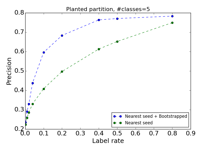
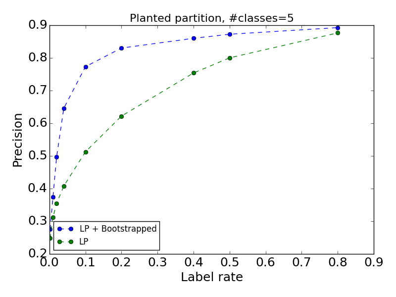
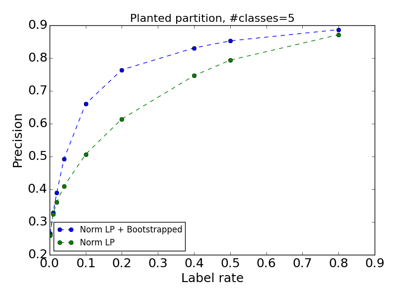
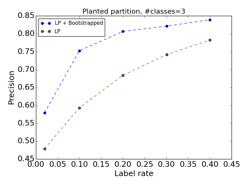
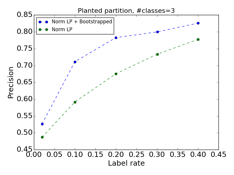
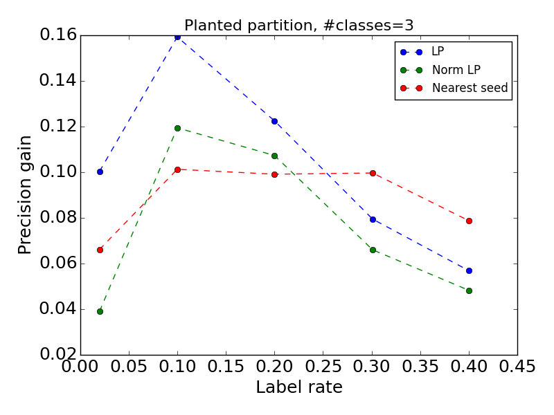
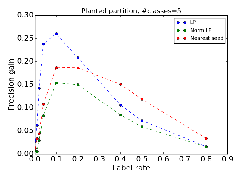
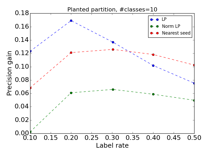
We study the precision of both the base and bootstrapped algorithms as a function of the labeling rate. Here we used $10\times$ random splits of the data sets. For the citation networks and planted partition graphs, we varied the labeling rate while maintaining balanced seed sets that have the same number of seeds from each class. Representative results showing the precision as a function of the labeling rate for selected data sets are visualized in Figure 1. Figure 2 shows the gain in precision due to bootstrapping over the respective base method, as a function of the labeling rate.

The plots show that, as expected, precision of all methods increases with the labeling rate and that bootstrapping consistently improves performance. We can see that across methods, the gain in precision due to bootstrapping is smaller at the extremes, when the labeling rate and precision are very low or very high. The largest gains are obtained in the middle range.

6.2. Seed set augmentations

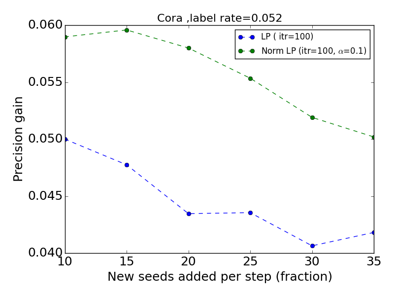
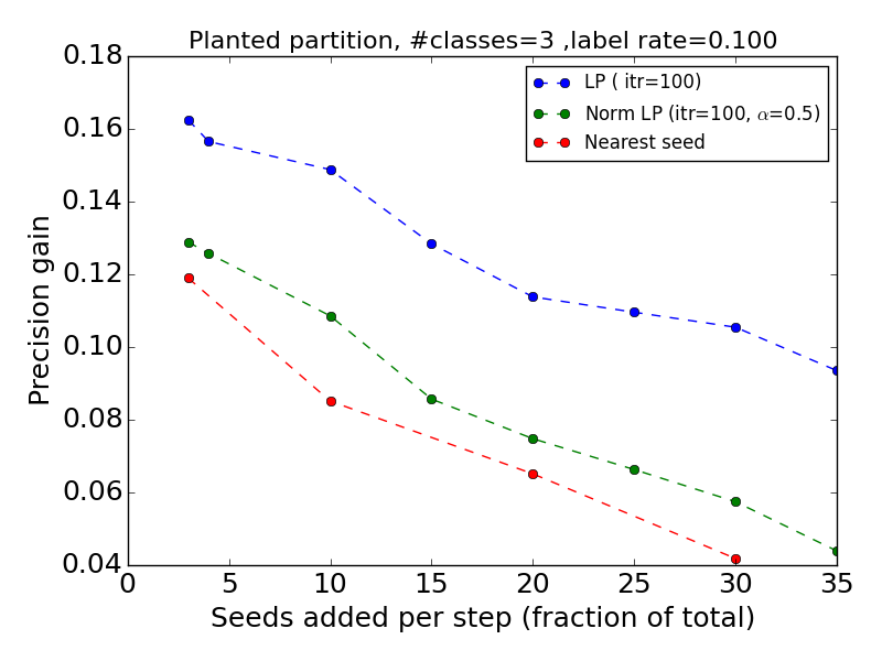
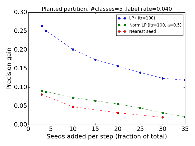
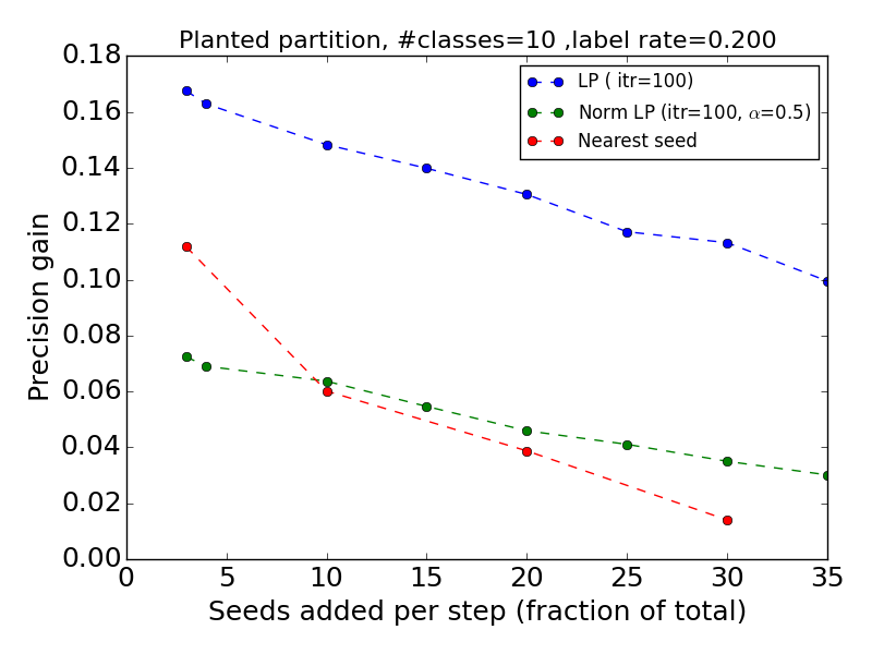
We study the gain in precision as we sweep the bootstrapping parameter $r$, which determines the fraction of nodes that are set as seeds in each bootstrapping step (see Algorithm 4). Figure 3 shows the precision gain as a function of $r$ (in percent) for selected data sets. We can see that as expected the gain decreases with $r$ but that we can obtain significant gains also with relatively large values of $r$.

Figure 3. Precision gain by bootstrapping as a function of the fraction of nodes (in percent) that are set as new seed nodes in each bootstrapping step

6.3. Number of bootstrapping steps

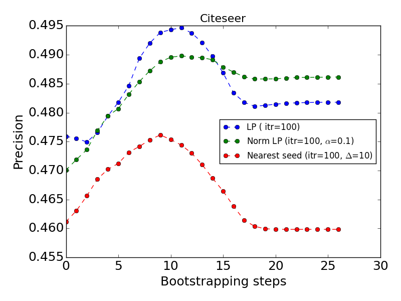
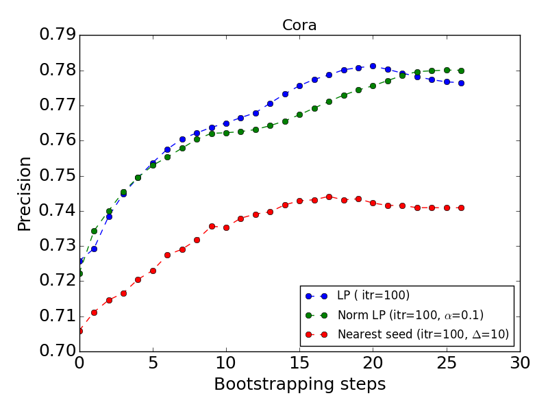
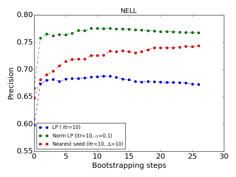
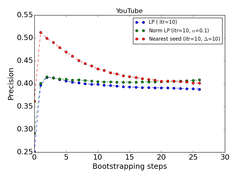
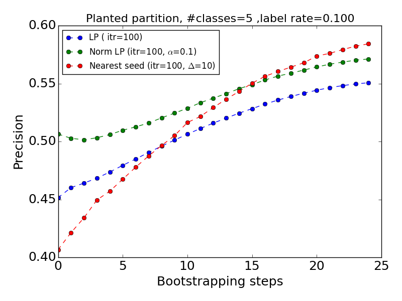
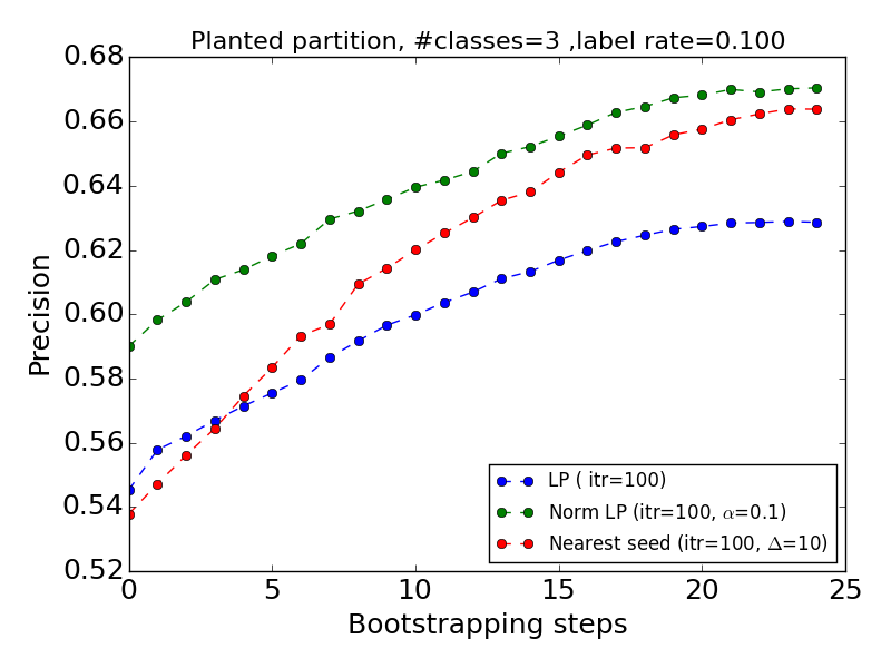
We study the precision as a function of the number of bootstrapping steps performed. In our experiments we used the performance on a validation set to choose the step which provides the final learned labels. Generally, we expect precision to initially improve as the easier-to-predict nodes are added to the seed set and eventually to stabilize or decrease.

Figure 4 shows the precision for each step on representative data sets. In this set of experiments we fixed all other parameters of each algorithm as indicated in the legends of the figure and used a fixed value $r=0.03$ for the fraction of nodes that become new seeds in each step. The results are averaged over 10 random splits of the data. The Figure shows different patterns but all are unimodal which means they allow us to incorporate a stopping criteria for the bootstrapping algorithm.

Figure 4. Precision as a function of the number of steps performed by the bootstrapping wrapper. We used $r=0.03$ and fixed other (hyper)parameters as indicated in the legends.

6.4. Scalability

Optimizing quality is important when labeling is costly. Often, however, on very large graphs, scalability is critical. The computation cost of the methods we considered, social and spectral, bootstrapped or not, depends on the total number of iterations performed.

With label propagation, in each iteration for each node we compute an average over its neighbors. The averaging for different nodes in the same iteration are independent and can be distributed or parallelized. But the iterations sequentially depend on each other. The computation of each iteration involves a linear number of edge traversals and is highly suitable for Pregel-like (pregel:sigmod2010, ) distributed graph processing platforms.

With distance diffusion, each iteration is equivalent to a single-source shortest-paths computation. The number of edge traversals performed is also linear. The iterations here are independent, and can be performed concurrently, each providing independent samples from a distribution. The shortest-path search performed in each iteration, however, has concurrency that depends on the number of hops in the shortest-paths. This computation can also be performed efficiently on Pregel (pregel:sigmod2010, ) by essentially performing all iterations (different sets of hash-specified edge lengths) together. With bootstrapping, the steps must be sequential and in each step we run the base algorithm with multiple iterations.

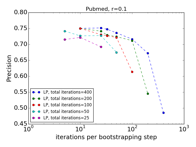
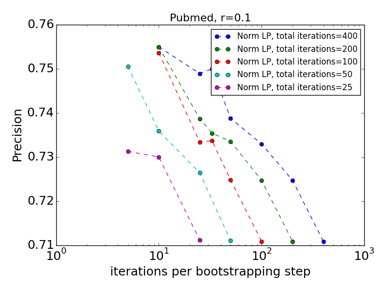
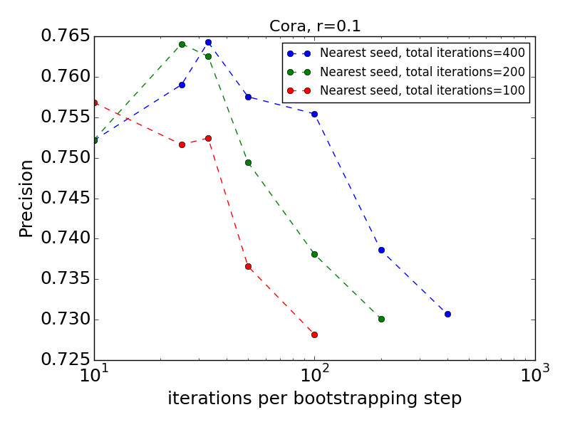
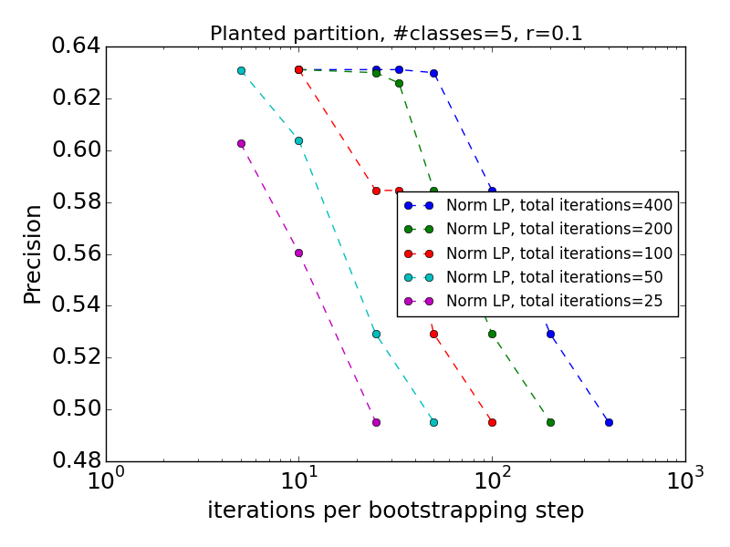
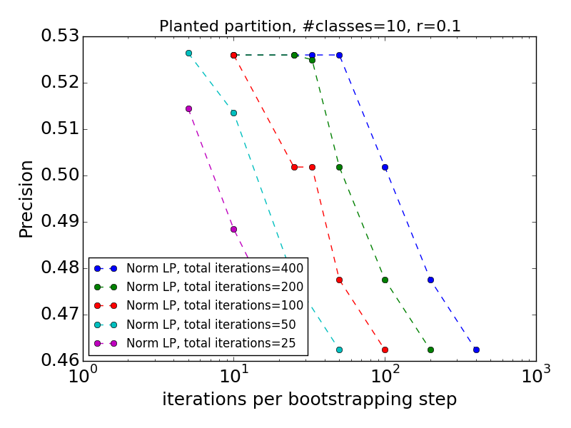
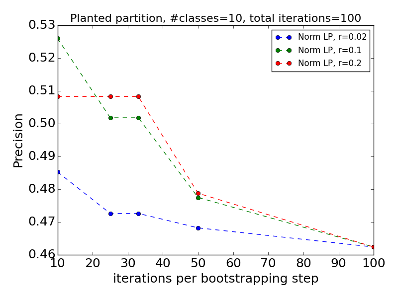
In this set of experiments we study the precision we obtain using a fixed total number of iterations, for different sets of bootstrapping parameters. The plots in Figure 5 show precision as a function of the number of iterations performed in each bootstrapping step. Each graph corresponds to a fixed budget of iterations (between 25 and 400 iterations). The number of iterations performed per step varies between $5$ and the full budget. When all iterations are performed in one step, that is, when the number of iterations per step is equal to the total budget, we have the precision of the non-bootstrapped base algorithm. When we partition the iterations budget to multiple steps we reduce the effectiveness of the base algorithm in each step but can leverage the power of bootstrapping.

Recall that the normalized Laplacian LP and nearest-seed improve with more iterations per step whereas LP may not. We can see that the non-bootstrapped LP algorithm degrades with more iterations (recall that in other experiments we treated the number of iterations with LP it as a hyperparameter). The plot for the Pubmed dataset show that with all budgets, quality picks at 10 iterations per step. With normalized Laplacian LP and nearest-seed (which only improve with iterations), we see that bootstrapped methods with 25 total iterations outperforms the non-bootstrapped algorithms with many more iterations.

Finally, we consider the parameter $r$, which determines the fraction of nodes that are instantiated as new seeds in each step. Generally bootstrapping performance improves with smaller values of the parameter $r$. But with limited iteration budget, and limited number of steps, very low values limit the progress for the bootstrapping. The bottom right plot in Figure 5 shows a sweet spot at $r=0.1$.

Figure 5. Precision for a fixed iteration budget when varying the number of iterations per bootstrapping steps.

7. Feature diffusion

In the previous sections we focused on methods that learn labels using only the graph structure: The provided labels of seed nodes are “diffused” along graph edges to obtain soft labels for all nodes that are then used for prediction. When we have more information, in the form of node feature vectors $\boldsymbol{f}_{i}$ for all nodes $i\leq n_{\ell}+n_{u}$, we can use it for learning. The simplest method, which does not use the graph structure, is to train a supervised classifier on the features and labels of seed nodes $(\tilde{\boldsymbol{f}}_{i},y_{i})$ $i\leq n_{\ell}$. We can instead use the graph structure to obtain diffused feature vectors $\tilde{\boldsymbol{f}}_{i}$. The diffused vectors are a smoothed version of the raw vectors that also reflect features of related nodes, where relation is according to the base diffusion process. Note that the diffused vectors $\tilde{\boldsymbol{f}}_{i}$ do not depend on the set of seed nodes or their labels. A supervised classifier $C$ can then be trained on the diffused features and labels of seed nodes: $(\tilde{\boldsymbol{f}}_{i},y_{i})$ $i\leq n_{\ell}$. When the classifier provides a prediction margin with each classification $C(\tilde{\boldsymbol{f}_{i}})$ for $i>n_{\ell}$, it can be bootstrapped (see algorithm 4).

We evaluated two diffusion methods. Feature Propagation (FP), in Algorithm 5, that uses the diffusion rule of the label propagation method of (ZhuGhahramani2002, ) (Algorithm 1), and Normalized Laplacian FP, in Algorithm 6, that uses the diffusion rule of (ZhouBLWS:NIPS2004, ) (Algorithm 2). We note that our linear feature diffusions can be viewed as a toned-down GCN (AtwoodT:NIPS2016, ; KipfW:ICLR2017, ), without the backprop training, and non-linear aggregations.

Input: Affinity matrix $\boldsymbol{W}$. Node feature vectors $\boldsymbol{f}_{i}$ for $i\leq n_{\ell}+n_{u}$

// Initialize:

$\forall i,\ D_{ii}\leftarrow\sum_{j}W_{ij}$

  // diagonal degree matrix

$\boldsymbol{F}\leftarrow(\boldsymbol{f}_{1},\ldots,\boldsymbol{f}_{n_{\ell}+n_{u}})$

  // Matrix of feature vectors

$\tilde{\boldsymbol{F}}\leftarrow\boldsymbol{F}$

  // Diffused features matrix

// Diffuse:

foreach $t=1,\ldots,T$ do

       $\tilde{\boldsymbol{F}}\leftarrow\boldsymbol{D}^{-1}\boldsymbol{W}\tilde{\boldsymbol{F}}$

      

// Finalize:

return $(\tilde{\boldsymbol{f}}_{1},\ldots,\tilde{\boldsymbol{f}}_{n_{\ell}+n_{u}})\leftarrow\tilde{\boldsymbol{F}}$

  // Diffused feature vectors

Algorithm 5 Feature Propagation (FP)

Input: Affinity matrix $\boldsymbol{W}$. Node feature vectors $\boldsymbol{f}_{i}$ for $i\leq n_{\ell}+n_{u}$. Parameter $\alpha\in(0,1)$

// Initialize:

$\forall i,\ D_{ii}\leftarrow\sum_{j}W_{ij}$

  // diagonal degree matrix

$\boldsymbol{F}\leftarrow(\boldsymbol{f}_{1},\ldots,\boldsymbol{f}_{n_{\ell}+n_{u}})$

  // Matrix of feature vectors

$\tilde{\boldsymbol{F}}\leftarrow\boldsymbol{F}$

  // Diffused features matrix

$\boldsymbol{A}\leftarrow\boldsymbol{D}^{-1/2}\boldsymbol{W}\boldsymbol{D}^{-1/2}$

  // Normalized adjacency matrix

// Diffuse:

foreach $t=0,\ldots,T$ do

       $\tilde{\boldsymbol{F}}\leftarrow(1-\alpha)\boldsymbol{A}\tilde{\boldsymbol{F}}+\alpha\boldsymbol{F}$

return $(\tilde{\boldsymbol{f}}_{1},\ldots,\tilde{\boldsymbol{f}}_{n_{\ell}+n_{u}})\leftarrow\tilde{\boldsymbol{F}}$

  // Diffused feature vectors

Algorithm 6 Normalized Laplacian FP

7.1. Experiments settings

We used the three citation networks dataset (Citeseer, Cora, and Pubmed) listed in Table 1. We use the methodology of Section 3 for the selection of training, test, and validations sets. We use the benchmark fixed seed sets used in prior work (Yang:ICML2016, ; KipfW:ICLR2017, ), to facilitate comparison, and random splits for robustness. The citation networks contain a bag-of-words representation for each document which, following  (Yang:ICML2016, ; KipfW:ICLR2017, ), we treat as a feature vector. The vectors are encoded using 0/1 which indicates the absence/presence of the corresponding term from the dictionary. The dictionaries of Citeseer, Cora and Pubmed contain 3703, 1433 and 500 unique words respectively. For classification from (original and diffused) feature vectors we used one-versus-all logistic regression with the Python sklearn library implementation .

We evaluate the classification quality when using the raw feature vectors $\boldsymbol{f}_{i}$ and when using diffused feature vectors $\tilde{\boldsymbol{f}}_{i}$ obtained using Algorithms 5 and Algorithm 6. For each base algorithm we also apply the bootstrapping wrapper. We used a range of hyper/parameters with a validation set to prevent overfitting: The bootstrapping wrapper was used with $r\in\{0.05,0.1,0.2\}$ as the fraction of new nodes selected as seeds in each step (see Algorithm 4). For FP and normalized Laplacian FP we used $\{2,5,10,20,40,100,200\}$ propagation iterations to compute the diffused feature vectors. For normalized Laplacian FP we used $\alpha\in\{0.01,0.05,0.1,0.2\}$. We comment that the best results across data sets were obtained with $10$ iterations and with $\alpha=0.2$.

7.2. Results on benchmark datasets

Results on benchmark datasets are reported in Table 5. The table also lists for reference the results obtained without using node features by bootstrapped normalized Laplacian LP (experiments in Section 4). For comparison, we also list the quality reported by GCN (KipfW:ICLR2017, ) and Planetoid (Yang:ICML2016, ) (best variant with node features).

We observe the following: First, the quality of learning with diffused feature vectors is significantly better than with the raw feature vectors, with average improvement of about $12\%$. Hence in these data sets the use of the graph structure and the particular way it was used were important. Second, the normalized Laplacian FP was more effective than basic FP. This agrees with our observations with the label propagation experiments. Third, bootstrapping consistently improved performance on two of the data sets (Citeseer and Cora). There was little or no improvement on Pubmed, but on that data sets bootstrapped label propagation (that did not used the node features) was the near-best performer. Fourth, the bootstrapped version of normalized Laplacian FP improves over the state of the art results of GCN (KipfW:ICLR2017, ) on Citeseer and Cora. On Pubmed GCN was only slightly better than our bootstrapped label propagation.

7.3. Results on random splits

In this set of experiments, for each data set, we generated multiple random splits of the nodes to seed, test, and validation sets and averaged the results. Our results are reported in Table 6. For reference, we also list the results using label propagation (without the use of node features) that we reported in Section 5 and the results reported on similar random splits using GCNs (KipfW:ICLR2017, ). The results add robustness to our observations from the benchmark experiments: The use of diffused features significantly improves quality, the normalized Laplacian FP consistently achieves the best results on Citeseer and Cora and is very close (within error margins) to the results reported by (KipfW:ICLR2017, ) on Pubmed.

Table 5. Feature diffusion results for benchmark data

Method	Citeseer	Cora	Pubmed
Norm Lap LP(ZhouBLWS:NIPS2004, ) +Bootstrapped	0.536	0.784	0.788
no feature diffusion	0.604	0.589	0.729
+Bootstrapped	0.683	0.655	0.729
Feature propagation	0.687	0.804	0.779
+Bootstrapped	0.703	0.798	0.711
Norm feature propagation	0.696	0.824	0.765
+Bootstrapped	0.728	0.829	0.765
Graph Conv Nets (KipfW:ICLR2017, )	0.703	0.815	0.790
Planetoid (Yang:ICML2016, )	0.629	0.757	0.757

Table 6. Feature diffusion results over random splits

Method	Citeseer	Cora	Pubmed
$\times$ repetitions	100	100	100
Label Propagation(ZhuGhahramani2002, )	0.479	0.728	0.709
+Bootstrapped	0.496	0.781	0.747
Norm Lap LP (ZhouBLWS:NIPS2004, )	0.490	0.730	0.739
+Bootstrapped	0.503	0.782	0.756
$\times$ repetitions	10	10	10
no feature diffusion	0.614	0.608	0.719
+Bootstrapped	0.695	0.695	0.757
Feature propagation	0.703	0.808	0.781
+Bootstrapped	0.719	0.832	0.781
Norm feature propagation	0.727	0.831	0.785
+Bootstrapped	0.737	0.848	0.785
Graph Conv Nets (KipfW:ICLR2017, )	0.679	0.801	0.789

8. Conclusion

We studied the application of self-training, which is perhaps the most basic form of introducing non-linearity, to SSL methods based on linear graph diffusions. We observed that the resulting bootstrapped diffusions ubiquitously improved labeling quality over the respective base methods on a variety of real-world and synthetic data sets. Moreover, we obtain state-of-the-art quality, previously achieved by more complex methods, while retaining the high scalability of the base methods.

Our results are a proof of concept that uses the simplest base algorithms and bootstrapping wrapper. Some natural extensions include fine tuning of the wrapper together with base algorithms that provide more precise confidence scores and the use of a richer set of base algorithms.

On a final note, we recall that spectral and social graph diffusions are an important tool in graph mining: They are the basis of centrality, influence, and similarity measures of a node or sets of nodes in a network (Chung:Book97a, ; pagerank:1999, ; KKT:KDD2003, ; BlochJackson:2007, ; CoKa:jcss07, ; Opsahl:2010, ; GRLK:KDD2010, ; CDFGGW:COSN2013, ; DSGZ:nips2013, ; timedinfluence:2015, ) and also underline community detection and local clustering algorithms (SpielmanTeng:sicomp2013, ). Our work suggests that substantial gains in quality might be possible by using bootstrapped diffusions as an alternative to classic ones in these wider contexts. We hope to pursue this in future work.