Synchronization of phase oscillators
on the hierarchical lattice

Abstract

Synchronization of neurons forming a network with a hierarchical structure is essential for the brain to be able to function optimally. In this paper we study synchronization of phase oscillators on the most basic example of such a network, namely, the hierarchical lattice. Each site of the lattice carries an oscillator that is subject to noise. Pairs of oscillators interact with each other at a strength that depends on their hierarchical distance, modulated by a sequence of interaction parameters. We look at block averages of the oscillators on successive hierarchical scales, which we think of as block communities. In the limit as the number of oscillators per community tends to infinity, referred to as the hierarchical mean-field limit, we find a separation of time scales, i.e., each block community behaves like a single oscillator evolving on its own time scale. We argue that the evolution of the block communities is given by a renormalized mean-field noisy Kuramoto equation, with a synchronization level that depends on the hierarchical scale of the block community. We find three universality classes for the synchronization levels on successive hierarchical scales, characterized in terms of the sequence of interaction parameters.

What makes our model specifically challenging is the non-linearity of the interaction between the oscillators. The main results of our paper therefore come in three parts: (I) a conjecture about the nature of the renormalisation transformation connecting successive hierarchical scales; (II) a truncation approximation that leads to a simplified renormalization transformation; (III) a rigorous analysis of the simplified renormalization transformation. We provide compelling arguments in support of (I) and (II), but a full verification remains an open problem.

Mathematics Subject Classification 2010. 60K35, 60K37, 82B20, 82C27, 82C28.

Key words and phrases. Hierarchical lattice, phase oscillators, noisy Kuramoto model, block communities, renormalization, universality classes.

Acknowledgment. DG is supported by EU-project 317532-MULTIPLEX. FdH and JM are supported by NWO Gravitation Grant 024.002.003–NETWORKS. The authors are grateful to G. Giacomin for critical remarks.

1 Introduction

The concept of spontaneous synchronization is ubiquitous in nature. Single oscillators (like flashing fireflies, chirping crickets or spiking brain cells) may rotate incoherently, at their own natural frequency, when they are isolated from the population, but within the population they adapt their rhythm to that of the other oscillators, acting as a system of coupled oscillators. There is no central driving mechanism, yet the population reaches a globally synchronized state via mutual local interactions.

The omnipresence of spontaneous synchronization triggered scientists to search for a mathematical approach in order to understand the underlying principles. The first steps were taken by Winfree [19], [20], who recognized that spontaneous synchronization should be understood as a threshold phenomenon: if the coupling between the oscillators is sufficiently strong, then a macroscopic part of the population freezes into synchrony. Although the model proposed by Winfree was too difficult to solve analytically, it inspired Kuramoto  [8], [9] to suggest a more mathematically tractable model that captures the same phenomenon. The Kuramoto model has since been used successfully to study synchronization in a variety of different contexts. By now there is an extended literature, covering aspects like phase transition, stability, and effect of disorder (for a review, see Acébron et al. [1]).

Mathematically, the Kuramoto model still poses many challenges. As long as the interaction is mean-field (meaning that every oscillator interacts equally strongly with every other oscillator), a fairly complete theory has been developed. However, as soon as the interaction has a non-trivial geometry, computations become cumbersome. There is a large literature for the Kuramoto model on complex networks, where the population is viewed as a random graph whose vertices carry the oscillators and whose edges represent the interaction. Numerical and heuristic results have been obtained for networks with a small-world, scale-free and/or community structure, showing a range of interesting phenomena (for a review, see Arenas et al. [2]). Rigorous results are rare. In the present paper we focus on one particular network with a community structure, namely, the hierarchical lattice.

The remainder of this paper is organised as follows. Sections 1.1–1.3 are devoted to the mean-field noisy Kuramoto model. In Section 1.1 we recall definitions and basic properties. In Section 1.2 we recall the McKean-Vlasov equation, which describes the evolution of the probability density for the phase oscillators in the mean-field limit. In Section 1.3 we take a closer look at the scaling properties of the order parameters towards the mean-field limit. In Section 1.4 we define the hierarchical lattice and in Section 1.5 introduce the noisy Kuramoto model on the hierarchical lattice, which involves a sequence of interaction strengths $(K_{k})_{k\in\mathbb{N}}$ acting on successive hierarchical levels. Section 2 contains our main results, presented in the form of a conjecture, a truncation approximation, and rigrorous theorems. These concern the hierarchical mean-field limit and show that, for each $k\in\mathbb{N}$, the block communities at hierarchical level $k$ behave like the mean-field noisy Kuramoto model, with an interaction strength and a noise that depend on $k$ and are obtained via a renormalization transformation connecting successive hierarchical levels. There are three universality classes for $(K_{k})_{k\in\mathbb{N}}$, corresponding to sudden loss of synchronization at a finite hierarchical level, gradual loss of synchronization as the hierarchical level tends to infinity, and no loss of synchronization. The renormalization transformation allows us to describe these classes in some detail. In Section 3 we analyse the renormalization scheme, in Section 4 we find criteria for the universality classes. Appendix A provides numerical examples and computations.

1.1 Mean-field Kuramoto model

We begin by reviewing the mean-field Kuramoto model. Consider a population of $N\in\mathbb{N}$ oscillators, and suppose that the $i^{\text{th}}$ oscillator has a natural frequency $\omega_{i}$, such that

$$\blacktriangleright \omega_{i},\,i=1,\ldots,N,\text{ are i.i.d.\ and are drawn from}$$ (1.1)

$$\text{a common probability distribution }\mu\text{ on }\mathbb{R}.$$

Let the phase of the $i^{\text{th}}$ oscillator at time $t$ be $\theta_{i}(t)\in\mathbb{R}$. If the oscillators were not interacting, then we would have the system of uncoupled differential equations

$$\frac{\mathrm{d}\theta_{i}(t)}{\mathrm{d}t}=\omega_{i},\quad i=1,\ldots,N.$$ (1.2)

Kuramoto [8], [9] realized that the easiest way to allow for synchronization was to let every oscillator interact with every other oscillator according to the sine of their phase difference, i.e., to replace (1.2) by:

$$\frac{\mathrm{d}\theta_{i}(t)}{\mathrm{d}t}=\omega_{i}+\frac{K}{N}\sum_{j=1}^{N}\sin\big{[}\theta_{j}(t)-\theta_{i}(t)\big{]},\quad i=1,\ldots,N.$$ (1.3)

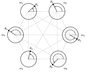
Here, $K\in(0,\infty)$ is the interaction strength, and the factor $\frac{1}{N}$ is included to make sure that the total interaction per oscillator stays finite in the thermodynamic limit $N\to\infty$. The coupled evolution equations in (1.3) are referred to as the mean-field Kuramoto model. An illustration of the interaction in this model is given in Fig. 1.

Figure 1: Mean-field interaction of $N=6$ oscillators with natural frequencies $\omega_{i}$ and phases $\theta_{i}$, $i=1,\ldots,6$, evolving according to (1.3).

If noise is added, then (1.3) turns into the mean-field noisy Kuramoto model, given by

$$\mathrm{d}\theta_{i}(t)=\omega_{i}\,\mathrm{d}t+\frac{K}{N}\sum_{j=1}^{N}\sin\big{[}\theta_{j}(t)-\theta_{i}(t)\big{]}\,\mathrm{d}t+D\,\mathrm{d}W_{i}(t),\quad i=1,\ldots,N.$$ (1.4)

Here, $D\in(0,\infty)$ is the noise strength, and $(W_{i}(t))_{t\geq 0}$, $i=1,\ldots,N$, are independent standard Brownian motions on $\mathbb{R}$. The coupled evolution equations in (1.4) are stochastic differential equations in the sense of Itô (see e.g. Karatzas and Shreve [7]). As initial condition we take

$$\blacktriangleright \theta_{i}(0),\,i=1,\ldots,N,\text{ are i.i.d.\ and are drawn from}$$ (1.5)

$$\text{a common probability distribution }\rho\text{ on }[0,2\pi).$$

In order to exploit the mean-field nature of (1.4), the complex-valued order parameter (with $\mathrm{i}$ the imaginary unit)

$$r_{N}(t)\,\mathrm{e}^{\mathrm{i}\psi_{N}(t)}=\frac{1}{N}\sum_{j=1}^{N}\mathrm{e}^{\mathrm{i}\theta_{j}(t)}$$ (1.6)

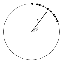
is introduced. In (1.6), $r_{N}(t)$ is the synchronization level at time $t$ and takes values in $[0,1]$, while $\psi_{N}(t)$ is the average phase at time $t$ and takes values in $[0,2\pi)$. (Note that $\psi_{N}(t)$ is properly defined only when $r_{N}(t)>0$.) The order parameter $(r,\psi)$ is illustrated in Fig. 2 ($r=0$ corresponds to the oscillators being completely unsynchronized, $r=1$ to the oscillators being completely synchronized).

(a) $r=0.095$.

(b) $r=0.929$.

Figure 2: Phase distribution of oscillators for two different values of $r$. The arrow represents the complex number $r\mathrm{e}^{i\psi}$.

By rewriting (1.4) in terms of (1.6) as

$$\mathrm{d}\theta_{i}(t)=\omega_{i}\,\mathrm{d}t+Kr_{N}(t)\sin\big{[}\psi_{N}(t)-\theta_{i}(t)\big{]}\,\mathrm{d}t+D\,\mathrm{d}W_{i}(t),\quad i=1,\ldots,N,$$ (1.7)

we see that the oscillators are coupled via the order parameter, i.e., the phases $\theta_{i}$ are pulled towards $\psi_{N}$ with a strength proportional to $r_{N}$. Note that $r_{N}(t)$ and $\psi_{N}(t)$ are random variables that depend on $\mu$, $D$ and $\rho$.

In the mean-field limit $N\to\infty$, the system in (1.7) exhibits what is called “propagation of chaos”, i.e., the evolution of single oscillators becomes autonomous. Indeed, let the order parameter associated with $\rho$ in (1.5) be the pair $(R,\Phi)\in[0,1]\times[0,2\pi)$ defined by

$$R\,\mathrm{e}^{\mathrm{i}\Phi}=\int_{0}^{2\pi}\rho(\mathrm{d}\theta)\,\mathrm{e}^{\mathrm{i}\theta}.$$ (1.8)

Suppose that $R>0$, so that $\Phi$ is properly defined. Suppose further that

$$\blacktriangleright\quad\text{the disorder distribution }\mu\text{ in \eqref{eq:frequencies} is symmetric}.$$ (1.9)

Then, as we will see in Sections 1.2–1.3, the limit as $N\to\infty$ of the evolution of a single oscillator, say $\theta_{1}$, is given by

$$\mathrm{d}\theta_{1}(t)=\omega_{1}\,\mathrm{d}t+Kr(t)\sin\big{[}\Phi-\theta_{1}(t)\big{]}\,\mathrm{d}t+D\,\mathrm{d}W_{1}(t),$$ (1.10)

where $(W_{1}(t))_{t\geq 0}$ is a standard Brownian motion, and $r(t)$ is driven by a deterministic relaxation equation such that

$$r(0)=R,\qquad\lim_{t\to\infty}r(t)=r\text{ for some }r\in[0,1).$$ (1.11)

The parameter $r=r(\mu,D,K)$ will be identified in (1.21) below (and the convergence holds at least when $R$ is close to $r$; see Remark 1.1 below). The evolution in (1.10) is not closed because of the presence of $r(t)$, but after a transient period it converges to the autonomous evolution equation

$$\mathrm{d}\theta_{1}(t)=\omega_{1}\,\mathrm{d}t+Kr\sin\big{[}\Phi-\theta_{1}(t)\big{]}\,\mathrm{d}t+D\,\mathrm{d}W_{1}(t).$$ (1.12)

Without loss of generality, we may calibrate $\Phi=0$ by rotating the circle $[0,2\pi)$ over $-\Phi$. After that the parameters $R,\Phi$ associated the initial distribution $\rho$ are gone, and only $r$ remains as the relevant parameter. It is known (see e.g. (1.23) below) that there exists a critical threshold $K_{c}=K(\mu,D)\in(0,\infty)$ separating two regimes:

• For $K\in(0,K_{c}]$ the system relaxes to an unsynchronized state ($r=0$).

• For $K\in(K_{c},\infty)$ the system relaxes to a partially synchronized state ($r\in(0,1)$), at least when $\rho$ in (1.5) is chosen such that $R$ is close to $r$ (see Remark 1.1 below).

See Strogatz [16] and Luçon [11] for overviews.

1.2 McKean-Vlasov equation

For the system in (1.4), Sakaguchi [13] showed that in the limit as $N\to\infty$, the probability density for the phase oscillators and their natural frequencies (with respect to $\lambda\times\mu$, with $\lambda$ the Lebesgue measure on $[0,2\pi]$ and $\mu$ the disorder measure on $\mathbb{R}$) evolves according to the McKean-Vlasov equation

$$\frac{\partial}{\partial t}\,p(t;\theta,\omega)=-\frac{\partial}{\partial\theta}\,\Big{[}p(t;\theta,\omega)\,\Big{\{}\omega+Kr(t)\sin\big{[}\psi(t)-\theta\big{]}\Big{\}}\Big{]}+\frac{D}{2}\frac{\partial^{2}}{\partial\theta^{2}}\,p(t;\theta,\omega),$$ (1.13)

where

$$r(t)\,\mathrm{e}^{\mathrm{i}\psi(t)}=\int_{\mathbb{R}}\mu(\mathrm{d}\omega)\int_{0}^{2\pi}\mathrm{d}\theta\,\mathrm{e}^{\mathrm{i}\theta}\,p(t;\theta,\omega),$$ (1.14)

is the continuous counterpart of (1.6). If $\rho$ has a density, say $\rho(\theta)$, then $p(0;\theta,\omega)=\rho(\theta)$ for all $\omega\in\mathbb{R}$.

By (1.9), we can again calibrate the average phase to be zero, i.e., $\psi(t)=\psi(0)=\Phi=0$, $t\geq 0$, in which case the stationary solutions of (1.13) satisfy

$$0=-\frac{\partial}{\partial\theta}\,\big{[}p(\theta,\omega)\,(\omega-Kr\sin\theta)\big{]}+\frac{D}{2}\frac{\partial^{2}}{\partial\theta^{2}}\,p(\theta,\omega).$$ (1.15)

The solutions of (1.15) are of the form

$$p_{\lambda}(\theta,\omega)=\frac{A_{\lambda}(\theta,\omega)}{\int_{0}^{2\pi}\mathrm{d}\phi\,A_{\lambda}(\phi,\omega)},\qquad\lambda=2Kr/D,$$ (1.16)

with

$$A_{\lambda}(\theta,\omega) =B_{\lambda}(\theta,\omega)\left(\mathrm{e}^{4\pi\omega}\int_{0}^{2\pi}\frac{\mathrm{d}\phi}{B_{\lambda}(\phi,\omega)}+(1-\mathrm{e}^{4\pi\omega})\int_{0}^{\theta}\frac{\mathrm{d}\phi}{B_{\lambda}(\phi,\omega)}\right),$$ (1.17)

$$B_{\lambda}(\theta,\omega) =\mathrm{e}^{\lambda\cos\theta+2\theta\omega}.$$

After rewriting

$$A_{\lambda}(\theta,\omega)=B_{\lambda}(\theta,\omega)\left(\int_{\theta-2\pi}^{0}\frac{\mathrm{d}\phi}{B_{\lambda}(-\phi,-\omega)}+\int_{0}^{\theta}\frac{\mathrm{d}\phi}{B_{\lambda}(\phi,\omega)}\right)$$ (1.18)

and noting that $B_{\lambda}(\phi,\omega)=B_{\lambda}(-\phi,-\omega)$, we easily check that

$$p_{\lambda}(\theta,\omega)=p_{\lambda}(-\theta,-\omega),$$ (1.19)

a property we will need later. In particular, in view of (1.9), we have

$$\int_{\mathbb{R}}\mu(\mathrm{d}\omega)\int_{0}^{2\pi}\mathrm{d}\theta\,p_{\lambda}(\theta,\omega)\,\sin\theta=0.$$ (1.20)

Since $\psi(t)=\psi(0)=\Phi=0$, we see from (1.14) that $p_{\lambda}(\theta,\omega)$ in (1.16) is a solution if and only if $r$ satisfies

$$\int_{\mathbb{R}}\mu(\mathrm{d}\omega)\int_{0}^{2\pi}\mathrm{d}\theta\,p_{\lambda}(\theta,\omega)\,\cos\theta=r,\qquad\lambda=2Kr/D.$$ (1.21)

This gives us a self-consistency relation for

$$r=r(D,K)$$ (1.22)

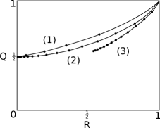
a situation that is typical for mean-field systems, which can in principle be solved (and possibly has more than one solution). The equation in (1.21) always has a solution with $r=0$: the unsynchronized state corresponding to $p_{0}(\theta,\omega)=\frac{1}{2\pi}$ for all $\theta,\omega$. A (not necessarily unique) solution with $r\in(0,1)$ exists when the coupling strength $K$ exceeds a critical threshold $K_{c}=K_{c}(\mu,D)$. When this occurs, we say that the oscillators are in a partially synchronized state. As $K$ increases also $r$ increases (see Fig. 3). Moreover, $r\uparrow 1$ as $K\to\infty$ and we say that the oscillators converge to a fully synchronized state. When $K$ crosses $K_{c}$, the system exhibits a second-order phase transition, i.e., $K\mapsto r(K)$ is continuous at $K=K_{c}$.

Figure 3: Picture of $K\mapsto r(K)$ for fixed $\mu$ and $D$.

For the case where the frequency distribution $\mu$ is symmetric and unimodal, an explicit expression is known for $K_{c}$:

$$\frac{1}{K_{c}}=\int_{\mathbb{R}}\mu(\mathrm{d}\omega)\,\frac{D}{D^{2}+4\omega^{2}}.$$ (1.23)

Thus, when the spread of $\mu$ is large compared to $K$, the oscillators are not able to synchronize and they rotate near their own frequencies. As $K$ increases, this remains the case until $K$ reaches $K_{c}$. After that a small fraction of synchronized oscillators starts to emerge, which becomes of macroscopic size when $K$ moves beyond $K_{c}$. For $\mu$ symmetric and unimodal it is conjectured that for $K>K_{c}$ there is a unique synchronized solution $p_{\lambda}(\cdot,\cdot)$ with $r\in(0,1)$ solving (1.21) (Luçon [11, Conjecture 3.12]). This conjecture has been proved when $\mu$ is narrow, i.e., the disorder is small (Luçon [11, Proposition 3.13]).

Remark 1.1.

Stability of stationary solutions has been studied by Strogatz and Mirollo [17], Strogatz, Mirollo and Matthews [18], Luçon [11, Section 3.4]. For symmetric unimodal disorder, the unsynchronized state is linearly stable for $K<K_{c}$ and linearly unstable for $K>K_{c}$, while the synchronized state for $K>K_{c}$ is linearly stable at least for small disorder. Not much is known about stability for general disorder. ∎

There is no closed form expression for $K_{c}$ beyond symmetric unimodal disorder, except for special cases, e.g. symmetric binary disorder. We refer to Luçon [11] for an overview. A large deviation analysis of the empirical process of oscillators has been carried out in Dai Pra and den Hollander [5].

1.3 Diffusive scaling of the average phase

Bertini, Giacomin and Poquet [3] showed that for the mean-field noisy Kuramoto model without disorder, in the limit as $N\to\infty$ the synchronization level evolves on time scale $t$ and converges to a deterministic limit, while the average phase evolves on time scale $Nt$ and converges to a Brownian motion with a renormalized noise strength.

Theorem 1.2 (Bertini, Giacomin and Poquet [3]).

Suppose that $\mu=\delta_{0}$ and $r>0$. Then, in distribution,

$$\lim_{N\to\infty}\psi_{N}(Nt)=\psi_{*}(t),$$ (1.24)

$$\lim_{N\to\infty}r_{N}(t)=r(t),$$

with

$$\begin{array}[]{lll}&\mathrm{d}\psi_{*}(t)=D_{*}\,\mathrm{d}W_{*}(t),&\psi_{*}(0)=\Phi,\\ &\lim_{t\to\infty}r(t)=r,&r(0)=R,\end{array}$$ (1.25)

where $(W_{*}(t))_{t\geq 0}$ is a standard Brownian motion and

$$D_{*}=D_{*}(D,K,r)=\frac{1}{\sqrt{1-[I_{0}(2Kr/D)]^{-2}}},\qquad r=r(D,K),$$ (1.26)

with $I_{0}$ the modified Bessel function of order zero given by

$$I_{0}(\lambda)=\frac{1}{2\pi}\int_{0}^{2\pi}\mathrm{d}\theta\,\mathrm{e}^{\lambda\cos\theta},\qquad\lambda\in[0,\infty).$$ (1.27)

The work in [3] also shows that

$$\lim_{N\to\infty}r_{N}(Nt)=r\qquad\forall\,t>0,$$ (1.28)

i.e., the synchronization level not only tends to $r$ over time, it also stays close to $r$ on a time scale of order $N$. Thus, the synchronization level is much less volatile than the average phase.

In Section 3.1 we explain the heuristics behind Theorem 1.2. This heuristics will play a key role in our analysis of the Kuramoto model on the hierarchical lattice in the hierarchical mean-field limit. In fact, Conjecture 2.1 below will extend Theorem 1.2 to the hierarchical lattice. It is important to note that the diffusive scaling only occurs in the model without disorder. Indeed, for the model with disorder it was shown in Luçon and Poquet [12] that the fluctuations of the disorder prevail over the fluctuations of the noise, resulting in ‘travelling waves’ for the empirical distribution of the oscillators. Therefore, also on the hierarchical lattice we only consider the model without disorder.

1.4 Hierarchical lattice

The hierarchical lattice of order $N$ consist of countable many vertices that form communities of sizes $N$, $N^{2}$, etc. For example, the hierarchical lattice of order $N=3$ consists of vertices that are grouped into $1$-block communities of $3$ vertices, which in turn are grouped into $2$-block communities of $9$ vertices, and so on. Each vertex is assigned a label that defines its location at each block level (see Fig. 4).

Figure 4: The hierarchical lattice of order $N=3$. The vertices live at the lowest level. The tree visualizes their distance: the distance between two vertices $\eta,\zeta$ is the height of their lowest common branching point in the tree: $d(\eta,\zeta)=2$ in the picture.

Formally, the hierarchical group $\Omega_{N}$ of order $N\in\mathbb{N}\backslash\{1\}$ is the set

$$\Omega_{N}=\bigg{\{}\eta=(\eta^{\ell})_{\ell\in\mathbb{N}_{0}}\in\{0,1,\ldots,N-1\}^{\mathbb{N}_{0}}\colon\,\sum_{\ell\in\mathbb{N}_{0}}\eta^{\ell}<\infty\bigg{\}}$$ (1.29)

with addition modulo $N$, i.e., $(\eta+\zeta)^{\ell}=\eta^{\ell}+\zeta^{\ell}\,(\text{mod}\,N)$, $\ell\in\mathbb{N}_{0}$. The distance on $\Omega_{N}$ is defined as

$$d\colon\,\Omega_{N}\times\Omega_{N}\to\mathbb{N}_{0},\quad(\eta,\zeta)\mapsto\min\big{\{}k\in\mathbb{N}_{0}\colon\,\eta^{\ell}=\zeta^{\ell}\,\,\forall\,\ell\geq k\big{\}},$$ (1.30)

i.e., the distance between two vertices is the smallest index from which onwards the sequences of hierarchical labels of the two vertices agree. This distance is ultrametric:

$$d(\eta,\zeta)\leq\min\{d(\eta,\xi),d(\zeta,\xi)\}\qquad\forall\,\eta,\zeta,\xi\in\Omega_{N}.$$ (1.31)

For $\eta\in\Omega_{N}$ and $k\in\mathbb{N}_{0}$, the $k$-block around $\eta$ is defined as

$$B_{k}(\eta)=\{\zeta\in\Omega_{N}\colon\,d(\eta,\zeta)\leq k\}.$$ (1.32)

1.5 Hierarchical Kuramoto model

We are now ready to define the model that will be our object of study. Each vertex $\eta\in\Omega_{N}$ carries a phase oscillator, whose phase at time $t$ is denoted by $\theta_{\eta}(t)$. Oscillators interact in pairs, but at a strength that depends on their hierarchical distance. To modulate this interaction, we introduce a sequence of interaction strengths

$$(K_{k})_{k\in\mathbb{N}}\in(0,\infty)^{\mathbb{N}},$$ (1.33)

and we let each pair of oscillators $\eta,\zeta\in\Omega_{N}$ at distance $d(\eta,\zeta)=d$ interact as in the mean-field Kuramoto model with $K/N$ replaced by $K_{d}/N^{2d-1}$, where the scaling factor is chosen to ensure that the model remains well behaved in the limit as $N\to\infty$. Thus, our coupled evolution equations read

$$\mathrm{d}\theta_{\eta}(t)=\sum_{\zeta\in\Omega_{N}}\frac{K_{d(\eta,\zeta)}}{N^{2d(\eta,\zeta)-1}}\,\sin\big{[}\theta_{\zeta}(t)-\theta_{\eta}(t)\big{]}\,\mathrm{d}t+D\,\mathrm{d}W_{\eta}(t),\qquad\eta\in\Omega_{N},t\geq 0,$$ (1.34)

where $(W_{\eta}(t))_{t\geq 0}$, $\eta\in\Omega_{N}$, are i.i.d. standard Brownian motions. As initial condition we take, as in (1.5),

$$\blacktriangleright \theta_{\eta}(0),\,\eta\in\Omega_{N},\text{ are i.i.d.\ and are drawn from}$$ (1.35)

$$\text{a common probability distribution }\rho(\mathrm{d}\theta)\text{ on }[0,2\pi).$$

We will be interested in understanding the evolution of average phase in the definition of the order parameter associated with the $N^{k}$ oscillators in the $k$-block around $\eta$ at time $N^{k}t$, defined by

$$R_{\eta,N}^{[k]}(Nt)\,\mathrm{e}^{\mathrm{i}\Phi_{\eta,N}^{[k]}(t)}=\frac{1}{N^{k}}\sum_{\zeta\in B_{k}(\eta)}\mathrm{e}^{\mathrm{i}\theta_{\zeta}(N^{k}t)},\qquad\eta\in\Omega_{N},t\geq 0,$$ (1.36)

where $R_{\eta,N}^{[k]}(Nt)$ is the synchronization level at time $N^{k}t$ and $\Phi_{\eta,N}^{[k]}(t)$ is the average phase at time $N^{k}t$. The new time scales $Nt$ and $t$ will turn out to be natural in view of the scaling in Theorem 1.2. The synchronization level $R_{\eta,N}^{[k]}$ captures the synchronization of the $(k-1)$-blocks, of which there are $N$ in total constituting the $k$-block around $\eta$. These blocks must synchronize before their average phase $\Phi_{\eta,N}^{[k]}$ can begin to move, which is why $R_{\eta,N}^{[k]}$ moves on a different time scale compared to $\Phi_{\eta,N}^{[k]}$. Our goal will be to pass to the limit $N\to\infty$, look at the limiting synchronization levels around a given vertex, say $\eta=0^{\mathbb{N}}$, and classify the scaling behavior of these synchronization levels as $k\to\infty$ into universality classes according to the choice of $(K_{k})_{k\in\mathbb{N}}$ in (1.33).

Note that, for every $\eta\in\Omega_{N}$, we can telescope to write

$$\sum_{\zeta\in\Omega_{N}}\frac{K_{d(\zeta,\eta)}}{N^{2d(\eta,\zeta)-1}}\sin\big{[}\theta_{\zeta}(t)-\theta_{\eta}(t)\big{]} =\sum_{k\in\mathbb{N}}\frac{K_{k}}{N^{2k-1}}\sum_{\zeta\in B_{k}(\eta)/B_{k-1}(\eta)}\sin\big{[}\theta_{\zeta}(t)-\theta_{\eta}(t)\big{]}$$ (1.37)

$$=\sum_{k\in\mathbb{N}}\Big{(}\frac{K_{k}}{N^{2k-1}}-\frac{K_{k+1}}{N^{2(k+1)-1}}\Big{)}\sum_{\zeta\in B_{k}(\eta)}\sin\big{[}\theta_{\zeta}(t)-\theta_{\eta}(t)\big{]}.$$

Inserting (1.37) into (1.34) and using (1.36), we get

$$\mathrm{d}\theta_{\eta}(t)$$ (1.38)

$$\qquad=\sum_{k\in\mathbb{N}}\frac{1}{N^{k-1}}\Big{(}K_{k}-\frac{K_{k+1}}{N^{2}}\Big{)}\,R_{\eta,N}^{[k]}(N^{1-k}t)\,\sin\Big{[}\Phi_{\eta,N}^{[k]}(N^{-k}t)-\theta_{\eta}(t)\Big{]}\,\mathrm{d}t+D\,\mathrm{d}W_{\eta}(t).$$

This shows that, like in (1.7), the oscillators are coupled via the order parameters associated with the $k$-blocks for all $k\in\mathbb{N}$, suitably weighted. As for the mean-field Kuramoto model, for every $\eta\in\Omega_{N}$, $R_{\eta,N}^{[k]}(N^{1-k}t)$ and $\Phi_{\eta,N}^{[k]}(N^{-k}t)$ are random variables that depend on $(K_{k})_{k\in\mathbb{N}}$ and $D$.

When we pass to the limit $N\to\infty$ in (1.38), in the right-hand side of (1.38) only the term with $k=1$ survives, so that we end up with an autonomous evolution equation similar to (1.10). The goal of the present paper is to show that a similar decoupling occurs at all block levels. Indeed, we expect the successive time scales at which synchronization occurs to separate. If there is synchronization at scale $k$, then we expect the average of the $k$-blocks around the origin forming the $(k+1)$-blocks (of which there are $N$ in total) to behave as if they were single oscillators at scale $k+1$.

Dahms [4] considers a multi-layer model with a different type of interaction: single layers labelled by $\mathbb{N}$, each consisting of $N$ oscillators, are stacked on top of each other, and each oscillator in each layer is interacting with the average phases of the oscillators in all the other layers, with interaction strengths $(\tilde{K}_{k})_{k\in\mathbb{N}}$ (see [4, Section 1.3]). For this model a necessary and sufficient criterion is derived for synchronization to be present at all levels in the limit as $N\to\infty$, namely, $\sum_{n\in\mathbb{N}}\tilde{K}_{k}^{-1}<\infty$ (see [4, Section 1.4]). We will see that in our hierarchical model something similar is happening, but the criterion is rather more delicate.

2 Main results

In Section 2.1 we state a conjecture about the multi-scaling of the system (Conjecture 2.1 below), which involves a renormalization transformation describing the synchronization level and the average phase on successive hierarchical levels. In Section 2.2 we propose a truncation approximation that simplifies the renormalization transformation, and argue why this approximation should be fairly accurate. In Section 2.3 we analyse the simplified renormalization transformation and identify three universality classes for the behavior of the synchronization level as we move upwards in the hierarchy, give sufficient conditions on $(K_{k})_{k\in\mathbb{N}}$ for each universality class (Theorem 2.5 below), and provide bounds on the synchronization level (Theorem 2.6 below). The details are given in Sections 3–4. Without loss of generality we set $D=1$ in (1.34).

2.1 Multi-scaling

Our first result is a conjecture stating that the average phase of the $k$-blocks behaves like that of the noisy mean-field Kuramato model described in Theorem 1.2. Recall the choice of time scales in (1.36).

Conjecture 2.1.

(Multi-scaling for the block average phases) Fix $k\in\mathbb{N}$ and assume that $R^{[k]}>0$. Then, in distribution,

$$\lim_{N\to\infty}\Phi_{0,N}^{[k]}(t)=\Phi_{0}^{[k]}(t),$$ (2.1)

where $(\Phi_{0}^{[k]}(t))_{t\geq 0}$ evolves according to the SDE

$$\mathrm{d}\Phi_{0}^{[k]}(t)=K_{k+1}\,\mathcal{E}^{[k]}\,R_{0}^{[k+1]}(t)\,\sin\big{[}\Phi-\Phi_{0}^{[k]}(t)\big{]}\,\mathrm{d}t+\mathcal{D}^{[k]}\,\mathrm{d}W_{0}^{[k]}(t),\quad t\geq 0,$$ (2.2)

$(W_{0}^{[k]}(t))_{t\geq 0}$ is a standard Brownian motion, $\Phi=0$ by calibration, and

$$(\mathcal{E}^{[k]},\mathcal{D}^{[k]})=\mathcal{T}_{(K_{\ell})_{1\leq\ell\leq k}}(\mathcal{E}^{[0]},\mathcal{D}^{[0]}),\qquad k\in\mathbb{N},$$ (2.3)

with $(\mathcal{E}^{[0]},\mathcal{D}^{[0]})=(1,1)$ and $\mathcal{T}_{(K_{\ell})_{1\leq\ell\leq k}}$ a renormalization transformation.

The evolution in (2.2) is that of a mean-field noisy Kuramoto model with renormalized coefficients, namely, an effective interaction strength $K_{k+1}\,\mathcal{E}^{[k]}$ and an effective noise strength $\mathcal{D}^{[k]}$ (compare with (1.7)). These coefficients are to be viewed as the result of a renormalization transformation acting on block communities at levels $k\in\mathbb{N}$ successively, starting from the initial value $(\mathcal{E}^{[0]},\mathcal{D}^{[0]})=(1,1)$. This initial value comes from the fact that single oscillators are completely synchronized by definition. The renormalization transformation at level $k$ depends on the values of $K_{\ell}$ with $1\leq\ell\leq k$. It also depends on the synchronization levels $R^{[\ell]}$ with $1\leq\ell\leq k$, as well as on other order parameters associated with the phase distributions of the $\ell$-blocks with $1\leq\ell\leq k$. In Section 2.2 we will analyse an approximation for which this dependence simplifies, in the sense that only one set of extra order parameter comes into play, namely, $Q^{[\ell]}$ with $1\leq\ell\leq k$, where $Q^{[\ell]}$ is the average of the cosine squared of the phase distribution of the $\ell$-block.

The evolution in (2.2) is not closed because of the presence of the term $R_{0}^{[k+1]}(t)$, which comes from the $(k+1)$-st block community one hierarchical level up from $k$. Similarly as in (1.11), $R_{0}^{[k+1]}(t)$ is driven by a deterministic relaxation equation such that

$$R_{0}^{[k+1]}(0)=R,\qquad\lim_{t\to\infty}R_{0}^{[k+1]}(t)=R^{[k+1]}.$$ (2.4)

This relaxation equation will be of no concern to us here (and is no doubt quite involved). Convergence holds at least for $R$ close to $R^{[k+1]}$ (recall Remark 1.1). Thus, after a transient period, (2.2) converges to the closed evolution equation

$$\mathrm{d}\Phi_{0}^{[k]}(t)=K_{k+1}\,\mathcal{E}^{[k]}\,R^{[k+1]}\,\sin\big{[}\Phi-\Phi_{0}^{[k]}(t)\big{]}\,\mathrm{d}t+\mathcal{D}^{[k]}\,\mathrm{d}W_{0}^{[k]}(t),\quad t\geq 0.$$ (2.5)

The initial values $(R,\Phi)$ in (2.4) and (2.5) come from (1.8) and (1.35).

Conjecture 2.1 perfectly fits the folklore of renormalization theory for interacting particle systems. The idea of that theory is that along an increasing sequence of mesoscopic space-time scales the evolution is the same as on the microscopic space-time scale, but with renormalised coefficients that arise from an ‘averaging out’ on successive scales. It is generally hard to carry through a renormalization analysis in full detail, and there are only a handful of interacting particle systems for which this has been done with mathematical rigour. Moreover, there are delicate issues with the renormalization transformation being properly defined. However, in our model these issues should not arise because of the ‘layered structure’ of the hierarchical lattice and the hierarchical interaction. Since the interaction between the oscillators is non-linear, we currently have little hope to be able to turn Conjecture 2.1 into a theorem and identify the precise form of $\mathcal{T}_{(K_{\ell})_{1\leq\ell\leq k}}$. In Section 3.2 we will see that the non-linearity of the interaction causes a delicate interplay between the different hierarchical levels.

In what follows we propose a simplified renormalization transformation $\bar{\mathcal{T}}_{(K_{\ell})_{1\leq\ell\leq k}}$, based on a truncation approximation in which we keep only the interaction between successive hierarchical levels. The latter can be analysed in detail and replaces the renormalization transformation $\mathcal{T}_{(K_{\ell})_{1\leq\ell\leq k}}$ in Conjecture 2.1, of which we do not know the details. We also argue why the truncation approximation is reasonable.

2.2 Truncation approximation

The truncation approximation consists of replacing $\mathcal{T}_{(K_{\ell})_{1\leq\ell\leq k}}$ by a $k$-fold iteration of a renormalization map:

$$\bar{\mathcal{T}}_{(K_{\ell})_{1\leq\ell\leq k}}=\mathcal{T}_{K_{k}}\circ\cdots\circ\mathcal{T}_{K_{1}}.$$ (2.6)

In other words, we presume that what happens at hierarchical scale $k+1$ is dictated only by what happens at hierarchical scale $k$, and not by any of the lower scales. These scales do manifest themselves via the successive interaction strengths, but not via a direct interaction.

Define

$$I_{0}(\lambda)=\frac{1}{2\pi}\int_{0}^{2\pi}\mathrm{d}\phi\,\,\mathrm{e}^{\lambda\cos\phi},\qquad\lambda>0,$$ (2.7)

which is the modified Bessel function of the first kind. After normalization, the integrand becomes what is called the von Mises probability density function on the unit circle with parameter $\lambda$, which is $\phi\mapsto p_{\lambda}(\phi,0)$ in (1.16)–(1.17). We write $I_{0}^{\prime}(\lambda)=I_{1}(\lambda)$ and $I_{0}^{\prime\prime}(\lambda)=I_{2}(\lambda)$.

Definition 2.2.

(Renormalization map) For $K\in(0,\infty)$, let $\mathcal{T}_{K}\colon\,[0,1]\times[\tfrac{1}{2},1]\to[0,1]\times[\tfrac{1}{2},1]$ be the map

$$(R^{\prime},Q^{\prime})=\mathcal{T}_{K}(R,Q)$$ (2.8)

defined by

$$R^{\prime} =R\,\frac{I_{1}(2KR^{\prime}\sqrt{Q})}{I_{0}(2KR^{\prime}\sqrt{Q})},$$ (2.9)

$$Q^{\prime}-\tfrac{1}{2} =(Q-\tfrac{1}{2})\,\Bigg{[}2\,\frac{I_{2}(2KR^{\prime}\sqrt{Q})}{I_{0}(2KR^{\prime}\sqrt{Q})}-1\Bigg{]}.$$

The first equation is a consistency relation, the second equation is a recursion relation. They must be used in that order to find the image point $(R^{\prime},Q^{\prime})$ of the original point $(R,Q)$ under the map $\mathcal{T}_{K}$. ∎

With this renormalization mapping we can approximate the true renormalized system.

Approximation 2.3.

After truncation, (2.2) can be approximated by

$$\mathrm{d}\Phi_{0}^{[k]}(t)=K_{k+1}\,\bar{\mathcal{E}}^{[k]}\,R_{0}^{[k+1]}(t)\,\sin\big{[}\Phi-\Phi_{0}^{[k]}(t)\big{]}\,\mathrm{d}t+\bar{\mathcal{D}}^{[k]}\,\mathrm{d}W_{0}^{[k]}(t),\quad t\geq 0,$$ (2.10)

with

$$\bar{\mathcal{E}}^{[k]}=\frac{Q^{[k]}}{R^{[k]}},\qquad\bar{\mathcal{D}}^{[k]}=\frac{\sqrt{Q^{[k]}}}{R^{[k]}},$$ (2.11)

where

$$(R^{[k]},Q^{[k]})=\bar{\mathcal{T}}_{(K_{\ell})_{1\leq\ell\leq k}}(R^{[0]},Q^{[0]}),\qquad(R^{[0]},Q^{[0]})=(1,1).$$ (2.12)

We will see in Section 3.2 that $R^{[k]}$ plays the role of the synchronization level of the $k$-blocks, while $Q^{[k]}$ plays the role of the average of the cosine squared of the phase distribution of the $k$-blocks (see (3.33) below).

In the remainder of this section we analyse the orbit $k\mapsto(R^{[k]},Q^{[k]})$ in detail. We will see that, under the simplified renormalization transformation, $k\mapsto(R^{[k]},Q^{[k]})$ is non-increasing in both components. In particular, synchronization cannot increase when the hierarchical level goes up.

Remark 2.4.

In Section 3.2 we will argue that a better approximation can be obtained by keeping one more term in the truncation approximation, but that the improvement is minor. ∎

2.3 Universality classes

There are three universality classes depending on the choice of $(K_{k})_{k\in\mathbb{N}}$ in (1.33), illustrated in Fig. 5:

Figure 5: The dots represent the map $k\mapsto(R^{[k]},Q^{[k]})$ for the three universality classes, starting from $(R^{[0]},Q^{[0]})=(1,1)$. The dots move left and down as $k$ increases.

1. Synchronization is lost at a finite level:
   $R^{[k]}>0$, $0\leq k<k_{*}$, $R^{[k]}=0$, $k\geq k_{*}$ for some $k_{*}\in\mathbb{N}$.

2. Synchronization is lost asymptotically:
   $R^{[k]}>0$, $k\in\mathbb{N}_{0}$, $\displaystyle\lim_{k\to\infty}R^{[k]}=0$.

3. Synchronization is not lost asymptotically:
   $R^{[k]}>0$, $k\in\mathbb{N}_{0}$, $\displaystyle\lim_{k\to\infty}R^{[k]}>0$.

Our second result provides sufficient conditions for universality classes (1) and (3) in terms of the sum $\sum_{k\in\mathbb{N}}K_{k}^{-1}$.

Theorem 2.5.

(Criteria for the universality classes)

• $\sum_{k\in\mathbb{N}}K_{k}^{-1}\geq 4$ $\Longrightarrow$ universality class (1).

• $\sum_{k\in\mathbb{N}}K_{k}^{-1}\leq\frac{1}{\sqrt{2}}$ $\Longrightarrow$ universality class (3). ∎

Two examples are: (1) $K_{k}=\frac{3}{2\log 2}\log(k+1)$; (3) $K_{k}=4e^{k}$. The scaling behaviour for these examples is illustrated via the numerical analysis in Appendix A (see, in particular, Fig. 10 and Fig. 11 below).

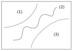
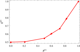
The criteria in Theorem 2.5 are not sharp. Universality class (2) corresponds to a critical surface in the space of parameters $(K_{k})_{k\in N}$ that appears to be rather complicated and certainly is not (!) of the type $\sum_{k\in\mathbb{N}}K_{k}^{-1}=c$ for some $\frac{1}{\sqrt{2}}<c<4$ (see Fig. 6). Note that the full sequence $(K_{k})_{k\in\mathbb{N}}$ determines in which universality class the system is.

Figure 6: Caricature showing the critical surface in the parameter space and the bounds provided by Theorem 2.5.

The behaviour of $K_{k}$ as $k\to\infty$ determines the speed at which $R^{[k]}\to R^{[\infty]}$ in universality classes (2) and (3). Our third theorem provides upper and lower bounds.

Theorem 2.6.

(Bounds for the block synchronization levels)

• In universality classes (2) and (3),

  $$\tfrac{1}{4}\sigma_{k}\leq R^{[k]}-R^{[\infty]}\leq\sqrt{2}\,\sigma_{k},\qquad k\in\mathbb{N}_{0},$$ (2.13)

  with $\sigma_{k}=\sum_{\ell>k}K_{\ell}^{-1}$.

• In universality class (1), the upper bound in (2.13) holds for $k\in\mathbb{N}_{0}$, while the lower bound in (2.13) is replaced by

  $$R^{[k]}-R^{[k_{*}-1]}\geq\tfrac{1}{4}\sum_{\ell=k+1}^{k_{*}-1}K_{\ell}^{-1},\qquad 0\leq k\leq k_{*}-2.$$ (2.14)

  The latter implies that

  $$k_{*}\leq\max\left\{k\in\mathbb{N}\colon\,\sum_{\ell=1}^{k-1}K_{\ell}^{-1}<4\right\}$$ (2.15)

  because $R^{[0]}=1$ and $R^{[k_{*}-1]}>0$.

In universality classes (2) and (3) we have $\lim_{k\to\infty}\sigma_{k}=0$. Depending on how fast $k\mapsto K_{k}$ grows, various speeds of convergence are possible: logarithmic, polynomial, exponential, superexponential.

3 Multi-scaling for the block average phases

In Section 3.1 we explain the heuristics behind Theorem 1.2. The diffusive scaling of the average phase in the mean-field noisy Kuramato model, as shown in the first line of (1.24), is a key tool in our analysis of the multi-scaling of the block average phases in the hierarchical noisy Kuramoto model, stated in Conjecture 2.1. The justification for the latter is given in Section 3.2.

3.1 Diffusive scaling of the average phase for mean-field Kuramato

Proof.

For the heuristic derivation of the second line of (1.24) we combine (1.13)–(1.14), to obtain

$$\frac{\mathrm{d}}{\mathrm{d}t}r(t) =\int_{0}^{2\pi}\mathrm{d}\theta\,\cos\theta$$ (3.1)

$$\qquad\times\left\{-\frac{\partial}{\partial\theta}\,\Big{[}p_{\lambda}(t;\theta)\,\big{\{}Kr(t)\sin[\psi(t)-\theta]\big{\}}\Big{]}+\frac{1}{2}\frac{\partial^{2}}{\partial\theta^{2}}\,p_{\lambda}(t;\theta)\right\}$$

with $\lambda=2Kr$ and $p_{\lambda}(t;\theta)=p_{\lambda}(t;\theta,0)$ (recall that $\omega\equiv 0$). After partial integration with respect to $\theta$ this becomes (use that $\theta\mapsto p_{\lambda}(t;\theta)$ is periodic)

$$\frac{\mathrm{d}}{\mathrm{d}t}r(t)=\int_{0}^{2\pi}\mathrm{d}\theta\,p_{\lambda}(t;\theta)\,\left\{(-\sin\theta)\,Kr(t)\sin(-\theta)+(-\cos\theta)\,\frac{1}{2}\right\},$$ (3.2)

where we use that $\psi(t)=\psi(0)=0$. Define

$$q(t)=\int_{0}^{2\pi}\mathrm{d}\theta\,p_{\lambda}(t;\theta)\,\cos^{2}\theta.$$ (3.3)

Then (3.2) reads

$$\frac{\mathrm{d}}{\mathrm{d}t}r(t)=\left[K(1-q(t))-\frac{1}{2}\right]\,r(t).$$ (3.4)

We know that

$$\lim_{t\to\infty}q(t)=q=\int_{0}^{2\pi}\mathrm{d}\theta\,p_{\lambda}(\theta)\,\cos^{2}\theta$$ (3.5)

with (put $\omega\equiv 0$ in (1.16))

$$p_{\lambda}(\theta)=\frac{\mathrm{e}^{\lambda\cos\theta}}{\int_{0}^{2\pi}\mathrm{d}\phi\,\mathrm{e}^{\lambda\cos\phi}}.$$ (3.6)

Note that $K(1-q)-\frac{1}{2}=0$ because $\lambda=2Kr$ and

$$\int_{0}^{2\pi}\mathrm{d}\theta\,p_{\lambda}(\theta)\sin^{2}\theta=(1/\lambda)\int_{0}^{2\pi}\mathrm{d}\theta\,p_{\lambda}(\theta)\cos\theta=r/\lambda$$ (3.7)

by partial integration. Hence $\lim_{t\to\infty}r(t)=r$. (The fine details of the relaxation are delicate, depend on the full solution of the McKean-Vlasov equation in (1.13), but are of no concern to us here.)

For the derivation of the first line of (1.24) we use the symmetry of the equilibrium distribution (recall (1.16)–(1.17)), i.e.,

$$p_{\lambda}(\theta)=p_{\lambda}(-\theta),$$ (3.8)

together with the fact that $x\mapsto\cos x$ is a symmetric function and $x\mapsto\sin x$ is an asymmetric function.

Write the definition of the order parameter as

$$r_{N}=\frac{1}{N}\sum_{j=1}^{N}\mathrm{e}^{\mathrm{i}(\theta_{j}-\psi_{N})}$$ (3.9)

and compute

$$\frac{\partial r_{N}}{\partial\theta_{i}}=\frac{\mathrm{i}}{N}\,\mathrm{e}^{\mathrm{i}(\theta_{i}-\psi_{N})}-\mathrm{i}\,\frac{\partial\psi_{N}}{\partial\theta_{k}}\,r_{N}.$$ (3.10)

Collecting the real and the imaginary part, we get

$$\frac{\partial\psi_{N}}{\partial\theta_{i}}=\frac{1}{Nr_{N}}\cos(\psi_{N}-\theta_{i}),\qquad\frac{\partial r_{N}}{\partial\theta_{i}}=\frac{1}{N}\sin(\psi_{N}-\theta_{i}).$$ (3.11)

One further differentiation gives

$$\frac{\partial^{2}\psi_{N}}{\partial\theta_{i}^{2}} =-\frac{1}{Nr_{N}^{2}}\frac{\partial r_{N}}{\partial\theta_{i}}\cos(\psi_{N}-\theta_{i})-\frac{1}{Nr_{N}}\left[\frac{\partial\psi_{N}}{\partial\theta_{i}}-1\right]\cos(\psi_{N}-\theta_{i})$$ (3.12)

$$=-\frac{2}{(Nr_{N})^{2}}\sin(\psi_{N}-\theta_{i})\cos(\psi_{N}-\theta_{i})+\frac{1}{Nr_{N}}\sin(\psi_{N}-\theta_{i}),$$

plus a similar formula for $\frac{\partial^{2}r_{N}}{\partial\theta_{i}^{2}}$ (which we will not need). Thus, Itô’s rule applied to (1.6) yields the expression

$$\mathrm{d}\psi_{N}(t)=\sum_{i=1}^{N}\frac{\partial\psi_{N}}{\partial\theta_{i}}(t)\,\mathrm{d}\theta_{i}(t)+\frac{1}{2}\sum_{i=1}^{N}\frac{\partial^{2}\psi_{N}}{\partial\theta_{i}^{2}}(t)\,\big{(}\mathrm{d}\theta_{i}(t)\big{)}^{2}$$ (3.13)

with

$$\frac{\partial\psi_{N}}{\partial\theta_{i}}(t)\, = \frac{1}{Nr_{N}(t)}\cos\big{[}\psi_{N}(t)-\theta_{i}(t)\big{]},$$ (3.14)

$$\frac{\partial^{2}\psi_{N}}{\partial\theta_{i}^{2}}(t) = -\frac{2}{\big{(}Nr_{N}(t))^{2}}\sin\big{[}\psi_{N}(t)-\theta_{i}(t)\big{]}\cos\big{[}\psi_{N}(t)-\theta_{i}(t)\big{]}$$

$$\qquad+\frac{1}{Nr_{N}(t)}\sin\big{[}\psi_{N}(t)-\theta_{i}(t)\big{]}.$$

Inserting (1.7) into (3.13)–(3.1), we get

$$\mathrm{d}\psi_{N}(t)=I(N;t)\,\mathrm{d}t+\mathrm{d}J(N;t)$$ (3.15)

with

$$I(N;t) =\left[\frac{K}{N}-\frac{1}{\big{(}Nr_{N}(t)\big{)}^{2}}\right]\sum_{i=1}^{N}\sin\big{[}\psi_{N}(t)-\theta_{i}(t)\big{]}\cos\big{[}\psi_{N}(t)-\theta_{i}(t)\big{]},$$ (3.16)

$$\mathrm{d}J(N;t) =\frac{1}{Nr_{N}(t)}\sum_{i=1}^{N}\cos\big{[}\psi_{N}(t)-\theta_{i}(t)\big{]}\,\mathrm{d}W_{i}(t),$$

where we use that $\sum_{i=1}^{N}\sin[\psi_{N}(t)-\theta_{i}(t)]=0$ by (1.6). Multiply time by $N$, to get

$$\mathrm{d}\psi_{N}(Nt)=NI(N;Nt)\,\mathrm{d}t+\mathrm{d}J(N;Nt)$$ (3.17)

with

$$NI(N;Nt) =\left[K-\frac{1}{N\big{(}r_{N}(Nt)\big{)}^{2}}\right]\sum_{i=1}^{N}\sin\big{[}\psi_{N}(Nt)-\theta_{i}(Nt)\big{]}\cos\big{[}\psi_{N}(Nt)-\theta_{i}(Nt)\big{]},$$ (3.18)

$$\mathrm{d}J(N;Nt) =\frac{1}{Nr_{N}(Nt)}\sum_{i=1}^{N}\cos\big{[}\psi_{N}(Nt)-\theta_{i}(t)\big{]}\,\mathrm{d}W_{i}(Nt).$$

Suppose that the system converges to a partially synchronized state, i.e., in distribution

$$\lim_{N\to\infty}r_{N}(Nt)=r>0\qquad\forall\,t>0$$ (3.19)

(recall (1.28)). Then $\lim_{N\to\infty}1/N(r_{N}(Nt))^{2}=0$, and so the first line in (3.18) scales like

$$K\sum_{i=1}^{N}\sin\big{[}\psi_{N}(Nt)-\theta_{i}(Nt)\big{]}\cos\big{[}\psi_{N}(Nt)-\theta_{i}(Nt)\big{]},\qquad N\to\infty.$$ (3.20)

This expression is a large sum of terms whose average with respect to the noise is close to zero because of (3.8). Consequently, this sum behaves diffusively. Also the second line in (3.18) behaves diffusively, because it is equal in distribution to

$$\frac{1}{r_{N}(Nt)}\sqrt{\frac{1}{N}\sum_{i=1}^{N}\cos^{2}\big{[}\psi_{N}(Nt)-\theta_{i}(Nt)\big{]}}\,\,\mathrm{d}W_{*}(t).$$ (3.21)

It is shown in [3] that the two terms together lead to the first line of (1.24), i.e., in distribution

$$\lim_{N\to\infty}\psi_{N}(Nt)=\psi_{*}(t)$$ (3.22)

with

$$\psi_{*}(t)=D_{*}\,W_{*}(t),\qquad\psi_{*}(0)=\Phi=0,$$ (3.23)

where $D_{*}=D_{*}(K)$ is the renormalized noise strength given by (1.26) with $D=1$.

Note that the term under the square root in (3.21) converges to $q$ defined in (3.3). The latter holds because $\theta_{i}(Nt)$, $i=1,\ldots,N$, are asymptotically independent and $\theta_{i}(Nt)$ converges in distribution to $\theta\mapsto p_{\lambda}(\theta)$ relative to the value of $\psi_{N}(Nt)$, which itself evolves only slowly (on time scale $Nt$ rather than $t$). ∎

Figure 7: Plot of $\bar{D}_{*}/D_{*}$ as a function of $2Kr$.

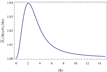
The second line of (3.18) scales in distribution to the diffusion equation

$$\lim_{N\to\infty}\mathrm{d}J(N;Nt)=\bar{D}_{*}\mathrm{d}W_{*}(t),\qquad\bar{D}_{*}=D_{*}(K)=\frac{\sqrt{q}}{r},\qquad r=r(K).$$ (3.24)

Inserting (3.6) and recalling (2.7) and (3.3), we have

$$\bar{D}_{*}=\bar{D}_{*}(K)=\frac{1}{r}\,\sqrt{\frac{I_{2}(2Kr)}{I_{0}(2Kr)}}.$$ (3.25)

Clearly, $D_{*}\neq\bar{D}_{*}$. Interestingly, however,

$$1\leq\frac{\bar{D}_{*}}{D_{*}}\leq C\quad\text{ uniformly in }K\quad\text{ with }C=1.0392\dots$$ (3.26)

(G. Giacomin, private communication). Hence, not only does the first line of (3.18) lower the diffusion constant, the amount by which it does so is less than 4 percent (see Fig. 7). Further thoughts on the reason behind the discrepancy between $D_{*}$ and $\bar{D}_{*}$ can be found in Dahms [4, Section 3.5].

3.2 Multi-scaling of the block average phases for hierarchical Kuramoto

We give the main idea behind Conjecture 2.1. The argument runs along the same line as in Section 3.1, but is more involved because of the hierarchical interaction.

What is crucial for the argument is the separation of space-time scales:

• Each $k$-block consists of $N$ disjoint $(k-1)$-blocks, and evolves on a time scale that is $N$ times larger than the time scale on which the constituent blocks evolve.

• In the limit as $N\to\infty$, the constituent $(k-1)$-blocks in each $k$-block rapidly achieve equilibrium subject to the current value of the $k$-block, which allows us to treat the $k$-blocks as a noisy mean-field Kuramoto model with coefficients that depend on their internal synchronization level, with an effective interaction that depends on the current value of the synchronization level of the $(k+1)$-block.

• The $k$-block itself interacts with the other $k$-block’s, with interaction strength $K_{k+1}$, while the interaction with the even larger blocks it is part of is negligible as $N\to\infty$. This interaction occurs through an effective interaction with the average value of the $k$-blocks which is exactly the value of the $(k+1)$-block.

If we want to observe the evolution of the $k$-blocks labeled $1\leq i\leq N$ that make up the $(k+1)$-block (i.e., the $\Phi_{i}^{[k]}(t)$’s) on time scale $t$), then we must scale the actual oscillator time by $N^{k}$. The synchronization levels within the $\Phi_{i}^{[k]}(t)$’s, given by $R_{i}^{[k]}(Nt)$, are then moving over time $Nt$, since they must be synchronized before the $\Phi_{i}^{[k]}(t)$’s start to diffuse. This is taken care of by our choice of time scales in the hierarchical order parameter (1.36).

Itô’s rule applied to (1.36) with $\eta=0^{\mathbb{N}}$ gives

$$\mathrm{d}\Phi_{0}^{[k]}(t)=\sum_{\zeta\in B_{k}(0)}\frac{\partial\Phi_{0}^{[k]}}{\partial\theta_{\zeta}}(t)\,\mathrm{d}\theta_{\zeta}(N^{k}t)+\frac{1}{2}\sum_{\zeta\in B_{k}(0)}\frac{\partial^{2}\Phi_{0}^{[k]}}{\partial\theta_{\zeta}^{2}}(t)\,\big{(}\mathrm{d}\theta_{\zeta}(N^{k}t)\big{)}^{2}$$ (3.27)

where we have suppressed the $N$-dependence in order to lighten the notation, writing $\Phi_{0}^{[k]}=\Phi_{0,N}^{[k]}$ and $R_{0}^{[k]}=R_{0,N}^{[k]}$. The derivatives are (compare with (3.14))

$$\frac{\partial\Phi_{0}^{[k]}}{\partial\theta_{\zeta}}(t) = \frac{1}{N^{k}R_{0}^{[k]}(Nt)}\cos\big{[}\Phi_{0}^{[k]}(t)-\theta_{\zeta}(N^{k}t)\big{]},$$ (3.28)

$$\frac{\partial^{2}\Phi_{0}^{[k]}}{\partial\theta_{\zeta}^{2}}(t) = -\frac{2}{\big{[}N^{2k}R_{0}^{[k]}(Nt)\big{]}^{2}}\sin\big{[}\Phi_{0}^{[k]}(t)-\theta_{\zeta}(N^{k}t)\big{]}\cos\big{[}\Phi_{0}^{[k]}(t)-\theta_{\zeta}(N^{k}t)\big{]}$$

$$\qquad+\frac{1}{N^{k}R_{0}^{[k]}(Nt)}\sin\big{[}\Phi_{0}^{[k]}(t)-\theta_{\zeta}(N^{k}t)\big{]}.$$

Inserting (1.38), we find

$$d\Phi_{0}^{[k]}(t)=\big{[}I_{1}(k,N;t)+I_{2}(k,N;t)\big{]}\,\mathrm{d}t+\mathrm{d}J(k,N;t)$$ (3.30)

with

$$I_{1}(k,N;t) =\frac{1}{R_{0}^{[k]}(Nt)}\sum_{\ell\in\mathbb{N}}\frac{1}{N^{\ell-1}}\,\Big{(}K_{\ell}-\frac{K_{\ell+1}}{N^{2}}\Big{)}$$ (3.31)

$$\times\sum_{\zeta\in B_{k}(0)}R_{\zeta}^{[\ell]}(N^{1+k-\ell}t)\sin\big{[}\Phi_{\zeta}^{[\ell]}(N^{k-\ell}t)-\theta_{\zeta}(N^{k}t)\big{]}\cos\big{[}\Phi_{0}^{[k]}(t)-\theta_{\zeta}(N^{k}t)\big{]},$$

$$I_{2}(k,N;t) =-\frac{1}{N^{k}\big{[}R_{0}^{[k]}(Nt)\big{]}^{2}}\sum_{\zeta\in B_{k}(0)}\sin\big{[}\Phi_{0}^{[k]}(t)-\theta_{\zeta}(N^{k}t)\big{]}\cos\big{[}\Phi_{0}^{[k]}(t)-\theta_{\zeta}(N^{k}t)\big{]},$$

$$\mathrm{d}J(k,N;t) =\frac{1}{N^{k/2}R_{0}^{[k]}(Nt)}\sum_{\zeta\in B_{k}(0)}\cos\big{[}\Phi_{0}^{[k]}(t)-\theta_{\zeta}(N^{k}t)\big{]}\,\mathrm{d}W_{\zeta}(t).$$

Our goal is to analyse the expressions in (3.31) in the limit as $N\to\infty$, and show that (3.30) converges to the SDE in (2.2) subject to the assumption that the $k$-block converges to a partially synchronized state, i.e.,

$$\lim_{N\to\infty}R_{0}^{[k]}(Nt)=R^{[k]}>0\quad\forall\;t>0.$$ (3.32)

The key idea is that, in the limit as $N\to\infty$, the average phases of the $k$-blocks around $\zeta$ decouple and converge in distribution to $\theta\mapsto p^{[k]}(\theta)$ for all $k\in\mathbb{N}_{0}$, just as for the noisy mean-field Kuramoto model discussed in Section 3.1, with $p^{[k]}(\theta)$ of the same form as $p_{\lambda}(\theta)$ in (3.6) for a suitable $\lambda$ depending on $k$. This is the reason why a recursive structure is in place, captured by the renormalization maps $\mathcal{T}_{K_{k}}$, $k\in\mathbb{N}$.

Along the way we need the quantities

$$R_{0}^{[k]}(Nt) =\frac{1}{N^{k}}\sum_{\zeta\in B_{k}(0)}\cos\big{[}\Phi_{0}^{[k]}(t)-\theta_{\zeta}(N^{k}t)\big{]},$$ (3.33)

$$Q_{0}^{[k]}(Nt) =\frac{1}{N^{k}}\sum_{\zeta\in B_{k}(0)}\cos^{2}\big{[}\Phi_{0}^{[k]}(t)-\theta_{\zeta}(N^{k}t)\big{]}.$$

We also use that for all $k\in\mathbb{N}_{0}$,

$$p^{[k]}(\theta)=p^{[k]}(-\theta),$$ (3.34)

as well as the fact that for all $k\in\mathbb{N}$ and $\ell\geq k$,

$$\begin{array}[]{l}R_{\zeta}^{[\ell]}(Nt)=R_{0}^{[\ell]}(Nt),\\ \Phi_{\zeta}^{[\ell]}(Nt)=\Phi_{0}^{[\ell]}(Nt),\end{array}\qquad\forall\,\zeta\in B_{k}(0).$$ (3.35)

In addition, we use the trigonometric identities

$$\begin{array}[]{ll}\sin(a+b)&=\sin a\cos b+\cos a\sin b,\\ \cos(a+b)&=\cos a\cos b-\sin a\sin b,\end{array}\qquad a,b\in\mathbb{R},$$ (3.36)

to simplify terms via a telescoping argument.

Before we embark on our multi-scale analysis, we note that the expressions in (3.30)–(3.31) simplify somewhat as we take the limit $N\to\infty$. First, in $I_{1}(k,N;t)$ the term $K_{\ell+1}/N^{2}$ is asymptotically negligible compared to $K_{\ell}$, while the sum over $\ell$ can be restricted to $1\leq\ell\leq k+1$ because $|B_{k}(0)|=N^{k}$. Second, $I_{2}(k,N;t)$ is asymptotically negligible because of (3.34) and the fact that $\sin\theta\cos\theta=-\sin(-\theta)\cos(-\theta)$. Thus, we have, in distribution,

$$\mathrm{d}\Phi_{0}^{[k]}(t)=\big{\{}[1+o(1)]\,I_{N}^{[k]}(t)+o(1)\big{\}}\,\mathrm{d}t+\mathrm{d}J_{N}^{[k]}(t),\qquad N\to\infty,$$ (3.37)

with

$$I_{N}^{[k]}(t) =\frac{1}{R_{0}^{[k]}(Nt)}\sum_{\ell=1}^{k+1}\frac{K_{\ell}}{N^{\ell-1}}$$ (3.38)

$$\times\sum_{\zeta\in B_{k}(0)}R_{\zeta}^{[\ell]}(N^{1+k-\ell}t)\sin\big{[}\Phi_{\zeta}^{[\ell]}(N^{k-\ell}t)-\theta_{\zeta}(N^{k}t)\big{]}\cos\big{[}\Phi_{0}^{[k]}(t)-\theta_{\zeta}(N^{k}t)\big{]},$$

$$\mathrm{d}J_{N}^{[k]}(t) =\frac{1}{R_{0}^{[k]}(Nt)}\,\sqrt{Q_{0}^{[k]}(Nt)}\,\mathrm{d}W^{[k]}(t).$$

In the last line we use that $(W_{\zeta}(t))_{t\geq 0}$, $\zeta\in B_{k}(0)$, are i.i.d. and write $(W^{[k]}(t))_{t\geq 0}$ to denote an auxiliary Brownian motion associated with level $k$.

The truncation approximation consists of throwing away the terms with $1\leq\ell\leq k$ and keeping only the terms with $\ell=k+1$.

$\bullet$ Level $k=1$

For $k=1$, by (3.35) the first line of (3.38) reads

$$I_{N}^{[1]}(t)=K_{1}\,\sum_{\zeta\in B_{1}(0)}\sin\big{[}\Phi_{0}^{[1]}(t)-\theta_{\zeta}(Nt)\big{]}\cos\big{[}\Phi_{0}^{[1]}(t)-\theta_{\zeta}(Nt)\big{]}$$ (3.39)

$$\qquad+K_{2}\,\frac{R_{0}^{[2]}(t)}{R_{0}^{[1]}(Nt)}\,\frac{1}{N}\sum_{\zeta\in B_{1}(0)}\sin\big{[}\Phi_{0}^{[2]}(N^{-1}t)-\theta_{\zeta}(Nt)\big{]}\cos\big{[}\Phi_{0}^{[1]}(t)-\theta_{\zeta}(Nt)\big{]}.$$

We telescope the sine. Using (3.36) with $a=\Phi_{0}^{[2]}(N^{-1}t)-\Phi_{0}^{[1]}(t)$ and $b=\Phi_{0}^{[1]}(t)-\theta_{\zeta}(Nt)$, we obtain

$$I_{N}^{[1]}(t) =K_{1}\,\sum_{\zeta\in B_{1}(0)}\sin\big{[}\Phi_{0}^{[1]}(t)-\theta_{\zeta}(Nt)\big{]}\cos\big{[}\Phi_{0}^{[1]}(t)-\theta_{\zeta}(Nt)\big{]}$$ (3.40)

$$\qquad+K_{2}\,\frac{R_{0}^{[2]}(t)}{R_{0}^{[1]}(Nt)}\sin\big{[}\Phi_{0}^{[2]}(N^{-1}t)-\Phi_{0}^{[1]}(t)\big{]}$$

$$\qquad\qquad\times\frac{1}{N}\sum_{\zeta\in B_{1}(0)}\cos^{2}\big{[}\Phi_{0}^{[1]}(t)-\theta_{\zeta}(Nt)\big{]}$$

$$\qquad+K_{2}\,\frac{R_{0}^{[2]}(t)}{R_{0}^{[1]}(Nt)}\ \cos\big{[}\Phi_{0}^{[2]}(N^{-1}t)-\Phi_{0}^{[1]}(t)\big{]}$$

$$\qquad\qquad\times\frac{1}{N}\sum_{\zeta\in B_{1}(0)}\sin\big{[}\Phi_{0}^{[1]}(t)-\theta_{\zeta}(Nt)\big{]}\cos\big{[}\Phi_{0}^{[1]}(t)-\theta_{\zeta}(Nt)\big{]}.$$

On time scale $Nt$, the oscillators in the 1-block have synchronized, and hence the last sum vanishes in the limit $N\to\infty$ by the symmetry property in (3.34) for $k=1$. Therefore we have

$$I_{N}^{[1]}(t) =K_{1}\,\sum_{\zeta\in B_{1}(0)}\sin\big{[}\Phi_{0}^{[1]}(t)-\theta_{\zeta}(Nt)\big{]}\cos\big{[}\Phi_{0}^{[1]}(t)-\theta_{\zeta}(Nt)\big{]}$$ (3.41)

$$\qquad+K_{2}\,\frac{R_{0}^{[2]}(t)\,Q^{[1]}_{0}(Nt)}{R_{0}^{[1]}(Nt)}\sin\big{[}\Phi_{0}^{[2]}(N^{-1}t)-\Phi_{0}^{[1]}(t)\big{]}+o(1).$$

Recalling (3.38) we further have

$$\mathrm{d}J_{N}^{[1]}(t)=\frac{1}{R_{0}^{[1]}(Nt)}\,\sqrt{Q_{0}^{[1]}(Nt)}\,\mathrm{d}W^{[1]}(t)$$ (3.42)

with

$$Q_{0}^{[1]}(Nt)=\frac{1}{N}\sum_{\zeta\in B_{1}(0)}\cos^{2}\big{[}\Phi_{0}^{[1]}(t)-\theta_{\zeta}(Nt)\big{]}.$$ (3.43)

The first term in the right-hand side of (3.41) is the same as that in (3.20) with $K=K_{1}$ and $\psi_{N}(Nt)=\Phi_{0}^{[1]}(t)$. The term in the right-hand side of (3.42) is the same as that of (3.21) with $r_{N}(Nt)=R_{0}^{[1]}(Nt)$ and $W_{*}(t)=W^{[1]}(t)$. Together they produce, in the limit as $N\to\infty$, the same noise term as in the mean-field model, namely,

$$\mathcal{D}^{[1]}\,\mathrm{d}W^{[1]}(t)$$ (3.44)

with a renormalized noise strength

$$\mathcal{D}^{[1]}=D_{*}(K_{1})$$ (3.45)

given by (1.26) with $D=1$, where we use that

$$\lim_{N\to\infty}R_{0}^{[1]}(Nt)=R^{[1]}=R^{[1]}(K_{1}),\quad\lim_{N\to\infty}Q_{0}^{[1]}(Nt)=Q^{[1]}=Q^{[1]}(K_{1})\quad\forall\;t>0.$$ (3.46)

The second term in the right-hand side of (3.41) is precisely the Kuramoto-type interaction term of $\Phi_{0}^{[1]}(t)$ with the average phase of the oscillators in the 2-block at time $Nt$. Therefore, in the limit as $N\to\infty$, we end up with the limiting SDE

$$\mathrm{d}\Phi_{0}^{[1]}(t)=K_{2}\,\mathcal{E}^{[1]}\,R_{0}^{[2]}(t)\,\sin\big{[}\Phi-\Phi_{0}^{[1]}(t)\big{]}+\mathcal{D}^{[1]}\,\mathrm{d}W^{[1]}(t)$$ (3.47)

with

$$\mathcal{E}^{[1]}=\frac{Q^{[1]}}{R^{[1]}}.$$ (3.48)

If we leave out the first term in the right-hand side of (3.41) (which as shown in (3.26) may be done at the cost of an error of less than 4 percent), then we end up with the limiting SDE

$$\mathrm{d}\Phi_{0}^{[1]}(t)=K_{2}\,\bar{\mathcal{E}}^{[1]}\,R_{0}^{[2]}(t)\,\sin\big{[}\Phi-\Phi_{0}^{[1]}(t)\big{]}+\bar{\mathcal{D}}^{[1]}\,\mathrm{d}W^{[1]}(t)$$ (3.49)

with $\bar{\mathcal{E}}^{[1]}=\mathcal{E}^{[1]}$ and

$$\bar{\mathcal{D}}^{[1]}=\bar{D}_{*}(K_{1})=\frac{\sqrt{Q^{[1]}}}{R^{[1]}}$$ (3.50)

given by (3.25) with $D=1$. Thus we have justified the SDE in (2.10) for $k=1$. After a transient period we have $\lim_{t\to\infty}R_{0}^{[2]}(t)=R_{0}^{[2]}$.

Note that, in the approximation where we leave out the first term in the right-hand side of (3.41), the pair $(R^{[1]},Q^{[1]})$ takes over the role of the pair $(r,q)$ in the mean-field model. The latter are the unique solution of the consistency relation and recursion relation (recall (2.7), (3.6), (3.7) and (3.24))

$$r=\frac{I_{1}(2Kr)}{I_{0}(2Kr)},\qquad q=\frac{I_{2}(2Kr)}{I_{0}(2Kr)}.$$ (3.51)

These can be summarised as saying that $(r,q)=\mathcal{T}_{K}(1,1)$, with $\mathcal{T}_{K}$ the renormalization map introduced in Definition 2.2. Thus we see that

$$(R^{[1]},Q^{[1]})=\mathcal{T}_{K_{1}}(1,1),$$ (3.52)

which explains why $\mathcal{T}_{K_{1}}$ comes on stage.

$\bullet$ Levels $k\geq 2$

For $k\geq 2$, by (3.35) the term with $\ell=k+1$ in $I_{N}^{[k]}(t)$ in the first line of (3.38) equals

$$I_{N}^{[k]}(t)|_{\ell=k+1}$$ (3.53)

$$=K_{k+1}\,\frac{R_{0}^{[k+1]}(t)}{R_{0}^{[k]}(Nt)}\,\frac{1}{N^{k}}\sum_{\zeta\in B_{k}(0)}\sin\big{[}\Phi_{0}^{[k+1]}(N^{-1}t)-\theta_{\zeta}(N^{k}t)\big{]}\cos\big{[}\Phi_{0}^{[k]}(t)-\theta_{\zeta}(N^{k}t)\big{]}.$$

We again telescope the sine. Using (3.36), this time with $a=\Phi_{0}^{[k+1]}(N^{-1}t)-\Phi_{0}^{[k]}(t)$ and $b=\Phi_{0}^{[k]}(t)-\theta_{\zeta}(N^{k}t)$, we can write

$$I_{N}^{[k]}(t)|_{\ell=k+1} =K_{k+1}\,\frac{R_{0}^{[k+1]}(t)}{R_{0}^{[k]}(Nt)}\sin\big{[}\Phi_{0}^{[k+1]}(N^{-1}t)-\Phi_{0}^{[k]}(t)\big{]}$$ (3.54)

$$\qquad\qquad\times\frac{1}{N^{k}}\sum_{\zeta\in B_{k}(0)}\cos^{2}\big{[}\Phi_{0}^{[k]}(t)-\theta_{\zeta}(N^{k}t)\big{]}$$

$$\qquad+K_{k+1}\,\frac{R_{0}^{[k+1]}(t)}{R_{0}^{[k]}(Nt)}\sin\big{[}\Phi_{0}^{[k+1]}(N^{-1}t)-\Phi_{0}^{[k]}(t)\big{]}$$

$$\qquad\qquad\times\frac{1}{N^{k}}\sum_{\zeta\in B_{k}(0)}\sin\big{[}\Phi_{0}^{[k]}(t)-\theta_{\zeta}(N^{k}t)\big{]}\cos\big{[}\Phi_{0}^{[k]}(t)-\theta_{\zeta}(N^{k}t)\big{]}.$$

By the symmetry property in (3.34), the last term vanishes as $N\to\infty$, and so we have

$$I_{N}^{[k]}(t)|_{\ell=k+1}=K_{k+1}\,\frac{R_{0}^{[k+1]}(t)\,Q^{[k]}_{0}(Nt)}{R_{0}^{[k]}(Nt)}\,\sin\big{[}\Phi_{0}^{[k+1]}(N^{-1}t)-\Phi_{0}^{[k]}(t)\big{]}+o(1).$$ (3.55)

Using that

$$\lim_{N\to\infty}R_{0}^{[k]}(Nt)=R^{[k]},\qquad\lim_{N\to\infty}Q_{0}^{[k]}(Nt)=Q^{[k]}\qquad\forall\,t>0,$$ (3.56)

we obtain

$$I_{N}^{[k]}(t)|_{\ell=k+1}=K_{k+1}\,\frac{Q^{[k]}}{R^{[k]}}\,R_{0}^{[k+1]}(t)\,\sin\big{[}\Phi-\Phi_{0}^{[k]}(t)\big{]}+o(1),$$ (3.57)

which is the Kuramoto-type interaction term of $\Phi_{0}^{[k]}(t)$ with the average phase of the oscillators in the $(k+1)$-block at time $N^{k}t$. The noise term in (3.38) scales like

$$\mathrm{d}J_{N}^{[k]}(t)=\frac{1}{R^{[k]}}\,\sqrt{Q^{[k]}}\,\mathrm{d}W^{[k]}(t)+o(1).$$ (3.58)

Hence we end up with

$$I_{N}^{[k]}(t)|_{\ell=k+1}\mathrm{d}t+\mathrm{d}J_{N}^{[k]}(t)=K_{k+1}\,\frac{Q^{[k]}}{R^{[k]}}\,R_{0}^{[k+1]}(t)\,\sin\big{[}\Phi-\Phi_{0}^{[k]}(t)\big{]}+\frac{\sqrt{Q^{[k]}}}{R^{[k]}}\,\mathrm{d}W^{[k]}(t)+o(1).$$ (3.59)

Thus we have justified the SDE in (2.10) for $k\geq 2$, with $\bar{\mathcal{E}}^{[k]}$ and $\bar{\mathcal{D}}^{[k]}$ given by (2.11). Note that

$$(R^{[k]},Q^{[k]})=\mathcal{T}_{K_{k}}(R^{[k-1]},Q^{[k-1]}),$$ (3.60)

in full analogy with (3.52).

For $k\geq 2$ the term with $\ell=k$ equals

$$I_{N}^{[k]}(t)|_{\ell=k}=K_{k}\sum_{i=1}^{N}\frac{1}{N^{k-1}}\sum_{\zeta\in B_{k-1}(i)}\\ \sin\big{[}\Phi_{0}^{[k]}(t)-\theta_{\zeta}(N^{k}t)\big{]}\cos\big{[}\Phi_{0}^{[k]}(t)-\theta_{\zeta}(N^{k}t)\big{]},$$ (3.61)

where $B_{k-1}(i)$, $1\leq i\leq N$, are the $(k-1)$-blocks making up the $k$-block $B_{k}(0)$, and we use that $(R_{\zeta}^{[k]}(t),\Phi_{\zeta}^{[k]}(t))=(R_{0}^{[k]}(t),\Phi_{0}^{[k]}(t))$ for all $\zeta\in B_{k-1}(i)$ and all $1\leq i\leq N$. The sum in (3.61) has a similar form as the first term in the right-hand side of (3.41), but now with the $1$-block replaced by $N$ copies of $(k-1)$-blocks. This opens up the possibility of a finer approximation analogous to the one obtained by using (3.45) instead of (3.50). As we argued in Section 3.1, the improvement should be minor (recall (3.26)).

4 Universality classes and synchronization levels

In Section 4.1 we derive some basic properties of the renormalization map (Lemmas 4.1–4.3 below). In Section 4.2 we prove Theorem 2.5. The proof relies on convexity and sandwich estimates (Lemmas 4.4–4.6 below).

4.1 Properties of the renormalization map

For $\lambda\in[0,\infty)$, define

$$V(\lambda) =\int_{0}^{2\pi}\mathrm{d}\theta\,\cos\theta\,p_{\lambda}(\theta)=\frac{I_{1}(\lambda)}{I_{0}(\lambda)},$$ (4.1)

$$W(\lambda) =\int_{0}^{2\pi}\mathrm{d}\theta\,\cos^{2}\theta\,p_{\lambda}(\theta)=\frac{I_{2}(\lambda)}{I_{0}(\lambda)},$$

where the probability distribution $p_{\lambda}(\theta)$ is given by (1.16) with $\omega\equiv 0$ and $D=1$. The renormalization map $\mathcal{T}_{K}$ in (2.8) can be written as $(\bar{R},\bar{Q})=\mathcal{T}_{K}(R,Q)$ with

$$\bar{R} =RV(\lambda),$$

$$\bar{Q}-\tfrac{1}{2} =(Q-\tfrac{1}{2})\big{[}2W(\lambda)-1\big{]},$$ (4.2)

and $\lambda=2K\bar{R}\sqrt{Q}$. It is known that $\lambda\mapsto V(\lambda)$ is strictly increasing and strictly convex, with $V(0)=0$ and $\lim_{\lambda\to\infty}V(\lambda)=1$.

Lemma 4.1.

The map $K\mapsto\bar{R}(R,K)$ is strictly increasing.

Proof.

The derivative of $\bar{R}$ w.r.t. $K$ exists by the implicit function theorem, so that

$$\frac{d\bar{R}}{dK}=2RV^{\prime}(2K\bar{R})\,\left[\bar{R}+K\frac{d\bar{R}}{dK}\right],$$

$$\frac{d\bar{R}}{dK}\,\big{[}1-2KRV^{\prime}(2K\bar{R})\big{]}=2R\bar{R}V^{\prime}(2K\bar{R}).$$ (4.3)

Note that $\bar{R}$ is the solution to $\bar{R}=RV(2K\bar{R})$, which is non-trivial only when $1<2RKV^{\prime}(2K\bar{R})$ due to the concavity of the map $R\mapsto RV(2K\bar{R})$. This implies that $2KRV^{\prime}(2K\bar{R})<1$ at the solution, which makes the term in (4.1) between square brackets positive. The claim follows since we proved previously that $R,\bar{R}\in[0,1)$ and $V^{\prime}(2K\bar{R})>0$. ∎

Lemma 4.2.

The map $K\mapsto\bar{Q}(\bar{R},K,Q)$ is strictly increasing.

Proof.

The derivative of $\bar{Q}$ w.r.t. $K$ exists by the implicit function theorem, so that

$$\frac{d\bar{Q}}{dK}=(Q-\tfrac{1}{2})\,4\sqrt{Q}\,W^{\prime}\big{(}2\sqrt{Q}K\bar{R}\big{)}\,\left[\bar{R}+K\frac{d\bar{R}}{dK}\right].$$ (4.4)

We have that $(Q-\tfrac{1}{2})\sqrt{Q}\geq 0$ because $Q\in[\frac{1}{2},1)$, $W^{\prime}(2\sqrt{Q}K\bar{R})>0$ as proven before, and $[\bar{R}+K\frac{d\bar{R}}{dK}]>0$ as in the proof of Lemma 4.1. The claim therefore follows. ∎

Lemma 4.3.

The map $(R,Q)\mapsto(\bar{R},\bar{Q})$ is non-increasing in both components, i.e.,

1. $R\mapsto\bar{R}(K,R)$ is non-increasing.

2. $Q\mapsto\bar{Q}(K,\bar{R},Q)$ is non-increasing.

Proof.

(i) We have

$$\bar{R}=R\,V\big{(}2\sqrt{Q}K\bar{R}\big{)}.$$ (4.5)

But $V(\sqrt{Q}K\bar{R})\in[0,1)$, and so $\bar{R}\leq R$.
(ii) We have

$$\bar{Q}-\tfrac{1}{2}=(Q-\tfrac{1}{2})\,\big{[}2W\big{(}2\sqrt{Q}K\bar{R}\big{)}-1\big{]}.$$ (4.6)

But $W(2\sqrt{Q}K\bar{R})\in[\frac{1}{2},1)$, and so $\bar{Q}\leq Q$. In fact, since both $V(2\sqrt{Q}K\bar{R})$ and $W(2\sqrt{Q}K\bar{R})$ are $<1$, both maps are strictly decreasing until $R=0$ and $Q=\tfrac{1}{2}$ are hit, respectively. ∎

4.2 Renormalization

Recall (2.7). To prove Theorems 2.5 we need the following lemma.

Lemma 4.4.

The map $\lambda\mapsto\log I_{0}(\lambda)$ is analytic, strictly increasing and strictly convex on $(0,\infty)$, with

$$I_{0}(\lambda)=1+\tfrac{1}{4}\lambda^{2}\,[1+O(\lambda^{2})],\quad\lambda\downarrow 0,\qquad I_{0}(\lambda)=\frac{\mathrm{e}^{\lambda}}{\sqrt{2\pi\lambda}}\,[1+O(\lambda^{-1})],\quad\lambda\to\infty.$$ (4.7)

∎

Proof.

Analyticity is immediate from (2.7). Strict convexity follows because the numerator of $[\log I_{0}(\lambda)]^{\prime\prime}$ equals

$$I_{2}(\lambda)I_{0}(\lambda)-I_{1}(\lambda)I_{1}(\lambda) =\frac{1}{2\pi}\int_{0}^{2\pi}\mathrm{d}\phi\int_{0}^{2\pi}\mathrm{d}\psi\,[\cos^{2}\phi-\cos\phi\cos\psi]\,\mathrm{e}^{\lambda(\cos\phi+\cos\psi)}$$ (4.8)

$$=\frac{1}{2\pi}\int_{0}^{2\pi}\mathrm{d}\phi\int_{0}^{2\pi}\mathrm{d}\psi\,[\cos\phi-\cos\psi]^{2}\,\mathrm{e}^{\lambda(\cos\phi+\cos\psi)}>0,$$

where we symmetrize the integrand. Since $\log I_{0}(0)=0$, $\log I_{0}(\lambda)>0$ for $\lambda>0$ and $\lim_{\lambda\to\infty}\log I_{0}(\lambda)=\infty$, the strict monotonicity follows. The asymptotics in (4.7) is easily deduced from (2.7) via a saddle point computation. ∎

Since $V=I_{1}/I_{0}=[\log I_{0}]^{\prime}$, we obtain from (4.7) and convexity that

$$V(\lambda) \sim \tfrac{1}{2}\lambda,\qquad\lambda\downarrow 0,$$ (4.9)

$$1-V(\lambda) \sim \frac{1}{2\lambda},\qquad\lambda\to\infty.$$ (4.10)

This limiting behaviour of $V(\lambda)$ inspires the choice of bounding functions in the next lemma.

Lemma 4.5.

$V^{+}(\lambda)\geq V(\lambda)\geq V^{-}(\lambda)$ for all $\lambda\in(0,\infty)$ with (see Fig. 8)

$$V^{+}(\lambda) =\frac{2\lambda}{1+2\lambda},$$ (4.11)

$$V^{-}(\lambda) =\frac{\tfrac{1}{2}\lambda}{1+\tfrac{1}{2}\lambda}.$$

∎

Proof.

Segura [14, Theorem 1] shows that

$$V(\lambda)<V_{*}^{+}(\lambda)=\frac{\lambda}{\tfrac{1}{2}+\sqrt{(\tfrac{1}{2})^{2}+\lambda^{2}}},\qquad\lambda>0.$$ (4.12)

Since $\lambda<\sqrt{(\tfrac{1}{2})^{2}+\lambda^{2}}$, it follows that $V_{*}^{+}(\lambda)<V^{+}(\lambda)$. Laforgia and Natalini [10, Theorem 1.1] show that

$$V(\lambda)>V_{*}^{-}(\lambda)=\frac{-1+\sqrt{\lambda^{2}+1}}{\lambda},\qquad\lambda>0.$$ (4.13)

Abbreviate $\eta=\sqrt{\lambda^{2}+1}$. Then $\lambda=\sqrt{(\eta-1)(\eta+1)}$, and we can write

$$V_{*}^{-}(\lambda)=\sqrt{\frac{\eta-1}{\eta+1}}=\frac{\lambda}{\eta+1}=\frac{\lambda}{2+(\eta-1)}.$$ (4.14)

Since $\lambda>\eta-1$, it follows that $V_{*}^{-}(\lambda)>V^{-}(\lambda)$. ∎

Figure 8: Plots of the tighter bounds in the proof of Lemma 4.5 and the looser bounds needed for the proof of Theorem 2.5.

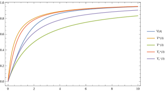
Note that both $V^{+}$ and $V^{-}$ are strictly increasing and concave on $(0,\infty)$, which guarantees the uniqueness and non-triviality of the solution to the consistency relation in the first line of (4.1) when we replace $V(\lambda)$ by either $V^{+}(\lambda)$ or $V^{-}(\lambda)$.

In the sequel we write $V,W,R_{k},Q_{k}$ instead of $V_{\delta_{0}},W_{\delta_{0}},R^{[k]},Q^{[k]}$ to lighten the notation. We know that $(R_{k})_{k\in\mathbb{N}_{0}}$ is the solution of the sequence of consistency relations

$$R_{k+1}=R_{k}V\big{(}2\sqrt{Q_{k}}K_{k+1}R_{k+1}\big{)},\qquad k\in\mathbb{N}_{0}.$$ (4.15)

This requires as input the sequence $(Q_{k})_{k\in\mathbb{N}_{0}}$, which is obtained from the sequence of recursion relations

$$Q_{k+1}-\tfrac{1}{2}=(Q_{k}-\tfrac{1}{2})\big{[}2W\big{(}2\sqrt{Q_{k}}K_{k+1}R_{k+1}\big{)}-1\big{]}.$$ (4.16)

By using that $Q_{k}\in[\frac{1}{2},1]$ for all $k\in\mathbb{N}_{0}$, we can remove $Q_{k}$ from (4.15) at the cost of doing estimates. Namely, let $(R_{k}^{+})_{k\in\mathbb{N}_{0}}$ and $(R_{k}^{-})_{k\in\mathbb{N}_{0}}$ denote the solutions of the sequence of consistency relations

$$\begin{array}[]{lll}R^{+}_{k+1}&=R_{k}V^{+}\big{(}2K_{k+1}R^{+}_{k+1}\big{)},&k\in\mathbb{N}_{0},\\ R^{-}_{k+1}&=R_{k}V^{-}\big{(}2\sqrt{\tfrac{1}{2}}K_{k+1}R^{-}_{k+1}\big{)},&k\in\mathbb{N}_{0}.\end{array}$$ (4.17)

Lemma 4.6.

$R_{k}^{+}\geq R_{k}\geq R^{-}_{k}$ for all $k\in\mathbb{N}$. ∎

Proof.

If we replace $V(\lambda)$ by $V^{+}(\lambda)$ (or $V^{-}(\lambda)$) in the consistency relation for $R_{k+1}$ given by (4.15), then the new solution $R_{k+1}^{+}$ (or $R^{-}_{k+1}$) is larger (or smaller) than $R_{k+1}$. Indeed, we have

$$R_{k+1}=R_{k}V(2K_{k+1}R_{k+1}\sqrt{Q_{k}})\leq R_{k}V^{+}(2K_{k+1}R_{k+1}).$$ (4.18)

Because $V^{+}$ is concave, it follows from (4.18) and the first line of (4.17) that $R_{k+1}\leq R^{+}_{k+1}$. ∎

We are now ready to prove Theorems 2.5–2.6.

Proof.

From the first lines of (4.11) and (4.17) we deduce

$$R_{k}>\frac{1}{4K_{k+1}}\quad\Longleftrightarrow\quad R_{k+1}^{+}>0\quad\Longrightarrow\quad R_{k}-R_{k+1}^{+}=\frac{1}{4K_{k+1}}.$$ (4.19)

Hence, with the help of Lemma 4.6, we get

$$R_{k}>\frac{1}{4K_{k+1}}\quad\Longrightarrow\quad R_{k}-R_{k+1}\geq\frac{1}{4K_{k+1}}.$$ (4.20)

Iteration gives (recall that $R_{0}=1$)

$$1-R_{k}\geq\min\left\{1,\sum_{\ell=1}^{k}\frac{1}{4K_{\ell}}\right\}.$$ (4.21)

As soon as the sum in the right-hand side is $\geq 1$, we know that $R_{k}=0$. This gives us the criterion for universality class (1) in Theorem 2.5. Similarly, from the second lines of (4.11) and (4.17) we deduce

$$R_{k}>\frac{2\sqrt{2}}{K_{k+1}}\quad\Longleftrightarrow\quad R_{k+1}^{-}>0\quad\Longrightarrow\quad R_{k}-R_{k+1}^{-}=\frac{\sqrt{2}}{K_{k+1}}.$$ (4.22)

Hence, with the help of Lemma 4.6, we get

$$R_{k}>\frac{\sqrt{2}}{K_{k+1}}\quad\Longrightarrow\quad R_{k}-R_{k+1}\leq\frac{\sqrt{2}}{K_{k+1}}.$$ (4.23)

Iteration gives

$$1-R_{k}\leq\max\left\{1,\sum_{\ell=1}^{k}\frac{\sqrt{2}}{K_{\ell}}\right\}.$$ (4.24)

As soon as the sum in the right-hand side is $<1$, we know that $R_{k}>0$. This gives us the criterion for universality class (3) in Theorem 2.5.

In universality classes (2) and (3) we have $R_{k}^{+}\geq R_{k}>0$ for $k\in\mathbb{N}$, and hence

$$R_{k}-R_{\infty}=\sum_{\ell\geq k}(R_{\ell}-R_{\ell+1})\geq\sum_{\ell\geq k}(R_{\ell}-R_{\ell+1}^{+})=\sum_{\ell\geq k}\frac{1}{4K_{\ell+1}},\qquad k\in\mathbb{N}_{0}.$$ (4.25)

In universality class (1), on the other hand, we have $R_{k}^{+}\geq R_{k}>0$ for $1\leq k<k_{*}$ and $R_{k}=0$ for $k\geq k_{*}$, and hence

$$R_{k}-R_{k_{*}-1}=\sum_{\ell=k}^{k_{*}-2}(R_{\ell}-R_{\ell+1})\geq\sum_{\ell=k}^{k_{*}-2}(R_{\ell}-R_{\ell+1}^{+})=\sum_{\ell=k}^{k_{*}-2}\frac{1}{4K_{\ell+1}},\qquad 0\leq k\leq k_{*}-2.$$ (4.26)

Finally, with no assumption on $(R_{k})_{k\in\mathbb{N}}$, we have

$$R_{k}-R_{\infty}=\sum_{\ell\geq k}(R_{\ell}-R_{\ell+1})\leq\sum_{\ell\geq k}(R_{\ell}-R_{\ell+1}^{-})\leq\sum_{\ell\geq k}\frac{\sqrt{2}}{K_{\ell+1}},$$ (4.27)

where the last inequality follows from (4.22). The bounds in (4.25)–(4.27) yields the sandwich in Theorem 2.6. ∎

Remark 4.7.

In the proof of Theorem 2.5–2.6 we exploited the fact that $Q_{k}\in[\tfrac{1}{2},1]$ to get estimates that involve a consistency relation in only $R_{k}$. In principle we can improve these estimates by exploring what effect $Q_{k}$ has on $R_{k}$. Namely, in analogy with Lemma 4.5, we have $W^{+}(\lambda)\geq W(\lambda)\geq W^{-}(\lambda)$ for all $\lambda\in(0,\infty)$ with (see Fig. 9)

$$W^{+}(\lambda)=\frac{1+\lambda}{2+\lambda},\qquad W^{-}(\lambda)=\frac{1-\lambda+\lambda^{2}}{2+\lambda^{2}}.$$ (4.28)

This allows for better control on $Q_{k}$ and hence better control on $R_{k}$. However, the formulas are cumbersome to work with and do not lead to a sharp condition anyway. ∎

Figure 9: Bounding functions for $W(\lambda)$.

Appendix A Numerical analysis

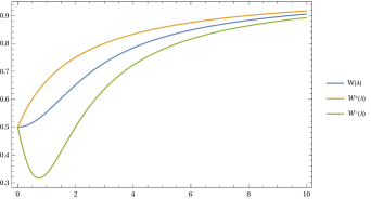
In this appendix we numerically compute the iterates of the renormalization map in (2.8) for two specific choices of $(K_{k})_{k\in\mathbb{N}}$, belonging to universality classes (1) and (3), respectively.

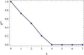
In Fig. 10 we show an example in universality class (1): $K_{k}=\frac{3}{2\log 2}\log(k+1)$. Synchronization is lost at level $k=4$. When we calculate the sum that appears in our sufficient criterion for universality class (1), stated in Theorem 2.5, up to level $k=4$, we find that

$$\sum_{k=1}^{4}\frac{2\log 2}{3\log(k+1)}=1.70774.$$ (A.1)

This does not exceed $4$, which shows that our sufficient criterion is not tight. It only gives us an upper bound for the level above which synchronization is lost for sure (recall (2.15)), although it may be lost earlier.

Figure 10: A plot of the renormalization map $(R^{[k]},Q^{[k]})$ for $k=0,\ldots,7$ (left) and the corresponding values of $R^{[k]}$ (right) for the choice $K_{k}=\frac{3}{2\log 2}\log(k+1)$.

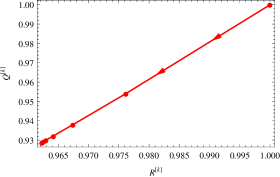
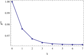
In Fig. 11 we show an example of universality class (3), where $K_{k}=4\,\mathrm{e}^{k}$. There is synchronization at all levels. To check our sufficient criterion we calculate the sum

$$\sum_{k\in\mathbb{N}}\frac{1}{4\,\mathrm{e}^{k}}\approx 0.145494<\frac{1}{\sqrt{2}}\approx 0.7071.$$ (A.2)

Figure 11: A plot of the renormalization map $(R^{[k]},Q^{[k]})$ for $k=0,\ldots,7$ (left) and the corresponding values of $R^{[k]}$ (right) for the choice $K_{k}=4\,\mathrm{e}^{k}$.

To find a sequence $(K_{k})_{k\in\mathbb{N}}$ for universality class (2) is difficult because we do not know the precise criterion for criticality. An artificial way of producing such a sequence is to calculate the critical interaction strength at each hierarchical level and taking the next interaction strength to be $1$ larger.

References

- [1] J.A. Acebrón, L.L. Bonilla, C.J. Pérez Vicente, F. Ritort and R. Spigler, The Kuramoto model: A simple paradigm for synchronization phenomena, Rev. Mod. Phys. 77 (2005) 137–185.
- [2] A. Arenas, A. Díaz-Guilera, J. Kurths, Y. Moreno and C. Zhou, Synchronization in complex networks, Physics Reports 469 (2008) 93–153.
- [3] L. Bertini, G. Giacomin and C. Poquet, Synchronization and random long time dynamics for mean-field plane rotators, Probab. Theory Relat. Fields 160 (2014) 593–653.
- [4] R. Dahms, Long-time behavior of a spherical mean field model, PhD thesis at Technical University Berlin, 2002 (unpublished).
- [5] P. Dai Pra and F. den Hollander, McKean-Vlasov limit for interacting random processes in random media, J. Stat. Phys. 84 (1996) 735–772.
- [6] S. Ha and M. Slemrod, A fast-slow dynamical systems theory for the Kuramoto type phase model, J. Differ. Equ. 251 (2011) 2685–2695.
- [7] I. Karatzas and S.E. Shreve, Brownian Motion and Stochastic Calculus, Graduate Texts in Mathematics 113 (2nd. ed.), Springer, New York, 1998.
- [8] Y. Kuramoto, Self-entrainment of a population of coupled non-linear oscillators. In: International Symposium on Mathematical Problems in Theoretical Physics, pp. 420–422. Lecture Notes in Phys. 39, Springer, Berlin, 1975.
- [9] Y. Kuramoto, Chemical Oscillations, Waves, and Turbulence, Springer, New York, 1984.
- [10] A. Laforgia and P. Natalini, Some inequalities for modified bessel functions, J. Ineq. App. 2010, article 253035 (2010) 1–10.
- [11] E. Luçon, Oscillateurs couplés, désordre et renormalization, PhD thesis, Université Pierre et Marie Curie-Paris VI, 2012.
- [12] E. Luçon and C. Poquet, Long time dynamics and disorder-induced traveling waves in the stochastic Kuramoto model, Ann. Inst. H. Poincaré Probab. Statist. 53 (2017) 1196–1240.
- [13] H. Sakaguchi, Cooperative phenomena in coupled oscillators systems under external fields, Prog. Theor. Phys. 79 (1988) 39–46.
- [14] J. Segura, Bounds for ratios of modified Bessel functions and associated Turin-type inequalities, J. Math. An. App. 372 (2011) 516–528.
- [15] B. Sonnenschein and L. Schimansky-Geier, Approximate solution to the stochastic Kuramoto model, Phys. Rev. E 88, 052111 (2013) 1–5.
- [16] S.H. Strogatz, From Kuramoto to Crawford: Exploring the onset of synchronization in populations of coupled oscillators, Phys. D 143 (2000) 1–20.
- [17] S.H. Strogatz and R.E. Mirollo, Stability of incoherence in a population of coupled oscillators, J. Stat. Phys. 63 (1991) 613–635.
- [18] S.H. Strogatz, R.E. Mirollo and P.C. Matthews, Coupled nonlinear oscillators below the synchronization threshold: relaxation by generalized Landau damping, Phys. Rev. Lett. 68 (1992) 2730–2733.
- [19] A.T. Winfree, Biological rhythms and the behavior of populations of coupled oscillators, J. Theor. Biol. 16 (1967)15–42.
- [20] A.T. Winfree, The Geometry of Biological Time, Springer, New York, 1980.