NoScope: Optimizing Neural Network Queries
over Video at Scale

Abstract

Recent advances in computer vision—in the form of deep neural networks—have made it possible to query increasing volumes of video data with high accuracy. However, neural network inference is computationally expensive at scale: applying a state-of-the-art object detector in real time (i.e., 30+ frames per second) to a single video requires a $4000 GPU. In response, we present NoScope, a system for querying videos that can reduce the cost of neural network video analysis by up to three orders of magnitude via inference-optimized model search. Given a target video, object to detect, and reference neural network, NoScope automatically searches for and trains a sequence, or cascade, of models that preserves the accuracy of the reference network but is specialized to the target video and are therefore far less computationally expensive. NoScope cascades two types of models: specialized models that forego the full generality of the reference model but faithfully mimic its behavior for the target video and object; and difference detectors that highlight temporal differences across frames. We show that the optimal cascade architecture differs across videos and objects, so NoScope uses an efficient cost-based optimizer to search across models and cascades. With this approach, NoScope achieves two to three order of magnitude speed-ups (265-15,500$\times$ real-time) on binary classification tasks over fixed-angle webcam and surveillance video while maintaining accuracy within 1-5% of state-of-the-art neural networks.

1 Introduction

Video represents a rich source of high-value, high-volume data: video comprised over 70% of all Internet traffic [2] in 2015 and over 300 hours of video are uploaded to YouTube every minute [3]. We can leverage this video data to answer queries about the physical world, our lives and relationships, and our evolving society.

Figure 1: NoScope is a system for accelerating neural network analysis over videos via inference-optimized model search. Given an input video, target object, and reference neural network, NoScope automatically searches for and trains a cascade of models—including difference detectors and specialized networks—that can reproduce the binarized outputs of the reference network with high accuracy—but up to three orders of magnitude faster.

It is increasingly infeasible—both too costly and too slow—to rely on manual, human-based inspection of large-scale video data. Thus, automated analysis is critical to answering these queries at scale. The literature offers a wealth of proposals for storing and querying [7, 59, 101, 73, 6, 36, 57, 38, 48, 94] videos, largely based on classical computer vision techniques. In recent times, however, deep neural networks (NNs) [58, 40, 66, 44, 67] have largely displaced classical computer vision methods due to their incredible accuracy—often rivaling or exceeding human capabilities—in visual analyses ranging from object classification [82] to image-based cancer diagnosis [31, 95].

Unfortunately, applying NNs to video data is prohibitively expensive at scale. The fastest NNs for accurate object detection run at 30-80 frames per second (fps), or 1-2.5$\times$ real time (e.g., 50 fps on an NVIDIA K80 GPU, ~$4000 retail, $0.70-0.90 per hour on cloud; 80 fps on an NVIDIA P100, ~$4600 retail) [80, 79, 81]. Given continued decreases in image sensor costs (e.g., < $0.65 for a 640x480 VGA CMOS sensor), the computational overheads of NNs lead to a three order-of-magnitude imbalance between the cost of data acquisition and the cost of data processing. Moreover, state-of-the-art NNs continue to get deeper and more costly to evaluate; for example, Google’s winning NN in the 2014 ImageNet competition had 22 layers; Microsoft’s winning NN in 2015 had 152 layers [44].

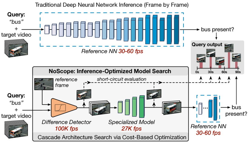
In response, we present NoScope, a system for querying videos that can reduce the cost of NN-based analysis by up to three orders of magnitude via inference-optimized model search. Our NoScope prototype supports queries in the form of the presence or absence of a particular object class. Given a query consisting of a target video, object to detect, and reference pre-trained neural network (e.g., webcam in Taipei, buses, YOLOv2 [79]), NoScope automatically searches for and trains a sequence, or cascade [90], of models that preserves the accuracy of the reference network but are specialized to the target query and are therefore far less computationally expensive. That is, instead of simply running the reference NN over the target video, NoScope searches for, learns, and executes a query-specific pipeline of cheaper models that approximates the reference model to a specified target accuracy. NoScope’s query-specific pipelines forego the generality of the reference NN—that is, NoScope’s cascades are only accurate in detecting the target object in the target video—but in turn execute up to three orders of magnitude faster (i.e., 265-15,500$\times$ real-time) with 1-5% loss in accuracy for binary detection tasks over real-world fixed-angle webcam and surveillance video. To do so, NoScope leverages both new types of models and a new optimizer for model search:

First, NoScope’s specialized models forego the full generality of the reference NN but faithfully mimic its behavior for the target query. In the context of our example query of detecting buses, consider the following buses that appeared in a public webcam in Taipei:

In this video stream, buses only appear from a small set of perspectives. In contrast, NNs are often trained to recognize thousands of objects, from sheep to apples, and from different angles; this leads to unnecessary computational overhead. Thus, NoScope instead performs model specialization, using the full NN to generate labeled training data (i.e., examples) and subsequently training smaller NNs that are tailored to a given video stream and to a smaller class of objects. NoScope then executes these specialized models, which are up to 340$\times$ faster than the full NN, and consults the full NN only when the specialized models are uncertain (i.e., produce results with confidence below an automatically learned threshold).

Second, NoScope’s difference detectors highlight temporal differences across frames. Consider the following frames, which appeared sequentially in our Taipei webcam:

These frames are nearly identical, and all contain the same bus. Therefore, instead of running the full NN (or a specialized NN) on each frame, NoScope learns a low-cost difference detector (based on differences of frame content) that determines whether the contents have changed across frames. NoScope’s difference detectors are fast and accurate—up to 100k frames per second on the CPU.

A key challenge in combining the above insights and models is that the optimal choice of cascade is data-dependent. Individual model performance varies across videos, with distinct trade-offs between speed, selectivity, and accuracy. For example, a difference detector based on subtraction from the previous frame might work well on mostly static scenes but may add overhead in a video overseeing a busy highway. Likewise, the complexity (e.g., number of layers) of specialized NNs required to recognize different object classes varies widely based on both the target object and video. Even setting the thresholds in the cascade represents trade-off: should we make a difference detector’s threshold less aggressive to reduce its false negative rate, or should we make it more aggressive to eliminate more frames early in the pipeline and avoid calling a more expensive model?

To solve this problem, NoScope performs inference-optimized model search using a cost-based optimizer that automatically finds a fast model cascade for a given query and accuracy target. The optimizer applies candidate models to training data, then computes the optimal thresholds for each combination of models using an efficient linear parameter sweep through the space of feasible thresholds. The entire search requires time comparable to labeling the sample data using the reference NN (an unavoidable step in obtaining such data).

We evaluate a NoScope prototype on binary classification tasks on cameras that are in a fixed location and at a fixed angle; this includes pedestrian and automotive detection as found in monitoring and surveillance applications. NoScope demonstrates up to three order of magnitude speedups over general-purpose state-of-the-art NNs while retaining high—and configurable—accuracy (within 1-5%) across a range of videos, indicating a promising new strategy for efficient inference and analysis of video data. In summary, we make the following contributions in this work:

1. NoScope, a system for accelerating neural network queries over video via inference-optimized model search.

2. New techniques for $a)$ neural network model specialization based on a given video and query; $b)$ fast difference detection across frames; and $c)$ cost-based optimization to automatically identify the fastest cascade for a given accuracy target.

3. An evaluation of NoScope on fixed-angle binary classification demonstrating up to three orders of magnitude speedups on real-world data.

The remainder of this paper proceeds as follows. Section 2 provides additional background on NNs and our target environment. Section 3 describes the NoScope architecture. Section 4 describes NoScope’s use of model specialization, Section 5 describes NoScope’s difference detectors, and Section 6 describes NoScope’s inference-optimized model search via cost-based optimization. Section 7 describes the NoScope prototype implementation and Section 8 describes limitations of the current system. Section 9 experimentally evaluates NoScope, Section 10 discusses related work, and Section 11 concludes.

2 Background

Given an input image or video, a host of computer vision methods can extract valuable semantic information about objects and their occurrences. In this section, we provide background on these methods, focusing on object detection tasks: given an image, what objects does it contain? Readers familiar with computer vision may wish to proceed to the next section.

Object Detection History and Goals. Automated object detection, or the task of extracting object occurrences and their locations from image data, dates to at least the 1960s [74]. Classic techniques [86, 99, 64] combine machine learning methods such as classification and clustering with image-specific featurization techniques such as SIFT [63]. More recent and advanced methods such as HOG [100], deformable parts model [34] and selective search [88] are among the most sophisticated of these classic approaches.

Following these early successes, artificial neural networks have improved in accuracy to near-human or better-than-human levels in the past five years. Now, these “deep” models (with millions to billions of parameters) have become not only feasible but also the preferred method for computer vision tasks spanning image classification [82], pedestrian detection [98], and automatic captioning [29]. To understand why, consider the PASCAL VOC 2012 [32] leaderboard, in which classical methods were employed: the top three methods (in accuracy) were NNs, and the winning entry, YOLOv2, runs at 80 fps. In comparison, the top three classical methods take several seconds per image to run and are 20% less accurate. NNs power image processing tasks at online services including Google, Facebook, Instagram, and Amazon as well as real-world tasks including autonomous driving.

NN Architecture. A neural network [40] consists of a series of connected layers that can process a high-dimensional input image and output a simpler representation. Each layer of a convolutional NN corresponds to a step in computation: these layers include convolutional layers (that “combine” nearby pixels via convolution operators), pooling layers (that reduce the dimensionality of the subsequent layers), rectified linear unit (ReLU) layers (that perform a non-linear transformation), and a fully connected layer (that outputs the actual prediction based on prior layers). As illustrated below [1], combining multiple such layers in a “deep” architecture and by fitting the appropriate weights of the computation (i.e., the “neurons”) between stages, NNs can learn the structure of common objects and detect their presence and absence in a given image.

Depending on the task, the best model architecture (e.g., configuration of layers) varies, but the overwhelming trend has been to build deeper models given more training data.

NN Training. Training NNs consists of fitting appropriate weights to a given architecture such that the overall empirical error on a given set of labeled training data is minimized. This process is computationally expensive, but is now supported by a wide range of software frameworks such as Google TensorFlow, Torch and Caffe. To train an object detector on video, we would first label a portion of a video (or set of videos) by hand, marking which frames contained people and which did not. Subsequently, we would feed each frame to a NN training framework. Conceptually, compared to prior computer vision approaches that relied heavily on manually designed features (e.g., gradients and edges [86, 63]), NNs automatically learn both low-level and high-level features from the training dataset. Due to the computational cost of training NNs, companies and researchers have also published hundreds of pre-trained models, each representing thousands of hours of CPU and GPU training time. From an engineering perspective, these off-the-shelf, high-quality models are easy to apply on new data, as we do (but faster) in NoScope.

NN Inference. Applying NNs to video—i.e., inference on video—consists almost exclusively of passing individual video frames to a NN, one frame at a time. That is, to detect objects in video, we evaluate the NN repeatedly, once per frame. This is for several reasons. First, NNs are almost always trained on static images, not on moving video. Therefore, evaluating them on video by converting them to a series of static images is easy (if expensive). Second, historically, the resurgence of interest in NNs has been driven by competitions such as ImageNet, in which the only metric of interest is accuracy, not inference speed. The difference between the first- and second-place in ImageNet 2016’s object recognition competition was 0.72% (2.99% vs. 3.71% top-5 classification error; in contrast, humans achieve approximately 5.1% error). Therefore, with few exceptions [37], accelerated methods are not favored by the most prestigious competitions in the field. Finally, the handful of object recognition CNNs that are optimized for inference time primarily use “real time” (i.e., 30 fps) as a target [79, 80, 81], aiming to evaluate one video in real time on a GPU. In contrast, we are interested in scaling to thousands of hours of video, possibly from thousands of data feeds, for the purposes of large-scale video classification; real time performance is not nearly fast enough for our target scale.

3 NOSCOPE Architecture

NoScope is a system for accelerating inference over video at scale. NoScope performs inference-optimized model search to automatically identify and learn a computationally efficient cascade, or pipeline of models, that approximate the behavior of a reference neural network over a given video and target object and to a desired accuracy. In this section, we introduce the NoScope system query interface and system architecture.

NoScope Queries and Goal. In this work, we target binary classification queries—i.e., presence or absence of a given class of object in a video over time. In NoScope, users input queries by selecting a target object class (e.g., one of the 9000 classes recognized by YOLO9000, such as humans, cars, and buses [79]) as well as a target video. Subsequently, NoScope outputs the time intervals in the video when an object of the specified class was visible according to a given reference model, or full-scale NN trained to recognize objects in images. NoScope allows users to specify a target accuracy in the form of false positive and false negative rates and aims to maximize throughput subject to staying within these rates. In summary, given these inputs, NoScope’s goal is to produce the same classification output as applying the target model on all frames of the video, at a substantially lower computational cost and while staying within the specified accuracy target.

System Components. NoScope is comprised of three components, as shown in Figure 1: $a)$ specialized models, $b)$ difference detectors, and $c)$ an inference-optimized cost-based optimizer. When first provided a new video, NoScope applies the reference model to a subset of the video, generating labeled examples. Using these examples, NoScope searches for and learns a cascade of cheaper models to accelerate the query on the specific video. NoScope subsequently runs the cascade over the remainder of the video, stopping computation at the cheapest layer of the cascade as soon as it is confident.

NoScope uses two types of models. First, NoScope trains specialized models (Section 4) that perform classification tasks. For example, while detecting humans with perfect accuracy in all frames may require running the full reference model, we show that a much smaller NN can output a confidence value $c$ that lets us safely label a frame as “no human” if it is below some threshold $c_{\mathrm{low}}$, label it as “human” if $c>c_{\mathrm{high}}$, and pass the frame to the full NN if it is unsure (i.e., $c_{\mathrm{low}}<c<c_{\mathrm{high}}$). Second, NoScope uses difference detectors (Section 5) to check whether the current frame is similar to a recent frame whose label is known (e.g., for a camera looking at a hallway, this could be an image where the hallway is empty).

Finally, to automatically search for and configure these models NoScope includes a cost-based optimizer (Section 6) that learns an efficient configuration of filters for each query to achieve the target accuracy level (i.e., false positive and false negative rates). As discussed in Section 1, we have found (and empirically demonstrate) that customizing cascades for each video is critical for performance.

In the next sections, we discuss each of these components in detail. We begin with specialized models and difference detectors in Sections 4 and 5. We then present our cost-based optimizer in Section 6. Finally, we describe our prototype implementation in Section 7 and current limitations in Section 8.

4 Model Specialization

The first key technique in NoScope is the use of specialized models: smaller models that faithfully mimic the behavior of a reference model on a particular task. Generic NNs can classify or detect thousands of classes, and the generality of these methods naturally leads to costly inference. Specialized models forego the full generality of a generic, reference model but mimic its behavior on a subset of tasks the generic model can perform. In query systems such as NoScope, we are generally only interested in identifying a small number of objects—as opposed to the thousands of classes a generic NN can classify—and, in video inference, such objects may only appear from a small number of angles or configurations.

NoScope performs model specialization by applying a larger, reference model to a target video and using the output of the larger model to train a smaller, specialized model. Given sufficient training data from the reference model for a specific video, the specialized model can be trained to mimic the reference model on the video while requiring fewer computational resources (e.g., NN layers) compared to the reference model. However, unlike the reference model, the specialized model learns from examples from the target video and is unlikely to generalize to other videos or queries. Thus, by sacrificing generalization and performing both training and inference on a restricted task and input data distribution, we can substantially reduce inference cost.

Critically, in contrast with related approaches to model compression [45, 8, 41], the goal of model specialization is not to provide a model that is indistinguishable from the reference model on all tasks; rather, the goal of model specialization is to provide a model that is indistinguishable (to a given accuracy target) for a restricted set of tasks. This strategy allows efficient inference at the expense of generality.

NoScope uses shallow NNs as its specialized models. Shallow NNs have been shown to be effective in other compression routines [45], are efficient at inference time, and naturally output a confidence in their classification. NoScope uses this confidence to defer to the reference model when the specialized model is not confident (e.g., when no loss in accuracy can be tolerated).

NoScope implements specialized NNs based on the AlexNet architecture [56] (filter doubling, dropout), using ReLU units for all the hidden layers and a softmax unit at the end to return a confidence for the class we are querying. However, to reduce inference time, NoScope’s networks are significantly shallower than AlexNet. As we discuss in Section 6, NoScope performs automated model search by varying several parameters of the specialized models, including the number of convolutional layers (2 or 4), number of convolution units in the base layer (32 or 64), and number of neurons in the dense layer (32, 64, 128 or 256). As these models provide different tradeoffs between speed and accuracy, NoScope’s optimizer automatically searches for the best model for each video stream and query.

Beyond configuring and learning a specialized model, NoScope also selects two thresholds on the specialized model’s confidence $c$: $c_{\mathrm{low}}$ is the threshold at below which NoScope outputs no object in frame, and $c_{\mathrm{high}}$ is the threshold above which NoScope outputs object detected. For output values of $c$ between $c_{\mathrm{low}}$ and $c_{\mathrm{high}}$, NoScope calls the full reference NN on the frame.

The choice of threshold and the choice of model both determine speed and accuracy. For example, a specialized NN with many layers and convolution units might be much more accurate (resulting in a smaller $[c_{\mathrm{low}},c_{\mathrm{high}}]$) but more expensive to compute per frame. In some cases, we should choose the less accurate NN that passes more frames to our full model but is faster to evaluate on most input frames; NoScope’s optimizer automates this decision.

To train specialized NNs, NoScope uses standard NN training practices. NoScope uses a continuous section of video for training and cross-validation and learns NNs using RMSprop [46] for 1-5 epochs, with early stopping if the training loss increases. In addition, during model search, NoScope uses a separate evaluation set that is not part of the training and cross-validation sets for each model.

As we illustrate in Section 9, specialized models trained using a large model such as YOLOv2 deliver substantial speedups on many datasets. By appropriately setting $c_{\mathrm{low}}$ and $c_{\mathrm{high}}$, NoScope can regularly eliminate 90% of frames (and sometimes all frames) without calling the full reference model while still preserving its accuracy to a desired target. We also show that training these small models on scene-specific data (frames from the same video) leads to better performance than training them on generic object detection datasets.

While we have evaluated model specialization in the context of binary classification on video streams, ongoing work suggests this technique is applicable to other tasks (e.g., bounding box regression) and settings (e.g., generic image classification).

5 Difference Detection

(a) empty frame

(b) frame with a car

(c) subtracted frames

Figure 2: Example of difference detection. The subtracted frame highlights the car that entered the scene.

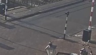
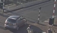
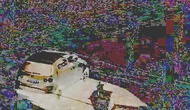
The second key technique in NoScope is the use of difference detectors: extremely efficient models that detect changes in labels. Given a labeled video frame (e.g. this frame does not have a car—a “false” in our binary classification setting) and an unlabeled frame, a difference detector determines whether the unlabeled frame has the same or different label compared to the labeled frame. Using these difference detectors, NoScope can quickly determine when video contents have changed. In videos where the frame rate is much higher than the label change rate (e.g., a 30 frame per second video capturing people walking across a 36 foot crosswalk), difference detectors can provide up to 90$\times$ speedups at inference time.

In general, the problem of determining label changes is as difficult as the binary classification task. However, as we have hinted above, videos contain a high degree of temporal locality, making the task of detecting redundant frames much easier. Figure 2 demonstrates this: subtracting a frame containing an empty scene from a frame containing a car distinctly highlights the car. In addition, since NoScope uses efficient difference detectors (i.e., much more efficient than even specialized models), only a small fraction of frames need to be filtered for difference detectors to be worth the cost of evaluation.

NoScope leverages two forms of difference detectors:

1. Difference detection against a fixed reference image for the video stream, that contains no objects. For example, for a video of a sidewalk, the reference image might be a frame of an empty sidewalk. NoScope computes the reference image by averaging frames where the reference model returns no labels.

2. Difference detection against an earlier frame a pre-configured time $t_{\mathrm{diff}}$ seconds into the past. In this case, if there are no significant differences, NoScope returns the same labels that it output for the previous frame. NoScope’s optimizer learns $t_{\mathrm{diff}}$ based on the input data.

The optimal choice of method is video-dependent, so NoScope’s optimizer performs selection automatically. For example, a video of a mostly empty sidewalk might have a natural empty reference image that one can cheaply and confidently compare with to skip many empty frames. In contrast, a video of a city park might always contain mobile objects (e.g., people lying down in the grass), but the objects might move slowly enough that comparing with frames 1 second ago can still eliminate many calls to the expensive reference model.

Given the two frames to compare, NoScope’s difference detector computes the Mean Square Error (MSE) between them as a measure of distance. NoScope either performs a comparison on the whole image, or a blocked comparison where it subdivides each image into a grid and computes the metric on every grid block. In the blocked version, NoScope then trains a logistic regression (LR) classifier to weigh each block when evaluating whether two images are different. The blocked version is more expensive to compute, but it is useful when part of the image does not contain relevant information. For example, in a street view, the signal will change colors frequently but this is not useful for detecting cars.

Using this distance metric, NoScope determines whether the frame contents have changed. The appropriate firing threshold for the metric, or the difference in metric at which we say that the two frames differ), which we will denote $\delta_{\mathrm{diff}}$, also depends on the video and the query. For example, a lower MSE threshold might be needed to detect light objects against a light background than dark ones.

We also considered alternative metrics including Normalized Root Mean Square Error, Peak Signal to Noise Ratio, and Sum of Absolute Differences. While different methods performed differently, MSE and blocked MSE were generally within a few percent of the best method, so NoScope currently only uses these two methods.

Finally, the difference detector has a configurable time interval $t_{\mathrm{skip}}$ that determines how often to perform a difference check. For example, objects of interest may appear in a scene for much longer than a second, so NoScope can test for differences every 15 frames in a 30 fps video. We refer to this behavior as frame skipping, and the frame skipping parameter directly creates a trade-off between accuracy and speed. Section 9.4 demonstrates that frame skipping is effective but is not responsible for all performance gains offered by NoScope.

As may be apparent, various configurations of the difference detector will give varying tradeoffs between execution speed, false positive rate and false negative rate depending on the video and query in question. NoScope’s optimizer, described below, selects and adjusts the difference detector automatically based on frames labeled using the expensive reference model to navigate this trade-off.

6 Cost-Based Model Search

NoScope combines model specialization and difference detectors using inference-optimized model search. NoScope uses a cost-based optimizer (CBO) to find a high-quality cascade of models (e.g., two vs four layer specialized model) and thresholds ($\delta_{\mathrm{diff}}$, $c_{\mathrm{low}}$, and $c_{\mathrm{high}}$). The CBO takes as input a video as well as target accuracy values, $\mathrm{FP}^{*}$ and $\mathrm{FN}^{*}$, for the false positive rate and false negative rate, respectively. Formally, the CBO solves the following problem:

$$\begin{array}[]{rl}\text{maximize}&E(\text{throughput})\\ \text{subject to}&\text{false positive rate}<\mathrm{FP}^{*}\\ \text{and}&\text{false negative rate}<\mathrm{FN}^{*}\end{array}$$

This problem is similar to traditional cost-based estimation for user-defined functions [21] and streaming filter processing [11, 9], but NoScope must also perform cost estimation of each candidate model and set model-specific parameters for each together to achieve a target accuracy goal. That is, NoScope’s problem is not simply a matter of ordering a set of commutative filters, but also requires searching the model architectures, learning the models, and setting their parameters together to achieve an overall end-to-end cascade accuracy.

To solve this problem, NoScope uses a combination of combinatorial search for model architectures and efficient linear sweeps for the firing thresholds $\delta_{\mathrm{diff}}$, $c_{\mathrm{low}}$, and $c_{\mathrm{high}}$. NoScope’s CBO only considers plans involving up to one difference detector and one specialized model because we found that stacking more such models did not help significantly. For such plans, the CBO can search the complete space of combinations of difference detectors and specialized models at a fraction of the cost of labeling all of the input video using a full NN such as YOLOv2. We now describe the key components of the CBO.

6.1 Training Data Generation

NoScope runs the full reference model on a subset of the video frames to generate labeled data. For example, NoScope could run the full NN over the first few days of a new stream, and maintain this set using reservoir sampling thereafter. Given this labeled data, NoScope’s CBO begins by splitting the input data into a training set and an evaluation set that will only be used for model selection.

6.2 Cost Model

To determine which combination of difference detector and specialized model to use, the CBO estimates the inference cost of each. NoScope models execution time per frame using the pass-through rates of the detector and specialized model in question on the training data, and static measurements of the execution time of each model on the target hardware. For example, consider a configuration with the following two filters:

1. A Mean Squared Error (MSE) difference detector that is configured to check frames every $t_{\mathrm{skip}}$ seconds and fire if the frame’s MSE with a reference image is higher than $\delta_{\mathrm{diff}}$.

2. A two-layer NN with 64 convolutional units and 64 neurons in the dense layer, with detection thresholds $c_{\mathrm{low}}$ and $c_{\mathrm{high}}$.

NoScope’s cost model determines the expected time per frame by first measuring what fraction of frames remain after the skipping done by $t_{\mathrm{skip}}$; call this fraction $f_{s}$. Next, it computes the fraction of these frames in the training data that pass the MSE filter, $f_{m}$. Finally, it computes the fraction of these difference detector passing frames whose confidence under the specialized NN lies between $c_{\mathrm{low}}$ and $c_{\mathrm{high}}$ – call this $f_{c}$. The selectivities ($f_{s}$, $f_{m}$, and $f_{c}$) are estimated from a sample of the data. The expected execution time per frame is then

$$f_{s}T_{\mathrm{MSE}}+f_{s}f_{m}T_{\mathrm{SpecializedNN}}+f_{s}f_{m}f_{c}T_{\mathrm{FullNN}}$$

where $T_{\mathrm{MSE}}$, $T_{\mathrm{SpecializedNN}}$ and $T_{\mathrm{FullNN}}$ are the execution times per frame for the MSE filter, specialized NN and reference NN respectively. These execution times are data-independent, so they can be measured once per hardware platform.

6.3 Model Search

Given input data and the above cost model, NoScope must find a suitable cascade. There are three main challenges in finding an optimal configuration. First, models may be complex and exhibit non-linearity with respect to the cascade architecture and input parameters: their selectivities will not be known a priori. Second, models are not independent (cf. [11]): one specialized model may complement one difference detector but not another, and the viable combinations of thresholds for each pair of models will differ across scenes. Third, the full search space for model configurations is very large because the firing thresholds $\delta_{\mathrm{diff}}$, $c_{\mathrm{low}}$ and $c_{\mathrm{high}}$ are continuous values.

NoScope addresses these challenges via a three-stage process. First, it trains each filter individually on our training set. Second, it examines each filter in isolation to determine the scores for each frame. Finally, it explores all combinations of difference detectors and specialized models and use an efficient linear sweep of the viable combinations of thresholds to determine the lowest-cost way to combine these models. In detail, NoScope’s search proceeds as follows:

1.) Train filters: First, NoScope trains each model (e.g., specialized NNs and LR based blocked difference detectors) on the training data. For the NNs, we consider a grid of combinations of model architectures (e.g., 2 or 4 layers, 32 or 64 convolutional units, etc). Currently, this is 24 distinct configurations. When training these models, NoScope subdivides the original training data to create a cross-validation set that is not part of training, for parameter selection.

2.) Profile individual filters: Next, NoScope performs selectivity estimation by profiling individual filters on its evaluation set (the input data that the CBO set aside at the beginning for evaluation) to determine their selectivity and sensitivity. These quantities are difficult to infer beforehand because they depend significantly on the video, so NoScope runs each trained model on every frame of the evaluation set. NoScope then logs the score that the filter gives to each frame (e.g., MSE or specialized NN output confidence), which it uses to set the thresholds $\delta_{\mathrm{diff}}$, $c_{\mathrm{low}}$ and $c_{\mathrm{high}}$.

3.) Examine filter combinations: Filter parameters are not independent because the thresholds for a pair of filters may influence one another and therefore need to be set together. For example, if NoScope uses MSE as our difference detection metric, the threshold $\delta_{\mathrm{diff}}$ that it sets for difference detection directly affects which frames are passed to the downstream specialized NN and which thresholds $c_{\mathrm{low}}$ and $c_{\mathrm{high}}$ it can set (e.g., if the difference detector induces many false negatives, the specialized model must be more conservative).

NoScope solves the problem of dependencies in filter selection via an efficient algorithm to sweep feasible combinations of thresholds. Specifically, for each difference detector $D$, NoScope first sorts the frames of the training data in decreasing order of the detector’s difference metric ($\delta$). This yields a list of frames $L_{D}$ where we can easily sweep through firing thresholds $\delta_{\mathrm{diff}}$. Next, for each prefix of the list $L_{D}$, NoScope computes the false positive and false negative rate for the given $\delta_{\mathrm{diff}}$ threshold (i.e., frames that we will mislabel due to the difference detector not firing).

Next, for each specialized NN, $C$, NoScope sorts the unfiltered frames by confidence. Given this list, we can set $c_{\mathrm{low}}$ and $c_{\mathrm{high}}$ to obtain the desired false positive and false negative rates $\mathrm{FP}^{*}$ and $\mathrm{FN}^{*}$: NoScope begins with thresholds at the extreme (0 and maximum confidence), then moves $c_{\mathrm{low}}$ up until the false negative rate of the combined difference detector and NN reaches $\mathrm{FN}^{*}$, and moves $c_{\mathrm{high}}$ down until the combined false positive rate reaches $\mathrm{FP}^{*}$. Finally, for each such combination of detector $D$, NN $C$, $\delta_{\mathrm{diff}}$, $c_{\mathrm{low}}$, and $c_{\mathrm{high}}$, NoScope computes the expected throughput using our cost model (Section 6.2) and outputs the best result. Note that because the CBO is only able to access training data, false positive and false negative rates are only guaranteed insofar as the training data reflects the testing data. Our experimental results demonstrate that this optimization strategy is sound for many real-world video feeds.

Running Time. The overall complexity of NoScope’s CBO is $O(n_{d}n_{c}n_{t})$, where $n_{d}$ is the total number of difference detector configurations considered, $n_{c}$ is the total number of specialized model configurations, and $n_{t}$ is the total number of firing thresholds considered during the sweep down $L_{D}$. In addition, we need to run each of the $n_{d}$ difference detectors and $n_{c}$ specialized model configurations on the training data once (but not each pair of filters together). Overall, the running time of the algorithm is often just a few seconds because each of $n_{d}$, $n_{c}$ and $n_{t}$ is small (less than 100). Even training and testing the specialized models we will test is faster than obtaining the “ground truth” labels for the training data using a full-scale NN like YOLOv2. As we show in Section 9.3.1, all steps of the CBO together run faster than labeling hours-long videos using a full NN.

7 Implementation

We implemented a NoScope prototype in C++ and TensorFlow (for the actual inference tasks), and Python (for the NoScope CBO). We optimized the code by parallelizing many of the CPU-intensive operations over multiple cores, using vectorized libraries, and batching data for computations on the GPU; we provide our code as open source. These optimizations make a large difference in performance for many configurations of NoScope because the bulk of the video frames are eliminated by the difference detector and specialized NN.

At a high level, given a video, NoScope performs the following four steps: 1) perform model search, 2) run the resulting difference detector, 3) run the resulting specialized NN on the frames that pass the difference detector, and 4) run the reference model such as YOLOv2 on the remaining frames that are not confidently labeled by the specialized model. We next describe each of these steps in turn.

Model Search Implementation. Our CBO is written in Python, and calls our C++ code for difference detectors and NNs when obtaining training data. As described in Section 6, the cost of the CBO itself is relatively small. The bulk of the runtime is spent training the specialized NN models on its input data.

We used YOLOv2 [80] as our reference model. We pre-load the YOLOv2 NN parameters onto the GPU and keep it in memory across evaluations to avoid reloading this large model both at optimization time and at inference time.

NoScope loads video frames either directly from memory or from OpenCV for video decoding. After loading frames, it resizes them for downstream processing if needed using OpenCV (our NNs require a specific size for input images, such as 416x416 pixels for YOLOv2).

Difference Detectors.

We implemented difference detectors in OpenCV and C++. For the MSE computation, we wrote hand-tuned C++ code to fuse together the required operations: MSE requires computing sum$\left((a-b)^{2}\right)$, where a and b are two images, which would require materializing a-b in memory using OpenCV’s standard array operators. Finally, we parallelized the difference detector at the level of frames—that is, we process multiple decoded frames in parallel using different threads.

We used scikit-learn to train the logistic regression weights for the blocked difference detectors that weigh different portions of the image differently. We then evaluate the resulting logistic regression models at runtime using C++ code.

Specialized Models. We train our specialized NNs using the TensorFlow framework. As discussed in Section 4, we used standard practices for NN training such as cross-validation and early stopping, and our CBO selects which NN to run using an evaluation set that is distinct from the training data.

During evaluation, we evaluate the specialized NNs on the GPU using TensorFlow’s C++ interface. We batch input images before passing them to the GPU due to the high cost of communication.

Finally, a key pre-processing step is to mean-center the pixel values and change the dynamic range in each color channel to [-1, 1]. We implemented this step on the CPU using OpenCV and multithreading in a similar manner to difference detection.

8 Limitations

While NoScope demonstrates significant promise in accelerating NN inference, we wish to highlight several important limitations:

Fixed-Angle Video. We designed the current prototype for the task of object classification in fixed-angle video (e.g., traffic cameras), which we believe represents an important subset of all video data processing. Therefore, our current difference detectors only work on video shot by static cameras, and our results for specialized CNNs are also obtained on fixed-angle videos. The video processing community has also developed techniques to track objects when the camera is moving [70], so these techniques present a promising approach to extend NoScope to moving cameras.

Binary Classification Task. We have only evaluated NoScope on the binary classification task; the techniques we present could already be used for more complex boolean queries. We believe the same techniques may apply elsewhere.

Model Drift. Our current implementation assumes that the training data obtained in NoScope’s optimizer is from the same distribution as the subsequent video observed. If the scene changes dramatically after a certain point of time, NoScope needs to be called again to re-optimize for the new data distribution. Likewise, if the scene changes periodically during the video (e.g., by cycling between day and night), the training data needs to contain frames representative of all conditions. We believe this is reasonable for many fixed-angle camera scenarios, such as traffic or security cameras, which observe a similar scene over a period of months or years. For these types of videos, a sample of training data spread throughout the year should be sufficient to produce good training data for a model that can be applied continuously. However, it would be interesting to address this limitation automatically (e.g., by tracking model drift).

Image Batching. Our implementation batches video frames for greater efficiency. While acceptable for historical video that is available all at once, batching can introduce a short delay for live video, proportional to the number of frames batched. For example, batching together 100 frames at a time in a 30 fps video can add a delay of 3.3 seconds. Alternatively, a system monitoring 100 streams might be able to batch together data from different streams, applying different NN models to each one, allowing a range of optimizations [69] we have not yet explored in the context of streaming video.

Table 1: Video streams and object labels queried in our evaluation.

Video Name	Object	Resolution	FPS	# Eval frames	Length (hrs)
taipei	bus	1000x570	30	1296k	12.0
coral	person	1280x720	30	1188k	11.0
amsterdam	car	680x420	30	1296k	12.0
night-street	car	1000x530	30	918k	8.5
store	person	1170x1080	30	559k	5.2
elevator	person	640x480	30	592k	5.5
roundabout	car	1280x720	25	731k	8.1

(a) coral without a person

(b) coral with a person

Figure 3: Example query, with and without the object of interest.

9 Evaluation

We evaluate NoScope on binary classification for real-world webcam and surveillance videos. We illustrate that:

1. NoScope achieves 40-5400$\times$ higher throughput (i.e. frames processed per second) than state-of-the-art NN models while maintaining 99% of their accuracy, and 100-10000$\times$ higher throughput while maintaining 90+% accuracy (§ 9.2).

2. The configuration of filters dramatically affects NoScope’s overall performance. Moreover, the optimal cascade for one video will almost always provide poor performance if used on another video (§ 9.3).

3. NoScope’s CBO consistently sets filter parameters that provide large performance improvements while maintaining specified accuracy. Difference detection and specialized models improve the throughput up to 3$\times$ and 340$\times$ respectively (§ 9.3).

4. Specializing models for a given video provides a 1.25-25$\times$ improvement over training models for the same detection task across multiple environments (§ 9.5).

5. NoScope’s outperforms both classical computer vision baselines as well as small, binary-classification NNs that are not specialized to a given video (§ 9.6).

9.1 Experimental Setup

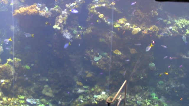
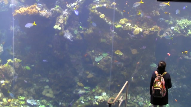
Evaluation Queries. We evaluate NoScope on a fixed set of queries depicted in Table 1. We use YOLOv2 [80], a state-of-the-art multi-scale NN, as our reference model. YOLOv2 operates on 416x416 pixel images (resizing larger or smaller images). YOLOv2 achieves 80 fps on the Tesla P100 GPU installed on our measurement machine. We obtain videos from seven webcams—six from YouTube Live, and one that we manually obtained. We split each video into two parts: training and evaluation. Five videos have two days worth of video, with 8-12 hours of footage per day due to lighting conditions; for these videos, we use the first day of video for training and the second day for evaluation. For two videos, we use the first 2.3 hours for training and separate an evaluation set (5-8 hours) by a minimum of 30 minutes. Figure 3 illustrates an example. By default, we set a target of 1% false positive and 1% false negative rates.

Evaluation Metrics. We measure throughput by timing the complete end-to-end system excluding the time taken to decode video frames. We omit video decode times for three reasons. First, it is standard to omit video decode time in computer vision [80, 79, 81]. Second, both GPUs and CPUs can decode video at a high rate because of built-in hardware decoders [75]. For example, our Tesla P100 can decode 400x400 H.264 video at 4000 fps and 400x400 MPEG video at 5600 fps with a single hardware decoder; some processors have multiple decoders. Third, for some visual sensors, we can directly obtain a raw stream of frames from the hardware.

We measure accuracy by comparing frames labeled by the reference model and NoScope in 30 frame windows. For a window to be considered labeled correctly, both systems must agree on the presence of the target object in 28 of the 30 frames in a window. We use this somewhat permissive accuracy measure because YOLOv2 often intermittently fails to label objects that are clearly visible in the frame.

Hardware Environment. We perform our experiments on an NVIDIA DGX-1 server, using at most one Tesla P100 GPU and 32 Intel Xeon E5-2698 v4 cores during each experiment. The complete system had 80 cores and multiple GPUs, but we limited our testing to a subset of these so our results would be representative of a less costly server. The system also had a total of 528 GB of RAM.

9.2 End-to-End Performance

(a) taipei

(b) coral

(c) amsterdam

(d) night-street

(e) store

(f) elevator

(g) roundabout

Figure 4: Accuracy vs. speedup achieved by NoScope on each dataset. Accuracy is the percent of correctly labeled time windows, and speedup is over YOLOv2. Note the y-axis starts at 80%.

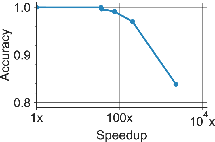
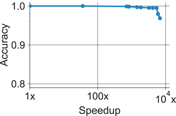
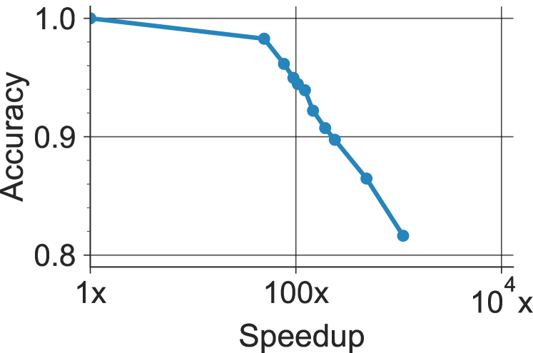
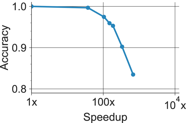
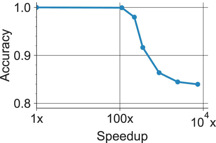
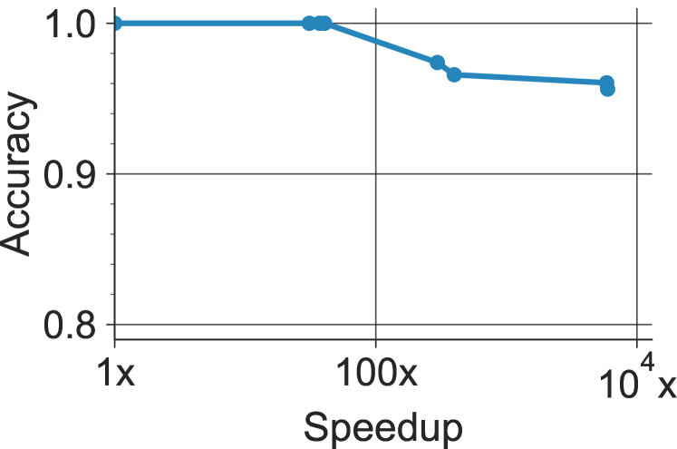
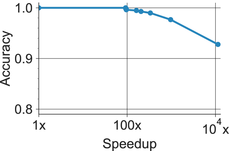
Figure 4 illustrates the overall range of performance that NoScope achieves on our target queries. For each dataset, we obtained the points in the plot by running NoScope’s CBO with increasing false positive and false negative thresholds ($\mathrm{FP}^{*}$ and $\mathrm{FN}^{*}$, with $\mathrm{FP}^{*}=\mathrm{FN}^{*}$) and measuring the resulting speedup. NoScope demonstrates several orders of magnitude speedup across all the datasets, with magnitude depending on the desired accuracy levels. In all cases, NoScope achieves a 30$\times$ speedup with at least 98% accuracy. In many cases, this level of accuracy is retained even at a 100$\times$ speedup, and NoScope can obtain 1000$\times$ to 10,000$\times$ speedups at 90+% accuracy. The video with the lowest peak speedup at the 90% accuracy mark is taipei, which shows a busy intersection—thus, the difference detectors cannot eliminate many frames. However, even in this video, NoScope can offer an 30$\times$ speedup over YOLOv2 with no loss in accuracy.

Table 2: Filter types and thresholds chosen by NoScope’s CBO for each video at 1% target false positive and false negative rates. Both the filter types (e.g., global or blocked MSE) and their thresholds (e.g., the difference in MSE that is considered significant, or the upper and lower detection thresholds for the specialized models) vary significantly across videos. For the specialized models (denoted SM), L denotes the number of layers, C the number of convolutional units, and D the dimension of the dense layers.

Video Name	DD	$\delta_{\mathrm{diff}}$	SM (L)	SM (C)	SM (D)	$c_{\mathrm{low}}$	$c_{\mathrm{high}}$
taipei	global	37.5	2	64	32	0.114	0.994
coral	blocked	147.3	2	16	128	0.0061	0.998
amsterdam	global	0.0019	2	64	256	0.128	0.998
night-street	global	0.441	2	16	128	2.2e-7	0.176
store	blocked	336.7	2	32	128	0.010	0.998
elevator	global	0.0383	2	32	256	0.004	0.517
roundabout	global	0.115	4	32	32	0.0741	0.855

9.3 Impact of the CBO

To better understand the source of speedups, we explored the impact of NoScope’s CBO on performance. We begin by showing that the filter types and thresholds chosen by the CBO differ significantly across videos based on the characteristics of their contents. We also show that choosing other settings for these parameters would greatly decrease speed or accuracy in many cases, so parameters cannot be transferred across videos.

Configurations Chosen Across Datasets. Table 2 shows the difference detectors, specialized models, and detection thresholds chosen by the CBO across our sample datasets for a 1% target false positive and false negative rate. We observe that these are substantially different across videos, even when the CBO selects the same filter class (e.g., difference detection based on global MSE). We make a few observations about these results:

First, the best type of MSE chosen depend on the video. For example, coral and store are scenes with a dynamic background (e.g., coral shows an aquarium with colorful fish swimming in the background, and NoScope is asked to detect people in the scene). In these scenes, computing MSE against several frames past instead of against a single “empty” reference frame is more effective.

Second, the chosen thresholds also differ significantly. For example, taipei has a high difference detection threshold due to high levels of small-scale activity in the background, but the target objects, buses, are generally large and change more of the frame. The upper and lower thresholds for NNs also vary even across the same target object class, partly due to varying difficulty in detecting the objects in different scenes. For example, in some videos, the $c_{\mathrm{low}}$ threshold for declaring that there is no object in a frame is extremely low because increasing it would lead to too many false negatives.

Third, the best specialized model architectures also varied by video and query. In particular, we found that in many videos, the larger NNs (with 4 layers or with more convolutional units and dense layer neurons) would overfit given the fairly small training set we used (150,000 frames out of the 250,000 frames set aside for both training and evaluation). However, the best combination of the model architecture parameters varied across videos, and NoScope’s training routine that selects models based on an unseen evaluation set automatically chose an accurate model that did not overfit.

Non-Transferability Across Datasets. As the best filter configurations varied significantly across datasets, transferring parameters from one dataset to another leads to poor performance:

Figure 5: Normalized performance of NoScope with two different specialized NN models on the night-street and taipei videos. We see that choosing a different NN architecture for each video, even though this architecture performed well on another dataset, reduces throughput. NoScope automatically selects the best-performing NN.

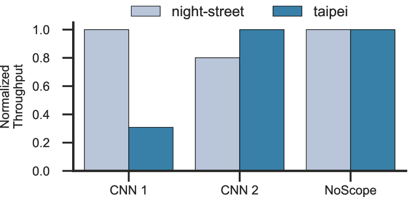
Specialized Model Architectures. We used the specialized model architecture from night-street (a NN with parameters L=2, C=16, D=128) on the taipei dataset (whose optimal NN had L=2, C=64, D=32), and vice-versa. We transferred only the architecture, not the learned model from each dataset and trained a new model with each architecture for the new dataset to evaluate its performance there. Although these architectures have similar properties (e.g., two layers), they required significantly different parameters to achieve our 1% target false positive and false negative rates on each dataset. This resulted in a 1.25$\times$ to 3$\times$ reduction in throughput for the overall NoScope pipeline, as depicted in Figure 5.

Figure 6: Firing thresholds $\delta_{\mathrm{diff}}$ chosen by the CBO for each video (blue dots), along with the range of thresholds that can achieve 1% false positive and false negative rate for that video (black lines).

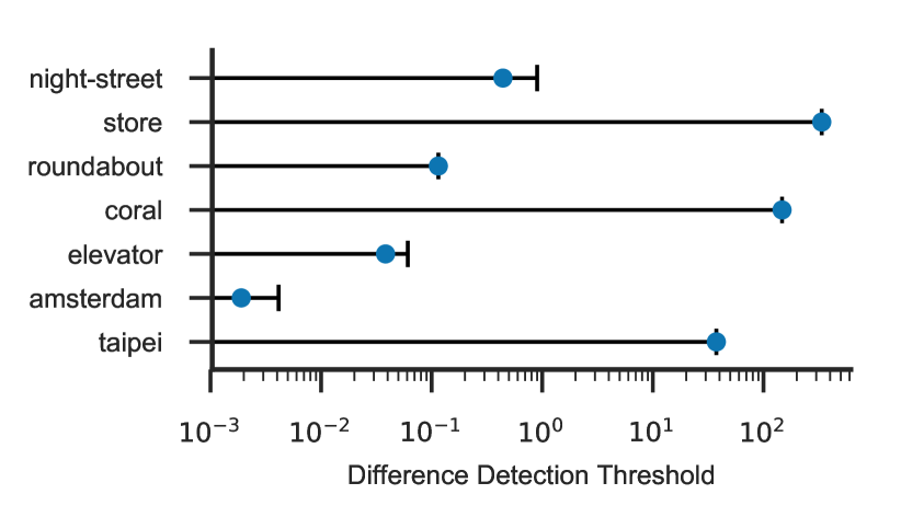
Detection Thresholds. We plotted the range of feasible thresholds for the difference detector ($\delta_{\mathrm{diff}}$), as well as the actual threshold chosen, in Figure 6. Feasible thresholds here are the ones where the system can stay within the 1% false positive and false negative rates we had requested for the CBO. Beyond a certain upper limit, the difference detector alone will introduce too many incorrect labels (on the validation set). As we see in the plot, the range of values for each video is different and the best-performing threshold is often near the top of this range, but not always. For example, coral is near the top, but amsterdam is lower, this is due to the downstream performance of the specialized models. Thus, attempting to use a common threshold between videos would either result in failing to achieve the accuracy target (if the threshold is too high) or lower performance than the threshold NoScope chose (if the threshold is too low).

9.3.1 Running Time of the CBO

Figure 7: Breakdown of training and optimization time on taipei dataset. Passing all the training frames through YOLOv2 to obtain their true labels dominates the cost, followed by training all variants of our specialized models and then the rest of the steps in the CBO.

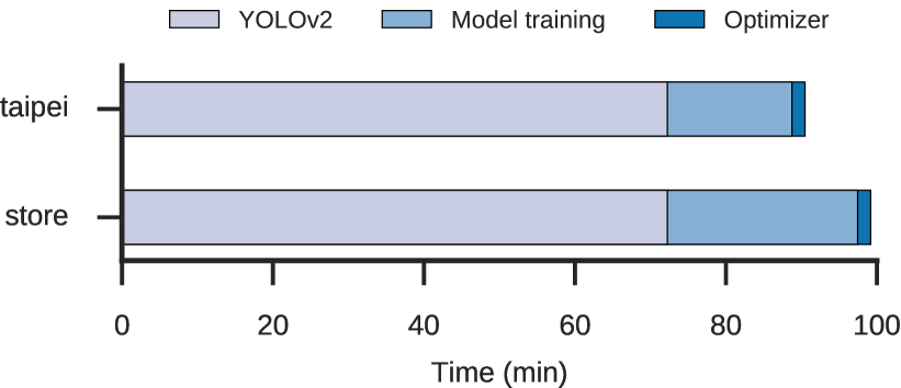
We measured the time it takes to run our CBO across several datasets, showing the most time-consuming one in Figure 7. In all cases, initializing NoScope requires labeling all the frames in the training data with YOLOv2, followed by training all supported specialized models and difference detectors on this data, then selecting a combination of them using the algorithm in Section 6. The CBO is efficient in the number of samples required: only 250k samples are required to train the individual filters and set the thresholds. For the longer videos, we randomly sample from the training set and for the shorter videos we use the first 250k frames. As shown in the figure, YOLOv2 application takes longer than all the other steps combined, meaning that NoScope’s CBO could run in real time on a second GPU while the system is first observing a new stream. Training of the specialized NNs takes the next longest amount of time; in this case, we trained 24 different model architectures. We have not yet optimized this step or tried to reduce the search space of models, so it may be possible to improve it.

9.4 Impact of Individual Models

(a) Factor analysis

(b) Lesion study

Figure 8: Factor analysis and lesion study of NoScope’s filters. The factor analysis shows the impact of adding different filters for two videos; from left to right, we add each of the filters in turn over YOLOv2. The lesion study shows the impact of removing filters; the leftmost bars show normalized performance with all of NoScope’s features enabled, and the remaining bars to the right show the effect of removing each filter from NoScope. (Note the logarithmic scale on the y-axes of both plots.)

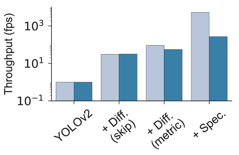
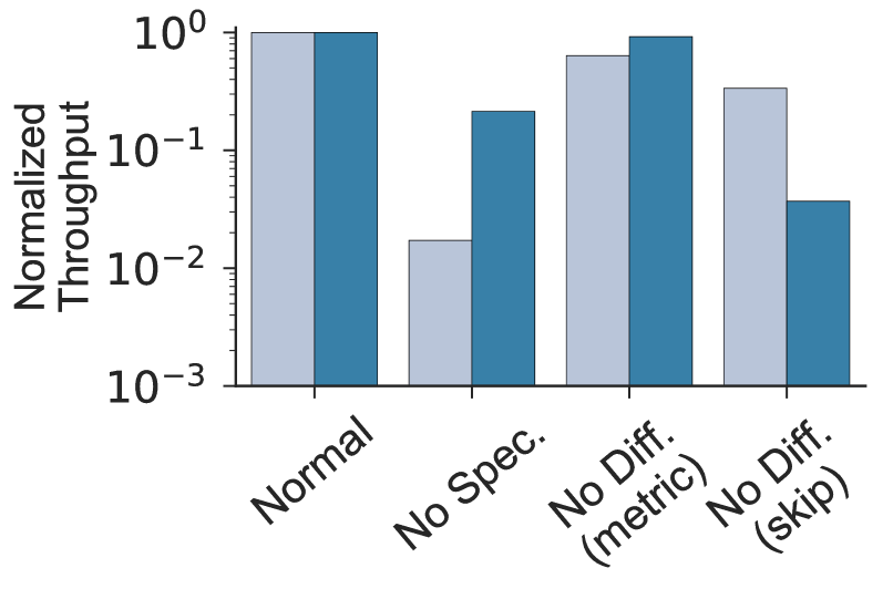
To analyze the impact of each of our model types on NoScope’s performance, we ran a factor analysis and lesion study on two videos, with results shown in Figures 8(a) and 8(b).

In the factor analysis, we started by running all frames through YOLOv2 and gradually added: difference detection’s frame skipping, difference detection on the skipped frames, and specialized model evaluation. Each filter adds a nontrivial speedup: skipping contributes up to 30$\times$, content-based difference detection contributes up to 3$\times$, and specialized models contribute up to 340$\times$.

In the lesion study, we remove one element at a time from the complete NoScope cascade. As shown in Figure 8(b), each element contributes to the overall throughput of the pipeline, showing that each component of NoScope’s cascades are important to its performance.

9.5 Impact of Model Specialization

Figure 9: Throughput, Generic NN vs. NoScope. Substituting the specialized NN model in NoScope with an equivalent model trained on MS-COCO (a general-purpose training set of images used by YOLOv2) results in a decrease in the end-to-end throughput of the system across all videos.

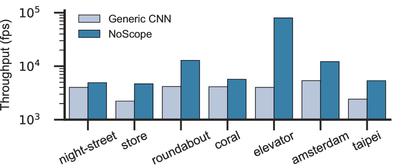
Finally, we evaluate the benefit of video-specific model specialization compared to training on general computer vision datasets. Our hypothesis in designing NoScope was that we can achieve much higher accuracy by training models on past frames from the same video to leverage the characteristics of that particular scene (e.g., fixed perspective on the target object, fixed background, etc.). To evaluate this hypothesis, we trained three deep NNs for binary classification on the classes of objects we evaluate NoScope on: people, buses, and cars using the more general MS-COCO dataset [62], a recent high-quality object detection dataset. For each class, we selected the best model from the same model family as NoScope’s CBO. Figure 9 shows the resulting throughput across our videos. In all cases, the specialized models trained by NoScope outperform the generic model of the same size trained on MS-COCO (up to 20$\times$), showing that scene-specific specialization has a significant impact on designing models for efficient inference.

9.6 Comparison Against Baselines

Figure 10: Comparison against classical and NN baselines. Experiments are run on elevator with frame skipping enabled for all models.

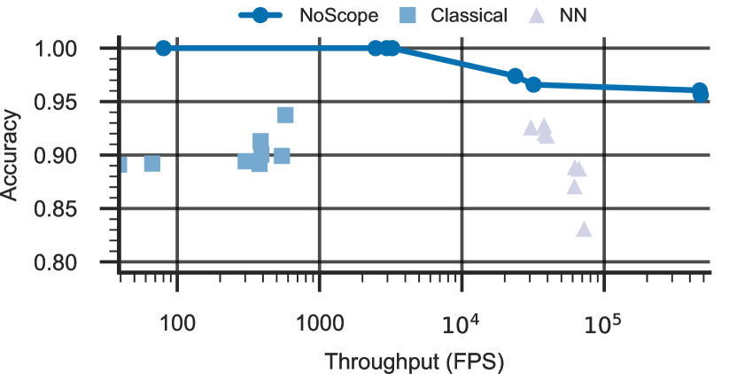
We also compared to classic methods in computer vision, including a deformable parts model (which performed favorably in the ImageNet 2012 [82]), a variety of SIFT-based bag-of-words classifiers (varying the SIFT parameters), and selective search with a SIFT-based classifier [63] (which performed well on PASCAL VOC [32]). We use implementations from OpenCV, a reference standard optimized computer vision library. Additionally, we trained several classification deep networks on the MS-COCO [62] dataset, varying hyper-parameters (2-10 convolutional layers and 1-2 fully connected layers). Figure 10 illustrates the resulting accuracy-speedup trade-offs for these models combined with frame skipping. NoScope is nearly a thousand times faster than several classical baselines while achieving higher accuracy. Additionally, non-specialized deep networks also fail to achieve comparable accuracy. Thus, specialization is key to accurate and efficient inference, and NoScope provides a means of smoothly trading accuracy for speed.

10 Related Work

NoScope builds on a long tradition of data management for multimedia and video and upon recent advances in computer vision, machine learning, and computer architecture. We outline several major related thrusts below.

Visual Data Management. Data management researchers have long recognized the potential of computer vision techniques for organizing and querying visual data—starting with early systems such as Chabot [72] and QBIC [36], and followed by a range of “multimedia” databases for storing [7, 59], querying [101, 73, 6, 57], and managing [38, 48, 94] video data. Similar techniques are deployed in commercial software such as Oracle Multimedia and Google Image Search. Many of these systems use classic computer vision techniques such as low-level image features (e.g., colors, textures), and many of them rely on augmenting video with text for richer semantic queries; however, with the advent of neural networks, we believe it is worthwhile to revisit many of these system architectures.

Computer Vision Tasks. In the design of its CBO and model cascade, NoScope draws on a range of computer vision techniques:

Model Cascades. The concept of combining a sequence of classifiers to improve inference speed is known as a cascade. One of the first cascades, the Viola-Jones detector [90], cascades traditional image processing features; if any classifier is confident about the output, the Viola-Jones cascade short-circuits evaluation, improving execution speed. Recent work has focused on learning cascades for pedestrian detection [18] and facial recognition [85, 60] image tasks. In NoScope, we design a cascade architecture for use in video, specifically adapted to account for temporal locality (via difference detectors) and query simplicity (via model specialization). Similar to NoScope, several NNs specialized for video take multiple frames as input to improve accuracy [91, 33], but again, these NNs focus on accuracy, not inference speed. Finally, NoScope’s use of a cost-based optimizer to optimize the end-to-end cascade (i.e., selecting different filters and choosing different thresholds for each filter based on the video stream and a reference NN) is novel compared to work in the computer vision literature that uses the same cascade of filters (or that optimize solely for accuracy, not computational cost; cf. [89]). In this way, NoScope acts as a system for model search [14, 23, 102] for efficient inference and is inspired by conventional database cost optimization [83] and related efforts on self-adapting query processing engines [47, 20].

Video Object Detection/Extraction and Tracking. The overall task of object detection and extraction is a core task in computer vision. As we have discussed, the explosion of recent interest in deep networks for this task have largely focused on improving accuracy. Object detection in video is becoming increasingly popular: since 2015, the ImageNet competition has had a video detection task [82]. State-of-the-art methods [50, 51, 43] follow a common pattern: run still image detection over every frame of the video and post-process the result. As still image detection is a building block of these methods, they are not optimized to exploit forms of temporal locality and instead primarily focus on accuracy; in contrast, NoScope focuses on the trade-off between accuracy and inference speed.

Beyond object detection, object tracking refers to the task of tracking an object through a video and is a vital tool in video analysis [93]. There are many such methods for tracking, including NN-based methods [71, 24] and traditional methods [27, 30], that all performed well on the VOT2016 challenge [55]. In a recent survey of object tracking methods, the fastest method runs at only 3.2k fps [92], and the above methods run much slower. NoScope solves the simpler task of binary classification, and we see extending NoScope to detection as a valuable area for future work.

Video Monitoring. Video monitoring captures a variety of tasks [52], ranging from object detection [53] to vehicle tracking [87]. Historically, these systems have been tailored to a specific task (e.g. license plate detection [5], counting cars [97], tracking pedestrians or cars [10]). Our goal in this work is to provide an automatic and generic framework for tailoring reference NNs to new tasks.

Scene Change Detection. NoScope leverages difference detectors to determine when labels for video contents have likely changed. This task is closely related to the task of scene change detection, in which computer vision techniques highlight substantial changes in video (e.g., cuts or fades in movies) [49, 16]. NoScope’s use of difference detection is inspired by these techniques but differs in two critical respects. First, NoScope’s difference detectors highlight changes in label (e.g., bus enters), not just changes in scene. Second, NoScope works over fixed-angle cameras. We expect many of these prior techniques to be useful in adapting NoScope to moving cameras.

Image Retrieval. Image retrieval is closely related to image classification. Retrieval typically takes one of two forms. The first is to associate images with a specific object or place of interest (e.g., this image is a photograph of a specific building on Stanford’s campus [76]). This first class of techniques are not directly applicable to our target setting: for example, in the night-street query, our task is to identify the presence of any car, not a specific car. The second class of techniques allows retrieval of similar images from a large corpus that are similar to a query image [61, 96] (e.g., Google Reverse Image search). One could use retrieval techniques such as k-nearest neighbors to perform binary classification. However, in this work, we leverage state of the art models—i.e., deep neural networks—that are specifically trained for the binary classification task.

Improving Deep Network Speed. Two recent directions in related work study the problem of accelerating deep network inference time:

Model Compression and Distillation. Model compression/distillation, i.e. producing a smaller, equivalent model from a larger model, has been proposed to reduce the size and evaluation time of NNs. One strategy for model compression is to use the behavior of a larger model (e.g., its output confidences) to train a smaller model, either distilling an ensemble of models into a smaller model [17], or distilling one large network into one smaller network [45, 8]. Another strategy is to modify the network weights directly, either via hashing [22] or pruning and literal compression of the weights themselves [41, 77]. These networks are almost always more amenable to hardware acceleration—a related line of research [42, 78]. The key difference between this related work and our model specialization method is that this related work is designed to produce smaller models preserve the full generality of the large model: that is, the small model can perform all of the tasks as the large model, without any loss in accuracy. In contrast, NoScope explicitly specializes NNs that were trained on a large variety of input images and target objects to instead operate over a specific video with a smaller number of target objects; this specialization is key to improving performance.

Model Specialization. We are not aware of any other work accelerating NN inference time via task specialization on video. However, related strategies for specialization have been shown to boost accuracy (but not runtime) [68, 65], and there are a range of models designed for detecting specific classes of objects in video. One of the most popular video-based object detection tasks is pedestrian detection [28, 15], with a range of NN-based approaches (e.g., [84]). In NoScope, our goal is to specialize to a range of inputs automatically, using a large general NN as guidance. We evaluate a handful of different labels based on available datasets, but theoretically any class recognized by NNs today could be specialized.

ML Model Management and Stream Processing Systems. While we have provided an overview of related multimedia query engines and a comparison with several filter- and UDF-based query processors in Section 6, NoScope also draws inspiration from a number of recent machine learning model management systems. Velox [25] provides a high-performance platform for serving personalized models at scale, while MLBase [54] provides a declarative interface for specifying modeling tasks, and MacroBase [13, 12] provides a platform for executing classification and data aggregation tasks on fast data. Similarly, a range of systems from academia and industry provide stream processing functionality [4, 19, 26, 39]; here, we specifically focus on video stream processing. Like Bismarck [35], NoScope is structured as a sequence of dataflow operators, but for performing video classification. Of these systems, MacroBase is the most closely related; however, in NoScope, we focus specifically on video classification and develop new operators and a CBO for that task. Looking forward, we are eager to integrate NoScope’s classifiers into MacroBase and similar systems.

11 Conclusions

Video is one of the richest and most abundant sources of data available. At the same time, neural networks (NNs) have dramatically improved our ability to extract semantic information from video. However, naïvely applying NNs to detect objects in video is prohibitively expensive at scale, currently requiring a dedicated GPU to run at real-time. In response, we presented NoScope, a system for accelerating inference over video at scale by up to three orders of magnitude via inference-optimized model search. NoScope leverages two types of models: specialized models that forego the generality of standard NNs in exchange for much faster inference, and difference detectors that identify temporal differences across frames. NoScope combines these model families in a cascade by performing efficient cost-based optimization to select both model architectures (e.g., number of layers) and thresholds for each model, thus maximizing throughput subject to a specified accuracy target. Our NoScope prototype demonstrates speedups of two- to three orders of magnitude for binary classification on fixed-angle video streams, with 1-5% loss in accuracy. These results suggest that by prioritizing inference time in model architecture search, state-of-the-art NNs can be applied to large datasets with orders of magnitude lower computational cost.

References

- [1] Typical cnn architecture. Creative Commons Attribution-Share Alike 4.0 International, Wikimedia Commons.
- [2] Cisco VNI forecast and methodology, 2015-2020. Technical report, 2016.
- [3] 2017. https://fortunelords.com/youtube-statistics/.
- [4] D. J. Abadi et al. The design of the Borealis stream processing engine. In CIDR, 2005.
- [5] C.-N. E. Anagnostopoulos et al. License plate recognition from still images and video sequences: A survey. IEEE Trans. on intelligent transportation systems, 2008.
- [6] W. Aref et al. Video query processing in the VDBMS testbed for video database research. In ACM-MMDB, 2003.
- [7] F. Arman et al. Image processing on compressed data for large video databases. In ACMMM, 1993.
- [8] J. Ba and R. Caruana. Do deep nets really need to be deep? In NIPS, 2014.
- [9] B. Babcock et al. Operator scheduling in data stream systems. VLDBJ, 2004.
- [10] B. Babenko et al. Robust object tracking with online multiple instance learning. IEEE trans. on pattern analysis and machine intelligence, 2011.
- [11] S. Babu et al. Adaptive ordering of pipelined stream filters. In SIGMOD, 2004.
- [12] P. Bailis et al. Macrobase: Prioritizing attention in fast data. In SIGMOD, 2017.
- [13] P. Bailis, E. Gan, K. Rong, and S. Suri. Prioritizing attention in fast data: Principles and promise. In CIDR, 2017.
- [14] M. G. Bello. Enhanced training algorithms, and integrated training/architecture selection for multilayer perceptron networks. IEEE Trans. on Neural networks.
- [15] R. Benenson et al. Ten years of pedestrian detection, what have we learned? In ECCV, 2014.
- [16] R. Brunelli, O. Mich, and C. M. Modena. A survey on the automatic indexing of video data. Journal of visual communication and image representation, 1999.
- [17] C. Bucilua et al. Model compression. In KDD, 2006.
- [18] Z. Cai et al. Learning complexity-aware cascades for deep pedestrian detection. In ICCV, 2015.
- [19] S. Chandrasekaran et al. TelegraphCQ: Continuous dataflow processing for an uncertain world. In CIDR, 2003.
- [20] S. Chaudhuri and V. Narasayya. Self-tuning database systems: a decade of progress. In VLDB, 2007.
- [21] S. Chaudhuri and K. Shim. Optimization of queries with user-defined predicates. TODS, 24(2):177–228, 1999.
- [22] W. Chen et al. Compressing neural networks with the hashing trick. In ICML, 2015.
- [23] Y. Cheng et al. An exploration of parameter redundancy in deep networks with circulant projections. In ICCV, 2015.
- [24] Z. Chi et al. Dual deep network for visual tracking. IEEE Trans. on Image Processing, 2017.
- [25] D. Crankshaw et al. The missing piece in complex analytics: Low latency, scalable model management and serving with Velox, 2015.
- [26] C. Cranor et al. Gigascope: a stream database for network applications. In SIGMOD, 2003.
- [27] M. Danelljan et al. Beyond correlation filters: Learning continuous convolution operators for visual tracking. In ECCV, 2016.
- [28] P. Dollar et al. Pedestrian detection: An evaluation of the state of the art. TPAMI, 34(4):743–761, 2012.
- [29] J. Donahue et al. Long-term recurrent convolutional networks for visual recognition and description. In CVPR, 2015.
- [30] D. Du et al. Online deformable object tracking based on structure-aware hyper-graph. IEEE Trans. on Image Processing, 2016.
- [31] A. Esteva et al. Dermatologist-level classification of skin cancer with deep neural networks. Nature, 542(7639):115–118, 2017.
- [32] M. Everingham et al. The PASCAL Visual Object Classes Challenge 2012 (VOC2012) Results.
- [33] C. Feichtenhofer et al. Spatiotemporal residual networks for video action recognition. In NIPS, 2016.
- [34] P. F. Felzenszwalb et al. Object detection with discriminatively trained part-based models. IEEE TPAMI, 2010.
- [35] X. Feng et al. Towards a unified architecture for in-RDBMS analytics. In SIGMOD, 2012.
- [36] M. Flickner et al. Query by image and video content: The QBIC system. Computer, 1995.
- [37] A. Geiger, P. Lenz, and R. Urtasun. Are we ready for autonomous driving? the kitti vision benchmark suite. In CVPR, 2012.
- [38] S. Gibbs et al. Audio/video databases: An object-oriented approach. In ICDE, 1993.
- [39] L. Girod et al. Wavescope: a signal-oriented data stream management system. In ICDE, 2006.
- [40] I. Goodfellow, Y. Bengio, and A. Courville. Deep Learning. MIT Press, 2016.
- [41] S. Han et al. Deep compression: Compressing deep neural networks with pruning, trained quantization and huffman coding. In ICLR, 2016.
- [42] S. Han et al. EIE: efficient inference engine on compressed deep neural network. In ISCA, 2016.
- [43] W. Han et al. Seq-nms for video object detection. CoRR, abs/1602.08465, 2016.
- [44] K. He et al. Deep residual learning for image recognition. In CVPR, 2016.
- [45] G. Hinton et al. Distilling the knowledge in a neural network. NIPS, 2014.
- [46] G. Hinton and T. Tieleman. Lecture 6.5 - rmsprop. Technical report, 2012.
- [47] S. Idreos, M. L. Kersten, S. Manegold, et al. Database cracking. In CIDR, 2007.
- [48] R. Jain and A. Hampapur. Metadata in video databases. In SIGMOD, 1994.
- [49] H. Jiang et al. Scene change detection techniques for video database systems. Multimedia systems, 1998.
- [50] K. Kang et al. Object detection from video tubelets with convolutional neural networks. In CVPR, pages 817–825, 2016.
- [51] K. Kang et al. T-cnn: Tubelets with convolutional neural networks for object detection from videos. arXiv preprint arXiv:1604.02532, 2016.
- [52] V. Kastrinaki, M. Zervakis, and K. Kalaitzakis. A survey of video processing techniques for traffic applications. Image and vision computing, 2003.
- [53] J. B. Kim and H. J. Kim. Efficient region-based motion segmentation for a video monitoring system. Pattern Recognition Letters, 24(1):113–128, 2003.
- [54] T. Kraska et al. Mlbase: A distributed machine-learning system. In CIDR, 2013.
- [55] M. Kristan et al. The visual object tracking vot2016 challenge results. ECCV, 2016.
- [56] A. Krizhevsky et al. Imagenet classification with deep convolutional neural networks. In NIPS, 2012.
- [57] M. La Cascia and E. Ardizzone. Jacob: Just a content-based query system for video databases. In ICASSP, 1996.
- [58] Y. LeCun et al. Deep learning. Nature, 521(7553):436–444, 2015.
- [59] J. Lee, J. Oh, and S. Hwang. Strg-index: Spatio-temporal region graph indexing for large video databases. In SIGMOD, 2005.
- [60] H. Li et al. A conv. neural network cascade for face detection. In CVPR, 2015.
- [61] K. Lin et al. Deep learning of binary hash codes for fast image retrieval. In CVPR, 2015.
- [62] T.-Y. Lin et al. Microsoft coco: Common objects in context. September 2014.
- [63] D. G. Lowe. Object recognition from local scale-invariant features. In ICCV, 1999.
- [64] D. Lu and Q. Weng. A survey of image classification methods and techniques for improving classification performance. International journal of Remote sensing, 28(5):823–870, 2007.
- [65] H. Maâmatou et al. Sequential Monte Carlo filter based on multiple strategies for a scene specialization classifier. EURASIP Journal on Image and Video Processing, 2016.
- [66] J. Malik. Technical perspective: What led computer vision to deep learning? Communications of the ACM, 60(6):82–83, 2017.
- [67] C. Metz. AI is about to learn more like humans—with a little uncertainty. Wired, 2017. https://goo.gl/yCvSSz.
- [68] A. Mhalla et al. Faster R-CNN scene specialization with a sequential Monte-Carlo framework. In DICTA, 2016.
- [69] K. Munagala et al. Optimization of continuous queries with shared expensive filters. In SIGMOD, 2007.
- [70] D. Murray and A. Basu. Motion tracking with an active camera. IEEE Trans. Pattern Anal. Mach. Intell., 16(5):449–459, May 1994.
- [71] H. Nam et al. Modeling and propagating cnns in a tree structure for visual tracking. arXiv:1608.07242, 2016.
- [72] V. E. Ogle and M. Stonebraker. Chabot: Retrieval from a relational database of images. Computer, 28(9):40–48, 1995.
- [73] J. Oh and K. A. Hua. Efficient and cost-effective techniques for browsing and indexing large video databases. In SIGMOD, 2000.
- [74] S. A. Papert. The summer vision project. 1966.
- [75] A. Patait and E. Young. High performance video encoding with NVIDIA GPUs. 2016 GPU Technology Conference (https://goo.gl/Bdjdgm), 2016.
- [76] J. Philbin et al. Object retrieval with large vocabularies and fast spatial matching. In CVPR, pages 1–8. IEEE, 2007.
- [77] M. Rastegari et al. Xnor-net: Imagenet classification using binary convolutional neural networks. In ECCV, 2016.
- [78] B. Reagen et al. Minerva: Enabling low-power, highly-accurate deep neural network accelerators. In ISCA, 2016.
- [79] J. Redmon et al. You only look once: Unified, real-time object detection. CVPR, 2016.
- [80] J. Redmon and A. Farhadi. Yolo9000: Better, faster, stronger. arXiv preprint arXiv:1612.08242, 2016.
- [81] S. Ren et al. Faster r-cnn: Towards real-time object detection with region proposal networks. In NIPS, 2015.
- [82] O. Russakovsky et al. Imagenet large scale visual recognition challenge. IJCV, 2015. http://image-net.org/.
- [83] P. G. Selinger et al. Access path selection in a relational database management system. In SIGMOD, 1979.
- [84] P. Sermanet et al. Pedestrian detection with unsupervised multi-stage feature learning. In CVPR, 2013.
- [85] Y. Sun et al. Deep conv. network cascade for facial point detection. In CVPR, 2013.
- [86] R. Szeliski. Computer vision: algorithms and applications. Springer Science & Business Media, 2010.
- [87] B. Tian, Q. Yao, Y. Gu, K. Wang, and Y. Li. Video processing techniques for traffic flow monitoring: A survey. IEEE, 2011.
- [88] J. R. Uijlings et al. Selective search for object recognition. IJCV, 2013.
- [89] R. Verschae et al. A unified learning framework for object detection and classification using nested cascades of boosted classifiers. Machine Vision and Applications, 19(2), 2008.
- [90] P. Viola and M. Jones. Rapid object detection using a boosted cascade of simple features. In CVPR, 2001.
- [91] P. Weinzaepfel et al. Learning to track for spatio-temporal action localization. In ICCV, 2015.
- [92] Y. Wu, J. Lim, and M.-H. Yang. Online object tracking: A benchmark. In CVPR, pages 2411–2418, 2013.
- [93] A. Yilmaz et al. Object tracking: A survey. CSUR, 2006.
- [94] A. Yoshitaka and T. Ichikawa. A survey on content-based retrieval for multimedia databases. TKDE, 11(1):81–93, 1999.
- [95] K.-H. Yu et al. Predicting non-small cell lung cancer prognosis by fully automated microscopic pathology image features. Nature Comm., 2016.
- [96] J. Yue-Hei Ng, F. Yang, and L. S. Davis. Exploiting local features from deep networks for image retrieval. In CVPR, pages 53–61, 2015.
- [97] H. Zhang et al. Live video analytics at scale with approximation and delay-tolerance. NSDI, 2017.
- [98] S. Zhang et al. How far are we from solving pedestrian detection? In CVPR, 2016.
- [99] W. Zhao et al. Face recognition: A literature survey. CSUR, 2003.
- [100] Q. Zhu et al. Fast human detection using a cascade of histograms of oriented gradients. In CVPR. IEEE, 2006.
- [101] X. Zhu et al. Video data mining: Semantic indexing and event detection from the association perspective. TKDE, 17(5):665–677, 2005.
- [102] B. Zoph and Q. V. Le. Neural architecture search with reinforcement learning. In ICLR, 2017.