Faster Coordinate Descent via Adaptive Importance Sampling


Dmytro Perekrestenko                        Volkan Cevher                        Martin Jaggi

ETH Zurich                        EPFL                        EPFL

Abstract

Coordinate descent methods employ random partial updates of decision variables in order to solve huge-scale convex optimization problems. In this work, we introduce new adaptive rules for the random selection of their updates. By adaptive, we mean that our selection rules are based on the dual residual or the primal-dual gap estimates and can change at each iteration. We theoretically characterize the performance of our selection rules and demonstrate improvements over the state-of-the-art, and extend our theory and algorithms to general convex objectives. Numerical evidence with hinge-loss support vector machines and Lasso confirm that the practice follows the theory.

1 Introduction

Coordinate descent methods rely on random partial updates of decision variables for scalability. Indeed, due to their space and computational efficiency as well as their ease of implementation, these methods are the state-of-the-art for a wide selection of standard machine learning and signal processing applications (Fu, 1998; Hsieh et al., 2008; Wright, 2015).

Basic coordinate descent methods sample an active coordinate set for optimization uniformly at random, cf., Stochastic Dual Coordinate Ascent (SDCA) Shalev-Shwartz and Zhang (2013) and other variants Friedman et al. (2007, 2010); Shalev-Shwartz and Tewari (2011). However, recent results suggest that by employing an appropriately defined non-uniform fixed sampling strategy, the convergence can be improved both in the theory as well as in practice Zhao and Zhang (2014); Necorara et al. (2012); Nesterov (2012).

In this work, we show that we can surpass the existing convergence rates by exploiting adaptive sampling strategies that change the sampling probability distribution during each iteration. For this purpose, we adopt the primal-dual framework of Dünner et al. (2016). In contast, however, we also handle convex optimization problems with general convex regularizers without assuming strong convexity of the regularizer.

In particular, we consider an adaptive coordinate-wise duality gap based sampling. Hence, our work can be viewed as a natural continuation of the work of Csiba et al. (2015), where the authors introduce an adaptive version of SDCA for the smoothed hinge-loss support vector machine (SVM). However, our work generalizes the gap-based adaptive criterion of Osokin et al. (2016) in a nontrivial way to a broader convex optimization template of the following form:

min𝜶nf(A𝜶)+igi(αi),subscript𝜶superscript𝑛𝑓𝐴𝜶subscript𝑖subscript𝑔𝑖subscript𝛼𝑖\min_{\boldsymbol{\alpha}\in\mathbb{R}^{n}}\ f(A\boldsymbol{\alpha})+\sum_{i}g_{i}(\alpha_{i}),\vspace{-1mm} (1)

where A𝐴A is the data matrix, f𝑓f is a smooth convex function, and each gisubscript𝑔𝑖g_{i} is a general convex function.

The template problem class in (1) includes not only smoothed hinge-loss SVM, but also Lasso, Ridge Regression, (the dual formulation of the) original hinge-loss SVM, Logistic Regression, etc. As a result, our theoretical results for adaptive sampling can also recover the existing results for fixed non-uniform Zhao and Zhang (2014) and uniform Dünner et al. (2016) sampling as special cases.

Contributions. Our contributions are as follows:

  • We introduce new adaptive and fixed non-uniform sampling schemes for random coordinate descent for problems for the template (1).

  • To our knowledge, we provide the first convergence rate analysis of coordinate descent methods with adaptive sampling for problems with general convex regularizer (i.e., the class in (1)).

  • We derive convergence guarantees with arbitrary sampling distributions for both strongly convex and the general convex cases, and identify new convergence improvements.

  • We support the theory with numerical evidence (i.e., Lasso and hinge-loss SVM) and illustrate significant performance improvements in practice.

Outline: Section 2 provides basic theoretical preliminaries. Section 3 describes our theoretical results and introduces new sampling schemes. Section 4 discusses the application of our theory to machine learning, and compares the computational complexity of proposed sampling methods. Section 5 provides numerical evidence for the new methods. Section 6 discusses our contributions in the light of existing work.

2 Preliminaries

We recall some concepts from convex optimization used in the sequel. The convex conjugate of a function f:n:𝑓superscript𝑛f:\mathbb{R}^{n}\rightarrow\mathbb{R} is defined as f(𝒗):=sup𝒖n𝒗𝒖f(𝒖)assignsuperscript𝑓𝒗subscriptsupremum𝒖superscript𝑛superscript𝒗top𝒖𝑓𝒖f^{*}(\boldsymbol{v}):=\sup_{\boldsymbol{u}\in\mathbb{R}^{n}}\boldsymbol{v}^{\top}\boldsymbol{u}-f(\boldsymbol{u}).

Definition 2.1.

A function f𝑓f: n{+}superscript𝑛\mathbb{R}^{n}\rightarrow\mathbb{R}\cup\{+\infty\} has B𝐵B-bounded support if its domain is bounded by B𝐵B:

f(𝒖)<+𝒖B.𝑓𝒖norm𝒖𝐵f(\boldsymbol{u})<+\infty\rightarrow\|\boldsymbol{u}\|\leq B.
Lemma 2.2 (Duality between Lipschitzness and L-Bounded Support, Dünner et al. (2016)).

Given a proper convex function g𝑔g, it holds that g𝑔g has L𝐿L-bounded support if and only if gsuperscript𝑔g^{*} is L𝐿L-Lipschitz.

2.1 Our primal-dual setup

In this paper, we develop coordinate descent methods for the following primal-dual optimization pair:

min𝜶n[𝒪A(𝜶):=f(A𝜶)+igi(αi)],subscript𝜶superscript𝑛assignsubscript𝒪𝐴𝜶𝑓𝐴𝜶subscript𝑖subscript𝑔𝑖subscript𝛼𝑖\displaystyle\min_{\boldsymbol{\alpha}\in\mathbb{R}^{n}}\Big{[}\mathcal{O}_{A}(\boldsymbol{\alpha}):=f(A\boldsymbol{\alpha})+\sum_{i}g_{i}(\alpha_{i})\Big{]},~{} (A)
min𝒘d[𝒪B(𝒘):=f(𝒘)+igi(𝒂i𝒘)],subscript𝒘superscript𝑑assignsubscript𝒪𝐵𝒘superscript𝑓𝒘subscript𝑖superscriptsubscript𝑔𝑖superscriptsubscript𝒂𝑖top𝒘\displaystyle\min_{\boldsymbol{w}\in\mathbb{R}^{d}}\Big{[}\mathcal{O}_{B}(\boldsymbol{w}):=f^{*}(\boldsymbol{w})+\sum_{i}g_{i}^{*}(-\boldsymbol{a}_{i}^{\top}\boldsymbol{w})\Big{]},~{} (B)

where we have A=[𝒂1,,𝒂n]𝐴subscript𝒂1subscript𝒂𝑛A=[\boldsymbol{a}_{1},\dots,\boldsymbol{a}_{n}].

Our primal-dual template generalizes the standard primal-dual SDCA setup in Shalev-Shwartz and Zhang (2013). As a result, we can provide gap certificates for the quality of the numerical solutions while being applicable to broader set of problems.

Optimality conditions.

The first-order optimality conditions for the problems (A) and (B) are given by

𝒘f(A𝜶),𝒂i𝒘gi(αi)formulae-sequence𝒘𝑓𝐴𝜶superscriptsubscript𝒂𝑖top𝒘subscript𝑔𝑖subscript𝛼𝑖\displaystyle\boldsymbol{w}\in\partial f(A\boldsymbol{\alpha}),\hskip 19.91692pt-\boldsymbol{a}_{i}^{\top}\boldsymbol{w}\in\partial g_{i}(\alpha_{i}) i[n]for-all𝑖delimited-[]𝑛\displaystyle\forall i\in[n] (2)
A𝜶f(𝒘),αigi(𝒂i𝒘)formulae-sequence𝐴𝜶superscript𝑓𝒘subscript𝛼𝑖superscriptsubscript𝑔𝑖superscriptsubscript𝒂𝑖top𝒘\displaystyle A\boldsymbol{\alpha}\in\partial f^{*}(\boldsymbol{w}),\hskip 19.91692pt\alpha_{i}\in\partial g_{i}^{*}(-\boldsymbol{a}_{i}^{\top}\boldsymbol{w}) i[n]for-all𝑖delimited-[]𝑛\displaystyle\forall i\in[n]

For a proof, see Bauschke and Combettes (2011).

Duality gap.

The duality gap is the difference between primal and dual solutions:

G(𝜶,𝒘):=𝒪A(𝜶)(𝒪B(𝒘)),assign𝐺𝜶𝒘subscript𝒪𝐴𝜶subscript𝒪𝐵𝒘G(\boldsymbol{\alpha},\boldsymbol{w}):=\mathcal{O}_{A}(\boldsymbol{\alpha})-(-\mathcal{O}_{B}(\boldsymbol{w})), (3)

which provides a certificate on the approximation accuracy both the primal and dual objective values.

While always non-negative, under strong duality the gap reaches zero only in an optimal pair (𝜶,𝒘)superscript𝜶superscript𝒘(\boldsymbol{\alpha}^{\star},\boldsymbol{w}^{\star}). When f𝑓f is differentiable the optimality conditions (2) write as 𝒘=𝒘(𝜶)=f(A𝜶)superscript𝒘𝒘superscript𝜶𝑓𝐴superscript𝜶\boldsymbol{w}^{\star}=\boldsymbol{w}(\boldsymbol{\alpha}^{\star})=\nabla f(A\boldsymbol{\alpha}^{\star}). We will rely on the following relationship in our applications:

𝒘=𝒘(𝜶):=f(A𝜶).𝒘𝒘𝜶assign𝑓𝐴𝜶\boldsymbol{w}=\boldsymbol{w}(\boldsymbol{\alpha}):=\nabla f(A\boldsymbol{\alpha})\ .

Choosing this mapping allows for running existing algorithms based on 𝜶𝜶\boldsymbol{\alpha} alone, without the algorithm needing to take care of 𝒘𝒘\boldsymbol{w}. Nevertheless, the mapping allows us to express the gap purely in terms of the original variable 𝜶𝜶\boldsymbol{\alpha}, at any time: We define G(𝜶):=G(𝜶,𝒘(𝜶))=𝒪A(𝜶)(𝒪B(𝒘(𝜶)))assign𝐺𝜶𝐺𝜶𝒘𝜶subscript𝒪𝐴𝜶subscript𝒪𝐵𝒘𝜶G(\boldsymbol{\alpha}):=G(\boldsymbol{\alpha},\boldsymbol{w}(\boldsymbol{\alpha}))=\mathcal{O}_{A}(\boldsymbol{\alpha})-(-\mathcal{O}_{B}(\boldsymbol{w}(\boldsymbol{\alpha}))).

Coordinate-wise duality gaps.

For our problem structure of partially separable problems (A) and (B), it is not hard to show that the duality gap can be written as a sum of coordinate-wise gaps:

G(𝜶)=iGi(αi):=i(gi(𝒂i𝒘)+gi(αi)+αi𝒂i𝒘)𝐺𝜶subscript𝑖subscript𝐺𝑖subscript𝛼𝑖assignsubscript𝑖superscriptsubscript𝑔𝑖superscriptsubscript𝒂𝑖top𝒘subscript𝑔𝑖subscript𝛼𝑖subscript𝛼𝑖superscriptsubscript𝒂𝑖top𝒘G(\boldsymbol{\alpha})=\sum_{i}G_{i}(\alpha_{i}):=\sum_{i}\Big{(}g_{i}^{*}(-\boldsymbol{a}_{i}^{\top}\boldsymbol{w})+g_{i}(\alpha_{i})+\alpha_{i}\boldsymbol{a}_{i}^{\top}\boldsymbol{w}\Big{)} (4)

The relation holds since our mapping 𝒘=f(A𝜶)𝒘𝑓𝐴𝜶\boldsymbol{w}=\nabla f(A\boldsymbol{\alpha}) invokes the Fenchel-Young inequality for f𝑓f with an equality. Moreover, the Fenchel-Young inequality for gisubscript𝑔𝑖g_{i} implies that all Gi(αi)subscript𝐺𝑖subscript𝛼𝑖G_{i}(\alpha_{i})’s are non-negative.

2.2 Dual residuals

We base our fixed non-uniform and adaptive schemes on the concept of “dual residual,” i.e., a measure of progress to the optimum of the dual variables 𝜶𝜶\boldsymbol{\alpha}. Here we assume that 𝒘=f(A𝜶)𝒘𝑓𝐴𝜶\boldsymbol{w}=\nabla f(A\boldsymbol{\alpha}).

Definition 2.3 (Dual Residual. A generalization of Csiba et al. (2015)).

Consider the primal-dual setting (A)-(B). Let each gisubscript𝑔𝑖g_{i} be μisubscript𝜇𝑖\mu_{i}-strongly convex with convexity parameter μi0subscript𝜇𝑖0\mu_{i}\geq 0 i[n]for-all𝑖delimited-[]𝑛\forall i\in[n]. For the case μi=0subscript𝜇𝑖0\mu_{i}=0 we require gisubscript𝑔𝑖g_{i} to have a bounded support. Then, given 𝛂𝛂\boldsymbol{\alpha}, the i𝑖i-th dual residue on iteration t𝑡t is given by:

κi(t):=minugi(𝒂i𝒘(t))|uαi(t)|.assignsuperscriptsubscript𝜅𝑖𝑡subscript𝑢superscriptsubscript𝑔𝑖superscriptsubscript𝒂𝑖topsuperscript𝒘𝑡𝑢superscriptsubscript𝛼𝑖𝑡\kappa_{i}^{(t)}:=\min_{u\in\partial g_{i}^{*}(-\boldsymbol{a}_{i}^{\top}\boldsymbol{w}^{(t)})}|u-\alpha_{i}^{(t)}|.
Remark 2.4.

Note that for u𝑢u to be well defined, i.e., the subgradient in (6) not to be empty, we need the domain of gsuperscript𝑔g^{*} to be the whole space. For μ>0𝜇0\mu>0 this is given by strong convexity of gisubscript𝑔𝑖g_{i}, while for μi=0subscript𝜇𝑖0\mu_{i}=0 this follows from the bounded support assumption on gisubscript𝑔𝑖g_{i}.

Definition 2.5 (Coherent probability vector, Csiba et al. (2015)).

We say that probability vector 𝐩(t)nsuperscript𝐩𝑡superscript𝑛\boldsymbol{p}^{(t)}\in\mathbb{R}^{n} is coherent with the dual residue vector 𝛋(t)superscript𝛋𝑡\boldsymbol{\kappa}^{(t)} if for all i[n]𝑖delimited-[]𝑛i\in[n], we have κi(t)0pi(t)>0.superscriptsubscript𝜅𝑖𝑡0superscriptsubscript𝑝𝑖𝑡0\kappa_{i}^{(t)}\neq 0\hskip 2.84544pt\Rightarrow\hskip 2.84544ptp_{i}^{(t)}>0.

Definition 2.6 (t𝑡t-support set).

We call the set

It:={i[n]:κi(t)0}[n]assignsubscript𝐼𝑡conditional-set𝑖delimited-[]𝑛superscriptsubscript𝜅𝑖𝑡0delimited-[]𝑛I_{t}:=\{i\in[n]:\kappa_{i}^{(t)}\neq 0\}\subseteq[n]\vspace{-2mm}

a t𝑡t-support set.

Lemma 2.7.

Suppose that for each i𝑖i, gisuperscriptsubscript𝑔𝑖g_{i}^{*} is Lisubscript𝐿𝑖L_{i}-Lipschitz. Then, i::for-all𝑖absent\forall i: |κi|2Lisubscript𝜅𝑖2subscript𝐿𝑖|\kappa_{i}|\leq 2L_{i}.

Proof.

By Lemma 2.2, the Lisubscript𝐿𝑖L_{i}-Lipschitzness gisuperscriptsubscript𝑔𝑖g_{i}^{*} implies Lisubscript𝐿𝑖L_{i}-bounded support of gi(αi)subscript𝑔𝑖subscript𝛼𝑖g_{i}(\alpha_{i}) and therefore |αi|Lisubscript𝛼𝑖subscript𝐿𝑖|\alpha_{i}|\leq L_{i}. By writing Lipschitzness as bounded subgradient, |ui|Lisubscript𝑢𝑖subscript𝐿𝑖|u_{i}|\leq L_{i}, and |κi|=|αiui||αi|+|ui|2Lisubscript𝜅𝑖subscript𝛼𝑖subscript𝑢𝑖subscript𝛼𝑖subscript𝑢𝑖2subscript𝐿𝑖|\kappa_{i}|=|\alpha_{i}-u_{i}|\leq|\alpha_{i}|+|u_{i}|\leq 2L_{i}. ∎

2.3 Coordinate Descent

Algorithm 1 describes the Coordinate Descent (CD) method in the primal-dual setting (A) and (B). The method has 333 major steps: Coordinate selection, line-search along the chosen coordinate, and primal-dual parameter updates. While the standard CD methods chooses the coordinates at random with fixed distibutions, we develop adaptive strategies in the sequel that change the sampling distribution per iteration. The other steps remain essentially the same.

Algorithm 1 Coordinate Descent
1:Let 𝜶(0):=𝟎n,𝒘(0):=𝒘(𝜶(0))formulae-sequenceassignsuperscript𝜶00superscript𝑛assignsuperscript𝒘0𝒘superscript𝜶0\boldsymbol{\alpha}^{(0)}:=\boldsymbol{0}\in\mathbb{R}^{n},\boldsymbol{w}^{(0)}:=\boldsymbol{w}(\boldsymbol{\alpha}^{(0)})
2:for  t=0,1,,T𝑡01𝑇t=0,1,...,T do
3:     Sample i[n]𝑖delimited-[]𝑛i\in[n] randomly according to 𝒑(t)superscript𝒑𝑡\boldsymbol{p}^{(t)}
4:     Find ΔαiΔsubscript𝛼𝑖\Delta\alpha_{i} minimizing 𝒪A(𝜶(t)+𝒆iΔαi)subscript𝒪𝐴superscript𝜶𝑡subscript𝒆𝑖Δsubscript𝛼𝑖\mathcal{O}_{A}(\boldsymbol{\alpha}^{(t)}+\boldsymbol{e}_{i}\Delta\alpha_{i})
5:     𝜶(t+1):=𝜶(t)+𝒆iΔαiassignsuperscript𝜶𝑡1superscript𝜶𝑡subscript𝒆𝑖Δsubscript𝛼𝑖\boldsymbol{\alpha}^{(t+1)}:=\boldsymbol{\alpha}^{(t)}+\boldsymbol{e}_{i}\Delta\alpha_{i}
6:     𝒘(t+1):=𝒘(𝜶(t+1))assignsuperscript𝒘𝑡1𝒘superscript𝜶𝑡1\boldsymbol{w}^{(t+1)}:=\boldsymbol{w}(\boldsymbol{\alpha}^{(t+1)})
7:end for

3 Adaptive Sampling-based CD

Our goal is to find a εBsubscript𝜀𝐵\varepsilon_{B}-suboptimal parameter 𝒘𝒘\boldsymbol{w} or εAsubscript𝜀𝐴\varepsilon_{A}-suboptimal parameter 𝜶𝜶\boldsymbol{\alpha}, i.e., 𝒪A(𝜶)𝒪A(𝜶)εAsubscript𝒪𝐴𝜶subscript𝒪𝐴superscript𝜶subscript𝜀𝐴\mathcal{O}_{A}(\boldsymbol{\alpha})-\mathcal{O}_{A}(\boldsymbol{\alpha}^{\star})\leq\varepsilon_{A} or 𝒪B(𝒘)𝒪B(𝒘)εBsubscript𝒪𝐵𝒘subscript𝒪𝐵superscript𝒘subscript𝜀𝐵\mathcal{O}_{B}(\boldsymbol{w})-\mathcal{O}_{B}(\boldsymbol{w}^{\star})\leq\varepsilon_{B}, for the following pair of dual optimization problems (A) and (B).

3.1 Key lemma

This subsection introduces a lemma that characterizes the relationship between any sampling distribution for the coordinates, denoted as 𝒑𝒑\boldsymbol{p}, and the convergence rate of the CD method. For this purpose, we build upon the (Csiba et al., 2015, Lemma 3) to relax the strong-convexity restrictions on gisubscript𝑔𝑖g_{i}’s. That is, we derive a convergence result for the general convex gisubscript𝑔𝑖g_{i} with coordinate-dependent strong convexity constants μisubscript𝜇𝑖\mu_{i}. In contrast to (Csiba et al., 2015, Lemma 3), we can have μi=0subscript𝜇𝑖0\mu_{i}=0 when gisubscript𝑔𝑖g_{i} has bounded support.

Lemma 3.1.

Let f𝑓f be 1/β1𝛽1/\beta-smooth and each gisubscript𝑔𝑖g_{i} be μisubscript𝜇𝑖\mu_{i}-strongly convex with convexity parameter μi0subscript𝜇𝑖0\mu_{i}\geq 0 i[n]for-all𝑖delimited-[]𝑛\forall i\in[n]. For the case μi=0subscript𝜇𝑖0\mu_{i}=0, we require gisubscript𝑔𝑖g_{i} to have a bounded support. Then for any iteration t𝑡t, any sampling distribution 𝐩(t)superscript𝐩𝑡\boldsymbol{p}^{(t)} and any arbitrary si[0,1]subscript𝑠𝑖01s_{i}\in[0,1] i[n]for-all𝑖delimited-[]𝑛\forall i\in[n], the iterates of the CD method satisfy

𝔼[𝒪A(𝜶(t+1))|𝜶(t)]𝒪A(𝜶(t))isipi(t)Gi(𝜶(t))𝔼delimited-[]conditionalsubscript𝒪𝐴superscript𝜶𝑡1superscript𝜶𝑡subscript𝒪𝐴superscript𝜶𝑡subscript𝑖subscript𝑠𝑖superscriptsubscript𝑝𝑖𝑡subscript𝐺𝑖superscript𝜶𝑡\displaystyle\mathbb{E}[\mathcal{O}_{A}(\boldsymbol{\alpha}^{(t+1)})\,|\,\boldsymbol{\alpha}^{(t)}]\leq\mathcal{O}_{A}(\boldsymbol{\alpha}^{(t)})-\sum_{i}s_{i}p_{i}^{(t)}G_{i}(\boldsymbol{\alpha}^{(t)}) (5)
ipi(t)(μi(sisi2)2si2𝒂i22β)|κi(t)|2,subscript𝑖superscriptsubscript𝑝𝑖𝑡subscript𝜇𝑖subscript𝑠𝑖superscriptsubscript𝑠𝑖22superscriptsubscript𝑠𝑖2superscriptnormsubscript𝒂𝑖22𝛽superscriptsuperscriptsubscript𝜅𝑖𝑡2\displaystyle-\sum_{i}p_{i}^{(t)}\Big{(}\frac{\mu_{i}(s_{i}-s_{i}^{2})}{2}-\frac{s_{i}^{2}\|\boldsymbol{a}_{i}\|^{2}}{2\beta}\Big{)}\lvert\kappa_{i}^{(t)}\rvert^{2},

here κi(t)superscriptsubscript𝜅𝑖𝑡\kappa_{i}^{(t)} is i𝑖i-th dual residual (see Def. 2.3).

The proof is provided in Appendix A.

Remark 3.2.

If in addition to the conditions of Lemma 3.1 we require 𝐩(t)superscript𝐩𝑡\boldsymbol{p}^{(t)} to be coherent with 𝛋(t)superscript𝛋𝑡\boldsymbol{\kappa}^{(t)}, then for any θ[0,miniItpi(t)]𝜃0subscript𝑖subscript𝐼𝑡superscriptsubscript𝑝𝑖𝑡\theta\in[0,\min_{i\in I_{t}}p_{i}^{(t)}] it holds that

𝔼[𝒪A(𝜶(t+1))|𝜶(t)]𝒪A(𝜶(t))θG(𝜶(t))+θ2n22F(t),𝔼delimited-[]conditionalsubscript𝒪𝐴superscript𝜶𝑡1superscript𝜶𝑡subscript𝒪𝐴superscript𝜶𝑡𝜃𝐺superscript𝜶𝑡superscript𝜃2superscript𝑛22superscript𝐹𝑡\mathbb{E}[\mathcal{O}_{A}(\boldsymbol{\alpha}^{(t+1)})\,|\,\boldsymbol{\alpha}^{(t)}]\leq\mathcal{O}_{A}(\boldsymbol{\alpha}^{(t)})-\theta G(\boldsymbol{\alpha}^{(t)})+\frac{\theta^{2}n^{2}}{2}F^{(t)}, (6)
F(t):=1n2βθiIt(θ(μiβ+𝒂i2)pi(t)μiβ)|κi(t)|2.assignsuperscript𝐹𝑡1superscript𝑛2𝛽𝜃subscript𝑖subscript𝐼𝑡𝜃subscript𝜇𝑖𝛽superscriptnormsubscript𝒂𝑖2superscriptsubscript𝑝𝑖𝑡subscript𝜇𝑖𝛽superscriptsuperscriptsubscript𝜅𝑖𝑡2F^{(t)}:=\frac{1}{n^{2}\beta\theta}\sum_{i\in I_{t}}\Big{(}\frac{\theta(\mu_{i}\beta+\|\boldsymbol{a}_{i}\|^{2})}{p_{i}^{(t)}}-\mu_{i}\beta\Big{)}\lvert\kappa_{i}^{(t)}\rvert^{2}.
Proof.

Since sisubscript𝑠𝑖s_{i} in Lemma 3.1 is an arbitrary number [0,1]absent01\in[0,1], we take si=θpi(t)subscript𝑠𝑖𝜃superscriptsubscript𝑝𝑖𝑡s_{i}=\frac{\theta}{p_{i}^{(t)}} for points with iIt𝑖subscript𝐼𝑡i\in I_{t} and si=0subscript𝑠𝑖0s_{i}=0 for all other points, here θ[0,minipi(t)]𝜃0subscript𝑖superscriptsubscript𝑝𝑖𝑡\theta\in[0,\min_{i}p_{i}^{(t)}]. Then, (5) becomes the following, finalizing the proof:

𝔼[𝒪A(𝜶(t+1))|𝜶(t)]𝒪A(𝜶(t))θiItGi(𝜶(t))𝔼delimited-[]conditionalsubscript𝒪𝐴superscript𝜶𝑡1superscript𝜶𝑡subscript𝒪𝐴superscript𝜶𝑡𝜃subscript𝑖subscript𝐼𝑡subscript𝐺𝑖superscript𝜶𝑡\displaystyle\mathbb{E}[\mathcal{O}_{A}(\boldsymbol{\alpha}^{(t+1)})\,|\,\boldsymbol{\alpha}^{(t)}]\leq\mathcal{O}_{A}(\boldsymbol{\alpha}^{(t)})-\theta\sum_{i\in I_{t}}G_{i}(\boldsymbol{\alpha}^{(t)})
iIt(μiθ2θ2pi(t)μiβ+𝒂i22β)|κi(t)|2subscript𝑖subscript𝐼𝑡subscript𝜇𝑖𝜃2superscript𝜃2superscriptsubscript𝑝𝑖𝑡subscript𝜇𝑖𝛽superscriptnormsubscript𝒂𝑖22𝛽superscriptsuperscriptsubscript𝜅𝑖𝑡2\displaystyle-\sum_{i\in I_{t}}\Big{(}\frac{\mu_{i}\theta}{2}-\frac{\theta^{2}}{p_{i}^{(t)}}\frac{\mu_{i}\beta+\|\boldsymbol{a}_{i}\|^{2}}{2\beta}\Big{)}\lvert\kappa_{i}^{(t)}\rvert^{2}
=𝒪A(𝜶(t))θG(𝜶(t))absentsubscript𝒪𝐴superscript𝜶𝑡𝜃𝐺superscript𝜶𝑡\displaystyle=\mathcal{O}_{A}(\boldsymbol{\alpha}^{(t)})-\theta G(\boldsymbol{\alpha}^{(t)})
θ2βiIt(μiβθ(μiβ+𝒂i2)pi(t))|κi(t)|2𝜃2𝛽subscript𝑖subscript𝐼𝑡subscript𝜇𝑖𝛽𝜃subscript𝜇𝑖𝛽superscriptnormsubscript𝒂𝑖2superscriptsubscript𝑝𝑖𝑡superscriptsuperscriptsubscript𝜅𝑖𝑡2\displaystyle-\frac{\theta}{2\beta}\sum_{i\in I_{t}}\Big{(}\mu_{i}\beta-\frac{\theta(\mu_{i}\beta+\|\boldsymbol{a}_{i}\|^{2})}{p_{i}^{(t)}}\Big{)}\lvert\kappa_{i}^{(t)}\rvert^{2}

3.2 Why is the generalization important?

Consider the key lemma with μi=0subscript𝜇𝑖0\mu_{i}=0. Then, Remark 3.2 implies the following:

𝔼[𝒪A(𝜶(t+1))|𝜶(t)]𝒪A(𝜶(t))θG(𝜶(t))+θ2n22F(t),𝔼delimited-[]conditionalsubscript𝒪𝐴superscript𝜶𝑡1superscript𝜶𝑡subscript𝒪𝐴superscript𝜶𝑡𝜃𝐺superscript𝜶𝑡superscript𝜃2superscript𝑛22superscript𝐹𝑡\mathbb{E}[\mathcal{O}_{A}(\boldsymbol{\alpha}^{(t+1)})\,|\,\boldsymbol{\alpha}^{(t)}]\leq\mathcal{O}_{A}(\boldsymbol{\alpha}^{(t)})-\theta G(\boldsymbol{\alpha}^{(t)})+\frac{\theta^{2}n^{2}}{2}F^{(t)}, (7)

where

F(t):=1n2βiIt(|κi(t)|2𝒂i2pi(t)).assignsuperscript𝐹𝑡1superscript𝑛2𝛽subscript𝑖subscript𝐼𝑡superscriptsuperscriptsubscript𝜅𝑖𝑡2superscriptnormsubscript𝒂𝑖2superscriptsubscript𝑝𝑖𝑡F^{(t)}:=\frac{1}{n^{2}\beta}\sum_{i\in I_{t}}\Big{(}\frac{\lvert\kappa_{i}^{(t)}\rvert^{2}\|\boldsymbol{a}_{i}\|^{2}}{p_{i}^{(t)}}\Big{)}. (8)

Contrary to the strongly convex case, F(t)superscript𝐹𝑡F^{(t)} is positive. Hence, the sampling distributions derived in Csiba et al. (2015) with strongly convex gisubscript𝑔𝑖g_{i} are not optimal.

The following theorem generalizes (Zhao and Zhang, 2014, Theorem 5), and (Dünner et al., 2016, Theorem 9) to allow adaptive sampling:

Theorem 3.3.

Assume f𝑓f is a 1β1𝛽\frac{1}{\beta}-smooth function. Then, if gisubscriptsuperscript𝑔𝑖g^{*}_{i} is Lisubscript𝐿𝑖L_{i}-Lipschitz for each i𝑖i and 𝐩(t)superscript𝐩𝑡\boldsymbol{p}^{(t)} is coherent with 𝛋(t)superscript𝛋𝑡\boldsymbol{\kappa}^{(t)}, then the CD iterates satisfy

𝔼[εA(t)]2Fn2+2εA(0)pmin2pmin+t.𝔼delimited-[]superscriptsubscript𝜀𝐴𝑡2superscript𝐹superscript𝑛22superscriptsubscript𝜀𝐴0subscript𝑝2subscript𝑝𝑡\mathbb{E}[\varepsilon_{A}^{(t)}]\leq\frac{2F^{\circ}n^{2}+\frac{2\varepsilon_{A}^{(0)}}{p_{\min}}}{\frac{2}{p_{\min}}+t}.\vspace{-1mm} (9)

Moreover, we obtain a duality gap G(𝛂¯)ε𝐺¯𝛂𝜀G(\bar{\boldsymbol{\alpha}})\leq\varepsilon after an overall number of iterations T𝑇T whenever

Tmax{0,1pminlog(2εA(0)n2pminF)}+5Fn2ε1pmin.𝑇01subscript𝑝2superscriptsubscript𝜀𝐴0superscript𝑛2subscript𝑝superscript𝐹5superscript𝐹superscript𝑛2𝜀1subscript𝑝T\geq\max\Bigg{\{}0,\frac{1}{p_{\min}}\log\Big{(}\frac{2\varepsilon_{A}^{(0)}}{n^{2}p_{\min}F^{\circ}}\Big{)}\Bigg{\}}+\frac{5F^{\circ}n^{2}}{\varepsilon}-\frac{1}{p_{\min}}. (10)

Moreover, when tT0𝑡subscript𝑇0t\geq T_{0} with

T0:=max{0,1pminlog(2εA(0)n2pminF)}+4Fn2ε2pminassignsubscript𝑇001subscript𝑝2superscriptsubscript𝜀𝐴0superscript𝑛2subscript𝑝superscript𝐹4superscript𝐹superscript𝑛2𝜀2subscript𝑝T_{0}:=\max\Bigg{\{}0,\frac{1}{p_{\min}}\log\Big{(}\frac{2\varepsilon_{A}^{(0)}}{n^{2}p_{\min}F^{\circ}}\Big{)}\Bigg{\}}+\frac{4F^{\circ}n^{2}}{\varepsilon}-\frac{2}{p_{\min}} (11)

we have the suboptimality bound of 𝔼[𝒪A(𝛂(t))𝒪A(𝛂)]ε/2𝔼delimited-[]subscript𝒪𝐴superscript𝛂𝑡subscript𝒪𝐴superscript𝛂𝜀2\mathbb{E}[\mathcal{O}_{A}(\boldsymbol{\alpha}^{(t)})-\mathcal{O}_{A}(\boldsymbol{\alpha}^{\star})]\leq\varepsilon/2. Here εA(0)subscriptsuperscript𝜀0𝐴\varepsilon^{(0)}_{A} is the initial dual suboptimality and Fsuperscript𝐹F^{\circ} is an upper bound on 𝔼[F(t)]𝔼delimited-[]superscript𝐹𝑡\mathbb{E}[F^{(t)}] taken over the random choice of the sampled coordinate at 1,,T01subscript𝑇01,\dots,T_{0} algorithm iterations.

The proof is provided in Appendix A.

Remark 3.4.

We recover (Dünner et al., 2016, Theorem 9) as a special case of Theorem 3.3 by setting pi(t)=1nsuperscriptsubscript𝑝𝑖𝑡1𝑛p_{i}^{(t)}=\frac{1}{n}. We recover (Zhao and Zhang, 2014, Theorem 5) by setting pi(t)=LijLjsuperscriptsubscript𝑝𝑖𝑡subscript𝐿𝑖subscript𝑗subscript𝐿𝑗p_{i}^{(t)}=\frac{L_{i}}{\sum_{j}L_{j}}.

3.2.1 Strategy I: Gap-wise sampling

Based on the results above, we first develop sampling strategies for the CD method based on the decomposibly of the duality gap, i.e., sampling each coordinate according to its duality gap.

Definition 3.5 (Nonuniformity measure, Osokin et al. (2016)).

The nonuniformity measure χ(𝐱)𝜒𝐱\chi(\boldsymbol{x}) of a vector 𝐱n𝐱superscript𝑛\boldsymbol{x}\in\mathbb{R}^{n}, is defined as:

χ(𝒙):=1+n2Var[𝒑],assign𝜒𝒙1superscript𝑛2Vardelimited-[]𝒑\chi(\boldsymbol{x}):=\sqrt{1+n^{2}\text{Var}[\boldsymbol{p}]},

where 𝐩:=𝐱𝐱1assign𝐩𝐱subscriptnorm𝐱1\boldsymbol{p}:=\frac{\boldsymbol{x}}{\|\boldsymbol{x}\|_{1}} is the normalized probability vector.

Lemma 3.6.

Let 𝐱+n.𝐱subscriptsuperscript𝑛\boldsymbol{x}\in\mathbb{R}^{n}_{+}. Then, it holds that

𝒙2=χ(𝒙)n𝒙1.subscriptnorm𝒙2𝜒𝒙𝑛subscriptnorm𝒙1\|\boldsymbol{x}\|_{2}=\frac{\chi(\boldsymbol{x})}{\sqrt{n}}\|\boldsymbol{x}\|_{1}.\vspace{-2mm}
Proof.

The proof follows from Def. 3.5 and

Var[𝒑]=𝔼[𝒑2]𝔼[𝒑]2=1n𝒑221n2.Vardelimited-[]𝒑𝔼delimited-[]superscript𝒑2𝔼superscriptdelimited-[]𝒑21𝑛superscriptsubscriptnorm𝒑221superscript𝑛2\textstyle\text{Var}[\boldsymbol{p}]=\mathbb{E}[\boldsymbol{p}^{2}]-\mathbb{E}[\boldsymbol{p}]^{2}=\frac{1}{n}\|\boldsymbol{p}\|_{2}^{2}-\frac{1}{n^{2}}.\vspace{-5mm}

Theorem 3.7.

Let f𝑓f be a 1β1𝛽\frac{1}{\beta}-smooth function. Then, if gisubscriptsuperscript𝑔𝑖g^{*}_{i} is Lisubscript𝐿𝑖L_{i}-Lipschitz for each i𝑖i and pi(t):=Gi(𝛂(t))G(𝛂(t))assignsuperscriptsubscript𝑝𝑖𝑡subscript𝐺𝑖superscript𝛂𝑡𝐺superscript𝛂𝑡p_{i}^{(t)}:=\frac{G_{i}(\boldsymbol{\alpha}^{(t)})}{G(\boldsymbol{\alpha}^{(t)})}, then the iterations of the CD method satisfies

𝔼[εA(t)]2Fgn2+2nεA(0)t+2n,𝔼delimited-[]superscriptsubscript𝜀𝐴𝑡2subscriptsuperscript𝐹𝑔superscript𝑛22𝑛superscriptsubscript𝜀𝐴0𝑡2𝑛\mathbb{E}[\varepsilon_{A}^{(t)}]\leq\frac{2F^{\circ}_{g}n^{2}+2n\varepsilon_{A}^{(0)}}{t+2n}, (12)

where Fgsubscriptsuperscript𝐹𝑔F^{\circ}_{g} is an upper bound on 𝔼[Fg(t)],𝔼delimited-[]subscriptsuperscript𝐹𝑡𝑔\mathbb{E}\Big{[}F^{(t)}_{g}\Big{]}, where the expectation is taken over the random choice of the sampled coordinate at iterations 1,,t1𝑡1,\dots,t of the algorithm. Here 𝐆𝐆\overrightarrow{\boldsymbol{G}} and 𝐅𝐅\overrightarrow{\boldsymbol{F}} are defined as follows:

𝑮:=(Gi(𝜶(t)))i=1n,𝑭:=(𝒂i2|κi(t)|2)i=1n,formulae-sequenceassign𝑮superscriptsubscriptsubscript𝐺𝑖superscript𝜶𝑡𝑖1𝑛assign𝑭superscriptsubscriptsuperscriptnormsubscript𝒂𝑖2superscriptsuperscriptsubscript𝜅𝑖𝑡2𝑖1𝑛\overrightarrow{\boldsymbol{G}}:=(G_{i}(\boldsymbol{\alpha}^{(t)}))_{i=1}^{n},\hskip 14.22636pt\overrightarrow{\boldsymbol{F}}:=(\|\boldsymbol{a}_{i}\|^{2}\lvert\kappa_{i}^{(t)}\rvert^{2})_{i=1}^{n},

and Fg(t)subscriptsuperscript𝐹𝑡𝑔F^{(t)}_{g} is defined analogously to (8):

Fg(t):=χ(𝑭)nβ(χ(𝑮))3i𝒂i2|κi(t)|2.assignsubscriptsuperscript𝐹𝑡𝑔𝜒𝑭𝑛𝛽superscript𝜒𝑮3subscript𝑖superscriptnormsubscript𝒂𝑖2superscriptsuperscriptsubscript𝜅𝑖𝑡2F^{(t)}_{g}:=\frac{\chi(\overrightarrow{\boldsymbol{F}})}{n\beta(\chi(\overrightarrow{\boldsymbol{G}}))^{3}}\sum_{i}\|\boldsymbol{a}_{i}\|^{2}\lvert\kappa_{i}^{(t)}\rvert^{2}.\vspace{-2mm} (13)

The proof is provided in Appendix A.

Gap-wise vs. Uniform Sampling:

Here we compare the rates obtained by Theorem 3.7 for gap-wise sampling and Theorem 3.3 for uniform sampling. According to the Theorem 3.3, the rate for any distribution can be written as follows

𝔼[εA(t)]2Fn2+2εA(0)pmin2pmin+t=2β𝔼[i|κi(t)|2𝒂i2pit]+2εA(0)pmin2pmin+t.𝔼delimited-[]superscriptsubscript𝜀𝐴𝑡2superscript𝐹superscript𝑛22superscriptsubscript𝜀𝐴0subscript𝑝2subscript𝑝𝑡2𝛽𝔼delimited-[]subscript𝑖superscriptsuperscriptsubscript𝜅𝑖𝑡2superscriptnormsubscript𝒂𝑖2superscriptsubscript𝑝𝑖𝑡2superscriptsubscript𝜀𝐴0subscript𝑝2subscript𝑝𝑡\mathbb{E}[\varepsilon_{A}^{(t)}]\leq\frac{2F^{\circ}n^{2}+\frac{2\varepsilon_{A}^{(0)}}{p_{\min}}}{\frac{2}{p_{\min}}+t}=\frac{\frac{2}{\beta}\mathbb{E}\Big{[}\sum_{i}\frac{\lvert\kappa_{i}^{(t)}\rvert^{2}\|\boldsymbol{a}_{i}\|^{2}}{p_{i}^{t}}\Big{]}+\frac{2\varepsilon_{A}^{(0)}}{p_{\min}}}{\frac{2}{p_{\min}}+t}.

For the uniform distribution (pi=1/nsubscript𝑝𝑖1𝑛p_{i}=1/n), this yields

𝔼[εA(t)]2nβ𝔼[i|κi(t)|2𝒂i2]+2nεA(0)2n+t.𝔼delimited-[]superscriptsubscript𝜀𝐴𝑡2𝑛𝛽𝔼delimited-[]subscript𝑖superscriptsuperscriptsubscript𝜅𝑖𝑡2superscriptnormsubscript𝒂𝑖22𝑛superscriptsubscript𝜀𝐴02𝑛𝑡\mathbb{E}[\varepsilon_{A}^{(t)}]\leq\frac{\frac{2n}{\beta}\mathbb{E}\Big{[}\sum_{i}\lvert\kappa_{i}^{(t)}\rvert^{2}\|\boldsymbol{a}_{i}\|^{2}\Big{]}+{2n\varepsilon_{A}^{(0)}}}{2n+t}. (14)

The rate of gap-wise sampling depends on non-uniformity measures χ(𝑮)𝜒𝑮\chi(\overrightarrow{\boldsymbol{G}}) and χ(𝑭)𝜒𝑭\chi(\overrightarrow{\boldsymbol{F}}):

𝔼[εA(t)]2nβ𝔼[χ(𝑭)(χ(𝑮))3i|κi(t)|2𝒂i2]+2nεA(0)2n+t.𝔼delimited-[]superscriptsubscript𝜀𝐴𝑡2𝑛𝛽𝔼delimited-[]𝜒𝑭superscript𝜒𝑮3subscript𝑖superscriptsuperscriptsubscript𝜅𝑖𝑡2superscriptnormsubscript𝒂𝑖22𝑛superscriptsubscript𝜀𝐴02𝑛𝑡\mathbb{E}[\varepsilon_{A}^{(t)}]\leq\frac{\frac{2n}{\beta}\mathbb{E}\Big{[}\frac{\chi(\overrightarrow{\boldsymbol{F}})}{(\chi(\overrightarrow{\boldsymbol{G}}))^{3}}\sum_{i}\lvert\kappa_{i}^{(t)}\rvert^{2}\|\boldsymbol{a}_{i}\|^{2}\Big{]}+2n\varepsilon_{A}^{(0)}}{2n+t}.

In the best case for gap-wise sampling the variance in (|κi(t)|2𝒂i2)i=1nsuperscriptsubscriptsuperscriptsuperscriptsubscript𝜅𝑖𝑡2superscriptnormsubscript𝒂𝑖2𝑖1𝑛(\lvert\kappa_{i}^{(t)}\rvert^{2}\|\boldsymbol{a}_{i}\|^{2})_{i=1}^{n} is 00, χ(𝑭)1𝜒𝑭1\chi(\overrightarrow{\boldsymbol{F}})\approx 1, and variance of gaps is maximal χ(𝑮)n𝜒𝑮𝑛\chi(\overrightarrow{\boldsymbol{G}})\approx\sqrt{n}. When this condition holds, the convergence rate becomes the following:

𝔼[εA(t)]2βn𝔼[i|κi(t)|2𝒂i2]+2nεA(0)2n+t.𝔼delimited-[]superscriptsubscript𝜀𝐴𝑡2𝛽𝑛𝔼delimited-[]subscript𝑖superscriptsuperscriptsubscript𝜅𝑖𝑡2superscriptnormsubscript𝒂𝑖22𝑛superscriptsubscript𝜀𝐴02𝑛𝑡\mathbb{E}[\varepsilon_{A}^{(t)}]\leq\frac{\frac{2}{\beta\sqrt{n}}\mathbb{E}\Big{[}\sum_{i}\lvert\kappa_{i}^{(t)}\rvert^{2}\|\boldsymbol{a}_{i}\|^{2}\Big{]}+2n\varepsilon_{A}^{(0)}}{2n+t}.

In the worst case scenario, when variance is maximal in (|κi(t)|2𝒂i2)i=1nsuperscriptsubscriptsuperscriptsuperscriptsubscript𝜅𝑖𝑡2superscriptnormsubscript𝒂𝑖2𝑖1𝑛(\lvert\kappa_{i}^{(t)}\rvert^{2}\|\boldsymbol{a}_{i}\|^{2})_{i=1}^{n}, χ(𝑭)n𝜒𝑭𝑛\chi(\overrightarrow{\boldsymbol{F}})\approx\sqrt{n}, the rate of gap-wise sampling is better than of uniform only when the gaps are non-uniform enough i.e., χ(𝑮)n16𝜒𝑮superscript𝑛16\chi(\overrightarrow{\boldsymbol{G}})\geq n^{\frac{1}{6}}.

3.3 Strategy II: Adaptive & Uniform

Instead of minimizing (10), we here find an optimal sampling distribution as to minimize our bound:

T5Fn2ε+5εA(0)εpmin.𝑇5superscript𝐹superscript𝑛2𝜀5superscriptsubscript𝜀𝐴0𝜀subscript𝑝T\geq\frac{5F^{\circ}n^{2}}{\varepsilon}+\frac{5\varepsilon_{A}^{(0)}}{\varepsilon p_{\min}}. (15)

The number of iterations T𝑇T is directly proportional to Fsuperscript𝐹F^{\circ} and 1/pmin1subscript𝑝1/p_{\min}. Therefore, the optimal distribution 𝒑𝒑\boldsymbol{p} should minimize Fsuperscript𝐹F^{\circ} and 1/pmin1subscript𝑝1/p_{\min} at the same time.

We denote the distribution minimizing 1/pmin1subscript𝑝1/p_{\min} as supportSet uniform, which is the following rule:

pi(t):={1mt,if κi(t)00,otherwise.assignsuperscriptsubscript𝑝𝑖𝑡cases1subscript𝑚𝑡if superscriptsubscript𝜅𝑖𝑡00otherwisep_{i}^{(t)}:=\begin{cases}\frac{1}{m_{t}},&\text{if }\kappa_{i}^{(t)}\neq 0\\ 0,&\text{otherwise}.\end{cases} (16)

Above, mtsubscript𝑚𝑡m_{t} is a cardinality of the support set on iteration t𝑡t. The distribution minimizing Fsuperscript𝐹F^{\circ}, called adaptive:

pi(t):=|κi(t)|𝒂ij|κj(t)|𝒂j.assignsuperscriptsubscript𝑝𝑖𝑡superscriptsubscript𝜅𝑖𝑡normsubscript𝒂𝑖subscript𝑗superscriptsubscript𝜅𝑗𝑡normsubscript𝒂𝑗p_{i}^{(t)}:=\frac{\lvert\kappa_{i}^{(t)}\rvert\|\boldsymbol{a}_{i}\|}{\sum_{j}|\kappa_{j}^{(t)}|\|\boldsymbol{a}_{j}\|}. (17)

The mix of the two aforementioned distributions balances two terms and gives a good suboptimal T𝑇T in (15). We define mixed distribution as:

pi(t):={σmt+(1σ)|κi(t)|𝒂ij|κj(t)|𝒂j,if κi(t)00,otherwiseassignsuperscriptsubscript𝑝𝑖𝑡cases𝜎subscript𝑚𝑡1𝜎superscriptsubscript𝜅𝑖𝑡normsubscript𝒂𝑖subscript𝑗superscriptsubscript𝜅𝑗𝑡normsubscript𝒂𝑗if superscriptsubscript𝜅𝑖𝑡00otherwisep_{i}^{(t)}:=\begin{cases}\frac{\sigma}{m_{t}}+(1-\sigma)\frac{\lvert\kappa_{i}^{(t)}\rvert\|\boldsymbol{a}_{i}\|}{\sum_{j}|\kappa_{j}^{(t)}|\|\boldsymbol{a}_{j}\|},&\text{if }\kappa_{i}^{(t)}\neq 0\\ 0,&\text{otherwise}\end{cases}\vspace{-1mm} (18)

where σ[0,1]𝜎01\sigma\in[0,1]. This distribution gives us the following bounds on Fsuperscript𝐹F^{\circ} and 1/pmin1subscript𝑝1/p_{\min}:

FmixFada1σ1pminmσ.formulae-sequencesubscriptsuperscript𝐹mixsubscriptsuperscript𝐹ada1𝜎1subscript𝑝𝑚𝜎F^{\circ}_{\text{mix}}\leq\frac{F^{\circ}_{\text{ada}}}{1-\sigma}\hskip 28.45274pt\frac{1}{p_{\min}}\leq\frac{m}{\sigma}.\vspace{-1mm}

and bound on the number of iterations:

T5Fadan2ε(1σ)+5εA(0)mεσ.𝑇5subscriptsuperscript𝐹adasuperscript𝑛2𝜀1𝜎5superscriptsubscript𝜀𝐴0𝑚𝜀𝜎T\geq\frac{5F^{\circ}_{\text{ada}}n^{2}}{\varepsilon(1-\sigma)}+\frac{5\varepsilon_{A}^{(0)}m}{\varepsilon\sigma}.\vspace{-1mm} (19)

Above m:=maxtmtassign𝑚subscript𝑡subscript𝑚𝑡m:=\max_{t}m_{t}. Since the process of finding Fadasubscriptsuperscript𝐹adaF^{\circ}_{\text{ada}} is rather problematic, a good σ𝜎\sigma can be found by replacing Fadasubscriptsuperscript𝐹adaF^{\circ}_{\text{ada}} with its upper bound and minimizing (18) w.r.t. σ𝜎\sigma. Another option is to use a “safe” choice of σ=0.5𝜎0.5\sigma=0.5, and provide a balance between two distributions. This strategy benefits from convergence guarantees in case of unknown Fadasubscriptsuperscript𝐹adaF^{\circ}_{\text{ada}}. In the applications section we use the latter option and call this sampling variant ada-uniform sampling.

3.4 Variations along the theme

Based on the discussion above, we summarize our new variants of sampling schemes for Algorithm 1:

  • uniform - sample uniformly at random.

  • supportSet uniform - sample uniformly at random inside the support set, defined in (16). The distribution is recomputed every iteration.

  • adaptive - sample adaptively based on dual residual, defined in (17). The distribution is recomputed every iteration.

  • ada-uniform - sample based on a mixture between supportSet uniform and adaptive, defined in (18). The distribution is recomputed every iteration.

  • importance - sample with a fixed non-uniform variant of adaptive obtained by bounding κi(t)superscriptsubscript𝜅𝑖𝑡\kappa_{i}^{(t)} with 2Li2subscript𝐿𝑖2L_{i} (Lemma 2.7): pi:=Li𝒂ijLj𝒂jassignsubscript𝑝𝑖subscript𝐿𝑖normsubscript𝒂𝑖subscript𝑗subscript𝐿𝑗normsubscript𝒂𝑗p_{i}:=\frac{L_{i}\|\boldsymbol{a}_{i}\|}{\sum_{j}L_{j}\|\boldsymbol{a}_{j}\|}. The distribution is computed only once. When the data is normalized, this sampling variant coincides with ”importance sampling” of Zhao and Zhang (2014).

  • ada-gap - sample randomly based on coordinate-wise duality gaps, defined in Section 3.2.1. The distribution is recomputed every iteration.

  • gap-per-epoch - Use ada-gap but with updates per-epoch. The gap-based distribution is only recomputed at the beginning of each epoch and stays fixed during each epoch.

Full descriptions of the variants are in Appendix B.

4 Applications

4.1 Lasso and Sparse Logistic Regression

The Lasso and L1-regularized Logistic Regression are quintessential problems with a general convex regularizer. Given a data matrix A=[𝒂1,,𝒂n]𝐴subscript𝒂1subscript𝒂𝑛A=[\boldsymbol{a}_{1},\dots,\boldsymbol{a}_{n}] and a vector 𝒚d𝒚superscript𝑑\boldsymbol{y}\in\mathbb{R}^{d}, the Lasso is stated as:

min𝜶nA𝜶𝒚22+λ𝜶1.subscript𝜶superscript𝑛subscriptsuperscriptnorm𝐴𝜶𝒚22𝜆subscriptnorm𝜶1\min_{\boldsymbol{\alpha}\in\mathbb{R}^{n}}\|A\boldsymbol{\alpha}-\boldsymbol{y}\|^{2}_{2}+\lambda\|\boldsymbol{\alpha}\|_{1}. (20)

Both problems can easily be reformulated in our primal-dual setting (A)-(B), by choosing gi(αi):=λ|αi|assignsubscript𝑔𝑖subscript𝛼𝑖𝜆subscript𝛼𝑖g_{i}(\alpha_{i}):=\lambda|\alpha_{i}|. We have f(A𝜶):=A𝜶𝒚22assign𝑓𝐴𝜶subscriptsuperscriptnorm𝐴𝜶𝒚22f(A\boldsymbol{\alpha}):=\|A\boldsymbol{\alpha}-\boldsymbol{y}\|^{2}_{2} for Lasso, and f(A𝜶)𝑓𝐴𝜶f(A\boldsymbol{\alpha}) is the logistic loss for classification respectively. To our knowledge, there is no importance sampling or adaptive sampling techniques for CD in this setting.

Lipschitzing trick.

In order to have duality gap convergence guarantees (Theorem 3.3) we need gisuperscriptsubscript𝑔𝑖g_{i}^{*} to be Lipschitz continuous, which however is not the case for gi=|.|g_{i}=|.| being the absolute value function. We modify the function gisubscript𝑔𝑖g_{i} without affecting the iterate sequence of CD using the “Lipschitzing trick” from Dünner et al. (2016), as follows.

According to Lemma 2.2, a proper convex function gisubscript𝑔𝑖g_{i} has bounded support if and only if gisuperscriptsubscript𝑔𝑖g_{i}^{*} is Lipschitz continuous. We modify gi(αi)=λ|αi|subscript𝑔𝑖subscript𝛼𝑖𝜆subscript𝛼𝑖g_{i}(\alpha_{i})=\lambda|\alpha_{i}| by restricting its support to the interval with radius B:=1λ(f(A𝜶(0))+λ𝜶(0)1)assign𝐵1𝜆𝑓𝐴superscript𝜶0𝜆subscriptnormsuperscript𝜶01B:=\frac{1}{\lambda}(f(A\boldsymbol{\alpha}^{(0)})+\lambda\|\boldsymbol{\alpha}^{(0)}\|_{1}). Since Algorithm 1 is monotone, we can choose B𝐵B big enough to guarantee that 𝜶(t)superscript𝜶𝑡\boldsymbol{\alpha}^{(t)} will stay inside the ball during optimization, i.e. that the algorithm’s iterate sequence will not be affected by B𝐵B. By modifying gisubscript𝑔𝑖g_{i} to bounded support of size B𝐵B, we guarantee gisuperscriptsubscript𝑔𝑖g_{i}^{*} to be B𝐵B-Lipschitz continuous.

g¯i(αi):={λ|αi|,if |αi|B+,otherwiseassignsubscript¯𝑔𝑖subscript𝛼𝑖cases𝜆subscript𝛼𝑖if subscript𝛼𝑖𝐵otherwise\bar{g}_{i}(\alpha_{i}):=\begin{cases}\lambda|\alpha_{i}|,&\text{if }|\alpha_{i}|\leq B\\ +\infty,&\text{otherwise}\end{cases}

The conjugate of g¯isubscript¯𝑔𝑖\bar{g}_{i} is:

g¯i(ui)=maxαi:|αi|Buiαiλ|αi|=B[|ui|λ]+.superscriptsubscript¯𝑔𝑖subscript𝑢𝑖subscript:subscript𝛼𝑖subscript𝛼𝑖𝐵subscript𝑢𝑖subscript𝛼𝑖𝜆subscript𝛼𝑖𝐵subscriptdelimited-[]subscript𝑢𝑖𝜆\bar{g}_{i}^{*}(u_{i})=\max_{\alpha_{i}:|\alpha_{i}|\leq B}u_{i}\alpha_{i}-\lambda|\alpha_{i}|=B\big{[}|u_{i}|-\lambda\big{]}_{+}.
Duality gap.

Using the gap decomposition (4) we obtain coordinate-wise duality gaps for modified Lasso and sparse logistic regression, which now depends on the chosen parameter B𝐵B:

G(𝜶)𝐺𝜶\displaystyle G(\boldsymbol{\alpha}) =i(gi(𝒂i𝒘)+gi(αi)+αi𝒂i𝒘)absentsubscript𝑖superscriptsubscript𝑔𝑖superscriptsubscript𝒂𝑖top𝒘subscript𝑔𝑖subscript𝛼𝑖subscript𝛼𝑖superscriptsubscript𝒂𝑖top𝒘\displaystyle=\sum_{i}\Big{(}g_{i}^{*}(-\boldsymbol{a}_{i}^{\top}\boldsymbol{w})+g_{i}(\alpha_{i})+\alpha_{i}\boldsymbol{a}_{i}^{\top}\boldsymbol{w}\Big{)} (21)
=i(B[|𝒂i𝒘|λ]++λ|αi|+αi𝒂i𝒘).absentsubscript𝑖𝐵subscriptdelimited-[]superscriptsubscript𝒂𝑖top𝒘𝜆𝜆subscript𝛼𝑖subscript𝛼𝑖superscriptsubscript𝒂𝑖top𝒘\displaystyle=\sum_{i}\Big{(}B\big{[}|\boldsymbol{a}_{i}^{\top}\boldsymbol{w}|-\lambda\big{]}_{+}+\lambda|\alpha_{i}|+\alpha_{i}\boldsymbol{a}_{i}^{\top}\boldsymbol{w}\Big{)}.

4.2 Hinge-Loss SVM

Our framework directly covers the original hinge-loss SVM formulation. The importance sampling technique Zhao and Zhang (2014) are not applicable to the original hinge-loss, but relies on a smoothed version of the hinge-loss, changing the problem.

When φi(.)\varphi_{i}(.) is the hinge-loss, defined as φi(s):=[1syi]+assignsubscript𝜑𝑖𝑠subscriptdelimited-[]1𝑠subscript𝑦𝑖\varphi_{i}(s):=[1-sy_{i}]_{+}, our framework is directly applicable by mapping the SVM dual problem to our template (A), that is

min𝜶n𝒪A(𝜶):=1ni=1nφi(αi)+λ21λni=1nαi𝒂i22.assignsubscript𝜶superscript𝑛subscript𝒪𝐴𝜶1𝑛superscriptsubscript𝑖1𝑛superscriptsubscript𝜑𝑖subscript𝛼𝑖𝜆2superscriptsubscriptnorm1𝜆𝑛superscriptsubscript𝑖1𝑛subscript𝛼𝑖subscript𝒂𝑖22\min_{\boldsymbol{\alpha}\in\mathbb{R}^{n}}\mathcal{O}_{A}(\boldsymbol{\alpha}):=\frac{1}{n}\sum_{i=1}^{n}\varphi_{i}^{*}(-\alpha_{i})+\frac{\lambda}{2}\Big{\|}\frac{1}{\lambda n}\sum_{i=1}^{n}\alpha_{i}\boldsymbol{a}_{i}\Big{\|}_{2}^{2}. (22)

The conjugate of the hinge-loss is φi(αi)=αiyisuperscriptsubscript𝜑𝑖subscript𝛼𝑖subscript𝛼𝑖subscript𝑦𝑖\varphi_{i}^{*}(\alpha_{i})=\alpha_{i}y_{i}, with αiyi[0,1]subscript𝛼𝑖subscript𝑦𝑖01\alpha_{i}y_{i}\in[0,1]. In other words, gi(𝒂i𝒘)=1nφi(𝒂i𝒘)superscriptsubscript𝑔𝑖superscriptsubscript𝒂𝑖top𝒘1𝑛subscript𝜑𝑖superscriptsubscript𝒂𝑖top𝒘g_{i}^{*}(-\boldsymbol{a}_{i}^{\top}\boldsymbol{w})=\frac{1}{n}\varphi_{i}(\boldsymbol{a}_{i}^{\top}\boldsymbol{w}) in our notation, and f(𝒘)=λ2𝒘22superscript𝑓𝒘𝜆2superscriptsubscriptnorm𝒘22f^{*}(\boldsymbol{w})=\frac{\lambda}{2}\|\boldsymbol{w}\|_{2}^{2}.

Duality gap.

Section 2.1 shows that the duality gap decomposes into a sum of coordinate-wise gaps.

4.3 Computational costs

We discuss the computational costs of the proposed variants under the different sampling schemes. Table 1 states the costs in detail, where nnz is the number of non-zero entries in the data matrix A𝐴A. In the table, one epoch means n𝑛n consecutive coordinate updates, where n𝑛n is the number features in the Lasso, and is the number of datapoints in the SVM.

Table 1: A summary of computational costs
Algorithm Cost per Epoch
uniform 𝒪(nnz)𝒪nnz\mathcal{O}(\text{nnz})
importance 𝒪(nnz+nlog(n))𝒪nnz𝑛𝑛\mathcal{O}(\text{nnz}+n\log(n))
gap-per-epoch 𝒪(nnz+nlog(n))𝒪nnz𝑛𝑛\mathcal{O}(\text{nnz}+n\log(n))
supportSet-uniform 𝒪(nnnz)𝒪𝑛nnz\mathcal{O}(n\cdot\text{nnz})
adaptive 𝒪(nnnz)𝒪𝑛nnz\mathcal{O}(n\cdot\text{nnz})
ada-uniform 𝒪(nnnz)𝒪𝑛nnz\mathcal{O}(n\cdot\text{nnz})
ada-gap 𝒪(nnnz)𝒪𝑛nnz\mathcal{O}(n\cdot\text{nnz})
Sampling and probability update

In each iteration, we sample a coordinate from a non-uniform probability distribution. While the straightforward approach requires Θ(n)Θ𝑛\Theta(n) per sample, it is not hard to see that this can be improved to Θ(log(n))Θ𝑛\Theta(\log(n)) when using a tree data structure to maintain the probability vector Nesterov (2013); Shalev-Shwartz and Wexler (2016). The tree structure can be built in 𝒪(nlog(n))𝒪𝑛𝑛\mathcal{O}(n\log(n)).

Variable update and distribution generation

Computing all dual residuals κisubscript𝜅𝑖\kappa_{i} or all coordinate-wise duality gaps Gisubscript𝐺𝑖G_{i} is as expensive as an epoch of the classic CD method, i.e., we need to do Θ(nnz)Θnnz\Theta(\text{nnz}) operations (one matrix-vector multiplication). In contrast, updating one coordinate αisubscript𝛼𝑖\alpha_{i} is cheap, being Θ(nnz/n)Θnnz𝑛\Theta(\text{nnz}/n).

Lasso, rcv1*

Refer to caption
(a) Gap, fixed distr.
Refer to caption
(b) Subopt., fixed distr.
Refer to caption
(c) Gap, adaptive
Refer to caption
(d) Suboptimality, adaptive

Lasso, mushrooms

Refer to caption
(e) Gap, fixed distr.
Refer to caption
(f) Subopt., fixed distr.
Refer to caption
(g) Gap, adaptive
Refer to caption
(h) Suboptimality, adaptive

SVM, ionosphere

Refer to caption
(i) Gap, fixed distr.
Refer to caption
(j) Subopt., fixed distr.
Refer to caption
(k) Gap, adaptive
Refer to caption
(l) Suboptimality, adaptive
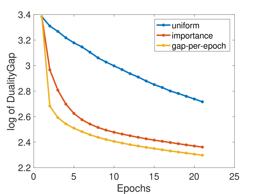
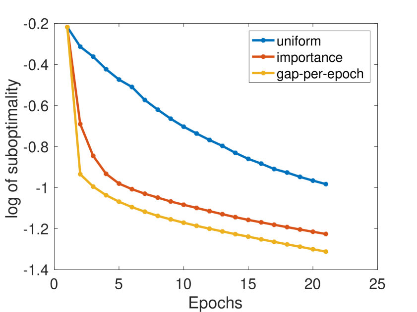
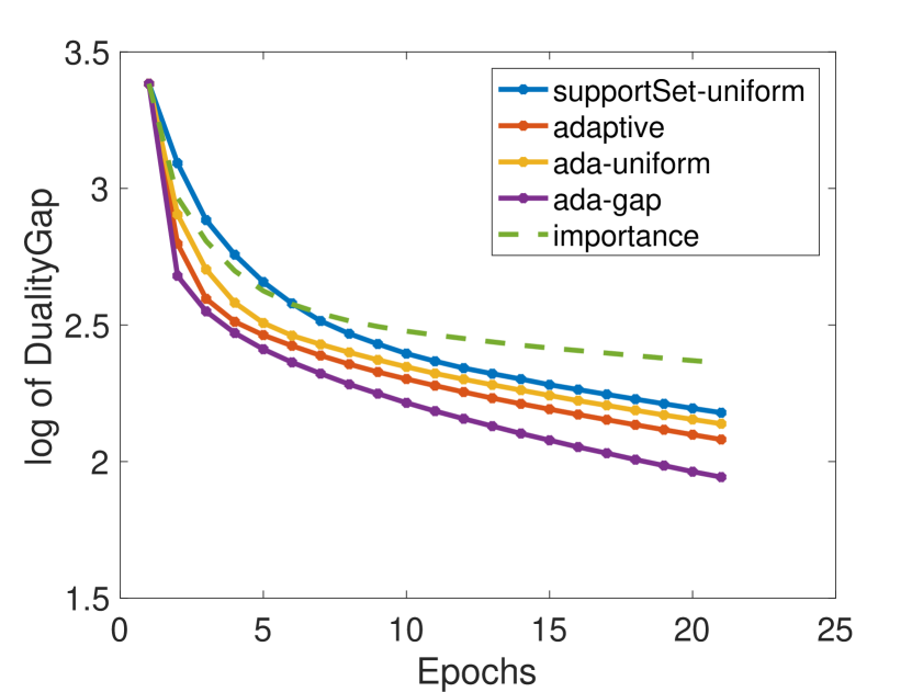
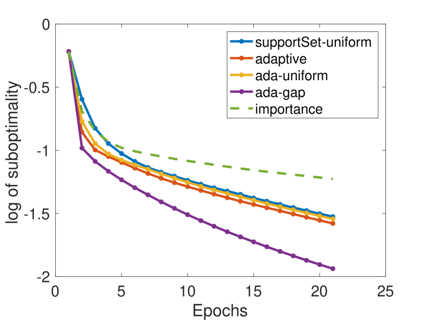
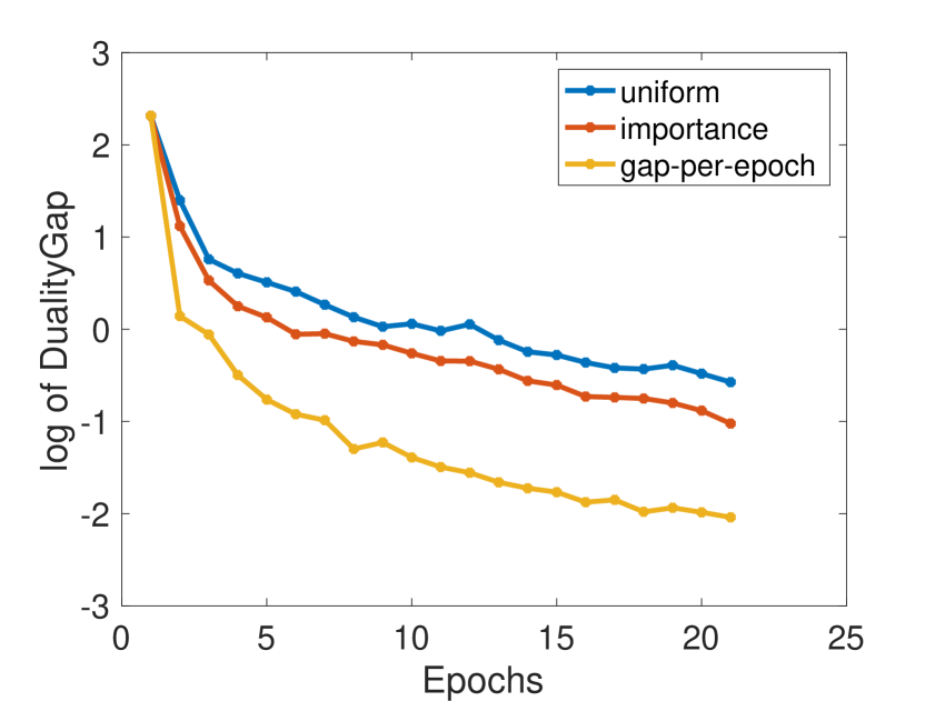
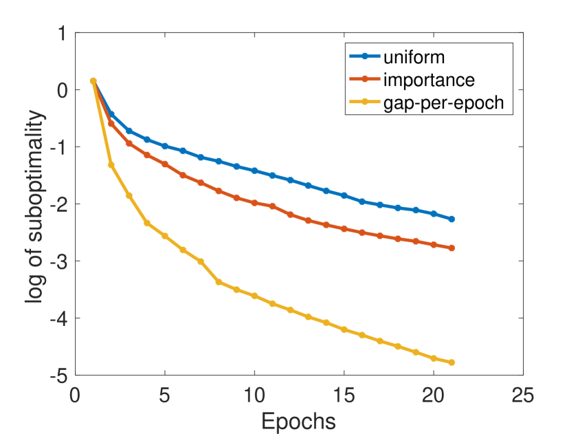
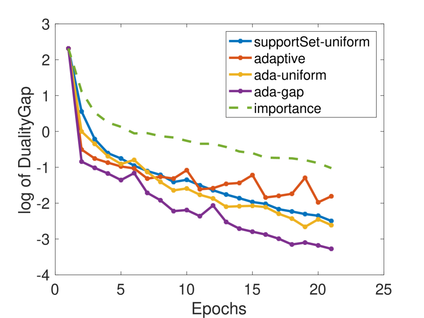
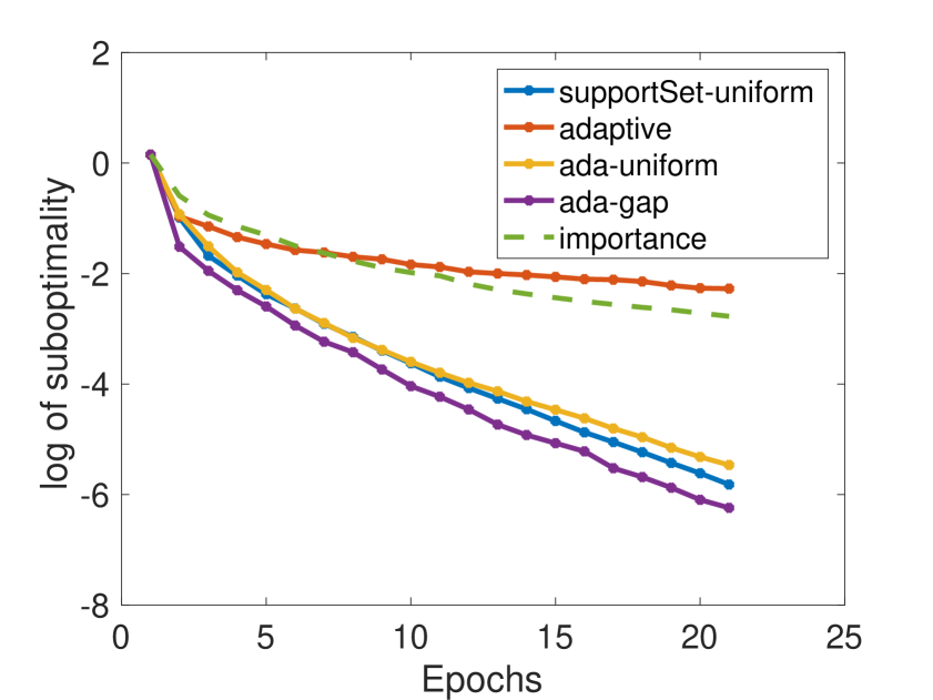
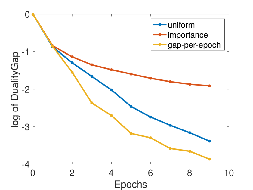
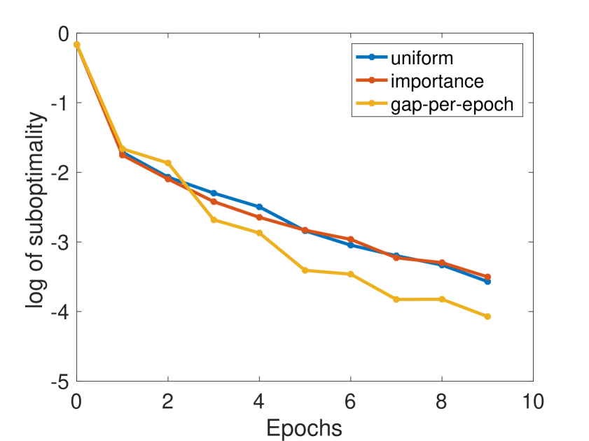
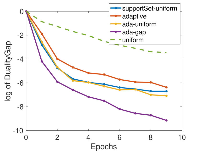
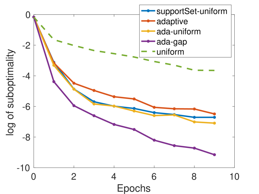
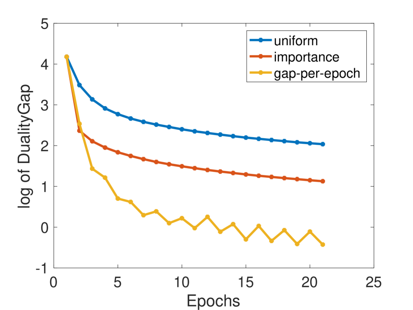
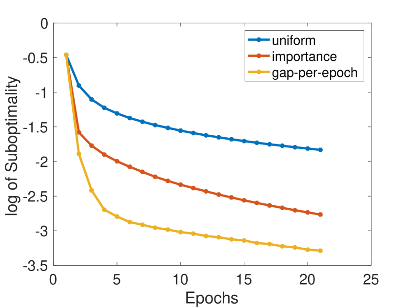
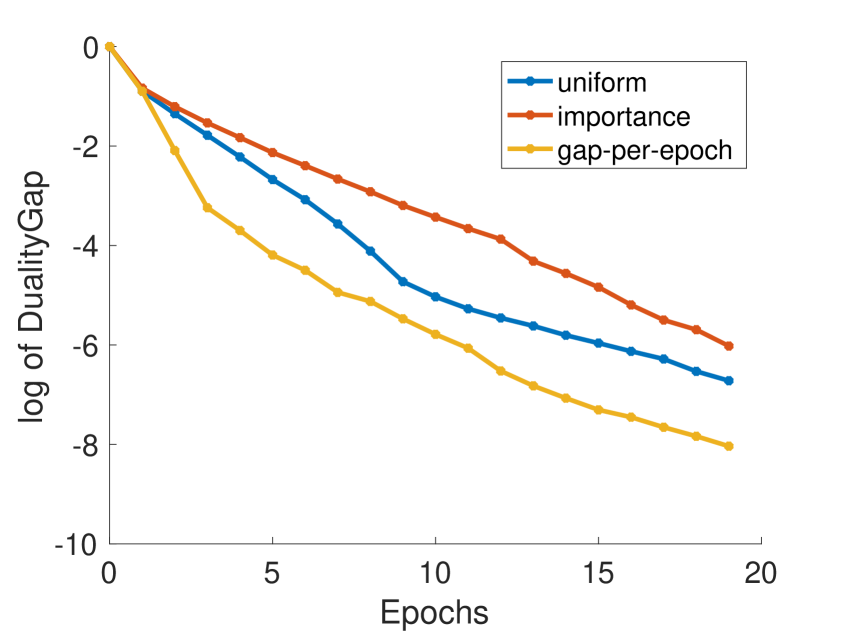
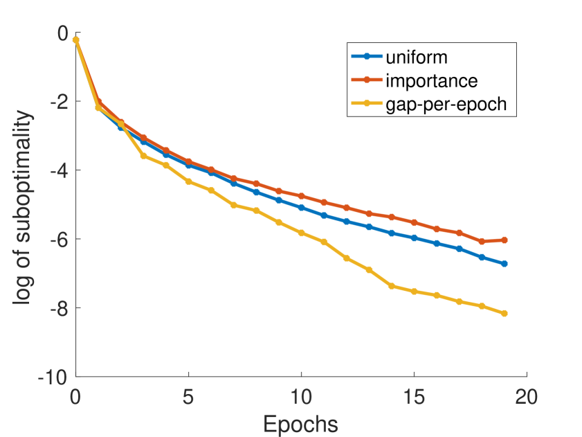
Figure 1: Lasso (first two rows) and SVM (bottom row). Comparison of different fixed and adaptive variants of CD, reporting duality gap and suboptimality measures vs. epochs - rcv1*, mushrooms and ionosphere datasets.
Total cost per epoch

In a naive implementation, the most expensive sampling schemes are adaptive, supportSet-uniform, ada-uniform and ada-gap. Those completely recompute the sampling distribution after each iteration, giving a total per-epoch complexity of 𝒪(nnnz)𝒪𝑛nnz\mathcal{O}(n\cdot\text{nnz}). In contrast, the fixed non-uniform sampling scheme importance requires to build the sampling distribution only once, or once per epoch for gap-per-epoch (both giving 𝒪(nnz)𝒪nnz\mathcal{O}(\text{nnz}) operations). The complexity of n𝑛n samplings using the tree structure is 𝒪(nlog(n))𝒪𝑛𝑛\mathcal{O}(n\log(n)), the complexity of a variable update is 𝒪(nnz)𝒪nnz\mathcal{O}(\text{nnz}). Overall, the asymptotic complexity therefore is 𝒪(nlog(n)+nnz)𝒪𝑛𝑛nnz\mathcal{O}(n\log(n)+\text{nnz}) per epoch, compared to 𝒪(nnz)𝒪nnz\mathcal{O}(\text{nnz}) for simple uniform sampling.

Refer to caption
(a) Gap
Refer to caption
(b) Suboptimality
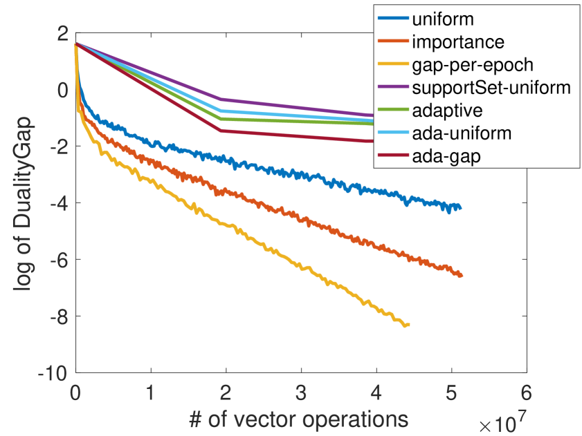
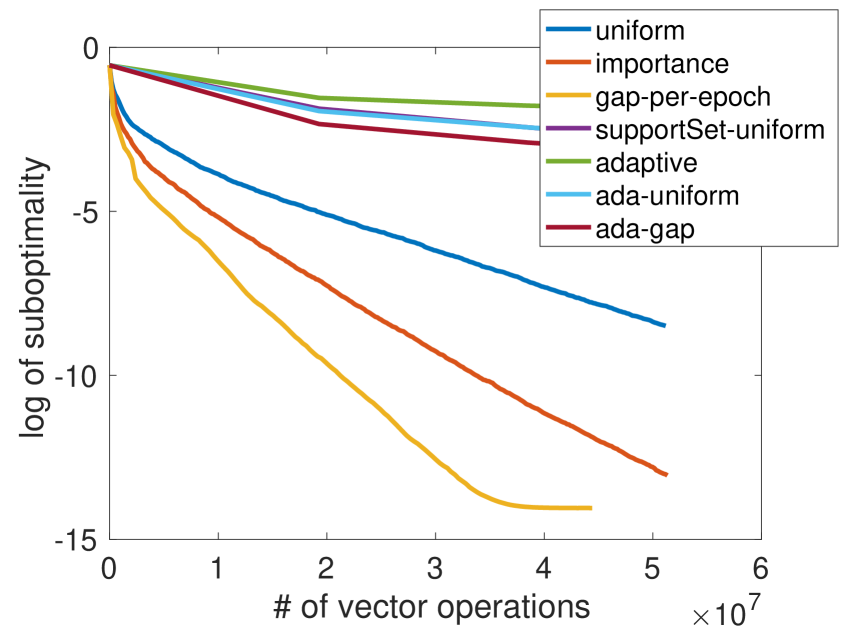
Figure 2: Lasso on the mushrooms dataset. Performance in terms of duality gap and suboptimality, plotted against the total number of vector operations.

5 Experimental results

We provide numerical evidence for our CD sampling strategies on two key machine learning problems: The Lasso and the hinge-loss SVM. All our algorithms and theory are also directly applicable to sparse logistic regression and others, but we omit experiments due to space limitations.

Datasets.

The experiments are performed on three standard datasets listed in Table 2, available111www.csie.ntu.edu.tw/ cjlin/libsvmtools/datasets/ from the UCI repository Asuncion and Newman (2007). Note that rcv1* is a randomly subsampled222We randomly picked 10000 datapoints and 1000 features, and then removed zero rows and columns. version the rcv1 dataset. Experiments on the full rcv1 dataset are provided in Appendix C.

Table 2: Datasets
Dataset d𝑑d n𝑛n nnz/(nd)absent𝑛𝑑/(nd) cv=μ(𝒂i)σ(𝒂i)subscript𝑐𝑣𝜇normsubscript𝒂𝑖𝜎normsubscript𝒂𝑖c_{v}=\frac{\mu(\|\boldsymbol{a}_{i}\|)}{\sigma(\|\boldsymbol{a}_{i}\|)}
mushrooms 112 8124 18.8% 1.34
rcv1* 809 7438 0.3% 0.62
ionosphere 351 33 88% 3.07
Setup.

For Lasso, the regularization parameter λ𝜆\lambda in (20) is set such that the cardinality of the true support set is between 10% and 15 % of the total number of features n𝑛n. We use λ=0.05𝜆0.05\lambda=0.05 for mushrooms, and λ=7104𝜆7superscript104\lambda=7\cdot 10^{-4} for rcv1*. For hinge-loss SVM, the regularization parameter λ𝜆\lambda is chosen such that the classification error on the test set was comparable to training error. We use λ=0.1𝜆0.1\lambda=0.1 for ionosphere.

Performance.

Figures 1 and 2 show the performance of all our studied variants of CD. We record suboptimality and duality gap (see (3)) as the main measures of algorithm performance. All reported results are averaged over 5 runs of each algorithm.

Methods with fixed sampling distributions.

For the three efficient sampling schemes, our results show that CD importance converges faster than CD uniform on both datasets for Lasso, however it is worse than the uniform on SVM. The “mildly” adaptive strategy gap-per-epoch, based on our coordinate-wise duality gap theory but computed only per-epoch, significantly outperforms both of them. This is observed both in number of epochs (Figure 1) as well as number of total vector operations (Figure 2).

Methods with adaptive sampling distributions

For the adaptive methods updating the probabilities after each coordinate step in Figure 1, we show importance sampling as a baseline method (dashed line). We see that measured per epoch, all adaptive methods outperform the fixed sampling methods.Among all adaptive methods, the ada-gap algorithm shows better convergence speed with both suboptimality and duality gap measures.

Highlights.
  • The experiments for Lasso show a clear advantage of non-uniform sampling over the uniform, and superiority of the adaptive sampling over the fixed non-uniform, which is supported by our theory.

  • Among the adaptive methods per iteration, the best performance for both Lasso and SVM in terms of epochs is by ada-gap, which has proven convergence bounds (Theorem 3.7), but also has high computational cost (Θ(dnnz)Θ𝑑nnz\Theta(d\cdot\text{nnz})).

  • The best sampling scheme in terms of total computational cost is gap-per-epoch, which is the epoch-wise variant of the ada-gap algorithm (based on recomputing duality gaps once per epoch), as shown in Figure 2.

6 A discussion on the results

Coordinate descent methods have a rich history in the discipline of optimization as well as many machine learning applications, cf., Wright (2015) for a review.

For SVMs, CD related methods have been studied since their introduction, e.g., by Friess et al. (1998). Hsieh et al. (2008) is the first to propose CD in the partially separable primal-dual setting for hinge-loss. Theoretical convergence rates beyond the application of the hinge-loss can be found in the SDCA line of work Shalev-Shwartz and Zhang (2013), which is the primal-dual analog of the primal-only SGD algorithms. However, the main limitation of SDCA is that it is only applicable to strongly convex regularizers, or requires smoothing techniques Nesterov (2005) to be applicable to general regularizers such as L1. The technique of Dünner et al. (2016) can extend to the CD algorithms as well as the primal-dual analysis to the problem class of interest here, using a bounded set of interest for the iterates instead of relying on smoothing.

The convergence rate of stochastic methods (such as CD and SGD) naturally depends on a sampling probability distribution over the coordinates or datapoints respectively. While virtually all existing methods use sampling uniformly at random Hsieh et al. (2008); Shalev-Shwartz and Tewari (2011); Lacoste-Julien et al. (2013); Shalev-Shwartz and Zhang (2012), recently Nesterov (2012); Qu and Richtárik (2016); Zhao and Zhang (2014); Allen-Zhu et al. (2016) showed that an appropriately defined fixed non-uniform sampling distribution, dubbed as importance sampling, can significantly improve the convergence.

The work of Csiba et al. (2015) has taken the non-uniform sampling a step further towards adaptive sampling. While restricted to strongly convex regularizers, the rates provided for the AdaSDCA algorithm of Csiba et al. (2015) - when updating all probabilities after each step - can beat the ones for uniform and importance sampling. A different approach for adapting the sampling distribution is proposed in Osokin et al. (2016), where the block coordinate Frank-Wolfe algorithm is enhanced with sampling proportional to values of block-wise duality gaps. An adaptive variant of SGD is studied by Papa et al. (2015), where they proposed an adaptive sampling scheme dependent on the past iterations in a Markovian manner, without giving explicit convergence rates. Other adaptive heuristics without proven convergence guarantees include ACF Glasmachers and Dogan (2014) and ACiD Loshchilov et al. (2011).

For general convex regularizers such as L1, the development of CD algorithms includes Fu (1998); Friedman et al. (2007, 2010) and more recent extensions also improving the theoretical convergence rates Shalev-Shwartz and Tewari (2011); Johnson and Guestrin (2015); Zhao et al. (2014). All are restricted to uniform sampling, and we are not aware of proven convergence rates showing improvements of non-uniform or even adaptive sampling for unmodified L1 problems. Zhao and Zhang (2014); Allen-Zhu et al. (2016) show improved rates for non-uniform sampling for L1 but require a smoothing modification of the original problem, and are not covering adaptive sampling.

Conclusion.

In this work, we have investigated adaptive rules for adjusting the sampling probabilities in coordinate descent. Our theoretical results provide improved convergence rates for a more general class of algorithm schemes on one hand, and optimization problems on the other hand, where we are able to directly analyze CD on general convex objectives (as opposed to strongly convex regularizers in previous works). This is particularly useful for L1 problems and (original) hinge-loss objectives, which were not covered by previous schemes. Our practical experiments confirm the strong performance of the adaptive algorithms, and confirm that the behavior predicted by our theory. Finally, we advocate the use of the computationally efficient gap-per-epoch sampling scheme in practice. While the scheme is close to the ones supported by our theory, an explicit primal-dual convergence analysis remains a future research question.

Acknowledgements.

We thank Dominik Csiba and Peter Richtárik for helpful discussions. VC was supported in part by the European Commission under Grant ERC Future Proof, SNF 200021-146750, and SNF CRSII2-147633.

References

  • Allen-Zhu et al. [2016] Zeyuan Allen-Zhu, Zheng Qu, Peter Richtárik, and Yang Yuan. Even Faster Accelerated Coordinate Descent Using Non-Uniform Sampling. In ICML 2016 - Proceedings of the 33th International Conference on Machine Learning, 2016.
  • Asuncion and Newman [2007] A Asuncion and DJ Newman. UCI Machine Learning Repository. Miscellaneous, 2007.
  • Bauschke and Combettes [2011] Heinz H Bauschke and Patrick L Combettes. Convex Analysis and Monotone Operator Theory in Hilbert Spaces. CMS Books in Mathematics. 2011.
  • Csiba et al. [2015] Dominik Csiba, Zheng Qu, and Peter Richtárik. Stochastic Dual Coordinate Ascent with Adaptive Probabilities. In ICML 2015 - Proceedings of the 32th International Conference on Machine Learning, 2015.
  • Dünner et al. [2016] Celestine Dünner, Simone Forte, Martin Takáč, and Martin Jaggi. Primal-Dual Rates and Certificates. In ICML 2016 - Proceedings of the 33th International Conference on Machine Learning, 2016.
  • Friedman et al. [2007] Jerome Friedman, Trevor Hastie, Holger Höfling, and Robert Tibshirani. Pathwise coordinate optimization. The Annals of Applied Statistics, 1(2):302–332, December 2007.
  • Friedman et al. [2010] Jerome Friedman, Trevor Hastie, and Robert Tibshirani. Regularization Paths for Generalized Linear Models via Coordinate Descent. Journal of Statistical Software, 33(1):1–22, 2010.
  • Friess et al. [1998] Thilo-Thomas Friess, Nello Cristianini, and Colin Campbell. The kernel-adatron algorithm: a fast and simple learning procedure for support vector machines. ICML 1998 - Proceedings of the 15th International Conference on Machine Learning, 1998.
  • Fu [1998] Wenjiang J. Fu. Penalized regressions: The bridge versus the lasso. Journal of Computational and Graphical Statistics, 7(3):397–416, 1998.
  • Glasmachers and Dogan [2014] Tobias Glasmachers and Ürün Dogan. Coordinate Descent with Online Adaptation of Coordinate Frequencies. arXiv, 2014.
  • Hsieh et al. [2008] Cho-Jui Hsieh, Kai-Wei Chang, Chih-Jen Lin, S Sathiya Keerthi, and S Sundararajan. A Dual Coordinate Descent Method for Large-scale Linear SVM. ICML - the 25th International Conference on Machine Learning, 2008.
  • Johnson and Guestrin [2015] Tyler Johnson and Carlos Guestrin. Blitz: A Principled Meta-Algorithm for Scaling Sparse Optimization. In ICML 2015 - Proceedings of the 32th International Conference on Machine Learning, 2015.
  • Lacoste-Julien et al. [2013] Simon Lacoste-Julien, Martin Jaggi, Mark Schmidt, and Patrick Pletscher. Block-Coordinate Frank-Wolfe Optimization for Structural SVMs. In ICML 2013 - Proceedings of the 30th International Conference on Machine Learning, 2013.
  • Loshchilov et al. [2011] Ilya Loshchilov, Marc Schoenauer, and Michèle Sebag. Adaptive Coordinate Descent. In Natalio Krasnogor and Pier Luca Lanzi, editors, Genetic and Evolutionary Computation Conference (GECCO 2011), pages 885–992, Dublin, Ireland, 2011. ACM-SIGEVO.
  • Necorara et al. [2012] I Necorara, Yurii Nesterov, and François Glineur. Efficiency of Randomized Coordinate Descent Methods on Optimization Problems With Linearly Coupled Constraints. Technical Report, 2012.
  • Nesterov [2005] Yurii Nesterov. Smooth minimization of non-smooth functions. Mathematical Programming, 103(1):127–152, 2005.
  • Nesterov [2012] Yurii Nesterov. Efficiency of Coordinate Descent Methods on Huge-Scale Optimization Problems. SIAM Journal on Optimization, 22(2):341–362, 2012.
  • Nesterov [2013] Yurii Nesterov. Subgradient methods for huge-scale optimization problems. Mathematical Programming, 146(1-2):275–297, 2013.
  • Osokin et al. [2016] Anton Osokin, Jean-Baptiste Alayrac, Isabella Lukasewitz, Puneet Dokania, and Simon Lacoste-Julien. Minding the Gaps for Block Frank-Wolfe Optimization of Structured SVMs. In ICML 2016 - Proceedings of the 33th International Conference on Machine Learning, 2016.
  • Papa et al. [2015] Guillaume Papa, Pascal Bianchi, and Stéphan Clémençon. Adaptive Sampling for Incremental Optimization Using Stochastic Gradient Descent. In ALT - 26th International Conference on Algorithmic Learning Theory, pages 317–331. 2015.
  • Qu and Richtárik [2016] Zheng Qu and Peter Richtárik. Coordinate descent with arbitrary sampling I: algorithms and complexity. Optimization Methods and Software, 31(5):829–857, 2016.
  • Shalev-Shwartz and Tewari [2011] Shai Shalev-Shwartz and Ambuj Tewari. Stochastic Methods for l1-regularized Loss Minimization. JMLR, 12:1865–1892, 2011.
  • Shalev-Shwartz and Wexler [2016] Shai Shalev-Shwartz and Yonatan Wexler. Minimizing the Maximal Loss: How and Why? arXiv, 2016.
  • Shalev-Shwartz and Zhang [2012] Shai Shalev-Shwartz and Tong Zhang. Proximal Stochastic Dual Coordinate Ascent. arXiv, 2012.
  • Shalev-Shwartz and Zhang [2013] Shai Shalev-Shwartz and Tong Zhang. Stochastic Dual Coordinate Ascent Methods for Regularized Loss Minimization. JMLR, 14:567–599, 2013.
  • Wright [2015] Stephen J Wright. Coordinate descent algorithms. Mathematical Programming, 151(1):3–34, 2015.
  • Zhao and Zhang [2014] Peilin Zhao and Tong Zhang. Stochastic Optimization with Importance Sampling. arXiv, 2014.
  • Zhao et al. [2014] Tuo Zhao, Han Liu, and Tong Zhang. Pathwise Coordinate Optimization for Sparse Learning: Algorithm and Theory. arXiv, 2014.

Appendix A Proofs

Lemma’ 3.1.

Let f𝑓f be 1/β1𝛽1/\beta-smooth and each gisubscript𝑔𝑖g_{i} be μisubscript𝜇𝑖\mu_{i}-strongly convex with convexity parameter μi0subscript𝜇𝑖0\mu_{i}\geq 0 i[n]for-all𝑖delimited-[]𝑛\forall i\in[n]. For the case μi=0subscript𝜇𝑖0\mu_{i}=0, we require gisubscript𝑔𝑖g_{i} to have a bounded support. Then for any iteration t𝑡t, any sampling distribution 𝐩(t)superscript𝐩𝑡\boldsymbol{p}^{(t)} and any arbitrary si[0,1]subscript𝑠𝑖01s_{i}\in[0,1] i[n]for-all𝑖delimited-[]𝑛\forall i\in[n], the iterates of the CD method satisfy

𝔼[𝒪A(𝜶(t+1))|𝜶(t)]𝒪A(𝜶(t))isipi(t)Gi(𝜶(t))𝔼delimited-[]conditionalsubscript𝒪𝐴superscript𝜶𝑡1superscript𝜶𝑡subscript𝒪𝐴superscript𝜶𝑡subscript𝑖subscript𝑠𝑖superscriptsubscript𝑝𝑖𝑡subscript𝐺𝑖superscript𝜶𝑡\displaystyle\mathbb{E}[\mathcal{O}_{A}(\boldsymbol{\alpha}^{(t+1)})|\boldsymbol{\alpha}^{(t)}]\leq\mathcal{O}_{A}(\boldsymbol{\alpha}^{(t)})-\sum_{i}s_{i}p_{i}^{(t)}G_{i}(\boldsymbol{\alpha}^{(t)}) (23)
ipi(t)(μi(sisi2)2si2𝒂i22β)|κi(t)|2,subscript𝑖superscriptsubscript𝑝𝑖𝑡subscript𝜇𝑖subscript𝑠𝑖superscriptsubscript𝑠𝑖22superscriptsubscript𝑠𝑖2superscriptnormsubscript𝒂𝑖22𝛽superscriptsuperscriptsubscript𝜅𝑖𝑡2\displaystyle-\sum_{i}p_{i}^{(t)}\Big{(}\frac{\mu_{i}(s_{i}-s_{i}^{2})}{2}-\frac{s_{i}^{2}\|\boldsymbol{a}_{i}\|^{2}}{2\beta}\Big{)}|\kappa_{i}^{(t)}|^{2},

here κi(t)superscriptsubscript𝜅𝑖𝑡\kappa_{i}^{(t)} is i𝑖i-th dual residual.

Proof.

Since in CD update (𝜶(t+1)=𝜶(t)+𝒆iΔαisuperscript𝜶𝑡1superscript𝜶𝑡subscript𝒆𝑖Δsubscript𝛼𝑖\boldsymbol{\alpha}^{(t+1)}=\boldsymbol{\alpha}^{(t)}+\boldsymbol{e}_{i}\Delta\alpha_{i}) only one coordinate per iteration is changed, the one iteration improvement in dual objective can be written as:

𝒪A(𝜶(t))𝒪A(𝜶(t+1))subscript𝒪𝐴superscript𝜶𝑡subscript𝒪𝐴superscript𝜶𝑡1\displaystyle\mathcal{O}_{A}(\boldsymbol{\alpha}^{(t)})-\mathcal{O}_{A}(\boldsymbol{\alpha}^{(t+1)})
=[gi(αi(t))+f(A𝜶(t))](A)[gi(αi(t+1))+f(A𝜶(t+1))](B).absentsubscriptdelimited-[]subscript𝑔𝑖superscriptsubscript𝛼𝑖𝑡𝑓𝐴superscript𝜶𝑡𝐴subscriptdelimited-[]subscript𝑔𝑖superscriptsubscript𝛼𝑖𝑡1𝑓𝐴superscript𝜶𝑡1𝐵\displaystyle=\underbrace{\Big{[}g_{i}(\alpha_{i}^{(t)})+f(A\boldsymbol{\alpha}^{(t)})\Big{]}}_{(A)}-\underbrace{\Big{[}g_{i}(\alpha_{i}^{(t+1)})+f(A\boldsymbol{\alpha}^{(t+1)})\Big{]}}_{(B)}.

To bound part (B)𝐵(B) we use a suboptimal update Δαi=siκi(t)Δsubscript𝛼𝑖subscript𝑠𝑖superscriptsubscript𝜅𝑖𝑡\Delta\alpha_{i}=s_{i}\kappa_{i}^{(t)}, for all si[0,1]subscript𝑠𝑖01s_{i}\in[0,1]:

(B)𝐵\displaystyle(B) =gi(αi(t+1))+f(A𝜶(t+1))absentsubscript𝑔𝑖superscriptsubscript𝛼𝑖𝑡1𝑓𝐴superscript𝜶𝑡1\displaystyle=g_{i}(\alpha_{i}^{(t+1)})+f(A\boldsymbol{\alpha}^{(t+1)})
minΔαi[gi(αi(t)+Δαi)+f(A𝜶(t)+𝒂iΔαi)]absentsubscriptΔsubscript𝛼𝑖subscript𝑔𝑖superscriptsubscript𝛼𝑖𝑡Δsubscript𝛼𝑖𝑓𝐴superscript𝜶𝑡subscript𝒂𝑖Δsubscript𝛼𝑖\displaystyle\leq\min_{\Delta\alpha_{i}}\Big{[}g_{i}(\alpha_{i}^{(t)}+\Delta\alpha_{i})+f(A\boldsymbol{\alpha}^{(t)}+\boldsymbol{a}_{i}\Delta\alpha_{i})\Big{]}
gi(αi(t)+siκi(t))+f(A𝜶(t)+𝒂isiκi(t)).absentsubscript𝑔𝑖superscriptsubscript𝛼𝑖𝑡subscript𝑠𝑖superscriptsubscript𝜅𝑖𝑡𝑓𝐴superscript𝜶𝑡subscript𝒂𝑖subscript𝑠𝑖superscriptsubscript𝜅𝑖𝑡\displaystyle\leq g_{i}(\alpha_{i}^{(t)}+s_{i}\kappa_{i}^{(t)})+f(A\boldsymbol{\alpha}^{(t)}+\boldsymbol{a}_{i}s_{i}\kappa_{i}^{(t)}).

Each of gisubscript𝑔𝑖g_{i} is μisubscript𝜇𝑖\mu_{i}-strongly convex, therefore:

gi(αi(t)+siκi(t))=gi(αi(t)+si(ui(t)αi(t)))subscript𝑔𝑖superscriptsubscript𝛼𝑖𝑡subscript𝑠𝑖superscriptsubscript𝜅𝑖𝑡subscript𝑔𝑖superscriptsubscript𝛼𝑖𝑡subscript𝑠𝑖superscriptsubscript𝑢𝑖𝑡superscriptsubscript𝛼𝑖𝑡\displaystyle g_{i}(\alpha_{i}^{(t)}+s_{i}\kappa_{i}^{(t)})=g_{i}(\alpha_{i}^{(t)}+s_{i}(u_{i}^{(t)}-\alpha_{i}^{(t)}))
=gi(si(ui(t))+(1si)(αi(t)))absentsubscript𝑔𝑖subscript𝑠𝑖superscriptsubscript𝑢𝑖𝑡1subscript𝑠𝑖superscriptsubscript𝛼𝑖𝑡\displaystyle=g_{i}(s_{i}(u_{i}^{(t)})+(1-s_{i})(\alpha_{i}^{(t)}))
sigi(ui(t))+(1si)gi(αi(t))μi2si(1si)(κi(t))2.absentsubscript𝑠𝑖subscript𝑔𝑖superscriptsubscript𝑢𝑖𝑡1subscript𝑠𝑖subscript𝑔𝑖superscriptsubscript𝛼𝑖𝑡subscript𝜇𝑖2subscript𝑠𝑖1subscript𝑠𝑖superscriptsuperscriptsubscript𝜅𝑖𝑡2\displaystyle\leq s_{i}g_{i}(u_{i}^{(t)})+(1-s_{i})g_{i}(\alpha_{i}^{(t)})-\frac{\mu_{i}}{2}s_{i}(1-s_{i})(\kappa_{i}^{(t)})^{2}.

The function f𝑓f is 1β1𝛽\frac{1}{\beta}-smooth:

f(A𝜶(t)+𝒂isiκi(t))𝑓𝐴superscript𝜶𝑡subscript𝒂𝑖subscript𝑠𝑖superscriptsubscript𝜅𝑖𝑡\displaystyle f(A\boldsymbol{\alpha}^{(t)}+\boldsymbol{a}_{i}s_{i}\kappa_{i}^{(t)})
f(A𝜶(t))+f(A𝜶(t))(siκi(t)𝒂i)+12βsiκi(t)𝒂i2.absent𝑓𝐴superscript𝜶𝑡𝑓superscript𝐴superscript𝜶𝑡topsubscript𝑠𝑖superscriptsubscript𝜅𝑖𝑡subscript𝒂𝑖12𝛽superscriptnormsubscript𝑠𝑖superscriptsubscript𝜅𝑖𝑡subscript𝒂𝑖2\displaystyle\leq f(A\boldsymbol{\alpha}^{(t)})+\nabla f(A\boldsymbol{\alpha}^{(t)})^{\top}(s_{i}\kappa_{i}^{(t)}\boldsymbol{a}_{i})+\frac{1}{2\beta}\|s_{i}\kappa_{i}^{(t)}\boldsymbol{a}_{i}\|^{2}.

As a result:

(B)𝐵\displaystyle(B) sigi(ui(t))sigi(αi(t))μi2si(1si)(κi(t))2absentsubscript𝑠𝑖subscript𝑔𝑖superscriptsubscript𝑢𝑖𝑡subscript𝑠𝑖subscript𝑔𝑖superscriptsubscript𝛼𝑖𝑡subscript𝜇𝑖2subscript𝑠𝑖1subscript𝑠𝑖superscriptsuperscriptsubscript𝜅𝑖𝑡2\displaystyle\leq s_{i}g_{i}(u_{i}^{(t)})-s_{i}g_{i}(\alpha_{i}^{(t)})-\frac{\mu_{i}}{2}s_{i}(1-s_{i})(\kappa_{i}^{(t)})^{2}
+gi(αi(t))+f(A𝜶(t))(A)+f(A𝜶(t))(siκi(t)𝒂i)subscriptsubscript𝑔𝑖superscriptsubscript𝛼𝑖𝑡𝑓𝐴superscript𝜶𝑡𝐴𝑓superscript𝐴superscript𝜶𝑡topsubscript𝑠𝑖superscriptsubscript𝜅𝑖𝑡subscript𝒂𝑖\displaystyle+\underbrace{g_{i}(\alpha_{i}^{(t)})+f(A\boldsymbol{\alpha}^{(t)})}_{(A)}+\nabla f(A\boldsymbol{\alpha}^{(t)})^{\top}(s_{i}\kappa_{i}^{(t)}\boldsymbol{a}_{i})
+12βsiκi(t)𝒂i2.12𝛽superscriptnormsubscript𝑠𝑖superscriptsubscript𝜅𝑖𝑡subscript𝒂𝑖2\displaystyle+\frac{1}{2\beta}\|s_{i}\kappa_{i}^{(t)}\boldsymbol{a}_{i}\|^{2}.

With obtained results above and optimality condition 𝒘(𝜶)=f(A𝜶)𝒘𝜶𝑓𝐴𝜶\boldsymbol{w}(\boldsymbol{\alpha})=\nabla f(A\boldsymbol{\alpha}), the improvement in dual objective can be written as:

𝒪A(𝜶(t))𝒪A(𝜶(t+1))=(A)(B)subscript𝒪𝐴superscript𝜶𝑡subscript𝒪𝐴superscript𝜶𝑡1𝐴𝐵\displaystyle\mathcal{O}_{A}(\boldsymbol{\alpha}^{(t)})-\mathcal{O}_{A}(\boldsymbol{\alpha}^{(t+1)})=(A)-(B)
sigi(ui(t))+sigi(αi(t))+μi2si(1si)(κi(t))2absentsubscript𝑠𝑖subscript𝑔𝑖superscriptsubscript𝑢𝑖𝑡subscript𝑠𝑖subscript𝑔𝑖superscriptsubscript𝛼𝑖𝑡subscript𝜇𝑖2subscript𝑠𝑖1subscript𝑠𝑖superscriptsuperscriptsubscript𝜅𝑖𝑡2\displaystyle\geq-s_{i}g_{i}(u_{i}^{(t)})+s_{i}g_{i}(\alpha_{i}^{(t)})+\frac{\mu_{i}}{2}s_{i}(1-s_{i})(\kappa_{i}^{(t)})^{2}
𝒘(𝜶(t))(siui(t)𝒂i)+𝒘(𝜶(t))(siαi(t)𝒂i)12βsiκi(t)𝒂i2𝒘superscript𝜶𝑡subscript𝑠𝑖superscriptsubscript𝑢𝑖𝑡subscript𝒂𝑖𝒘superscript𝜶𝑡subscript𝑠𝑖superscriptsubscript𝛼𝑖𝑡subscript𝒂𝑖12𝛽superscriptnormsubscript𝑠𝑖superscriptsubscript𝜅𝑖𝑡subscript𝒂𝑖2\displaystyle-\boldsymbol{w}(\boldsymbol{\alpha}^{(t)})(s_{i}u_{i}^{(t)}\boldsymbol{a}_{i})+\boldsymbol{w}(\boldsymbol{\alpha}^{(t)})(s_{i}\alpha_{i}^{(t)}\boldsymbol{a}_{i})-\frac{1}{2\beta}\|s_{i}\kappa_{i}^{(t)}\boldsymbol{a}_{i}\|^{2}
=si(gi(ui(t))+gi(αi(t))𝒘(𝜶(t))(uit1𝒂i)\displaystyle=s_{i}\Big{(}-g_{i}(u_{i}^{(t)})+g_{i}(\alpha_{i}^{(t)})-\boldsymbol{w}(\boldsymbol{\alpha}^{(t)})(u_{i}^{t-1}\boldsymbol{a}_{i})
+𝒘(𝜶(t))(αit1𝒂i)+μi2(1si)(κi(t))2si2β𝒂i2|κi(t)|2).\displaystyle+\boldsymbol{w}(\boldsymbol{\alpha}^{(t)})(\alpha_{i}^{t-1}\boldsymbol{a}_{i})+\frac{\mu_{i}}{2}(1-s_{i})(\kappa_{i}^{(t)})^{2}-\frac{s_{i}}{2\beta}\|\boldsymbol{a}_{i}\|^{2}|\kappa_{i}^{(t)}|^{2}\Big{)}.

Since ui(t)gi(𝒂i𝒘(𝜶(t)))superscriptsubscript𝑢𝑖𝑡superscriptsubscript𝑔𝑖superscriptsubscript𝒂𝑖top𝒘superscript𝜶𝑡u_{i}^{(t)}\in\partial g_{i}^{*}(-\boldsymbol{a}_{i}^{\top}\boldsymbol{w}(\boldsymbol{\alpha}^{(t)})), the Fenchel-Young inequality becomes equality for gi(ui(t))subscript𝑔𝑖superscriptsubscript𝑢𝑖𝑡g_{i}(u_{i}^{(t)}):

gi(ui(t))+gi(𝒂i𝒘(𝜶(t)))=𝒘(𝜶(t))(ui(t)𝒂i)subscript𝑔𝑖superscriptsubscript𝑢𝑖𝑡superscriptsubscript𝑔𝑖superscriptsubscript𝒂𝑖top𝒘superscript𝜶𝑡𝒘superscript𝜶𝑡superscriptsubscript𝑢𝑖𝑡subscript𝒂𝑖g_{i}(u_{i}^{(t)})+g_{i}^{*}(-\boldsymbol{a}_{i}^{\top}\boldsymbol{w}(\boldsymbol{\alpha}^{(t)}))=-\boldsymbol{w}(\boldsymbol{\alpha}^{(t)})(u_{i}^{(t)}\boldsymbol{a}_{i})

Using this fact, the bound on the improvement in dual objective becomes:

𝒪A(𝜶(t))𝒪A(𝜶(t+1))si(gi(αi(t))+gi(𝒂i𝒘(𝜶(t)))\displaystyle\mathcal{O}_{A}(\boldsymbol{\alpha}^{(t)})-\mathcal{O}_{A}(\boldsymbol{\alpha}^{(t+1)})\geq s_{i}\Big{(}g_{i}(\alpha_{i}^{(t)})+g_{i}^{*}(-\boldsymbol{a}_{i}^{\top}\boldsymbol{w}(\boldsymbol{\alpha}^{(t)}))
+𝒘(𝜶(t))(αi(t)𝒂i)+μi2(1si)(κi(t))2si2β𝒂i2|κi(t)|2)\displaystyle+\boldsymbol{w}(\boldsymbol{\alpha}^{(t)})(\alpha_{i}^{(t)}\boldsymbol{a}_{i})+\frac{\mu_{i}}{2}(1-s_{i})(\kappa_{i}^{(t)})^{2}-\frac{s_{i}}{2\beta}\|\boldsymbol{a}_{i}\|^{2}|\kappa_{i}^{(t)}|^{2}\Big{)}

Therefore for any si[0,1]subscript𝑠𝑖01s_{i}\in[0,1] it holds that:

𝒪A(𝜶(t))𝒪A(𝜶(t+1))subscript𝒪𝐴superscript𝜶𝑡subscript𝒪𝐴superscript𝜶𝑡1\displaystyle\mathcal{O}_{A}(\boldsymbol{\alpha}^{(t)})-\mathcal{O}_{A}(\boldsymbol{\alpha}^{(t+1)}) (24)
si[Gi(𝜶(t))+μi2(1si)|κi(t)|2si2β𝒂i2|κi(t)|2],absentsubscript𝑠𝑖delimited-[]subscript𝐺𝑖superscript𝜶𝑡subscript𝜇𝑖21subscript𝑠𝑖superscriptsuperscriptsubscript𝜅𝑖𝑡2subscript𝑠𝑖2𝛽superscriptnormsubscript𝒂𝑖2superscriptsuperscriptsubscript𝜅𝑖𝑡2\displaystyle\geq s_{i}\Big{[}G_{i}(\boldsymbol{\alpha}^{(t)})+\frac{\mu_{i}}{2}(1-s_{i})|\kappa_{i}^{(t)}|^{2}-\frac{s_{i}}{2\beta}\|\boldsymbol{a}_{i}\|^{2}|\kappa_{i}^{(t)}|^{2}\Big{]},

where Gisubscript𝐺𝑖G_{i} is i𝑖i-th coordinate-wise duality gap:

G(𝜶(t))=iGi(𝜶(t))𝐺superscript𝜶𝑡subscript𝑖subscript𝐺𝑖superscript𝜶𝑡\displaystyle G(\boldsymbol{\alpha}^{(t)})=\sum_{i}G_{i}(\boldsymbol{\alpha}^{(t)})
Gi(𝜶(t))=gi(𝒂i𝒘)+gi(αi(t))+αi(t)𝒂i𝒘.subscript𝐺𝑖superscript𝜶𝑡superscriptsubscript𝑔𝑖superscriptsubscript𝒂𝑖top𝒘subscript𝑔𝑖superscriptsubscript𝛼𝑖𝑡superscriptsubscript𝛼𝑖𝑡superscriptsubscript𝒂𝑖top𝒘\displaystyle G_{i}(\boldsymbol{\alpha}^{(t)})=g_{i}^{*}(-\boldsymbol{a}_{i}^{\top}\boldsymbol{w})+g_{i}(\alpha_{i}^{(t)})+\alpha_{i}^{(t)}\boldsymbol{a}_{i}^{\top}\boldsymbol{w}.

By taking an expectation of the both sides with respect to i𝑖i, conditioned on 𝜶(t)superscript𝜶𝑡\boldsymbol{\alpha}^{(t)}, we obtain:

𝔼[𝒪A(𝜶(t+1))|𝜶(t)]𝒪A(𝜶(t))isipi(t)Gi(𝜶(t))𝔼delimited-[]conditionalsubscript𝒪𝐴superscript𝜶𝑡1superscript𝜶𝑡subscript𝒪𝐴superscript𝜶𝑡subscript𝑖subscript𝑠𝑖superscriptsubscript𝑝𝑖𝑡subscript𝐺𝑖superscript𝜶𝑡\displaystyle\mathbb{E}[\mathcal{O}_{A}(\boldsymbol{\alpha}^{(t+1)})|\boldsymbol{\alpha}^{(t)}]\leq\mathcal{O}_{A}(\boldsymbol{\alpha}^{(t)})-\sum_{i}s_{i}p_{i}^{(t)}G_{i}(\boldsymbol{\alpha}^{(t)})
ipi(t)(μi(sisi2)2si2𝒂i22β)|κi(t)|2subscript𝑖superscriptsubscript𝑝𝑖𝑡subscript𝜇𝑖subscript𝑠𝑖superscriptsubscript𝑠𝑖22superscriptsubscript𝑠𝑖2superscriptnormsubscript𝒂𝑖22𝛽superscriptsuperscriptsubscript𝜅𝑖𝑡2\displaystyle-\sum_{i}p_{i}^{(t)}\Big{(}\frac{\mu_{i}(s_{i}-s_{i}^{2})}{2}-\frac{s_{i}^{2}\|\boldsymbol{a}_{i}\|^{2}}{2\beta}\Big{)}|\kappa_{i}^{(t)}|^{2}

and thus finalize the proof. ∎

Theorem’ 3.3.

Assume f𝑓f is 1β1𝛽\frac{1}{\beta}-smooth function. Then, if gisubscriptsuperscript𝑔𝑖g^{*}_{i} is Lisubscript𝐿𝑖L_{i}-Lipschitz for each i𝑖i and 𝐩(t)superscript𝐩𝑡\boldsymbol{p}^{(t)} is coherent with 𝛋(t)superscript𝛋𝑡\boldsymbol{\kappa}^{(t)}, then the iterates of the CD method satisfies

𝔼[εA(t)]2Fn2+2εA(0)pmin2pmin+t.𝔼delimited-[]superscriptsubscript𝜀𝐴𝑡2superscript𝐹superscript𝑛22superscriptsubscript𝜀𝐴0subscript𝑝2subscript𝑝𝑡\mathbb{E}[\varepsilon_{A}^{(t)}]\leq\frac{2F^{\circ}n^{2}+\frac{2\varepsilon_{A}^{(0)}}{p_{\min}}}{\frac{2}{p_{\min}}+t}. (25)

Moreover, the overall number of iterations T𝑇T to obtain a duality gap G(𝛂¯)ε𝐺¯𝛂𝜀G(\bar{\boldsymbol{\alpha}})\leq\varepsilon must satisfy the following:

Tmax{0,1pminlog(2εA(0)n2pminF)}+5Fn2ε1pmin.𝑇01subscript𝑝2superscriptsubscript𝜀𝐴0superscript𝑛2subscript𝑝superscript𝐹5superscript𝐹superscript𝑛2𝜀1subscript𝑝T\geq\max\Bigg{\{}0,\frac{1}{p_{\min}}\log\Big{(}\frac{2\varepsilon_{A}^{(0)}}{n^{2}p_{\min}F^{\circ}}\Big{)}\Bigg{\}}+\frac{5F^{\circ}n^{2}}{\varepsilon}-\frac{1}{p_{\min}}. (26)

Moreover, when tT0𝑡subscript𝑇0t\geq T_{0} with

T0=max{0,1pminlog(2εA(0)n2pminF)}+4Fn2ε2pminsubscript𝑇001subscript𝑝2superscriptsubscript𝜀𝐴0superscript𝑛2subscript𝑝superscript𝐹4superscript𝐹superscript𝑛2𝜀2subscript𝑝T_{0}=\max\Bigg{\{}0,\frac{1}{p_{\min}}\log\Big{(}\frac{2\varepsilon_{A}^{(0)}}{n^{2}p_{\min}F^{\circ}}\Big{)}\Bigg{\}}+\frac{4F^{\circ}n^{2}}{\varepsilon}-\frac{2}{p_{\min}} (27)

we have the suboptimality bound of 𝔼[𝒪A(𝛂(t))𝒪A(𝛂)]ε/2𝔼delimited-[]subscript𝒪𝐴superscript𝛂𝑡subscript𝒪𝐴superscript𝛂𝜀2\mathbb{E}[\mathcal{O}_{A}(\boldsymbol{\alpha}^{(t)})-\mathcal{O}_{A}(\boldsymbol{\alpha}^{\star})]\leq\varepsilon/2, where εA(0)subscriptsuperscript𝜀0𝐴\varepsilon^{(0)}_{A} is the initial dual suboptimality and Fsuperscript𝐹F^{\circ} is an upper bound on 𝔼[F(t)]𝔼delimited-[]superscript𝐹𝑡\mathbb{E}[F^{(t)}] taken over the random choice of the sampled coordinate at 1,,T01subscript𝑇01,\dots,T_{0} algorithm iterations.

Proof.

According to Lemma 2.2 if gisubscriptsuperscript𝑔𝑖g^{*}_{i} is Lisubscript𝐿𝑖L_{i}-Lipschitz, then gisubscript𝑔𝑖g_{i} has Lisubscript𝐿𝑖L_{i}-bounded support and the conditions of Remark 3.2 are satisfied. From Remark 3.2 we know:

𝔼[𝒪A(𝜶(t+1))|𝜶(t)]𝒪A(𝜶(t))θG(𝜶(t))+θ2n22F(t)𝔼delimited-[]conditionalsubscript𝒪𝐴superscript𝜶𝑡1superscript𝜶𝑡subscript𝒪𝐴superscript𝜶𝑡𝜃𝐺superscript𝜶𝑡superscript𝜃2superscript𝑛22superscript𝐹𝑡\mathbb{E}[\mathcal{O}_{A}(\boldsymbol{\alpha}^{(t+1)})|\boldsymbol{\alpha}^{(t)}]\leq\mathcal{O}_{A}(\boldsymbol{\alpha}^{(t)})-\theta G(\boldsymbol{\alpha}^{(t)})+\frac{\theta^{2}n^{2}}{2}F^{(t)} (28)

With 𝒪A(𝜶(t))𝒪A(𝜶(t+1))=εA(t)εA(t+1)subscript𝒪𝐴superscript𝜶𝑡subscript𝒪𝐴superscript𝜶𝑡1superscriptsubscript𝜀𝐴𝑡superscriptsubscript𝜀𝐴𝑡1\mathcal{O}_{A}(\boldsymbol{\alpha}^{(t)})-\mathcal{O}_{A}(\boldsymbol{\alpha}^{(t+1)})=\varepsilon_{A}^{(t)}-\varepsilon_{A}^{(t+1)} and εA(t)=𝒪A(𝜶(t))𝒪A(𝜶)G(𝜶(t)),superscriptsubscript𝜀𝐴𝑡subscript𝒪𝐴superscript𝜶𝑡subscript𝒪𝐴superscript𝜶𝐺superscript𝜶𝑡\varepsilon_{A}^{(t)}=\mathcal{O}_{A}(\boldsymbol{\alpha}^{(t)})-\mathcal{O}_{A}(\boldsymbol{\alpha}^{*})\leq G(\boldsymbol{\alpha}^{(t)}), this implies:

𝔼[εA(t+1)|𝜶(t)]εA(t)θεA(t)+θ2n22F(t)𝔼delimited-[]conditionalsuperscriptsubscript𝜀𝐴𝑡1superscript𝜶𝑡superscriptsubscript𝜀𝐴𝑡𝜃superscriptsubscript𝜀𝐴𝑡superscript𝜃2superscript𝑛22superscript𝐹𝑡\mathbb{E}[\varepsilon_{A}^{(t+1)}|\boldsymbol{\alpha}^{(t)}]\geq\varepsilon_{A}^{(t)}-\theta\varepsilon_{A}^{(t)}+\frac{\theta^{2}n^{2}}{2}F^{(t)}

by taking unconditional expectation over all iterations and using definition of Fsuperscript𝐹F^{\circ} we obtain:

𝔼[εA(t+1)]𝔼delimited-[]superscriptsubscript𝜀𝐴𝑡1\displaystyle\mathbb{E}[\varepsilon_{A}^{(t+1)}] (1θ)𝔼[εA(t)]+θ2n22𝔼[F(t)]absent1𝜃𝔼delimited-[]superscriptsubscript𝜀𝐴𝑡superscript𝜃2superscript𝑛22𝔼delimited-[]superscript𝐹𝑡\displaystyle\leq(1-\theta)\mathbb{E}[\varepsilon_{A}^{(t)}]+\frac{\theta^{2}n^{2}}{2}\mathbb{E}[F^{(t)}]
(1θ)𝔼[εA(t)]+θ2n22Fabsent1𝜃𝔼delimited-[]superscriptsubscript𝜀𝐴𝑡superscript𝜃2superscript𝑛22superscript𝐹\displaystyle\leq(1-\theta)\mathbb{E}[\varepsilon_{A}^{(t)}]+\frac{\theta^{2}n^{2}}{2}F^{\circ}

Now we will show using induction that we can bound the dual suboptimality as:

𝔼[εA(t)]2Fn22pmin+tt0,𝔼delimited-[]superscriptsubscript𝜀𝐴𝑡2superscript𝐹superscript𝑛22subscript𝑝𝑡subscript𝑡0\mathbb{E}[\varepsilon_{A}^{(t)}]\leq\frac{2F^{\circ}n^{2}}{\frac{2}{p_{\min}}+t-t_{0}}, (29)

where tt0=max{0,1pminlog(2εA0n2pminF)}𝑡subscript𝑡001subscript𝑝2superscriptsubscript𝜀𝐴0superscript𝑛2subscript𝑝superscript𝐹t\geq t_{0}=\max\Big{\{}0,\frac{1}{p_{\min}}\log\big{(}\frac{2\varepsilon_{A}^{0}}{n^{2}p_{\min}F^{\circ}}\big{)}\Big{\}}. Indeed, let’s choose θ=pmin𝜃subscript𝑝\theta=p_{\min}, then the basis of induction at t=t0𝑡subscript𝑡0t=t_{0} is verified as:

𝔼[εA(t)]𝔼delimited-[]superscriptsubscript𝜀𝐴𝑡\displaystyle\mathbb{E}[\varepsilon_{A}^{(t)}] (1pmin)tεA(0)+i=0t1(1pmin)ipmin2n2F2absentsuperscript1subscript𝑝𝑡superscriptsubscript𝜀𝐴0superscriptsubscript𝑖0𝑡1superscript1subscript𝑝𝑖superscriptsubscript𝑝2superscript𝑛2superscript𝐹2\displaystyle\leq(1-p_{\min})^{t}\varepsilon_{A}^{(0)}+\sum_{i=0}^{t-1}(1-p_{\min})^{i}p_{\min}^{2}n^{2}\frac{F^{\circ}}{2}
etpminεA(0)+n2pminF2absentsuperscript𝑒𝑡subscript𝑝superscriptsubscript𝜀𝐴0superscript𝑛2subscript𝑝superscript𝐹2\displaystyle\leq e^{-tp_{\min}}\varepsilon_{A}^{(0)}+n^{2}p_{\min}\frac{F^{\circ}}{2}
n2pminF.absentsuperscript𝑛2subscript𝑝superscript𝐹\displaystyle\leq n^{2}p_{\min}F^{\circ}.

Note that if in (29) instead of Fsuperscript𝐹F^{\circ} we take F:=F+εA(0)n2pmin,assignsuperscript𝐹superscript𝐹superscriptsubscript𝜀𝐴0superscript𝑛2subscript𝑝F^{\prime\circ}:=F^{\circ}+\frac{\varepsilon_{A}^{(0)}}{n^{2}p_{\min}}, the condition holds with t0=0subscript𝑡00t_{0}=0:

𝔼[εA(t)]2Fn22pmin+t=2Fn2+2εA(0)pmin2pmin+t.𝔼delimited-[]superscriptsubscript𝜀𝐴𝑡2superscript𝐹superscript𝑛22subscript𝑝𝑡2superscript𝐹superscript𝑛22superscriptsubscript𝜀𝐴0subscript𝑝2subscript𝑝𝑡\mathbb{E}[\varepsilon_{A}^{(t)}]\leq\frac{2F^{\prime\circ}n^{2}}{\frac{2}{p_{\min}}+t}=\frac{2F^{\circ}n^{2}+\frac{2\varepsilon_{A}^{(0)}}{p_{\min}}}{\frac{2}{p_{\min}}+t}.

Now let’s prove the inductive step, for t>t0𝑡subscript𝑡0t>t_{0}. Suppose claim holds for t1𝑡1t-1, then

𝔼[εA(t)]𝔼delimited-[]superscriptsubscript𝜀𝐴𝑡\displaystyle\mathbb{E}[\varepsilon_{A}^{(t)}] (1θ)𝔼[εA(t1)]+θ2n2F2absent1𝜃𝔼delimited-[]superscriptsubscript𝜀𝐴𝑡1superscript𝜃2superscript𝑛2superscript𝐹2\displaystyle\leq(1-\theta)\mathbb{E}[\varepsilon_{A}^{(t-1)}]+\theta^{2}n^{2}\frac{F^{\circ}}{2}
(1θ)2Fn22pmin+(t1)t0+θ2n2F2,absent1𝜃2superscript𝐹superscript𝑛22subscript𝑝𝑡1subscript𝑡0superscript𝜃2superscript𝑛2superscript𝐹2\displaystyle\leq(1-\theta)\frac{2F^{\circ}n^{2}}{\frac{2}{p_{\min}}+(t-1)-t_{0}}+\theta^{2}n^{2}\frac{F^{\circ}}{2},

choosing θ=22pmin+t1t0pmin𝜃22subscript𝑝𝑡1subscript𝑡0subscript𝑝\theta=\frac{2}{\frac{2}{p_{\min}}+t-1-t_{0}}\leq p_{\min} yeilds:

𝔼[εA(t)]𝔼delimited-[]superscriptsubscript𝜀𝐴𝑡\displaystyle\mathbb{E}[\varepsilon_{A}^{(t)}] (122pmin+t1t0)2Fn22pmin+(t1)t0absent122subscript𝑝𝑡1subscript𝑡02superscript𝐹superscript𝑛22subscript𝑝𝑡1subscript𝑡0\displaystyle\leq\Bigg{(}1-\frac{2}{\frac{2}{p_{\min}}+t-1-t_{0}}\Bigg{)}\frac{2F^{\circ}n^{2}}{\frac{2}{p_{\min}}+(t-1)-t_{0}}
+(22pmin+t1t0)2Fn22superscript22subscript𝑝𝑡1subscript𝑡02superscript𝐹superscript𝑛22\displaystyle+\Bigg{(}\frac{2}{\frac{2}{p_{\min}}+t-1-t_{0}}\Bigg{)}^{2}\frac{F^{\circ}n^{2}}{2}
=(122pmin+t1t0)2Fn22pmin+(t1)t0absent122subscript𝑝𝑡1subscript𝑡02superscript𝐹superscript𝑛22subscript𝑝𝑡1subscript𝑡0\displaystyle=\Bigg{(}1-\frac{2}{\frac{2}{p_{\min}}+t-1-t_{0}}\Bigg{)}\frac{2F^{\circ}n^{2}}{\frac{2}{p_{\min}}+(t-1)-t_{0}}
+(12pmin+t1t0)2Fn22pmin+(t1)t012subscript𝑝𝑡1subscript𝑡02superscript𝐹superscript𝑛22subscript𝑝𝑡1subscript𝑡0\displaystyle+\Bigg{(}\frac{1}{\frac{2}{p_{\min}}+t-1-t_{0}}\Bigg{)}\frac{2F^{\circ}n^{2}}{\frac{2}{p_{\min}}+(t-1)-t_{0}}
=(112pmin+t1t0)2Fn22pmin+(t1)t0absent112subscript𝑝𝑡1subscript𝑡02superscript𝐹superscript𝑛22subscript𝑝𝑡1subscript𝑡0\displaystyle=\Bigg{(}1-\frac{1}{\frac{2}{p_{\min}}+t-1-t_{0}}\Bigg{)}\frac{2F^{\circ}n^{2}}{\frac{2}{p_{\min}}+(t-1)-t_{0}}
=2Fn22pmin+(t1)t0(2pmin+t2t02pmin+t1t0)absent2superscript𝐹superscript𝑛22subscript𝑝𝑡1subscript𝑡02subscript𝑝𝑡2subscript𝑡02subscript𝑝𝑡1subscript𝑡0\displaystyle=\frac{2F^{\circ}n^{2}}{\frac{2}{p_{\min}}+(t-1)-t_{0}}\Bigg{(}\frac{\frac{2}{p_{\min}}+t-2-t_{0}}{\frac{2}{p_{\min}}+t-1-t_{0}}\Bigg{)}
2Fn22pmin+tt0.absent2superscript𝐹superscript𝑛22subscript𝑝𝑡subscript𝑡0\displaystyle\leq\frac{2F^{\circ}n^{2}}{\frac{2}{p_{\min}}+t-t_{0}}.

This proves the bound (29) on suboptimality. To bound the duality gap we sum the inequality (28) over the interval t=T0+1,,T𝑡subscript𝑇01𝑇t=T_{0}+1,...,T and obtain

𝔼[𝒪A(𝜶(T0))𝒪A(𝜶(T))]𝔼delimited-[]subscript𝒪𝐴superscript𝜶subscript𝑇0subscript𝒪𝐴superscript𝜶𝑇\displaystyle\mathbb{E}[\mathcal{O}_{A}(\boldsymbol{\alpha}^{(T_{0})})-\mathcal{O}_{A}(\boldsymbol{\alpha}^{(T)})]
θ𝔼[t=T0+1T𝒪A(𝜶(t1))+𝒪B(𝒘(t1))]absent𝜃𝔼delimited-[]superscriptsubscript𝑡subscript𝑇01𝑇subscript𝒪𝐴superscript𝜶𝑡1subscript𝒪𝐵superscript𝒘𝑡1\displaystyle\geq\theta\mathbb{E}\Big{[}\sum_{t=T_{0}+1}^{T}\mathcal{O}_{A}(\boldsymbol{\alpha}^{(t-1)})+\mathcal{O}_{B}(\boldsymbol{w}^{(t-1)})\Big{]}
(TT0)θ2n22F,𝑇subscript𝑇0superscript𝜃2superscript𝑛22superscript𝐹\displaystyle-(T-T_{0})\frac{\theta^{2}n^{2}}{2}F^{\circ},

by rearranging terms and choosing 𝒘¯¯𝒘\bar{\boldsymbol{w}} and 𝜶¯¯𝜶\bar{\boldsymbol{\alpha}} to be the average vectors over t{T0,T1}𝑡subscript𝑇0𝑇1t\in\{T_{0},T-1\} we get:

𝔼[G(𝜶¯)]=𝔼[𝒪A(𝜶¯)+𝒪B(𝒘¯)]𝔼delimited-[]𝐺¯𝜶𝔼delimited-[]subscript𝒪𝐴¯𝜶subscript𝒪𝐵¯𝒘\displaystyle\mathbb{E}[G(\bar{\boldsymbol{\alpha}})]=\mathbb{E}[\mathcal{O}_{A}(\bar{\boldsymbol{\alpha}})+\mathcal{O}_{B}(\bar{\boldsymbol{w}})]
𝔼[𝒪A(𝜶(T0))𝒪A(𝜶(T))]θ(TT0)+θn2F2.absent𝔼delimited-[]subscript𝒪𝐴superscript𝜶subscript𝑇0subscript𝒪𝐴superscript𝜶𝑇𝜃𝑇subscript𝑇0𝜃superscript𝑛2superscript𝐹2\displaystyle\leq\frac{\mathbb{E}[\mathcal{O}_{A}(\boldsymbol{\alpha}^{(T_{0})})-\mathcal{O}_{A}(\boldsymbol{\alpha}^{(T)})]}{\theta(T-T_{0})}+\theta n^{2}\frac{F^{\circ}}{2}.

If T1pmin+T0𝑇1subscript𝑝subscript𝑇0T\geq\frac{1}{p_{\min}}+T_{0} and T0t0subscript𝑇0subscript𝑡0T_{0}\geq t_{0}, we can set θ=1/(TT0)𝜃1𝑇subscript𝑇0\theta=1/(T-T_{0}) and combining this with (29) we get:

𝔼[G(𝜶¯)]𝔼delimited-[]𝐺¯𝜶\displaystyle\mathbb{E}[G(\bar{\boldsymbol{\alpha}})] 𝔼[𝒪A(𝜶(T0))𝒪A(𝜶(T))]+Fn22(TT0)absent𝔼delimited-[]subscript𝒪𝐴superscript𝜶subscript𝑇0subscript𝒪𝐴superscript𝜶𝑇superscript𝐹superscript𝑛22𝑇subscript𝑇0\displaystyle\leq\mathbb{E}[\mathcal{O}_{A}(\boldsymbol{\alpha}^{(T_{0})})-\mathcal{O}_{A}(\boldsymbol{\alpha}^{(T)})]+\frac{F^{\circ}n^{2}}{2(T-T_{0})}
𝔼[𝒪A(𝜶(T0))𝒪A(𝜶)]+Fn22(TT0)absent𝔼delimited-[]subscript𝒪𝐴superscript𝜶subscript𝑇0subscript𝒪𝐴superscript𝜶superscript𝐹superscript𝑛22𝑇subscript𝑇0\displaystyle\leq\mathbb{E}[\mathcal{O}_{A}(\boldsymbol{\alpha}^{(T_{0})})-\mathcal{O}_{A}(\boldsymbol{\alpha}^{*})]+\frac{F^{\circ}n^{2}}{2(T-T_{0})}
2FTn22pmin+tt0+Fn22(TT0).absent2subscript𝐹𝑇superscript𝑛22subscript𝑝𝑡subscript𝑡0superscript𝐹superscript𝑛22𝑇subscript𝑇0\displaystyle\leq\frac{2F_{T}n^{2}}{\frac{2}{p_{\min}}+t-t_{0}}+\frac{F^{\circ}n^{2}}{2(T-T_{0})}.

A sufficient condition to bound the duality gap by ε𝜀\varepsilon is that T0t02pmin+4Fn2εsubscript𝑇0subscript𝑡02subscript𝑝4superscript𝐹superscript𝑛2𝜀T_{0}\geq t_{0}-\frac{2}{p_{\min}}+\frac{4F^{\circ}n^{2}}{\varepsilon} and TT0+Fn2ε𝑇subscript𝑇0superscript𝐹superscript𝑛2𝜀T\geq T_{0}+\frac{F^{\circ}n^{2}}{\varepsilon} which also implies 𝔼[𝒪A(𝜶(T0))𝒪A(𝜶)]ε/2𝔼delimited-[]subscript𝒪𝐴superscript𝜶subscript𝑇0subscript𝒪𝐴superscript𝜶𝜀2\mathbb{E}[\mathcal{O}_{A}(\boldsymbol{\alpha}^{(T_{0})})-\mathcal{O}_{A}(\boldsymbol{\alpha}^{*})]\leq\varepsilon/2. Since we also need T0t0subscript𝑇0subscript𝑡0T_{0}\geq t_{0} and TT01pmin𝑇subscript𝑇01subscript𝑝T-T_{0}\geq\frac{1}{p_{\min}}, the overall number of iterations should satisfy:

T0max{t0,4FTn2ε2pmin+t0}subscript𝑇0subscript𝑡04subscript𝐹𝑇superscript𝑛2𝜀2subscript𝑝subscript𝑡0T_{0}\geq\max\Big{\{}t_{0},\frac{4F_{T}n^{2}}{\varepsilon}-\frac{2}{p_{\min}}+t_{0}\Big{\}}

and

TT0max{1pmin,Fn2ε}.𝑇subscript𝑇01subscript𝑝superscript𝐹superscript𝑛2𝜀T-T_{0}\geq\max\Big{\{}\frac{1}{p_{\min}},\frac{F^{\circ}n^{2}}{\varepsilon}\Big{\}}.

Using a+bmax(a,b)𝑎𝑏𝑎𝑏a+b\geq\max(a,b) we finally can bound the total number of required iterations to reach a duality gap of ε𝜀\varepsilon by:

TT0+1pmin+Fn2εt0+4Fn2ε1pmin+Fn2ε=t0+5Fn2ε1pmin.𝑇absentsubscript𝑇01subscript𝑝superscript𝐹superscript𝑛2𝜀missing-subexpressionabsentsubscript𝑡04superscript𝐹superscript𝑛2𝜀1subscript𝑝superscript𝐹superscript𝑛2𝜀missing-subexpressionabsentsubscript𝑡05superscript𝐹superscript𝑛2𝜀1subscript𝑝\begin{aligned} T&\geq T_{0}+\frac{1}{p_{\min}}+\frac{F^{\circ}n^{2}}{\varepsilon}\\ &\geq t_{0}+\frac{4F^{\circ}n^{2}}{\varepsilon}-\frac{1}{p_{\min}}+\frac{F^{\circ}n^{2}}{\varepsilon}\\ &=t_{0}+\frac{5F^{\circ}n^{2}}{\varepsilon}-\frac{1}{p_{\min}}\end{aligned}.

This concludes the proof. ∎

Theorem’ 3.7.

Let f𝑓f be a 1β1𝛽\frac{1}{\beta}-smooth function. Then, if gisubscriptsuperscript𝑔𝑖g^{*}_{i} is Lisubscript𝐿𝑖L_{i}-Lipschitz for each i𝑖i and pi(t):=Gi(𝛂(t))G(𝛂(t))assignsuperscriptsubscript𝑝𝑖𝑡subscript𝐺𝑖superscript𝛂𝑡𝐺superscript𝛂𝑡p_{i}^{(t)}:=\frac{G_{i}(\boldsymbol{\alpha}^{(t)})}{G(\boldsymbol{\alpha}^{(t)})}, then the iterations of the CD method satisfies

𝔼[εA(t)]2Fgn2+2nεA(0)t+2n,𝔼delimited-[]superscriptsubscript𝜀𝐴𝑡2subscriptsuperscript𝐹𝑔superscript𝑛22𝑛superscriptsubscript𝜀𝐴0𝑡2𝑛\mathbb{E}[\varepsilon_{A}^{(t)}]\leq\frac{2F^{\circ}_{g}n^{2}+2n\varepsilon_{A}^{(0)}}{t+2n}, (30)

where Fgsubscriptsuperscript𝐹𝑔F^{\circ}_{g} is an upper bound on 𝔼[Fg(t)],𝔼delimited-[]subscriptsuperscript𝐹𝑡𝑔\mathbb{E}\Big{[}F^{(t)}_{g}\Big{]}, where the expectation is taken over the random choice of the sampled coordinate at iterations 1,,t1𝑡1,\dots,t of the algorithm. Here 𝐆𝐆\overrightarrow{\boldsymbol{G}} and 𝐅𝐅\overrightarrow{\boldsymbol{F}} are defined as:

𝑮:=(Gi(𝜶(t)))i=1n,𝑭:=(𝒂i2|κi(t)|2)i=1n,formulae-sequenceassign𝑮superscriptsubscriptsubscript𝐺𝑖superscript𝜶𝑡𝑖1𝑛assign𝑭superscriptsubscriptsuperscriptnormsubscript𝒂𝑖2superscriptsuperscriptsubscript𝜅𝑖𝑡2𝑖1𝑛\overrightarrow{\boldsymbol{G}}:=(G_{i}(\boldsymbol{\alpha}^{(t)}))_{i=1}^{n},\hskip 14.22636pt\overrightarrow{\boldsymbol{F}}:=(\|\boldsymbol{a}_{i}\|^{2}|\kappa_{i}^{(t)}|^{2})_{i=1}^{n},

and Fg(t)subscriptsuperscript𝐹𝑡𝑔F^{(t)}_{g} is defined analogously to (8):

Fg(t):=χ(𝑭)nβ(χ(𝑮))3i𝒂i2|κi(t)|2.assignsubscriptsuperscript𝐹𝑡𝑔𝜒𝑭𝑛𝛽superscript𝜒𝑮3subscript𝑖superscriptnormsubscript𝒂𝑖2superscriptsuperscriptsubscript𝜅𝑖𝑡2F^{(t)}_{g}:=\frac{\chi(\overrightarrow{\boldsymbol{F}})}{n\beta(\chi(\overrightarrow{\boldsymbol{G}}))^{3}}\sum_{i}\|\boldsymbol{a}_{i}\|^{2}|\kappa_{i}^{(t)}|^{2}. (31)
Proof.

We start from the result (23) of Lemma 3.1 when μi=0subscript𝜇𝑖0\mu_{i}=0:

𝔼[𝒪A(𝜶(t+1))|𝜶(t)]𝔼delimited-[]conditionalsubscript𝒪𝐴superscript𝜶𝑡1superscript𝜶𝑡\displaystyle\mathbb{E}[\mathcal{O}_{A}(\boldsymbol{\alpha}^{(t+1)})|\boldsymbol{\alpha}^{(t)}] 𝒪A(𝜶(t))isipi(t)Gi(𝜶(t))absentsubscript𝒪𝐴superscript𝜶𝑡subscript𝑖subscript𝑠𝑖superscriptsubscript𝑝𝑖𝑡subscript𝐺𝑖superscript𝜶𝑡\displaystyle\leq\mathcal{O}_{A}(\boldsymbol{\alpha}^{(t)})-\sum_{i}s_{i}p_{i}^{(t)}G_{i}(\boldsymbol{\alpha}^{(t)})
+ipi(t)si2𝒂i22β|κi(t)|2,subscript𝑖superscriptsubscript𝑝𝑖𝑡superscriptsubscript𝑠𝑖2superscriptnormsubscript𝒂𝑖22𝛽superscriptsuperscriptsubscript𝜅𝑖𝑡2\displaystyle+\sum_{i}p_{i}^{(t)}\frac{s_{i}^{2}\|\boldsymbol{a}_{i}\|^{2}}{2\beta}|\kappa_{i}^{(t)}|^{2},

by regrouping the elements and subtracting the optimal function value 𝒪A(𝜶)subscript𝒪𝐴superscript𝜶\mathcal{O}_{A}(\boldsymbol{\alpha}^{\star}) from both sides we obtain:

𝔼[𝒪A(𝜶(t+1))𝒪A(𝜶)|𝜶(t)]𝒪A(𝜶(t))𝒪A(𝜶)𝔼delimited-[]subscript𝒪𝐴superscript𝜶𝑡1conditionalsubscript𝒪𝐴superscript𝜶superscript𝜶𝑡subscript𝒪𝐴superscript𝜶𝑡subscript𝒪𝐴superscript𝜶\displaystyle\mathbb{E}[\mathcal{O}_{A}(\boldsymbol{\alpha}^{(t+1)})-\mathcal{O}_{A}(\boldsymbol{\alpha}^{\star})|\boldsymbol{\alpha}^{(t)}]\leq\mathcal{O}_{A}(\boldsymbol{\alpha}^{(t)})-\mathcal{O}_{A}(\boldsymbol{\alpha}^{\star})
isipi(t)Gi(𝜶(t))+ipitsi22β𝒂i2|κi(t)|2.subscript𝑖subscript𝑠𝑖superscriptsubscript𝑝𝑖𝑡subscript𝐺𝑖superscript𝜶𝑡subscript𝑖superscriptsubscript𝑝𝑖𝑡superscriptsubscript𝑠𝑖22𝛽superscriptnormsubscript𝒂𝑖2superscriptsuperscriptsubscript𝜅𝑖𝑡2\displaystyle-\sum_{i}s_{i}p_{i}^{(t)}G_{i}(\boldsymbol{\alpha}^{(t)})+\sum_{i}\frac{p_{i}^{t}s_{i}^{2}}{2\beta}\|\boldsymbol{a}_{i}\|^{2}|\kappa_{i}^{(t)}|^{2}.

With εA(t):=𝒪A(𝜶t)𝒪A(𝜶)assignsuperscriptsubscript𝜀𝐴𝑡subscript𝒪𝐴superscript𝜶𝑡subscript𝒪𝐴superscript𝜶\varepsilon_{A}^{(t)}:=\mathcal{O}_{A}(\boldsymbol{\alpha}^{t})-\mathcal{O}_{A}(\boldsymbol{\alpha}^{*}):

𝔼[εA(t+1)|𝜶(t)]𝔼delimited-[]conditionalsuperscriptsubscript𝜀𝐴𝑡1superscript𝜶𝑡\displaystyle\mathbb{E}[\varepsilon_{A}^{(t+1)}|\boldsymbol{\alpha}^{(t)}] εA(t)isipi(t)Gi(𝜶(t))absentsuperscriptsubscript𝜀𝐴𝑡subscript𝑖subscript𝑠𝑖superscriptsubscript𝑝𝑖𝑡subscript𝐺𝑖superscript𝜶𝑡\displaystyle\leq\varepsilon_{A}^{(t)}-\sum_{i}s_{i}p_{i}^{(t)}G_{i}(\boldsymbol{\alpha}^{(t)})
+ipi(t)si22β𝒂i2|κi(t)|2.subscript𝑖superscriptsubscript𝑝𝑖𝑡superscriptsubscript𝑠𝑖22𝛽superscriptnormsubscript𝒂𝑖2superscriptsuperscriptsubscript𝜅𝑖𝑡2\displaystyle+\sum_{i}\frac{p_{i}^{(t)}s_{i}^{2}}{2\beta}\|\boldsymbol{a}_{i}\|^{2}|\kappa_{i}^{(t)}|^{2}.

We take pi(t):=Gi(𝜶(t))G(𝜶(t))assignsuperscriptsubscript𝑝𝑖𝑡subscript𝐺𝑖superscript𝜶𝑡𝐺superscript𝜶𝑡p_{i}^{(t)}:=\frac{G_{i}(\boldsymbol{\alpha}^{(t)})}{G(\boldsymbol{\alpha}^{(t)})} and si:=sassignsubscript𝑠𝑖𝑠s_{i}:=s, then:

𝔼[εA(t+1)|𝜶(t)]𝔼delimited-[]conditionalsuperscriptsubscript𝜀𝐴𝑡1superscript𝜶𝑡\displaystyle\mathbb{E}[\varepsilon_{A}^{(t+1)}|\boldsymbol{\alpha}^{(t)}] εA(t)sG(𝜶(t))i(Gi(𝜶(t)))2absentsuperscriptsubscript𝜀𝐴𝑡𝑠𝐺superscript𝜶𝑡subscript𝑖superscriptsubscript𝐺𝑖superscript𝜶𝑡2\displaystyle\leq\varepsilon_{A}^{(t)}-\frac{s}{G(\boldsymbol{\alpha}^{(t)})}\sum_{i}(G_{i}(\boldsymbol{\alpha}^{(t)}))^{2}
+s22βG(𝜶(t))iGi(𝜶(t))𝒂i2|κi(t)|2.superscript𝑠22𝛽𝐺superscript𝜶𝑡subscript𝑖subscript𝐺𝑖superscript𝜶𝑡superscriptnormsubscript𝒂𝑖2superscriptsuperscriptsubscript𝜅𝑖𝑡2\displaystyle+\frac{s^{2}}{2\beta G(\boldsymbol{\alpha}^{(t)})}\sum_{i}G_{i}(\boldsymbol{\alpha}^{(t)})\|\boldsymbol{a}_{i}\|^{2}|\kappa_{i}^{(t)}|^{2}.

To simplify the following derivation we define a duality gap vector 𝑮:=(Gi(𝜶(t)))i=1nassign𝑮superscriptsubscriptsubscript𝐺𝑖superscript𝜶𝑡𝑖1𝑛\overrightarrow{\boldsymbol{G}}:=(G_{i}(\boldsymbol{\alpha}^{(t)}))_{i=1}^{n} and residual vector 𝑭:=(𝒂i2|κi(t)|2)i=1nassign𝑭superscriptsubscriptsuperscriptnormsubscript𝒂𝑖2superscriptsuperscriptsubscript𝜅𝑖𝑡2𝑖1𝑛\overrightarrow{\boldsymbol{F}}:=(\|\boldsymbol{a}_{i}\|^{2}|\kappa_{i}^{(t)}|^{2})_{i=1}^{n}, the inequality becomes:

𝔼[εA(t+1)|𝜶(t)]εA(t)sG(𝜶(t))𝑮22+s22βG(𝜶(t))𝑮,𝑭.𝔼delimited-[]conditionalsuperscriptsubscript𝜀𝐴𝑡1superscript𝜶𝑡superscriptsubscript𝜀𝐴𝑡𝑠𝐺superscript𝜶𝑡superscriptsubscriptnorm𝑮22superscript𝑠22𝛽𝐺superscript𝜶𝑡𝑮𝑭\mathbb{E}[\varepsilon_{A}^{(t+1)}|\boldsymbol{\alpha}^{(t)}]\leq\varepsilon_{A}^{(t)}-\frac{s}{G(\boldsymbol{\alpha}^{(t)})}\|\overrightarrow{\boldsymbol{G}}\|_{2}^{2}+\frac{s^{2}}{2\beta G(\boldsymbol{\alpha}^{(t)})}\langle\overrightarrow{\boldsymbol{G}},\overrightarrow{\boldsymbol{F}}\rangle.

By bounding the last term using the Cauchy-Schwarz inequality 𝑮,𝑭𝑮2𝑭2𝑮𝑭subscriptnorm𝑮2subscriptnorm𝑭2\langle\overrightarrow{\boldsymbol{G}},\overrightarrow{\boldsymbol{F}}\rangle\leq\|\overrightarrow{\boldsymbol{G}}\|_{2}\|\overrightarrow{\boldsymbol{F}}\|_{2} and using Lemma 3.6 we obtain:

𝔼[εA(t+1)|𝜶(t)]εA(t)sG(𝜶(t))𝑮22𝔼delimited-[]conditionalsuperscriptsubscript𝜀𝐴𝑡1superscript𝜶𝑡superscriptsubscript𝜀𝐴𝑡𝑠𝐺superscript𝜶𝑡superscriptsubscriptnorm𝑮22\displaystyle\mathbb{E}[\varepsilon_{A}^{(t+1)}|\boldsymbol{\alpha}^{(t)}]\leq\varepsilon_{A}^{(t)}-\frac{s}{G(\boldsymbol{\alpha}^{(t)})}\|\overrightarrow{\boldsymbol{G}}\|_{2}^{2}
+s22βG(𝜶(t))𝑮2𝑭2superscript𝑠22𝛽𝐺superscript𝜶𝑡subscriptnorm𝑮2subscriptnorm𝑭2\displaystyle+\frac{s^{2}}{2\beta G(\boldsymbol{\alpha}^{(t)})}\|\overrightarrow{\boldsymbol{G}}\|_{2}\|\overrightarrow{\boldsymbol{F}}\|_{2}
=εA(t)sG(𝜶(t))(χ(𝑮))2nabsentsuperscriptsubscript𝜀𝐴𝑡𝑠𝐺superscript𝜶𝑡superscript𝜒𝑮2𝑛\displaystyle=\varepsilon_{A}^{(t)}-\frac{sG(\boldsymbol{\alpha}^{(t)})(\chi(\overrightarrow{\boldsymbol{G}}))^{2}}{n}
+s2χ(𝑮)χ(𝑭)i𝒂i2|κi(t)|22nβsuperscript𝑠2𝜒𝑮𝜒𝑭subscript𝑖superscriptnormsubscript𝒂𝑖2superscriptsuperscriptsubscript𝜅𝑖𝑡22𝑛𝛽\displaystyle+\frac{s^{2}\chi(\overrightarrow{\boldsymbol{G}})\chi(\overrightarrow{\boldsymbol{F}})\sum_{i}\|\boldsymbol{a}_{i}\|^{2}|\kappa_{i}^{(t)}|^{2}}{2n\beta}
εA(t)εA(t)(χ(𝑮))2sn+s2χ(𝑮)χ(𝑭)i𝒂i2|κi(t)|22nβabsentsuperscriptsubscript𝜀𝐴𝑡superscriptsubscript𝜀𝐴𝑡superscript𝜒𝑮2𝑠𝑛superscript𝑠2𝜒𝑮𝜒𝑭subscript𝑖superscriptnormsubscript𝒂𝑖2superscriptsuperscriptsubscript𝜅𝑖𝑡22𝑛𝛽\displaystyle\leq\varepsilon_{A}^{(t)}-\varepsilon_{A}^{(t)}\frac{(\chi(\overrightarrow{\boldsymbol{G}}))^{2}s}{n}+\frac{s^{2}\chi(\overrightarrow{\boldsymbol{G}})\chi(\overrightarrow{\boldsymbol{F}})\sum_{i}\|\boldsymbol{a}_{i}\|^{2}|\kappa_{i}^{(t)}|^{2}}{2n\beta}
=(1(χ(𝑮))2sn)εA(t)+s2χ(𝑮)χ(𝑭)i𝒂i2|κi(t)|22nβ.absent1superscript𝜒𝑮2𝑠𝑛superscriptsubscript𝜀𝐴𝑡superscript𝑠2𝜒𝑮𝜒𝑭subscript𝑖superscriptnormsubscript𝒂𝑖2superscriptsuperscriptsubscript𝜅𝑖𝑡22𝑛𝛽\displaystyle=\Big{(}1-\frac{(\chi(\overrightarrow{\boldsymbol{G}}))^{2}s}{n}\Big{)}\varepsilon_{A}^{(t)}+\frac{s^{2}\chi(\overrightarrow{\boldsymbol{G}})\chi(\overrightarrow{\boldsymbol{F}})\sum_{i}\|\boldsymbol{a}_{i}\|^{2}|\kappa_{i}^{(t)}|^{2}}{2n\beta}.

In the third line we have used weak duality, that is G(𝜶(t))εA(t)𝐺superscript𝜶𝑡superscriptsubscript𝜀𝐴𝑡G(\boldsymbol{\alpha}^{(t)})\geq\varepsilon_{A}^{(t)}. Analogously to the proof of Theorem 3.3 we now prove that the suboptimality is bounded by:

𝔼[εA(t)]2Fgn2+2nεA(0)t+2n,𝔼delimited-[]superscriptsubscript𝜀𝐴𝑡2subscriptsuperscript𝐹𝑔superscript𝑛22𝑛superscriptsubscript𝜀𝐴0𝑡2𝑛\mathbb{E}[\varepsilon_{A}^{(t)}]\leq\frac{2F^{\circ}_{g}n^{2}+2n\varepsilon_{A}^{(0)}}{t+2n}, (32)

where

Fg𝔼[χ(𝑭)nβ(χ(𝑮))3i𝒂i2|κi(t)|2].subscriptsuperscript𝐹𝑔𝔼delimited-[]𝜒𝑭𝑛𝛽superscript𝜒𝑮3subscript𝑖superscriptnormsubscript𝒂𝑖2superscriptsuperscriptsubscript𝜅𝑖𝑡2F^{\circ}_{g}\geq\mathbb{E}\bigg{[}\frac{\chi(\overrightarrow{\boldsymbol{F}})}{n\beta(\chi(\overrightarrow{\boldsymbol{G}}))^{3}}\sum_{i}\|\boldsymbol{a}_{i}\|^{2}|\kappa_{i}^{(t)}|^{2}\bigg{]}.

The basis of induction at t=0𝑡0t=0 obviously follows from the non-negativity of Fgsubscriptsuperscript𝐹𝑔F^{\circ}_{g}.
Now let us prove the induction step, assume that condition (32) holds at step t𝑡t, then by taking s:=2n(t+2n)(χ(𝑮))2assign𝑠2𝑛𝑡2𝑛superscript𝜒𝑮2s:=\frac{2n}{(t+2n)(\chi(\overrightarrow{\boldsymbol{G}}))^{2}} we get:

𝔼[εA(t+1)|𝜶(t)](1(χ(𝑮))2sn)εA(t)𝔼delimited-[]conditionalsuperscriptsubscript𝜀𝐴𝑡1superscript𝜶𝑡1superscript𝜒𝑮2𝑠𝑛superscriptsubscript𝜀𝐴𝑡\displaystyle\mathbb{E}[\varepsilon_{A}^{(t+1)}|\boldsymbol{\alpha}^{(t)}]\leq\Big{(}1-\frac{(\chi(\overrightarrow{\boldsymbol{G}}))^{2}s}{n}\Big{)}\varepsilon_{A}^{(t)} (33)
+s2χ(𝑮)χ(𝑭)i𝒂i2|κi(t)|22nβsuperscript𝑠2𝜒𝑮𝜒𝑭subscript𝑖superscriptnormsubscript𝒂𝑖2superscriptsuperscriptsubscript𝜅𝑖𝑡22𝑛𝛽\displaystyle+\frac{s^{2}\chi(\overrightarrow{\boldsymbol{G}})\chi(\overrightarrow{\boldsymbol{F}})\sum_{i}\|\boldsymbol{a}_{i}\|^{2}|\kappa_{i}^{(t)}|^{2}}{2n\beta}
(12(t+2n))2Fgn2+2nεA(0)t+2nabsent12𝑡2𝑛2subscriptsuperscript𝐹𝑔superscript𝑛22𝑛superscriptsubscript𝜀𝐴0𝑡2𝑛\displaystyle\leq\Big{(}1-\frac{2}{(t+2n)}\Big{)}\frac{2F^{\circ}_{g}n^{2}+2n\varepsilon_{A}^{(0)}}{t+2n}
+2nχ(𝑭)i𝒂i2|κi(t)|2β(t+2n)2(χ(𝑮))3.2𝑛𝜒𝑭subscript𝑖superscriptnormsubscript𝒂𝑖2superscriptsuperscriptsubscript𝜅𝑖𝑡2𝛽superscript𝑡2𝑛2superscript𝜒𝑮3\displaystyle+\frac{2n\chi(\overrightarrow{\boldsymbol{F}})\sum_{i}\|\boldsymbol{a}_{i}\|^{2}|\kappa_{i}^{(t)}|^{2}}{\beta(t+2n)^{2}(\chi(\overrightarrow{\boldsymbol{G}}))^{3}}.

By taking an unconditional expectation of (33) and bounding by C^:=Fgn+εA(0)assign^𝐶subscriptsuperscript𝐹𝑔𝑛superscriptsubscript𝜀𝐴0\hat{C}:=F^{\circ}_{g}n+\varepsilon_{A}^{(0)} we obtain:

𝔼[εA(t+1)]𝔼delimited-[]superscriptsubscript𝜀𝐴𝑡1\displaystyle\mathbb{E}[\varepsilon_{A}^{(t+1)}] (12(t+2n))2nC^t+2nabsent12𝑡2𝑛2𝑛^𝐶𝑡2𝑛\displaystyle\leq\Big{(}1-\frac{2}{(t+2n)}\Big{)}\frac{2n\hat{C}}{t+2n}
+2n(t+2n)2𝔼[χ(𝑭)i𝒂i2|κi(t)|2β(χ(𝑮))3]2𝑛superscript𝑡2𝑛2𝔼delimited-[]𝜒𝑭subscript𝑖superscriptnormsubscript𝒂𝑖2superscriptsuperscriptsubscript𝜅𝑖𝑡2𝛽superscript𝜒𝑮3\displaystyle+\frac{2n}{(t+2n)^{2}}\mathbb{E}\bigg{[}\frac{\chi(\overrightarrow{\boldsymbol{F}})\sum_{i}\|\boldsymbol{a}_{i}\|^{2}|\kappa_{i}^{(t)}|^{2}}{\beta(\chi(\overrightarrow{\boldsymbol{G}}))^{3}}\bigg{]}
(12(t+2n))2nC^t+2n+2nC^(t+2n)2absent12𝑡2𝑛2𝑛^𝐶𝑡2𝑛2𝑛^𝐶superscript𝑡2𝑛2\displaystyle\leq\Big{(}1-\frac{2}{(t+2n)}\Big{)}\frac{2n\hat{C}}{t+2n}+\frac{2n\hat{C}}{(t+2n)^{2}}
=2nC^t+2n(12(t+2n)+1(t+2n))absent2𝑛^𝐶𝑡2𝑛12𝑡2𝑛1𝑡2𝑛\displaystyle=\frac{2n\hat{C}}{t+2n}\Big{(}1-\frac{2}{(t+2n)}+\frac{1}{(t+2n)}\Big{)}
=2nC^t+2nt+2n1t+2nabsent2𝑛^𝐶𝑡2𝑛𝑡2𝑛1𝑡2𝑛\displaystyle=\frac{2n\hat{C}}{t+2n}\frac{t+2n-1}{t+2n}
2nC^t+2nt+2nt+2n+1absent2𝑛^𝐶𝑡2𝑛𝑡2𝑛𝑡2𝑛1\displaystyle\leq\frac{2n\hat{C}}{t+2n}\frac{t+2n}{t+2n+1}
=2nC^t+2n+1.absent2𝑛^𝐶𝑡2𝑛1\displaystyle=\frac{2n\hat{C}}{t+2n+1}.

And this concludes the proof. ∎

Appendix B Algorithms

B.1 Algorithms with fixed sampling

In this subsection we give the coordinate descent algorithms with sampling schemes with fixed probabilities which we derived the in previous chapter. The basic Coordinate Descent with uniform sampling for Lasso was presented in (Shalev-Shwartz and Tewari, 2011, Algorithm 1). Coordinate descent for hinge-loss SVM was given in Shalev-Shwartz and Zhang (2013). Here we give these algorithms along with their enhanced fixed non-uniform sampling versions of importance sampling and heuristic gap-per-epoch sampling, which is based on initial coordinate-wise duality gaps at the beginning of each epoch.

Lasso

See Algorithms 2, 3. To describe the algorithm the ”soft-threshold” function sτ(w)subscript𝑠𝜏𝑤s_{\tau}(w) is defined:

sτ(w):=sign(w)(|w|τ)+=sign(w)max{|w|τ,0}assignsubscript𝑠𝜏𝑤𝑠𝑖𝑔𝑛𝑤subscript𝑤𝜏𝑠𝑖𝑔𝑛𝑤𝑤𝜏0s_{\tau}(w):=sign(w)(|w|-\tau)_{+}=sign(w)\max\Big{\{}|w|-\tau,0\Big{\}}
Algorithm 2 Coordinate Descent for Lasso (uniform & importance)
1:Choose mode[uniform,importance]modeuniformimportance\text{mode}\in[\text{uniform},\text{importance}]
2:let 𝜶(0)=0,superscript𝜶00\boldsymbol{\alpha}^{(0)}=0, 𝒘(0)=f(A𝜶(0))superscript𝒘0𝑓𝐴superscript𝜶0\boldsymbol{w}^{(0)}=\nabla f(A\boldsymbol{\alpha}^{(0)})
3:switch mode do
4:     case uniform
5:         pi:=1niassignsubscript𝑝𝑖1𝑛for-all𝑖p_{i}:=\frac{1}{n}~{}~{}~{}\forall i      
6:     case importance
7:         pi:=Li𝒂ijLj𝒂jiassignsubscript𝑝𝑖subscript𝐿𝑖normsubscript𝒂𝑖subscript𝑗subscript𝐿𝑗normsubscript𝒂𝑗for-all𝑖p_{i}:=\frac{L_{i}\|\boldsymbol{a}_{i}\|}{\sum_{j}L_{j}\|\boldsymbol{a}_{j}\|}~{}~{}~{}\forall i      
8:for  t = 0,1,… do
9:     sample j𝑗j from [n]delimited-[]𝑛[n] according to distribution 𝒑𝒑\boldsymbol{p}
10:     let zj=f(A𝜶(t))αjsubscript𝑧𝑗𝑓𝐴superscript𝜶𝑡subscript𝛼𝑗z_{j}=\frac{\partial f(A\boldsymbol{\alpha}^{(t)})}{\partial\alpha_{j}}
11:     αj(t+1)=sλ(αj(t)zj)superscriptsubscript𝛼𝑗𝑡1subscript𝑠𝜆superscriptsubscript𝛼𝑗𝑡subscript𝑧𝑗\alpha_{j}^{(t+1)}=s_{\lambda}(\alpha_{j}^{(t)}-z_{j})
12:     𝒘(t+1)=f(A𝜶(t+1))superscript𝒘𝑡1𝑓𝐴superscript𝜶𝑡1\boldsymbol{w}^{(t+1)}=\nabla f(A\boldsymbol{\alpha}^{(t+1)})
13:end for
Algorithm 3 Coordinate Descent for Lasso (gap-per-epoch)
1:let 𝜶(0)=0,superscript𝜶00\boldsymbol{\alpha}^{(0)}=0, 𝒘(0)=f(A𝜶(0))superscript𝒘0𝑓𝐴superscript𝜶0\boldsymbol{w}^{(0)}=\nabla f(A\boldsymbol{\alpha}^{(0)})
2:for  t = 0,1,… do
3:     if mod(t,n)==0\text{mod}(t,n)==0 then
4:         generate probabilities distribution 𝒑(t)superscript𝒑𝑡\boldsymbol{p}^{(t)}:
pi=B[|𝒂i𝒘(0)|λ]++λ|αi(0)|+αi(0)𝒂i𝒘(0)j(B[|𝒂j𝒘(0)|λ]++λ|αj(0)|+αj(0)𝒂j𝒘(0))subscript𝑝𝑖𝐵subscriptdelimited-[]superscriptsubscript𝒂𝑖topsuperscript𝒘0𝜆𝜆superscriptsubscript𝛼𝑖0superscriptsubscript𝛼𝑖0superscriptsubscript𝒂𝑖topsuperscript𝒘0subscript𝑗𝐵subscriptdelimited-[]superscriptsubscript𝒂𝑗topsuperscript𝒘0𝜆𝜆superscriptsubscript𝛼𝑗0superscriptsubscript𝛼𝑗0superscriptsubscript𝒂𝑗topsuperscript𝒘0p_{i}=\frac{B\big{[}|\boldsymbol{a}_{i}^{\top}\boldsymbol{w}^{(0)}|-\lambda\big{]}_{+}+\lambda|\alpha_{i}^{(0)}|+\alpha_{i}^{(0)}\boldsymbol{a}_{i}^{\top}\boldsymbol{w}^{(0)}}{\sum_{j}\Big{(}B\big{[}|\boldsymbol{a}_{j}^{\top}\boldsymbol{w}^{(0)}|-\lambda\big{]}_{+}+\lambda|\alpha_{j}^{(0)}|+\alpha_{j}^{(0)}\boldsymbol{a}_{j}^{\top}\boldsymbol{w}^{(0)}\Big{)}}
5:     end if
6:     sample j𝑗j from [n]delimited-[]𝑛[n] according to distribution 𝒑𝒑\boldsymbol{p}
7:     let zj=f(A𝜶(t))αjsubscript𝑧𝑗𝑓𝐴superscript𝜶𝑡subscript𝛼𝑗z_{j}=\frac{\partial f(A\boldsymbol{\alpha}^{(t)})}{\partial\alpha_{j}}
8:     αj(t+1)=sλ(αj(t)zj)superscriptsubscript𝛼𝑗𝑡1subscript𝑠𝜆superscriptsubscript𝛼𝑗𝑡subscript𝑧𝑗\alpha_{j}^{(t+1)}=s_{\lambda}(\alpha_{j}^{(t)}-z_{j})
9:     𝒘(t+1)=f(A𝜶(t+1))superscript𝒘𝑡1𝑓𝐴superscript𝜶𝑡1\boldsymbol{w}^{(t+1)}=\nabla f(A\boldsymbol{\alpha}^{(t+1)})
10:end for
Hinge-Loss SVM

See Algorithms 4, 5

Algorithm 4 Stochastic Dual Coordinate Descent (uniform & importance)
1:Choose mode[uniform,importance]modeuniformimportance\text{mode}\in[\text{uniform},\text{importance}]
2:let 𝜶(0)=0,superscript𝜶00\boldsymbol{\alpha}^{(0)}=0, 𝒘(0)=0superscript𝒘00\boldsymbol{w}^{(0)}=0
3:switch mode do
4:     case uniform
5:         pi:=1niassignsubscript𝑝𝑖1𝑛for-all𝑖p_{i}:=\frac{1}{n}~{}~{}~{}\forall i      
6:     case importance
7:         pi:=Li𝒂ijLj𝒂jiassignsubscript𝑝𝑖subscript𝐿𝑖normsubscript𝒂𝑖subscript𝑗subscript𝐿𝑗normsubscript𝒂𝑗for-all𝑖p_{i}:=\frac{L_{i}\|\boldsymbol{a}_{i}\|}{\sum_{j}L_{j}\|\boldsymbol{a}_{j}\|}~{}~{}~{}\forall i      
8:for  t = 0,1,… do
9:     sample j𝑗j from [n]delimited-[]𝑛[n] according to distribution 𝒑𝒑\boldsymbol{p}
10:     Δαj=yjmax(0,min(1,1yj𝒂j𝒘(t)𝒂j2/(λn)+yjαj(t)))αj(t)Δsubscript𝛼𝑗subscript𝑦𝑗011subscript𝑦𝑗superscriptsubscript𝒂𝑗topsuperscript𝒘𝑡superscriptnormsubscript𝒂𝑗2𝜆𝑛subscript𝑦𝑗superscriptsubscript𝛼𝑗𝑡superscriptsubscript𝛼𝑗𝑡\Delta\alpha_{j}=y_{j}\max\bigg{(}0,\min\Big{(}1,\frac{1-y_{j}\boldsymbol{a}_{j}^{\top}\boldsymbol{w}^{(t)}}{\|\boldsymbol{a}_{j}\|^{2}/(\lambda n)}+y_{j}\alpha_{j}^{(t)}\Big{)}\bigg{)}-\alpha_{j}^{(t)}
11:     𝜶(t+1)=𝜶(t)+Δαj𝒆jsuperscript𝜶𝑡1superscript𝜶𝑡Δsubscript𝛼𝑗subscript𝒆𝑗\boldsymbol{\alpha}^{(t+1)}=\boldsymbol{\alpha}^{(t)}+\Delta\alpha_{j}\boldsymbol{e}_{j}
12:     𝒘(t+1)=𝒘(t)+(λn)1Δαj𝒂jsuperscript𝒘𝑡1superscript𝒘𝑡superscript𝜆𝑛1Δsubscript𝛼𝑗subscript𝒂𝑗\boldsymbol{w}^{(t+1)}=\boldsymbol{w}^{(t)}+(\lambda n)^{-1}\Delta\alpha_{j}\boldsymbol{a}_{j}
13:end for
Algorithm 5 Stochastic Dual Coordinate Descent (gap-per-epoch)
1:let 𝜶(0)=0,superscript𝜶00\boldsymbol{\alpha}^{(0)}=0, 𝒘(0)=0superscript𝒘00\boldsymbol{w}^{(0)}=0
2:for  t = 0,1,… do
3:     if mod(t,n)==0\text{mod}(t,n)==0 then
4:         generate probabilities distribution 𝒑(t)superscript𝒑𝑡\boldsymbol{p}^{(t)}:
pi=φi(𝒂i𝒘)αiyi+αi𝒂i𝒘j=1n(φj(𝒂j𝒘)αjyj+αj𝒂j𝒘)subscript𝑝𝑖subscript𝜑𝑖superscriptsubscript𝒂𝑖top𝒘subscript𝛼𝑖subscript𝑦𝑖subscript𝛼𝑖superscriptsubscript𝒂𝑖top𝒘superscriptsubscript𝑗1𝑛subscript𝜑𝑗superscriptsubscript𝒂𝑗top𝒘subscript𝛼𝑗subscript𝑦𝑗subscript𝛼𝑗superscriptsubscript𝒂𝑗top𝒘p_{i}=\frac{\varphi_{i}(\boldsymbol{a}_{i}^{\top}\boldsymbol{w})-\alpha_{i}y_{i}+\alpha_{i}\boldsymbol{a}_{i}^{\top}\boldsymbol{w}}{\sum_{j=1}^{n}\Big{(}\varphi_{j}(\boldsymbol{a}_{j}^{\top}\boldsymbol{w})-\alpha_{j}y_{j}+\alpha_{j}\boldsymbol{a}_{j}^{\top}\boldsymbol{w}\Big{)}}
5:     end if
6:     sample j𝑗j from [n]delimited-[]𝑛[n] according to distribution 𝒑𝒑\boldsymbol{p}
7:     Δαj=yjmax(0,min(1,1yj𝒂j𝒘(t)𝒂j2/(λn)+yjαj(t)))αj(t)Δsubscript𝛼𝑗subscript𝑦𝑗011subscript𝑦𝑗superscriptsubscript𝒂𝑗topsuperscript𝒘𝑡superscriptnormsubscript𝒂𝑗2𝜆𝑛subscript𝑦𝑗superscriptsubscript𝛼𝑗𝑡superscriptsubscript𝛼𝑗𝑡\Delta\alpha_{j}=y_{j}\max\bigg{(}0,\min\Big{(}1,\frac{1-y_{j}\boldsymbol{a}_{j}^{\top}\boldsymbol{w}^{(t)}}{\|\boldsymbol{a}_{j}\|^{2}/(\lambda n)}+y_{j}\alpha_{j}^{(t)}\Big{)}\bigg{)}-\alpha_{j}^{(t)}
8:     𝜶(t+1)=𝜶(t)+Δαj𝒆jsuperscript𝜶𝑡1superscript𝜶𝑡Δsubscript𝛼𝑗subscript𝒆𝑗\boldsymbol{\alpha}^{(t+1)}=\boldsymbol{\alpha}^{(t)}+\Delta\alpha_{j}\boldsymbol{e}_{j}
9:     𝒘(t+1)=𝒘(t)+(λn)1Δαj𝒂jsuperscript𝒘𝑡1superscript𝒘𝑡superscript𝜆𝑛1Δsubscript𝛼𝑗subscript𝒂𝑗\boldsymbol{w}^{(t+1)}=\boldsymbol{w}^{(t)}+(\lambda n)^{-1}\Delta\alpha_{j}\boldsymbol{a}_{j}
10:end for

B.2 Algorithms with adaptive sampling

In this subsection we consider Coordinate Descent with adaptive sampling schemes. Here we present 4 different schemes:

  • supportSet-uniform discussed in Section 3.3, defined in (16).

  • adaptive discussed in Section 3.3, defined in (17).

  • ada-uniform discussed in Section 3.3, defined in (18).

  • ada-gap discussed in Section 3.2.1, defined in Theorem 3.7.

The algorithms with aforementioned sampling schemes are given below. For Lasso see Algorithms 6, 7, 8 and 9. For hinge-loss SVM see Algorithms 10, 11, 12 and 13.

Algorithm 6 Coordinate Descent (supportSet-uniform)
1:let 𝜶(0)=0,superscript𝜶00\boldsymbol{\alpha}^{(0)}=0, 𝒘(0)=f(A𝜶(0))superscript𝒘0𝑓𝐴superscript𝜶0\boldsymbol{w}^{(0)}=\nabla f(A\boldsymbol{\alpha}^{(0)})
2:for  t = 0,1,… do
3:     calculate absolute values of dual residuals |κj(t)|superscriptsubscript𝜅𝑗𝑡|\kappa_{j}^{(t)}| for all j[n]𝑗delimited-[]𝑛j\in[n]
|κj(t)|:=|αjBsign(𝒂i𝒘(t))[|𝒂j𝒘(t)|λ]+|assignsuperscriptsubscript𝜅𝑗𝑡subscript𝛼𝑗𝐵signsuperscriptsubscript𝒂𝑖topsuperscript𝒘𝑡subscriptdelimited-[]superscriptsubscript𝒂𝑗topsuperscript𝒘𝑡𝜆|\kappa_{j}^{(t)}|:=\Big{|}\alpha_{j}-B\cdot\text{sign}(\boldsymbol{a}_{i}^{\top}\boldsymbol{w}^{(t)})\cdot\big{[}|\boldsymbol{a}_{j}^{\top}\boldsymbol{w}^{(t)}|-\lambda\big{]}_{+}\Big{|}
4:     find t𝑡t-support set It={i[n]:κi(t)0}[n]subscript𝐼𝑡conditional-set𝑖delimited-[]𝑛superscriptsubscript𝜅𝑖𝑡0delimited-[]𝑛I_{t}=\{i\in[n]:\kappa_{i}^{(t)}\neq 0\}\subseteq[n]
5:     generate adaptive probabilities distribution 𝒑(t)superscript𝒑𝑡\boldsymbol{p}^{(t)}, for each i[n]𝑖delimited-[]𝑛i\in[n]:
pi(t):={1|It|,if κi(t)00,otherwiseassignsuperscriptsubscript𝑝𝑖𝑡cases1subscript𝐼𝑡if superscriptsubscript𝜅𝑖𝑡00otherwisep_{i}^{(t)}:=\begin{cases}\frac{1}{|I_{t}|},&\text{if }\kappa_{i}^{(t)}\neq 0\\ 0,&\text{otherwise}\end{cases}
6:     sample j𝑗j from [n]delimited-[]𝑛[n] according to 𝒑(t)superscript𝒑𝑡\boldsymbol{p}^{(t)}
7:     let zj=f(A𝜶(t))αjsubscript𝑧𝑗𝑓𝐴superscript𝜶𝑡subscript𝛼𝑗z_{j}=\frac{\partial f(A\boldsymbol{\alpha}^{(t)})}{\partial\alpha_{j}}
8:     αj(t+1)=sλ(αj(t)zj)superscriptsubscript𝛼𝑗𝑡1subscript𝑠𝜆superscriptsubscript𝛼𝑗𝑡subscript𝑧𝑗\alpha_{j}^{(t+1)}=s_{\lambda}(\alpha_{j}^{(t)}-z_{j})
9:     𝒘(t+1):=f(A𝜶(t+1))assignsuperscript𝒘𝑡1𝑓𝐴superscript𝜶𝑡1\boldsymbol{w}^{(t+1)}:=\nabla f(A\boldsymbol{\alpha}^{(t+1)})
10:end for
Algorithm 7 Coordinate Descent (adaptive)
1:let 𝜶(0)=0,superscript𝜶00\boldsymbol{\alpha}^{(0)}=0, 𝒘(0)=f(A𝜶(0))superscript𝒘0𝑓𝐴superscript𝜶0\boldsymbol{w}^{(0)}=\nabla f(A\boldsymbol{\alpha}^{(0)})
2:for  t = 0,1,… do
3:     calculate absolute values of dual residuals |κj(t)|superscriptsubscript𝜅𝑗𝑡|\kappa_{j}^{(t)}| for all j[n]𝑗delimited-[]𝑛j\in[n]
|κj(t)|=|αjBsign(𝒂i𝒘(t))[|𝒂j𝒘(t)|λ]+|superscriptsubscript𝜅𝑗𝑡subscript𝛼𝑗𝐵signsuperscriptsubscript𝒂𝑖topsuperscript𝒘𝑡subscriptdelimited-[]superscriptsubscript𝒂𝑗topsuperscript𝒘𝑡𝜆|\kappa_{j}^{(t)}|=\Big{|}\alpha_{j}-B\cdot\text{sign}(\boldsymbol{a}_{i}^{\top}\boldsymbol{w}^{(t)})\cdot\big{[}|\boldsymbol{a}_{j}^{\top}\boldsymbol{w}^{(t)}|-\lambda\big{]}_{+}\Big{|}
4:     generate adaptive probabilities distribution 𝒑(t)superscript𝒑𝑡\boldsymbol{p}^{(t)}:
pi(t)=|κi(t)|𝒂ij|κj(t)|𝒂jsuperscriptsubscript𝑝𝑖𝑡superscriptsubscript𝜅𝑖𝑡normsubscript𝒂𝑖subscript𝑗superscriptsubscript𝜅𝑗𝑡normsubscript𝒂𝑗p_{i}^{(t)}=\frac{|\kappa_{i}^{(t)}|\|\boldsymbol{a}_{i}\|}{\sum_{j}|\kappa_{j}^{(t)}|\|\boldsymbol{a}_{j}\|}
5:     sample j𝑗j from [n]delimited-[]𝑛[n] according to 𝒑(t)superscript𝒑𝑡\boldsymbol{p}^{(t)}
6:     let zj=f(A𝜶(t))αjsubscript𝑧𝑗𝑓𝐴superscript𝜶𝑡subscript𝛼𝑗z_{j}=\frac{\partial f(A\boldsymbol{\alpha}^{(t)})}{\partial\alpha_{j}}
7:     αj(t+1)=sλ(αj(t)zj)superscriptsubscript𝛼𝑗𝑡1subscript𝑠𝜆superscriptsubscript𝛼𝑗𝑡subscript𝑧𝑗\alpha_{j}^{(t+1)}=s_{\lambda}(\alpha_{j}^{(t)}-z_{j})
8:     𝒘(t+1)=f(A𝜶(t+1))superscript𝒘𝑡1𝑓𝐴superscript𝜶𝑡1\boldsymbol{w}^{(t+1)}=\nabla f(A\boldsymbol{\alpha}^{(t+1)})
9:end for
Algorithm 8 Coordinate Descent (ada-uniform)
1:let 𝜶(0)=0,superscript𝜶00\boldsymbol{\alpha}^{(0)}=0, 𝒘(0)=f(A𝜶(0))superscript𝒘0𝑓𝐴superscript𝜶0\boldsymbol{w}^{(0)}=\nabla f(A\boldsymbol{\alpha}^{(0)})
2:for  t = 0,1,… do
3:     calculate absolute values of dual residuals |κj(t)|superscriptsubscript𝜅𝑗𝑡|\kappa_{j}^{(t)}| for all j[n]𝑗delimited-[]𝑛j\in[n]
|κj(t)|=|αjBsign(𝒂i𝒘(t))[|𝒂j𝒘(t)|λ]+|superscriptsubscript𝜅𝑗𝑡subscript𝛼𝑗𝐵signsuperscriptsubscript𝒂𝑖topsuperscript𝒘𝑡subscriptdelimited-[]superscriptsubscript𝒂𝑗topsuperscript𝒘𝑡𝜆|\kappa_{j}^{(t)}|=\Big{|}\alpha_{j}-B\cdot\text{sign}(\boldsymbol{a}_{i}^{\top}\boldsymbol{w}^{(t)})\cdot\big{[}|\boldsymbol{a}_{j}^{\top}\boldsymbol{w}^{(t)}|-\lambda\big{]}_{+}\Big{|}
4:     find t𝑡t-support set It={i[n]:κi(t)0}[n]subscript𝐼𝑡conditional-set𝑖delimited-[]𝑛superscriptsubscript𝜅𝑖𝑡0delimited-[]𝑛I_{t}=\{i\in[n]:\kappa_{i}^{(t)}\neq 0\}\subseteq[n]
5:     generate adaptive probabilities distribution 𝒑(t)superscript𝒑𝑡\boldsymbol{p}^{(t)}:
{pi(t)=12|It|+|κi(t)|𝒂i2j|κj(t)|𝒂j,if κi(t)0pi(t)=0,otherwisecasessuperscriptsubscript𝑝𝑖𝑡12subscript𝐼𝑡superscriptsubscript𝜅𝑖𝑡normsubscript𝒂𝑖2subscript𝑗superscriptsubscript𝜅𝑗𝑡normsubscript𝒂𝑗if superscriptsubscript𝜅𝑖𝑡0superscriptsubscript𝑝𝑖𝑡0otherwise\begin{cases}p_{i}^{(t)}=\frac{1}{2|I_{t}|}+\frac{|\kappa_{i}^{(t)}|\|\boldsymbol{a}_{i}\|}{2\sum_{j}|\kappa_{j}^{(t)}|\|\boldsymbol{a}_{j}\|},&\text{if }\kappa_{i}^{(t)}\neq 0\\ p_{i}^{(t)}=0,&\text{otherwise}\end{cases}
6:     sample j𝑗j from [n]delimited-[]𝑛[n] according to 𝒑(t)superscript𝒑𝑡\boldsymbol{p}^{(t)}
7:     let zj=f(A𝜶(t))αjsubscript𝑧𝑗𝑓𝐴superscript𝜶𝑡subscript𝛼𝑗z_{j}=\frac{\partial f(A\boldsymbol{\alpha}^{(t)})}{\partial\alpha_{j}}
8:     αj(t+1)=sλ(αj(t)zj)superscriptsubscript𝛼𝑗𝑡1subscript𝑠𝜆superscriptsubscript𝛼𝑗𝑡subscript𝑧𝑗\alpha_{j}^{(t+1)}=s_{\lambda}(\alpha_{j}^{(t)}-z_{j})
9:     𝒘(t+1)=f(A𝜶(t+1))superscript𝒘𝑡1𝑓𝐴superscript𝜶𝑡1\boldsymbol{w}^{(t+1)}=\nabla f(A\boldsymbol{\alpha}^{(t+1)})
10:end for
Algorithm 9 Coordinate Descent (ada-gap)
1:let 𝜶(0)=0,superscript𝜶00\boldsymbol{\alpha}^{(0)}=0, 𝒘(0)=f(A𝜶(0))superscript𝒘0𝑓𝐴superscript𝜶0\boldsymbol{w}^{(0)}=\nabla f(A\boldsymbol{\alpha}^{(0)})
2:for  t = 0,1,… do
3:     calculate feature-wise duality gaps Gj(t)superscriptsubscript𝐺𝑗𝑡G_{j}^{(t)} for all j[n]𝑗delimited-[]𝑛j\in[n]
Gj(t)=B[|𝒂i𝒘(t)|λ]++λ|αi(t)|+αi(t)𝒂i𝒘(t)superscriptsubscript𝐺𝑗𝑡𝐵subscriptdelimited-[]superscriptsubscript𝒂𝑖topsuperscript𝒘𝑡𝜆𝜆superscriptsubscript𝛼𝑖𝑡superscriptsubscript𝛼𝑖𝑡superscriptsubscript𝒂𝑖topsuperscript𝒘𝑡G_{j}^{(t)}=B\big{[}|\boldsymbol{a}_{i}^{\top}\boldsymbol{w}^{(t)}|-\lambda\big{]}_{+}+\lambda|\alpha_{i}^{(t)}|+\alpha_{i}^{(t)}\boldsymbol{a}_{i}^{\top}\boldsymbol{w}^{(t)}
4:     generate adaptive probabilities distribution 𝒑(t)superscript𝒑𝑡\boldsymbol{p}^{(t)}:
pi(t)=Gi(t)jGj(t)superscriptsubscript𝑝𝑖𝑡superscriptsubscript𝐺𝑖𝑡subscript𝑗superscriptsubscript𝐺𝑗𝑡p_{i}^{(t)}=\frac{G_{i}^{(t)}}{\sum_{j}G_{j}^{(t)}}
5:     sample j𝑗j from [n]delimited-[]𝑛[n] according to 𝒑(t)superscript𝒑𝑡\boldsymbol{p}^{(t)}
6:     let zj=f(A𝜶(t))αjsubscript𝑧𝑗𝑓𝐴superscript𝜶𝑡subscript𝛼𝑗z_{j}=\frac{\partial f(A\boldsymbol{\alpha}^{(t)})}{\partial\alpha_{j}}
7:     αj(t+1)=sλ(αj(t)zj)superscriptsubscript𝛼𝑗𝑡1subscript𝑠𝜆superscriptsubscript𝛼𝑗𝑡subscript𝑧𝑗\alpha_{j}^{(t+1)}=s_{\lambda}(\alpha_{j}^{(t)}-z_{j})
8:     𝒘(t+1)=f(A𝜶(t+1))superscript𝒘𝑡1𝑓𝐴superscript𝜶𝑡1\boldsymbol{w}^{(t+1)}=\nabla f(A\boldsymbol{\alpha}^{(t+1)})
9:end for
Algorithm 10 Stochastic Dual Coordinate Descent (supportSet-uniform)
1:let 𝜶(0)=0,superscript𝜶00\boldsymbol{\alpha}^{(0)}=0, 𝒘(0)=0superscript𝒘00\boldsymbol{w}^{(0)}=0
2:for  t = 0,1,… do
3:     calculate absolute values of dual residuals |κj(t)|superscriptsubscript𝜅𝑗𝑡|\kappa_{j}^{(t)}| for all j[n]𝑗delimited-[]𝑛j\in[n]
4:     find t𝑡t-support set It={i[n]:κi(t)0}[n]subscript𝐼𝑡conditional-set𝑖delimited-[]𝑛superscriptsubscript𝜅𝑖𝑡0delimited-[]𝑛I_{t}=\{i\in[n]:\kappa_{i}^{(t)}\neq 0\}\subseteq[n]
5:     generate adaptive probabilities distribution 𝒑(t)superscript𝒑𝑡\boldsymbol{p}^{(t)}, for each i[n]𝑖delimited-[]𝑛i\in[n]:
pi(t):={1|It|,if κi(t)00,otherwiseassignsuperscriptsubscript𝑝𝑖𝑡cases1subscript𝐼𝑡if superscriptsubscript𝜅𝑖𝑡00otherwisep_{i}^{(t)}:=\begin{cases}\frac{1}{|I_{t}|},&\text{if }\kappa_{i}^{(t)}\neq 0\\ 0,&\text{otherwise}\end{cases}
6:     sample j𝑗j from [n]delimited-[]𝑛[n] according to distribution 𝒑(t)superscript𝒑𝑡\boldsymbol{p}^{(t)}
7:     Δαj=yjmax(0,min(1,1yj𝒂j𝒘(t)𝒂j2/(λn)+yjαj(t)))αj(t)Δsubscript𝛼𝑗subscript𝑦𝑗011subscript𝑦𝑗superscriptsubscript𝒂𝑗topsuperscript𝒘𝑡superscriptnormsubscript𝒂𝑗2𝜆𝑛subscript𝑦𝑗superscriptsubscript𝛼𝑗𝑡superscriptsubscript𝛼𝑗𝑡\Delta\alpha_{j}=y_{j}\max\bigg{(}0,\min\Big{(}1,\frac{1-y_{j}\boldsymbol{a}_{j}^{\top}\boldsymbol{w}^{(t)}}{\|\boldsymbol{a}_{j}\|^{2}/(\lambda n)}+y_{j}\alpha_{j}^{(t)}\Big{)}\bigg{)}-\alpha_{j}^{(t)}
8:     𝜶(t+1)=𝜶(t)+Δαj𝒆jsuperscript𝜶𝑡1superscript𝜶𝑡Δsubscript𝛼𝑗subscript𝒆𝑗\boldsymbol{\alpha}^{(t+1)}=\boldsymbol{\alpha}^{(t)}+\Delta\alpha_{j}\boldsymbol{e}_{j}
9:     𝒘(t+1)=𝒘(t)+(λn)1Δαj𝒂jsuperscript𝒘𝑡1superscript𝒘𝑡superscript𝜆𝑛1Δsubscript𝛼𝑗subscript𝒂𝑗\boldsymbol{w}^{(t+1)}=\boldsymbol{w}^{(t)}+(\lambda n)^{-1}\Delta\alpha_{j}\boldsymbol{a}_{j}
10:end for
Algorithm 11 Stochastic Dual Coordinate Descent (adaptive)
1:let 𝜶(0)=0,superscript𝜶00\boldsymbol{\alpha}^{(0)}=0, 𝒘(0)=0superscript𝒘00\boldsymbol{w}^{(0)}=0
2:for  t = 0,1,… do
3:     calculate absolute values of dual residuals |κj(t)|superscriptsubscript𝜅𝑗𝑡|\kappa_{j}^{(t)}| for all j[n]𝑗delimited-[]𝑛j\in[n]
4:     generate adaptive probabilities distribution 𝒑(t)superscript𝒑𝑡\boldsymbol{p}^{(t)}:
pi(t)=|κi(t)|𝒂ij|κj(t)|𝒂jsuperscriptsubscript𝑝𝑖𝑡superscriptsubscript𝜅𝑖𝑡normsubscript𝒂𝑖subscript𝑗superscriptsubscript𝜅𝑗𝑡normsubscript𝒂𝑗p_{i}^{(t)}=\frac{|\kappa_{i}^{(t)}|\|\boldsymbol{a}_{i}\|}{\sum_{j}|\kappa_{j}^{(t)}|\|\boldsymbol{a}_{j}\|}
5:     sample j𝑗j from [n]delimited-[]𝑛[n] according to distribution 𝒑(t)superscript𝒑𝑡\boldsymbol{p}^{(t)}
6:     Δαj=yjmax(0,min(1,1yj𝒂j𝒘(t)𝒂j2/(λn)+yjαj(t)))αj(t)Δsubscript𝛼𝑗subscript𝑦𝑗011subscript𝑦𝑗superscriptsubscript𝒂𝑗topsuperscript𝒘𝑡superscriptnormsubscript𝒂𝑗2𝜆𝑛subscript𝑦𝑗superscriptsubscript𝛼𝑗𝑡superscriptsubscript𝛼𝑗𝑡\Delta\alpha_{j}=y_{j}\max\bigg{(}0,\min\Big{(}1,\frac{1-y_{j}\boldsymbol{a}_{j}^{\top}\boldsymbol{w}^{(t)}}{\|\boldsymbol{a}_{j}\|^{2}/(\lambda n)}+y_{j}\alpha_{j}^{(t)}\Big{)}\bigg{)}-\alpha_{j}^{(t)}
7:     𝜶(t+1)=𝜶(t)+Δαj𝒆jsuperscript𝜶𝑡1superscript𝜶𝑡Δsubscript𝛼𝑗subscript𝒆𝑗\boldsymbol{\alpha}^{(t+1)}=\boldsymbol{\alpha}^{(t)}+\Delta\alpha_{j}\boldsymbol{e}_{j}
8:     𝒘(t+1)=𝒘(t)+(λn)1Δαj𝒂jsuperscript𝒘𝑡1superscript𝒘𝑡superscript𝜆𝑛1Δsubscript𝛼𝑗subscript𝒂𝑗\boldsymbol{w}^{(t+1)}=\boldsymbol{w}^{(t)}+(\lambda n)^{-1}\Delta\alpha_{j}\boldsymbol{a}_{j}
9:end for
Algorithm 12 Stochastic Dual Coordinate Descent (ada-uniform)
1:let 𝜶(0)=0,superscript𝜶00\boldsymbol{\alpha}^{(0)}=0, 𝒘(0)=0superscript𝒘00\boldsymbol{w}^{(0)}=0
2:for  t = 0,1,… do
3:     calculate absolute values of dual residuals |κj(t)|superscriptsubscript𝜅𝑗𝑡|\kappa_{j}^{(t)}| for all j[n]𝑗delimited-[]𝑛j\in[n]
4:     find t𝑡t-support set It={i[n]:κi(t)0}[n]subscript𝐼𝑡conditional-set𝑖delimited-[]𝑛superscriptsubscript𝜅𝑖𝑡0delimited-[]𝑛I_{t}=\{i\in[n]:\kappa_{i}^{(t)}\neq 0\}\subseteq[n]
5:     generate adaptive probabilities distribution 𝒑(t)superscript𝒑𝑡\boldsymbol{p}^{(t)}:
{pi(t)=12|It|+|κi(t)|𝒂i2j|κj(t)|𝒂j,if κi(t)0pi(t)=0,otherwisecasessuperscriptsubscript𝑝𝑖𝑡12subscript𝐼𝑡superscriptsubscript𝜅𝑖𝑡normsubscript𝒂𝑖2subscript𝑗superscriptsubscript𝜅𝑗𝑡normsubscript𝒂𝑗if superscriptsubscript𝜅𝑖𝑡0superscriptsubscript𝑝𝑖𝑡0otherwise\begin{cases}p_{i}^{(t)}=\frac{1}{2|I_{t}|}+\frac{|\kappa_{i}^{(t)}|\|\boldsymbol{a}_{i}\|}{2\sum_{j}|\kappa_{j}^{(t)}|\|\boldsymbol{a}_{j}\|},&\text{if }\kappa_{i}^{(t)}\neq 0\\ p_{i}^{(t)}=0,&\text{otherwise}\end{cases}
6:     sample j𝑗j from [n]delimited-[]𝑛[n] according to distribution 𝒑(t)superscript𝒑𝑡\boldsymbol{p}^{(t)}
7:     Δαj=yjmax(0,min(1,1yj𝒂j𝒘(t)𝒂j2/(λn)+yjαj(t)))αj(t)Δsubscript𝛼𝑗subscript𝑦𝑗011subscript𝑦𝑗superscriptsubscript𝒂𝑗topsuperscript𝒘𝑡superscriptnormsubscript𝒂𝑗2𝜆𝑛subscript𝑦𝑗superscriptsubscript𝛼𝑗𝑡superscriptsubscript𝛼𝑗𝑡\Delta\alpha_{j}=y_{j}\max\bigg{(}0,\min\Big{(}1,\frac{1-y_{j}\boldsymbol{a}_{j}^{\top}\boldsymbol{w}^{(t)}}{\|\boldsymbol{a}_{j}\|^{2}/(\lambda n)}+y_{j}\alpha_{j}^{(t)}\Big{)}\bigg{)}-\alpha_{j}^{(t)}
8:     𝜶(t+1)=𝜶(t)+Δαj𝒆jsuperscript𝜶𝑡1superscript𝜶𝑡Δsubscript𝛼𝑗subscript𝒆𝑗\boldsymbol{\alpha}^{(t+1)}=\boldsymbol{\alpha}^{(t)}+\Delta\alpha_{j}\boldsymbol{e}_{j}
9:     𝒘(t+1)=𝒘(t)+(λn)1Δαj𝒂jsuperscript𝒘𝑡1superscript𝒘𝑡superscript𝜆𝑛1Δsubscript𝛼𝑗subscript𝒂𝑗\boldsymbol{w}^{(t+1)}=\boldsymbol{w}^{(t)}+(\lambda n)^{-1}\Delta\alpha_{j}\boldsymbol{a}_{j}
10:end for
Algorithm 13 Stochastic Dual Coordinate Descent (ada-gap)
1:let 𝜶(0)=0,superscript𝜶00\boldsymbol{\alpha}^{(0)}=0, 𝒘(0)=0superscript𝒘00\boldsymbol{w}^{(0)}=0
2:for  t = 0,1,… do
3:     generate adaptive probabilities distribution 𝒑(t)superscript𝒑𝑡\boldsymbol{p}^{(t)}:
pi=φi(𝒂i𝒘)αiyi+αi𝒂i𝒘j=1n(φj(𝒂j𝒘)αjyj+αj𝒂j𝒘)subscript𝑝𝑖subscript𝜑𝑖superscriptsubscript𝒂𝑖top𝒘subscript𝛼𝑖subscript𝑦𝑖subscript𝛼𝑖superscriptsubscript𝒂𝑖top𝒘superscriptsubscript𝑗1𝑛subscript𝜑𝑗superscriptsubscript𝒂𝑗top𝒘subscript𝛼𝑗subscript𝑦𝑗subscript𝛼𝑗superscriptsubscript𝒂𝑗top𝒘p_{i}=\frac{\varphi_{i}(\boldsymbol{a}_{i}^{\top}\boldsymbol{w})-\alpha_{i}y_{i}+\alpha_{i}\boldsymbol{a}_{i}^{\top}\boldsymbol{w}}{\sum_{j=1}^{n}\Big{(}\varphi_{j}(\boldsymbol{a}_{j}^{\top}\boldsymbol{w})-\alpha_{j}y_{j}+\alpha_{j}\boldsymbol{a}_{j}^{\top}\boldsymbol{w}\Big{)}}
4:     sample j𝑗j from [n]delimited-[]𝑛[n] according to distribution 𝒑(t)superscript𝒑𝑡\boldsymbol{p}^{(t)}
5:     Δαj=yjmax(0,min(1,1yj𝒂j𝒘(t)𝒂j2/(λn)+yjαj(t)))αj(t)Δsubscript𝛼𝑗subscript𝑦𝑗011subscript𝑦𝑗superscriptsubscript𝒂𝑗topsuperscript𝒘𝑡superscriptnormsubscript𝒂𝑗2𝜆𝑛subscript𝑦𝑗superscriptsubscript𝛼𝑗𝑡superscriptsubscript𝛼𝑗𝑡\Delta\alpha_{j}=y_{j}\max\bigg{(}0,\min\Big{(}1,\frac{1-y_{j}\boldsymbol{a}_{j}^{\top}\boldsymbol{w}^{(t)}}{\|\boldsymbol{a}_{j}\|^{2}/(\lambda n)}+y_{j}\alpha_{j}^{(t)}\Big{)}\bigg{)}-\alpha_{j}^{(t)}
6:     𝜶(t+1)=𝜶(t)+Δαj𝒆jsuperscript𝜶𝑡1superscript𝜶𝑡Δsubscript𝛼𝑗subscript𝒆𝑗\boldsymbol{\alpha}^{(t+1)}=\boldsymbol{\alpha}^{(t)}+\Delta\alpha_{j}\boldsymbol{e}_{j}
7:     𝒘(t+1)=𝒘(t)+(λn)1Δαj𝒂jsuperscript𝒘𝑡1superscript𝒘𝑡superscript𝜆𝑛1Δsubscript𝛼𝑗subscript𝒂𝑗\boldsymbol{w}^{(t+1)}=\boldsymbol{w}^{(t)}+(\lambda n)^{-1}\Delta\alpha_{j}\boldsymbol{a}_{j}
8:end for

Appendix C Experimental results on large dataset

A comparison of the algorithms with fixed per-epoch sampling on large dataset rcv1 (see Table 3) is given in Figures 3 and 4. We use λ=7104𝜆7superscript104\lambda=7\cdot 10^{-4} for Lasso and λ=0.1𝜆0.1\lambda=0.1 for SVM.

Table 3: Datasets
Dataset d𝑑d n𝑛n nnz/(nd)absent𝑛𝑑/(nd) cv=μ(𝒂i)σ(𝒂i)subscript𝑐𝑣𝜇normsubscript𝒂𝑖𝜎normsubscript𝒂𝑖c_{v}=\frac{\mu(\|\boldsymbol{a}_{i}\|)}{\sigma(\|\boldsymbol{a}_{i}\|)}
rcv1 47236 20242 0.16% 0.57
Refer to caption
(a) Gap
Refer to caption
(b) Suboptimality
Figure 3: Lasso on the full rcv1 dataset. Performance in terms of duality gap and suboptimality
Refer to caption
(a) Gap
Refer to caption
(b) Suboptimality
Figure 4: SVM on the full rcv1 dataset. Performance in terms of duality gap and suboptimality