Doubly Accelerated Stochastic Variance Reduced Dual Averaging Method
for Regularized Empirical Risk Minimization

Supplementary material:
Doubly Accelerated Stochastic Variance Reduced Dual Averaging Method
for Regularized Empirical Risk Minimization

Abstract

In this paper, we develop a new accelerated stochastic gradient method for efficiently solving the convex regularized empirical risk minimization problem in mini-batch settings. The use of mini-batches is becoming a golden standard in the machine learning community, because mini-batch settings stabilize the gradient estimate and can easily make good use of parallel computing. The core of our proposed method is the incorporation of our new “double acceleration” technique and variance reduction technique. We theoretically analyze our proposed method and show that our method much improves the mini-batch efficiencies of previous accelerated stochastic methods, and essentially only needs size $\sqrt{n}$ mini-batches for achieving the optimal iteration complexities for both non-strongly and strongly convex objectives, where $n$ is the training set size. Further, we show that even in non-mini-batch settings, our method achieves the best known convergence rate for both non-strongly and strongly convex objectives.

1 Introduction

We consider a composite convex optimization problem associated with regularized empirical risk minimization, which often arises in machine learning. In particular, our goal is to minimize the sum of finite smooth convex functions and a relatively simple (possibly) non-differentiable convex function by using first order methods in mini-batch settings. The use of mini-batches is becoming a golden standard in the machine learning community, because it is generally more efficient to execute matrix-vector multiplications over a mini-batch than an equivalent amount of vector-vector ones each over a single instance; and more importantly, mini-batch settings can easily make good use of parallel computing.

Traditional and effective methods for solving the abovementioned problem are the “proximal gradient” (PG) method and “accelerated proximal gradient” (APG) method (Nesterov et al., 2007; Beck & Teboulle, 2009; Tseng, 2008). These methods are well known to achieve linear convergence for strongly convex objectives. Particularly, APG achieves optimal iteration complexities for both non-strongly and strongly convex objectives. However, these methods need a per iteration cost of $O(nd)$, where $n$ denotes the number of components of the finite sum, and $d$ is the dimension of the solution space. In typical machine learning tasks, $n$ and $d$ correspond to the number of instances and features respectively, which can be very large. Then, the per iteration cost of these methods can be considerably high.

A popular alternative is the “stochastic gradient descent” (SGD) method (Singer & Duchi, 2009; Hazan et al., 2007; Shalev-Shwartz & Singer, 2007). As the per iteration cost of SGD is only $O(d)$ in non-mini-batch settings, SGD is suitable for many machine learning tasks. However, SGD only achieves sublinear rates and is ultimately slower than PG and APG.

Recently, a number of stochastic gradient methods have been proposed; they use a variance reduction technique that utilizes the finite sum structure of the problem (“stochastic averaged gradient” (SAG) method (Roux et al., 2012; Schmidt et al., 2013), “stochastic variance reduced gradient” (SVRG) method (Johnson & Zhang, 2013; Xiao & Zhang, 2014) and SAGA (Defazio et al., 2014)). Even though the per iteration costs of these methods are same as that of SGD, they achieve a linear convergence for strongly convex objectives. Consequently, these methods dramatically improve the total computational cost of PG. However, in size $b$ mini-batch settings, the rate is essentially $b$ times worse than in non-mini-batch settings. This means that there is little benefit in applying mini-batch scheme to these methods.

More recently, several authors have proposed accelerated stochastic methods for the composite finite sum problem (“accelerated stochastic dual coordinate ascent” (ASDCA) method (Shalev-Shwartz & Zhang, 2013), Universal Catalyst (UC) (Lin et al., 2015), “accelerated proximal coordinate gradient” (APCG) method (Lin et al., 2014a), “stochastic primal-dual coordinate” (SPDC) method (Zhang & Xiao, 2015), and Katyusha (Allen-Zhu, 2016)). ASDCA (UC), APCG, SPDC and Katyusha essentially achieve the optimal total computational cost for strongly convex objectives in non-mini-batch settings. However, in size $b$ mini-batch settings, the rate is essentially $\sqrt{b}$ times worse than that in non-mini-batch settings, and these methods need size $O(n)$ mini-batches for achieving the optimal iteration complexity, which is essentially the same as APG. In addition, Nitanda (2014, 2015) has proposed the “accelerated mini-batch proximal stochastic variance reduced gradient” (AccProxSVRG) method and its variant, the “accelerated efficient mini-batch stochastic variance reduced gradient” (AMSVRG) method. In non-mini-batch settings, AccProxSVRG only achieves the same rate as SVRG. However, in mini-batch settings, AccProxSVRG significantly improves the mini-batch efficiency of non-accelerated variance reduction methods, and surprisingly, AccProxSVRG essentially only needs size $O(\sqrt{\kappa})$ mini-batches for achieving the optimal iteration complexity for strongly convex objectives, where $\kappa$ is the condition number of the problem. However, the necessary size of mini-batches depends on the condition number and gradually increases when the condition number increases and ultimately matches with $O(n)$ for a large condition number.

	$\mu$-strongly convex			Non-strongly convex
	Total computational cost	Necessary size of mini-batches		Total computational cost	Necessary size of mini-batches
	in size $b$ mini-batch settings	$L/\mu\geq n$	$L/\mu\leq n$	in size $b$ mini-batch settings	$L/\varepsilon\geq n\mathrm{log}^{2}(1/\varepsilon)$	$L/\varepsilon\leq n\mathrm{log}^{2}(1/\varepsilon)$
SVRG (SVRG++)	$O\left(d\left(n+\frac{bL}{\mu}\right)\mathrm{log}\left(\frac{1}{\varepsilon}\right)\right)$	Unattainable	Unattainable	$O\left(d\left(n\mathrm{log}\left(\frac{1}{\varepsilon}\right)+\frac{bL}{\varepsilon}\right)\right)$	Unattainable	Unattainable
ASDCA (UC)	$\widetilde{O}\left(d\left(n+\sqrt{\frac{nbL}{\mu}}\right)\mathrm{log}\left(\frac{1}{\varepsilon}\right)\right)$	Unattainable	Unattainable	$\widetilde{O}\left(d\left(\frac{n+\sqrt{nbL}}{\sqrt{\varepsilon}}\right)\right)$	Unattainable	Unattainable
APCG	$O\left(d\left(n+\sqrt{\frac{nbL}{\mu}}\right)\mathrm{log}\left(\frac{1}{\varepsilon}\right)\right)$	$O(n)$	$O(n)$	No direct analysis	Unattainable	Unattainable
SPDC	$O\left(d\left(n+\sqrt{\frac{nbL}{\mu}}\right)\mathrm{log}\left(\frac{1}{\varepsilon}\right)\right)$	$O(n)$	$O(n)$	No direct analysis	Unattainable	Unattainable
Katyusha	$O\left(d\left(n+\sqrt{\frac{nbL}{\mu}}\right)\mathrm{log}\left(\frac{1}{\varepsilon}\right)\right)$	$O(n)$	$O(n)$	$O\left(d\left(n\mathrm{log}\left(\frac{1}{\varepsilon}\right)+\sqrt{\frac{nbL}{\varepsilon}}\right)\right)$	$O(n)$	$O(n)$
AccProxSVRG	$O\left(d\left(n+\left(\frac{n-b}{n-1}\right)\frac{L}{\mu}+b\sqrt{\frac{L}{\mu}}\right)\mathrm{log}\left(\frac{1}{\varepsilon}\right)\right)$	$O\left(\sqrt{\frac{L}{\mu}}\right)$	$O\left(n\sqrt{\frac{\mu}{L}}\right)$	No direct analysis	Unattainable	Unattainable
DASVRDA	$O\left(d\left(n+\sqrt{\frac{nL}{\mu}}+b\sqrt{\frac{L}{\mu}}\right)\mathrm{log}\left(\frac{1}{\varepsilon}\right)\right)$	$O\left(\sqrt{n}\right)$	$O\left(n\sqrt{\frac{\mu}{L}}\right)$	$O\left(d\left(n\mathrm{log}\frac{1}{\varepsilon}+\sqrt{\frac{nL}{\varepsilon}}+b\sqrt{\frac{L}{\varepsilon}}\right)\right)$	$O\left(\sqrt{n}\right)$	$\widetilde{O}\left(n\sqrt{\frac{\varepsilon}{L}}\right)$

T 1: Comparisons of our method with SVRG (SVRG⁺⁺ (Allen-Zhu & Yuan, 2016)), ASDCA (UC), APCG, SPDC, Katyusha and AccProxSVRG. $n$ is the number of components of the finite sum, $d$ is the dimension of the solution space, $b$ is the mini-batch size, $L$ is the smoothness parameter of the finite sum, $\mu$ is the strong convexity parameter of objectives (see Def. 2.1 and Def. 2.2 for their definitions), and $\varepsilon$ is accuracy. “Necessary size of mini-batches ” indicates the order of the necessary size of mini-batches for achieving optimal iteration complexities $O(\sqrt{L/\mu}\mathrm{log}(1/\varepsilon))$ and $O(\sqrt{L/\varepsilon})$ for strongly and non-strongly convex objectives, respectively. We regard one computation of a full gradient as $n/b$ iterations in size $b$ mini-batch settings, for a fair comparison. “Unattainable” implies that the algorithm cannot achieve the optimal iteration complexity even if it uses size $n$ mini-batches. $\widetilde{O}$ hides extra log-factors. The results marked in red denote the main contributions of this paper.

Main contribution

We propose a new accelerated stochastic variance reduction method that achieves better convergence than existing methods do, and it particularly utilizes mini-batch settings well; it is called the “doubly accelerated stochastic variance reduced dual averaging” (DASVRDA) method. Our method significantly improves the mini-batch efficiencies of state-of-the-art methods, and our method essentially only needs size $O(\sqrt{n})$ mini-batches for achieving the optimal iteration complexities for both non-strongly and strongly convex objectives. We list the comparisons of our method with several preceding methods in Table 1.

2 Preliminary

In this section, we provide several notations and definitions used in this paper. Then, we make assumptions for our analysis.

We use $\|\cdot\|$ to denote the Euclidean $L_{2}$ norm $\|\cdot\|_{2}$: $\|x\|=\|x\|_{2}=\sqrt{\sum_{i}x_{i}^{2}}$. For natural number $n$, $[n]$ denotes set $\{1,\ldots,n\}$.

Definition 2.1.

We say that a function $f:\mathbb{R}^{d}\to\mathbb{R}$ is $L$-smooth ($L>0$) if $f$ is differentiable and satisfies

$$\|\nabla f(x)-\nabla f(y)\|\leq L\|x-y\|\ (\forall x,y\in\mathbb{R}^{d}).$$ (1)

If $f$ is convex, (1) is equivalent to the following: (see Nesterov (2013)):

$$f(x)+\langle\nabla f(x),y-x\rangle+\frac{1}{2L}\|\nabla f(x)-\nabla f(y)\|^{2}\leq f(y)$$ (2)

$$(\forall x,y\in\mathbb{R}^{d}).$$

Definition 2.2.

A convex function $f:\mathbb{R}^{d}\to\mathbb{R}$ is called $\mu$-strongly convex ($\mu\geq 0$) if $f$ satisfies

$$\frac{\mu}{2}\|x-y\|^{2}+\langle\xi,y-x\rangle+f(x)\leq f(y),$$

$$(\forall x,y\in\mathbb{R}^{d},\forall\xi\in\partial f(x))$$

where $\partial f(x)$ denotes the set of the subgradients of $f$ at $x$.

Note that if $f$ is $\mu$-strongly convex, then $f$ has the unique minimizer.

Definition 2.3.

We say that a function $f:\mathbb{R}^{d}\to\mathbb{R}$ is $\mu$-optimally strongly convex ($\mu\geq 0$) if $f$ has a minimizer and satisfies

$$\frac{\mu}{2}\|x-x_{*}\|^{2}\leq f(x)-f(x_{*})$$

$$(\forall x\in\mathbb{R}^{d},\forall x_{*}\in\mathrm{argmin}_{x\in\mathbb{R}^{d}}f(x)).$$

If a function $f$ is $\mu$-strongly convex, then $f$ is clearly $\mu$-optimally strongly convex.

Definition 2.4.

We say that a convex function $f:\mathbb{R}^{d}\to\mathbb{R}$ is relatively simple if computing the proximal mapping of $f$ at $y$,

$$\mathrm{prox}_{f}(y)=\underset{x\in\mathbb{R}^{d}}{\mathrm{argmin}\ }\left\{\frac{1}{2}\|x-y\|^{2}+f(x)\right\},$$

takes at most $O(d)$ computational cost, for any $y\in\mathbb{R}^{d}$.

As $f$ is convex, function $(1/2)\|x-y\|^{2}+f(x)$ is $1$-strongly convex, and function $\mathrm{prox}_{f}$ is well-defined.

Now, we formally describe the problem to be considered in this paper and the assumptions for our theory. In this paper, we consider the following composite convex minimization problem:

$$\underset{x\in\mathbb{R}^{d}}{\mathrm{min}}\ \ \{P(x)\overset{\mathrm{def}}{=}F(x)+R(x)\},$$ (3)

where $F(x)=\frac{1}{n}\sum_{i=1}^{n}f_{i}(x)$. Here each $f_{i}:\mathbb{R}^{d}\to\mathbb{R}$ is a $L_{i}$-smooth convex function and $R:\mathbb{R}^{d}\to\mathbb{R}$ is a relatively simple and (possibly) non-differentiable convex function. Problems of this form often arise in machine learning and fall under regularized empirical risk minimization (ERM). In ERM problems, we are given $n$ training examples $\{(a_{i},b_{i})\}_{i=1}^{n}$, where each $a_{i}\in\mathbb{R}^{d}$ is the feature vector of example $i$, and each $b_{i}\in\mathbb{R}$ is the label of example $i$. The following regression and classification problems are typical examples of ERM on our setting:

• Lasso: $f_{i}(x)=\frac{1}{2}(a_{i}^{\top}x-b_{i})^{2}$ and $R(x)=\lambda\|x\|_{1}$.

• Ridge logistic regression: $f_{i}(x)=\mathrm{log}(1+\mathrm{exp}(-b_{i}a_{i}^{\top}x))$ and $R(x)=\frac{\lambda}{2}\|x\|_{2}^{2}$.

• Support vector machines: $f_{i}(x)=\bar{h}_{i}^{\nu}(a_{i}^{\top}x)$ and $R(x)=\frac{\lambda}{2}\|x\|_{2}^{2}$.

Here, $\bar{h}_{i}^{\nu}$ is a smooth variant of hinge loss (for the definition, for example, see Shalev-Shwartz & Zhang (2013)).

We make the following assumptions for our analysis:

Assumption 1.

There exists a minimizer $x_{*}$ of (3).

Assumption 2.

Each $f_{i}$ is convex and $L_{i}$-smooth.

The above examples satisfy this assumption with $L_{i}=\|a_{i}\|_{2}^{2}$ for the squared loss, $L_{i}=\|a_{i}\|_{2}^{2}/4$ for the logistic loss, and $L_{i}=\nu\|a_{i}\|_{2}^{2}$ for the smoothed hinge loss.

Assumption 3.

Regularization function $R$ is convex and is relatively simple.

For example, Elastic Net regularizer $R(x)=\lambda_{1}\|x\|_{1}+(\lambda_{2}/2)\|x\|_{2}^{2}$ ($\lambda_{1},\lambda_{2}\geq 0$) satisfies this assumption. Indeed, we can analytically compute the proximal mapping of $R$ by $\mathrm{prox}_{R}(z)=((1/(1+\lambda_{2}))\mathrm{sign}(z_{j})\mathrm{max}\{|z_{j}|-\lambda_{1},0\})_{j=1}^{d}$, and this costs only $O(d)$.

We always consider Assumption 1, 2 and 3 in this paper.

Assumption 4.

There exists $\mu>0$ such that objective function $P$ is $\mu$-optimally strongly convex.

If each $f_{i}$ is convex, then for Elastic Net regularization function $R(x)=\lambda_{1}\|x\|_{1}+(\lambda_{2}/2)\|x\|_{2}^{2}$ ($\lambda_{1}\geq 0$ and $\lambda_{2}>0$), Assumption 4 holds with $\mu=\lambda_{2}$.

We further consider Assumption 4 when we deal with strongly convex objectives.

3 Our Approach: Double Acceleration

In this section, we provide high-level ideas of our main contribution called “double acceleration.”

Algorithm 1 PG $(\widetilde{x}_{0},\eta,S$)

0:  $\widetilde{x}_{0}\in\mathbb{R}^{d}$, $\eta>0$, $S\in\mathbb{N}$.

  for $s=1$ to $S$ do

     $\widetilde{x}_{s}=\text{One Stage PG}(\widetilde{x}_{s-1},\eta).$

  end for

  $\frac{1}{S}\sum_{s=1}^{S}\widetilde{x}_{s}$.

Algorithm 2 One Stage PG $(\widetilde{x},\eta$)

0:  $\widetilde{x}\in\mathbb{R}^{d}$, $\eta>0$.

  $\widetilde{x}^{+}=\mathrm{prox}_{\eta R}(\widetilde{x}-\eta\nabla F(\widetilde{x}))$.

  $\widetilde{x}^{+}$.

Algorithm 3 SVRG $(\widetilde{x}_{0},\eta,m,S$)

0:  $\widetilde{x}_{0}\in\mathbb{R}^{d}$, $\eta>0$, $m,S\in\mathbb{N}$.

  for $s=1$ to $S$ do

     $\widetilde{x}_{s}=\text{One Stage SVRG}(\widetilde{x}_{s-1},\eta,m).$

  end for

  $\frac{1}{S}\sum_{s=1}^{S}\widetilde{x}_{s}$.

Algorithm 4 One Stage SVRG $(\widetilde{x},\eta,m$)

0:  $\widetilde{x}\in\mathbb{R}^{d}$, $\eta>0$, $m\in\mathbb{N}$.

  $x_{0}=\widetilde{x}$.

  for $k=1$ to $m$ do

     Pick $i_{k}\in\{1,\ldots,n\}$ randomly.

     $g_{k}=\nabla f_{i_{k}}(x_{k-1})-\nabla f_{i_{k}}(\widetilde{x})+\nabla F(\widetilde{x})$.

     $x_{k}=\mathrm{prox}_{\eta R}(x_{k-1}-\eta g_{k})$.

  end for

  $\frac{1}{n}\sum_{k=1}^{n}x_{k}$.

First, we consider deterministic PG (Algorithm 1) and (non-mini-batch) SVRG (Algorithm 3). PG is an extension of the steepest descent to proximal settings. SVRG is a stochastic gradient method using the variance reduction technique, which utilizes the finite sum structure of the problem, and it achieves a faster convergence rate than PG does. As SVRG (Algorithm 3) matches with PG (Algorithm 1) when the number of inner iterations is $m=1$, SVRG can be seen as a generalization of PG. The key element of SVRG is employing a simple but powerful technique called the variance reduction technique for gradient estimate. The variance reduction of the gradient is realized by setting $g_{k}=\nabla f_{i_{k}}(x_{k-1})-\nabla f_{i_{k}}(\widetilde{x})+\nabla F(\widetilde{x})$ rather than vanilla stochastic gradient $\nabla f_{i_{k}}(x_{k-1})$. Generally, stochastic gradient $\nabla f_{i_{k}}(x_{k-1})$ is an unbiased estimator of $\nabla F(x_{k-1})$, but it may have high variance. In contrast, $g_{k}$ is also unbiased, and one can show that its variance is “reduced”; that is, the variance converges to zero as $x_{k-1}$ and $\widetilde{x}$ to $x_{*}$.

Next, we explain to the method of accelerating SVRG and obtaining an even faster convergence rate based on our new but quite natural idea “outer acceleration.” First, we would like to remind you that the procedure of deterministic APG is given as described in Algorithm 5. APG uses the famous “momentum” scheme and achieves the optimal iteration complexity. Our natural idea is replacing One Stage PG in Algorithm 5 with One Stage SVRG. With slight modifications, we can show that this algorithm improves the rates of PG, SVRG and APG, and is optimal. We call this new algorithm outerly accelerated SVRG (Note that the algorithm matches with APG when $m=1$ and thus, can be seen as a direct generalization of APG). However, this algorithm has poor mini-batch efficiency, because in size $b$ mini-batch settings, the rate of this algorithm is essentially $\sqrt{b}$ times worse than that of non-mini-batch settings. State-of-the-art methods APCG, SPDC, and Katyusha also suffer from the same problem in the mini-batch setting.

Algorithm 5 APG $(\widetilde{x}_{0},\eta,S$)

0:  $\widetilde{x}_{0}\in\mathbb{R}^{d}$, $\eta>0$, $S\in\mathbb{N}$.

  $\widetilde{x}_{-1}=\widetilde{x}_{0}$.

  $\widetilde{\theta}_{0}=0$.

  for $s=1$ to $S$ do

     $\widetilde{\theta}_{s}=\frac{s+1}{2}$.

     $\widetilde{y}_{s}=\widetilde{x}_{s-1}+\frac{\widetilde{\theta}_{s-1}-1}{\widetilde{\theta}_{s}}(\widetilde{x}_{s-1}-\widetilde{x}_{s-2})$.

     $\widetilde{x}_{s}=\text{One Stage PG}(\widetilde{y}_{s},\eta)$.

  end for

  $x_{S}$.

Now, we illustrate that for improving the mini-batch efficiency, using the “inner acceleration” technique is beneficial. Nitanda (Nitanda, 2014) has proposed AccProxSVRG in mini-batch settings. He applied the momentum scheme to One Stage SVRG, and we call this technique “inner” acceleration. He showed that the inner acceleration could significantly improve the mini-batch efficiency of vanilla SVRG. This fact indicates that inner acceleration is essential to fully utilize the mini-batch settings. However, AccProxSVRG is not a truly accelerated method, because in non-mini-batch settings, the rate of AccProxSVRG is same as that of vanilla SVRG.

In this way, we arrive at our main high-level idea called “double” acceleration, which involves applying momentum scheme to both outer and inner algorithms. This enables us not only to lead to the optimal total computational cost in non-mini-batch settings, but also to improving the mini-batch efficiency of vanilla acceleration methods.

We have considered SVRG and its accelerations so far; however, we actually adopt stochastic variance reduced dual averaging (SVRDA) rather than SVRG itself, because we can construct lazy update rules of (innerly) accelerated SVRDA for sparse data (see Section 6). In Section F of supplementary material, we briefly discuss a SVRG version of our proposed method and provide its convergence analysis.

4 Algorithm Description

In this section, we describe the concrete procedure of the proposed algorithm in detail.

DASVRDA for non-strongly convex objectives

We provide details of the doubly accelerated SVRDA (DASVRDA) method for non-strongly convex objectives in Algorithm 6. Our momentum step is slightly different from that of vanilla deterministic accelerated methods: we not only add momentum term $((\widetilde{\theta}_{s-1}-1)/\widetilde{\theta}_{s})(\widetilde{x}_{s-1}-\widetilde{x}_{s-2})$ to the current solution $\widetilde{x}_{s-1}$ but also add term $(\widetilde{\theta}_{s-1}/\widetilde{\theta}_{s})(\widetilde{z}_{s-1}-\widetilde{x}_{s-1})$, where $\widetilde{z}_{s-1}$ is the current more “aggressively” updated solution rather than $\widetilde{x}_{s-1}$; thus, this term also can be interpreted as momentum. Then, we feed $\widetilde{y}_{s}$ to One Stage Accelerated SVRDA (Algorithm 7) as an initial point. Note that Algorithm 6 can be seen as a direct generalization of APG, because if we set $m=1$, One Stage Accelerated SVRDA is essentially the same as one iteration PG with initial point $\widetilde{y}_{s}$; then, we can see that $\widetilde{z}_{s}=\widetilde{x}_{s}$, and Algorithm 6 essentially matches with deterministic APG. Next, we move to One Stage Accelerated SVRDA (Algorithm 7). Algorithm 7 is essentially a combination of the “accelerated regularized dual averaging” (AccSDA) method (Xiao, 2009) with the variance reduction technique of SVRG. It updates $z_{k}$ by using the weighted average of all past variance reduced gradients $\bar{g}_{k}$ instead of only using a single variance reduced gradient $g_{k}$. Note that for constructing variance reduced gradient $g_{k}$, we use the full gradient of $F$ at $\widetilde{x}_{s-1}$ rather than the initial point $\widetilde{y}_{s}$.

Remark.

In Algorithm 7, we pick $b$ indexes according to i.i.d. non-uniform distribution $Q=\{q_{i}\}=\left\{\frac{L_{i}}{n\bar{L}}\right\}$. Instead of that, we can pick $b$ indexes, such that each index $i_{k}^{\ell}$ is uniformly picked from $B^{\ell}$, where $\{B^{\ell}\}_{\ell=1}^{b}$ is the predefined disjoint partition of $[n]$ with size $|B^{\ell}|=n/b$. If we adopt this scheme, when we parallelize the algorithm using $b$ machines, each machine only needs to store the corresponding partition of the data set rather than the whole dataset, and this can reduce communication cost and memory cost. In this setting, the convergence analysis in Section 5 can be easily revised by simply replacing $\bar{L}$ with $L_{\mathrm{max}}=\mathrm{max}_{i\in[n]}L_{i}$.

DASVRDA for strongly convex objectives

Algorithm 8 is our proposed method for strongly convex objectives. Instead of directly accelerating the algorithm using a constant momentum rate, we restart Algorithm 6. Restarting scheme has several advantages both theoretically and practically. First, the restarting scheme only requires the optimal strong convexity of the objective (Def. 2.3) instead of the ordinary strong convexity (Def. 2.2). Whereas, non-restarting accelerated algorithms essentially require the ordinary strong convexity of the objective. Second, for restarting algorithms, we can utilize adaptive restart schemes (O’Donoghue & Candes, 2015). The adaptive restart schemes have been originally proposed for deterministic cases. The schemes are heuristic but quite effective empirically. The most fascinating property of these schemes is that we need not prespecify the strong convexity parameter $\mu$, and the algorithms adaptively determine the restart timings. O’Donoghue & Candes (2015) have proposed two heuristic adaptive restart schemes: the function scheme and gradient scheme. We can easily apply these ideas to our method, because our method is a direct generalization of the deterministic APG. For the function scheme, we restart Algorithm 6 if $P(\widetilde{x}_{s})>P(\widetilde{x}_{s-1})$. For the gradient scheme, we restart the algorithm if $(\widetilde{y}_{s}-\widetilde{x}_{s})^{\top}(\widetilde{y}_{s+1}-\widetilde{x}_{s})>0$. Here $\widetilde{y}_{s}-\widetilde{x}_{s}$ can be interpreted as a “one stage” gradient mapping of $P$ at $\widetilde{y}_{s}$. As $\widetilde{y}_{s+1}-\widetilde{x}_{s}$ is the momentum, this scheme can be interpreted such that we restart whenever the momentum and negative one Stage gradient mapping form an obtuse angle (this means that the momentum direction seems to be “bad”). We numerically demonstrate the effectiveness of these schemes in Section 7.

DASVRDA^ns with warm start

Algorithms 9 is a combination of DASVRDA^ns with warm start scheme. At the warm start phase, we repeatedly run One Stage AccSVRDA and increment the number of its inner iterations $m_{u}$ exponentially until $m_{u}\propto n/b$. After that, we run vanilla DASVRDA^ns. We can show that this algorithm gives a faster rate than vanilla DASVRDA^ns.

Remark.

For DASVRDA^sc, the warm start scheme for DASVRDA^ns is not needed because the theoretical rate is identical to the one without warm start.

Parameter tunings

For DASVRDA^ns, only learning rate $\eta$ needs to be tuned, because we can theoretically obtain the optimal choice of $\gamma$, and we can naturally use $m=n/b$ as a default epoch length (see Section 5). For DASVRDA^sc, both learning rate $\eta$ and fixed restart interval $S$ need to be tuned.

Algorithm 6 DASVRDA${}^{\mathrm{ns}}(\widetilde{x}_{0},\widetilde{z}_{0},\gamma,\{L_{i}\}_{i=1}^{n},m,b,S$)

0:  $\widetilde{x}_{0},\widetilde{z}_{0}\in\mathbb{R}^{d}$, $\gamma>1$, $\{L_{i}>0\}_{i=1}^{n}$, $m\in\mathbb{N}$, $S\in\mathbb{N}$, $b\in[n]$.

  $\widetilde{x}_{-1}=\widetilde{z}_{0}$, $\widetilde{\theta}_{0}=1-\frac{1}{\gamma}$.

  $\bar{L}=\frac{1}{n}\sum_{i=1}^{n}L_{i}$.

  $Q=\{q_{i}\}=\left\{\frac{L_{i}}{n\bar{L}}\right\}$.

  $\eta=\frac{1}{\left(1+\frac{\gamma(m+1)}{b}\right)\bar{L}}$.

  for $s=1$ to $S$ do

     $\widetilde{\theta}_{s}=\left(1-\frac{1}{\gamma}\right)\frac{s+2}{2}.$

     $\widetilde{y}_{s}=\widetilde{x}_{s-1}+\frac{\widetilde{\theta}_{s-1}-1}{\widetilde{\theta}_{s}}(\widetilde{x}_{s-1}-\widetilde{x}_{s-2})+\frac{\widetilde{\theta}_{s-1}}{\widetilde{\theta}_{s}}(\widetilde{z}_{s-1}-\widetilde{x}_{s-1}).$

     $(\widetilde{x}_{s},\widetilde{z}_{s})=\text{One Stage AccSVRDA}(\widetilde{y}_{s},\widetilde{x}_{s-1},\eta,m,$ $b,Q).$

  end for

  $\widetilde{x}_{S}$.

Algorithm 7 One Stage AccSVRDA $(\widetilde{y},\widetilde{x},\eta,m,b,Q)$

0:  $\widetilde{y},\widetilde{x}$, $\eta>0$, $m\in\mathbb{N}$, $b\in[n]$, $Q$.

  $x_{0}=z_{0}=\widetilde{y}$, $\bar{g}_{0}=0$, $\theta_{0}=\frac{1}{2}$.

  for $k=1$ to $m$ do

     Pick independently $i_{k}^{1},\ldots,i_{k}^{b}\sim Q$, $I_{k}=\{i_{k}^{\ell}\}_{\ell=1}^{b}$.

     $\theta_{k}=\frac{k+1}{2}.$

     $y_{k}=\left(1-\frac{1}{\theta_{k}}\right)x_{k-1}+\frac{1}{\theta_{k}}z_{k-1}.$

     $g_{k}=\frac{1}{b}\sum_{i\in I_{k}}\frac{1}{nq_{i}}\left(\nabla f_{i}(y_{k})-\nabla f_{i}(\widetilde{x})\right)+\nabla F(\widetilde{x}).$

     $\bar{g}_{k}=\left(1-\frac{1}{\theta_{k}}\right)\bar{g}_{k-1}+\frac{1}{\theta_{k}}g_{k}.$

     $z_{k}=\underset{z\in\mathbb{R}^{d}}{\mathrm{argmin}}\left\{\langle\bar{g}_{k},z\rangle+R(z)+\frac{1}{2\eta\theta_{k}\theta_{k-1}}\|z-z_{0}\|^{2}\right\}$

         $=\mathrm{prox}_{\eta\theta_{k}\theta_{k-1}R}\left(z_{0}-\eta\theta_{k}\theta_{k-1}\bar{g}_{k}\right).$

     $x_{k}=\left(1-\frac{1}{\theta_{k}}\right)x_{k-1}+\frac{1}{\theta_{k}}z_{k}.$

  end for

  $(x_{m},z_{m})$.

Algorithm 8 DASVRDA${}^{\mathrm{sc}}(\check{x}_{0},\gamma,\{L_{i}\}_{i=1}^{n},m,b,S,T$)

0:  $\check{x}_{0}\in\mathbb{R}^{d}$, $\gamma\geq 1$, $\{L_{i}>0\}_{i=1}^{n}$, $m\in\mathbb{N}$, $b\in[n]$, $S,T\in\mathbb{N}$.

  for $t=1$ to $T$ do

     $\check{x}_{t}=$ DASVRDA${}^{\mathrm{ns}}(\check{x}_{t-1},\check{x}_{t-1},\gamma,\{L_{i}\}_{i=1}^{n},m,b,S)$.

  end for

  $\check{x}_{T}$.

Algorithm 9 DASVRDA^ns with warm start $(\widetilde{x}_{0},\gamma,\{L_{i}\}_{i=1}^{n},m_{0},m,b,U,S$)

  $\widetilde{z}_{0}=\widetilde{x}_{0}$, $\bar{L}=\frac{1}{n}\sum_{i=1}^{n}L_{i}$, $Q=\{q_{i}\}=\left\{\frac{L_{i}}{n\bar{L}}\right\}$.

  for $u=1$ to $U$ do

     $m_{u}=\lceil\sqrt{\gamma(m_{u-1}+1)m_{u-1}}\rceil$

  end for

  $m_{U}^{\prime}=\lceil\sqrt{(m_{U}+1)m_{U}}/(1-1/\gamma)\rceil$.

  $\eta=\frac{1}{\left(1+\frac{\gamma(m_{U}^{\prime}+1)}{b}\right)\bar{L}}$

  for $u=1$ to $U$ do

     $(\widetilde{x}_{u},\widetilde{z}_{u})=\text{One Stage AccSVRDA}(\widetilde{z}_{u-1},\widetilde{x}_{u-1},\eta,m_{u},$ $b,Q).$

  end for

  DASVRDA${}^{\mathrm{ns}}(\widetilde{x}_{U},\widetilde{z}_{U},\gamma,\{L_{i}\}_{i=1}^{n},m_{U}^{\prime},b,S)$.

5 Convergence Analysis of DASVRDA Method

In this section, we provide the convergence analysis of our algorithms. First, we consider the DASVRDA^ns algorithm.

Theorem 5.1.

Suppose that Assumptions 1, 2 and 3 hold. Let $\widetilde{x}_{0},\widetilde{z}_{0}\in\mathbb{R}^{d}$, $\gamma\geq 3$, $m\in\mathbb{N}$, $b\in[n]$ and $S\in\mathbb{N}$. Then DASVRDA${}^{\mathrm{ns}}(\widetilde{x}_{0},\widetilde{z}_{0},\gamma,\{L_{i}\}_{i=1}^{n},m,b,S)$ satisfies

$$\mathbb{E}\left[P(\widetilde{x}_{S})-P(x_{*})\right]\leq\frac{4}{(S+2)^{2}}\left(P(\widetilde{x}_{0})-P(x_{*})\right)$$

$$+\frac{8}{\left(1-\frac{1}{\gamma}\right)^{2}\eta(S+2)^{2}(m+1)m}\|\widetilde{z}_{0}-x_{*}\|^{2}.$$

The proof of Theorem 5.1 is found in the supplementary material (Section A). We can easily see that the optimal choice of $\gamma$ is $(3+\sqrt{9+8b/(m+1)})/2=O(1+b/m)$ (see Section A of supplementary material). We denote this value as $\gamma_{*}$. Using Theorem 5.1, we can establish the convergence rate of DASVRDA^ns with warm start (Algorithm 9).

Theorem 5.2.

Suppose that Assumptions 1, 2 and 3 hold. Let $\widetilde{x}_{0}\in\mathbb{R}^{d}$, $\gamma=\gamma_{*}$, $m\in\mathbb{N}$, $m_{0}=\mathrm{min}\left\{\left\lceil\sqrt{(1+\gamma(m+1)/b)\bar{L}\frac{\|\widetilde{x}_{0}-x_{*}\|^{2}}{P(\widetilde{x}_{0})-P(x_{*})}}\right\rceil,m\right\}$ $\in\mathbb{N}$, $b\in[n]$, $U=\lceil\mathrm{log}_{\sqrt{\gamma}}(m/m_{0})\rceil$ and $S\in\mathbb{N}$. Then DASVRDA^ns with warm start$(\widetilde{x}_{0},\gamma_{*},\{L_{i}\}_{i=1}^{n},$ $m_{0},m,b,U,S)$ satisfies

$$\mathbb{E}\left[P(\widetilde{x}_{S})-P(x_{*})\right]$$

$$\leq O\left(\frac{1}{S^{2}}\left(\frac{1}{m^{2}}+\frac{1}{mb}\right)\bar{L}\|\widetilde{x}_{0}-x_{*}\|^{2}\right).$$

The proof of Theorem 5.2 is found in the supplementary material (Section B). From Theorem 5.2, we obtain the following corollary:

Corollary 5.3.

Suppose that Assumptions 1, 2, and 3 hold. Let $\widetilde{x}_{0}\in\mathbb{R}^{d}$, $\gamma=\gamma_{*}$ , $m\propto n/b$, $m_{0}=\mathrm{min}\left\{\left\lceil\sqrt{(1+\gamma(m+1)/b)\bar{L}\frac{\|\widetilde{x}_{0}-x_{*}\|^{2}}{P(\widetilde{x}_{0})-P(x_{*})}}\right\rceil,m\right\}$ $\in\mathbb{N}$, $b\in[n]$ and $U=\lceil\mathrm{log}_{\sqrt{\gamma}}(m/m_{0})\rceil$. If we appropriately choose $S=O(1+(1/m+1/\sqrt{mb})\sqrt{\bar{L}\|\widetilde{x}_{0}-x_{*}\|^{2}/\varepsilon})$, then a total computational cost of DASVRDA^ns with warm start$(\widetilde{x}_{0},\gamma_{*},\{L_{i}\}_{i=1}^{n},m_{0},m,b,U,S)$ for $\mathbb{E}\left[P(\widetilde{x}_{S})-P(x_{*})\right]\leq\varepsilon$ is

$$O\left(d\left(n\mathrm{log}\left(\frac{P(\widetilde{x}_{0})-P(x_{*})}{\varepsilon}\right)+\left(b+\sqrt{n}\right)\sqrt{\frac{\bar{L}\|\widetilde{x}_{0}-x_{*}\|^{2}}{\varepsilon}}\right)\right).$$

For the proof of Corollary 5.3, see Section C of supplementary material.

Remark.

Corollary 5.3 implies that if the mini-batch size $b$ is $O(\sqrt{n})$, DASVRDA^ns with warm start$(\widetilde{x}_{0},\gamma_{*},$ $\{L_{i}\}_{i=1}^{n},m_{0},n/b,b,U,S)$ still achieves the total computational cost of $O(d(n\mathrm{log}(1/\varepsilon)+\sqrt{n\bar{L}/\varepsilon}))$, which is better than $O(d(n\mathrm{log}(1/\varepsilon)+\sqrt{nb\bar{L}/\varepsilon}))$ of Katyusha.

Remark.

Corollary 5.3 also implies that DASVRDA^ns with warm start only needs size $O(\sqrt{n})$ mini-batches for achieving the optimal iteration complexity of $O(\sqrt{L/\varepsilon})$, when $L/\varepsilon\geq n\mathrm{log}^{2}(1/\varepsilon)$. In contrast, Katyusha needs size $O(n)$ mini-batches for achieving the optimal iteration complexity. Note that even when $L/\varepsilon\leq n\mathrm{log}^{2}(1/\varepsilon)$, our method only needs size $\widetilde{O}(n\sqrt{\varepsilon/L})$ mini-batches, that is typically smaller than $O(n)$ of Katyusha.

Next, we analyze the DASVRDA^sc algorithm for optimally strongly convex objectives. Combining Theorem 5.1 with the optimal strong convexity of the objective function immediately yields the following theorem, which implies that the DASVRDA^sc algorithm achieves a linear convergence.

Theorem 5.4.

Suppose that Assumptions 1, 2, 3 and 4 hold. Let $\check{x}_{0}\in\mathbb{R}^{d}$, $\gamma=\gamma_{*}$, $m\in\mathbb{N}$, $b\in[n]$ and $T\in\mathbb{N}$. Define $\rho\overset{\mathrm{def}}{=}$ $4\{(1-1/\gamma_{*})^{2}+4/(\eta(m+1)m\mu)\}/\{(1-1/\gamma_{*})^{2}(S+2)^{2}\}$. If $S$ is sufficiently large such that $\rho\in(0,1)$, then DASVRDA${}^{\mathrm{sc}}(\check{x}_{0},\gamma_{*},\{L_{i}\}_{i=1}^{n},m,b,S,T)$ satisfies

$$\mathbb{E}[P(\check{x}_{T})-P(x_{*})]\leq\rho^{T}[P(\check{x}_{0})-P(x_{*})].$$

From Theorem 5.4, we have the following corollary.

Corollary 5.5.

Suppose that Assumptions 1, 2, 3 and 4 hold. Let $\check{x}_{0}\in\mathbb{R}^{d}$, $\gamma=\gamma_{*}$, $m\propto n/b$, $b\in[n]$. There exists $S=O(1+(b/n+1/\sqrt{n})\sqrt{\bar{L}/{\mu}})$, such that $1/\mathrm{log}(1/\rho)=O(1)$. Moreover, if we appropriately choose $T=O(\mathrm{log}({P(\check{x}_{0})-P(x_{*})}/{\varepsilon})$, then a total computational cost of DASVRDA^sc$(\check{x}_{0},\gamma_{*},\{L_{i}\}_{i=1}^{n},m,b,S,T)$ for $\mathbb{E}\left[P(\check{x}_{T})-P(x_{*})\right]\leq\varepsilon$ is

$$O\left(d\left(n+\left(b+\sqrt{n}\right)\sqrt{\frac{\bar{L}}{\mu}}\right)\mathrm{log}\left(\frac{P(\check{x}_{0})-P(x_{*})}{\varepsilon}\right)\right).$$

Remark.

Corollary 5.5 implies that if the mini-batch size $b$ is $O(\sqrt{n})$, DASVRDA${}^{\mathrm{sc}}(\check{x}_{0},\gamma_{*},$ $\{L_{i}\}_{i=1}^{n},n/b,b,S,T)$ still achieves the total computational cost of $O(d(n+\sqrt{n\bar{L}/\mu})\mathrm{log}(1/\varepsilon))$, which is much better than $O(d(n+\sqrt{nb\bar{L}/\mu})\mathrm{log}(1/\varepsilon))$ of APCG, SPDC, and Katyusha.

Remark.

Corollary 5.5 also implies that DASVRDA^sc only needs size $O(\sqrt{n})$ mini-batches for achieving the optimal iteration complexity $O(\sqrt{L/\mu}\mathrm{log}(1/\varepsilon))$, when $L/\mu\geq n$. In contrast, APCG, SPDC and Katyusha need size $O(n)$ mini-batches and AccProxSVRG does $O(\sqrt{L/\mu})$ ones for achieving the optimal iteration complexity. Note that even when $L/\mu\leq n$, our method only needs size $O(n\sqrt{\mu/L})$ mini-batches . This size is smaller than $O(n)$ of APCG, SPDC, and Katyusha, and the same as that of AccProxSVRG.

6 Efficient Implementation for Sparse Data: Lazy Update

In this section, we briefly comment on the sparse implementations of our algorithms.

Originally, lazy update was proposed in online settings (Duchi et al., 2011). Generally, it is difficult for accelerated stochastic variance reduction methods to construct lazy update rules because (i) generally, variance reduced gradients are not sparse even if stochastic gradients are sparse; (ii) if we adopt the momentum scheme, the updated solution becomes a convex combination of previous solutions; and (iii) for non-strongly convex objectives, the momentum rate must not be constant. Konečnỳ et al. (2016) have tackled the problem of (i) on non-accelerated settings and derived lazy update rules of the “mini-batch semi-stochastic gradient descent” (mS2GD) method. Allen-Zhu (2016) has only mentioned that lazy updates can be applied to Katyusha but did not give explicit lazy update rules of Katyusha. Particularly, for non-strongly convex objectives, it seems to be difficult to derive lazy update rules owing to the difficulty of (iii). The reason we adopt the stochastic dual averaging scheme (Xiao, 2009) rather than stochastic gradient descent for our method is to be able to overcome the difficulties faced in (i), (ii), and (iii). The lazy update rules of our method support both non-strongly and strongly convex objectives. The formal lazy update algorithms of our method can be found in the supplementary material (Section D).

7 Numerical Experiments

In this section, we provide numerical experiments to demonstrate the performance of DASVRDA.

3

(a) a9a, $(\lambda_{1},\lambda_{2})=(10^{-4},0)$

(b) a9a, $(\lambda_{1},\lambda_{2})=(10^{-4},10^{-6})$

(c) a9a, $(\lambda_{1},\lambda_{2})=(0,10^{-6})$

(d) rcv1, $(\lambda_{1},\lambda_{2})=(10^{-4},0)$

(e) rcv1, $(\lambda_{1},\lambda_{2})=(10^{-4},10^{-6})$

(f) rcv1, $(\lambda_{1},\lambda_{2})=(0,10^{-6})$

(g) sido0, $(\lambda_{1},\lambda_{2})=(10^{-4},0)$

(h) sido0, $(\lambda_{1},\lambda_{2})=(10^{-4},10^{-6})$

(i) sido0, $(\lambda_{1},\lambda_{2})=(0,10^{-6})$

Figure 1: Comparisons on a9a (top), rcv1 (middle) and sido0 (bottom) data sets, for regularization parameters $(\lambda_{1},\lambda_{2})=(10^{-4},0)$ (left), $(\lambda_{1},\lambda_{2})=(10^{-4},10^{-6})$ (middle) and $(\lambda_{1},\lambda_{2})=(0,10^{-6})$ (right).

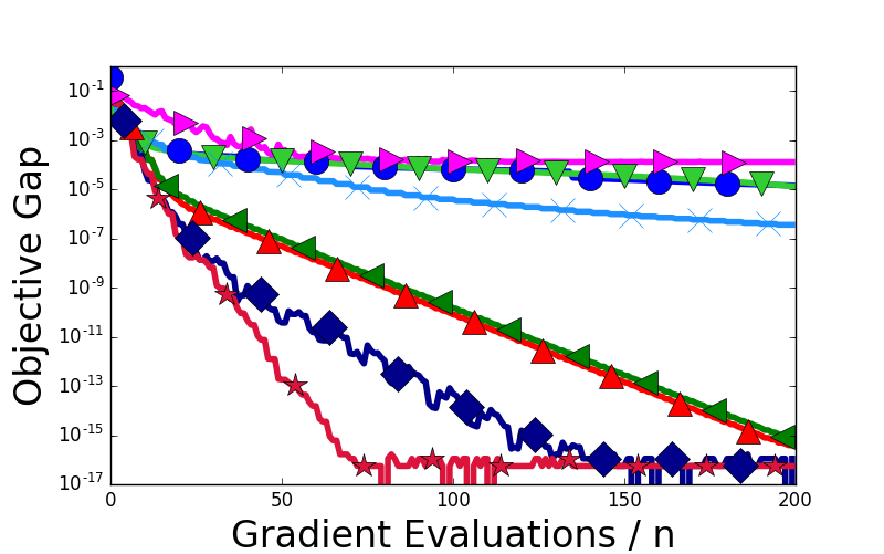
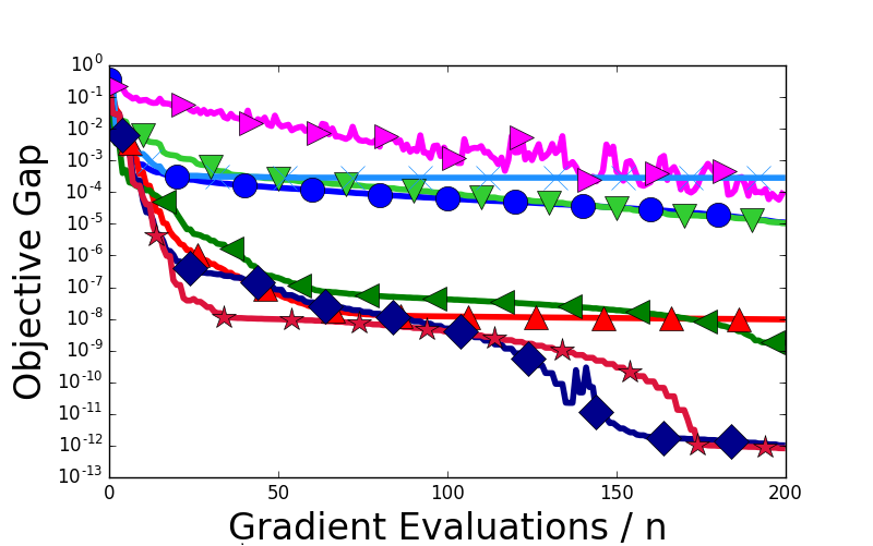
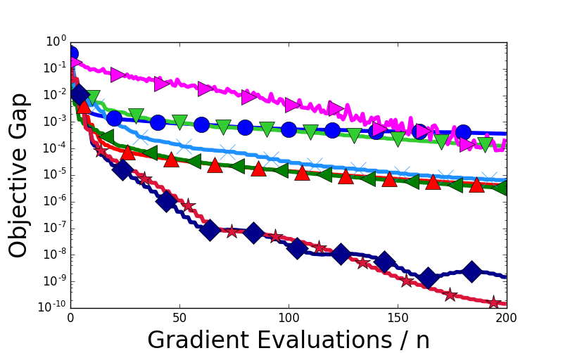
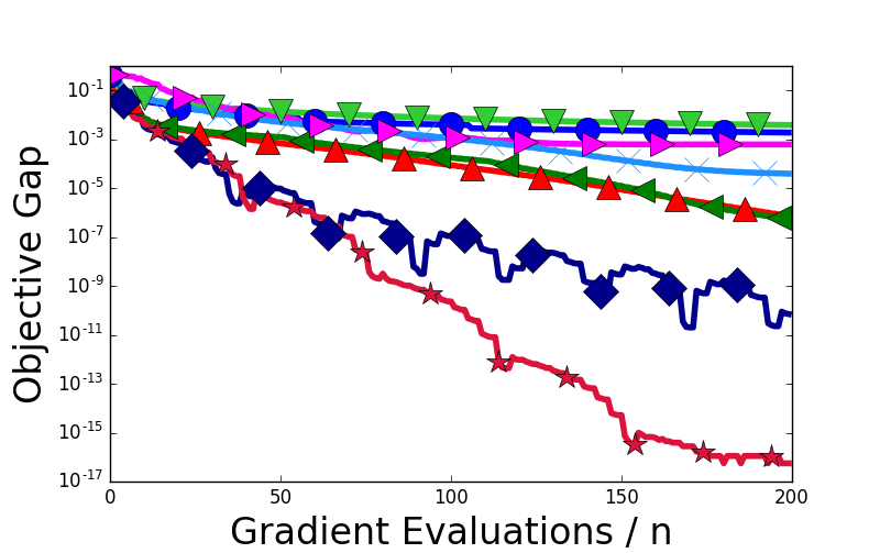
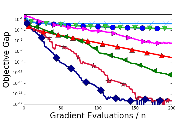
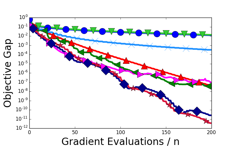
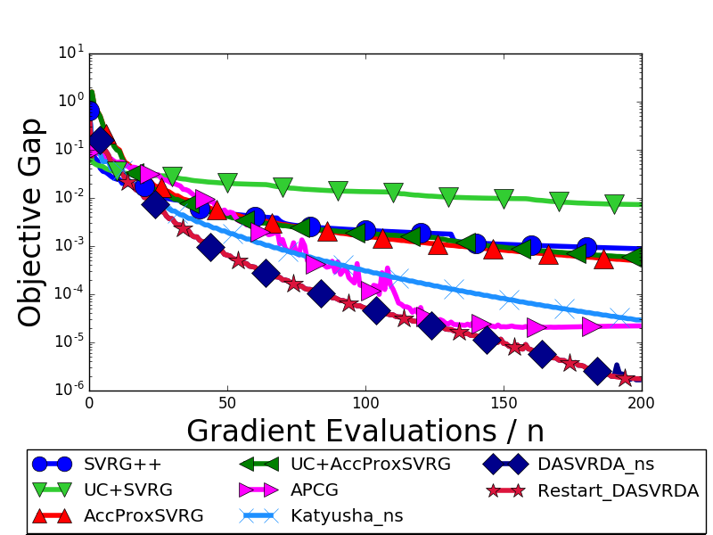
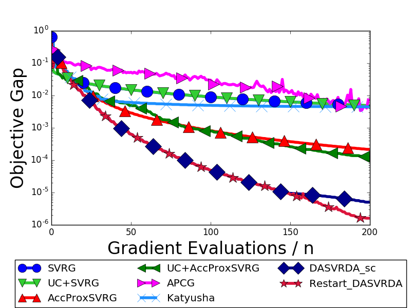
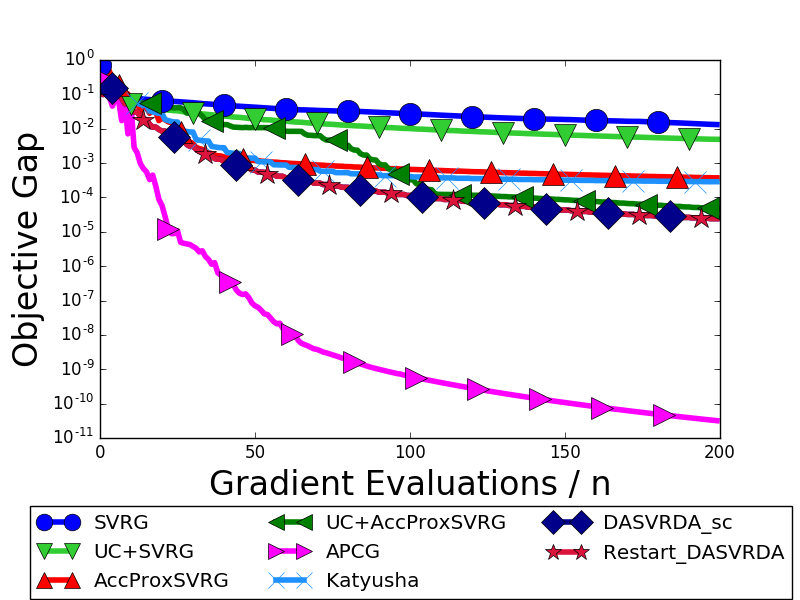
We numerically compare our method with several well-known stochastic gradient methods in mini-batch settings: SVRG (Xiao & Zhang, 2014) (and SVRG⁺⁺ (Allen-Zhu & Yuan, 2016)), AccProxSVRG (Nitanda, 2014), Universal Catalyst (Lin et al., 2015) , APCG (Lin et al., 2014a), and Katyusha (Allen-Zhu, 2016). The details of the implemented algorithms and their parameter tunings are found in the supplementary material. In the experiments, we focus on the regularized logistic regression problem for binary classification, with regularizer $\lambda_{1}\|\cdot\|_{1}+(\lambda_{2}/2)\|\cdot\|_{2}^{2}$.

We used three publicly available data sets in the experiments. Their sizes $n$ and dimensions $d$, and common min-batch sizes $b$ for all implemented algorithms are listed in Table 2.

Data sets	$n$	$d$	$b$
a9a	$32,561$	$123$	$180$
rcv1	$20,242$	$47,236$	$140$
sido0	$12,678$	$4,932$	$100$

T 2: Summary of the data sets and mini-batch size used in our numerical experiments

For regularization parameters, we used three settings $(\lambda_{1},\lambda_{2})=(10^{-4},0)$, $(10^{-4},10^{-6})$, and $(0,10^{-6})$. For the former case, the objective is non-strongly convex, and for the latter two cases, the objectives are strongly convex. Note that for the latter two cases, the strong convexity of the objectives is $\mu=10^{-6}$ and is relatively small; thus, it makes acceleration methods beneficial.

Figure 1 shows the comparisons of our method with the different methods described above on several settings. “Objective Gap” means $P(x)-P(x_{*})$ for the output solution $x$. “Gradient Evaluations $/n$” is the number of computations of stochastic gradients $\nabla f_{i}$ divided by $n$. “Restart$\textunderscore$DASVRDA” means DASVRDA with heuristic adaptive restarting. We can observe the following from these results:

• Our proposed DASVRDA and Restart$\textunderscore$DASVRDA significantly outperformed all the other methods overall.

• DASVRDA with the heuristic adaptive restart scheme efficiently made use of the local strong convexities of non-strongly convex objectives and significantly outperformed vanilla DASVRDA on a9a and rcv1 data sets. For the other settings, the algorithm was still comparable to vanilla DASVRDA.

• UC$+$SVRG did not work as well as it did in theory, and its performances were almost the same as that of vanilla SVRG.

• UC$+$AccProxSVRG sometimes outperformed vanilla AccProxSVRG but was always outperformed by our methods.

• APCG sometimes performed unstably and was outperformed by vanilla SVRG. On sido0 data set, for Elastic Net Setting, APCG significantly outperformed all other methods.

• Katyusha outperformed vanilla SVRG overall. However, sometimes Katyusha was slower than vanilla SVRG for Elastic Net Settings. This is probably because SVRG is almost adaptive to local strong convexities of loss functions, whereas Katyusha is not (see the remark in supplementary material).

8 Conclusion

In this paper, we developed a new accelerated stochastic variance reduced gradient method for regularized empirical risk minimization problems in mini-batch settings: DASVRDA. We have shown that DASVRDA achieves the total computational costs of $O(d(n\mathrm{log}(1/\varepsilon)+\sqrt{nL/\varepsilon}+b\sqrt{L/\varepsilon}))$ and $O(d(n+\sqrt{nL/\mu}+b\sqrt{L/\mu})\mathrm{log}(1/\varepsilon))$ in size $b$ mini-batch settings for non-strongly and strongly convex objectives, respectively. In addition, DASVRDA essentially achieves the optimal iteration complexities only with size $O(\sqrt{n})$ mini-batches for both settings. In the numerical experiments, our method significantly outperformed state-of-the-art methods, including Katyusha and AccProxSVRG.

In this supplementary material, we give the proofs of Theorem 5.1 and the optimality of $\gamma_{*}$ (Section A), Theorem 5.2 (Section B) and Corollary 5.3 (Section C), the lazy update algorithm of our method (Section D) and the experimental details (Section E). Finally, we briefly discuss DASVRG method, which is a variant of DASVRDA method (Section F).

Appendix A Proof of Theorem 5.1

In this section, we give the comprehensive proof of Theorem 5.1. First we analyze One Stage Accelerated SVRDA algorithm.

Lemma A.1.

The sequence $\{\theta_{k}\}_{k\geq 1}$ defined in Algorithm 7 satisfies

$$\theta_{k}-1=\theta_{k-2}$$

for $k\geq 1$, where $\theta_{-1}\overset{\mathrm{def}}{=}0$.

Proof.

Since $\theta_{k}=\frac{k+1}{2}$ for $k\geq 0$, we have that

$$\theta_{k}-1=\frac{k+1}{2}-1=\frac{k-1}{2}=\theta_{k-2}.$$

∎

Lemma A.2.

The sequence $\{\theta_{k}\}_{k\geq 1}$ defined in Algorithm 7 satisfies

$$\theta_{m}\theta_{m-1}=\sum_{k=1}^{m}\theta_{k-1}.$$

∎

Proof.

Observe that

$$\theta_{m}\theta_{m-1}=\frac{m(m+1)}{4}=\sum_{k=1}^{m}\frac{k}{2}=\sum_{k=1}^{m}\theta_{k-1}.$$

∎

Lemma A.3.

For every $x$, $y\in\mathbb{R}^{d}$,

$$F(y)+\langle\nabla F(y),x-y\rangle+R(x)\leq P(x)-\frac{1}{2\bar{L}}\frac{1}{n}\sum_{i=1}^{n}\frac{1}{nq_{i}}\|\nabla f_{i}(x)-\nabla f_{i}(y)\|^{2}.$$

Proof.

Since $f_{i}$ is convex and $L_{i}$-smooth, we have (see (Nesterov, 2013))

$$f_{i}(y)+\langle\nabla f_{i}(y),x-y\rangle\leq f_{i}(x)-\frac{1}{2L_{i}}\|\nabla f_{i}(x)-\nabla f_{i}(y)\|^{2}.$$

By the definition of $\{q_{i}\}$, summing this inequality from $i=1$ to $n$ and dividing it by $n$ results in

$$F(y)+\langle\nabla F(y),x-y\rangle\leq F(x)-\frac{1}{2\bar{L}}\frac{1}{n}\sum_{i=1}^{n}\frac{1}{nq_{i}}\|\nabla f_{i}(x)-\nabla f_{i}(y)\|^{2}.$$

Adding $R(x)$ to the both sides of this inequality gives the desired result. ∎

Lemma A.4.

$$\bar{g}_{k}=\frac{1}{\theta_{k}\theta_{k-1}}\sum_{k^{\prime}=1}^{k}\theta_{k^{\prime}-1}g_{k^{\prime}}\ (k\geq 1).$$

Proof.

For $k=1$, $\bar{g}_{1}=g_{1}=\frac{1}{1\cdot\frac{1}{2}}\sum_{k^{\prime}=1}^{1}\frac{1}{2}\cdot g_{k^{\prime}}$ by the definition of $\theta_{0}$.
Assume that the claim holds for some $k\geq 1$. Then

$$\bar{g}_{k+1}= \ \left(1-\frac{1}{\theta_{k+1}}\right)\bar{g}_{k}+\frac{1}{\theta_{k+1}}g_{k+1}$$

$$= \ \left(1-\frac{2}{k+2}\right)\frac{4}{(k+1)k}\sum_{k^{\prime}=1}^{k}\theta_{k^{\prime}-1}g_{k^{\prime}}+\frac{2}{k+2}g_{k+1}$$

$$= \ \frac{4}{(k+2)(k+1)}\sum_{k^{\prime}=1}^{k+1}\theta_{k^{\prime}-1}g_{k^{\prime}}$$

$$= \ \frac{1}{\theta_{k+1}\theta_{k}}\sum_{k^{\prime}=1}^{k+1}\theta_{k^{\prime}-1}g_{k^{\prime}}.$$

The first equality follows from the definition of $\bar{g}_{k+1}$. Second equality is due to the assumption of the induction. This finishes the proof for Lemma A.4. ∎

Next we prove the following main lemma for One Stage Accelerated SVRDA. The proof is inspired by the one of AccSDA given in (Xiao, 2009).

Lemma A.5.

Let $\eta<1/\bar{L}$. For One Stage Accelerated SVRDA, we have that

$$\mathbb{E}[P(x_{m})-P(x)]$$

$$\leq \ \frac{2}{\eta(m+1)m}\|z_{0}-x\|^{2}-\frac{2}{\eta(m+1)m}\mathbb{E}\|z_{m}-x\|^{2}$$

$$+\frac{2}{(m+1)m}\sum_{k=1}^{m}\left(\frac{(k+1)k\mathbb{E}\|g_{k}-\nabla F(y_{k})\|^{2}}{4\left(\frac{1}{\eta}-\bar{L}\right)}-\frac{k}{2\bar{L}}\frac{1}{n}\sum_{i=1}^{n}\frac{1}{nq_{i}}\mathbb{E}\|\nabla f_{i}(y_{k})-\nabla f_{i}(x)\|^{2}\right),$$

for any $x\in\mathbb{R}^{d}$, where the expectations are taken with respect to $I_{k}(1\leq k\leq m)$.

Proof.

We define

$$\ell_{k}(x) =F(y_{k})+\langle\nabla F(y_{k}),x-y_{k}\rangle+R(x),$$

$$\hat{\ell}_{k}(x) =F(y_{k})+\langle g_{k},x-y_{k}\rangle+R(x).$$

Observe that $\ell_{k},\hat{\ell}_{k}$ is convex and $\ell_{k}\leq P$ by the convexity of $F$ and $R$. Moreover, for $k\geq 1$ we have that

$$\sum_{k^{\prime}=1}^{k}\theta_{k^{\prime}-1}\hat{\ell}_{k^{\prime}}(z)= \sum_{k^{\prime}=1}^{k}\theta_{k^{\prime}-1}F(y_{k})+\sum_{k^{\prime}=1}^{k}\langle\theta_{k^{\prime}-1}g_{k^{\prime}},z-y_{k^{\prime}}\rangle+\sum_{k^{\prime}=1}^{k}\theta_{k^{\prime}-1}R(z)$$

$$= \left\langle\theta_{k}\theta_{k-1}\bar{g}_{k},z\right\rangle+\theta_{k}\theta_{k-1}R(z)+\sum_{k^{\prime}=1}^{k}\theta_{k^{\prime}-1}F(y_{k})-\sum_{k^{\prime}=1}^{k}\theta_{k^{\prime}-1}\langle g_{k^{\prime}},y_{k^{\prime}}\rangle.$$

The second equality follows from Lemma A.4 and Lemma A.2. Thus we see that $z_{k}=\underset{z\in\mathbb{R}^{d}}{\mathrm{argmin}\ }\left\{\sum_{k^{\prime}=1}^{k}\theta_{k^{\prime}-1}\hat{\ell}_{k^{\prime}}(z)+\frac{1}{2\eta}\|z-z_{0}\|^{2}\right\}$. Observe that $F$ is convex and $\bar{L}$-smooth. Thus we have that

$$F(x_{k})\leq F(y_{k})+\langle\nabla F(y_{k}),x_{k}-y_{k}\rangle+\frac{\bar{L}}{2}\|x_{k}-y_{k}\|^{2}.$$ (4)

Hence we see that

$$P(x_{k})\leq \ \ell_{k}(x_{k})+\frac{\bar{L}}{2}\|x_{k}-y_{k}\|^{2}$$

$$= \ \ell_{k}\left(\left(1-\frac{1}{\theta_{k}}\right)x_{k-1}+\frac{1}{\theta_{k}}z_{k}\right)+\frac{\bar{L}}{2}\left\|\left(1-\frac{1}{\theta_{k}}\right)x_{k-1}+\frac{1}{\theta_{k}}z_{k}-y_{k}\right\|^{2}$$

$$\leq \ \left(1-\frac{1}{\theta_{k}}\right)\ell_{k}(x_{k-1})+\frac{1}{\theta_{k}}\ell_{k}(z_{k})+\frac{\bar{L}}{2\theta_{k}^{2}}\|z_{k}-z_{k-1}\|^{2}$$

$$\leq \ \left(1-\frac{1}{\theta_{k}}\right)P(x_{k-1})+\frac{1}{\theta_{k}\theta_{k-1}}\left(\theta_{k-1}\hat{\ell}_{k}(z_{k})+\frac{\bar{L}}{2}\|z_{k}-z_{k-1}\|^{2}\right)$$

$$-\frac{1}{\theta_{k}}\langle g_{k}-\nabla F(y_{k}),z_{k}-y_{k}\rangle$$

$$= \ \left(1-\frac{1}{\theta_{k}}\right)P(x_{k-1})+\frac{1}{\theta_{k}\theta_{k-1}}\left(\theta_{k-1}\hat{\ell}_{k}(z_{k})+\frac{1}{2\eta}\|z_{k}-z_{k-1}\|^{2}\right)$$

$$-\frac{1}{2\theta_{k}\theta_{k-1}}\left(\frac{1}{\eta}-\bar{L}\right)\|z_{k}-z_{k-1}\|^{2}-\frac{1}{\theta_{k}}\langle g_{k}-\nabla F(y_{k}),z_{k}-z_{k-1}\rangle$$

$$-\frac{1}{\theta_{k}}\langle g_{k}-\nabla F(y_{k}),z_{k-1}-y_{k}\rangle.$$

The first inequality follows from (4). The first equality is due to the definition of $x_{k}$. The second inequality is due to the convexity of $\ell_{k}$ and the definition of $y_{k}$. The third inequality holds because $\ell_{k}\leq P$ and $\frac{1}{\theta_{k}^{2}}\leq\frac{1}{\theta_{k}\theta_{k-1}}$.

Since $\frac{1}{\eta}>\bar{L}$, we have that

$$- \frac{1}{2\theta_{k}\theta_{k-1}}\left(\frac{1}{\eta}-\bar{L}\right)\|z_{k}-z_{k-1}\|^{2}-\frac{1}{\theta_{k}}\langle g_{k}-\nabla F(y_{k}),z_{k}-z_{k-1}\rangle$$

$$\leq \frac{1}{\theta_{k}}\frac{\theta_{k-1}\|g_{k}-\nabla F(y_{k})\|^{2}}{2\left(\frac{1}{\eta}-\bar{L}\right)}$$

$$\leq \frac{\|g_{k}-\nabla F(y_{k})\|^{2}}{2\left(\frac{1}{\eta}-\bar{L}\right)}.$$

The first inequality is due to Young’s inequality. The second inequality holds because $\theta_{k-1}\leq\theta_{k}$.

Using this inequality, we get that

$$P(x_{k})\leq \ \left(1-\frac{1}{\theta_{k}}\right)P(x_{k-1})+\frac{1}{\theta_{k}\theta_{k-1}}\left(\theta_{k-1}\hat{\ell}_{k}(z_{k})+\frac{1}{2\eta}\|z_{k}-z_{k-1}\|^{2}\right)$$

$$+\frac{\|g_{k}-\nabla F(y_{k})\|^{2}}{2\left(\frac{1}{\eta}-\bar{L}\right)}-\frac{1}{\theta_{k}}\langle g_{k}-\nabla F(y_{k}),z_{k-1}-y_{k}\rangle.$$

Multiplying the both sides of the above inequality by $\theta_{k}\theta_{k-1}$ yields

$$\theta_{k}\theta_{k-1}P(x_{k})\leq \ \theta_{k-1}(\theta_{k}-1)P(x_{k-1})+\theta_{k-1}\hat{\ell}_{k}(z_{k})+\frac{1}{2\eta}\|z_{k}-z_{k-1}\|^{2}$$

$$+\frac{\theta_{k}\theta_{k-1}\|g_{k}-\nabla F(y_{k})\|^{2}}{2\left(\frac{1}{\eta}-\bar{L}\right)}-\theta_{k-1}\langle g_{k}-\nabla F(y_{k}),z_{k-1}-y_{k}\rangle.$$ (5)

By the fact that $\sum_{k^{\prime}=1}^{k-1}\theta_{k^{\prime}-1}\hat{\ell}_{k^{\prime}}(z)+\frac{1}{2\eta}\|z-z_{0}\|^{2}$ is $\frac{1}{\eta}$-strongly convex and $z_{k-1}$ is the minimizer of $\sum_{k^{\prime}=1}^{k-1}\theta_{k^{\prime}-1}\hat{\ell}_{k^{\prime}}(z)+\frac{1}{2\eta}\|z-z_{0}\|^{2}$ for $k\geq 2$, we have that

$$\sum_{k^{\prime}=1}^{k-1}\theta_{k^{\prime}-1}\hat{\ell}_{k^{\prime}}(z_{k-1})+\frac{1}{2\eta}\|z_{k-1}-z_{0}\|^{2}+\frac{1}{2\eta}\|z_{k}-z_{k-1}\|^{2}\leq\sum_{k^{\prime}=1}^{k-1}\theta_{k^{\prime}-1}\hat{\ell}_{k^{\prime}}(z_{k})+\frac{1}{2\eta}\|z_{k}-z_{0}\|^{2}$$

for $k\geq 1$ (and, for $k=1$, we define $\sum_{k^{\prime}=1}^{0}=0$).

Using this inequality, we obtain

$$\theta_{k}\theta_{k-1}P(x_{k})-\sum_{k^{\prime}=1}^{k}\theta_{k^{\prime}-1}\hat{\ell}_{k^{\prime}}(z_{k})-\frac{1}{2\eta}\|z_{k}-z_{0}\|^{2}$$

$$\leq \theta_{k-1}\theta_{k-2}P(x_{k-1})-\sum_{k^{\prime}=1}^{k-1}\theta_{k^{\prime}-1}\hat{\ell}_{k^{\prime}}(z_{k-1})-\frac{1}{2\eta}\|z_{k-1}-z_{0}\|^{2}+\frac{\theta_{k}\theta_{k-1}}{2\left(\frac{1}{\eta}-\bar{L}\right)}\|g_{k}-\nabla F(y_{k})\|^{2}$$

$$-\theta_{k-1}\langle g_{k}-\nabla F(y_{k}),z_{k-1}-y_{k}\rangle.$$

Here, the inequality follows from Lemma A.1 (we defined $\theta_{-1}\overset{\mathrm{def}}{=}0$).

Summing the above inequality from $k=1$ to $m$ results in

$$\theta_{m}\theta_{m-1}P(x_{m})-\sum_{k=1}^{m}\theta_{k-1}\hat{\ell}_{k}(z_{m})-\frac{1}{2\eta}\|z_{m}-z_{0}\|^{2}$$

$$\leq \ \sum_{k=1}^{m}\frac{\theta_{k}\theta_{k-1}\|g_{k}-\nabla F(y_{k})\|^{2}}{{2\left(\frac{1}{\eta}-\bar{L}\right)}}-\sum_{k=1}^{m}\theta_{k-1}\langle g_{k}-\nabla F(y_{k}),z_{k-1}-y_{k}\rangle.$$

Using $\frac{1}{\eta}$-strongly convexity of the function $\sum_{k=1}^{m}\theta_{k-1}\hat{\ell}_{k}(z)+\frac{1}{2\eta}\|z-z_{0}\|^{2}$ and the optimality of $z_{m}$, we have that

$$\sum_{k=1}^{m}\theta_{k-1}\hat{\ell}_{k}(z_{m})+\frac{1}{2\eta}\|z_{m}-z_{0}\|^{2}\leq\sum_{k=1}^{m}\theta_{k-1}\hat{\ell}_{k}(x)+\frac{1}{2\eta}\|z_{0}-x\|^{2}-\frac{1}{2\eta}\|z_{m}-x\|^{2}.$$

From this inequality, we see that

$$\theta_{m}\theta_{m-1}P(x_{m})$$

$$\leq \ \sum_{k=1}^{m}\theta_{k-1}\hat{\ell}_{k}(x)+\frac{1}{2\eta}\|z_{0}-x\|^{2}-\frac{1}{2\eta}\|z_{m}-x\|^{2}$$

$$+\sum_{k=1}^{m}\frac{\theta_{k}\theta_{k-1}\|g_{k}-\nabla F(y_{k})\|^{2}}{2\left(\frac{1}{\eta}-\bar{L}\right)}-\sum_{k=1}^{m}\theta_{k-1}\langle g_{k}-\nabla F(y_{k}),z_{k-1}-y_{k}\rangle$$

$$= \ \sum_{k=1}^{m}\theta_{k-1}\ell_{k}(x)+\frac{1}{2\eta}\|z_{0}-x\|^{2}-\frac{1}{2\eta}\|z_{m}-x\|^{2}$$

$$+\sum_{k=1}^{m}\frac{\theta_{k}\theta_{k-1}\|g_{k}-\nabla F(y_{k})\|^{2}}{2\left(\frac{1}{\eta}-\bar{L}\right)}-\sum_{k=1}^{m}\theta_{k-1}\langle g_{k}-\nabla F(y_{k}),z_{k-1}-x\rangle.$$

By Lemma A.3 with $x=x$ and $y=y_{k}$, we have that

$$\ell_{k}(x)\leq P(x)-\frac{1}{2\bar{L}}\frac{1}{n}\sum_{i=1}^{n}\frac{1}{nq_{i}}\|\nabla f_{i}(x)-\nabla f_{i}(y_{k})\|^{2}.$$

Applying this inequality to the above inequality yields

$$\theta_{m}\theta_{m-1}P(x_{m})-\sum_{k=1}^{m}\theta_{k-1}P(x)$$

$$\leq \ \frac{1}{2\eta}\|z_{0}-x\|^{2}-\frac{1}{2\eta}\|z_{m}-x\|^{2}$$

$$+\sum_{k=1}^{m}\left[\frac{\theta_{k}\theta_{k-1}\|g_{k}-\nabla F(y_{k})\|^{2}}{2\left(\frac{1}{\eta}-\bar{L}\right)}-\frac{\theta_{k-1}}{2\bar{L}}\frac{1}{n}\sum_{i=1}^{n}\frac{1}{nq_{i}}\|\nabla f_{i}(x)-\nabla f_{i}(y_{k})\|^{2}\right]$$

$$-\sum_{k=1}^{m}\theta_{k-1}\langle g_{k}-\nabla F(y_{k}),z_{k-1}-x\rangle.$$

Using Lemma A.2 and dividing the both sides of the above inequality by $\theta_{m}\theta_{m-1}$ result in

$$P(x_{m})-P(x)$$

$$\leq \frac{1}{2\eta\theta_{m}\theta_{m-1}}\|z_{0}-x\|^{2}-\frac{1}{2\eta\theta_{m}\theta_{m-1}}\|z_{m}-x\|^{2}$$

$$+\frac{1}{\theta_{m}\theta_{m-1}}\sum_{k=1}^{m}\left[\frac{\theta_{k}\theta_{k-1}\|g_{k}-\nabla F(y_{k})\|^{2}}{2\left(\frac{1}{\eta}-\bar{L}\right)}-\frac{\theta_{k-1}}{2\bar{L}}\frac{1}{n}\sum_{i=1}^{n}\frac{1}{nq_{i}}\|\nabla f_{i}(x)-\nabla f_{i}(y_{k})\|^{2}\right]$$

$$-\frac{1}{\theta_{m}\theta_{m-1}}\sum_{k=1}^{m}\theta_{k-1}\langle g_{k}-\nabla F(y_{k}),z_{k-1}-x\rangle.$$

Taking the expectations with respect to $I_{k}(1\leq k\leq m)$ on the both sides of this inequality yields

$$\mathbb{E}[P(x_{m})-P(x)]$$

$$\leq \frac{1}{2\eta\theta_{m}\theta_{m-1}}\|z_{0}-x\|^{2}-\frac{1}{2\eta\theta_{m}\theta_{m-1}}\mathbb{E}\|z_{m}-x\|^{2}$$

$$+\frac{1}{\theta_{m}\theta_{m-1}}\sum_{k=1}^{m}\left[\frac{\theta_{k}\theta_{k-1}\mathbb{E}\|g_{k}-\nabla F(y_{k})\|^{2}}{2\left(\frac{1}{\eta}-\bar{L}\right)}-\frac{\theta_{k-1}}{2\bar{L}}\frac{1}{n}\sum_{i=1}^{n}\frac{1}{nq_{i}}\mathbb{E}\|\nabla f_{i}(x)-\nabla f_{i}(y_{k})\|^{2}\right].$$

Here we used the fact that $\mathbb{E}[g_{k}-\nabla F(y_{k})]=0$ for $k=1,\ldots,m$. This finishes the proof of Lemma A.5. ∎

Now we need the following lemma.

Lemma A.6.

For every $x\in\mathbb{R}^{d}$,

$$\frac{1}{n}\sum_{i=1}^{n}\frac{1}{nq_{i}}\|\nabla f_{i}(x)-\nabla f_{i}(x_{*})\|^{2}\leq 2\bar{L}(P(x)-P(x_{*})).$$

Proof.

From the argument of the proof of Lemma A.3, we have

$$\frac{1}{n}\sum_{i=1}^{n}\frac{1}{nq_{i}}\|\nabla f_{i}(x)-\nabla f_{i}(x_{*})\|^{2}\leq 2\bar{L}(F(x)-\langle\nabla F(x_{*}),x-x_{*}\rangle-F(x_{*})).$$

By the optimality of $x_{*}$, there exists $\xi_{*}\in\partial R(x_{*})$ such that $\nabla F(x_{*})+\xi_{*}=0$. Then we have

$$-\langle\nabla F(x_{*}),x-x_{*}\rangle=\langle\xi_{*},x-x_{*}\rangle\leq R(x)-R(x_{*}),$$

and hence

$$\frac{1}{n}\sum_{i=1}^{n}\frac{1}{nq_{i}}\|\nabla f_{i}(x)-\nabla f_{i}(x_{*})\|^{2}\leq 2\bar{L}(P(x)-P(x_{*})).$$

∎

Proposition A.7.

Let $\gamma>1$ and $\eta\leq 1/((1+\gamma(m+1)/b)\bar{L})$. For One Pass Accelerated SVRDA, it follows that

$$\mathbb{E}[P(x_{m})-P(\widetilde{x})]\leq\frac{2}{\eta(m+1)m}\mathbb{\|}\widetilde{y}-\widetilde{x}\|^{2}-\frac{2}{\eta(m+1)m}\mathbb{E}\|z_{m}-\widetilde{x}\|^{2},$$

and

$$\mathbb{E}[P({x}_{m})-P(x_{*})]$$

$$\leq \ \frac{1}{\gamma}(P(\widetilde{x})-P(x_{*}))+\frac{2}{\eta(m+1)m}\|\widetilde{y}-x_{*}\|^{2}-\frac{2}{\eta(m+1)m}\mathbb{E}\|z_{m}-x_{*}\|^{2},$$

where the expectations are taken with respect to $I_{k}(1\leq k\leq m)$.

Proof.

We bound the variance of the averaged stochastic gradient $\mathbb{E}\|g_{k}-\nabla F(y_{k})\|^{2}$:

$$\mathbb{E}\|g_{k}-\nabla F(y_{k})\|^{2}$$

$$= \ \mathbb{E}\left[\mathbb{E}_{I_{k}}\|g_{k}-\nabla F(y_{k})\|^{2}\mid[k-1]\right]$$

$$= \ \frac{1}{b}\mathbb{E}\left[\mathbb{E}_{i\sim Q}\|(\nabla f_{i}(y_{k})-\nabla f_{i}(\widetilde{x}))/nq_{i}+\nabla F(\widetilde{x})-\nabla F(y_{k})\|^{2}\mid[k-1]\right]$$

$$\leq \ \frac{1}{b}\mathbb{E}\left[\mathbb{E}_{i\sim Q}\|(\nabla f_{i}(y_{k})-\nabla f_{i}(\widetilde{x}))/nq_{i}\|^{2}\mid[k-1]\right]$$

$$= \ \frac{1}{b}\mathbb{E}\left[\frac{1}{n}\sum_{i=1}^{n}\frac{1}{nq_{i}}\|\nabla f_{i}(y_{k})-\nabla f_{i}(\widetilde{x})\|^{2}\right]$$ (6)

$$\leq \ \frac{2}{b}\mathbb{E}\left[\frac{1}{n}\sum_{i=1}^{n}\frac{1}{nq_{i}}\|\nabla f_{i}(y_{k})-\nabla f_{i}(x_{*})\|^{2}\right]$$

$$+\frac{2}{b}\mathbb{E}\left[\frac{1}{n}\sum_{i=1}^{n}\frac{1}{nq_{i}}\|\nabla f_{i}(\widetilde{x})-\nabla f_{i}(x_{*})\|^{2}\right]$$

$$\leq \ \frac{2}{b}\mathbb{E}\left[\frac{1}{n}\sum_{i=1}^{n}\frac{1}{nq_{i}}\|\nabla f_{i}(y_{k})-\nabla f_{i}(x_{*})\|^{2}\right]+\frac{4\bar{L}}{b}(P(\widetilde{x})-P(x_{*})).$$ (7)

The second equality follows from the independency of the random variables $\{i_{1},\ldots,i_{b}\}$ and the unbiasedness of $(\nabla f_{i}(y_{k})-\nabla f_{i}(\widetilde{x}))/nq_{i}+\nabla F(\widetilde{x})$. The first inequality is due to the fact that $\mathbb{E}\|X-\mathbb{E}[X]\|^{2}\leq\mathbb{E}\|X\|^{2}$. The second inequality follows from Young’s inequality. The final inequality is due to Lemma A.6.

Since $\frac{1}{\eta}\geq\left(1+\frac{\gamma(m+1)}{b}\right)\bar{L}$ and $\gamma>1$, using (6) yields

$$\frac{(k+1)k}{4\left(\frac{1}{\eta}-\bar{L}\right)}\mathbb{E}\|g_{k}-\nabla F(y_{k})\|^{2}-\frac{k}{2\bar{L}}\mathbb{E}\left[\frac{1}{n}\sum_{i=1}^{n}\frac{1}{nq_{i}}\|\nabla f_{i}(y_{k})-\nabla f_{i}(\widetilde{x})\|^{2}\right]\leq 0.$$

By Lemma A.5 (with $x=\widetilde{x}$) we have

$$\mathbb{E}[P(x_{m})-P(\widetilde{x})]\leq\frac{2}{\eta(m+1)m}\mathbb{\|}\widetilde{y}-\widetilde{x}\|^{2}-\frac{2}{\eta(m+1)m}\mathbb{E}\|z_{m}-\widetilde{x}\|^{2}.$$

Similarly, combining Lemma A.5 (with $x=x_{*}$) with (7) results in

$$\mathbb{E}[P({x}_{m})-P(x_{*})]$$

$$\leq \ \frac{1}{\gamma}(P(\widetilde{x})-P(x_{*}))+\frac{2}{\eta(m+1)m}\|\widetilde{y}-x_{*}\|^{2}-\frac{2}{\eta(m+1)m}\mathbb{E}\|z_{m}-x_{*}\|^{2}.$$

These are the desired results. ∎

Lemma A.8.

The sequence $\{\widetilde{\theta}_{s}\}_{s\geq 1}$ defined in Algorithm 6 satisfies

$$\widetilde{\theta}_{s}\left(\widetilde{\theta}_{s}-1+\frac{1}{\gamma}\right)\leq\widetilde{\theta}_{s-1}^{2}$$

for any $s\geq 1$.

Proof.

Since $\widetilde{\theta}_{s}=\left(1-\frac{1}{\gamma}\right)\frac{s+2}{2}$ for $s\geq 0$, we have

$$\widetilde{\theta}_{s}\left(\widetilde{\theta}_{s}-1+\frac{1}{\gamma}\right)$$

$$= \ \left(1-\frac{1}{\gamma}\right)\frac{s+2}{2}\left(\left(1-\frac{1}{\gamma}\right)\frac{s+2}{2}-1+\frac{1}{\gamma}\right)$$

$$= \ \left(1-\frac{1}{\gamma}\right)^{2}\frac{s(s+2)}{4}$$

$$\leq \ \widetilde{\theta}_{s-1}^{2}.$$

This finishes the proof of Lemma A.8. ∎

Now we are ready to proof Theorem 5.1.

Proof of Theorem 5.1.

By Proposition A.7, we have

$$\mathbb{E}[P(\widetilde{x}_{s})-P(\widetilde{x}_{s-1})]\leq\frac{2}{\eta(m+1)m}\mathbb{E}\|\widetilde{y}_{s}-\widetilde{x}_{s-1}\|^{2}-\frac{2}{\eta(m+1)m}\mathbb{E}\|\widetilde{z}_{s}-\widetilde{x}_{s-1}\|^{2},$$

and

$$\mathbb{E}[P(\widetilde{x}_{s})-P(x_{*})]$$

$$\leq \ \frac{1}{\gamma}\mathbb{E}[P(\widetilde{x}_{s-1})-P(x_{*})]+\frac{2}{\eta(m+1)m}\mathbb{E}\|\widetilde{y}_{s}-x_{*}\|^{2}-\frac{2}{\eta(m+1)m}\mathbb{E}\|\widetilde{z}_{s}-x_{*}\|^{2},$$

where the expectations are taken with respect to the history of all random variables.

Hence we have

$$\mathbb{E}[P(\widetilde{x}_{s})-P(\widetilde{x}_{s-1})]\leq\frac{4}{\eta(m+1)m}\mathbb{E}\langle\widetilde{z}_{s}-\widetilde{y}_{s},\widetilde{x}_{s-1}-\widetilde{y}_{s}\rangle-\frac{2}{\eta(m+1)m}\mathbb{E}\|\tilde{z}_{s}-\tilde{y}_{s}\|^{2},$$ (8)

and

$$\mathbb{E}[P(\widetilde{x}_{s})-P(x_{*})]$$

$$\leq \ \frac{1}{\gamma}\mathbb{E}[P(\widetilde{x}_{s-1})-P(x_{*})]+\frac{4}{\eta(m+1)m}\mathbb{E}\langle\widetilde{z}_{s}-\widetilde{y}_{s},x_{*}-\widetilde{y}_{s}\rangle-\frac{2}{\eta(m+1)m}\mathbb{E}\|\widetilde{z}_{s}-\widetilde{y}_{s}\|^{2}.$$ (9)

Since $\gamma\geq 3$, we have $\widetilde{\theta}_{s}\geq 1$ for $s\geq 1$. Multiplying (8) by $\widetilde{\theta}_{s}(\widetilde{\theta}_{s}-1)\geq 0$ and adding $\widetilde{\theta}_{s}\times$ (9) yield

$$\widetilde{\theta}_{s}^{2}\mathbb{E}[P(\widetilde{x}_{s})-P(x_{*})]-\widetilde{\theta}_{s}\left(\widetilde{\theta}_{s}-1+\frac{1}{\gamma}\right)\mathbb{E}[P(\widetilde{x}_{s-1})-P(x_{*})]$$

$$\leq \ \frac{4}{\eta(m+1)m}\mathbb{E}\langle\widetilde{\theta}_{s}(\widetilde{z}_{s}-\widetilde{y}_{s}),(\widetilde{\theta}_{s}-1)\widetilde{x}_{s-1}-\widetilde{\theta}_{s}\widetilde{y}_{s}+x_{*}\rangle-\frac{2}{\eta(m+1)m}\mathbb{E}\|\widetilde{\theta}_{s}(\widetilde{z}_{s}-\widetilde{y}_{s})\|^{2}.$$

By Lemma (A.8), we have

$$\widetilde{\theta}_{s}\left(\widetilde{\theta}_{s}-1+\frac{1}{\gamma}\right)\leq\widetilde{\theta}_{s-1}^{2}$$

for $s\geq 1$.

Thus we get

$$\widetilde{\theta}_{s}^{2}\mathbb{E}[P(\widetilde{x}_{s})-P(x_{*})]-\widetilde{\theta}_{s-1}^{2}\mathbb{E}[P(\widetilde{x}_{s-1})-P(x_{*})]$$

$$\leq \ \frac{4}{\eta(m+1)m}\mathbb{E}\langle\widetilde{\theta}_{s}(\widetilde{z}_{s}-\widetilde{y}_{s}),(\widetilde{\theta}_{s}-1)\widetilde{x}_{s-1}-\widetilde{\theta}_{s}\widetilde{y}_{s}+x_{*}\rangle-\frac{2}{\eta(m+1)m}\mathbb{E}\|\widetilde{\theta}_{s}(\widetilde{z}_{s}-\widetilde{y}_{s})\|^{2}.$$

$$= \ \frac{2}{\eta(m+1)m}\left(\mathbb{E}\|(\widetilde{\theta}_{s}-1)\widetilde{x}_{s-1}-\widetilde{\theta}_{s}\widetilde{y}_{s}+x_{*}\|^{2}-\mathbb{E}\|(\widetilde{\theta}_{s}-1)\widetilde{x}_{s-1}-\widetilde{\theta}_{s}\widetilde{z}_{s}+x_{*}\|^{2}\right)$$

Since $\widetilde{y}_{s}=\widetilde{x}_{s-1}+\frac{\widetilde{\theta}_{s-1}-1}{\widetilde{\theta}_{s}}(\widetilde{x}_{s-1}-\widetilde{x}_{s-2})+\frac{\widetilde{\theta}_{s-1}}{\widetilde{\theta}_{s}}(\widetilde{z}_{s-1}-\widetilde{x}_{s-1})$, we have

$$(\widetilde{\theta}_{s}-1)\widetilde{x}_{s-1}-\widetilde{\theta}_{s}\widetilde{y}_{s}+x_{*}=(\widetilde{\theta}_{s-1}-1)\widetilde{x}_{s-2}-\widetilde{\theta}_{s-1}\widetilde{z}_{s-1}+x_{*}.$$

Therefore summing the above inequality from $s=1$ to $S$, we obtain

$$\widetilde{\theta}_{s}^{2}\mathbb{E}[P(\widetilde{x}_{S})-P(x_{*})]$$

$$\leq \ \widetilde{\theta}_{0}^{2}(P(\widetilde{x}_{0})-P(x_{*}))+\frac{2}{\eta(m+1)m}\|(\widetilde{\theta}_{0}-1)\widetilde{x}_{-1}-\widetilde{\theta}_{0}\widetilde{z}_{0}+x_{*}\|^{2}$$

$$= \ \left(1-\frac{1}{\gamma}\right)^{2}(P(\widetilde{x}_{0})-P(x_{*}))+\frac{2}{\eta(m+1)m}\|\widetilde{z}_{0}-x_{*}\|^{2}.$$

Dividing both sides by $\widetilde{\theta}_{s}^{2}$ finishes the proof of Theorem 5.1. ∎

Optimal choice of $\gamma$

We can choose the optimal value of $\gamma$ based on the following lemma.

Lemma A.9.

Define $g(\gamma)\overset{\mathrm{def}}{=}\frac{\left(1+\frac{\gamma(m+1)}{b}\right)}{\left(1-\frac{1}{\gamma}\right)^{2}}$ for $\gamma>1$. Then,

$$\gamma_{*}\overset{\mathrm{def}}{=}\underset{\gamma>1}{\mathrm{argmin}}\ g(\gamma)=\frac{1}{2}\left(3+\sqrt{9+\frac{8b}{m+1}}\right).$$

Proof.

First observe that

$$g^{\prime}(\gamma)=\frac{\frac{m+1}{b}\left(1-\frac{1}{\gamma}\right)^{2}-2\left(1+\frac{\gamma(m+1)}{b}\right)\left(1-\frac{1}{\gamma}\right)\frac{1}{\gamma^{2}}}{\left(1-\frac{1}{\gamma}\right)^{2}}.$$

Hence we have

$$g^{\prime}(\gamma)=0$$

$$\iff \frac{m+1}{b}\left(1-\frac{1}{\gamma}\right)^{2}-2\left(1+\frac{\gamma(m+1)}{b}\right)\left(1-\frac{1}{\gamma}\right)\frac{1}{\gamma^{2}}=0$$

$$\iff \frac{m+1}{b}(\gamma^{2}-\gamma)-2\left(1+\frac{\gamma(m+1)}{b}\right)=0$$

$$\iff \gamma^{2}-3\gamma-\frac{2b}{m+1}=0$$

$$\iff \gamma=\frac{1}{2}\left(3+\sqrt{9+\frac{8b}{m+1}}\right)=\gamma_{*}.$$

Here the second and last equivalencies hold from $\gamma>1$. Moreover observe that $g^{\prime}(\gamma)>0$ for $\gamma>\gamma_{*}$ and $g^{\prime}(\gamma)<0$ for $1<\gamma<\gamma_{*}$. This means that $\gamma_{*}$ is the minimizer of $g$ on the region $\gamma>1$. ∎

Appendix B Proof of Theorem 5.2

In this section, we give a proof of Theorem 5.2.

Proof of Theorem 5.2.

Since $\eta=1/((1+\gamma(m_{U}^{\prime}+1)/b)\bar{L})\leq 1/((1+\gamma(m_{u}+1)/b)\bar{L})$, from Proposition A.7, we have

$$\mathbb{E}[P(\widetilde{x}_{u})-P(x_{*})]+\frac{2}{\eta(m_{u}+1)m_{u}}\mathbb{E}\|\widetilde{z}_{u}-x_{*}\|^{2}$$

$$\leq \ \frac{1}{\gamma}(P(\widetilde{x}_{u-1})-P(x_{*}))+\frac{2}{\eta(m_{u}+1)m_{u}}\|\widetilde{z}_{u-1}-x_{*}\|^{2}$$

$$= \ \frac{1}{\gamma}\left(P(\widetilde{x}_{u-1})-P(x_{*})+\frac{2\gamma}{\eta(m_{u}+1)m_{u}}\|\widetilde{z}_{u-1}-x_{*}\|^{2}\right).$$

Since $m_{u}=\lceil\sqrt{\gamma(m_{u-1}+1)m_{u-1}}\rceil$, we have

$$\frac{2\gamma}{\eta(m_{u}+1)m_{u}}\leq\frac{2}{\eta(m_{u-1}+1)m_{u-1}}.$$

Using this inequality, we obtain that

$$\mathbb{E}[P(\widetilde{x}_{U})-P(x_{*})]+\frac{2}{\eta(m_{U}+1)m_{U}}\mathbb{E}\|\widetilde{z}_{U}-x_{*}\|^{2}$$

$$\leq \ \frac{1}{\gamma}\left(P(\widetilde{x}_{U-1})-P(x_{*})+\frac{2}{\eta(m_{U-1}+1)m_{U-1}}\mathbb{E}\|\widetilde{z}_{U-1}-x_{*}\|^{2}\right)$$

$$\leq \ \cdots$$

$$\leq \ \frac{1}{\gamma^{U}}\left(P(\widetilde{x}_{0})-P(x_{*})+\frac{2}{\eta(m_{0}+1)m_{0}}\|\widetilde{z}_{0}-x_{*}\|^{2}\right)$$

$$\leq \ \frac{1}{\gamma^{U}}\left(P(\widetilde{x}_{0})-P(x_{*})+\frac{2}{\eta(m_{0}+1)m_{0}}\|\widetilde{x}_{0}-x_{*}\|^{2}\right)$$

$$= \ O\left(\frac{1}{\gamma^{U}}(P(\widetilde{x}_{0})-P(x_{*}))\right).$$

The last equality is due to the definitions of $m_{0}$ and $\eta$, and the fact $m_{U}^{\prime}=O(m_{U})=O(\sqrt{\gamma}^{U}m_{0})=O(m)$ (see the arguments in the proof of Corollary 5.3). Since

$$\left(1-\frac{1}{\gamma}\right)^{2}(m_{U}^{\prime}+1)m_{U}^{\prime}\geq(m_{U}+1)m_{U},$$

we get

$$\mathbb{E}[P(\widetilde{x}_{U})-P(x_{*})]+\frac{2}{\left(1-\frac{1}{\gamma}\right)^{2}\eta(m_{U}^{\prime}+1)m_{U}^{\prime}}\mathbb{E}\|\widetilde{z}_{U}-x_{*}\|^{2}$$

$$\leq \ O\left(\frac{1}{\gamma^{U}}\left(P(\widetilde{x}_{0})-P(x_{*})\right)\right).$$

Using the definitions of $U$ and $m_{0}$ and combining this inequality with Theorem 5.1, we obtain that desired result. ∎

Appendix C Proof of Corollary 5.3

In this section, we give a proof of Corollary 5.3.

Proof of Corollary 5.3.

Observe that the total computational cost at the warm start phase becomes

$$O\left(dnU+db\sum_{u=1}^{U}m_{u}\right).$$

Since $m_{u}\leq\sqrt{\gamma}m_{u-1}+\sqrt{\gamma}+1\leq\sqrt{\gamma}m_{u-1}+2\sqrt{\gamma}\leq\sqrt{\gamma}^{2}m_{u-2}+2\sqrt{\gamma}+2\sqrt{\gamma}^{2}\leq\cdots\leq\sqrt{\gamma}^{u}m_{0}+2\sum_{u^{\prime}=1}^{u}\sqrt{\gamma}^{u^{\prime}}=O(\sqrt{\gamma}^{u}m_{0})$, we have

$$O\left(dnU+db\sum_{u=1}^{U}m_{u}\right)=O\left(dnU+db\sqrt{\gamma}^{U}m_{0}\right).$$

Suppose that $m\geq m_{0}\sqrt{(P(\widetilde{x}_{0})-P(x_{*}))/\varepsilon}$. Then, this condition implies $U=\lceil\mathrm{log}_{\sqrt{\gamma}}(m/m_{0})\rceil\geq\mathrm{log}_{\gamma}((P(\widetilde{x}_{0})-P(x_{*}))/\varepsilon)$. Hence we only need to run $u=O(\mathrm{log}_{\gamma}((P(\widetilde{x}_{0})-P(x_{*}))/\varepsilon))\leq U$ iterations at the warm start phase and running DASVRDA^ns is not needed. Then the total computational cost becomes

$$O\left(d\left(n\mathrm{log}\frac{P(\widetilde{x}_{0})-P(x_{*})}{\varepsilon}+bm_{0}\sqrt{\frac{P(\widetilde{x_{0}})-P(x_{*})}{\varepsilon}}\right)\right)\leq O\left(d\left(n\mathrm{log}\frac{P(\widetilde{x}_{0})-P(x_{*})}{\varepsilon}\right)\right),$$

here we used $mb=O(n)$. Next, suppose that $m\leq m_{0}\sqrt{(P(\widetilde{x}_{0})-P(x_{*}))/\varepsilon}$. In this case, the total computational cost at the warm start phase with full U iterations becomes

$$O\left(d\left(n\mathrm{log}\frac{m}{m_{0}}+mb\right)\right)\leq O\left(d\left(n\mathrm{log}\frac{P(\widetilde{x}_{0})-P(x_{*})}{\varepsilon}\right)\right).$$

Finally, using Theorem 5.2 yields the desired total computational cost. ∎

Appendix D Lazy Update Algorithm of DASVRDA Method

In this section, we discuss how to efficiently compute the updates of the DASVRDA algorithm for sparse data. Specifically, we derive lazy update rules of One Stage Accelerated SVRDA for the following empirical risk minimization problem:

$$\frac{1}{n}\sum_{i=1}^{n}\psi_{i}(a_{i}^{\top}x)+\lambda_{1}\|x\|_{1}+\frac{\lambda_{2}}{2}\|x\|_{2}^{2},\ \ \ \ \lambda_{1},\lambda_{2}\geq 0$$

For the sake of simplicity, we define the one dimensional soft-thresholding operator as follows:

$$\mathrm{soft}(z,\lambda)\overset{\mathrm{def}}{=}\mathrm{sign}\left(z\right)\mathrm{max}\{\left|z\right|-\lambda,0\},$$

for $z\in\mathbb{R}$. Moreover, in this section, we denote $[z_{1},z_{2}]$ as $\{z\in\mathbb{Z}\mid z_{1}\leq z\leq z_{2}\}$ for integers $z_{1},z_{2}\in\mathbb{Z}$. The explicit algorithm of the lazy updates for One Stage Accelerated SVRDA is given by Algorithm 10. Let us analyze the iteration cost of the algorithm. Suppose that each feature vector $a_{i}$ is sparse and the expected number of the nonzero elements is $O(d^{\prime})$. First note that $|\mathcal{A}_{k}|=O(bd^{\prime})$ expectedly if $d^{\prime}\ll d$. For updating $x_{k-1}$, by Proposition D.1, we need to compute $\sum_{k^{\prime}\in K_{j}^{\pm}}\theta_{k^{\prime}-2}/(1+\eta\theta_{k^{\prime}-1}\theta_{k^{\prime}-2}\lambda_{2})$ and $\sum_{k^{\prime}\in K_{j}^{\pm}}\theta_{k^{\prime}-1}\theta_{k^{\prime}-2}^{2}/(1+\eta\theta_{k^{\prime}-1}\theta_{k^{\prime}-2}\lambda_{2})$ for each $j\in\mathcal{A}_{k}$. For this, we first make lists $\{S_{k}\}_{k=1}^{m}=\{\sum_{k^{\prime}=1}^{k}\theta_{k^{\prime}-2}/(1+\eta\theta_{k^{\prime}-1}\theta_{k^{\prime}-2}\lambda_{2})\}_{k=1}^{m}$ and $\{S_{k}^{\prime}\}_{k=1}^{m}=\{\sum_{k^{\prime}=1}^{k}\theta_{k^{\prime}-1}\theta_{k^{\prime}-2}^{2}/(1+\eta\theta_{k^{\prime}-1}\theta_{k^{\prime}-2}\lambda_{2})\}_{k=1}^{m}$ before running the algorithm. This needs only $O(m)$. Note that these lists are not depend on coordinate $j$. Since $K_{j}^{\pm}$ are sets of continuous integers in $[k_{j}+2,k]$ or unions of two sets of continuous integers in $[k_{j}+2,k]$, we can efficiently compute the above sums. For example, if $K_{j}^{+}=[k_{j}+2,s_{-}]\cup[s_{+},k]$ for some integers $s_{\pm}\in[k_{j}+2,k]$, we can compute $\sum_{k^{\prime}\in K_{j}^{+}}\theta_{k^{\prime}-2}/(1+\eta\theta_{k^{\prime}-1}\theta_{k^{\prime}-2}\lambda_{2})$ as $S_{s_{-}}-S_{k_{j}+1}+S_{k}-S_{s_{+}-1}$ and this costs only $O(1)$. Thus, for computing $x_{k-1}$ and $y_{k}$, we need only $O(bd^{\prime})$ computational cost. For computing $g_{k}$, we need to compute the inner product $a_{i}^{\top}y_{k}$ for each $i\in I_{k}$ and this costs $O(bd^{\prime})$ expectedly. The expected cost of the rest of the updates is apparently $O(bd^{\prime})$. Hence, the total expected iteration cost of our algorithm in serial settings becomes $O(bd^{\prime})$ rather than $O(bd)$. Furthermore, we can extend our algorithm to parallel computing settings. Indeed, if we have $b$ processors, processor $b^{\prime}$ runs on the set $\mathcal{A}_{k}^{b^{\prime}}\overset{\mathrm{def}}{=}\{j\in[d]\mid a_{i_{b^{\prime}},j}\neq 0\}$. Then the total iteration cost per processor becomes ideally $O(d^{\prime})$. Generally the overlap among the sets $\mathcal{A}_{k}^{b^{\prime}}$ may cause latency, however for sufficiently sparse data, this latency is negligible. The following proposition guarantees that Algorithm 10 is equivalent to Algorithm 7 when $R(x)=\lambda_{1}\|x\|_{1}+(\lambda_{2}/2)\|x\|_{2}^{2}$.

Algorithm 10 Lazy Updates for One Stage AccSVRDA $(\widetilde{y},\widetilde{x},\eta,m,b,Q)$

0:  $\widetilde{y},\widetilde{x}$, $\eta>0$, $m\in\mathbb{N}$, $b\in[n]$, $Q$.

  $x_{0}=z_{0}=\widetilde{y}$.

  $g_{0,j}^{\mathrm{sum}}=0\ (j\in[d])$.

  $\theta_{0}=\frac{1}{2}$.

  $k_{j}=0\ \ (j\in[d])$.

  $\widetilde{\nabla}=\nabla F(\widetilde{x})$.

  for $k=1$ to $m$ do

     Sample independently $i_{1},\ldots,i_{b}\sim Q$. $I_{k}=\{i_{1},\ldots,i_{b}\}$.

     $\mathcal{A}_{k}=\{j\in[d]\mid\exists b^{\prime}\in[b]:a_{i_{b^{\prime}},j}\neq 0\}.$

     $\theta_{k}=\frac{k+1}{2}.$

     for $j\in\mathcal{A}_{k}$ do

         Update $x_{k-1,j}$, $y_{k,j}$ as in Proposition D.1.

     end for

     for $j\in\mathcal{A}_{k}$ do

        $g_{k,j}=\frac{1}{b}\sum_{i\in I_{t}}\frac{1}{nq_{i}}\left(\psi_{i}^{\prime}(a_{i}^{\top}y_{k})a_{i,j}-\psi_{i}^{\prime}(a_{i}^{\top}\widetilde{x})a_{i,j}\right)+\widetilde{\nabla}_{j}.$

        ${g}_{k,j}^{\mathrm{sum}}={g}_{k_{j},j}^{\mathrm{sum}}+\theta_{k-1}g_{k,j}+\left(\theta_{k}\theta_{k-1}-\theta_{k_{j}}\theta_{k_{j}-1}\right)\widetilde{\nabla}_{j}.$

        $z_{k,j}=\frac{1}{1+\eta\theta_{k}\theta_{k-1}\lambda_{2}}\mathrm{soft}(z_{0,j}-\eta g_{k,j}^{\mathrm{sum}},\eta\theta_{k}\theta_{k-1}\lambda_{1}).$

        $x_{k,j}=\left(1-\frac{1}{\theta_{k}}\right)x_{k-1,j}+\frac{1}{\theta_{k}}z_{k,j}.$

        $k_{j}=k.$

     end for

  end for

  $(x_{m},z_{m})$.

Proposition D.1.

Suppose that $R(x)=\lambda_{1}\|x\|_{1}+\frac{\lambda_{2}}{2}\|x\|_{2}^{2}$ with $\lambda_{1},\lambda_{2}\geq 0$. Let $j\in[d]$, $k_{j}\in[m]\cup\{0\}$ and $k\geq k_{j}+1$. Assume that $\nabla_{j}f_{i}(y_{k^{\prime}})=\nabla_{j}f_{i}(\widetilde{x})=0$ for any $i\in[b]$ and $k^{\prime}\in[k_{j}+1,k-1]$. In Algorithm 7, the following results hold:

$$x_{k-1,j}= \ \begin{cases}x_{0,j}\hskip 268.00043pt(k=1)\\ \frac{\theta_{k_{j}}\theta_{k_{j}-1}}{\theta_{k-1}\theta_{k-2}}x_{k_{j},j}+\frac{1}{\theta_{k-1}\theta_{k-2}}\sum_{k^{\prime}\in K_{j}^{+}}\frac{\theta_{k^{\prime}-2}}{1+\eta\theta_{k^{\prime}-1}\theta_{k^{\prime}-2}\lambda_{2}}(z_{0,j}-M_{k^{\prime},j}^{+})\hskip 16.00008pt(k\geq 2)\\ \hskip 59.00002pt+\ \frac{1}{\theta_{k-1}\theta_{k-2}}\sum_{k^{\prime}\in K_{j}^{-}}\frac{\theta_{k^{\prime}-2}}{1+\eta\theta_{k^{\prime}-1}\theta_{k^{\prime}-2}\lambda_{2}}(z_{0,j}-M_{k^{\prime},j}^{-})\end{cases},$$

$$y_{k,j}= \ \begin{cases}x_{0,j}\hskip 268.00043pt(k=1)\\ \left(1-\frac{1}{\theta_{k}}\right)x_{k-1,j}+\frac{1}{\theta_{k}}\frac{1}{1+\eta\theta_{k-1}\theta_{k-2}\lambda_{2}}\times\ \ \ \ \hskip 111.5001pt(k\geq 2)\\ \hskip 10.00002pt\mathrm{soft}\left(z_{0,j}-\eta g_{k_{j},j}^{\mathrm{sum}}-\eta(\theta_{k-1}\theta_{k-2}-\theta_{k_{j}}\theta_{k_{j}-1})\widetilde{\nabla}_{j},\eta\theta_{k-1}\theta_{k-2}\lambda_{1}\right)\end{cases},$$

and

$$z_{k,j}=\frac{1}{1+\eta\theta_{k}\theta_{k-1}\lambda_{2}}\mathrm{soft}(z_{0,j}-\eta g_{k,j}^{\mathrm{sum}},\eta\theta_{k}\theta_{k-1}\lambda_{1}),$$

where

$$M_{k^{\prime},j}^{\pm}\overset{\mathrm{def}}{=}\eta\theta_{k^{\prime}-1}\theta_{k^{\prime}-2}(\widetilde{\nabla}_{j}\pm\lambda_{1})+\eta g_{k_{j},j}^{\mathrm{sum}}-\eta\theta_{k_{j}}\theta_{k_{j}-1}\widetilde{\nabla}_{j},$$

and $K_{j}^{\pm}\subset[k_{j}+2,k]$ are defined as follows:
Let $c_{1}\overset{\mathrm{def}}{=}\frac{\eta\widetilde{\nabla}_{j}}{4}$, $c_{2}\overset{\mathrm{def}}{=}\frac{\eta\lambda_{1}}{4}$ and $c_{3}\overset{\mathrm{def}}{=}\eta g_{k_{j},j}^{\mathrm{sum}}-\eta\theta_{k_{j}}\theta_{k_{j}-1}\widetilde{\nabla}_{j}$ to simplify the notation. Note that $c_{2}\geq 0$. Moreover, we define

$$D_{\pm}\overset{\mathrm{def}}{=} \ (c_{1}\pm c_{2})^{2}+4(c_{1}\pm c_{2})(z_{0,j}-c_{3}),$$

$$s_{\pm}^{+}\overset{\mathrm{def}}{=} \ \frac{c_{1}+c_{2}\pm\sqrt{D_{+}}}{c_{1}+c_{2}},$$

$$s_{\pm}^{-}\overset{\mathrm{def}}{=} \ \frac{c_{1}-c_{2}\pm\sqrt{D_{-}}}{c_{1}-c_{2}},$$

where if $s_{\pm}^{\pm}$ are not well defined, we simply assign $0$ (or any number) to $s_{\pm}^{\pm}$.

$1)$ If $c_{1}>c_{2}$, then

$$K_{j}^{+}\overset{\mathrm{def}}{=} \ \begin{cases}\emptyset\ \ \ \ \hskip 98.5002pt(D_{+}\leq 0)\\ [k_{j}+2,k]\cap[\lceil s_{-}^{+}\rceil,\lfloor s_{+}^{+}\rfloor]\ \ \ \ (D_{+}>0)\end{cases},$$

$$K_{j}^{-}\overset{\mathrm{def}}{=} \ \begin{cases}[k_{j}+2,k]\ \ \ \ \hskip 61.50003pt(D_{-}\leq 0)\\ [k_{j}+2,\lfloor s_{-}^{-}\rfloor]\cup[\lceil s_{+}^{-}\rceil,k]\ \ \ \ (D_{-}>0)\end{cases}.$$

$2)$ If $c_{1}=c_{2}$, then

$$K_{j}^{+}\overset{\mathrm{def}}{=} \ \begin{cases}\emptyset\ \ \ \ \hskip 98.70009pt(c_{2}=0\land z_{0,j}\leq c_{3})\\ [k_{j}+2,k]\ \ \ \ \hskip 61.50003pt(c_{2}=0\land z_{0,j}>c_{3})\\ \emptyset\ \ \ \ \hskip 98.5002pt(c_{2}>0\land D_{+}\leq 0)\\ [k_{j}+2,k]\cap[\lceil s_{-}^{+}\rceil,\lfloor s_{+}^{+}\rfloor]\ \ \ \ (c_{2}>0\land D_{+}>0)\end{cases},$$

$$K_{j}^{-}\overset{\mathrm{def}}{=} \ \begin{cases}[k_{j}+2,k]\ \ \ \ \hskip 61.50003pt(z_{0,j}<c_{3})\\ \emptyset\ \ \ \ \hskip 98.5002pt(z_{0,j}\geq c_{3})\end{cases}.$$

$3)$ If $|c_{1}|<c_{2}$, then

$$K_{j}^{+}\overset{\mathrm{def}}{=} \ \begin{cases}\emptyset\ \ \ \ \hskip 98.5002pt(D_{+}\leq 0)\\ [k_{j}+2,k]\cap[\lceil s_{-}^{+}\rceil,\lfloor s_{+}^{+}\rfloor]\ \ \ \ (D_{+}>0)\end{cases},$$

$$K_{j}^{-}\overset{\mathrm{def}}{=} \ \begin{cases}\emptyset\ \ \ \ \hskip 98.5002pt(D_{-}\leq 0)\\ [k_{j}+2,k]\cap[\lceil s_{-}^{-}\rceil,\lfloor s_{+}^{-}\rfloor]\ \ \ \ (D_{-}>0)\end{cases}.$$

$4)$ If $c_{1}=-c_{2}$, then

$$K_{j}^{+}\overset{\mathrm{def}}{=} \ \begin{cases}\emptyset\ \ \ \ \hskip 98.5002pt(z_{0,j}\leq c_{3})\\ [k_{j}+2,k]\ \ \ \ \hskip 61.50003pt(z_{0,j}>c_{3})\end{cases}$$

$$K_{j}^{-}\overset{\mathrm{def}}{=} \ \begin{cases}[k_{j}+2,k]\ \ \ \ \hskip 61.50003pt(c_{2}=0\land z_{0,j}<c_{3})\\ \emptyset\ \ \ \ \hskip 98.5002pt(c_{2}=0\land z_{0,j}\geq c_{3})\\ \emptyset\ \ \ \ \hskip 98.5002pt(c_{2}>0\land D_{-}\leq 0)\\ [k_{j}+2,k]\cap[\lceil s_{-}^{-}\rceil,\lfloor s_{+}^{-}\rfloor]\ \ \ \ (c_{2}>0\land D_{-}>0)\end{cases}.$$

$5)$ If $c_{1}<-c_{2}$, then

$$K_{j}^{+}\overset{\mathrm{def}}{=} \ \begin{cases}[k_{j}+2,k]\ \ \ \ \hskip 61.50003pt(D_{+}\leq 0)\\ [k_{j}+2,\lfloor s_{-}^{+}\rfloor]\cup[\lceil s_{+}^{+}\rceil,k]\ \ \ \ (D_{+}>0)\end{cases},$$

$$K_{j}^{-}\overset{\mathrm{def}}{=} \ \begin{cases}\emptyset\ \ \ \ \hskip 98.5002pt(D_{-}\leq 0)\\ [k_{j}+2,k]\cap[\lceil s_{-}^{-}\rceil,\lfloor s_{+}^{-}\rfloor]\ \ \ \ (D_{-}>0)\end{cases}.$$

Proof.

First we consider the case $k=1$. Observe that

$$y_{1,j}=\left(1-\frac{1}{\theta_{1}}\right)x_{0,j}+\frac{1}{\theta_{1}}z_{0,j}=z_{0,j}=x_{0,j},$$

and

$$z_{1,j}= \ \frac{1}{1+\eta\theta_{1}\theta_{0}\lambda_{2}}\mathrm{soft}\left(z_{0,j}-\eta\theta_{1}\theta_{0}\frac{1}{\theta_{1}}g_{1,j},\eta\theta_{1}\theta_{0}\lambda_{1}\right)$$

$$= \ \frac{1}{1+\eta\theta_{1}\theta_{0}\lambda_{2}}\mathrm{soft}\left(z_{0,j}-\eta\theta_{0}g_{1,j},\eta\theta_{1}\theta_{0}\lambda_{1}\right)$$

$$= \ \frac{1}{1+\eta\theta_{1}\theta_{0}\lambda_{2}}\mathrm{soft}\left(z_{0,j}-\eta g_{1,j}^{\mathrm{sum}},\eta\theta_{1}\theta_{0}\lambda_{1}\right).$$

Next we consider the case $k\geq 2$. We show that

$$x_{k-1,j}=\frac{\theta_{k_{j}}\theta_{k_{j}-1}}{\theta_{k-1}\theta_{k-2}}x_{k_{j},j}+\frac{1}{\theta_{k-1}\theta_{k-2}}\sum_{k^{\prime}=k_{j}+2}^{k}\theta_{k^{\prime}-2}z_{k^{\prime}-1}.$$ (10)

For $k=k_{j}+1$, (10) holds. Assume that (10) holds for some $k^{\prime}\geq k_{j}+1$. Then

$$x_{k^{\prime},j}= \ \left(1-\frac{1}{\theta_{k^{\prime}}}\right)x_{k^{\prime}-1,j}+\frac{1}{\theta_{k^{\prime}}}z_{k^{\prime},j}$$

$$= \ \left(1-\frac{1}{\theta_{k^{\prime}}}\right)\frac{\theta_{k_{j}}\theta_{k_{j}-1}}{\theta_{k^{\prime}-1}\theta_{k^{\prime}-2}}x_{k_{j},j}+\left(1-\frac{1}{\theta_{k^{\prime}}}\right)\frac{1}{\theta_{k^{\prime}-1}\theta_{k^{\prime}-2}}\sum_{k^{\prime\prime}=k_{j}+2}^{k^{\prime}}\theta_{k^{\prime\prime}-2}z_{k^{\prime\prime}-1}+\frac{1}{\theta_{k^{\prime}}}z_{k^{\prime},j}$$

$$= \ \frac{\theta_{k_{j}}\theta_{k_{j}-1}}{\theta_{k^{\prime}}\theta_{k^{\prime}-1}}x_{k_{j},j}+\frac{1}{\theta_{k^{\prime}}\theta_{k^{\prime}-1}}\sum_{k^{\prime\prime}=k_{j}+2}^{k^{\prime}}\theta_{k^{\prime\prime}-2}z_{k^{\prime\prime}-1}+\frac{1}{\theta_{k^{\prime}}}z_{k^{\prime},j}$$

$$= \ \frac{\theta_{k_{j}}\theta_{k_{j}-1}}{\theta_{k^{\prime}}\theta_{k^{\prime}-1}}x_{k_{j},j}+\frac{1}{\theta_{k^{\prime}}\theta_{k^{\prime}-1}}\sum_{k^{\prime\prime}=k_{j}+2}^{k^{\prime}+1}\theta_{k^{\prime\prime}-2}z_{k^{\prime\prime}-1}.$$

The first equality is due to the definition of $x_{k^{\prime}}$. The second equality follows from the assumption of induction. The third equality holds by Lemma A.1. This shows that (10) holds.

Next we show that

$$z_{k^{\prime}-1,j}=\frac{1}{1+\eta\theta_{k^{\prime}-1}\theta_{k^{\prime}-2}\lambda_{2}}\mathrm{soft}\left(z_{0,j}-\eta g_{k_{j},j}^{\mathrm{sum}}-\eta(\theta_{k^{\prime}-1}\theta_{k^{\prime}-2}-\theta_{k_{j}}\theta_{k_{j}-1})\widetilde{\nabla}_{j},\eta\theta_{k^{\prime}-1}\theta_{k^{\prime}-2}\lambda_{1}\right),$$ (11)

for $k^{\prime}\in[k_{j}+2,k]$.

By the definition of $z_{k^{\prime}-1}$, we have that

$$z_{k^{\prime}-1,j}= \ \mathrm{prox}_{\eta\theta_{k^{\prime}-1}\theta_{k^{\prime}-2}R}(z_{0}-\eta\theta_{k^{\prime}-1}\theta_{k^{\prime}-2}\bar{g}_{k^{\prime}-1})_{j}$$

$$= \ \frac{1}{1+\eta\theta_{k^{\prime}-1}\theta_{k^{\prime}-2}\lambda_{2}}\mathrm{soft}(z_{0,j}-\eta\theta_{k^{\prime}-1}\theta_{k^{\prime}-2}\bar{g}_{k^{\prime}-1,j},\eta\theta_{k^{\prime}-1}\theta_{k^{\prime}-2}\lambda_{1})$$

From Lemma A.4, we see that

$$\theta_{k^{\prime}-1}\theta_{k^{\prime}-2}\bar{g}_{k^{\prime}-1,j}= \ \sum_{k^{\prime\prime}=1}^{k^{\prime}-1}\theta_{k^{\prime\prime}-1}g_{k^{\prime\prime},j}$$

$$= \ \sum_{k^{\prime\prime}=1}^{k_{j}}\theta_{k^{\prime\prime}-1}g_{k^{\prime\prime},j}+\left(\sum_{k^{\prime\prime}=k_{j}+1}^{k^{\prime}-1}\theta_{k^{\prime\prime}-1}\right)\widetilde{\nabla}_{j}$$

$$= \ g_{k_{j},j}^{\mathrm{sum}}+(\theta_{k^{\prime}-1}\theta_{k^{\prime}-2}-\theta_{k_{j}}\theta_{k_{j}-1})\widetilde{\nabla}_{j}.$$

The first and third equality are due to Lemma A.2. The second equality holds because $g_{k^{\prime\prime}-1,j}=\widetilde{\nabla}_{j}$ for $k^{\prime\prime}\in[k_{j}+1,k-1]$ by the assumption. This shows that (11) holds. Observe that

$$z_{k^{\prime}-1,j}= \ \frac{1}{1+\eta\theta_{k^{\prime}-1}\theta_{k^{\prime}-2}\lambda_{2}}\mathrm{soft}\left(z_{0,j}-\eta g_{k_{j},j}^{\mathrm{sum}}-\eta(\theta_{k^{\prime}-1}\theta_{k^{\prime}-2}-\theta_{k_{j}}\theta_{k_{j}-1})\widetilde{\nabla}_{j},\eta\theta_{k^{\prime}-1}\theta_{k^{\prime}-2}\lambda_{1}\right)$$

$$= \ \frac{1}{1+\eta\theta_{k^{\prime}-1}\theta_{k^{\prime}-2}\lambda_{2}}\mathrm{sign}\left(z_{0,j}-\eta g_{k_{j},j}^{\mathrm{sum}}-\eta(\theta_{k^{\prime}-1}\theta_{k^{\prime}-2}-\theta_{k_{j}}\theta_{k_{j}-1})\widetilde{\nabla}_{j}\right)$$

$$\times\mathrm{max}\left\{\left|z_{0,j}-\eta g_{k_{j},j}^{\mathrm{sum}}-\eta(\theta_{k^{\prime}-1}\theta_{k^{\prime}-2}-\theta_{k_{j}}\theta_{k_{j}-1})\widetilde{\nabla}_{j}\right|-\eta\theta_{k^{\prime}-1}\theta_{k^{\prime}-2}\lambda_{1},0\right\}$$

$$= \ \begin{cases}\frac{1}{1+\eta\theta_{k^{\prime}-1}\theta_{k^{\prime}-2}\lambda_{2}}(z_{0,j}-M_{k^{\prime},j}^{+})\ \ \ \ (z_{0,j}>M_{k^{\prime},j}^{+})\\ 0\hskip 128.50024pt(M_{k^{\prime},j}^{-}\leq z_{0,j}\leq M_{k^{\prime},j}^{+})\\ \frac{1}{1+\eta\theta_{k^{\prime}-1}\theta_{k^{\prime}-2}\lambda_{2}}(z_{0,j}-M_{k^{\prime},j}^{-})\ \ \ \ (z_{0,j}<M_{k^{\prime},j}^{-})\end{cases},$$

where $M_{k^{\prime},j}^{\pm}=\eta\theta_{k^{\prime}-1}\theta_{k^{\prime}-2}(\widetilde{\nabla}_{j}\pm\lambda_{1})+\eta g_{k_{j},j}^{\mathrm{sum}}-\eta\theta_{k_{j}}\theta_{k_{j}-1}\widetilde{\nabla}_{j}$. We define the real valued functions $M^{\pm}$ as follows:

$$M_{j}^{\pm}(x)\overset{\mathrm{def}}{=}(c_{1}\pm c_{2})x^{2}-(c_{1}\pm c_{2})x+c_{3},$$

where $c_{1}=\frac{\eta\widetilde{\nabla}_{j}}{4}$, $c_{2}=\frac{\eta\lambda_{1}}{4}$ and $c_{3}=\eta g_{k_{j},j}^{\mathrm{sum}}-\eta\theta_{k_{j}}\theta_{k_{j}-1}\widetilde{\nabla}_{j}$ Then we see that $M_{j}^{\pm}(k^{\prime})=M_{k^{\prime},j}^{\pm}$. Let

$$D_{\pm}\overset{\mathrm{def}}{=} \ (c_{1}\pm c_{2})^{2}+4(c_{1}\pm c_{2})(z_{0,j}-c_{3}),$$

$$s_{\pm}^{+}\overset{\mathrm{def}}{=} \ \frac{c_{1}+c_{2}\pm\sqrt{D_{+}}}{c_{1}+c_{2}},$$

$$s_{\pm}^{-}\overset{\mathrm{def}}{=} \ \frac{c_{1}-c_{2}\pm\sqrt{D_{-}}}{c_{1}-c_{2}},$$

where if $s_{\pm}^{\pm}$ are not well defined, we simply assign $0$ (or any number) to $s_{\pm}^{\pm}$. We can easily show that the following results:
$1)$ If $c_{1}>c_{2}$, then

$$z_{0,j}>M_{j}^{+}(x)\iff \ \begin{cases}x\in\emptyset\ \ \ \ \hskip 49.50003pt(D_{+}\leq 0)\\ s_{-}^{+}<x<s_{+}^{+}\ \ \ \ \hskip 17.40007pt(D_{+}>0)\end{cases},$$

$$z_{0,j}<M_{j}^{-}(x)\iff \ \begin{cases}x\in\mathbb{R}\ \ \ \ \hskip 47.20007pt(D_{-}\leq 0)\\ x<s_{-}^{-}\lor x>s_{+}^{-}\ \ \ \ (D_{-}>0)\end{cases}.$$

$2)$ If $c_{1}=c_{2}$, then

$$z_{0,j}>M_{j}^{+}(x)\iff \ \begin{cases}x\in\emptyset\ \ \ \ \hskip 49.50003pt(c_{2}=0\land z_{0,j}\leq c_{3})\\ x\in\mathbb{R}\ \ \ \ \hskip 47.20007pt(c_{2}=0\land z_{0,j}>c_{3})\\ x\in\emptyset\ \ \ \ \hskip 49.50003pt(c_{2}>0\land D_{+}\leq 0)\\ s_{-}^{+}<x<s_{+}^{+}\ \ \ \ \hskip 17.40007pt(c_{2}>0\land D_{+}>0)\end{cases},$$

$$z_{0,j}<M_{j}^{-}(x)\iff \ \begin{cases}x\in\mathbb{R}\ \ \ \ \hskip 47.20007pt(z_{0,j}<c_{3})\\ x\in\emptyset\ \ \ \ \hskip 49.50003pt(z_{0,j}\geq c_{3})\end{cases}.$$

$3)$ If $|c_{1}|<c_{2}$, then

$$z_{0,j}>M_{j}^{+}(x)\iff \ \begin{cases}x\in\emptyset\ \ \ \ \hskip 49.50003pt(D_{+}\leq 0)\\ s_{-}^{+}<x<s_{+}^{+}\ \ \ \ \hskip 17.40007pt(D_{+}>0)\end{cases},$$

$$z_{0,j}<M_{j}^{-}(x)\iff \ \begin{cases}x\in\emptyset\ \ \ \ \hskip 49.50003pt(D_{-}\leq 0)\\ s_{-}^{-}<x<s_{+}^{-}\ \ \ \ \hskip 17.40007pt(D_{-}>0)\end{cases}.$$

$4)$ If $c_{1}=-c_{2}$, then

$$z_{0,j}>M_{j}^{+}(x)\iff \ \begin{cases}x\in\emptyset\ \ \ \ \hskip 49.50003pt(z_{0,j}\leq c_{3})\\ x\in\mathbb{R}\ \ \ \ \hskip 47.20007pt(z_{0,j}>c_{3})\end{cases}$$

$$z_{0,j}<M_{j}^{-}(x)\iff \ \begin{cases}x\in\mathbb{R}\ \ \ \ \hskip 47.20007pt(c_{2}=0\land z_{0,j}<c_{3})\\ x\in\emptyset\ \ \ \ \hskip 49.50003pt(c_{2}=0\land z_{0,j}\geq c_{3})\\ x\in\emptyset\ \ \ \ \hskip 49.50003pt(c_{2}>0\land D_{-}\leq 0)\\ s_{-}^{-}<x<s_{+}^{-}\ \ \ \ \hskip 17.40007pt(c_{2}>0\land D_{-}>0)\end{cases}.$$

$5)$ If $c_{1}<-c_{2}$, then

$$z_{0,j}>M_{j}^{+}(x)\iff \ \begin{cases}x\in\mathbb{R}\ \ \ \ \hskip 47.20007pt(D_{+}\leq 0)\\ x<s_{-}^{+}\lor x>s_{+}^{+}\ \ \ \ (D_{+}>0)\end{cases},$$

$$z_{0,j}<M_{j}^{-}(x)\iff \ \begin{cases}x\in\emptyset\ \ \ \ \hskip 49.50003pt(D_{-}\leq 0)\\ s_{-}^{-}<x<s_{+}^{-}\ \ \ \ \hskip 17.40007pt(D_{-}>0)\end{cases}.$$

The lazy update rules of $x_{k-1,j}$ is derived by combining (10) with these results and noting that $k^{\prime}\in[k_{j}+2,k]$. Finally, combining the definition $y_{k,j}=(1-1/\theta_{k})x_{k-1,j}+(1/\theta_{k})z_{k-1,j}$ with (11) gives the lazy update of $y_{k,j}$. The update rule of $z_{k,j}$ is obvious from the proof of (11). ∎

Appendix E Experimental Details

In this section, we give the experimental details and also comment on the adaptivity of SVRG to local strong convexity.

The details of the implemented algorithms and their parameter tunings were as follows:

For non-strongly convex cases (($\lambda_{1},\lambda_{2})=(10^{-4},0)$),

• SVRG⁺⁺ (Allen-Zhu & Yuan, 2016) with default initial epoch length $m=n/(4b)$ . We tuned only the learning rate.

• AccProxSVRG (Nitanda, 2014). We tuned the epoch length, the constant momentum rate and the learning rate, and additional dummy $\ell_{2}$ regularizer weight for handling a non-strongly convex objective.

• UC (Lin et al., 2015) $+$ SVRG (Xiao & Zhang, 2014) with default epoch length $m=2n/b$ . We tuned $\kappa$ in (Lin et al., 2015) and the learning rate. We fixed $\eta=1$ in the algorithm of UC (note that $\eta$ is not learning rate).

• UC $+$ AccProxSVRG. We tuned $\kappa$ in (Lin et al., 2015), the epoch length, the constant momentum rate and the learning rate. We fixed $\eta=1$ in the algorithm of UC (note that $\eta$ is not learning rate).

• APCG (Lin et al., 2014a). We tuned the convexity parameter of the dual objective and the learning rate, and additional dummy $\ell_{2}$ regularizer weight for handling a non-strongly convex objective.

• Katyusha^ns (Allen-Zhu, 2016) with default epoch length $m=2n/b$ and Katyusha momentum $\tau_{2}=1/2$ following the suggestion of (Allen-Zhu, 2016). We tuned only the learning rate. We did not adopt AdaptReg scheme because Katyusha with AdaptReg was always a bit slower than vanilla Katyusha in our experiments.

• DASVRDA^ns with epoch length $m=n/b$ and $\gamma=\gamma_{*}$. We tuned only the learning rate.

• Adaptive Restart DASVRDA with epoch length $m=n/b$ and $\gamma=\gamma_{*}$. We tuned only the learning rate. We used the gradient scheme for the adaptive restarting, that is we restart DASVRDA^ns if $(\widetilde{y}_{s}-\widetilde{x}_{s})^{\top}(\widetilde{y}_{s+1}-\widetilde{x}_{s})>0$.

For strongly convex cases ($(\lambda_{1},\lambda_{2})=(10^{-4},10^{-6}),(0,10^{-6})$),

• SVRG (Xiao & Zhang, 2014) with default epoch length $m=2n/b$. We tuned only the learning rate.

• AccProxSVRG (Nitanda, 2014). We tuned the epoch length, the constant momentum rate and the learning rate.

• UC (Lin et al., 2015) $+$ SVRG (Xiao & Zhang, 2014) with default epoch length $m=2n/b$ . We tuned $\kappa$, $q$ in (Lin et al., 2015) and the learning rate.

• UC $+$ AccProxSVRG. We tuned $\kappa$, $q$ in (Lin et al., 2015), the epoch length, the constant momentum rate and the learning rate.

• APCG (Lin et al., 2014a). We tuned the convexity parameter of the dual objective and the learning rate.

• Katyusha (Allen-Zhu, 2016) with default epoch length $m=2n/b$ and Katyusha momentum $\tau_{2}=1/2$ following the suggestion of (Allen-Zhu, 2016). We tuned $\tau_{1}$ in (Allen-Zhu, 2016) and the learning rate.

• DASVRDA^sc with epoch length $m=n/b$ and $\gamma=\gamma_{*}$. We tuned the fixed restart interval $S$ and the learning rate.

• Adaptive Restart DASVRDA with epoch length $m=n/b$ and $\gamma=\gamma_{*}$. We tuned only the learning rate. We use the gradient scheme for the adaptive restarting, that is we restart DASVRDA^ns if $(\widetilde{y}_{s}-\widetilde{x}_{s})^{\top}(\widetilde{y}_{s+1}-\widetilde{x}_{s})>0$.

For tuning the parameters, we chose the values that led to the minimum objective value. We selected the learning rates from the set $\{10^{p},2\times 10^{p},5\times 10^{p}\mid p\in\{0,\pm 1,\pm 2\}\}$ for each algorithm. We selected the epoch lengths from the set $\{n\times 10^{-k},2n\times 10^{-k},5n\times 10^{-k}\mid k\in\{0,1,2,3\}\}$ and the momentum rates from the set $\{1-10^{-k}\mid k\in\{1,2,3,4\}\}$ for AccProxSVRG. We chose the additional dummy $\ell_{2}$ regularizer weights from the set $\{10^{-k},0\mid k\in\{4,5,6,8,12\}\}$ for AccSVRG and APCG. We selected $\kappa,q$ from the set $\{10^{-k}\mid k\in\{1,2,3,4,5,6\}\}$ for UC. We chose the convexity parameter from the set $\{10^{-k}\mid k\in\{3,4,5,6,7\}\}$ for APCG. We selected $\tau_{1}$ from the set $\{10^{-k},2\times 10^{-k},5\times 10^{-k}\mid k\in\{1,2,3\}\}$ for Katyusha. We selected the restart interval from the set $\{10^{k},2\times 10^{k},5\times 10^{k}\mid k\in\{0,1,2\}\}$ for DASVRDA^sc.

We fixed the initial points $0\in\mathbb{R}^{d}$ for all algorithms.

For a fair comparison, we used uniform sampling for all algorithms, because AccProxSVRG does not support non-uniform sampling.

Remark on the adaptivity of SVRG to local strong convexity

For an $L1$-reguralization function, the finite sum is often locally strongly convex (or restricted strongly convex) over the set of sparse solutions(see (Agarwal et al., 2010, 2012; Lin et al., 2014b)). For example, the logistic models in our experiments satisfy this property. In our elastic net setting, the regularization parameter of $L1$-regularalization ($10^{-4}$) is much larger than the one of $L2$-reguralization ($10^{-6}$). Thus, exploiting the local strong convexity is important for faster convergence. In (Allen-Zhu & Yuan, 2015), the author has proposed a modified SVRG algorithm for strongly convex objectives. The essential difference from vanilla SVRG is only using a weighted average of inner updated solutions for the output solution, rather than using uniform average. Their analysis assumes the strong convexity of the finite sum rather than the regularizer and it is possible that the algorithm exploits the local strong convexities of loss functions. More importantly, their algorithm only uses the strong convexity parameter in the weights for the output solution. Specifically, the output solution has the form $\widetilde{x}=(1/\sum_{k=1}^{m}(1-\mu\eta)^{-k})\sum_{k=1}^{m}(1-\mu\eta)^{-k}x_{k}$, where $\eta=O(1/L)$. Thus if the epoch length $m$ is relatively small, the output solution is almost same as the uniformly averaged one (Allen-Zhu & Yuan (2015) assumes $m=O(L/\mu)$ but we have discovered that using $m=O(n/b)$ still guarantees that the algorithm achieves the convergence rate $O((n+bL/\mu)\mathrm{log}(1/\varepsilon))$, that is same as the one of vanilla SVRG in mini-batch settings). The reason why using $m=O(n/b)$ rather than $m=O(n)$ gave faster convergence in our experiments is probably because using $m=O(n/b)$ ensured that the weighted average was nearer to the uniform average than using $m=O(n)$. Therefore, we can say that vanilla SVRG with epoch length $m=O(n/b)$ is almost adaptive to local strong convexity. In contrast, Katyusha uses the strong convexity parameter in the momentum rate and is quite sensitive. Thus it seems to be difficult for Katyusha to exploit local strong convexity.

Appendix F DASVRG method

In this section, we briefly discuss a SVRG version of DASVRDA method (we call this algorithm DASVRG) and show that DASVRG has the same rates as DASVRDA.

In Section 4, we apply the double acceleration scheme to SVRDA method. We can also apply the one to SVRG. The only difference from DASVRDA is the update of $z_{t}$ in AccSVRDA (Algorithm 7). We take the following update for DASVRG:

$$z_{k}=\underset{z\in\mathbb{R}^{d}}{\mathrm{argmin}}\left\{\langle g_{k},z\rangle+R(z)+\frac{1}{2\eta\theta_{k-1}}\|z-z_{k-1}\|^{2}\right\}=\mathrm{prox}_{\eta\theta_{k-1}R}\left(z_{k-1}-\eta\theta_{k-1}{g}_{k}\right).$$ (12)

For the convergence analysis of DASVRG, we only need to show that Lemma A.5 is still valid for this algorithm.

Proof of Lemma A.5 for DASVRG.

From (5) in the proof of Lemma A.5 for DASVRDA, we also have

$$\theta_{k}\theta_{k-1}P(x_{k})\leq \ \theta_{k-1}(\theta_{k}-1)P(x_{k-1})+\theta_{k-1}\hat{\ell}_{k}(z_{k})+\frac{1}{2\eta}\|z_{k}-z_{k-1}\|^{2}$$

$$+\frac{\theta_{k}\theta_{k-1}\|g_{k}-\nabla F(y_{k})\|^{2}}{2\left(\frac{1}{\eta}-\bar{L}\right)}-\theta_{k-1}\langle g_{k}-\nabla F(y_{k}),z_{k-1}-y_{k}\rangle,$$

because the derivation of this inequality does not depend on the update rule of $z_{t}$. Observe that $z_{k}=\underset{z\in\mathbb{R}^{d}}{\mathrm{argmin}}\{\theta_{k-1}\hat{\ell}_{k}(z)+1/(2\eta)\|z-z_{k-1}\|^{2}\}$ from (12). Since $\theta_{k-1}\hat{\ell}_{k}(z)+1/(2\eta)\|z-z_{k-1}\|^{2}$ is $\eta$-strongly convex, we have

$$\theta_{k-1}\hat{\ell}_{k}(z_{k})+\frac{1}{2\eta}\|z_{k}-z_{k-1}\|^{2}+\frac{1}{2\eta}\|z_{k}-x\|^{2}\leq\theta_{k-1}\hat{\ell}_{k}(x)+\frac{1}{2\eta}\|z_{k-1}-x\|^{2}.$$

Moreover, using the definitions of $\hat{\ell}$ and $\ell$, and Lemma A.3, we have

$$\hat{\ell}_{k}(x)=\ell_{k}(x)+\langle g_{k}-\nabla F(y_{k}),x-y_{k}\rangle$$

$$\leq P(x)-\frac{1}{2\bar{L}}\frac{1}{n}\sum_{i=1}^{n}\frac{1}{nq_{i}}\|\nabla f_{i}(x)-\nabla f_{i}(y_{k})\|^{2}+\langle g_{k}-\nabla F(y_{k}),x-y_{k}\rangle.$$

Hence, we get

$$\theta_{k}\theta_{k-1}(P(x_{k})-P(x))\leq \ \theta_{k-1}(\theta_{k}-1)(P(x_{k-1})-P(x))++\frac{1}{2\eta}(\|z_{k-1}-x\|^{2}-\|z_{k}-x\|^{2})$$

$$+\frac{\theta_{k}\theta_{k-1}\|g_{k}-\nabla F(y_{k})\|^{2}}{2\left(\frac{1}{\eta}-\bar{L}\right)}-\frac{\theta_{k-1}}{2\bar{L}}\frac{1}{n}\sum_{i=1}^{n}\frac{1}{nq_{i}}\|\nabla f_{i}(x)-\nabla f_{i}(y_{k})\|^{2}$$

$$-\theta_{k-1}\langle g_{k}-\nabla F(y_{k}),z_{k-1}-x\rangle.$$

Note that $\theta_{k-1}(\theta_{k}-1)\leq\theta_{k-1}\theta_{k-2}$ for $k\geq 2$ and $\theta_{1}=1$. Finally, summing up the above inequality from $k=1$ to $m$, dividing the both sides by $\theta_{m}\theta_{m-1}$ and taking expectations with respect to $I_{k}$ ($1\leq k\leq m$) give the desired result. ∎

References

- Agarwal et al. (2010) Agarwal, Alekh, Negahban, Sahand, and Wainwright, Martin J. Fast global convergence rates of gradient methods for high-dimensional statistical recovery. Advances in Neural Information Processing Systems, pp. 37–45, 2010.
- Agarwal et al. (2012) Agarwal, Alekh, Negahban, Sahand, and Wainwright, Martin J. Stochastic optimization and sparse statistical recovery: Optimal algorithms for high dimensions. Advances in Neural Information Processing Systems, pp. 1538–1546, 2012.
- Allen-Zhu (2016) Allen-Zhu, Zeyuan. Katyusha: The first direct acceleration of stochastic gradient methods. ArXiv e-prints, abs/1603.05953, 2016.
- Allen-Zhu & Yuan (2015) Allen-Zhu, Zeyuan and Yuan, Yang. Univr: A universal variance reduction framework for proximal stochastic gradient method. arXiv preprint arXiv:1506.01972, 2015.
- Allen-Zhu & Yuan (2016) Allen-Zhu, Zeyuan and Yuan, Yang. Improved SVRG for Non-Strongly-Convex or Sum-of-Non-Convex Objectives. In Proceedings of the 33rd International Conference on Machine Learning, ICML ’16, 2016. Full version available at http://arxiv.org/abs/1506.01972.
- Beck & Teboulle (2009) Beck, Amir and Teboulle, Marc. A fast iterative shrinkage-thresholding algorithm for linear inverse problems. SIAM journal on imaging sciences, 2(1):183–202, 2009.
- Defazio et al. (2014) Defazio, Aaron, Bach, Francis, and Lacoste-Julien, Simon. Saga: A fast incremental gradient method with support for non-strongly convex composite objectives. Advances in Neural Information Processing Systems, pp. 1646–1654, 2014.
- Duchi et al. (2011) Duchi, John, Hazan, Elad, and Singer, Yoram. Adaptive subgradient methods for online learning and stochastic optimization. Journal of Machine Learning Research, 12(Jul):2121–2159, 2011.
- Hazan et al. (2007) Hazan, Elad, Agarwal, Amit, and Kale, Satyen. Logarithmic regret algorithms for online convex optimization. Machine Learning, 69(2-3):169–192, 2007.
- Johnson & Zhang (2013) Johnson, Rie and Zhang, Tong. Accelerating stochastic gradient descent using predictive variance reduction. Advances in Neural Information Processing Systems, pp. 315–323, 2013.
- Konečnỳ et al. (2016) Konečnỳ, Jakub, Liu, Jie, Richtárik, Peter, and Takáč, Martin. Mini-batch semi-stochastic gradient descent in the proximal setting. IEEE Journal of Selected Topics in Signal Processing, 10(2):242–255, 2016.
- Li & Lin (2015) Li, Huan and Lin, Zhouchen. Accelerated proximal gradient methods for nonconvex programming. Advances in Neural Information Processing Systems, pp. 379–387, 2015.
- Lin et al. (2015) Lin, Hongzhou, Mairal, Julien, and Harchaoui, Zaid. A universal catalyst for first-order optimization. Advances in Neural Information Processing Systems, pp. 3384–3392, 2015.
- Lin et al. (2014a) Lin, Qihang, Lu, Zhaosong, and Xiao, Lin. An accelerated proximal coordinate gradient method. Advances in Neural Information Processing Systems, pp. 3059–3067, 2014a.
- Lin et al. (2014b) Lin, Qihang, Xiao, Lin, et al. An adaptive accelerated proximal gradient method and its homotopy continuation for sparse optimization. ICML, pp. 73–81, 2014b.
- Nesterov (2013) Nesterov, Yurii. Introductory lectures on convex optimization: A basic course. Springer Science & Business Media, 87, 2013.
- Nesterov et al. (2007) Nesterov, Yurii et al. Gradient methods for minimizing composite objective function. Technical report, UCL, 2007.
- Nitanda (2014) Nitanda, Atsushi. Stochastic proximal gradient descent with acceleration techniques. Advances in Neural Information Processing Systems, pp. 1574–1582, 2014.
- Nitanda (2015) Nitanda, Atsushi. Accelerated stochastic gradient descent for minimizing finite sums. arXiv preprint arXiv:1506.03016, 2015.
- O’Donoghue & Candes (2015) O’Donoghue, Brendan and Candes, Emmanuel. Adaptive restart for accelerated gradient schemes. Foundations of computational mathematics, 15(3):715–732, 2015.
- Roux et al. (2012) Roux, Nicolas L, Schmidt, Mark, and Bach, Francis R. A stochastic gradient method with an exponential convergence _rate for finite training sets. Advances in Neural Information Processing Systems, pp. 2663–2671, 2012.
- Schmidt et al. (2013) Schmidt, Mark, Roux, Nicolas Le, and Bach, Francis. Minimizing finite sums with the stochastic average gradient. arXiv preprint arXiv:1309.2388, 2013.
- Shalev-Shwartz & Singer (2007) Shalev-Shwartz, Shai and Singer, Yoram. Logarithmic regret algorithms for strongly convex repeated games. The Hebrew University, 2007.
- Shalev-Shwartz & Zhang (2013) Shalev-Shwartz, Shai and Zhang, Tong. Stochastic dual coordinate ascent methods for regularized loss. The Journal of Machine Learning Research, 14(1):567–599, 2013.
- Singer & Duchi (2009) Singer, Yoram and Duchi, John C. Efficient learning using forward-backward splitting. Advances in Neural Information Processing Systems, pp. 495–503, 2009.
- Tseng (2008) Tseng, Paul. On accelerated proximal gradient methods for convex-concave optimization. submitted to siam j. J. Optim, 2008.
- Xiao (2009) Xiao, Lin. Dual averaging method for regularized stochastic learning and online optimization. Advances in Neural Information Processing Systems, pp. 2116–2124, 2009.
- Xiao & Zhang (2014) Xiao, Lin and Zhang, Tong. A proximal stochastic gradient method with progressive variance reduction. SIAM Journal on Optimization, 24(4):2057–2075, 2014.
- Zhang & Xiao (2015) Zhang, Yuchen and Xiao, Lin. Stochastic primal-dual coordinate method for regularized empirical risk minimization. Proceedings of the 32nd International Conference on Machine Learning, 951:2015, 2015.