SARAH: A Novel Method for Machine Learning Problems
Using Stochastic Recursive Gradient

Lam M. Nguyen    Jie Liu    Katya Scheinberg    Martin Takáč

Supplementary Material

Lam M. Nguyen    Jie Liu    Katya Scheinberg    Martin Takáč
Abstract

In this paper, we propose a StochAstic Recursive grAdient algoritHm (SARAH), as well as its practical variant SARAH+, as a novel approach to the finite-sum minimization problems. Different from the vanilla SGD and other modern stochastic methods such as SVRG, S2GD, SAG and SAGA, SARAH admits a simple recursive framework for updating stochastic gradient estimates; when comparing to SAG/SAGA, SARAH does not require a storage of past gradients. The linear convergence rate of SARAH is proven under strong convexity assumption. We also prove a linear convergence rate (in the strongly convex case) for an inner loop of SARAH, the property that SVRG does not possess. Numerical experiments demonstrate the efficiency of our algorithm.

boring formatting information, machine learning, ICML
\AtBeginShipout

1 Introduction

We are interested in solving a problem of the form

minwd{P(w)=def1ni[n]fi(w)},subscript𝑤superscript𝑑superscriptdef𝑃𝑤1𝑛subscript𝑖delimited-[]𝑛subscript𝑓𝑖𝑤\displaystyle\min_{w\in\operatorname{\mathbb{R}}^{d}}\left\{\ P(w)\stackrel{{\scriptstyle\text{def}}}{{=}}\frac{1}{n}\sum_{i\in[n]}f_{i}(w)\right\}, (1)

where each fisubscript𝑓𝑖f_{i}, i[n]=def{1,,n}𝑖delimited-[]𝑛superscriptdef1𝑛i\in[n]\stackrel{{\scriptstyle\text{def}}}{{=}}\{1,\dots,n\}, is convex with a Lipschitz continuous gradient. Throughout the paper, we assume that there exists an optimal solution wsuperscript𝑤w^{*} of (1).

Problems of this type arise frequently in supervised learning applications (Hastie et al., 2009). Given a training set {(xi,yi)}i=1nsuperscriptsubscriptsubscript𝑥𝑖subscript𝑦𝑖𝑖1𝑛\{(x_{i},y_{i})\}_{i=1}^{n} with xid,yiformulae-sequencesubscript𝑥𝑖superscript𝑑subscript𝑦𝑖x_{i}\in\operatorname{\mathbb{R}}^{d},y_{i}\in\operatorname{\mathbb{R}}, the least squares regression model, for example, is written as (1) with fi(w)=def(xiTwyi)2+λ2w2superscriptdefsubscript𝑓𝑖𝑤superscriptsuperscriptsubscript𝑥𝑖𝑇𝑤subscript𝑦𝑖2𝜆2superscriptnorm𝑤2f_{i}(w)\stackrel{{\scriptstyle\text{def}}}{{=}}(x_{i}^{T}w-y_{i})^{2}+\frac{\lambda}{2}\|w\|^{2}, where \|\cdot\| denotes the 2subscript2\ell_{2}-norm. The 2subscript2\ell_{2}-regularized logistic regression for binary classification is written with fi(w)=deflog(1+exp(yixiTw))+λ2w2superscriptdefsubscript𝑓𝑖𝑤1subscript𝑦𝑖superscriptsubscript𝑥𝑖𝑇𝑤𝜆2superscriptnorm𝑤2f_{i}(w)\stackrel{{\scriptstyle\text{def}}}{{=}}\log(1+\exp(-y_{i}x_{i}^{T}w))+\frac{\lambda}{2}\|w\|^{2} (yi{1,1})subscript𝑦𝑖11(y_{i}\in\{-1,1\}).

In recent years, many advanced optimization methods have been developed for problem (1). While the objective function is smooth and convex, the traditional optimization methods, such as gradient descent (GD) or Newton method are often impractical for this problem, when n𝑛n – the number of training samples and hence the number of fisubscript𝑓𝑖f_{i}’s – is very large. In particular, GD updates iterates as follows

wt+1=wtηtP(wt),t=0,1,2,.formulae-sequencesubscript𝑤𝑡1subscript𝑤𝑡subscript𝜂𝑡𝑃subscript𝑤𝑡𝑡012w_{t+1}=w_{t}-\eta_{t}\nabla P(w_{t}),\quad t=0,1,2,\ldots.

Under strong convexity assumption on P𝑃P and with appropriate choice of ηtsubscript𝜂𝑡\eta_{t}, GD converges at a linear rate in terms of objective function values P(wt)𝑃subscript𝑤𝑡P(w_{t}). However, when n𝑛n is large, computing P(wt)𝑃subscript𝑤𝑡\nabla P(w_{t}) at each iteration can be prohibitive.

As an alternative, stochastic gradient descent (SGD)111We mark here that even though stochastic gradient is referred to as SG in literature, the term stochastic gradient descent (SGD) has been widely used in many important works of large-scale learning, including SAG/SAGA, SDCA, SVRG and MISO., originating from the seminal work of Robbins and Monro in 1951 (Robbins & Monro, 1951), has become the method of choice for solving (1). At each step, SGD picks an index i[n]𝑖delimited-[]𝑛i\in[n] uniformly at random, and updates the iterate as wt+1=wtηtfi(wt)subscript𝑤𝑡1subscript𝑤𝑡subscript𝜂𝑡subscript𝑓𝑖subscript𝑤𝑡w_{t+1}=w_{t}-\eta_{t}\nabla f_{i}(w_{t}), which is up-to n𝑛n times cheaper than an iteration of a full gradient method. The convergence rate of SGD is slower than that of GD, in particular, it is sublinear in the strongly convex case. The tradeoff, however, is advantageous due to the tremendous per-iteration savings and the fact that low accuracy solutions are sufficient. This trade-off has been thoroughly analyzed in (Bottou, 1998). Unfortunately, in practice SGD method is often too slow and its performance is too sensitive to the variance in the sample gradients fi(wt)subscript𝑓𝑖subscript𝑤𝑡\nabla f_{i}(w_{t}). Use of mini-batches (averaging multiple sample gradients fi(wt)subscript𝑓𝑖subscript𝑤𝑡\nabla f_{i}(w_{t})) was used in (Shalev-Shwartz et al., 2007; Cotter et al., 2011; Takáč et al., 2013) to reduce the variance and improve convergence rate by constant factors. Using diminishing sequence {ηt}subscript𝜂𝑡\{\eta_{t}\} is used to control the variance (Shalev-Shwartz et al., 2011; Bottou et al., 2016), but the practical convergence of SGD is known to be very sensitive to the choice of this sequence, which needs to be hand-picked.

Recently, a class of more sophisticated algorithms have emerged, which use the specific finite-sum form of (1) and combine some deterministic and stochastic aspects to reduce variance of the steps. The examples of these methods are SAG/SAGA (Le Roux et al., 2012; Defazio et al., 2014), SDCA (Shalev-Shwartz & Zhang, 2013), SVRG (Johnson & Zhang, 2013; Xiao & Zhang, 2014), DIAG (Mokhtari et al., 2017), MISO (Mairal, 2013) and S2GD (Konečný & Richtárik, 2013), all of which enjoy faster convergence rate than that of SGD and use a fixed learning rate parameter η𝜂\eta. In this paper we introduce a new method in this category, SARAH, which further improves several aspects of the existing methods. In Table 2 we summarize complexity and some other properties of the existing methods and SARAH when applied to strongly convex problems. Although SVRG and SARAH have the same convergence rate, we introduce a practical variant of SARAH that outperforms SVRG in our experiments.

Table 1: Comparisons between different algorithms for strongly convex functions. κ=L/μ𝜅𝐿𝜇\kappa=L/\mu is the condition number.
Method Complexity Fixed Learning Rate Low Storage Cost
GD 𝒪(nκlog(1/ϵ))𝒪𝑛𝜅1italic-ϵ\operatorname{\mathcal{O}}\left(n\kappa\log\left({1}/{\epsilon}\right)\right)
SGD 𝒪(1/ϵ)𝒪1italic-ϵ\operatorname{\mathcal{O}}\left({1}/{\epsilon}\right)
SVRG 𝒪((n+κ)log(1/ϵ))𝒪𝑛𝜅1italic-ϵ\operatorname{\mathcal{O}}\left((n+\kappa)\log\left({1}/{\epsilon}\right)\right)
SAG/SAGA 𝒪((n+κ)log(1/ϵ))𝒪𝑛𝜅1italic-ϵ\operatorname{\mathcal{O}}\left((n+\kappa)\log\left({1}/{\epsilon}\right)\right)
SARAH 𝒪((n+κ)log(1/ϵ))𝒪𝑛𝜅1italic-ϵ\operatorname{\mathcal{O}}\left((n+\kappa)\log\left({1}/{\epsilon}\right)\right)
Table 2: Comparisons between different algorithms for convex functions.
Method Complexity
GD 𝒪(n/ϵ)𝒪𝑛italic-ϵ\operatorname{\mathcal{O}}\left(n/\epsilon\right)
SGD 𝒪(1/ϵ2)𝒪1superscriptitalic-ϵ2\operatorname{\mathcal{O}}\left({1}/{\epsilon^{2}}\right)
SVRG 𝒪(n+(n/ϵ))𝒪𝑛𝑛italic-ϵ\operatorname{\mathcal{O}}\left(n+(\sqrt{n}/\epsilon)\right)
SAGA 𝒪(n+(n/ϵ))𝒪𝑛𝑛italic-ϵ\operatorname{\mathcal{O}}\left(n+(n/\epsilon)\right)
SARAH 𝒪((n+(1/ϵ))log(1/ϵ))𝒪𝑛1italic-ϵ1italic-ϵ\operatorname{\mathcal{O}}\left((n+(1/\epsilon))\log(1/\epsilon)\right)
SARAH (one outer loop) 𝒪(n+(1/ϵ2))𝒪𝑛1superscriptitalic-ϵ2\operatorname{\mathcal{O}}\left(n+(1/\epsilon^{2})\right)

In addition, theoretical results for complexity of the methods or their variants when applied to general convex functions have been derived (Schmidt et al., 2016; Defazio et al., 2014; Reddi et al., 2016; Allen-Zhu & Yuan, 2016; Allen-Zhu, 2017). In Table 2 we summarize the key complexity results, noting that convergence rate is now sublinear.

Our Contributions.

In this paper, we propose a novel algorithm which combines some of the good properties of existing algorithms, such as SAGA and SVRG, while aiming to improve on both of these methods. In particular, our algorithm does not take steps along a stochastic gradient direction, but rather along an accumulated direction using past stochastic gradient information (as in SAGA) and occasional exact gradient information (as in SVRG). We summarize the key properties of the proposed algorithm below.

  • Similarly to SVRG, SARAH’s iterations are divided into the outer loop where a full gradient is computed and the inner loop where only stochastic gradient is computed. Unlike the case of SVRG, the steps of the inner loop of SARAH are based on accumulated stochastic information.

  • Like SAG/SAGA and SVRG, SARAH has a sublinear rate of convergence for general convex functions, and a linear rate of convergence for strongly convex functions.

  • SARAH uses a constant learning rate, whose size is larger than that of SVRG. We analyze and discuss the optimal choice of the learning rate and the number of inner loop steps. However, unlike SAG/SAGA but similar to SVRG, SARAH does not require a storage of n𝑛n past stochastic gradients.

  • We also prove a linear convergence rate (in the strongly convex case) for the inner loop of SARAH, the property that SVRG does not possess. We show that the variance of the steps inside the inner loop goes to zero, thus SARAH is theoretically more stable and reliable than SVRG.

  • We provide a practical variant of SARAH based on the convergence properties of the inner loop, where the simple stable stopping criterion for the inner loop is used (see Section 4 for more details). This variant shows how SARAH can be made more stable than SVRG in practice.

2 Stochastic Recursive Gradient Algorithm

Now we are ready to present our SARAH (Algorithm 1).

Algorithm 1 SARAH
  Parameters: the learning rate η>0𝜂0\eta>0 and the inner loop size m𝑚m.
  Initialize: w~0subscript~𝑤0\tilde{w}_{0}
  Iterate:
  for s=1,2,𝑠12s=1,2,\dots do
     w0=w~s1subscript𝑤0subscript~𝑤𝑠1w_{0}=\tilde{w}_{s-1}
     v0=1ni=1nfi(w0)subscript𝑣01𝑛superscriptsubscript𝑖1𝑛subscript𝑓𝑖subscript𝑤0v_{0}=\frac{1}{n}\sum_{i=1}^{n}\nabla f_{i}(w_{0})
     w1=w0ηv0subscript𝑤1subscript𝑤0𝜂subscript𝑣0w_{1}=w_{0}-\eta v_{0}
     Iterate:
     for t=1,,m1𝑡1𝑚1t=1,\dots,m-1 do
        Sample itsubscript𝑖𝑡i_{t} uniformly at random from [n]delimited-[]𝑛[n]
        vt=fit(wt)fit(wt1)+vt1subscript𝑣𝑡subscript𝑓subscript𝑖𝑡subscript𝑤𝑡subscript𝑓subscript𝑖𝑡subscript𝑤𝑡1subscript𝑣𝑡1v_{t}=\nabla f_{i_{t}}(w_{t})-\nabla f_{i_{t}}(w_{t-1})+v_{t-1}
        wt+1=wtηvtsubscript𝑤𝑡1subscript𝑤𝑡𝜂subscript𝑣𝑡w_{t+1}=w_{t}-\eta v_{t}
     end for
     Set w~s=wtsubscript~𝑤𝑠subscript𝑤𝑡\tilde{w}_{s}=w_{t} with t𝑡t chosen uniformly at random from {0,1,,m}01𝑚\{0,1,\dots,m\}
  end for

The key step of the algorithm is a recursive update of the stochastic gradient estimate (SARAH update)

vt=fit(wt)fit(wt1)+vt1,subscript𝑣𝑡subscript𝑓subscript𝑖𝑡subscript𝑤𝑡subscript𝑓subscript𝑖𝑡subscript𝑤𝑡1subscript𝑣𝑡1v_{t}=\nabla f_{i_{t}}(w_{t})-\nabla f_{i_{t}}(w_{t-1})+v_{t-1}, (2)

followed by the iterate update:

wt+1=wtηvt.subscript𝑤𝑡1subscript𝑤𝑡𝜂subscript𝑣𝑡w_{t+1}=w_{t}-\eta v_{t}. (3)

For comparison, SVRG update can be written in a similar way as

vt=fit(wt)fit(w0)+v0.subscript𝑣𝑡subscript𝑓subscript𝑖𝑡subscript𝑤𝑡subscript𝑓subscript𝑖𝑡subscript𝑤0subscript𝑣0v_{t}=\nabla f_{i_{t}}(w_{t})-\nabla f_{i_{t}}(w_{0})+v_{0}. (4)

Observe that in SVRG, vtsubscript𝑣𝑡v_{t} is an unbiased estimator of the gradient, while it is not true for SARAH. Specifically, 222 𝔼[|t]=𝔼it[]\operatorname{\mathbb{E}}[\cdot|\mathcal{F}_{t}]=\operatorname{\mathbb{E}}_{i_{t}}[\cdot], which is expectation with respect to the random choice of index itsubscript𝑖𝑡i_{t} (conditioned on w0,i1,i2,,it1subscript𝑤0subscript𝑖1subscript𝑖2subscript𝑖𝑡1w_{0},i_{1},i_{2},\dots,i_{t-1}).

𝔼[vt|t]=P(wt)P(wt1)+vt1P(wt),𝔼conditionalsubscript𝑣𝑡subscript𝑡𝑃subscript𝑤𝑡𝑃subscript𝑤𝑡1subscript𝑣𝑡1𝑃subscript𝑤𝑡\operatorname{\mathbb{E}}[v_{t}|\mathcal{F}_{t}]=\nabla P(w_{t})-\nabla P(w_{t-1})+v_{t-1}\neq\nabla P(w_{t}), (5)

where 333tsubscript𝑡\mathcal{F}_{t} also contains all the information of w0,,wtsubscript𝑤0subscript𝑤𝑡w_{0},\dots,w_{t} as well as v0,,vt1.subscript𝑣0subscript𝑣𝑡1v_{0},\dots,v_{t-1}. t=σ(w0,i1,i2,,it1)subscript𝑡𝜎subscript𝑤0subscript𝑖1subscript𝑖2subscript𝑖𝑡1\mathcal{F}_{t}=\sigma(w_{0},i_{1},i_{2},\dots,i_{t-1}) is the σ𝜎\sigma-algebra generated by w0,i1,i2,,it1subscript𝑤0subscript𝑖1subscript𝑖2subscript𝑖𝑡1w_{0},i_{1},i_{2},\dots,i_{t-1}; 0=1=σ(w0)subscript0subscript1𝜎subscript𝑤0\mathcal{F}_{0}=\mathcal{F}_{1}=\sigma(w_{0}). Hence, SARAH is different from SGD and SVRG type of methods, however, the following total expectation holds, 𝔼[vt]=𝔼[P(wt)]𝔼subscript𝑣𝑡𝔼𝑃subscript𝑤𝑡\operatorname{\mathbb{E}}[v_{t}]=\operatorname{\mathbb{E}}[\nabla P(w_{t})], differentiating SARAH from SAG/SAGA.

SARAH is similar to SVRG since they both contain outer loops which require one full gradient evaluation per outer iteration followed by one full gradient descent step with a given learning rate. The difference lies in the inner loop, where SARAH updates the stochastic step direction vtsubscript𝑣𝑡v_{t} recursively by adding and subtracting component gradients to and from the previous vt1(t1)subscript𝑣𝑡1𝑡1v_{t-1}\ (t\geq 1) in (2). Each inner iteration evaluates 222 stochastic gradients and hence the total work per outer iteration is 𝒪(n+m)𝒪𝑛𝑚\operatorname{\mathcal{O}}(n+m) in terms of the number of gradient evaluations. Note that due to its nature, without running the inner loop, i.e., m=1𝑚1m=1, SARAH reduces to the GD algorithm.

3 Theoretical Analysis

To proceed with the analysis of the proposed algorithm, we will make the following common assumptions.

Assumption 1 (L𝐿L-smooth).

Each fi:d:subscript𝑓𝑖superscript𝑑f_{i}:\mathbb{R}^{d}\to\mathbb{R}, i[n]𝑖delimited-[]𝑛i\in[n], is L𝐿L-smooth, i.e., there exists a constant L>0𝐿0L>0 such that

fi(w)fi(w)Lww,w,wd.formulae-sequencenormsubscript𝑓𝑖𝑤subscript𝑓𝑖superscript𝑤𝐿norm𝑤superscript𝑤for-all𝑤superscript𝑤superscript𝑑\|\nabla f_{i}(w)-\nabla f_{i}(w^{\prime})\|\leq L\|w-w^{\prime}\|,\ \forall w,w^{\prime}\in\mathbb{R}^{d}.

Note that this assumption implies that P(w)=1ni=1nfi(w)𝑃𝑤1𝑛superscriptsubscript𝑖1𝑛subscript𝑓𝑖𝑤P(w)=\frac{1}{n}\sum_{i=1}^{n}f_{i}(w) is also L-smooth. The following strong convexity assumption will be made for the appropriate parts of the analysis, otherwise, it would be dropped.

Assumption 2a (μ𝜇\mu-strongly convex).

The function P:d:𝑃superscript𝑑P:\mathbb{R}^{d}\to\mathbb{R}, is μ𝜇\mu-strongly convex, i.e., there exists a constant μ>0𝜇0\mu>0 such that w,wdfor-all𝑤superscript𝑤superscript𝑑\forall w,w^{\prime}\in\mathbb{R}^{d},

P(w)P(w)+P(w)T(ww)+μ2ww2.𝑃𝑤𝑃superscript𝑤𝑃superscriptsuperscript𝑤𝑇𝑤superscript𝑤𝜇2superscriptnorm𝑤superscript𝑤2\displaystyle P(w)\geq P(w^{\prime})+\nabla P(w^{\prime})^{T}(w-w^{\prime})+\tfrac{\mu}{2}\|w-w^{\prime}\|^{2}.

Another, stronger, assumption of μ𝜇\mu-strong convexity for (1) will also be imposed when required in our analysis. Note that Assumption 2b implies Assumption 2a but not vice versa.

Assumption 2b.

Each function fi:d:subscript𝑓𝑖superscript𝑑f_{i}:\mathbb{R}^{d}\to\mathbb{R}, i[n]𝑖delimited-[]𝑛i\in[n], is strongly convex with μ>0𝜇0\mu>0.

Under Assumption 2a, let us define the (unique) optimal solution of (1) as wsuperscript𝑤w^{*}, Then strong convexity of P𝑃P implies that

2μ[P(w)P(w)]P(w)2,wd.formulae-sequence2𝜇delimited-[]𝑃𝑤𝑃superscript𝑤superscriptnorm𝑃𝑤2for-all𝑤superscript𝑑2\mu[P(w)-P(w^{*})]\leq\|\nabla P(w)\|^{2},\ \forall w\in\mathbb{R}^{d}. (6)

We note here, for future use, that for strongly convex functions of the form (1), arising in machine learning applications, the condition number is defined as κ=defL/μsuperscriptdef𝜅𝐿𝜇\kappa\stackrel{{\scriptstyle\text{def}}}{{=}}L/\mu. Furthermore, we should also notice that Assumptions 2a and 2b both cover a wide range of problems, e.g. l2subscript𝑙2l_{2}-regularized empirical risk minimization problems with convex losses.

Finally, as a special case of the strong convexity of all fisubscript𝑓𝑖f_{i}’s with μ=0𝜇0\mu=0, we state the general convexity assumption, which we will use for convergence analysis.

Assumption 3.

Each function fi:d:subscript𝑓𝑖superscript𝑑f_{i}:\mathbb{R}^{d}\to\mathbb{R}, i[n]𝑖delimited-[]𝑛i\in[n], is convex, i.e.,

fi(w)fi(w)+fi(w)T(ww),i[n].formulae-sequencesubscript𝑓𝑖𝑤subscript𝑓𝑖superscript𝑤subscript𝑓𝑖superscriptsuperscript𝑤𝑇𝑤superscript𝑤for-all𝑖delimited-[]𝑛\displaystyle f_{i}(w)\geq f_{i}(w^{\prime})+\nabla f_{i}(w^{\prime})^{T}(w-w^{\prime}),\quad\forall i\in[n].

Again, we note that Assumption 2b implies Assumption 3, but Assumption 2a does not. Hence in our analysis, depending on the result we aim at, we will require Assumption 3 to hold by itself, or Assumption 2a and Assumption 3 to hold together, or Assumption 2b to hold by itself. We will always use Assumption 1.

Our iteration complexity analysis aims to bound the number of outer iterations 𝒯𝒯\mathcal{T} (or total number of stochastic gradient evaluations) which is needed to guarantee that P(w𝒯)2ϵsuperscriptnorm𝑃subscript𝑤𝒯2italic-ϵ\|\nabla P(w_{\mathcal{T}})\|^{2}\leq\epsilon. In this case we will say that w𝒯subscript𝑤𝒯w_{\mathcal{T}} is an ϵitalic-ϵ\epsilon-accurate solution. However, as is common practice for stochastic gradient algorithms, we aim to obtain the bound on the number of iterations, which is required to guarantee the bound on the expected squared norm of a gradient, i.e.,

𝔼[P(w𝒯)2]ϵ.𝔼superscriptnorm𝑃subscript𝑤𝒯2italic-ϵ\operatorname{\mathbb{E}}[\|\nabla P(w_{\mathcal{T}})\|^{2}]\leq\epsilon. (7)

3.1 Linearly Diminishing Step-Size in a Single Inner Loop

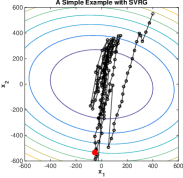
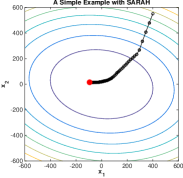
The most important property of the SVRG algorithm is the variance reduction of the steps. This property holds as the number of outer iteration grows, but it does not hold, if only the number of inner iterations increases. In other words, if we simply run the inner loop for many iterations (without executing additional outer loops), the variance of the steps does not reduce in the case of SVRG, while it goes to zero in the case of SARAH. To illustrate this effect, let us take a look at Figures 2 and 2.

In Figure 2, we applied one outer loop of SVRG and SARAH to a sum of 555 quadratic functions in a two-dimensional space, where the optimal solution is at the origin, the black lines and black dots indicate the trajectory of each algorithm and the red point indicates the final iterate. Initially, both SVRG and SARAH take steps along stochastic gradient directions towards the optimal solution. However, later iterations of SVRG wander randomly around the origin with large deviation from it, while SARAH follows a much more stable convergent trajectory, with a final iterate falling in a small neighborhood of the optimal solution.
Refer to caption
Refer to caption
Figure 1: A two-dimensional example of minwP(w)subscript𝑤𝑃𝑤\min_{w}P(w) with n=5𝑛5n=5 for SVRG (left) and SARAH (right).


Refer to caption      Refer to caption

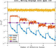
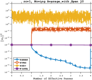
Figure 2: An example of 2subscript2\ell_{2}-regularized logistic regression on rcv1 training dataset for SARAH, SVRG, SGD+ and FISTA with multiple outer iterations (left) and a single outer iteration (right).

In Figure 2, the x-axis denotes the number of effective passes which is equivalent to the number of passes through all of the data in the dataset, the cost of each pass being equal to the cost of one full gradient evaluation; and y-axis represents vt2superscriptnormsubscript𝑣𝑡2\|v_{t}\|^{2}. Figure 2 shows the evolution of vt2superscriptnormsubscript𝑣𝑡2\|v_{t}\|^{2} for SARAH, SVRG, SGD+ (SGD with decreasing learning rate) and FISTA (an accelerated version of GD (Beck & Teboulle, 2009)) with m=4n𝑚4𝑛m=4n, where the left plot shows the trend over multiple outer iterations and the right plot shows a single outer iteration444In the plots of Figure 2, since the data for SVRG is noisy, we smooth it by using moving average filters with spans 100 for the left plot and 10 for the right one.. We can see that for SVRG, vt2superscriptnormsubscript𝑣𝑡2\|v_{t}\|^{2} decreases over the outer iterations, while it has an increasing trend or oscillating trend for each inner loop. In contrast, SARAH enjoys decreasing trends both in the outer and the inner loop iterations.

We will now show that the stochastic steps computed by SARAH converge linearly in the inner loop. We present two linear convergence results based on our two different assumptions of μ𝜇\mu-strong convexity. These results substantiate our conclusion that SARAH uses more stable stochastic gradient estimates than SVRG. The following theorem is our first result to demonstrate the linear convergence of our stochastic recursive step vtsubscript𝑣𝑡v_{t}.

Theorem 1a.

Suppose that Assumptions 1, 2a and 3 hold. Consider vtsubscript𝑣𝑡v_{t} defined by (2) in SARAH (Algorithm 1) with η<2/L𝜂2𝐿\eta<2/L. Then, for any t1𝑡1t\geq 1,

𝔼[vt2]𝔼delimited-[]superscriptnormsubscript𝑣𝑡2\displaystyle\mathbb{E}[\|v_{t}\|^{2}] [1(2ηL1)μ2η2]𝔼[vt12]absentdelimited-[]12𝜂𝐿1superscript𝜇2superscript𝜂2𝔼delimited-[]superscriptnormsubscript𝑣𝑡12\displaystyle\leq\left[1-\left(\tfrac{2}{\eta L}-1\right)\mu^{2}\eta^{2}\right]\mathbb{E}[\|v_{t-1}\|^{2}]
[1(2ηL1)μ2η2]t𝔼[P(w0)2].absentsuperscriptdelimited-[]12𝜂𝐿1superscript𝜇2superscript𝜂2𝑡𝔼delimited-[]superscriptnorm𝑃subscript𝑤02\displaystyle\leq\left[1-\left(\tfrac{2}{\eta L}-1\right)\mu^{2}\eta^{2}\right]^{t}\mathbb{E}[\|\nabla P(w_{0})\|^{2}].

This result implies that by choosing η=𝒪(1/L)𝜂𝒪1𝐿\eta=\operatorname{\mathcal{O}}(1/L), we obtain the linear convergence of vt2superscriptnormsubscript𝑣𝑡2\|v_{t}\|^{2} in expectation with the rate (11/κ2)11superscript𝜅2(1-1/\kappa^{2}). Below we show that a better convergence rate can be obtained under a stronger convexity assumption.

Theorem 1b.

Suppose that Assumptions 1 and 2b hold. Consider vtsubscript𝑣𝑡v_{t} defined by (2) in SARAH (Algorithm 1) with η2/(μ+L)𝜂2𝜇𝐿\eta\leq 2/(\mu+L). Then the following bound holds, t1for-all𝑡1\forall\ t\geq 1,

𝔼[vt2]𝔼delimited-[]superscriptnormsubscript𝑣𝑡2\displaystyle\mathbb{E}[\|v_{t}\|^{2}] (12μLημ+L)𝔼[vt12]absent12𝜇𝐿𝜂𝜇𝐿𝔼superscriptnormsubscript𝑣𝑡12\displaystyle\leq\left(1-\tfrac{2\mu L\eta}{\mu+L}\right)\operatorname{\mathbb{E}}[\|v_{t-1}\|^{2}]
(12μLημ+L)t𝔼[P(w0)2].absentsuperscript12𝜇𝐿𝜂𝜇𝐿𝑡𝔼superscriptnorm𝑃subscript𝑤02\displaystyle\leq\left(1-\tfrac{2\mu L\eta}{\mu+L}\right)^{t}\operatorname{\mathbb{E}}[\|\nabla P(w_{0})\|^{2}].

Again, by setting η=𝒪(1/L)𝜂𝒪1𝐿\eta=\operatorname{\mathcal{O}}(1/L), we derive the linear convergence with the rate of (11/κ)11𝜅(1-1/\kappa), which is a significant improvement over the result of Theorem 1a, when the problem is severely ill-conditioned.

3.2 Convergence Analysis

In this section, we derive the general convergence rate results for Algorithm 1. First, we present two important Lemmas as the foundation of our theory. Then, we proceed to prove sublinear convergence rate of a single outer iteration when applied to general convex functions. In the end, we prove that the algorithm with multiple outer iterations has linear convergence rate in the strongly convex case.

We begin with proving two useful lemmas that do not require any convexity assumption. The first Lemma 1 bounds the sum of expected values of P(wt)2superscriptnorm𝑃subscript𝑤𝑡2\|\nabla P(w_{t})\|^{2}. The second, Lemma 2, bounds 𝔼[P(wt)vt2]𝔼delimited-[]superscriptnorm𝑃subscript𝑤𝑡subscript𝑣𝑡2\mathbb{E}[\|\nabla P(w_{t})-v_{t}\|^{2}].

Lemma 1.

Suppose that Assumption 1 holds. Consider SARAH (Algorithm 1). Then, we have

t=0m𝔼[P(wt)2]2η𝔼[P(w0)P(w)]superscriptsubscript𝑡0𝑚𝔼delimited-[]superscriptnorm𝑃subscript𝑤𝑡22𝜂𝔼delimited-[]𝑃subscript𝑤0𝑃superscript𝑤\displaystyle\sum_{t=0}^{m}\mathbb{E}[\|\nabla P(w_{t})\|^{2}]\leq\frac{2}{\eta}\mathbb{E}[P(w_{0})-P(w^{*})] (8)
+t=0m𝔼[P(wt)vt2](1Lη)t=0m𝔼[vt2].superscriptsubscript𝑡0𝑚𝔼delimited-[]superscriptnorm𝑃subscript𝑤𝑡subscript𝑣𝑡21𝐿𝜂superscriptsubscript𝑡0𝑚𝔼delimited-[]superscriptnormsubscript𝑣𝑡2\displaystyle\quad+\sum_{t=0}^{m}\mathbb{E}[\|\nabla P(w_{t})-v_{t}\|^{2}]-(1-L\eta)\sum_{t=0}^{m}\mathbb{E}[\|v_{t}\|^{2}].
Lemma 2.

Suppose that Assumption 1 holds. Consider vtsubscript𝑣𝑡v_{t} defined by (2) in SARAH (Algorithm 1). Then for any t1𝑡1t\geq 1,

𝔼[P(wt)vt2]=j=1t𝔼[vjvj12]𝔼delimited-[]superscriptnorm𝑃subscript𝑤𝑡subscript𝑣𝑡2superscriptsubscript𝑗1𝑡𝔼delimited-[]superscriptnormsubscript𝑣𝑗subscript𝑣𝑗12\displaystyle\mathbb{E}[\|\nabla P(w_{t})-v_{t}\|^{2}]=\sum_{j=1}^{t}\mathbb{E}[\|v_{j}-v_{j-1}\|^{2}]
j=1t𝔼[P(wj)P(wj1)2].superscriptsubscript𝑗1𝑡𝔼delimited-[]superscriptnorm𝑃subscript𝑤𝑗𝑃subscript𝑤𝑗12\displaystyle\qquad\qquad-\sum_{j=1}^{t}\mathbb{E}[\|\nabla P(w_{j})-\nabla P(w_{j-1})\|^{2}].

Now we are ready to provide our main theoretical results.

3.2.1 General Convex Case

Following from Lemma 2, we can obtain the following upper bound for 𝔼[P(wt)vt2]𝔼delimited-[]superscriptnorm𝑃subscript𝑤𝑡subscript𝑣𝑡2\mathbb{E}[\|\nabla P(w_{t})-v_{t}\|^{2}] for convex functions fi,i[n]subscript𝑓𝑖𝑖delimited-[]𝑛f_{i},i\in[n].

Lemma 3.

Suppose that Assumptions 1 and 3 hold. Consider vtsubscript𝑣𝑡v_{t} defined as (2) in SARAH (Algorithm 1) with η<2/L𝜂2𝐿\eta<2/L. Then we have that for any t1𝑡1t\geq 1,

𝔼[P(wt)vt2]𝔼delimited-[]superscriptnorm𝑃subscript𝑤𝑡subscript𝑣𝑡2\displaystyle\mathbb{E}[\|\nabla P(w_{t})-v_{t}\|^{2}] ηL2ηL[𝔼[v02]𝔼[vt2]]absent𝜂𝐿2𝜂𝐿delimited-[]𝔼delimited-[]superscriptnormsubscript𝑣02𝔼delimited-[]superscriptnormsubscript𝑣𝑡2\displaystyle\leq\frac{\eta L}{2-\eta L}\Big{[}\mathbb{E}[\|v_{0}\|^{2}]-\mathbb{E}[\|v_{t}\|^{2}]\Big{]}
ηL2ηL𝔼[v02].absent𝜂𝐿2𝜂𝐿𝔼delimited-[]superscriptnormsubscript𝑣02\displaystyle\leq\frac{\eta L}{2-\eta L}\mathbb{E}[\|v_{0}\|^{2}]. (9)

Using the above lemmas, we can state and prove one of our core theorems as follows.

Theorem 2.

Suppose that Assumptions 1 and 3 hold. Consider SARAH (Algorithm 1) with η1/L𝜂1𝐿\eta\leq 1/L. Then for any s1𝑠1s\geq 1, we have

𝔼[P(w~s)2]𝔼delimited-[]superscriptnorm𝑃subscript~𝑤𝑠2\displaystyle\mathbb{E}[\|\nabla P(\tilde{w}_{s})\|^{2}] 2η(m+1)𝔼[P(w~s1)P(w)]absent2𝜂𝑚1𝔼delimited-[]𝑃subscript~𝑤𝑠1𝑃superscript𝑤\displaystyle\leq\frac{2}{\eta(m+1)}\mathbb{E}[P(\tilde{w}_{s-1})-P(w^{*})]
+ηL2ηL𝔼[P(w~s1)2].𝜂𝐿2𝜂𝐿𝔼delimited-[]superscriptnorm𝑃subscript~𝑤𝑠12\displaystyle\qquad+\frac{\eta L}{2-\eta L}\mathbb{E}[\|\nabla P(\tilde{w}_{s-1})\|^{2}]. (10)
Proof.

Since v0=P(w0)subscript𝑣0𝑃subscript𝑤0v_{0}=\nabla P(w_{0}) implies P(w0)v02=0superscriptnorm𝑃subscript𝑤0subscript𝑣020\|\nabla P(w_{0})-v_{0}\|^{2}=0 then by Lemma 3, we can write

t=0m𝔼[P(wt)vt2]mηL2ηL𝔼[v02].superscriptsubscript𝑡0𝑚𝔼delimited-[]superscriptnorm𝑃subscript𝑤𝑡subscript𝑣𝑡2𝑚𝜂𝐿2𝜂𝐿𝔼delimited-[]superscriptnormsubscript𝑣02\displaystyle\textstyle{\sum}_{t=0}^{m}\mathbb{E}[\|\nabla P(w_{t})-v_{t}\|^{2}]\leq\frac{m\eta L}{2-\eta L}\mathbb{E}[\|v_{0}\|^{2}]. (11)

Hence, by Lemma 1 with η1/L𝜂1𝐿\eta\leq 1/L, we have

t=0m𝔼[P(wt)2]superscriptsubscript𝑡0𝑚𝔼delimited-[]superscriptnorm𝑃subscript𝑤𝑡2\displaystyle\textstyle{\sum}_{t=0}^{m}\mathbb{E}[\|\nabla P(w_{t})\|^{2}]
2η𝔼[P(w0)P(w)]+t=0m𝔼[P(wt)vt2]absent2𝜂𝔼delimited-[]𝑃subscript𝑤0𝑃superscript𝑤superscriptsubscript𝑡0𝑚𝔼delimited-[]superscriptnorm𝑃subscript𝑤𝑡subscript𝑣𝑡2\displaystyle\leq\tfrac{2}{\eta}\mathbb{E}[P(w_{0})-P(w^{*})]+\textstyle{\sum}_{t=0}^{m}\mathbb{E}[\|\nabla P(w_{t})-v_{t}\|^{2}]
(11)2η𝔼[P(w0)P(w)]+mηL2ηL𝔼[v02].italic-(11italic-)2𝜂𝔼delimited-[]𝑃subscript𝑤0𝑃superscript𝑤𝑚𝜂𝐿2𝜂𝐿𝔼delimited-[]superscriptnormsubscript𝑣02\displaystyle\overset{\eqref{eq:abcdef}}{\leq}\tfrac{2}{\eta}\mathbb{E}[P(w_{0})-P(w^{*})]+\tfrac{m\eta L}{2-\eta L}\mathbb{E}[\|v_{0}\|^{2}]. (12)

Since we are considering one outer iteration, with s1𝑠1s\geq 1, then we have v0=P(w0)=P(w~s1)subscript𝑣0𝑃subscript𝑤0𝑃subscript~𝑤𝑠1v_{0}=\nabla P(w_{0})=\nabla P(\tilde{w}_{s-1}) (since w0=w~s1subscript𝑤0subscript~𝑤𝑠1w_{0}=\tilde{w}_{s-1}), and w~s=wtsubscript~𝑤𝑠subscript𝑤𝑡\tilde{w}_{s}=w_{t}, where t𝑡t is picked uniformly at random from {0,1,,m}01𝑚\{0,1,\dots,m\}. Therefore, the following holds,

𝔼[P(w~s)2]𝔼delimited-[]superscriptnorm𝑃subscript~𝑤𝑠2\displaystyle\mathbb{E}[\|\nabla P(\tilde{w}_{s})\|^{2}] =1m+1t=0m𝔼[P(wt)2]absent1𝑚1superscriptsubscript𝑡0𝑚𝔼delimited-[]superscriptnorm𝑃subscript𝑤𝑡2\displaystyle=\tfrac{1}{m+1}\textstyle{\sum}_{t=0}^{m}\mathbb{E}[\|\nabla P(w_{t})\|^{2}]
(12)2η(m+1)𝔼[P(w~s1)P(w)]italic-(12italic-)2𝜂𝑚1𝔼delimited-[]𝑃subscript~𝑤𝑠1𝑃superscript𝑤\displaystyle\overset{\eqref{eq:thm1conv}}{\leq}\tfrac{2}{\eta(m+1)}\mathbb{E}[P(\tilde{w}_{s-1})-P(w^{*})]
+ηL2ηL𝔼[P(w~s1)2].𝜂𝐿2𝜂𝐿𝔼delimited-[]superscriptnorm𝑃subscript~𝑤𝑠12\displaystyle\qquad+\tfrac{\eta L}{2-\eta L}\mathbb{E}[\|\nabla P(\tilde{w}_{s-1})\|^{2}].\qed

Theorem 2, in the case when η1/L𝜂1𝐿\eta\leq 1/L implies that

𝔼[P(w~s)2]𝔼delimited-[]superscriptnorm𝑃subscript~𝑤𝑠2\displaystyle\mathbb{E}[\|\nabla P(\tilde{w}_{s})\|^{2}] 2η(m+1)𝔼[P(w~s1)P(w)]absent2𝜂𝑚1𝔼delimited-[]𝑃subscript~𝑤𝑠1𝑃superscript𝑤\displaystyle\leq\tfrac{2}{\eta(m+1)}\mathbb{E}[P(\tilde{w}_{s-1})-P(w^{*})]
+ηL𝔼[P(w~s1)2].𝜂𝐿𝔼delimited-[]superscriptnorm𝑃subscript~𝑤𝑠12\displaystyle\qquad+{\eta L}\mathbb{E}[\|\nabla P(\tilde{w}_{s-1})\|^{2}].

By choosing the learning rate η=2L(m+1)𝜂2𝐿𝑚1\eta=\sqrt{\frac{2}{L(m+1)}} (with m𝑚m such that 2L(m+1)1/L2𝐿𝑚11𝐿\sqrt{\frac{2}{L(m+1)}}\leq 1/L) we can derive the following convergence result,

𝔼[P(w~s)2]𝔼delimited-[]superscriptnorm𝑃subscript~𝑤𝑠2\displaystyle\mathbb{E}[\|\nabla P(\tilde{w}_{s})\|^{2}]
2Lm+1𝔼[P(w~s1)P(w)+P(w~s1)2].absent2𝐿𝑚1𝔼delimited-[]𝑃subscript~𝑤𝑠1𝑃superscript𝑤superscriptnorm𝑃subscript~𝑤𝑠12\displaystyle\qquad\leq\sqrt{\tfrac{2L}{m+1}}\mathbb{E}[P(\tilde{w}_{s-1})-P(w^{*})+\|\nabla P(\tilde{w}_{s-1})\|^{2}].

Clearly, this result shows a sublinear convergence rate for SARAH under general convexity assumption within a single inner loop, with increasing m𝑚m, and consequently, we have the following result for complexity bound.

Corollary 1.

Suppose that Assumptions 1 and 3 hold. Consider SARAH (Algorithm 1) within a single outer iteration with the learning rate η=2L(m+1)𝜂2𝐿𝑚1\eta=\sqrt{\frac{2}{L(m+1)}} where m2L1𝑚2𝐿1m\geq 2L-1 is the total number of iterations, then P(wt)2superscriptnorm𝑃subscript𝑤𝑡2\|\nabla P(w_{t})\|^{2} converges sublinearly in expectation with a rate of 2Lm+12𝐿𝑚1\sqrt{\frac{2L}{m+1}}, and therefore, the total complexity to achieve an ϵitalic-ϵ\epsilon-accurate solution defined in (7) is 𝒪(n+1/ϵ2)𝒪𝑛1superscriptitalic-ϵ2\operatorname{\mathcal{O}}(n+1/\epsilon^{2}).

Refer to caption
Refer to caption
Refer to caption
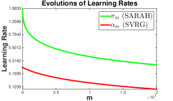
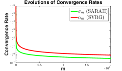
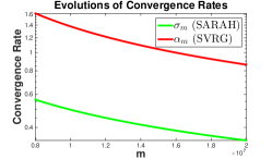
Figure 3: Theoretical comparisons of learning rates (left) and convergence rates (middle and right) with n=1,000,000𝑛1000000n=1,000,000 for SVRG and SARAH in one inner loop.

We now turn to estimating convergence of SARAH with multiple outer steps. Simply using Theorem 2 for each of the outer steps we have the following result.

Theorem 3.

Suppose that Assumptions 1 and 3 hold. Consider SARAH (Algorithm 1) and define

δksubscript𝛿𝑘\displaystyle\delta_{k} =2η(m+1)𝔼[P(w~k)P(w)],k=0,1,,s1,formulae-sequenceabsent2𝜂𝑚1𝔼delimited-[]𝑃subscript~𝑤𝑘𝑃superscript𝑤𝑘01𝑠1\displaystyle=\tfrac{2}{\eta(m+1)}\mathbb{E}[P(\tilde{w}_{k})-P(w^{*})],\ k=0,1,\dots,s-1,

and δ=max0ks1δk𝛿subscript0𝑘𝑠1subscript𝛿𝑘\delta=\max_{0\leq k\leq s-1}\delta_{k}. Then we have

𝔼[P(w~s)2]Δαs(P(w~0)2Δ),𝔼delimited-[]superscriptnorm𝑃subscript~𝑤𝑠2Δsuperscript𝛼𝑠superscriptnorm𝑃subscript~𝑤02Δ\displaystyle\mathbb{E}[\|\nabla P(\tilde{w}_{s})\|^{2}]-\Delta\leq\alpha^{s}(\|\nabla P(\tilde{w}_{0})\|^{2}-\Delta), (13)

where Δ=δ(1+ηL2(1ηL)),Δ𝛿1𝜂𝐿21𝜂𝐿\Delta=\delta\left(1+\tfrac{\eta L}{2(1-\eta L)}\right), and α=ηL2ηL.𝛼𝜂𝐿2𝜂𝐿\alpha=\tfrac{\eta L}{2-\eta L}.

Based on Theorem 3, we have the following total complexity for SARAH in the general convex case.

Corollary 2.

Let us choose Δ=ϵ/4Δitalic-ϵ4\Delta=\epsilon/4, α=1/2𝛼12\alpha=1/2 (with η=2/(3L)𝜂23𝐿\eta=2/(3L)), and m=𝒪(1/ϵ)𝑚𝒪1italic-ϵm=\operatorname{\mathcal{O}}(1/\epsilon) in Theorem 3. Then, the total complexity to achieve an ϵitalic-ϵ\epsilon-accuracy solution defined in (7) is 𝒪((n+(1/ϵ))log(1/ϵ))𝒪𝑛1italic-ϵ1italic-ϵ\operatorname{\mathcal{O}}((n+(1/\epsilon))\log(1/\epsilon)).

3.2.2 Strongly Convex Case

We now turn to the discussion of the linear convergence rate of SARAH under the strong convexity assumption on P𝑃P. From Theorem 2, for any s1𝑠1s\geq 1, using property (6) of the μ𝜇\mu-strongly convex P𝑃P, we have

𝔼[P(w~s)2]2η(m+1)𝔼[P(w~s1)P(w)]𝔼delimited-[]superscriptnorm𝑃subscript~𝑤𝑠22𝜂𝑚1𝔼delimited-[]𝑃subscript~𝑤𝑠1𝑃superscript𝑤\displaystyle\mathbb{E}[\|\nabla P(\tilde{w}_{s})\|^{2}]\leq\tfrac{2}{\eta(m+1)}\mathbb{E}[P(\tilde{w}_{s-1})-P(w^{*})]
+ηL2ηL𝔼[P(w~s1)2]𝜂𝐿2𝜂𝐿𝔼delimited-[]superscriptnorm𝑃subscript~𝑤𝑠12\displaystyle\qquad\qquad\qquad\qquad+\tfrac{\eta L}{2-\eta L}\mathbb{E}[\|\nabla P(\tilde{w}_{s-1})\|^{2}]
(6)(1μη(m+1)+ηL2ηL)𝔼[P(w~s1)2],italic-(6italic-)1𝜇𝜂𝑚1𝜂𝐿2𝜂𝐿𝔼delimited-[]superscriptnorm𝑃subscript~𝑤𝑠12\displaystyle\qquad\overset{\eqref{eq:strongconvexity2}}{\leq}\left(\tfrac{1}{\mu\eta(m+1)}+\tfrac{\eta L}{2-\eta L}\right)\mathbb{E}[\|\nabla P(\tilde{w}_{s-1})\|^{2}],

and equivalently,

𝔼[P(w~s)2]σm𝔼[P(w~s1)2].𝔼superscriptnorm𝑃subscript~𝑤𝑠2subscript𝜎𝑚𝔼superscriptnorm𝑃subscript~𝑤𝑠12\operatorname{\mathbb{E}}[\|\nabla P(\tilde{w}_{s})\|^{2}]\leq\sigma_{m}\operatorname{\mathbb{E}}[\|\nabla P(\tilde{w}_{s-1})\|^{2}]. (14)

Let us define σm=def1μη(m+1)+ηL2ηLsuperscriptdefsubscript𝜎𝑚1𝜇𝜂𝑚1𝜂𝐿2𝜂𝐿\sigma_{m}\stackrel{{\scriptstyle\text{def}}}{{=}}\tfrac{1}{\mu\eta(m+1)}+\tfrac{\eta L}{2-\eta L}. Then by choosing η𝜂\eta and m𝑚m such that σm<1subscript𝜎𝑚1\sigma_{m}<1, and applying (14) recursively, we are able to reach the following convergence result.

Theorem 4.

Suppose that Assumptions 1, 2a and 3 hold. Consider SARAH (Algorithm 1) with the choice of η𝜂\eta and m𝑚m such that

σm=def1μη(m+1)+ηL2ηL<1.superscriptdefsubscript𝜎𝑚1𝜇𝜂𝑚1𝜂𝐿2𝜂𝐿1\sigma_{m}\stackrel{{\scriptstyle\text{def}}}{{=}}\frac{1}{\mu\eta(m+1)}+\frac{\eta L}{2-\eta L}<1. (15)

Then, we have

𝔼[P(w~s)2](σm)sP(w~0)2.𝔼delimited-[]superscriptnorm𝑃subscript~𝑤𝑠2superscriptsubscript𝜎𝑚𝑠superscriptnorm𝑃subscript~𝑤02\displaystyle\mathbb{E}[\|\nabla P(\tilde{w}_{s})\|^{2}]\leq(\sigma_{m})^{s}\|\nabla P(\tilde{w}_{0})\|^{2}.
Remark 1.

Theorem 4 implies that any η<1/L𝜂1𝐿\eta<1/L will work for SARAH. Let us compare our convergence rate to that of SVRG. The linear rate of SVRG, as presented in (Johnson & Zhang, 2013), is given by

αm=1μη(12Lη)m+2ηL12ηL<1.subscript𝛼𝑚1𝜇𝜂12𝐿𝜂𝑚2𝜂𝐿12𝜂𝐿1\displaystyle\alpha_{m}=\tfrac{1}{\mu\eta(1-2L\eta)m}+\tfrac{2\eta L}{1-2\eta L}<1.

We observe that it implies that the learning rate has to satisfy η<1/(4L)𝜂14𝐿\eta<1/(4L), which is a tighter restriction than η<1/L𝜂1𝐿\eta<1/L required by SARAH. In addition, with the same values of m𝑚m and η𝜂\eta, the rate or convergence of (the outer iterations) of SARAH is always smaller than that of SVRG.

σmsubscript𝜎𝑚\displaystyle\sigma_{m} =1μη(m+1)+ηL2ηL=1μη(m+1)+12/(ηL)1absent1𝜇𝜂𝑚1𝜂𝐿2𝜂𝐿1𝜇𝜂𝑚112𝜂𝐿1\displaystyle=\tfrac{1}{\mu\eta(m+1)}+\tfrac{\eta L}{2-\eta L}=\tfrac{1}{\mu\eta(m+1)}+\tfrac{1}{2/(\eta L)-1}
<1μη(12Lη)m+10.5/(ηL)1=αm.absent1𝜇𝜂12𝐿𝜂𝑚10.5𝜂𝐿1subscript𝛼𝑚\displaystyle<\tfrac{1}{\mu\eta(1-2L\eta)m}+\tfrac{1}{0.5/(\eta L)-1}=\alpha_{m}.
Remark 2.

To further demonstrate the better convergence properties of SARAH, let us consider following optimization problem

min0<η<1/Lσm,min0<η<1/4Lαm,subscript0𝜂1𝐿subscript𝜎𝑚subscript0𝜂14𝐿subscript𝛼𝑚\min_{0<\eta<1/L}\ \sigma_{m},\qquad\min_{0<\eta<1/{4L}}\ \alpha_{m},

which can be interpreted as the best convergence rates for different values of m𝑚m, for both SARAH and SVRG. After simple calculations, we plot both learning rates and the corresponding theoretical rates of convergence, as shown in Figure 3, where the right plot is a zoom-in on a part of the middle plot. The left plot shows that the optimal learning rate for SARAH is significantly larger than that of SVRG, while the other two plots show significant improvement upon outer iteration convergence rates for SARAH over SVRG.

Based on Theorem 4, we are able to derive the following total complexity for SARAH in the strongly convex case.

Corollary 3.

Fix ϵ(0,1)italic-ϵ01\epsilon\in(0,1), and let us run SARAH with η=1/(2L)𝜂12𝐿\eta=1/(2L) and m=4.5κ𝑚4.5𝜅m=4.5\kappa for 𝒯𝒯\mathcal{T} iterations where 𝒯=log(P(w~0)2/ϵ)/log(9/7),𝒯superscriptnorm𝑃subscript~𝑤02italic-ϵ97\mathcal{T}=\lceil\log(\|\nabla P(\tilde{w}_{0})\|^{2}/\epsilon)/\log(9/7)\rceil, then we can derive an ϵitalic-ϵ\epsilon-accuracy solution defined in (7). Furthermore, we can obtain the total complexity of SARAH, to achieve the ϵitalic-ϵ\epsilon-accuracy solution, as 𝒪((n+κ)log(1/ϵ)).𝒪𝑛𝜅1italic-ϵ\operatorname{\mathcal{O}}\left((n+\kappa)\log(1/\epsilon)\right).

4 A Practical Variant

While SVRG is an efficient variance-reducing stochastic gradient method, one of its main drawbacks is the sensitivity of the practical performance with respect to the choice of m𝑚m. It is know that m𝑚m should be around 𝒪(κ)𝒪𝜅\operatorname{\mathcal{O}}(\kappa),555 In practice, when n𝑛n is large, P(w)𝑃𝑤P(w) is often considered as a regularized Empirical Loss Minimization problem with regularization parameter λ=1n𝜆1𝑛\lambda=\frac{1}{n}, then κ𝒪(n).similar-to𝜅𝒪𝑛\kappa\sim\operatorname{\mathcal{O}}(n). while it still remains unknown that what the exact best choice is. In this section, we propose a practical variant of SARAH as SARAH+ (Algorithm 2), which provides an automatic and adaptive choice of the inner loop size m𝑚m. Guided by the linear convergence of the steps in the inner loop, demonstrated in Figure 2, we introduce a stopping criterion based on the values of vt2superscriptnormsubscript𝑣𝑡2\|v_{t}\|^{2} while upper-bounding the total number of steps by a large enough m𝑚m for robustness. The other modification compared to SARAH (Algorithm 1) is the more practical choice w~s=wtsubscript~𝑤𝑠subscript𝑤𝑡\tilde{w}_{s}=w_{t}, where t𝑡t is the last index of the particular inner loop, instead of randomly selected intermediate index.

Algorithm 2 SARAH+
  Parameters: the learning rate η>0𝜂0\eta>0, 0<γ10𝛾10<\gamma\leq 1 and the maximum inner loop size m𝑚m.
  Initialize: w~0subscript~𝑤0\tilde{w}_{0}
  Iterate:
  for s=1,2,𝑠12s=1,2,\dots do
     w0=w~s1subscript𝑤0subscript~𝑤𝑠1w_{0}=\tilde{w}_{s-1}
     v0=1ni=1nfi(w0)subscript𝑣01𝑛superscriptsubscript𝑖1𝑛subscript𝑓𝑖subscript𝑤0v_{0}=\frac{1}{n}\sum_{i=1}^{n}\nabla f_{i}(w_{0})
     w1=w0ηv0subscript𝑤1subscript𝑤0𝜂subscript𝑣0w_{1}=w_{0}-\eta v_{0}
     t=1𝑡1t=1
     while vt12>γv02superscriptnormsubscript𝑣𝑡12𝛾superscriptnormsubscript𝑣02\|v_{t-1}\|^{2}>\gamma\|v_{0}\|^{2} and t<m𝑡𝑚t<m do
        Sample itsubscript𝑖𝑡i_{t} uniformly at random from [n]delimited-[]𝑛[n]
        vt=fit(wt)fit(wt1)+vt1subscript𝑣𝑡subscript𝑓subscript𝑖𝑡subscript𝑤𝑡subscript𝑓subscript𝑖𝑡subscript𝑤𝑡1subscript𝑣𝑡1v_{t}=\nabla f_{i_{t}}(w_{t})-\nabla f_{i_{t}}(w_{t-1})+v_{t-1}
        wt+1=wtηvtsubscript𝑤𝑡1subscript𝑤𝑡𝜂subscript𝑣𝑡w_{t+1}=w_{t}-\eta v_{t}
        t=t+1𝑡𝑡1t=t+1
     end while
     Set w~s=wtsubscript~𝑤𝑠subscript𝑤𝑡\tilde{w}_{s}=w_{t}
  end for

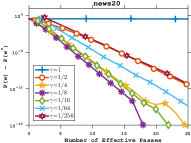
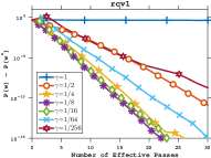
Different from SARAH, SARAH+ provides a possibility of earlier termination and unnecessary careful choices of m𝑚m, and it also covers the classical gradient descent when we set γ=1𝛾1\gamma=1 (since the while loop does not proceed). In Figure 4 we present the numerical performance of SARAH+ with different γ𝛾\gammas on rcv1 and news20 datasets. The size of the inner loop provides a trade-off between the fast sub-linear convergence in the inner loop and linear convergence in the outer loop. From the results, it appears that γ=1/8𝛾18\gamma=1/8 is the optimal choice. With a larger γ𝛾\gamma, i.e. γ>1/8𝛾18\gamma>1/8, the iterates in the inner loop do not provide sufficient reduction, before another full gradient computation is required, while with γ<1/8𝛾18\gamma<1/8 an unnecessary number of inner steps is performed without gaining substantial progress. Clearly γ𝛾\gamma is another parameter that requires tuning, however, in our experiments, the performance of SARAH+ has been very robust with respect to the choices of γ𝛾\gamma and did not vary much from one data set to another.

Similarly to SVRG, vt2superscriptnormsubscript𝑣𝑡2\|v_{t}\|^{2} decreases in the outer iterations of SARAH+. However, unlike SVRG, SARAH+ also inherits from SARAH the consistent decrease of vt2superscriptnormsubscript𝑣𝑡2\|v_{t}\|^{2} in expectation in the inner loops. It is not possible to apply the same idea of adaptively terminating the inner loop of SVRG based on the reduction in vt2superscriptnormsubscript𝑣𝑡2\|v_{t}\|^{2}, as vt2superscriptnormsubscript𝑣𝑡2\|v_{t}\|^{2} may have side fluctuations as shown in Figure 2.
Refer to caption
Refer to caption
Figure 4: An example of 2subscript2\ell_{2}-regularized logistic regression on rcv1 (left) and news20 (right) training datasets for SARAH+ with different γ𝛾\gammas on loss residuals P(w)P(w)𝑃𝑤𝑃superscript𝑤P(w)-P(w^{*}).

5 Numerical Experiments

Refer to caption
Refer to caption
Refer to caption
Refer to caption
Refer to caption
Refer to caption
Refer to caption
Refer to caption
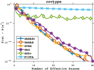
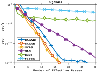
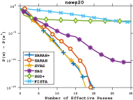
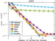
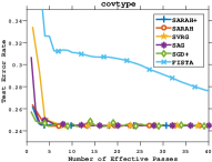
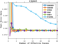
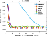
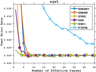
Figure 5: Comparisons of loss residuals P(w)P(w)𝑃𝑤𝑃superscript𝑤P(w)-P(w^{*}) (top) and test errors (bottom) from different modern stochastic methods on covtype, ijcnn1, news20 and rcv1.

To support the theoretical analyses and insights, we present our empirical experiments, comparing SARAH and SARAH+ with the state-of-the-art first-order methods for 2subscript2\ell_{2}-regularized logistic regression problems with

fi(w)=log(1+exp(yixiTw))+λ2w2,subscript𝑓𝑖𝑤1subscript𝑦𝑖superscriptsubscript𝑥𝑖𝑇𝑤𝜆2superscriptnorm𝑤2f_{i}(w)=\log(1+\exp(-y_{i}x_{i}^{T}w))+\tfrac{\lambda}{2}\|w\|^{2},

on datasets covtype, ijcnn1, news20 and rcv1 666All datasets are available at http://www.csie.ntu.edu.tw/~cjlin/libsvmtools/datasets/.. For ijcnn1 and rcv1 we use the predefined testing and training sets, while covtype and news20 do not have test data, hence we randomly split the datasets with 70%percent7070\% for training and 30%percent3030\% for testing. Some statistics of the datasets are summarized in Table 3.

Table 3: Summary of datasets used for experiments.
Dataset d𝑑d n𝑛n (train) Sparsity n𝑛n (test) L𝐿L
covtype 54 406,709 22.12% 174,303 1.90396
ijcnn1 22 91, 701 59.09% 49, 990 1.77662
news20 1,355,191 13, 997 0.03375% 5, 999 0.2500
rcv1 47,236 677,399 0.1549% 20,242 0.2500

The penalty parameter λ𝜆\lambda is set to 1/n1𝑛1/n as is common practice (Le Roux et al., 2012). Note that like SVRG/S2GD and SAG/SAGA, SARAH also allows an efficient sparse implementation named “lazy updates” (Konečný et al., 2016). We conduct and compare numerical results of SARAH with SVRG, SAG, SGD+ and FISTA. SVRG (Johnson & Zhang, 2013) and SAG (Le Roux et al., 2012) are classic modern stochastic methods. SGD+ is SGD with decreasing learning rate η=η0/(k+1)𝜂subscript𝜂0𝑘1\eta=\eta_{0}/(k+1) where k𝑘k is the number of effective passes and η0subscript𝜂0\eta_{0} is some initial constant learning rate. FISTA (Beck & Teboulle, 2009) is the Fast Iterative Shrinkage-Thresholding Algorithm, well-known as an efficient accelerated version of the gradient descent. Even though for each method, there is a theoretical safe learning rate, we compare the results for the best learning rates in hindsight.

Figure 5 shows numerical results in terms of loss residuals (top) and test errors (bottom) on the four datasets, SARAH is sometimes comparable or a little worse than other methods at the beginning. However, it quickly catches up to or surpasses all other methods, demonstrating a faster rate of decrease across all experiments. We observe that on covtype and rcv1, SARAH, SVRG and SAG are comparable with some advantage of SARAH on covtype. On ijcnn1 and news20, SARAH and SVRG consistently surpass the other methods.

Table 4: Summary of best parameters for all the algorithms on different datasets.
Dataset SARAH (m,η)superscript𝑚superscript𝜂(m^{*},\eta^{*}) SVRG (m,η)superscript𝑚superscript𝜂(m^{*},\eta^{*}) SAG (ηsuperscript𝜂\eta^{*}) SGD+ (ηsuperscript𝜂\eta^{*}) FISTA (ηsuperscript𝜂\eta^{*})
covtype (2n, 0.9/L) (n, 0.8/L) 0.3/L 0.06/L 50/L
ijcnn1 (0.5n, 0.8/L) (n, 0.5/L) 0.7/L 0.1/L 90/L
news20 (0.5n, 0.9/L) (n, 0.5/L) 0.1/L 0.2/L 30/L
rcv1 (0.7n, 0.7/L) (0.5n, 0.9/L) 0.1/L 0.1/L 120/L

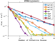
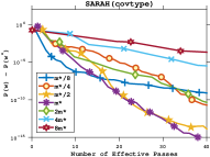
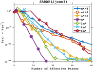
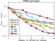
In particular, to validate the efficiency of our practical variant SARAH+, we provide an insight into how important the choices of m𝑚m and η𝜂\eta are for SVRG and SARAH in Table 4 and Figure 6. Table 4 presents the optimal choices of m𝑚m and η𝜂\eta for each of the algorithm, while Figure 6 shows the behaviors of SVRG and SARAH with different choices of m𝑚m for covtype and ijcnn1, where msuperscript𝑚m^{*}s denote the best choices. In Table 4, the optimal learning rates of SARAH vary less among different datasets compared to all the other methods and they approximate the theoretical upper bound for SARAH (1/L1𝐿1/L); on the contrary, for the other methods the empirical optimal rates can exceed their theoretical limits (SVRG with 1/(4L)14𝐿1/(4L), SAG with 1/(16L)116𝐿1/(16L), FISTA with 1/L1𝐿1/L). This empirical studies suggest that it is much easier to tune and find the ideal learning rate for SARAH. As observed in Figure 6, the behaviors of both SARAH and SVRG are quite sensitive to the choices of m𝑚m. With improper choices of m𝑚m, the loss residuals can be increased considerably from 1015superscript101510^{-15} to 103superscript10310^{-3} on both covtype in 40 effective passes and ijcnn1 in 17 effective passes for SARAH/SVRG.
Refer to caption
Refer to caption
Refer to caption
Refer to caption
Figure 6: Comparisons of loss residuals P(w)P(w)𝑃𝑤𝑃superscript𝑤P(w)-P(w^{*}) for different inner loop sizes with SVRG (top) and SARAH (bottom) on covtype and ijcnn1.

6 Conclusion

We propose a new variance reducing stochastic recursive gradient algorithm SARAH, which combines some of the properties of well known existing algorithms, such as SAGA and SVRG. For smooth convex functions, we show a sublinear convergence rate, while for strongly convex cases, we prove the linear convergence rate and the computational complexity as those of SVRG and SAG. However, compared to SVRG, SARAH’s convergence rate constant is smaller and the algorithms is more stable both theoretically and numerically. Additionally, we prove the linear convergence for inner loops of SARAH which support the claim of stability. Based on this convergence we derive a practical version of SARAH, with a simple stopping criterion for the inner loops.

Acknowledgements

The authors would like to thank the reviewers for useful suggestions which helped to improve the exposition in the paper.

References

  • Allen-Zhu (2017) Allen-Zhu, Zeyuan. Katyusha: The First Direct Acceleration of Stochastic Gradient Methods. Proceedings of the 49th Annual ACM on Symposium on Theory of Computing (to appear), 2017.
  • Allen-Zhu & Yuan (2016) Allen-Zhu, Zeyuan and Yuan, Yang. Improved SVRG for Non-Strongly-Convex or Sum-of-Non-Convex Objectives. In ICML, pp.  1080–1089, 2016.
  • Beck & Teboulle (2009) Beck, Amir and Teboulle, Marc. A fast iterative shrinkage-thresholding algorithm for linear inverse problems. SIAM J. Imaging Sciences, 2(1):183–202, 2009.
  • Bottou (1998) Bottou, Léon. Online learning and stochastic approximations. In Saad, David (ed.), Online Learning in Neural Networks, pp. 9–42. Cambridge University Press, New York, NY, USA, 1998. ISBN 0-521-65263-4.
  • Bottou et al. (2016) Bottou, Léon, Curtis, Frank E, and Nocedal, Jorge. Optimization methods for large-scale machine learning. arXiv:1606.04838, 2016.
  • Cotter et al. (2011) Cotter, Andrew, Shamir, Ohad, Srebro, Nati, and Sridharan, Karthik. Better mini-batch algorithms via accelerated gradient methods. In NIPS, pp.  1647–1655, 2011.
  • Defazio et al. (2014) Defazio, Aaron, Bach, Francis, and Lacoste-Julien, Simon. SAGA: A fast incremental gradient method with support for non-strongly convex composite objectives. In NIPS, pp.  1646–1654, 2014.
  • Hastie et al. (2009) Hastie, Trevor, Tibshirani, Robert, and Friedman, Jerome. The Elements of Statistical Learning: Data Mining, Inference, and Prediction. Springer Series in Statistics, 2nd edition, 2009.
  • Johnson & Zhang (2013) Johnson, Rie and Zhang, Tong. Accelerating stochastic gradient descent using predictive variance reduction. In NIPS, pp.  315–323, 2013.
  • Konečný et al. (2016) Konečný, Jakub, Liu, Jie, Richtárik, Peter, and Takáč, Martin. Mini-batch semi-stochastic gradient descent in the proximal setting. IEEE Journal of Selected Topics in Signal Processing, 10:242–255, 2016.
  • Konečný & Richtárik (2013) Konečný, Jakub and Richtárik, Peter. Semi-stochastic gradient descent methods. arXiv:1312.1666, 2013.
  • Le Roux et al. (2012) Le Roux, Nicolas, Schmidt, Mark, and Bach, Francis. A stochastic gradient method with an exponential convergence rate for finite training sets. In NIPS, pp.  2663–2671, 2012.
  • Mairal (2013) Mairal, Julien. Optimization with first-order surrogate functions. In ICML, pp.  783–791, 2013.
  • Mokhtari et al. (2017) Mokhtari, Aryan, Gürbüzbalaban, Mert, and Ribeiro, Alejandro. A double incremental aggregated gradient method with linear convergence rate for large-scale optimization. Proceedings of IEEE International Conference on Acoustic, Speech and Signal Processing (to appear), 2017.
  • Nesterov (2004) Nesterov, Yurii. Introductory lectures on convex optimization : a basic course. Applied optimization. Kluwer Academic Publ., Boston, Dordrecht, London, 2004. ISBN 1-4020-7553-7.
  • Reddi et al. (2016) Reddi, Sashank J., Hefny, Ahmed, Sra, Suvrit, Póczos, Barnabás, and Smola, Alexander J. Stochastic variance reduction for nonconvex optimization. In ICML, pp.  314–323, 2016.
  • Robbins & Monro (1951) Robbins, Herbert and Monro, Sutton. A stochastic approximation method. The Annals of Mathematical Statistics, 22(3):400–407, 1951.
  • Schmidt et al. (2016) Schmidt, Mark, Le Roux, Nicolas, and Bach, Francis. Minimizing finite sums with the stochastic average gradient. Mathematical Programming, pp.  1–30, 2016.
  • Shalev-Shwartz & Zhang (2013) Shalev-Shwartz, Shai and Zhang, Tong. Stochastic dual coordinate ascent methods for regularized loss. Journal of Machine Learning Research, 14(1):567–599, 2013.
  • Shalev-Shwartz et al. (2007) Shalev-Shwartz, Shai, Singer, Yoram, and Srebro, Nathan. Pegasos: Primal estimated sub-gradient solver for SVM. In ICML, pp.  807–814, 2007.
  • Shalev-Shwartz et al. (2011) Shalev-Shwartz, Shai, Singer, Yoram, Srebro, Nathan, and Cotter, Andrew. Pegasos: Primal estimated sub-gradient solver for SVM. Mathematical Programming, 127(1):3–30, 2011.
  • Takáč et al. (2013) Takáč, Martin, Bijral, Avleen Singh, Richtárik, Peter, and Srebro, Nathan. Mini-batch primal and dual methods for SVMs. In ICML, pp.  1022–1030, 2013.
  • Xiao & Zhang (2014) Xiao, Lin and Zhang, Tong. A proximal stochastic gradient method with progressive variance reduction. SIAM Journal on Optimization, 24(4):2057–2075, 2014.

Appendix A Technical Results

Lemma 4 (Theorem 2.1.5 in (Nesterov, 2004)).

Suppose that f𝑓f is convex and L𝐿L-smooth. Then, for any w𝑤w, wdsuperscript𝑤superscript𝑑w^{\prime}\in\mathbb{R}^{d},

f(w)f(w)+f(w)T(ww)+L2ww2,𝑓𝑤𝑓superscript𝑤𝑓superscriptsuperscript𝑤𝑇𝑤superscript𝑤𝐿2superscriptnorm𝑤superscript𝑤2\displaystyle f(w)\leq f(w^{\prime})+\nabla f(w^{\prime})^{T}(w-w^{\prime})+\frac{L}{2}\|w-w^{\prime}\|^{2}, (16)
f(w)f(w)+f(w)T(ww)+12Lf(w)f(w)2,𝑓𝑤𝑓superscript𝑤𝑓superscriptsuperscript𝑤𝑇𝑤superscript𝑤12𝐿superscriptnorm𝑓𝑤𝑓superscript𝑤2\displaystyle f(w)\geq f(w^{\prime})+\nabla f(w^{\prime})^{T}(w-w^{\prime})+\frac{1}{2L}\|\nabla f(w)-\nabla f(w^{\prime})\|^{2}, (17)
(f(w)f(w))T(ww)1Lf(w)f(w)2.superscript𝑓𝑤𝑓superscript𝑤𝑇𝑤superscript𝑤1𝐿superscriptnorm𝑓𝑤𝑓superscript𝑤2\displaystyle(\nabla f(w)-\nabla f(w^{\prime}))^{T}(w-w^{\prime})\geq\frac{1}{L}\|\nabla f(w)-\nabla f(w^{\prime})\|^{2}. (18)

Note that (16) does not require the convexity of f𝑓f.

Lemma 5 (Theorem 2.1.11 in (Nesterov, 2004)).

Suppose that f𝑓f is μ𝜇\mu-strongly convex and L𝐿L-smooth. Then, for any w𝑤w, wdsuperscript𝑤superscript𝑑w^{\prime}\in\mathbb{R}^{d},

(f(w)f(w))T(ww)μLμ+Lww2+1μ+Lf(w)f(w)2.superscript𝑓𝑤𝑓superscript𝑤𝑇𝑤superscript𝑤𝜇𝐿𝜇𝐿superscriptnorm𝑤superscript𝑤21𝜇𝐿superscriptnorm𝑓𝑤𝑓superscript𝑤2\displaystyle(\nabla f(w)-\nabla f(w^{\prime}))^{T}(w-w^{\prime})\geq\frac{\mu L}{\mu+L}\|w-w^{\prime}\|^{2}+\frac{1}{\mu+L}\|\nabla f(w)-\nabla f(w^{\prime})\|^{2}. (19)
Lemma 6 (Choices of m𝑚m and η𝜂\eta).

Consider the rate of convergence σmsubscript𝜎𝑚\sigma_{m} in Theorem 4. If we choose η=1/(θL)𝜂1𝜃𝐿\eta=1/(\theta L) with θ>1𝜃1\theta>1 and fix σmsubscript𝜎𝑚\sigma_{m}, then the best choice of m𝑚m is

m=12(2θ1)2κ1,superscript𝑚12superscript2superscript𝜃12𝜅1m^{*}=\frac{1}{2}(2\theta^{*}-1)^{2}\kappa-1,

where κ=defL/μ,superscriptdef𝜅𝐿𝜇\kappa\stackrel{{\scriptstyle\text{def}}}{{=}}L/\mu, with θsuperscript𝜃\theta^{*} calculated as:

θ=σm+1+σm+12σm.superscript𝜃subscript𝜎𝑚1subscript𝜎𝑚12subscript𝜎𝑚\theta^{*}=\frac{\sigma_{m}+1+\sqrt{\sigma_{m}+1}}{2\sigma_{m}}.

Furthermore, we require θ>1+2/2superscript𝜃122\theta^{*}>1+\sqrt{2}/2 for σm<1subscript𝜎𝑚1\sigma_{m}<1.

Appendix B Proofs

B.1 Proof of Lemma 1

By Assumption 1 and wt+1=wtηvtsubscript𝑤𝑡1subscript𝑤𝑡𝜂subscript𝑣𝑡w_{t+1}=w_{t}-\eta v_{t}, we have

𝔼[P(wt+1)]𝔼delimited-[]𝑃subscript𝑤𝑡1\displaystyle\mathbb{E}[P(w_{t+1})] (16)𝔼[P(wt)]η𝔼[P(wt)Tvt]+Lη22𝔼[vt2]italic-(16italic-)𝔼delimited-[]𝑃subscript𝑤𝑡𝜂𝔼delimited-[]𝑃superscriptsubscript𝑤𝑡𝑇subscript𝑣𝑡𝐿superscript𝜂22𝔼delimited-[]superscriptnormsubscript𝑣𝑡2\displaystyle\overset{\eqref{eq:Lsmooth}}{\leq}\mathbb{E}[P(w_{t})]-\eta\mathbb{E}[\nabla P(w_{t})^{T}v_{t}]+\frac{L\eta^{2}}{2}\mathbb{E}[\|v_{t}\|^{2}]
=𝔼[P(wt)]η2𝔼[P(wt)2]+η2𝔼[P(wt)vt2](η2Lη22)𝔼[vt2],absent𝔼delimited-[]𝑃subscript𝑤𝑡𝜂2𝔼delimited-[]superscriptnorm𝑃subscript𝑤𝑡2𝜂2𝔼delimited-[]superscriptnorm𝑃subscript𝑤𝑡subscript𝑣𝑡2𝜂2𝐿superscript𝜂22𝔼delimited-[]superscriptnormsubscript𝑣𝑡2\displaystyle=\mathbb{E}[P(w_{t})]-\frac{\eta}{2}\mathbb{E}[\|\nabla P(w_{t})\|^{2}]+\frac{\eta}{2}\mathbb{E}[\|\nabla P(w_{t})-v_{t}\|^{2}]-\left(\frac{\eta}{2}-\frac{L\eta^{2}}{2}\right)\mathbb{E}[\|v_{t}\|^{2}],

where the last equality follows from the fact aTb=12[a2+b2ab2].superscript𝑎𝑇𝑏12delimited-[]superscriptnorm𝑎2superscriptnorm𝑏2superscriptnorm𝑎𝑏2a^{T}b=\frac{1}{2}\left[\|a\|^{2}+\|b\|^{2}-\|a-b\|^{2}\right].

By summing over t=0,,m𝑡0𝑚t=0,\dots,m, we have

𝔼[P(wm+1)]𝔼delimited-[]𝑃subscript𝑤𝑚1\displaystyle\mathbb{E}[P(w_{m+1})] 𝔼[P(w0)]η2t=0m𝔼[P(wt)2]+η2t=0m𝔼[P(wt)vt2](η2Lη22)t=0m𝔼[vt2],absent𝔼delimited-[]𝑃subscript𝑤0𝜂2superscriptsubscript𝑡0𝑚𝔼delimited-[]superscriptnorm𝑃subscript𝑤𝑡2𝜂2superscriptsubscript𝑡0𝑚𝔼delimited-[]superscriptnorm𝑃subscript𝑤𝑡subscript𝑣𝑡2𝜂2𝐿superscript𝜂22superscriptsubscript𝑡0𝑚𝔼delimited-[]superscriptnormsubscript𝑣𝑡2\displaystyle\leq\mathbb{E}[P(w_{0})]-\frac{\eta}{2}\sum_{t=0}^{m}\mathbb{E}[\|\nabla P(w_{t})\|^{2}]+\frac{\eta}{2}\sum_{t=0}^{m}\mathbb{E}[\|\nabla P(w_{t})-v_{t}\|^{2}]-\left(\frac{\eta}{2}-\frac{L\eta^{2}}{2}\right)\sum_{t=0}^{m}\mathbb{E}[\|v_{t}\|^{2}],

which is equivalent to (η>0𝜂0\eta>0):

t=0m𝔼[P(wt)2]superscriptsubscript𝑡0𝑚𝔼delimited-[]superscriptnorm𝑃subscript𝑤𝑡2\displaystyle\sum_{t=0}^{m}\mathbb{E}[\|\nabla P(w_{t})\|^{2}] 2η𝔼[P(w0)P(wm+1)]+t=0m𝔼[P(wt)vt2](1Lη)t=0m𝔼[vt2]absent2𝜂𝔼delimited-[]𝑃subscript𝑤0𝑃subscript𝑤𝑚1superscriptsubscript𝑡0𝑚𝔼delimited-[]superscriptnorm𝑃subscript𝑤𝑡subscript𝑣𝑡21𝐿𝜂superscriptsubscript𝑡0𝑚𝔼delimited-[]superscriptnormsubscript𝑣𝑡2\displaystyle\leq\frac{2}{\eta}\mathbb{E}[P(w_{0})-P(w_{m+1})]+\sum_{t=0}^{m}\mathbb{E}[\|\nabla P(w_{t})-v_{t}\|^{2}]-(1-L\eta)\sum_{t=0}^{m}\mathbb{E}[\|v_{t}\|^{2}]
2η𝔼[P(w0)P(w)]+t=0m𝔼[P(wt)vt2](1Lη)t=0m𝔼[vt2],absent2𝜂𝔼delimited-[]𝑃subscript𝑤0𝑃superscript𝑤superscriptsubscript𝑡0𝑚𝔼delimited-[]superscriptnorm𝑃subscript𝑤𝑡subscript𝑣𝑡21𝐿𝜂superscriptsubscript𝑡0𝑚𝔼delimited-[]superscriptnormsubscript𝑣𝑡2\displaystyle\leq\frac{2}{\eta}\mathbb{E}[P(w_{0})-P(w^{*})]+\sum_{t=0}^{m}\mathbb{E}[\|\nabla P(w_{t})-v_{t}\|^{2}]-(1-L\eta)\sum_{t=0}^{m}\mathbb{E}[\|v_{t}\|^{2}],

where the last inequality follows since wsuperscript𝑤w^{*} is a global minimizer of P𝑃P.

B.2 Proof of Lemma 2

Note that jsubscript𝑗\mathcal{F}_{j} contains all the information of w0,,wjsubscript𝑤0subscript𝑤𝑗w_{0},\dots,w_{j} as well as v0,,vj1subscript𝑣0subscript𝑣𝑗1v_{0},\dots,v_{j-1}. For j1𝑗1j\geq 1, we have

𝔼[P(wj)vj2|j]𝔼delimited-[]conditionalsuperscriptnorm𝑃subscript𝑤𝑗subscript𝑣𝑗2subscript𝑗\displaystyle\mathbb{E}[\|\nabla P(w_{j})-v_{j}\|^{2}|\mathcal{F}_{j}] =𝔼[[P(wj1)vj1]+[P(wj)P(wj1)][vjvj1]2|j]absent𝔼delimited-[]conditionalsuperscriptnormdelimited-[]𝑃subscript𝑤𝑗1subscript𝑣𝑗1delimited-[]𝑃subscript𝑤𝑗𝑃subscript𝑤𝑗1delimited-[]subscript𝑣𝑗subscript𝑣𝑗12subscript𝑗\displaystyle=\mathbb{E}[\|[\nabla P(w_{j-1})-v_{j-1}]+[\nabla P(w_{j})-\nabla P(w_{j-1})]-[v_{j}-v_{j-1}]\|^{2}|\mathcal{F}_{j}]
=P(wj1)vj12+P(wj)P(wj1)2+𝔼[vjvj12|j]absentsuperscriptnorm𝑃subscript𝑤𝑗1subscript𝑣𝑗12superscriptnorm𝑃subscript𝑤𝑗𝑃subscript𝑤𝑗12𝔼delimited-[]conditionalsuperscriptnormsubscript𝑣𝑗subscript𝑣𝑗12subscript𝑗\displaystyle=\|\nabla P(w_{j-1})-v_{j-1}\|^{2}+\|\nabla P(w_{j})-\nabla P(w_{j-1})\|^{2}+\mathbb{E}[\|v_{j}-v_{j-1}\|^{2}|\mathcal{F}_{j}]
+2(P(wj1)vj1)T(P(wj)P(wj1))2superscript𝑃subscript𝑤𝑗1subscript𝑣𝑗1𝑇𝑃subscript𝑤𝑗𝑃subscript𝑤𝑗1\displaystyle\quad+2(\nabla P(w_{j-1})-v_{j-1})^{T}(\nabla P(w_{j})-\nabla P(w_{j-1}))
2(P(wj1)vj1)T𝔼[vjvj1|j]2superscript𝑃subscript𝑤𝑗1subscript𝑣𝑗1𝑇𝔼delimited-[]subscript𝑣𝑗conditionalsubscript𝑣𝑗1subscript𝑗\displaystyle\quad-2(\nabla P(w_{j-1})-v_{j-1})^{T}\mathbb{E}[v_{j}-v_{j-1}|\mathcal{F}_{j}]
2(P(wj)P(wj1))T𝔼[vjvj1|j]2superscript𝑃subscript𝑤𝑗𝑃subscript𝑤𝑗1𝑇𝔼delimited-[]subscript𝑣𝑗conditionalsubscript𝑣𝑗1subscript𝑗\displaystyle\quad-2(\nabla P(w_{j})-\nabla P(w_{j-1}))^{T}\mathbb{E}[v_{j}-v_{j-1}|\mathcal{F}_{j}]
=P(wj1)vj12P(wj)P(wj1)2+𝔼[vjvj12|j],absentsuperscriptnorm𝑃subscript𝑤𝑗1subscript𝑣𝑗12superscriptnorm𝑃subscript𝑤𝑗𝑃subscript𝑤𝑗12𝔼delimited-[]conditionalsuperscriptnormsubscript𝑣𝑗subscript𝑣𝑗12subscript𝑗\displaystyle=\|\nabla P(w_{j-1})-v_{j-1}\|^{2}-\|\nabla P(w_{j})-\nabla P(w_{j-1})\|^{2}+\mathbb{E}[\|v_{j}-v_{j-1}\|^{2}|\mathcal{F}_{j}],

where the last equality follows from

𝔼[vjvj1|j]=(2)𝔼[fij(wj)fij(wj1)|j]=P(wj)P(wj1).𝔼delimited-[]subscript𝑣𝑗conditionalsubscript𝑣𝑗1subscript𝑗italic-(2italic-)𝔼delimited-[]subscript𝑓subscript𝑖𝑗subscript𝑤𝑗conditionalsubscript𝑓subscript𝑖𝑗subscript𝑤𝑗1subscript𝑗𝑃subscript𝑤𝑗𝑃subscript𝑤𝑗1\displaystyle\mathbb{E}[v_{j}-v_{j-1}|\mathcal{F}_{j}]\overset{\eqref{eq:vt}}{=}\mathbb{E}[\nabla f_{i_{j}}(w_{j})-\nabla f_{i_{j}}(w_{j-1})|\mathcal{F}_{j}]=\nabla P(w_{j})-\nabla P(w_{j-1}).

By taking expectation for the above equation, we have

𝔼[P(wj)vj2]𝔼delimited-[]superscriptnorm𝑃subscript𝑤𝑗subscript𝑣𝑗2\displaystyle\mathbb{E}[\|\nabla P(w_{j})-v_{j}\|^{2}] =𝔼[P(wj1)vj12]𝔼[P(wj)P(wj1)2]+𝔼[vjvj12].absent𝔼delimited-[]superscriptnorm𝑃subscript𝑤𝑗1subscript𝑣𝑗12𝔼delimited-[]superscriptnorm𝑃subscript𝑤𝑗𝑃subscript𝑤𝑗12𝔼delimited-[]superscriptnormsubscript𝑣𝑗subscript𝑣𝑗12\displaystyle=\mathbb{E}[\|\nabla P(w_{j-1})-v_{j-1}\|^{2}]-\mathbb{E}[\|\nabla P(w_{j})-\nabla P(w_{j-1})\|^{2}]+\mathbb{E}[\|v_{j}-v_{j-1}\|^{2}].

Note that P(w0)v02=0superscriptnorm𝑃subscript𝑤0subscript𝑣020\|\nabla P(w_{0})-v_{0}\|^{2}=0. By summing over j=1,,t(t1)𝑗1𝑡𝑡1j=1,\dots,t\ (t\geq 1), we have

𝔼[P(wt)vt2]=j=1t𝔼[vjvj12]j=1t𝔼[P(wj)P(wj1)2].𝔼delimited-[]superscriptnorm𝑃subscript𝑤𝑡subscript𝑣𝑡2superscriptsubscript𝑗1𝑡𝔼delimited-[]superscriptnormsubscript𝑣𝑗subscript𝑣𝑗12superscriptsubscript𝑗1𝑡𝔼delimited-[]superscriptnorm𝑃subscript𝑤𝑗𝑃subscript𝑤𝑗12\displaystyle\mathbb{E}[\|\nabla P(w_{t})-v_{t}\|^{2}]=\sum_{j=1}^{t}\mathbb{E}[\|v_{j}-v_{j-1}\|^{2}]-\sum_{j=1}^{t}\mathbb{E}[\|\nabla P(w_{j})-\nabla P(w_{j-1})\|^{2}].

B.3 Proof of Lemma 3

For j1𝑗1j\geq 1, we have

𝔼[vj2|j]𝔼delimited-[]conditionalsuperscriptnormsubscript𝑣𝑗2subscript𝑗\displaystyle\mathbb{E}[\|v_{j}\|^{2}|\mathcal{F}_{j}] =𝔼[vj1(fij(wj1)fij(wj))2|j]absent𝔼delimited-[]conditionalsuperscriptnormsubscript𝑣𝑗1subscript𝑓subscript𝑖𝑗subscript𝑤𝑗1subscript𝑓subscript𝑖𝑗subscript𝑤𝑗2subscript𝑗\displaystyle=\mathbb{E}[\|v_{j-1}-(\nabla f_{i_{j}}(w_{j-1})-\nabla f_{i_{j}}(w_{j}))\|^{2}|\mathcal{F}_{j}]
=vj12+𝔼[fij(wj1)fij(wj)22η(fij(wj1)fij(wj))T(wj1wj)|j]absentsuperscriptnormsubscript𝑣𝑗12𝔼delimited-[]superscriptnormsubscript𝑓subscript𝑖𝑗subscript𝑤𝑗1subscript𝑓subscript𝑖𝑗subscript𝑤𝑗2conditional2𝜂superscriptsubscript𝑓subscript𝑖𝑗subscript𝑤𝑗1subscript𝑓subscript𝑖𝑗subscript𝑤𝑗𝑇subscript𝑤𝑗1subscript𝑤𝑗subscript𝑗\displaystyle=\|v_{j-1}\|^{2}+\mathbb{E}\Big{[}\|\nabla f_{i_{j}}(w_{j-1})-\nabla f_{i_{j}}(w_{j})\|^{2}-\tfrac{2}{\eta}(\nabla f_{i_{j}}(w_{j-1})-\nabla f_{i_{j}}(w_{j}))^{T}(w_{j-1}-w_{j})|\mathcal{F}_{j}\Big{]}
(18)vj12+𝔼[fij(wj1)fij(wj)22Lηfij(wj1)fij(wj)2|j]italic-(18italic-)superscriptnormsubscript𝑣𝑗12𝔼delimited-[]superscriptnormsubscript𝑓subscript𝑖𝑗subscript𝑤𝑗1subscript𝑓subscript𝑖𝑗subscript𝑤𝑗2conditional2𝐿𝜂superscriptnormsubscript𝑓subscript𝑖𝑗subscript𝑤𝑗1subscript𝑓subscript𝑖𝑗subscript𝑤𝑗2subscript𝑗\displaystyle\overset{\eqref{ineq_convex}}{\leq}\|v_{j-1}\|^{2}+\mathbb{E}\Big{[}\|\nabla f_{i_{j}}(w_{j-1})-\nabla f_{i_{j}}(w_{j})\|^{2}-\tfrac{2}{L\eta}\|\nabla f_{i_{j}}(w_{j-1})-\nabla f_{i_{j}}(w_{j})\|^{2}|\mathcal{F}_{j}\Big{]}
=vj12+(12ηL)𝔼[fij(wj1)fij(wj)2|j]absentsuperscriptnormsubscript𝑣𝑗1212𝜂𝐿𝔼delimited-[]conditionalsuperscriptnormsubscript𝑓subscript𝑖𝑗subscript𝑤𝑗1subscript𝑓subscript𝑖𝑗subscript𝑤𝑗2subscript𝑗\displaystyle=\|v_{j-1}\|^{2}+\left(1-\tfrac{2}{\eta L}\right)\mathbb{E}[\|\nabla f_{i_{j}}(w_{j-1})-\nabla f_{i_{j}}(w_{j})\|^{2}|\mathcal{F}_{j}]
=(2)vj12+(12ηL)𝔼[vjvj12|j],italic-(2italic-)superscriptnormsubscript𝑣𝑗1212𝜂𝐿𝔼delimited-[]conditionalsuperscriptnormsubscript𝑣𝑗subscript𝑣𝑗12subscript𝑗\displaystyle\overset{\eqref{eq:vt}}{=}\|v_{j-1}\|^{2}+\left(1-\tfrac{2}{\eta L}\right)\mathbb{E}[\|v_{j}-v_{j-1}\|^{2}|\mathcal{F}_{j}],

which, if we take expectation, implies that

𝔼[vjvj12]ηL2ηL[𝔼[vj12]𝔼[vj2]],𝔼delimited-[]superscriptnormsubscript𝑣𝑗subscript𝑣𝑗12𝜂𝐿2𝜂𝐿delimited-[]𝔼delimited-[]superscriptnormsubscript𝑣𝑗12𝔼delimited-[]superscriptnormsubscript𝑣𝑗2\mathbb{E}[\|v_{j}-v_{j-1}\|^{2}]\leq\frac{\eta L}{2-\eta L}\Big{[}\mathbb{E}[\|v_{j-1}\|^{2}]-\mathbb{E}[\|v_{j}\|^{2}]\Big{]},

when η<2/L𝜂2𝐿\eta<2/{L}.

By summing the above inequality over j=1,,t(t1)𝑗1𝑡𝑡1j=1,\dots,t\ (t\geq 1), we have

j=1t𝔼[vjvj12]ηL2ηL[𝔼[v02]𝔼[vt2]].superscriptsubscript𝑗1𝑡𝔼delimited-[]superscriptnormsubscript𝑣𝑗subscript𝑣𝑗12𝜂𝐿2𝜂𝐿delimited-[]𝔼delimited-[]superscriptnormsubscript𝑣02𝔼delimited-[]superscriptnormsubscript𝑣𝑡2\sum_{j=1}^{t}\mathbb{E}[\|v_{j}-v_{j-1}\|^{2}]\leq\frac{\eta L}{2-\eta L}\Big{[}\mathbb{E}[\|v_{0}\|^{2}]-\mathbb{E}[\|v_{t}\|^{2}]\Big{]}. (20)

By Lemma 2, we have

𝔼[P(wt)vt2]𝔼delimited-[]superscriptnorm𝑃subscript𝑤𝑡subscript𝑣𝑡2\displaystyle\mathbb{E}[\|\nabla P(w_{t})-v_{t}\|^{2}] j=1t𝔼[vjvj12](20)ηL2ηL[𝔼[v02]𝔼[vt2]].absentsuperscriptsubscript𝑗1𝑡𝔼delimited-[]superscriptnormsubscript𝑣𝑗subscript𝑣𝑗12italic-(20italic-)𝜂𝐿2𝜂𝐿delimited-[]𝔼delimited-[]superscriptnormsubscript𝑣02𝔼delimited-[]superscriptnormsubscript𝑣𝑡2\displaystyle\leq\sum_{j=1}^{t}\mathbb{E}[\|v_{j}-v_{j-1}\|^{2}]\overset{\eqref{eq:sumover}}{\leq}\frac{\eta L}{2-\eta L}\Big{[}\mathbb{E}[\|v_{0}\|^{2}]-\mathbb{E}[\|v_{t}\|^{2}]\Big{]}.

B.4 Proof of Lemma 6

With η=1/(θL)𝜂1𝜃𝐿\eta=1/(\theta L) and κ=L/μ𝜅𝐿𝜇\kappa=L/\mu, the rate of convergence αmsubscript𝛼𝑚\alpha_{m} can be written as

σmsubscript𝜎𝑚\displaystyle\sigma_{m} =(15)1μη(m+1)+ηL2ηL=θLμ(m+1)+1/θ21/θ=(κm+1)θ+12θ1,italic-(15italic-)1𝜇𝜂𝑚1𝜂𝐿2𝜂𝐿𝜃𝐿𝜇𝑚11𝜃21𝜃𝜅𝑚1𝜃12𝜃1\displaystyle\overset{\eqref{eq:sigma0}}{=}\frac{1}{\mu\eta(m+1)}+\frac{\eta L}{2-\eta L}=\frac{\theta L}{\mu(m+1)}+\frac{1/\theta}{2-1/\theta}=\left(\frac{\kappa}{m+1}\right)\theta+\frac{1}{2\theta-1},

which is equivalent to

m(θ)=defm=θ(2θ1)σm(2θ1)1κ1.superscriptdef𝑚𝜃𝑚𝜃2𝜃1subscript𝜎𝑚2𝜃11𝜅1m(\theta)\stackrel{{\scriptstyle\text{def}}}{{=}}m=\frac{\theta(2\theta-1)}{\sigma_{m}(2\theta-1)-1}\kappa-1.

Since σmsubscript𝜎𝑚\sigma_{m} is considered fixed, then the optimal choice of m𝑚m in terms of θ𝜃\theta can be solved from minθm(θ)subscript𝜃𝑚𝜃\min_{\theta}m(\theta), or equivalently, 0=(m)/(θ)=m(θ)0𝑚𝜃superscript𝑚𝜃0=(\partial m)/(\partial\theta)=m^{\prime}(\theta), and therefore we have the equation with the optimal θ𝜃\theta satisfying

σm=(4θ1)/(2θ1)2,subscript𝜎𝑚4superscript𝜃1superscript2superscript𝜃12\sigma_{m}=(4\theta^{*}-1)/(2\theta^{*}-1)^{2}, (21)

and by plugging it into m(θ)𝑚𝜃m(\theta) we conclude the optimal m𝑚m:

m=m(K)=12(2K1)2κ1,superscript𝑚𝑚superscript𝐾12superscript2superscript𝐾12𝜅1m^{*}=m(K^{*})=\frac{1}{2}(2K^{*}-1)^{2}\kappa-1,

while by solving for θsuperscript𝜃\theta^{*} in (21) and taking into account that θ>1𝜃1\theta>1, we have the optimal choice of θ𝜃\theta:

θ=σm+1+σm+12σm.superscript𝜃subscript𝜎𝑚1subscript𝜎𝑚12subscript𝜎𝑚\theta^{*}=\frac{\sigma_{m}+1+\sqrt{\sigma_{m}+1}}{2\sigma_{m}}.

Obviously, for σm<1subscript𝜎𝑚1\sigma_{m}<1, we require θ>1+2/2superscript𝜃122\theta^{*}>1+\sqrt{2}/2.

B.5 Proof of Theorem 1a

For t1𝑡1t\geq 1, we have

P(wt)P(wt1)2superscriptnorm𝑃subscript𝑤𝑡𝑃subscript𝑤𝑡12\displaystyle\|\nabla P(w_{t})-\nabla P(w_{t-1})\|^{2} =1ni=1n[fi(wt)fi(wt1)]2absentsuperscriptnorm1𝑛superscriptsubscript𝑖1𝑛delimited-[]subscript𝑓𝑖subscript𝑤𝑡subscript𝑓𝑖subscript𝑤𝑡12\displaystyle=\Big{\|}\frac{1}{n}\sum_{i=1}^{n}[\nabla f_{i}(w_{t})-\nabla f_{i}(w_{t-1})]\Big{\|}^{2}
1ni=1nfi(wt)fi(wt1)2absent1𝑛superscriptsubscript𝑖1𝑛superscriptnormsubscript𝑓𝑖subscript𝑤𝑡subscript𝑓𝑖subscript𝑤𝑡12\displaystyle\leq\frac{1}{n}\sum_{i=1}^{n}\|\nabla f_{i}(w_{t})-\nabla f_{i}(w_{t-1})\|^{2}
=𝔼[fit(wt)fit(wt1)2|t].absent𝔼delimited-[]conditionalsuperscriptnormsubscript𝑓subscript𝑖𝑡subscript𝑤𝑡subscript𝑓subscript𝑖𝑡subscript𝑤𝑡12subscript𝑡\displaystyle=\mathbb{E}[\|\nabla f_{i_{t}}(w_{t})-\nabla f_{i_{t}}(w_{t-1})\|^{2}|\mathcal{F}_{t}]. (22)

Using the proof of Lemma 3, for t1𝑡1t\geq 1, we have

𝔼[vt2|t]𝔼delimited-[]conditionalsuperscriptnormsubscript𝑣𝑡2subscript𝑡\displaystyle\mathbb{E}[\|v_{t}\|^{2}|\mathcal{F}_{t}] vt12+(12ηL)𝔼[fit(wt1)fit(wt)2|t]absentsuperscriptnormsubscript𝑣𝑡1212𝜂𝐿𝔼delimited-[]conditionalsuperscriptnormsubscript𝑓subscript𝑖𝑡subscript𝑤𝑡1subscript𝑓subscript𝑖𝑡subscript𝑤𝑡2subscript𝑡\displaystyle\leq\|v_{t-1}\|^{2}+\left(1-\tfrac{2}{\eta L}\right)\mathbb{E}[\|\nabla f_{i_{t}}(w_{t-1})-\nabla f_{i_{t}}(w_{t})\|^{2}|\mathcal{F}_{t}]
(22)vt12+(12ηL)P(wt)P(wt1)2italic-(22italic-)superscriptnormsubscript𝑣𝑡1212𝜂𝐿superscriptnorm𝑃subscript𝑤𝑡𝑃subscript𝑤𝑡12\displaystyle\overset{\eqref{eq:prthm001}}{\leq}\|v_{t-1}\|^{2}+\left(1-\tfrac{2}{\eta L}\right)\|\nabla P(w_{t})-\nabla P(w_{t-1})\|^{2}
vt12+(12ηL)μ2η2vt12.absentsuperscriptnormsubscript𝑣𝑡1212𝜂𝐿superscript𝜇2superscript𝜂2superscriptnormsubscript𝑣𝑡12\displaystyle\leq\|v_{t-1}\|^{2}+\left(1-\tfrac{2}{\eta L}\right)\mu^{2}\eta^{2}\|v_{t-1}\|^{2}.

Note that 12ηL<012𝜂𝐿01-\tfrac{2}{\eta L}<0 since η<2/L𝜂2𝐿\eta<2/L. The last inequality follows by the strong convexity of P𝑃P, that is, μwtwt1P(wt)P(wt1)𝜇normsubscript𝑤𝑡subscript𝑤𝑡1norm𝑃subscript𝑤𝑡𝑃subscript𝑤𝑡1\mu\|w_{t}-w_{t-1}\|\leq\|\nabla P(w_{t})-\nabla P(w_{t-1})\| and the fact that wt=wt1ηvt1subscript𝑤𝑡subscript𝑤𝑡1𝜂subscript𝑣𝑡1w_{t}=w_{t-1}-\eta v_{t-1}. By taking the expectation and applying recursively, we have

𝔼[vt2]𝔼delimited-[]superscriptnormsubscript𝑣𝑡2\displaystyle\mathbb{E}[\|v_{t}\|^{2}] [1(2ηL1)μ2η2]𝔼[vt12]absentdelimited-[]12𝜂𝐿1superscript𝜇2superscript𝜂2𝔼delimited-[]superscriptnormsubscript𝑣𝑡12\displaystyle\leq\left[1-\left(\tfrac{2}{\eta L}-1\right)\mu^{2}\eta^{2}\right]\mathbb{E}[\|v_{t-1}\|^{2}]
[1(2ηL1)μ2η2]t𝔼[v02]absentsuperscriptdelimited-[]12𝜂𝐿1superscript𝜇2superscript𝜂2𝑡𝔼delimited-[]superscriptnormsubscript𝑣02\displaystyle\leq\left[1-\left(\tfrac{2}{\eta L}-1\right)\mu^{2}\eta^{2}\right]^{t}\mathbb{E}[\|v_{0}\|^{2}]
=[1(2ηL1)μ2η2]t𝔼[P(w0)2].absentsuperscriptdelimited-[]12𝜂𝐿1superscript𝜇2superscript𝜂2𝑡𝔼delimited-[]superscriptnorm𝑃subscript𝑤02\displaystyle=\left[1-\left(\tfrac{2}{\eta L}-1\right)\mu^{2}\eta^{2}\right]^{t}\mathbb{E}[\|\nabla P(w_{0})\|^{2}].

B.6 Proof of Theorem 1b

We obviously have 𝔼[v02|0]=P(w0)2𝔼delimited-[]conditionalsuperscriptnormsubscript𝑣02subscript0superscriptnorm𝑃subscript𝑤02\mathbb{E}[\|v_{0}\|^{2}|\mathcal{F}_{0}]=\|\nabla P(w_{0})\|^{2}. For t1𝑡1t\geq 1, we have

𝔼[vt2|t]𝔼delimited-[]conditionalsuperscriptnormsubscript𝑣𝑡2subscript𝑡\displaystyle\mathbb{E}[\|v_{t}\|^{2}|\mathcal{F}_{t}] =(2)𝔼[vt1(fit(wt1)fit(wt))2|t]italic-(2italic-)𝔼delimited-[]conditionalsuperscriptnormsubscript𝑣𝑡1subscript𝑓subscript𝑖𝑡subscript𝑤𝑡1subscript𝑓subscript𝑖𝑡subscript𝑤𝑡2subscript𝑡\displaystyle\overset{\eqref{eq:vt}}{=}\mathbb{E}[\|v_{t-1}-(\nabla f_{i_{t}}(w_{t-1})-\nabla f_{i_{t}}(w_{t}))\|^{2}|\mathcal{F}_{t}]
=(3)vt12+𝔼[fit(wt1)fit(wt)22η(fit(wt1)fit(wt))T(wt1wt)|t]italic-(3italic-)superscriptnormsubscript𝑣𝑡12𝔼delimited-[]superscriptnormsubscript𝑓subscript𝑖𝑡subscript𝑤𝑡1subscript𝑓subscript𝑖𝑡subscript𝑤𝑡2conditional2𝜂superscriptsubscript𝑓subscript𝑖𝑡subscript𝑤𝑡1subscript𝑓subscript𝑖𝑡subscript𝑤𝑡𝑇subscript𝑤𝑡1subscript𝑤𝑡subscript𝑡\displaystyle\overset{\eqref{eq:iterate}}{=}\|v_{t-1}\|^{2}+\mathbb{E}[\|\nabla f_{i_{t}}(w_{t-1})-\nabla f_{i_{t}}(w_{t})\|^{2}-\tfrac{2}{\eta}(\nabla f_{i_{t}}(w_{t-1})-\nabla f_{i_{t}}(w_{t}))^{T}(w_{t-1}-w_{t})|\mathcal{F}_{t}]
(19)vt122μLημ+Lvt12+𝔼[fit(wt1)fit(wt)2|t]2η1μ+L𝔼[fit(wt1)fit(wt)2|t]italic-(19italic-)superscriptnormsubscript𝑣𝑡122𝜇𝐿𝜂𝜇𝐿superscriptnormsubscript𝑣𝑡12𝔼delimited-[]conditionalsuperscriptnormsubscript𝑓subscript𝑖𝑡subscript𝑤𝑡1subscript𝑓subscript𝑖𝑡subscript𝑤𝑡2subscript𝑡2𝜂1𝜇𝐿𝔼delimited-[]conditionalsuperscriptnormsubscript𝑓subscript𝑖𝑡subscript𝑤𝑡1subscript𝑓subscript𝑖𝑡subscript𝑤𝑡2subscript𝑡\displaystyle\overset{\eqref{eqdasfsadfsa}}{\leq}\|v_{t-1}\|^{2}-\tfrac{2\mu L\eta}{\mu+L}\|v_{t-1}\|^{2}+\mathbb{E}[\|\nabla f_{i_{t}}(w_{t-1})-\nabla f_{i_{t}}(w_{t})\|^{2}|\mathcal{F}_{t}]-\tfrac{2}{\eta}\cdot\tfrac{1}{\mu+L}\mathbb{E}[\|\nabla f_{i_{t}}(w_{t-1})-\nabla f_{i_{t}}(w_{t})\|^{2}|\mathcal{F}_{t}]
=(12μLημ+L)vt12+(12η1μ+L)𝔼[fit(wt1)fit(wt)2|t]absent12𝜇𝐿𝜂𝜇𝐿superscriptnormsubscript𝑣𝑡1212𝜂1𝜇𝐿𝔼delimited-[]conditionalsuperscriptnormsubscript𝑓subscript𝑖𝑡subscript𝑤𝑡1subscript𝑓subscript𝑖𝑡subscript𝑤𝑡2subscript𝑡\displaystyle=(1-\tfrac{2\mu L\eta}{\mu+L})\|v_{t-1}\|^{2}+(1-\tfrac{2}{\eta}\cdot\tfrac{1}{\mu+L})\mathbb{E}[\|\nabla f_{i_{t}}(w_{t-1})-\nabla f_{i_{t}}(w_{t})\|^{2}|\mathcal{F}_{t}]
(12μLημ+L)vt12,absent12𝜇𝐿𝜂𝜇𝐿superscriptnormsubscript𝑣𝑡12\displaystyle\leq\left(1-\tfrac{2\mu L\eta}{\mu+L}\right)\|v_{t-1}\|^{2}, (23)

where in last inequality we have used that η2/(μ+L)𝜂2𝜇𝐿\eta\leq 2/(\mu+L). By taking the expectation and applying recursively, the desired result is achieved.

B.7 Proof of Theorem 3

By Theorem 2, we have

𝔼[P(w~s)2]𝔼delimited-[]superscriptnorm𝑃subscript~𝑤𝑠2\displaystyle\mathbb{E}[\|\nabla P(\tilde{w}_{s})\|^{2}] 2η(m+1)𝔼[P(w~s1)P(w)]+ηL2ηL𝔼[P(w~s1)2]absent2𝜂𝑚1𝔼delimited-[]𝑃subscript~𝑤𝑠1𝑃superscript𝑤𝜂𝐿2𝜂𝐿𝔼delimited-[]superscriptnorm𝑃subscript~𝑤𝑠12\displaystyle\leq\frac{2}{\eta(m+1)}\mathbb{E}[P(\tilde{w}_{s-1})-P(w^{*})]+\frac{\eta L}{2-\eta L}\mathbb{E}[\|\nabla P(\tilde{w}_{s-1})\|^{2}]
=δs1+α𝔼[P(w~s1)2]absentsubscript𝛿𝑠1𝛼𝔼delimited-[]superscriptnorm𝑃subscript~𝑤𝑠12\displaystyle=\delta_{s-1}+\alpha\mathbb{E}[\|\nabla P(\tilde{w}_{s-1})\|^{2}]
δs1+αδs2++αs1δ0+αsP(w~0)2absentsubscript𝛿𝑠1𝛼subscript𝛿𝑠2superscript𝛼𝑠1subscript𝛿0superscript𝛼𝑠superscriptnorm𝑃subscript~𝑤02\displaystyle\leq\delta_{s-1}+\alpha\delta_{s-2}+\dots+\alpha^{s-1}\delta_{0}+\alpha^{s}\|\nabla P(\tilde{w}_{0})\|^{2}
δ+αδ++αs1δ+αsP(w~0)2absent𝛿𝛼𝛿superscript𝛼𝑠1𝛿superscript𝛼𝑠superscriptnorm𝑃subscript~𝑤02\displaystyle\leq\delta+\alpha\delta+\dots+\alpha^{s-1}\delta+\alpha^{s}\|\nabla P(\tilde{w}_{0})\|^{2}
δ1αs1α+αsP(w~0)2absent𝛿1superscript𝛼𝑠1𝛼superscript𝛼𝑠superscriptnorm𝑃subscript~𝑤02\displaystyle\leq\delta\frac{1-\alpha^{s}}{1-\alpha}+\alpha^{s}\|\nabla P(\tilde{w}_{0})\|^{2}
=Δ(1αs)+αsP(w~0)2absentΔ1superscript𝛼𝑠superscript𝛼𝑠superscriptnorm𝑃subscript~𝑤02\displaystyle=\Delta(1-\alpha^{s})+\alpha^{s}\|\nabla P(\tilde{w}_{0})\|^{2}
=Δ+αs(P(w~0)2Δ),absentΔsuperscript𝛼𝑠superscriptnorm𝑃subscript~𝑤02Δ\displaystyle=\Delta+\alpha^{s}(\|\nabla P(\tilde{w}_{0})\|^{2}-\Delta),

where the second last equality follows since

δ1α=δ(2ηL22ηL)=δ(1+ηL2(1ηL))=Δ.𝛿1𝛼𝛿2𝜂𝐿22𝜂𝐿𝛿1𝜂𝐿21𝜂𝐿Δ\displaystyle\frac{\delta}{1-\alpha}=\delta\left(\frac{2-\eta L}{2-2\eta L}\right)=\delta\left(1+\frac{\eta L}{2(1-\eta L)}\right)=\Delta.

Hence, the desired result is achieved.

B.8 Proof of Corollary 2

Based on Theorem 3, if we would aim for an ϵitalic-ϵ\epsilon-accuracy solution, we can choose Δ=ϵ/4Δitalic-ϵ4\Delta=\epsilon/4 and α=1/2𝛼12\alpha=1/2 (with η=2/(3L)𝜂23𝐿\eta=2/(3L)). To obtain the convergence to an ϵitalic-ϵ\epsilon-accuracy solution, we need to have δ=𝒪(ϵ)𝛿𝒪italic-ϵ\delta=\operatorname{\mathcal{O}}(\epsilon), or equivalently, m=𝒪(1/ϵ)𝑚𝒪1italic-ϵm=\operatorname{\mathcal{O}}(1/\epsilon). Then we have

𝔼[P(w~s)2]𝔼delimited-[]superscriptnorm𝑃subscript~𝑤𝑠2\displaystyle\mathbb{E}[\|\nabla P(\tilde{w}_{s})\|^{2}] (13)Δ2+12𝔼[P(w~s1)2]italic-(13italic-)Δ212𝔼delimited-[]superscriptnorm𝑃subscript~𝑤𝑠12\displaystyle\overset{\eqref{asdfsfas}}{\leq}\frac{\Delta}{2}+\frac{1}{2}\mathbb{E}[\|\nabla P(\tilde{w}_{s-1})\|^{2}]
Δ2+Δ22+122𝔼[P(w~s2)2]absentΔ2Δsuperscript221superscript22𝔼delimited-[]superscriptnorm𝑃subscript~𝑤𝑠22\displaystyle\leq\frac{\Delta}{2}+\frac{\Delta}{2^{2}}+\frac{1}{2^{2}}\mathbb{E}[\|\nabla P(\tilde{w}_{s-2})\|^{2}]
Δ(12+122++12s)+12sP(w~0)2absentΔ121superscript221superscript2𝑠1superscript2𝑠superscriptnorm𝑃subscript~𝑤02\displaystyle\leq\Delta\left(\frac{1}{2}+\frac{1}{2^{2}}+\dots+\frac{1}{2^{s}}\right)+\frac{1}{2^{s}}\|\nabla P(\tilde{w}_{0})\|^{2}
Δ+12sP(w~0)2.absentΔ1superscript2𝑠superscriptnorm𝑃subscript~𝑤02\displaystyle\leq\Delta+\frac{1}{2^{s}}\|\nabla P(\tilde{w}_{0})\|^{2}.

To guarantee that 𝔼[P(w~s)2]ϵ𝔼delimited-[]superscriptnorm𝑃subscript~𝑤𝑠2italic-ϵ\mathbb{E}[\|\nabla P(\tilde{w}_{s})\|^{2}]\leq\epsilon, it is sufficient to make 12sP(w~0)234ϵ1superscript2𝑠superscriptnorm𝑃subscript~𝑤0234italic-ϵ\frac{1}{2^{s}}\|\nabla P(\tilde{w}_{0})\|^{2}\leq\tfrac{3}{4}\epsilon, or s=𝒪(log(1/ϵ))𝑠𝒪1italic-ϵs=\operatorname{\mathcal{O}}(\log(1/\epsilon)). This implies the total complexity to achieve an ϵitalic-ϵ\epsilon-accuracy solution is (n+2m)s=𝒪((n+(1/ϵ))log(1/ϵ))𝑛2𝑚𝑠𝒪𝑛1italic-ϵ1italic-ϵ(n+2m)s=\operatorname{\mathcal{O}}((n+(1/\epsilon))\log(1/\epsilon)).

B.9 Proof of Corollary 3

Based on Lemma 6 and Theorem 4, let us pick θ=2superscript𝜃2\theta^{*}=2, i.e, then we have m=4.5κ1.superscript𝑚4.5𝜅1m^{*}=4.5\kappa-1. So let us run SARAH with η=1/(2L)𝜂12𝐿\eta=1/(2L) and m=4.5κ𝑚4.5𝜅m=4.5\kappa, then we can calculate σmsubscript𝜎𝑚\sigma_{m} in (15) as

σm=1μη(m+1)+ηL2ηL=1[μ/(2L)](4.5κ+1)+1/221/2<49+13=79.subscript𝜎𝑚1𝜇𝜂𝑚1𝜂𝐿2𝜂𝐿1delimited-[]𝜇2𝐿4.5𝜅112212491379\sigma_{m}=\frac{1}{\mu\eta(m+1)}+\frac{\eta L}{2-\eta L}=\frac{1}{[\mu/(2L)](4.5\kappa+1)}+\frac{1/2}{2-1/2}<\frac{4}{9}+\frac{1}{3}=\frac{7}{9}.

According to Theorem 4, if we run SARAH for 𝒯𝒯\mathcal{T} iterations where

𝒯=log(P(w~0)2/ϵ)/log(9/7)=log7/9(ϵ/P(w~0)2)log7/9(ϵ/P(w~0)2),𝒯superscriptnorm𝑃subscript~𝑤02italic-ϵ97subscript79italic-ϵsuperscriptnorm𝑃subscript~𝑤02subscript79italic-ϵsuperscriptnorm𝑃subscript~𝑤02\mathcal{T}=\lceil\log(\|\nabla P(\tilde{w}_{0})\|^{2}/\epsilon)/\log(9/7)\rceil=\lceil\log_{7/9}(\epsilon/\|\nabla P(\tilde{w}_{0})\|^{2})\rceil\geq\log_{7/9}(\epsilon/\|\nabla P(\tilde{w}_{0})\|^{2}),

then we have

𝔼[P(w~𝒯)2](σm)𝒯P(w~0)2<(7/9)𝒯P(w~0)2(7/9)log7/9(ϵ/P(w~0)2)P(w~0)2=ϵ,𝔼superscriptnorm𝑃subscript~𝑤𝒯2superscriptsubscript𝜎𝑚𝒯superscriptnorm𝑃subscript~𝑤02superscript79𝒯superscriptnorm𝑃subscript~𝑤02superscript79subscript79italic-ϵsuperscriptnorm𝑃subscript~𝑤02superscriptnorm𝑃subscript~𝑤02italic-ϵ\operatorname{\mathbb{E}}[\|\nabla P(\tilde{w}_{\mathcal{T}})\|^{2}]\leq(\sigma_{m})^{\mathcal{T}}\|\nabla P(\tilde{w}_{0})\|^{2}<(7/9)^{\mathcal{T}}\|\nabla P(\tilde{w}_{0})\|^{2}\leq(7/9)^{\log_{7/9}(\epsilon/\|\nabla P(\tilde{w}_{0})\|^{2})}\|\nabla P(\tilde{w}_{0})\|^{2}=\epsilon,

thus we can derive (7). If we consider the number of gradient evaluations as the main computational complexity, then the total complexity can be obtained as

(n+2m)𝒯=𝒪((n+κ)log(1/ϵ)).𝑛2𝑚𝒯𝒪𝑛𝜅1italic-ϵ(n+2m)\mathcal{T}=\operatorname{\mathcal{O}}\left((n+\kappa)\log(1/\epsilon)\right).