ROPE: high-dimensional network modeling
with robust control of edge FDR

Abstract

Motivation: Network modeling has become increasingly popular for analyzing genomic data, to aid in the interpretation and discovery of possible mechanistic components and therapeutic targets. However, genomic-scale networks are high-dimensional models and are usually estimated from a relatively small number of samples. Therefore, their usefulness is hampered by estimation instability. In addition, the complexity of the models is controlled by one or more penalization (tuning) parameters where small changes to these can lead to vastly different networks, thus making interpretation of models difficult. This necessitates the development of techniques to produce robust network models accompanied by estimation quality assessments.
Results: We introduce Resampling of Penalized Estimates (ROPE): a novel statistical method for robust network modeling. The method utilizes resampling-based network estimation and integrates results from several levels of penalization through a constrained, over-dispersed beta-binomial mixture model. ROPE provides robust False Discovery Rate (FDR) control of network estimates and each edge is assigned a measure of validity, the q-value, corresponding to the FDR-level for which the edge would be included in the network model. We apply ROPE to several simulated data sets as well as genomic data from The Cancer Genome Atlas. We show that ROPE outperforms state-of-the-art methods in terms of FDR control and robust performance across data sets. We illustrate how to use ROPE to make a principled model selection for which genomic associations to study further. ROPE is available as an R package on CRAN.
Availability and implementation: The proposed method has been implemented in the R package rope available on CRAN.

MS]Mathematical Sciences, University of Gothenburg and Chalmers University of Technology AZ1]Discovery Sciences, AstraZeneca Gothenburg AZ2] Early Clinical Biometrics, AstraZeneca Gothenburg UU] Department of Immunology, Genetics and Pathology, Uppsala University MS] Mathematical Sciences, University of Gothenburg and Chalmers University of Technology

1 Introduction

Large-scale network modeling has the potential to increase our understanding of complex genomic data structures. However, the interpretability of such high-dimensional models are limited by their estimation instability and sensitivity to model tuning parameters. Network modeling is often a preliminary step toward identifying biomarkers for disease stratification or therapeutic targets e.g. ¹. It is therefore essential that network modeling is accompanied by reliable measures of validity, e.g. false discovery rate of detected edges. Here, we focus on the network modeling of gene expression data, but the methodology is generally applicable to other genomic data sets ². Transcriptional network models aim to identify genes (transcripts) that are directly connected. How connectivity is defined depends on the method utilized. For instance, in graphical lasso ³ a network model is obtained through a penalized Gaussian likelihood estimate of the precision matrix (the inverse covariance matrix). Non-zero entries of this matrix identify directly connected genes as those for which the estimated partial correlation exceeds a penalization threshold. Methods like WGCNA ⁴ or ARACNE ⁵ similarly identify connections as those for which a metric of gene-gene association (correlation for WGCNA, mutual information for ARACNE) exceeds a certain penalization threshold. Thus, common to all these methods, the complexity of the estimated network is controlled by a penalization parameter, $\lambda$, regulating the sparsity of the estimates. For graphical lasso, much work has focused on estimating the proper penalization for asymptotically consistent selection or optimal bias variance trade off ⁶, ⁷. Specifically, stability selection ⁶ performs model selection based on many subsamples of the data and with different levels of penalization. The method addresses selection of high-dimensional models in general and can readily be applied for selection of network models. An upper bound for the expected number of falsely selected variables (edges), family wise error rate (FWER), is derived. In practice, the estimated bound depends on the range of used penalization levels. Alternatively, one can approach the problem of proper penalization in terms of controlling false discovery rate (FDR) using subsampling or bootstrapping. Bootstrap inference for network construction (BINCO) ⁸ models the bootstrap selection frequency for spurious edges, to estimate FDR.

Other methods for selection includes StARS (stability approach to regularization selection) ⁷ which estimates the expected probability of edges to be selected in one subsample and not in another, as a function of the penalization level. This estimate, denoted the instability of variable selection, cannot trivially be extended to control FDR. Bolasso ⁹ was the first method to combine bootstrapping and the lasso for variable selection and retains variables consistently selected for all bootstrap samples. Results focus on selection accuracy rather than false discovery control.

Here, we introduce Resampling of Penalized Estimates (ROPE) to provide robust FDR control for edge selection accompanied by a measure of validity for each edge: q-values ¹⁰. q-values are assigned to each edge so that if all edges with $q<\alpha$ were retained, an FDR of $\alpha$ would be achieved. Thus, q-values have the same relation to FDR as p-values have to false positive rate. This results in a highly interpretable representation where the inferred network is visualized with edge widths corresponding to edge q-value. We show that ROPE outperforms state-of-the-art FDR-controlling methods through comprehensive simulation studies and application to RNA-seq expression data from the Cancer Genome Atlas ¹¹. An easy-to-use R package is provided through CRAN.

Figure 1: Summary of ROPE (resampling of penalized estimates) for network modeling with control of the rate of falsely discovered edges (FDR). 1) The input data is resampled. 2) For each resample, network models are estimated with varying penalization. 3) The number of resamples in which edges are present is modeled as a mixture of “spurious” and “relevant” edges with the mixture proportion jointly estimated across penalization levels. 4) From the mixture model, each edge is assigned a q-value, the minimal FDR target for which the edge is included.

This article is structured as follows. This section has introduced the problem at hand. Section 2 provides a detailed description of our method and a comparison with the state-of-the-art. Section 3 evaluates the method with comprehensive simulation studies and includes method comparisons on genomic data from glioblastoma tumors in TCGA. Our method finds several hub genes known to have glioblastoma associated functions, and estimates the validity of each of their connections. Section 4 concludes with the authors’ thoughts on the significance of this work and directions for future research.

2 Methods

Variable selection is central to the understanding of high-dimensional data. In network modeling of genomic data, variable selection takes the form of selecting which gene-gene direct interactions (edges) to include. Traditional methods for model selection, e.g. cross validation, are unsatisfactory for high-dimensional problems, due to their tendency to overfit ¹². Furthermore, measurement errors are expected in genomics data and high-dimensionality makes erroneous observations both influential and hard to filter. Therefore, single model estimates are not informative and resample based methods are needed.

In this article we use neighborhood selection ¹³ for network modeling. However, we emphasize that ROPE is applicable to any network modeling where sparsity is controlled by a tuning parameter. Neighborhood selection provides a good approximation of graphical lasso and is computationally faster. It models interactions of a gene $j$ to other genes via the lasso.

$$\beta^{j}=\arg\min_{\{\beta:\beta_{j}=0\}}\frac{1}{n}||X_{j}-X\beta||_{2}^{2}+\lambda||\beta||_{1}$$

where $X$ is a matrix of $n$ rows (observations) times $d$ columns (genes). The parameter $\lambda$ is the amount of sparsity inducing penalization. The set $\{(i,j):\beta^{i}_{j}\neq 0\vee\beta^{j}_{i}\neq 0\}$ is the edge set of the inferred network. Note that in network modeling of $d$ dimensional data, the network model consists of $p=d(d-1)/2$ potential edges.

Due to estimation instability, single network estimates have limited interpretability. Therefore, it is advisable to repeat network estimation on resampled data and utilize an estimation aggregate for inference. Here, we use resampling of randomized lasso estimates which randomizes the amount of penalization for each individual parameter in different resamples in order to break correlations between variables. Randomized lasso in combination with resampling weakens the so-called irrepresentability conditions that data need to adhere to for consistent selection ¹⁴. The amount of randomization in Randomized lasso is controlled by a weakness parameter. Weakness 1 corresponds to no randomization, while a lower weakness trades signal strength in data for a lower risk of selecting irrelevant variables ⁶.

Introducing some notation, let $R_{i}$ be a realization of any uniform resampling procedure, most commonly subsampling with sample size $m<n$ or bootstrap, so that $R_{i}(X)$ is the resampled data set. Let $\hat{S}^{\lambda}$ be any penalized method for variable selection ($\hat{S}^{\lambda}(X)$ is the set of variables selected by $\hat{S}^{\lambda}$ given $X$). Let $\hat{S}_{i}^{\lambda}$ be randomization $i$ of penalization in $\hat{S}^{\lambda}$. The main algorithmic input of ROPE, stability selection and BINCO is variable selection counts

$$W^{\lambda}_{j}=\sum_{i=1}^{B}1[j\in\hat{S}_{i}^{\lambda}(R_{i}(X))]\in\{0,\ldots,B\}$$ (1)

for variable (edge) $j$ over $B$ resamples.

We now present a detailed review of the state-of-the-art FDR-controlling methods BINCO and Stability Selection. BINCO, proposed in ⁸, selects edges with frequency counts $W^{\lambda}_{j}$ exceeding a threshold $t$. Parameters $\lambda$ and $t$ are chosen to maximize power while controlling FDR. For each $\lambda$, $W^{\lambda}$ corresponds to a histogram $h^{\lambda}(w)=\sum_{j}1(W^{\lambda}_{j}=w)$ (Figure 1.3). Ideally, this histogram should have two clear modes: at count 0 for spurious (null) edges and count $B$ for the relevant (non-null) edges. For reasonable levels of regularization, $h^{\lambda}(w)$ is thus ”U-shaped”. In BINCO, the null model is estimated by fitting a powered beta-binomial distribution to $h^{\lambda}$ in the range where $h^{\lambda}$ is decreasing in $w$ (defined in Equation 2, Section 2.1). By extrapolation of this null into the range of large frequency counts (dominated by non-null edges), $t$ can be chosen for each $\lambda$ to control FDR. In practice, the authors found this results in an overly liberal selection and therefore also propose a conservative modification. In conservative BINCO, the density function of the powered beta-binomial distribution is modified to be constant, instead of decreasing, to the right of the estimated minimum of the $h^{\lambda}$-model. This results in a larger $t$ for a given target FDR, thus selecting fewer edges.

Stability selection ⁶ selects variables with $\max_{\lambda\in\Lambda}W^{\lambda}_{j}>t$ for some threshold $t$. That is, as long as an edge $j$ has a frequency count exceeding threshold $t$ for any penalization $\lambda\in\Lambda$, it is included in the model. An upper bound on the expected number of falsely selected variables, $F$, when $t>B/2$ is derived for $\hat{S}^{\lambda}_{i}$ randomized lasso and $R_{i}$ subsampling with sample size $\lfloor n/2\rfloor$:

$$E(F)\leq\frac{q^{2}_{\Lambda}}{(2\frac{t}{B}-1)p},$$

where $p$ is the number of variables and the expected number of selected variables $q_{\Lambda}$ is estimated by $|\Lambda|^{-1}\sum_{\lambda\in\Lambda}\sum_{j}W^{\lambda}_{j}$. In ⁸, an FDR bound is derived from this by dividing both sides by the number of selected variables $\sum_{j}1(\max_{\lambda\in\Lambda}W^{\lambda}_{j}\geq t)$. This estimate depends, not only on the threshold $t$, but also on the investigated range of penalization. In ⁸, the combination of $t$ and $\Lambda$ that selects the maximum number of edges while controlling FDR at the desired level is used.

It is a necessary condition for the applicability of both BINCO (and our method, ROPE) that the histogram $h^{\lambda}$ is approximately U-shaped for some $\lambda$. ⁸ connect this condition to the irrepresentable condition, showing that satisfaction of the latter leads to U-shaped histograms. In practice, however, the BINCO procedure is sensitive to the histogram shape. First, it is sensitive to correctly estimating the end points of the decreasing range of $h^{\lambda}$, from which the null distribution is estimated. Second, the estimated null distribution is extrapolated into the increasing range of $h^{\lambda}$, where any relevant FDR controlling threshold will be. This extrapolation leads to an unnecessarily large variance for the selected threshold. Third, non-uniform presence of the alternative population (relevant edges) in the decreasing range of the histogram will cause a bias in the estimate of the null distribution. Forth, the authors warn that the method makes a too liberal selection when the minimum of the histogram is to the right of $0.8B$, which easily happens in problems that are sufficiently sparse. Stability selection, while not having the issue of sensitivity to histogram shape, has the limitation that it focuses on a worst-case guarantee, rather than an estimate of the number of false positives.

2.1 ROPE: joint model for resampled, penalized estimates

Recognizing the above limitations of state-of-the-art procedures, we here introduce ROPE, a novel joint modeling of edge presence counts across multiple penalization levels. Figure 1 summarizes the method. Specifically,

1. Resampling of input data. $B$ resamples are created by resampling $n$ observations with replacement.

2. Generation of edge presence counts. Edge presence counts are collected for several levels of penalization, $\lambda_{j}\in\Lambda$ (Equation 1). Here, we illustrate ROPE for neighborhood selection in combination with randomized lasso but, as mentioned above, other sparse network models can be used.

3. Modeling of edge presence counts for each $\lambda$, and joint modeling across multiple $\lambda$s. We model $W^{\lambda}_{i}$, for each $\lambda$, as coming from a mixture of overdispersed beta-binomial distributions (Equation 3). For improved robustness and accuracy, we leverage the fact that the mixture proportion of null to non-null edges is constant across $\lambda$.

4. q-value assessment and selection of final model. Integrating information from $\lambda$s where the modeled null and alternative populations are most separated (Equation 4), q-values are estimated for each edge. FDR is estimated by the probability mass of the null component to the right of threshold divided by mass of the total empirical density to the right of threshold (Equation 5).

Specifically, edge presence counts are modeled as coming from a mixture of overdispersed beta-binomial distributions. Edge selection probabilities depend not only on them being null or alternative but also on, at least, the strength of the dependence between the nodes they connect. This warrants the use of a beta-binomial distribution for each mixture component, where parameters $\mu$ represent mean edge selection probability within each component (null/alternative), and $\sigma$ the variation of dependence strengths within components:

$$f_{\text{BB}}(w)=\binom{B}{w}\frac{\beta(w+\frac{\mu}{\sigma},B-w+\frac{1-\mu}{\sigma})}{\beta(\frac{\mu}{\sigma},\frac{1-\mu}{\sigma})},$$

where $\beta$ is the beta function.

For large and sparse graphs, each edge frequency count can be assumed to be independent of most other edges. (Locally, however, edge frequency counts can of course be highly correlated.) Still, the edge count histograms indicate the presence of overdispersion, likely caused by unobserved covariates, hidden correlations (not accounted for in the theoretical null distribution) and the existence of many real but uninterestingly small effects ¹⁵. We account for overdispersion with inflation components and modifications of the beta-binomial components. Inflation is added for both low and maximum selection counts. Since graphs are assumed to be sparse, most edges will have low selection counts. These edges are easily classified as belonging to the null so a good model fit is not important in that range. Therefore, the beta-binomial distribution that captures null edges is inflated in the range $\{0,\ldots,c^{\lambda}\}$ where $c^{\lambda}$ is chosen so that 75% of edges has selection count $c^{\lambda}$ or less. The method is not sensitive to the exact proportion of edges captured by this inflation. The distribution for alternative edges is only inflated at the maximum count $B$. Further overdispersion is added by raising the beta-binomial density function corresponding to the null population by an exponent $\gamma$ and renormalizing, in the same vein as BINCO, yielding the density function

$$f_{\text{null}}(w)=\frac{f_{\text{BB}}(w)^{\gamma}}{\sum_{k=0}^{B}f_{\text{BB}}(k)^{\gamma}}.$$ (2)

The beta-binomial density function corresponding to the alternative population is modified to have zero mass in $\{0,\ldots,c^{\lambda}\}$ but still be continuous

$$f_{\text{alt}}(w)=\frac{(f_{\text{BB}}(w)-f_{\text{BB}}(c^{\lambda}))_{+}}{\sum_{k=0}^{B}(f_{\text{BB}}(k)-f_{\text{BB}}(c^{\lambda}))_{+}}.$$

The modification fits better with observed distributions from simulations and leads to a more conservative edge selection. Thus, $W^{\lambda}_{i}$ is modeled as coming from a distribution defined by the density function

$$f(w)=(1-\pi)f_{1}(w)+\pi f_{2}(w),$$ (3)

$$f_{1}(w)=\tau_{1}\frac{1(w\in\{0,\ldots,c^{\lambda}\})}{c^{\lambda}+1}+(1-\tau_{1})f_{\text{null}}(w),$$

$$f_{2}(w)=\tau_{2}1(w=B)+(1-\tau_{2})f_{\text{alt}}(w).$$

We impose two constraints in order to make parameters identifiable. First, the null component, $f_{1}(w)$, is constrained to be decreasing in its right-most part (corresponding to $\mu_{1}+\sigma_{1}<1$). Secondly, the non-null, $f_{2}$, is constrained to be convex and increasing (corresponding to $\mu_{2}=\sigma_{2}>0.5$). Data in $\{c^{\lambda}+1,\ldots,B-1\}$ is described by five parameters $\theta=(\pi^{\prime},\mu_{1},\sigma_{1},\gamma,\mu_{2}=\sigma_{2})$, where $\pi^{\prime}$ captures the component sizes within the range. These are estimated with numerical maximization of the log-likelihood function

$$l(\theta)=\sum_{w=c^{\lambda}+1}^{B-1}h^{\lambda}(w)\log\left((1-\pi^{\prime})f_{\text{null}}(w;\theta)+\pi^{\prime}f_{\text{alt}}(w;\theta)\right),$$

under the two constraints just mentioned, as well as the constraints implied by density parametrizations. Remaining parameters $\pi,\tau_{1},\tau_{2}$ are then given by the estimated parameters and the data $h^{\lambda}$.

We have described the method for a given level of penalization $\lambda$. The choice of range of penalization $\Lambda$ to fit the model for, and the unification of fits for different penalizations, remain. We propose to use selection counts from different levels of penalization $\lambda$ simultaneously, in order to decrease variance in estimates of model parameters. The unknown true $\pi$, the proportion of alternative edges, is of course constant in $\lambda$. Nevertheless, we can expect $\hat{\pi}$ to have an upward bias for small $\lambda$: with too little penalization null edges will be falsely captured by the alternative mixture component. Conversely, a large penalization will push the distribution of selection counts for alternative edges leftwards into the distribution for null edges. We assume the alternative distribution to have its mode at $B$. Thus the upper end of $\Lambda$ is the maximal penalization for which $h^{\lambda}$ is significantly increasing in the proximity of $B$, i.e. $h^{\lambda}$ is approximately U-shaped. We have included a heuristic algorithm to help identify this point in the software package. We are interested in which $\lambda$ that best separates the null and alternative mixture components and for which we can thus weigh together the evidence of edge presence together across $\lambda$ for better accuracy and FDR control. We define the separation of mixture components, for a $\lambda$, as the difference of the amount of correctly and incorrectly selected edges based on the model fit:

$$g(\lambda)=p\sum_{w=0}^{B}(\pi f_{2}(w)-(1-\pi)f_{1}(w))_{+}.$$ (4)

Let $\lambda_{a}$ be the upper end of an approximate 0.95 bootstrap confidence interval for the location of the maximum of $g(\lambda)$. Let $\pi^{*}=\hat{\pi}(\lambda_{a})$, i.e. a conservative estimate of the proportion of alternative edges. Next, we update the model fit for each $\lambda$ with the additional constraint $\pi\leq\pi^{*}$, in order to incorporate the joint estimate of the proportion of alternative edges. Lastly, let $\lambda_{b}$ be the lower end of an approximate 0.95 confidence interval for the location of the maximum of $g(\lambda)$ for the new model fits. Using a low estimate of $\lambda$ yields a conservative edge selection since constraint on $\pi$ is in stronger effect there. The model fitted to selection counts for penalization $\lambda_{b}$, constrained to $\pi\leq\pi^{*}$ is used for final edge classification. A simulation presented in the next section illustrates how the simultaneous use of counts from different levels of penalization results in lower bias and lower variance (Figure 4).

The classification threshold $t^{\lambda}$ for the given FDR target is found from the fitted model. For $t^{\lambda}\in\{0,\ldots,B\}$ the estimated FDR is given by

$$\widehat{\text{FDR}}(t^{\lambda})=\frac{p\sum_{w=t^{\lambda}}^{B}(1-\pi)f_{1}(w)}{\sum_{w=t^{\lambda}}^{B}h^{\lambda}(w)}.$$ (5)

where $p$ is the number of potential edges. The final step of ROPE assigns a q-value to each edge. Given fitted parameters at the selected penalization, the q-value $q_{i}$ of an edge $i$ is $\widehat{\text{FDR}}(W^{\lambda}_{i})$. We use the upper limit of a confidence interval for $q_{i}$ in order to ensure conservative estimates. Under our model, the number of type I errors approximately follows a binomial distribution with $\sum_{w=t^{\lambda}}^{B}h^{\lambda}(w)$ experiments and $\widehat{\text{FDR}}(W^{\lambda}_{i})$ success probability. Using the normal approximation of the binomial distribution, the upper 0.95 confidence bound for $q_{i}$ is given by

$$\widehat{\text{FDR}}(W^{\lambda}_{i})+z_{0.975}\sqrt{\frac{\widehat{\text{FDR}}(W^{\lambda}_{i})(1-\widehat{\text{FDR}}(W^{\lambda}_{i}))}{\sum_{w=t^{\lambda}}^{B}h^{\lambda}(w)}}.$$

To conclude this section, we emphasize the methodological differences between ROPE and BINCO. First, ROPE uses a mixture model that captures both null and alternative edges, while BINCO models only the null distribution. In practice, the threshold corresponding to any relevant FDR target will be in a part of the domain where the population of alternative edges dominates. This leads to the estimation of BINCO to be based on an extrapolation, resulting, as the next section will show, in a lower stability of estimates. Furthermore, to estimate a model that only captures the null population, BINCO is forced to select a subset of data where the null population is most prevalent. This intermediate range selection contributes to the lower stability of estimates. In contrast, by modeling both null and alternative edge selection counts, ROPE can use the most relevant subset of data to fit its model parameters. Thus, extrapolation is avoided and the parameter estimates are insensitive to the exact end points of the subset range. Second, while ROPE simultaneously uses counts from different levels of penalization where the overlap of null and alternative populations is small, BINCO selects the level of regularization that selects the most edges while estimating an FDR below target. This results in lower stability of BINCO’s estimates, since the selection may change due to small perturbations of the data, and in a bias of BINCO to underestimate FDR, since models with underestimated FDR tends to select more edges at a fixed FDR target. Third, overdispersion is a main modeling difficulty addressed by BINCO and ROPE. Our richer model, with greater ability to capture overdispersion, results in ROPE having a more accurate FDR control than BINCO.

3 Results

Figure 2: Validation of the proposed method on simulated data. Four methods are compared: BINCO, conservative BINCO (BINCO-c), ROPE and stability selection (StabSel). Each method has been applied for three FDR targets. Columns A-D, B-E and C-F show results for target FDR 0.05, 0.1 and 0.15, respectively. Panels A, B and C compare FDR with target FDR. ROPE achieves an FDR closest to the target. BINCO tends to make an increasingly liberal selection as the number of resamples increases. Stability selection is consistently too conservative. Panels D, E and F show the corresponding modified F1 score. ROPE scores highest overall. Points show median result (20 simulations) and whiskers represent 1.5 times IQR.

Figure 3: Examination of parameter sensitivity for the same simulated data as in Figure 2. The number of observations, weakness and number of steps in the penalization set $\Lambda$ is varied, in panels A, B and C, respectively. The figure shows that ROPE performs well and gives consistent results in this parameter subspace, while stability selection is consistently conservative and BINCO and conservative BINCO give less consistent results. In general, BINCO is too liberal and conservative BINCO is too conservative. This figure shows results for a target FDR of 0.1. Results for other target FDR and settings can be found in the supplement and are in agreement with our findings here.

We present a comprehensive simulation study to assess the performance of ROPE and compare it with two state-of-the-art methods: BINCO and stability selection. We also present an application of the methods to gene expression data from glioblastoma cancer patients, and compare results. An application of ROPE to variable selection for a non-graphical model is provided in the supplement.

3.1 Comparison of accuracy and robustness of FDR control on simulated data

Our simulation experiment consists of data from 500-node networks of three topologies: scale-free, hubby and chain graphs. We sample standard normal data from covariance matrices corresponding to the network topologies. The signal strength is either strong (mean and standard deviation of covariances between connected nodes is 0.32 respectively 0.13) or weak (mean and standard deviation is 0.25 respectively 0.09). The scale-free networks have 495, 49 (sparse) or 990 (dense) edges. The hubby network has 20 hub nodes, each connected to between 92 and 4 other nodes. The chain network connects its 500 nodes into one chain of length 500. In all, this constitutes seven simulated model selection problems: three topologies, five variations of the scale-free topology. Two of these are identical to those in Li et al. ⁸.

We generate edge presence count matrices $W_{j}^{\lambda}$ for each problem by taking $B$ bootstrap samples, and select edges for each sample using randomized neighborhood selection with penalization ranging from 0.02 to 0.3. The settings for $W_{j}^{\lambda}$, i.e. $B$, number of steps in $\Lambda$, weakness and $n$, are varied in order to assess the methods’ sensitivity. We compare the methods’ selections for three target FDR levels: 0.05, 0.1 and 0.15. Each combination of settings is rerun 20 times in order to assess sensitivity to randomness in subsampling. We compare target FDR with achieved FDR and score each selection with a modified F1 score

$$\text{F1}_{\text{m}}=2\frac{(1-\text{FDR})\text{TPR}}{m(\text{FDR})+\text{TPR}},~{}m(\text{FDR})=\begin{cases}1-\text{FDR},\text{if }\text{FDR}\leq\text{FDR}^{*}\\ \frac{\text{FDR}}{\text{FDR}^{*}}-\text{FDR}^{*},\text{otherwise}\end{cases}$$

where FDR^∗ is the target FDR. The denominator is modified to ensure that scores are decreasing with FDR when FDR is above target.

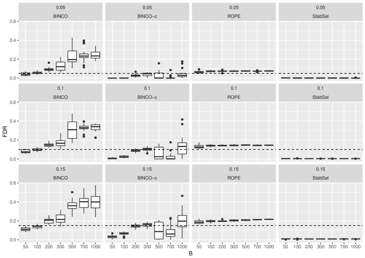
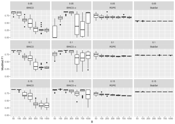
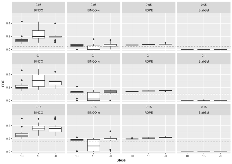
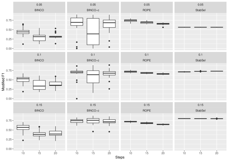
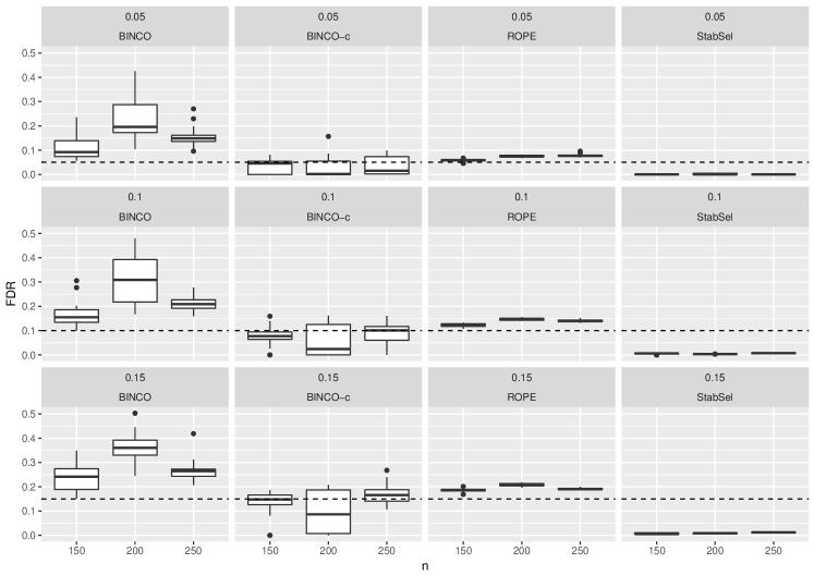
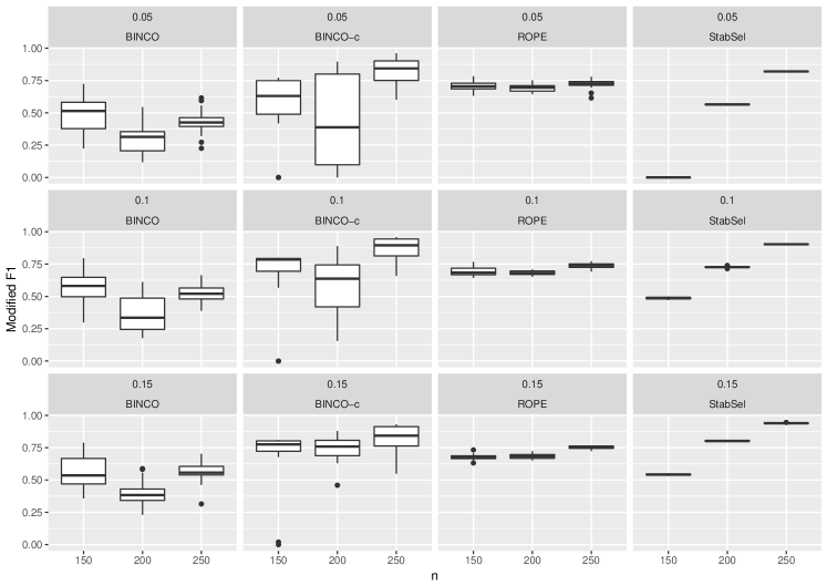
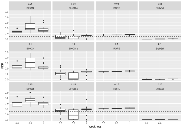
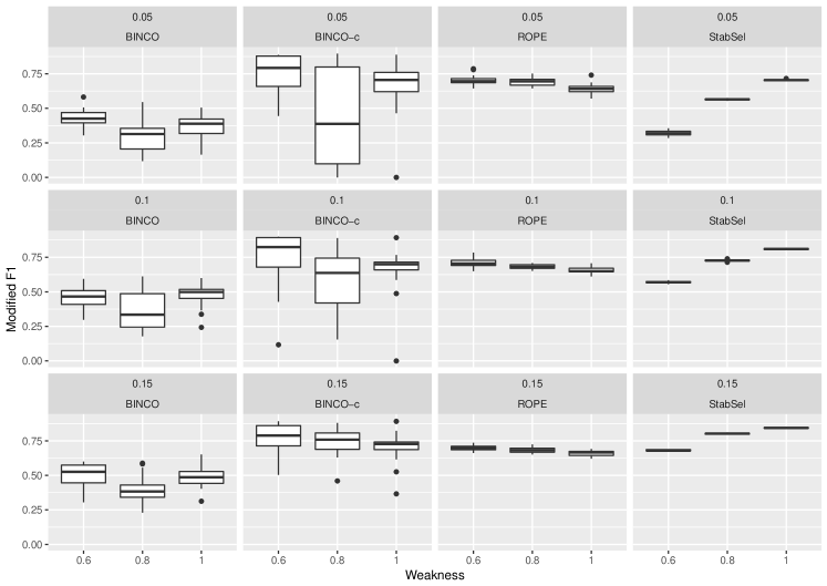
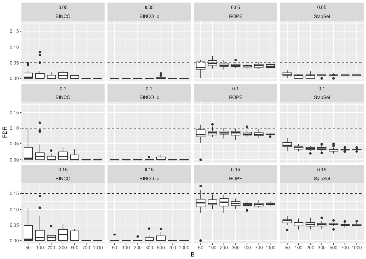
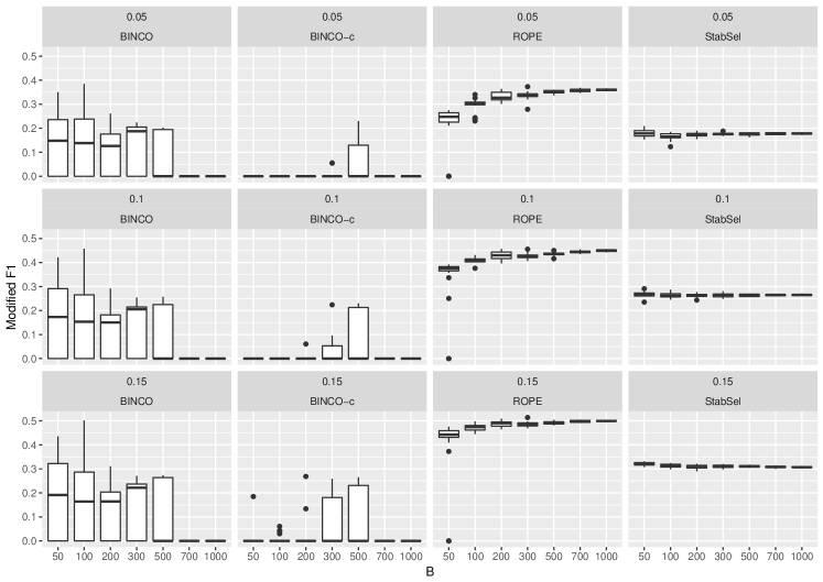
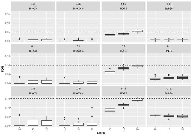
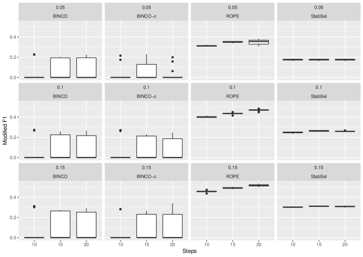
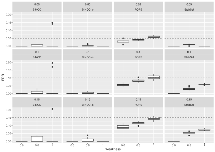
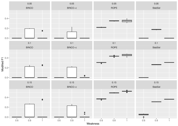
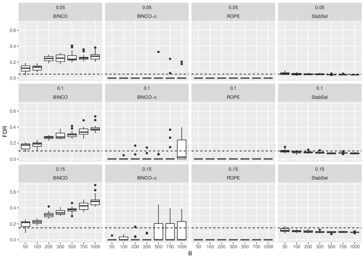
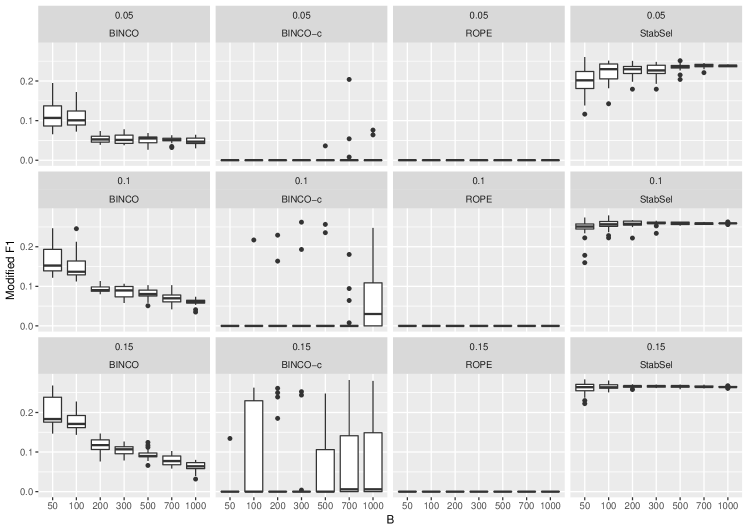
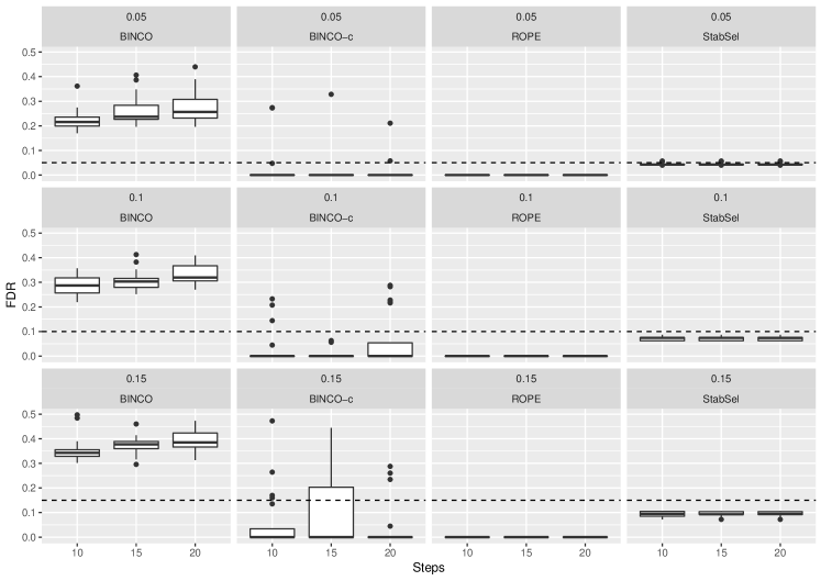
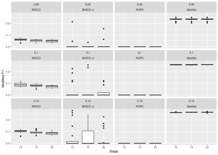
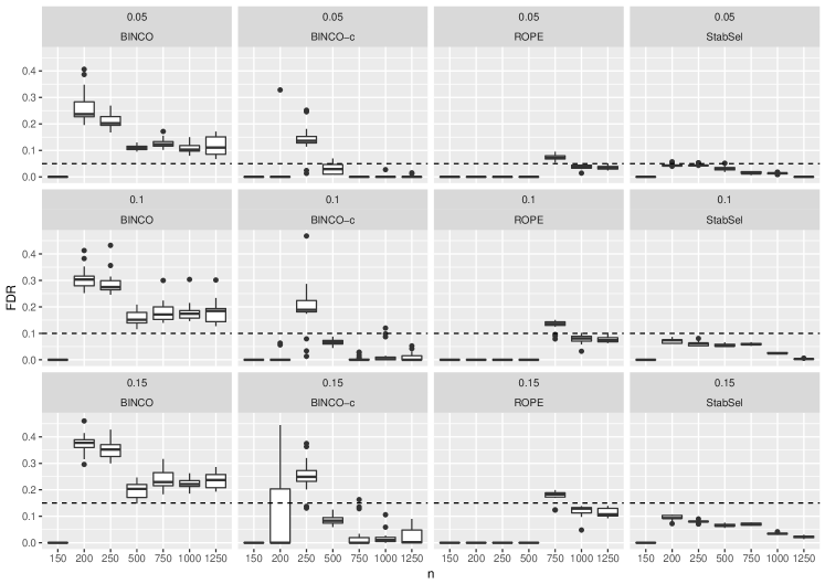
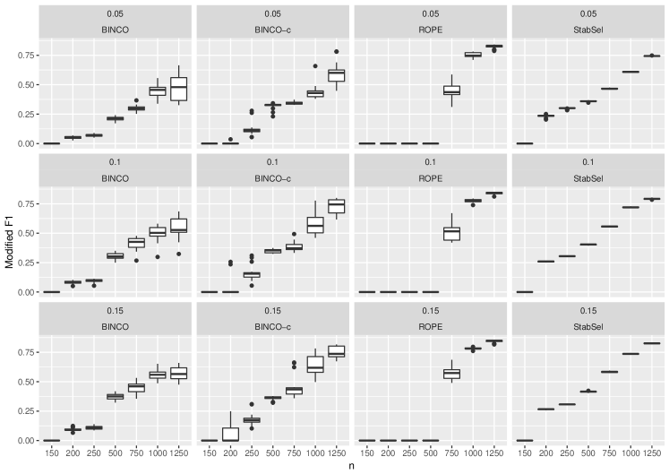
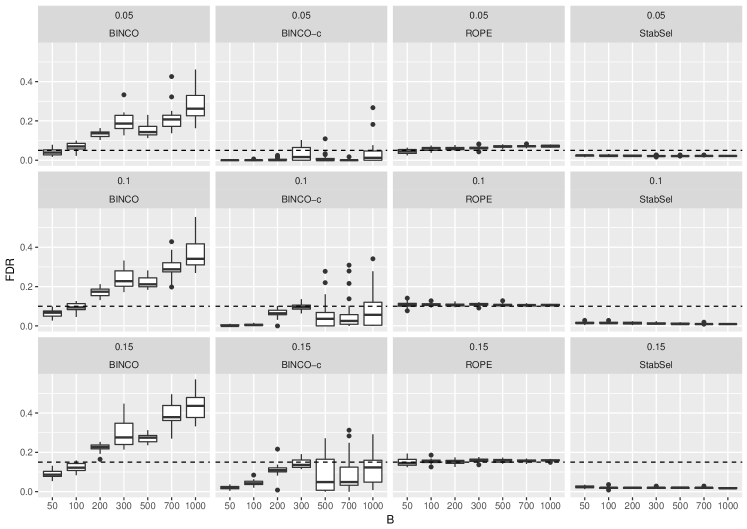
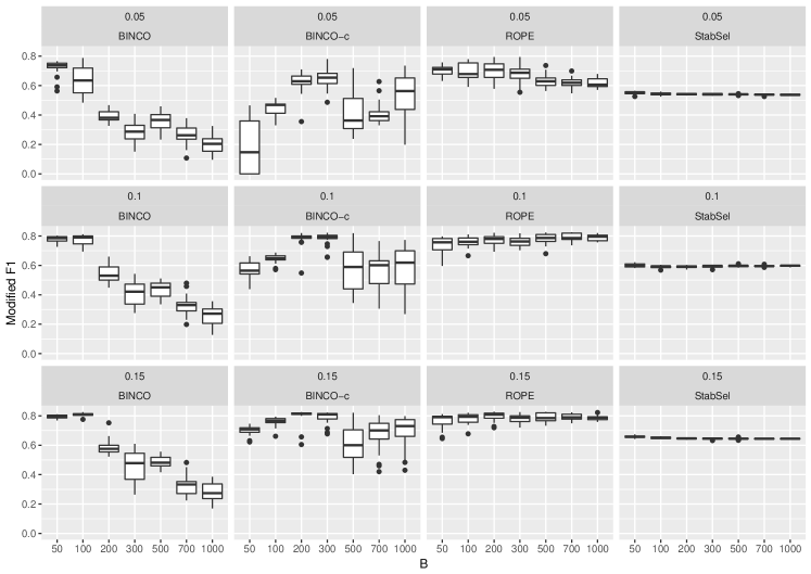
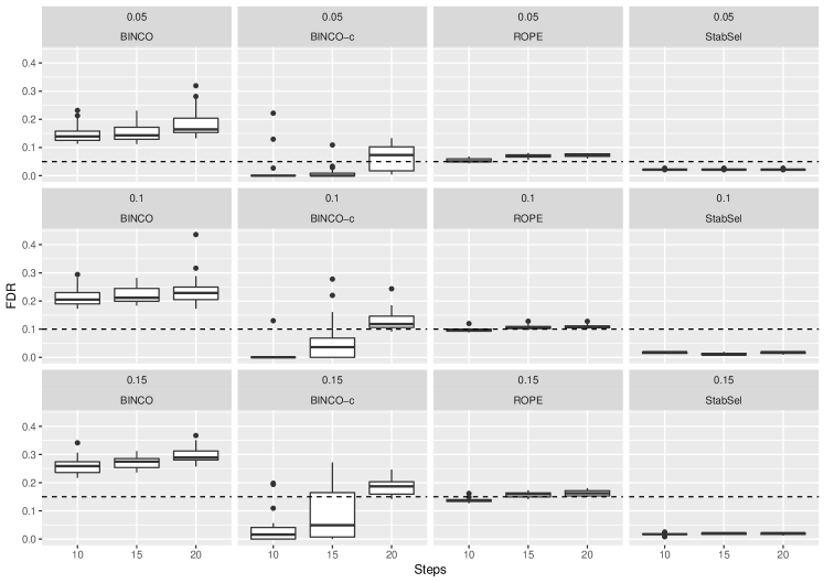
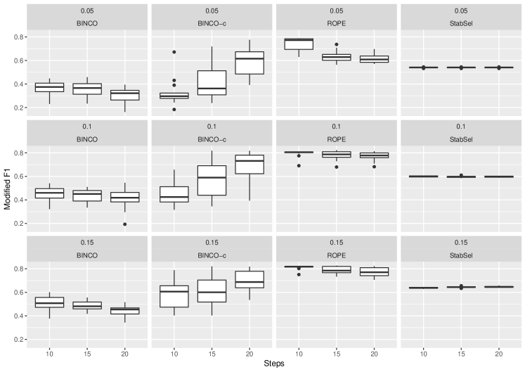
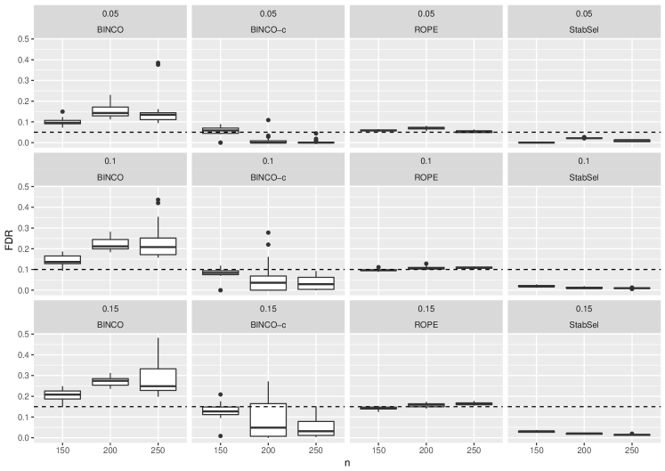
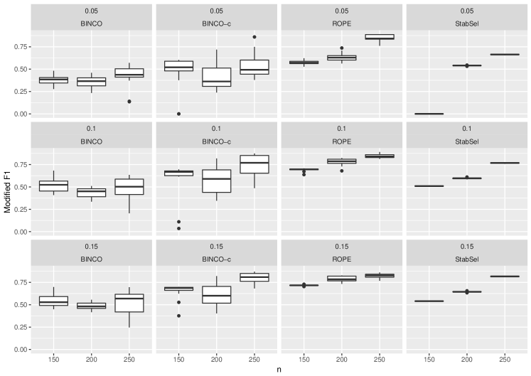
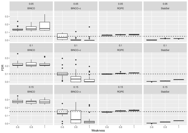
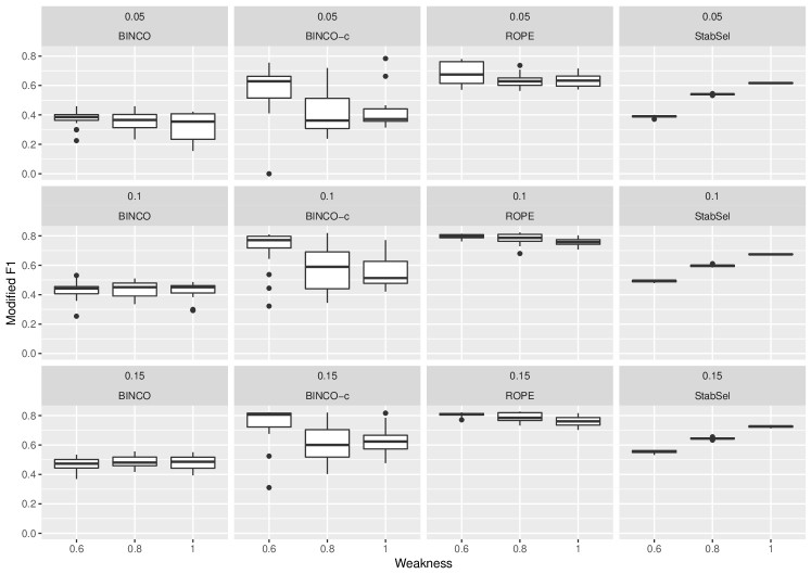
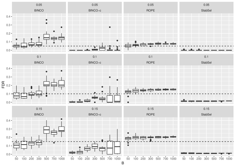
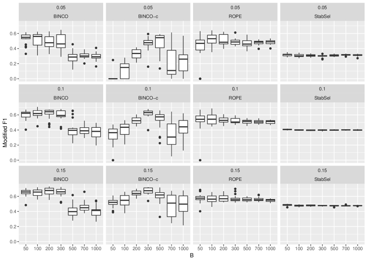
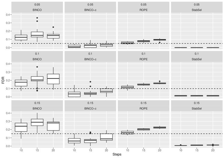
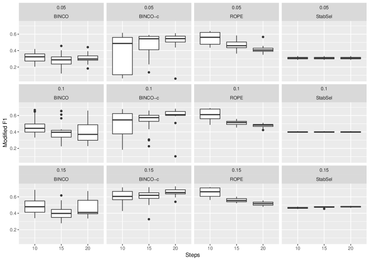
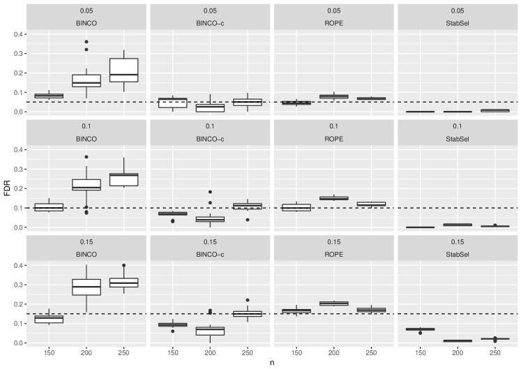
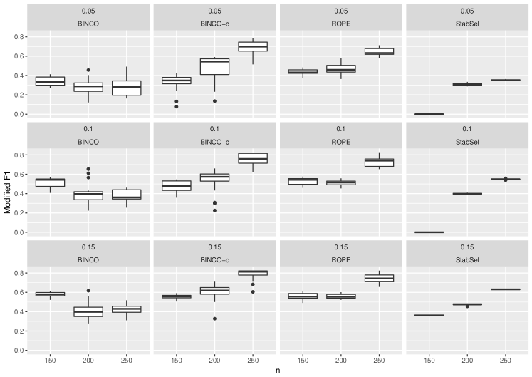
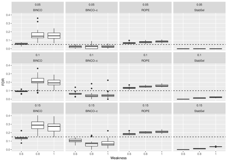
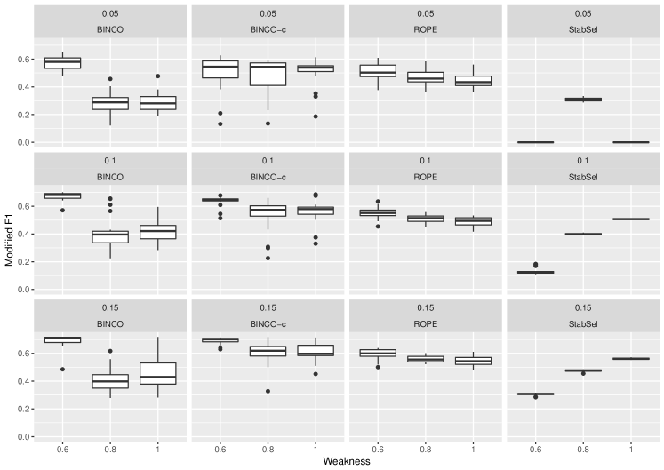
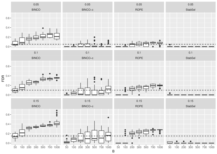
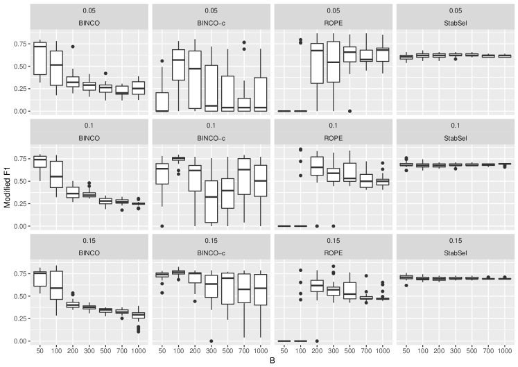
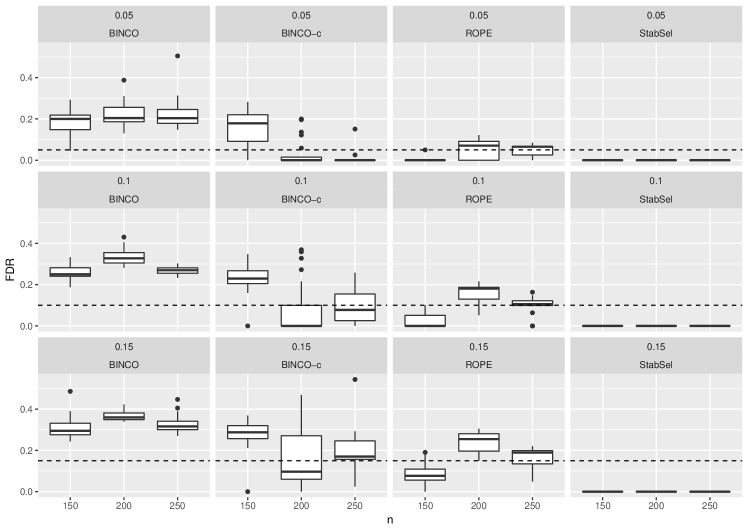
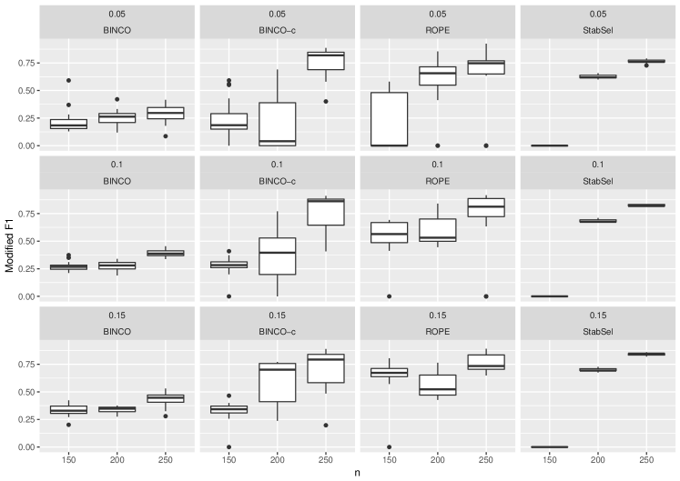
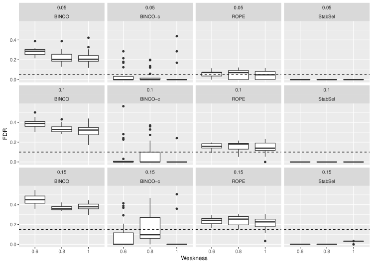
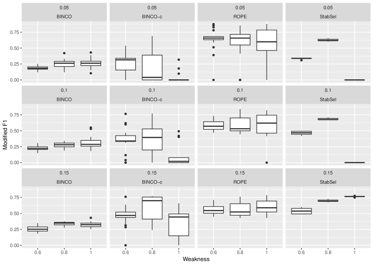
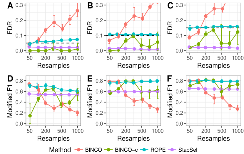
Results for the scale-free network with 500 nodes, 495 edges and strong signal is presented in Figures 2 and 3. In Figure 2, $B$ is varied, while $n=200$, weakness is 0.8 and $\Lambda$ consists of 15 steps. In Figure 3, $B=500$, while $n$, weakness and number of steps in $\Lambda$ is varied. Results for remaining topologies and parameter combinations are presented in the supplement.

Figure 4: Comparison of ROPE with and without joint modeling of counts from different penalization levels. When counts from different levels are used (Global) the estimated FDR is closer to the target FDR and the variance between simulations is lower.

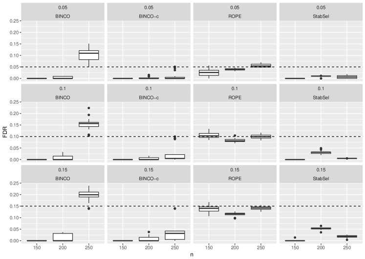
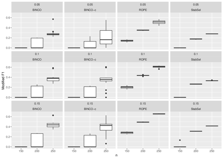
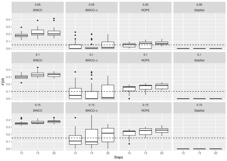
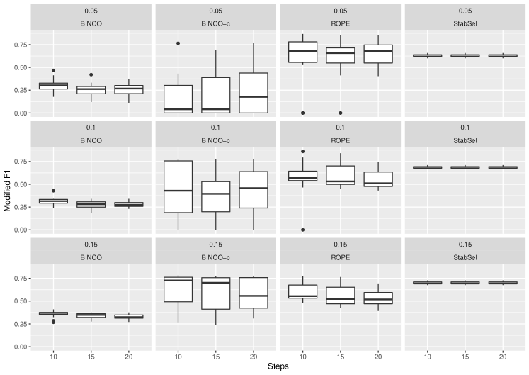
Results show that ROPE performs best in terms of modified F1, FDR and stability for the scale-free, dense scale-free, small scale-free and weak signal scale-free networks. In the chain network and the sparse scale-free network ROPE and stability selection perform similarly. Stability selection makes the most stable selections, but is generally too conservative, which is to be expected since the method is based on a bound. For the weak signal scale-free network and with a target FDR of 0.05, stability selection is too conservative to select any edge at all. BINCO and conservative BINCO both make far less stable selections than ROPE and stability selection. Furthermore, both BINCO methods are sensitive to the number of bootstraps. Logically, selection should improve when the number of bootstraps is increased. Instead, BINCO makes an increasingly more liberal selection. Similarly disconcerting, BINCO performance worsens with increased signal strength (number of observations) (Fig. 3A). Without access to the true model, it would be difficult to know how many bootstraps that should be performed to get a correct FDR control. This strong dependency between number of bootstraps, signal strength and achieved FDR makes BINCO hard to use in practice. The hubby network is the one setting where stability selection performs better than ROPE. There, ROPE makes no selection since the selection count histograms are not U-shaped. In order to examine how ROPE would perform for the hubby network if the signal were stronger, we generated additional observations, increasing the examined range from 150-500 observations to 150-1250 observations. For more than 500 observations, ROPE again yielded the highest modified F1 and the FDR closest to target.

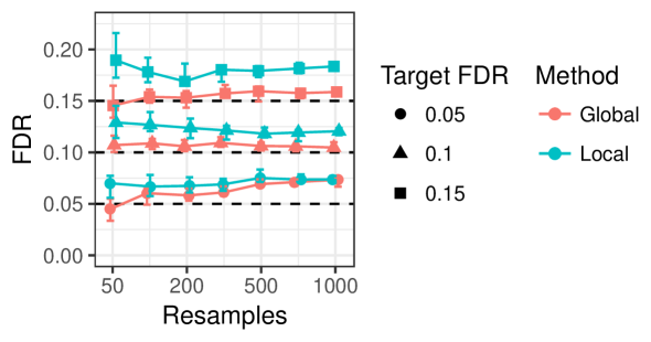
ROPE uses selection counts from several penalization levels and, as can be seen in Figure 4, this avoids a too liberal selection and increases stability. In addition, the Figure indicates that ROPE outperforms BINCO even without the joint modeling, which emphasizes the need to model both the null and non-null edge populations as done in ROPE.

In terms of computation time, BINCO and ROPE are slower than stability selection. At each level of penalization, ROPE fits a five parameter model, while BINCO estimates the end points of an approximately decreasing range and then fits three parameters. Both take only a few seconds per penalization level on a standard desktop computer. Increasing size of networks or the number of observations does not increase computation time, since these methods use summary statistics — the number of variables having a selection count $w$, for each $w\in\{0,\ldots,B\}$. The computation time of stability selection, BINCO and ROPE is small compared to the time needed for resampled variable selection.

3.2 FDR controlled edge selection for a graphical model of gene expressions in the PI3K/Akt pathway of glioblastoma cancer patients

Figure 5: ROPE selection of gene connections in the PI3K/Akt pathway based on gene expressions from glioblastoma cancer patients in TCGA. Widths of edges correspond to q-values. Highly connected nodes are known to have functions associated with invasiveness and/or tumor growth in glioblastoma.

Figure 6: Method comparison on gene expressions in the PI3K/Akt pathway of glioblastoma cancer patients. Panel A shows the number of selected edges by each method for a range of target FDR. While the achieved FDR is unknown, we note that BINCO is liberal enough to select more than 200 edges even at a low target FDR of 0.0125. As expected, stability selection is conservative producing empty networks for target FDR 0.25 and below. Conservative BINCO exhibits substantial variability in network size. Panel B shows agreement within each method across 20 subsamples of $W$ as measured by Fleiss’ $\kappa$. BINCO and conservative BINCO are less stable than ROPE and stability selection. The lack of agreement for BINCO at low targets combined with a large selection size, makes it unlikely that FDR is controlled. Fleiss’ $\kappa$ is not defined for empty selections produced by stability selection below FDR 0.25.

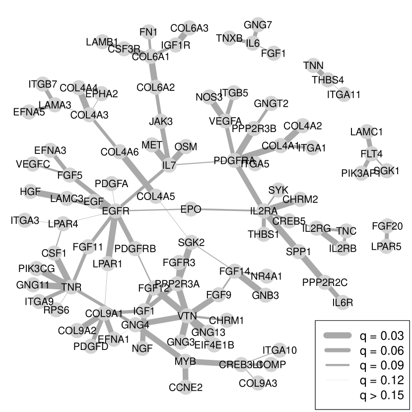
In this section, we apply ROPE to gene expression data and study the selected network. We also compare ROPE, BINCO and stability selection in terms of size of FDR controlled selections and stability. We downloaded RNA-Seq gene expressions for 172 glioblastoma multiforme cancer patients from the USCS Cancer Genomics Browser ¹⁶. The data comes from TCGA and had been normalized across all TCGA cohorts and log transformed. It contains measurements for 20,530 genes. We downloaded a list of genes in the PI3K/Akt signaling pathway from KEGG ¹⁷. 337 genes in the gene expression data set were found in the PI3K/Akt gene list. We discarded half of the genes with lowest median absolute deviation (MAD) of expression. Remaining genes were scaled to have MAD 1. We bootstrapped the data 500 times and estimated graphical models with 12 different levels of penalization for each bootstrap sample. The weakness in randomized lasso was set to 0.8. Figure 5 shows a visualization of the final network estimated with ROPE. In the visualization we have kept all edges with an estimated q-value below 0.15, i.e. we expect that 15% of the depicted edges are false discoveries. The edge widths correspond to estimated edge q-value. Zero degree nodes are not shown. Highly connected network nodes were the epidermal growth factor receptor (EGFR, 8 links), the platelet-derived growth factor receptor alpha (PDGRA, 6 links), components of the IL2 receptor (IL2RA and IL2RG, with 7 and 3 links), vitronectin (VTN, 7 links) and tenascin R (6 links). Of these, EGFR and PDGFRA are well established glioblastoma oncogenes. TNR is a tenascin with neural restricted expression, and is likely a negative marker of glioma invasiveness ¹⁸. By contrast VTN, which is connected to several FGF and FGFR isoforms in our network, is a pro-migratory/invasion factor ¹⁹. IL2, finally, has been suggested to promote growth of glioma cells ²⁰. Our network may thus serve to prioritize hub genes for further study, as well as their functionally associated genes. Edge q-values, along with properties of methodology for subsequent analysis, may facilitate the choice of how many associations to study further.

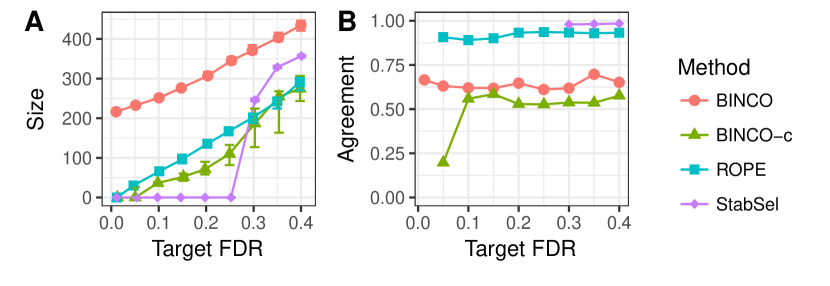
While the correct network model of the pathway is, of course, unknown, a comparison of methods on this real data shows relevant differences. We subsampled the 500 selected models 20 times without replacement. Each subsample consists of 400 selected models. Counting edge selections within each subsample gives 20 subsampled $W$. Figure 6 shows a comparison of size of FDR controlled selections and of stability of selections between subsamples. BINCO selects more than 200 edges already at a target FDR of 0.0125. Stability selection selects the empty model for target FDR 0.25 and below, in agreement with the conservative behaviour observed in the simulations. BINCO and conservative BINCO show more variation between selected models for different subsamples, than ROPE and stability selection. The liberal selection by BINCO agrees with simulation results, suggesting a failure to control FDR. BINCO’s lack of agreement between selections at low target FDR also suggests a failure to control FDR. The higher variability in BINCO and conservative BINCO also agrees with simulation results. We have used Fleiss’ $\kappa$, an index of inter-rater agreement among many raters ²¹, to measure agreement between selections across subsamples.

4 Discussion

The problem of FDR control in high-dimensional variable selection problems is of great relevance for interpreting data from molecular biology and other fields with an abundance of complex high-dimensional data. Many methods for variable selection in high-dimensional problems exist, but they suffer from the need to tune intermediate parameters of little scientific relevance. We have introduced a method for false discovery control in network models, and presented results showing that this method outperforms existing alternatives. With the method and software package presented here, which achieve accurate and robust FDR control, we have made possible a principled selection of relevant interactions.

We did consider an alternative statistical model for selection counts where the populations of alternative and null edges were further stratified into sub populations, based on their strength or the structure of their neighborhood in the graph. We did not find such a richer model to be worth the additional cost and estimation variability. Moreover, such a model poses the additional challenge of classifying each sub population as belonging to either the null or the alternative population. We also considered strengthening the connection between statistical models across all levels of penalization. Power and stability could potentially be increased by enforcing smoothness of all model parameters across levels of penalization. But the large number of edges that are represented in each histogram suggests that improvements would be small. Furthermore, the numerical fitting of such a global model is challenging.

ROPE, BINCO and stability selection use only summary statistics, proportions of variables with each selection count. Thus, their computational complexity is not affected by an increase in the number of network nodes. Computational time is completely dominated by the preceding step of resample based estimation. However, resampling based estimation is necessary to stabilize model selection and this process is parallelizable.

Recently, methods for assigning p-values to variables in high-dimensional linear models have been proposed. See ²² for a review and comparison. P-values can be used to approximate q-values ¹⁰, and thus to control FDR. Nevertheless, due to the high instability of estimated p-values (the so called “p-value lottery”) resampling is needed when applying the reviewed methods in practice ²². The application of this approach to graphical models is studied in ²³. ²⁴ proposes p-value estimation for linear models based a combination of the de-sparsified lasso and bootstrap. Here, the bootstrap is not used to aggregate many, unstable estimates but to improve on p-value estimates that relied on asymptotic arguments. The dependency on a penalization parameter remains (current implementation uses a fixed penalization chosen via cross-validation). ROPE can be applied to any resampling based network selection method, including resampling of p-value based selection, and could thus improve de-sparsified lasso estimates by utilizing multiple levels of penalization.

Here, ROPE was used for FDR controlled edge selection in a single penalization parameter setting. An interesting direction for future work would be to generalize ROPE to more complex modeling settings, e.g. comparative network modeling, with multiple tuning parameters. One could approach this problem in either a sequential fashion (across tuning parameters) or generalize the distribution mixture modeling to a higher-dimensional parameter space.

Lastly, the use of richer summaries of $W$ than histograms $h^{\lambda}$ may improve model selection. One way is to view edge presence counts $W^{\lambda}_{i}$ as functional data $W_{i}(\lambda)$. We have observed that these functions behave quite differently for different edges. The location and magnitude of $\min_{\lambda}\frac{d}{d\lambda}W_{i}(\lambda)$ are two examples of quantities that may facilitate edge selection. Another way is to consider correlation between edges. Edges can compete to explain the node correlation structure in a network neighborhood. Therefore, selection correlation between pairs of edges over resamples may also facilitate edge selection. Although computationally infeasible to estimate in full, the possibility to limit focus to edge pairs that are, in some sense, closely located in the network makes this an interesting direction of future research.

RJ and JK are supported in part by the Swedish Research Council. RJ is also supported in part by the Wallenberg foundation. SN is supported by the Swedish Research Council, Swedish Cancer Society and Swedish Childhood Cancer Foundation. AJ and JS are fulltime employees of Astra-Zeneca.

Conflict of interest: none declared.

Supplementary Materials

FDR controlled variable selection for a multinomial logistic regression classifier of gene expression profiles

In our final experiment, we apply ROPE to model selection for a non-graphical model. In particular, we demonstrate the use of ROPE for a multinomial logistic regression classifier for classifying the primary cancer type of a gene expression profile. We downloaded RNA-Seq gene expression profiles consisting of measurements of 20,530 genes for 9,755 cancer patients from the USCS Cancer Genomics Browser. The data comes from TCGA. We removed profiles corresponding to cancer types for which less than 100 observations were present in the data set, in order to reduce the chance of drawing bootstrap samples without all classes represented. The resulting data set consists of 9,256 observations and 20,530 variables. Each observation is classified as having one of 24 primary cancer types. We drew 100 bootstrap samples and fitted generalized linear models with lasso penalization and multinomial response to each bootstrap sample. We used grouped lasso penalization so that each variable is either selected for all classes or excluded entirely. For each bootstrap sample, one model was fitted for each of 22 levels of penalization, ranging from 0.015 to 0.039. Lower penalization resulted in non-convergence when fitting the model and higher penalization resulted in histograms not being U-shaped. The resulting matrix $W$ of 22 times 20,530 variable inclusion counts was used with ROPE to make an FDR controlled selection of genes whose expression level is predictive of primary cancer type. 86, 118 and 133 genes were selected at the 0.05, 0.1 and 0.15 FDR level, respectively. The selected genes are presented in Table 1. This experiment shows that ROPE can be applied to some variable selection problems other than edge selection in graphical models.

Additional simulation results

Figures below show results from all simulations. For each simulation setting, four parameters are varied one by one (number of bootstraps $B$, number of penalization levels, number of observations $n$ and weakness in randomized lasso). For each varied parameter, FDR and modified F1 are shown for each method and three target FDR: 0.05, 0.1 and 0.15. A detailed description of simulation settings and interpretation of results is given in the main article.

	gene	q-value		gene	q-value		gene	q-value
1	ATP5EP2	0.025	46	SFTA3	0.025	91	KRT74	0.051
2	AZGP1	0.025	47	SFTPA1	0.025	92	LYPLAL1	0.051
3	BCL2L15	0.025	48	SFTPB	0.025	93	MSX1	0.051
4	C10orf27	0.025	49	SLC6A3	0.025	94	MUC5B	0.051
5	C14orf105	0.025	50	SOX17	0.025	95	PTGER3	0.051
6	C8orf85	0.025	51	SPRYD5	0.025	96	RNF212	0.051
7	CALML3	0.025	52	ST6GALNAC1	0.025	97	SLC5A6	0.051
8	CDH16	0.025	53	TBX5	0.025	98	SLCO1A2	0.051
9	CDHR1	0.025	54	TCF21	0.025	99	C6orf223	0.058
10	CDX1	0.025	55	TFRC	0.025	100	ERBB3	0.058
11	CFHR2	0.025	56	TG	0.025	101	FOXF1	0.058
12	DPPA3	0.025	57	TMEFF2	0.025	102	IRX1	0.058
13	DSG3	0.025	58	TPO	0.025	103	NACAP1	0.058
14	EBF2	0.025	59	TRPS1	0.025	104	PHOX2A	0.058
15	EMX2	0.025	60	TSIX	0.025	105	C2orf80	0.065
16	FLJ45983	0.025	61	TYR	0.025	106	MMD2	0.065
17	FOXE1	0.025	62	UPK1B	0.025	107	SLC22A2	0.065
18	FTHL3	0.025	63	UPK2	0.025	108	APCS	0.071
19	FUNDC2P2	0.025	64	ZNF134	0.025	109	GJB1	0.071
20	FXYD2	0.025	65	ZNF280B	0.025	110	LOC285740	0.071
21	HAND2	0.025	66	FABP7	0.035	111	BCAR1	0.078
22	HOXA9	0.025	67	HOXC8	0.035	112	ACTC1	0.084
23	INS	0.025	68	KRT20	0.035	113	CTAGE1	0.091
24	IRX2	0.025	69	MAP7	0.035	114	ESR1	0.091
25	IRX5	0.025	70	MS4A3	0.035	115	GFAP	0.091
26	ITGA3	0.025	71	MUC16	0.035	116	HKDC1	0.091
27	KIAA1543	0.025	72	NOX1	0.035	117	PLA2G2F	0.091
28	KLK2	0.025	73	NTRK2	0.035	118	SOX10	0.091
29	LGSN	0.025	74	PAX3	0.035	119	PPARG	0.103
30	LOC407835	0.025	75	PRO1768	0.035	120	C21orf131	0.109
31	LOC643387	0.025	76	SERPINB3	0.035	121	DLX6	0.109
32	MAB21L2	0.025	77	SYCP2	0.035	122	GAL3ST3	0.109
33	NACA2	0.025	78	C14orf115	0.043	123	HNF1B	0.109
34	NDUFA4L2	0.025	79	C14orf19	0.043	124	KRT5	0.109
35	PA2G4P4	0.025	80	C1orf172	0.043	125	SPINK1	0.109
36	PAX8	0.025	81	FGL1	0.043	126	ARHGEF33	0.115
37	PHOX2B	0.025	82	GATA3	0.043	127	C1orf14	0.115
38	POU3F3	0.025	83	HOXA11	0.043	128	APOA2	0.121
39	PRAC	0.025	84	KRT7	0.043	129	LRRN4	0.121
40	RFX4	0.025	85	PRHOXNB	0.043	130	SOX2	0.121
41	RPL17	0.025	86	SCGB2A1	0.043	131	WNT3A	0.127
42	RPL39L	0.025	87	FLJ32063	0.051	132	GJB7	0.133
43	RPS4Y1	0.025	88	FOXA2	0.051	133	NASP	0.144
44	SCGB2A2	0.025	89	HECW2	0.051	134	ATCAY	0.150
45	SERPINB13	0.025	90	KLK3	0.051	135	DDR1	0.150

Table 1: The 135 transcripts with lowest q-value as selected with ROPE for a multinomial logistic classifier of expression profiles by cancer type.

Figure 7: Network topology: chain, steps: 15, $n=200$, weakness: 0.8, facet titles: target FDR and method.

Figure 8: Network topology: chain, steps: 15, $n=200$, weakness: 0.8, facet titles: target FDR and method.

Figure 9: Network topology: chain, $B=500$, $n=200$, weakness: 0.8, facet titles: target FDR and method.

Figure 10: Network topology: chain, $B=500$, $n=200$, weakness: 0.8, facet titles: target FDR and method.

Figure 11: Network topology: chain, $B=500$, steps: 15, weakness: 0.8, facet titles: target FDR and method.

Figure 12: Network topology: chain, $B=500$, steps: 15, weakness: 0.8, facet titles: target FDR and method.

Figure 13: Network topology: chain, $B=500$, steps: 15, $n=200$, facet titles: target FDR and method.

Figure 14: Network topology: chain, $B=500$, steps: 15, $n=200$, facet titles: target FDR and method.

Figure 15: Network topology: dense, steps: 15, $n=200$, weakness=0.8, facet titles: target FDR and method.

Figure 16: Network topology: dense, steps: 15, $n=200$, weakness=0.8, facet titles: target FDR and method.

Figure 17: Network topology: dense, $B=500$, $n=200$, weakness=0.8, facet titles: target FDR and method.

Figure 18: Network topology: dense, $B=500$, $n=200$, weakness=0.8, facet titles: target FDR and method.

Figure 19: Network topology: dense, $B=500$, steps:15, weakness=0.8, facet titles: target FDR and method.

Figure 20: Network topology: dense, $B=500$, steps:15, weakness=0.8, facet titles: target FDR and method.

Figure 21: Network topology: dense, $B=500$, steps:15, $n=200$, facet titles: target FDR and method.

Figure 22: Network topology: dense, $B=500$, steps:15, $n=200$, facet titles: target FDR and method.

Figure 23: Network topology: hubby, steps:15, $n=200$, weakness=0.8, facet titles: target FDR and method.

Figure 24: Network topology: hubby, steps:15, $n=200$, weakness=0.8 facet titles: target FDR and method.

Figure 25: Network topology: hubby, $B=500$, $n=200$, weakness=0.8, facet titles: target FDR and method.

Figure 26: Network topology: hubby, $B=500$, $n=200$, weakness=0.8 facet titles: target FDR and method.

Figure 27: Network topology: hubby, $B=500$, steps:15, weakness=0.8, facet titles: target FDR and method.

Figure 28: Network topology: hubby, $B=500$, steps:15, weakness=0.8, facet titles: target FDR and method.

Figure 29: Network topology: hubby, $B=500$, steps:15, $n=200$, facet titles: target FDR and method.

Figure 30: Network topology: hubby, $B=500$, steps:15, $n=200$, facet titles: target FDR and method.

Figure 31: Network topology: scale-free, steps:15, $n=200$, weakness=0.8, facet titles: target FDR and method.

Figure 32: Network topology: scale-free, steps:15, $n=200$, weakness=0.8, facet titles: target FDR and method.

Figure 33: Network topology: scale-free, $B=500$, $n=200$, weakness=0.8, facet titles: target FDR and method.

Figure 34: Network topology: scale-free, $B=500$, $n=200$, weakness=0.8, facet titles: target FDR and method.

Figure 35: Network topology: scale-free, $B=500$, steps:15, weakness=0.8, facet titles: target FDR and method.

Figure 36: Network topology: scale-free, $B=500$, steps:15, weakness=0.8, facet titles: target FDR and method.

Figure 37: Network topology: scale-free, $B=500$, steps:15, $n=200$, facet titles: target FDR and method.

Figure 38: Network topology: scale-free, $B=500$, steps:15, $n=200$, facet titles: target FDR and method.

Figure 39: Network topology: small, steps:15, $n=200$, weakness=0.8, facet titles: target FDR and method.

Figure 40: Network topology: small, steps:15, $n=200$, weakness=0.8, facet titles: target FDR and method.

Figure 41: Network topology: small, $B=500$, $n=200$, weakness=0.8, facet titles: target FDR and method.

Figure 42: Network topology: small, $B=500$, $n=200$, weakness=0.8, facet titles: target FDR and method.

Figure 43: Network topology: small, $B=500$, steps:15, weakness=0.8, facet titles: target FDR and method.

Figure 44: Network topology: small, $B=500$, steps:15, weakness=0.8, facet titles: target FDR and method.

Figure 45: Network topology: small, $B=500$, steps:15, $n=200$, facet titles: target FDR and method.

Figure 46: Network topology: small, $B=500$, steps:15, $n=200$, facet titles: target FDR and method.

Figure 47: Network topology: sparse, steps:15, $n=200$, weakness=0.8, facet titles: target FDR and method.

Figure 48: Network topology: sparse, steps:15, $n=200$, weakness=0.8, facet titles: target FDR and method.

Figure 49: Network topology: sparse, $B=500$, $n=200$, weakness=0.8, facet titles: target FDR and method.

Figure 50: Network topology: sparse, $B=500$, $n=200$, weakness=0.8, facet titles: target FDR and method.

Figure 51: Network topology: sparse, $B=500$, steps:15, weakness=0.8, facet titles: target FDR and method.

Figure 52: Network topology: sparse, $B=500$, steps:15, weakness=0.8, facet titles: target FDR and method.

Figure 53: Network topology: sparse, $B=500$, steps:15, $n=200$, facet titles: target FDR and method.

Figure 54: Network topology: sparse, $B=500$, steps:15, $n=200$, facet titles: target FDR and method.

References

- Pe’er and Hacohen 2011 Pe’er, D.; Hacohen, N. Cell 2011, 144, 864–873
- Kling et al. 2015 Kling, T.; Johansson, P.; Sánchez, J.; Marinescu, V. D.; Jörnsten, R.; Nelander, S. Nucleic Acids Research 2015,
- Friedman et al. 2008 Friedman, J.; Hastie, T.; Tibshirani, R. Biostatistics 2008, 9, 432–441
- Langfelder and Horvath 2008 Langfelder, P.; Horvath, S. BMC Bioinformatics 2008, 9, 559
- Margolin et al. 2006 Margolin, A. A.; Nemenman, I.; Basso, K.; Wiggins, C.; Stolovitzky, G.; Favera, R. D.; Califano, A. BMC Bioinformatics 2006, 7, S7
- Meinshausen and Bühlmann 2010 Meinshausen, N.; Bühlmann, P. Journal of the Royal Statistical Society: Series B (Statistical Methodology) 2010, 72, 417–473
- Liu et al. 2010 Liu, H.; Roeder, K.; Wasserman, L. Advances in Neural Information Processing Systems 23; 2010; pp 1432–1440
- Li et al. 2013 Li, S.; Hsu, L.; Peng, J.; Wang, P. Ann. Appl. Stat. 2013, 7, 391–417
- Bach 2008 Bach, F. R. Bolasso: model consistent lasso estimation through the bootstrap. Proc. of the 25th intl. conference on Machine learning. 2008; pp 33–40
- Storey and Tibshirani 2003 Storey, J.; Tibshirani, R. Proceedings of the National Academy of Sciences 2003, 100, 9440–9445
- The Cancer Genome Atlas Research Network et al. 2013 The Cancer Genome Atlas Research Network,; Weinstein, J.; Collisson, E.; Mills, G.; Shaw, K. M.; Ozenberger, B.; Ellrott, K.; Shmulevich, I.; Sander, C.; Stuart, J. Nat Genet 2013, 45, 1113–1120
- Jörnsten et al. 2011 Jörnsten, R.; Abenius, T.; Kling, T.; Schmidt, L.; Johansson, E.; Nordling, T. E. M.; Nordlander, B.; Sander, C.; Gennemark, P.; Funa, K.; Nilsson, B.; Lindahl, L.; Nelander, S. Molecular Systems Biology 2011, 7, 486
- Meinshausen and Bühlmann 2006 Meinshausen, N.; Bühlmann, P. Ann. Statist. 2006, 34, 1436–1462
- Zhao and Yu 2006 Zhao, P.; Yu, B. J. Mach. Learn. Res. 2006, 7, 2541–2563
- Efron 2004 Efron, B. Journal of the American Statistical Association 2004, 99, 96–104
- Goldman et al. 2014 Goldman, M.; Craft, B.; Swatloski, T.; Cline, M.; Morozova, O.; Diekhans, M.; Haussler, D.; Zhu, J. Nucleic Acids Research 2014,
- Kanehisa and Goto 2000 Kanehisa, M.; Goto, S. Nucleic acids research 2000, 28, 27–30
- Brösicke and Faissner 2015 Brösicke, N.; Faissner, A. Cell adhesion & migration 2015, 9, 131–140
- Ohnishi et al. 1998 Ohnishi, T.; Hiraga, S.; Izumoto, S.; Matsumura, H.; Kanemura, Y.; Arita, N.; Hayakawa, T. Clinical & experimental metastasis 1998, 16, 729–741
- Capelli et al. 1999 Capelli, E.; Civallero, M.; Barni, S.; Ceroni, M.; Nano, R. Anticancer research 1999, 19, 3147
- Fleiss 1971 Fleiss, J. L. Psychological bulletin 1971, 76, 378
- Dezeure et al. 2015 Dezeure, R.; Bühlmann, P.; Meier, L.; Meinshausen, N. Statist. Sci. 2015, 30, 533–558
- Janková and van de Geer 2015 Janková, J.; van de Geer, S. Electron. J. Statist. 2015, 9, 1205–1229
- Dezeure et al. 2016 Dezeure, R.; Bühlmann, P.; Zhang, C.-H. Preprint arXiv:1606.03940 2016,