Finding Strong Gravitational Lenses in the Kilo Degree Survey with Convolutional Neural Networks
Abstract
The volume of data that will be produced by new-generation surveys requires automatic classification methods to select and analyze sources. Indeed, this is the case for the search for strong gravitational lenses, where the population of the detectable lensed sources is only a very small fraction of the full source population. We apply for the first time a morphological classification method based on a Convolutional Neural Network (CNN) for recognizing strong gravitational lenses in square degrees of the Kilo Degree Survey (KiDS), one of the current-generation optical wide surveys. The CNN is currently optimized to recognize lenses with Einstein radii arcsec, about twice the -band seeing in KiDS. In a sample of colour-magnitude selected Luminous Red Galaxies (LRG), of which three are known lenses, the CNN retrieves 761 strong-lens candidates and correctly classifies two out of three of the known lenses. The misclassified lens has an Einstein radius below the range on which the algorithm is trained. We down-select the most reliable 56 candidates by a joint visual inspection. This final sample is presented and discussed. A conservative estimate based on our results shows that with our proposed method it should be possible to find massive LRG-galaxy lenses at in KiDS when completed. In the most optimistic scenario this number can grow considerably (to maximally 2400 lenses), when widening the colour-magnitude selection and training the CNN to recognize smaller image-separation lens systems.
keywords:
gravitational lensing: Strong – methods: statistical – galaxies: elliptical and lenticular, cD1 Introduction
Strong gravitational lensing is a rare phenomenon which provides very tight constraints on the projected mass of the foreground lens galaxy. In fact, the total mass (dark plus baryonic) within the Einstein radius depends almost solely on the space-time geometry of the lensing system (the source and the lens redshift and the cosmological parameters). For this reason, strong lensing is a unique tool, if combined with central velocity dispersion measurements and stellar population analysis, to estimate the fraction of dark matter in the central regions of galaxy-scale halos (e.g., Gavazzi et al. 2007; Jiang & Kochanek 2007; Grillo et al. 2010; Cardone et al. 2009; Cardone & Tortora 2010; Tortora et al. 2010; More et al. 2011; Ruff et al. 2011; Sonnenfeld et al. 2015), and to constrain the slope of the inner mass density profile (e.g., Treu & Koopmans 2002a, b; Koopmans et al. 2006; Koopmans & Treu 2003; More et al. 2008; Barnabè et al. 2009; Koopmans et al. 2009; Cao et al. 2016).
Gravitational lenses can be also used to constrain the stellar initial mass function (e.g., Treu et al. 2010; Ferreras et al. 2010; Spiniello et al. 2011; Brewer et al. 2012; Sonnenfeld et al. 2015; Posacki et al. 2015; Leier et al. 2016) and to independently measure the Hubble constant through time delays (e.g., Suyu et al. 2010; Bonvin et al. 2016). In addition, strong lensing gives magnified views of background objects otherwise inaccessible to observations (e.g., Impellizzeri et al. 2008; Swinbank et al. 2009; Richard et al. 2011; Deane et al. 2013; Treu et al. 2015; Mason et al. 2016).
A homogeneously selected large lens sample can improve dramatically the effectiveness of the methods and the reliability of the results from gravitational lensing studies. The largest homogeneous sample so far is provided by the Sloan Lens ACS Survey (SLACS; Bolton et al. 2008) with almost 100 observed lenses. In the future, deep high resolution wide surveys have the potential to produce samples three orders of magnitude larger than the current known lenses. These large numbers will allow to, e.g., greatly improve the precision in the mass density slope measurements (Barnabè et al., 2011), in better estimate the presence of substructure (Vegetti & Koopmans, 2009) and to put constraints on the nature of dark matter (Li et al., 2016).
Upcoming telescopes, such as Euclid (Laureijs et al., 2011) and the Large Synoptic Survey Telescope (LSST; LSST Science Collaboration et al. 2009), will increase the rate of discovery of new lenses, reaching the number of new strong lensing systems (Oguri & Marshall, 2010; Pawase et al., 2012; Collett, 2015). Also, the number of lenses that will be observed by the Square Kilometer Array is expected to be of the same of order of magnitude (McKean et al., 2015). The ongoing optical wide surveys, such as the Kilo Degree Survey (KiDS; see Sec. 2), the Dark Energy Survey (DES; The Dark Energy Survey Collaboration 2005) and the Subaru Hyper Suprime-Cam Survey (Miyazaki et al. 2012) are expected to find samples of lenses of the order of (see, e.g, Collett 2015). Sub-mm observations from Herschel (Negrello et al., 2010) and the South Pole Telescope (Carlstrom et al. 2011), together with deeper, high resolution observations from the the Atacama Large Millimeter/sub-millimeter Array, are expected to provide several hundred new lenses as well.
Traditionally, the search of extended lens features (i.e., arcs and rings) relied heavily on the visual inspection of the targets. This is still the best approach for small samples of objects, but is impractical for the ongoing and new generation surveys given the large number of targets that need to be inspected. Accordingly, numerous automatic lens finders have been developed in recent years. Most are based on the identification of arc-like shapes (e.g., Lenzen et al. 2004; Horesh et al. 2005; Alard 2006; Estrada et al. 2007; Seidel & Bartelmann 2007; Kubo & Dell’Antonio 2008; More et al. 2012). The same approach, together with a colour selection, is employed by Maturi et al. (2014). Another method consists of subtracting the light of the central galaxies using multiband images and then analyse the image residuals (Gavazzi et al., 2014). Joseph et al. (2014) follow a similar approach but employing machine-learning techniques to analyse single-band images. Instead Brault & Gavazzi (2015) model the probability that the targets are actual lenses. Very recently Bom et al. (2016) have developed an artificial neural network for recognizing strong lenses that uses as entries a set of morphological measurements of the targets. A completely different approach based on crouwdsourcing is employed in the Space Warps project (Marshall et al., 2016; More et al., 2016), with volunteers visually inspecting and classifying galaxy cutouts through a web applet111https://spacewarps.org/. All these automatic methods have their advantages and disadvantages and perform at their best with different typologies of lenses, quantity and kind of data available. A detailed comparison between these methods should be done on a common dataset, but is beyond the scope of this paper.
Convolutional Neural Networks (CNNs; Fukushima 1980; LeCun et al. 1998) are a state of the art class of machine learning algorithm particularly suitable for image recognition tasks. The ImageNet Large Scale Visual Recognition Competition (ILSVRC; Russakovsky et al. 2015; the most important image classification competition) of the last four years has been won by groups utilizing CNNs. The advantage of CNNs with respect to other pattern recognition algorithms is that they automatically define and extract representative features from the images during the learning process. Although the theoretical basis of CNNs was built in the the 1980s and the 1990s, only in the last years do CNNs generally outperform other algorithms due to to the advent of large labelled datasets, improved algorithms and faster training times on e.g. Graphics Processing Units (GPUs). We refer the interested reader to the reviews by Schmidhuber (2015), LeCun et al. (2015) and Guo et al. (2016) for a detailed introduction to CNNs.
The first application of CNNs to astronomical data was made by Hála (2014) for classifying spectra in the Sloan Digital Sky Survey (SDSS; Eisenstein et al. 2011). Then, Dieleman et al. (2015) 222The method won a challenge against other techniques https://www.kaggle.com/c/galaxy-zoo-the-galaxy-challenge/ used CNNs to morphological classify SDSS galaxies. Subsequently, Huertas-Company et al. (2015) used the same set-up of Dieleman et al. (2015) for classifying the morphology of high-z galaxies from the Cosmic Assembly Near-IR Deep Extragalactic Legacy Survey (Grogin et al., 2011). More recently, Hoyle (2016) adopted CNNs for estimating photometric redshifts of SDSS galaxies. CNNs have been employed also by Kim & Brunner (2016) for star/galaxy classification.
In this paper we present our morphological lens-finder which is based on CNNs. We apply it to the third data release of KiDS (de Jong et al., 2015, 2017), starting a systematic census of strong lenses. This project, which consists of both visual and automatic inspection of the KiDS images, is dubbed ”Lenses in KiDS” (LinKS). KiDS is a particularly suitable survey for finding strong lenses, given its excellent seeing and pixel scale, in addition to the large sky coverage (see Sect. 2).
The paper is organized as follows. In Sect. 2 we provide a brief description of the KiDS survey and the way in which we select the LRG-galaxy sample used in this work. In Sect. 3 we illustrate our lens-finding CNN-based algorithm and how we build the training data set. In Sect. 4 we explain how we apply our method to square degrees of KiDS, present the list of our new lens candidates, compare it with the literature and with a forecast of the expected number of detectable strong gravitational lenses in the survey and do a consistency check of the observed Einstein radii of the candidates to select the most reliable ones. Finally, in Sect. 5, we provide a summary, the main conclusion of this work and a short outlook for future plans and improvements. In the following we adopt a cosmological model with , where .
2 The KiDS survey
The Kilo-Degree Survey (KiDS) (de Jong et al., 2015) is one of the three ESO public surveys carried out using the OmegaCAM wide-field imager (Kuijken 2011) mounted at the Cassegrain focus of the VLT Survey Telescope (VST; Capaccioli & Schipani 2011) at Paranal Observatory in Chile. OmegaCAM is a 256 Megapixel camera containing 32 science CCD detectors which cover a one square degree field of view at a pixel-size of 0.21 arcsec. The VST is a 2.6m telescope with active control of the primary and secondary mirror which is driven by wave-front sensing via two auxiliary CCDs in OmegaCAM. In this way, the camera-telescope combination is specifically designed to obtain sharp and homogeneous image quality over the wide field of view. KiDS is a 1500 square degree extra-galactic imaging survey in four optical bands (, , and ). The survey area is divided over an equatorial patch and a Southern patch around the South Galactic Pole. Observations are queue scheduled, reserving the best seeing for the -band which has a median FWHM of the PSF of 0.65 arcsec with a maximum of 0.8 arcsec. Median PSF FWHM values in , and are 1.0 arcsec, 0.8 arcsec and 0.85 arcsec, respectively. KiDS reaches limiting magnitudes (5- AB in a 2 arcsec aperture) of 24.3, 25.1, 24.9 and 23.8 in , , and band, respectively. The primary science driver for the survey design is the study of the dark matter distribution over cosmological volumes via weak-lensing tomography. Strong-lensing survey studies are a particularly suitable science case as well, because they exploit the combination of superb image quality and wide survey area.
2.1 Data Release Three
In this paper we make use of the most recent public data release (KiDS ESO-DR3, de Jong et al. 2016, in prep). It consists of the co-added images, weight maps, masks, single-band and multi-band catalogues and photometric redshifts for 292 survey tiles. We use the multi-band photometry based on -band detections, with a total of 33 million unique sources. Our data handling and scientific data analysis is performed using the Astro-WISE information system (Valentijn et al., 2007). The source extraction and related photometry have been obtained with S-Extractor (Bertin & Arnouts 1996). We rely on both aperture photometry and the Kron-like MAG_AUTO. A relevant output parameter of S-Extractor is the FLAGS parameter. We set the -band FLAGS to be , to only include de-blended sources and remove from the catalogues those objects with incomplete or corrupted photometry, saturated pixels or any other kind of problem encountered during de-blending or extraction. Critical areas as saturated pixels, star spikes and reflection halos have been masked using a dedicated automatic procedure (Pulecenella). The IMA_FLAGS flags store the result of this masking operation: sources that are not in critical regions have this parameter set to 0. Photometric redshifts are determined using the program BPZ (Benítez 2000), which is a Bayesian photo- estimator based on a template fitting method (see de Jong et al. 2017, in prep., for further details). The unmasked effective area adopted, considering the sources with IMA_FLAGS in all the KiDS-DR3 bands, is 255 square degrees.
2.2 Luminous red galaxy sample
We select Luminous Red Galaxies (LRGs; Eisenstein
et al. 2001) from the 255 square degrees of the KiDS-ESO DR3 for the purpose of both training our CNN and searching for lens candidates among them. LRGs are very massive and hence more likely to exhibit lensing features compared to other classes of galaxies ( of the lensing population; see Turner
et al. 1984; Fukugita
et al. 1992; Kochanek 1996; Chae 2003; Oguri 2006; Möller et al. 2007). We focus on this kind of galaxies in this work and will consider other kind of galaxies in the future.
The selection is made with the following criteria where all the parameters are from S-Extractor and magnitudes are MAG_AUTO:
(i) The low- () LRG colour-magnitude selection of Eisenstein et al. (2001), adapted to including more sources (fainter and bluer):
| (1) |
(ii) A source size in the r-band larger than the average FWHM of the PSF of the respective tiles, times a empirical factor to maximize the separation between stars and galaxies.
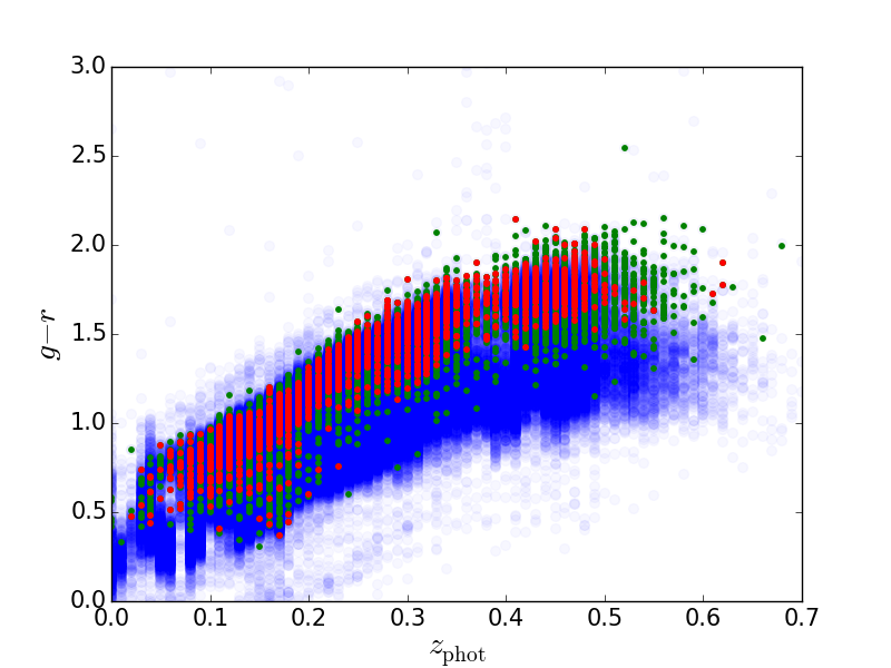
This final selection provides an average of 74 LRGs per tile and a total of 21789 LRGs. We refer to this sample as the ”LRG sample” in the remainder of the paper. Compared to the original colour-magnitude selection for (Eisenstein et al., 2001), we obtain times more galaxies. A colour-photo- diagram of the results of the two different cuts is shown in Fig. 1 for illustration.
3 Training the CNN to find Lenses
Our lens finder is based on a Convolutional Neural network (CNN) and is inspired by the work of Dieleman et al. (2015). CNNs are supervised deep learning algorithms (see the recent reviews from Schmidhuber 2015; LeCun et al. 2015; Guo et al. 2016) particularly effective for image recognition tasks (see e.g., He et al. 2015b, winner of the last ILSVRC competition; Russakovsky et al. 2015) and regression tasks, such as, in the astronomical domain, the determination of galaxy morphologies (Dieleman et al., 2015; Huertas-Company et al., 2015). The algorithm converts sequentially the input data through non-linear transformations whose parameters are learned in the training phase. A set of labelled images (the training set) are used as input of the CNN in this phase. The network changes its parameters by optimizing a loss function that expresses the difference between its output and the labels of the images in the training set. This allows the CNN to learn complex functions and to extract features from the data that are not hand designed but are learned during the training stage. After the training procedure the CNN can be used for classifying new data by keeping its parameters fixed. For the interested reader, in Appendix A we shortly introduce the technical background of CNNs that are relevant to some of the the choices made in this paper.
| Parameter | Range | Unit |
| Lens (SIE) | ||
| Einstein radius | 1.4 - 5.0 | arcsec |
| Axis ratio | 0.3 - 1.0 | - |
| Major-axis angle | 0.0 - 180 | degree |
| External shear | 0.0 - 0.05 | - |
| External-shear angle | 0.0 - 180 | degree |
| Source (Sérsic) | ||
| Effective radius | 0.2 - 0.6 | arcsec |
| Axis ratio | 0.3 - 1.0 | - |
| Major-axis angle | 0.0 - 180 | degree |
| Sérsic index | 0.5 - 5.0 | - |
3.1 Input Samples
Finding strong gravitational lenses can be reduced to a two-class classification problem, where the two kinds of objects to recognize are the lenses and the non-lenses. Training a Convolutional Neural Network (CNN) to solve this task requires a dataset representative of the two classes called training set. It has to be large enough because of the large number of parameters of a CNN (usually of the order of ). In the case of strong gravitational lenses we do not have a large enough representative data-set at our disposal. The largest sample available is collected in The Masterlens Database333http://masterlens.astro.utah.edu/. Unfortunately, this sample can not be used as a training set for our purpose, since it is small and heterogeneous. It consists of 657 lens systems that are not all spectroscopically confirmed, that have been discovered in various surveys and programs, or that are observed at different wavelengths according to the instrument used.
For these reasons, we build a set of mock lens systems, relying on a hybrid approach: first we select real galaxies, with their fields, obtained from KiDS (Sect. 3.1.1), in order to include seeing, noise and especially the lens environment that is a feature hard to simulate and its omission would limit the ability of the network to recognize lenses in real survey data. Then we independently simulate the lensed sources (Sect. 3.1.2) and combine them with the real galaxies (Sect. 3.2).
We limit our training to -band images, where KiDS provides the best image quality (an average FWHM of 0.65 arcsec). Hence, the network will learn selection criteria mostly based on the morphology of the sources. We plan to ingest multi-wavelength data into the network in future improvements, allowing the training on the differences in colours. Our training set consists of images of lens and non-lens examples produced with r-band KiDS images of real galaxies (see Sect. 3.1.1) and mock gravitational lensed sources (see Sect. 3.1.2). In Sect. 3.2 we summarize how the actual positive (lenses) and negative examples (non-lenses) employed in the training of the network, are produced. We train our CNN on a set of six millions images (three million lenses and three million non-lenses with labels 1 and 0, respectively). Our trained CNN gives as output a value ranging between 0 and 1. The sources with an output value of larger than 0.5 are classified as lenses. The technical details of our implementation and the training procedure can be found in Appendix B, providing further background to our procedures and choices. We further expand our training set using data augmentation techniques (Sect. 3.3).
3.1.1 Real Galaxy Sample
We select a sub-sample of the KiDS LRGs (see Sect. 2.2) consisting of 6554 galaxies (a third of the full sample), which we have visually inspected finding 218 contaminants, mostly face-on spirals. Additionally, we have collected a sample of 990 sources wrongly classified as lenses in previous tests with CNNs. We use this sample in the training set to reject clear outliers. The 6326 LRGs, the 218 contaminants and the 990 false positives constitute together the non-simulated part of the data used to build the training set. We will refer to it as the real galaxy sample in the remaining of this paper.
3.1.2 Mock Lensed-Source Sample
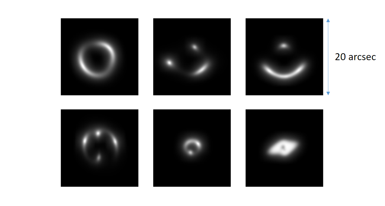
The mock lensed source sample is composed by simulated lensed images of 101 by 101 pixels, using the same spatial resolution of KiDS (0.21 arcsec per pixel), corresponding to a 20 by 20 arcsec field of view. We produce the different lensed image configurations by sampling uniformly the parameters of the lens and source models listed in Table 1. A few examples are shown in Fig. 2. The choice of uniformly sampling the parameter space does not reproduce the distribution of the parameters for a real lens population, but allows the classifier to learn the features for recognizing the different kinds of lenses, no matter how likely they are to appear in a real sample of lenses.
We model the sources with a Sersic (1968) profile and the lenses with a Singular Isothermal Ellipsoid (SIE; Kormann et al. 1994) model. At source redshifts of , smaller sizes and smaller Sérsic indices are found with respect to the local universe, and the fraction of spiral galaxies (with ) increases (e.g. Trujillo et al. 2007; Chevance et al. 2012). We exclude spiral galaxy sources or very elliptical ones considering only axis ratios . The source positions are chosen uniformly within the radial distance of the tangential caustics plus one effective radius of the source Sérsic profile. This leads our training set to be mostly composed of high-magnification rings, arcs, quads, folds and cusps rather than doubles (Schneider et al., 1992) that are harder to distinguish from companion galaxies and other environmental effects. In this paper our first-order goal is to find the larger, brighter and more magnified strong lenses, rather than aim for completeness over the full parameter space of lenses.
The upper limit of 5 arcsec for the Einstein radius aims to include typical Einstein radii for strong galaxy-galaxy and group-galaxy lenses (Koopmans et al. 2009; Foëx et al. 2013; Verdugo et al. 2014). The lower limit is chosen to be 1.4 arcsec, about twice the average FWHM of the r-band KiDS PSF. Because lenses are typically early-type galaxies, which do not have high ellipticity, we choose 0.3 as a lower limit of the axis ratio (Binney & Merrifield 1998). We set the external shear to less than 0.05, higher than typically found for SLACS lenses (Koopmans et al. 2006) with a random orientation varying between 0 and 180 degrees.
3.2 Building the training examples
Each training image passed to the network is built as described below and as summarized schematically in Fig. 3.
Mock lenses (positive sample):
To create the mock lenses we carry out the following procedure: (i) we randomly choose a mock lensed source from the mock source sample and a LRG from the real galaxy sample (Sections 3.1.2 and 3.1.1, respectively); (ii) we randomly perturb both the mock source and the LRG as described in Sect. 3.3; (iii) we rescale the peak brightness of the simulated source between 2% and 20% of the peak brightness of the LRG. In this way we take into account the typical lower magnitudes of the lensing features with respect to the lens galaxies despite the magnification; (iv) we add the two resulting images; (v) we clip the negative values of the pixels to zero and performing a square-root stretch of the image to emphasize lower luminosity features; and (vi) finally we normalize the resulting image by the peak brightness.
This procedure can yield a-typical lens configurations, because the mock sources and the KiDS galaxies are combined randomly, without taking into account the physical characteristics of the galaxies. Nevertheless, we operate in this way with the intent to train the network to classify a lens largely relying on the morphology of the source. Moreover, we reduce the risk of over-fitting, because the probability that the network will see twice the same (or a very similar) example is negligible. In addition, we cover the parameter space as free from priors as possible, which could allow to find less conventional lens configurations as well.
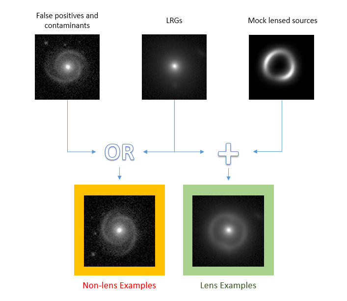
Non-lenses (negative sample): To create the mock non-lens sample we carry out the following procedure: (i) we randomly choose one galaxy from the real galaxy sample (see Sect. 3.1.1) with a 60% probability of extracting a LRG and 40% probability to extract a contaminant or false positive; (ii) we randomly perturbing as in Sect. 3.3; (iii) we apply a square-root stretch of the image; (iv) we normalizing the image by the peak brightness.
The final inputs of the convolutional neural network are image-cutouts of 60 by 60 pixels which correspond to by 12 arcsec. These images are produced in real-time during the training phase.
3.3 Data augmentation
A common practice in machine learning is data augmentation: a procedure used to expand the training set in order to avoid over-fitting the data and teaching the network rotational, translational and scaling invariance (see e.g., Simard et al. 2003). We augment our dataset applying the following transformations to the mock lensed images and the real galaxy sample: (i) a random rotation between 0 and ; (ii) a random shift in both and direction between -4 and +4 pixels; (iii) a probability of horizontally flipping the image; (iv) a rescaling with a scale factor sampled log-uniformly between and . All transformations are applied to the image-cutouts of 101 by 101 pixels of both the real galaxy and mock lensed source sample. We extract a central region of 60 by 60 pixels from the resulting images to avoid unnecessarily information (i.e., noise and empty sky) around the image edges.
4 Results
Having trained the CNN as described in Sect. 3 (see also Appendix B for more details), in this section we present our results. In Sect. 4.1 we report the procedure to select our final sample of lens candidates and in Sect. 4.2 the sample is presented, discussed and compared with the literature.
4.1 Candidate selection
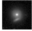
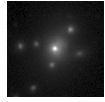
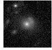
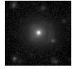
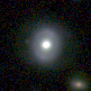
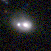
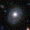
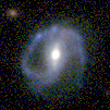
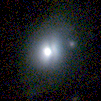
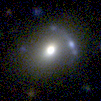
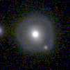
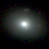
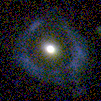
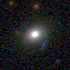
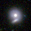
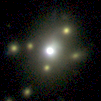
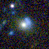
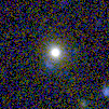
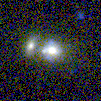
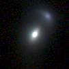
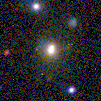
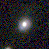
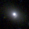
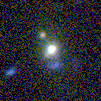
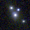
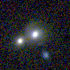
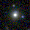
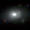
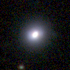
First we ingest the full 21789 LRG sample (see Sect. 2.2) in to the trained CNN. We obtain 761 galaxies ( of the full LRG sample) classified as lens candidate with and all the remainder in the non-lens category with with . The number of LRG classified by the network as lenses is too large when compared to the expected number of strong lenses in the KiDS-DR3 area (see Sect. 4.2.1). Among the selected sources there are contaminants such as spirals, galaxies with dust lanes, mergers, etc. (see Fig. 4 for some examples). For this reason we decide to further visually classify the 761 targets selected by the network. Seven of the authors of this paper – referred as “classifiers” in the following – are presented with a set of images for each lens candidate: the cut-out images from KiDS (one image per each of the u, g, r, and i filters) and a RGB reconstructed composite image obtained with the software STIFF444http://www.astromatic.net/software/stiff from the g, r, and i-band images.
The classifiers can classify the sources in three categories: Sure, Maybe, and No lens. The score for each candidate is based on the following scheme:
| Sure lens | 10 points. |
| Maybe lens | 4 points. |
| No lens | 0 points. |
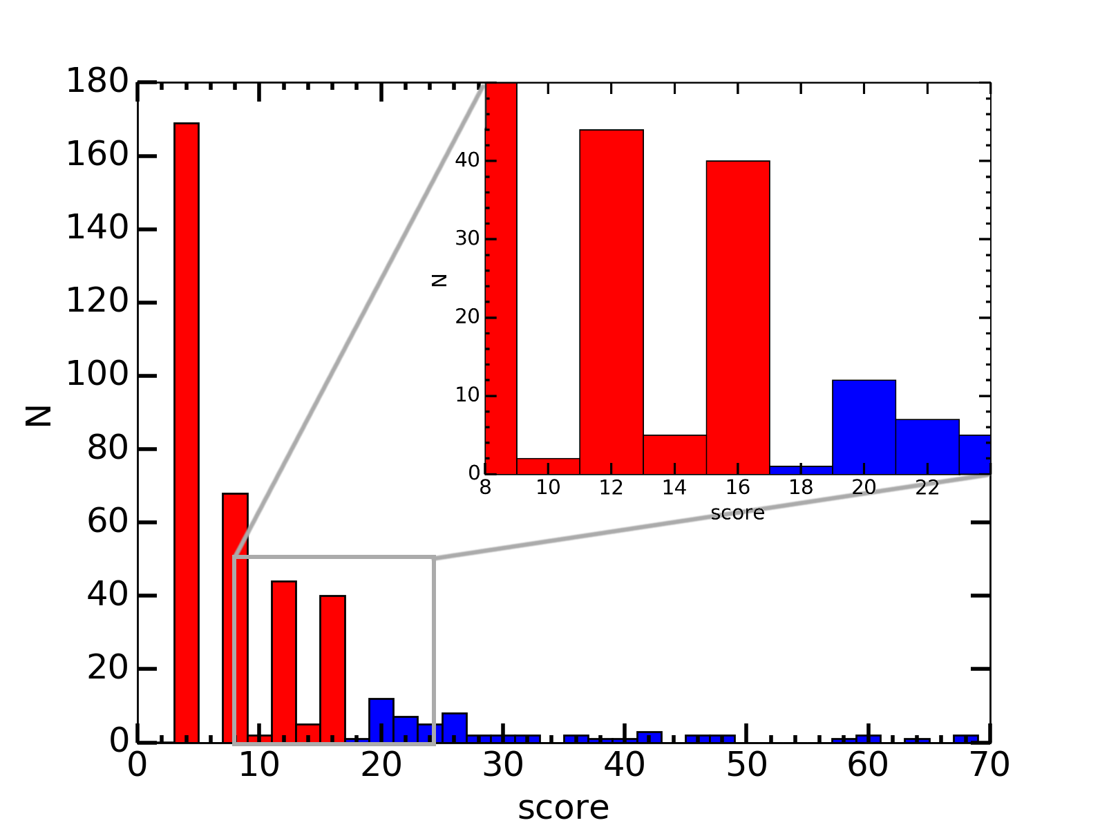
The histogram of the accumulated grades of the visual classification is shown in Fig. 5. There are 384 candidates classified in the Sure and Maybe categories by at least one classifier. To further reduce the sample, we decide to introduce a threshold at the score of 17, below which all candidates are considered not reliable. This implies that more than four classifiers would be required to classify a lens candidate in the Maybe category to be regarded as reliable. For lenses in the Sure category we expect a large number of users to agree in their classification due to more evident lensing features in the images, giving a higher score to such candidates. Only two candidates achieved the maximum score of 70. As seen in Fig. 5 (blue bars), the distribution of candidates rises rapidly below the threshold score and remains flat for higher values. Changing the points given to a candidate classified as Maybe lens from four to six, and appropriately relocating the threshold, does not affect the resulting ranking, and the distribution shown in Fig. 5 remains largely the same.
Since the focus of this paper is to find new lens candidates, we are interested in the first two categories, i.e. Sure and Maybe. However, we plan for future applications to use the candidates classified in the No category to retrain the CNN, aiming at considerably reducing the number of candidates that need to be visually inspected.
4.2 Final sample of candidates
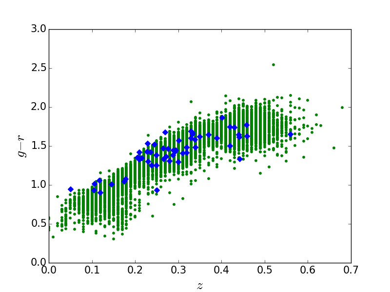
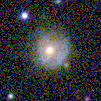
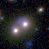
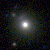
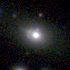
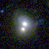
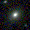
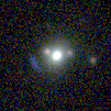
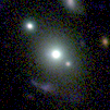
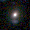
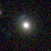
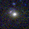
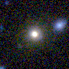
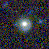
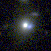
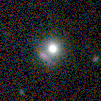
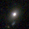
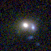
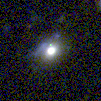
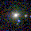
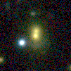
After both CNN and visual classification, the final sample of lens candidates consists of 56 objects, down-selected from an initial sample of 21789 galaxies. In Fig. 6 we show how the candidates are distributed in colour-photo- space together with the full LRG sample (Sect. 2.2). In Fig. 11 the RGB images of these best candidates are shown together with their scores from the visual inspection procedure. For completeness, in Appendix C the r-band-only images of the 56 ranked objects are also shown, since they are the images on which the CNN has made its classification. Candidates are listed in Table 2, where we show the final grade of our classification, the KiDS MAG_AUTO in the u, g, r, and i bands for each candidate, together with the BPZ photometric redshift, stellar mass and, if available, spectroscopic redshift and velocity dispersion.
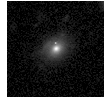
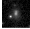
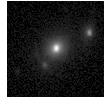
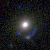
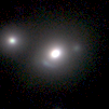
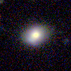
J085446-012137 and J114330-014427 are successfully classified as lenses by our network and they pass our visual inspection with a score of 70 and 60 respectively (KSL317 and KSL040 in Table 2 and Fig. 11). Instead, J1403+0006 is classified as a non-lens by the network, this could be due to the fact that this system has an Einstein radius of 0.83 arcsec, well below the lower limit of the interval of radii on which the CNN is trained. In Fig. 7 we show the RGB images of these three known lenses as observed in KiDS. The lensed images of the misclassified lens are also not as prominent as in the other two.
We find that 34 of our candidates have spectra measured from different sources (2dF, Colless et al. 2001; Limousin et al. 2010; SDSS, Eisenstein et al. 2011; BOSS, Dawson et al. 2013; GAMA, Liske et al. 2015). We visually inspected the spectra without clearly identifying any emission line that could belong to a background source. A more detailed data reduction of the spectra is needed to confirm or discard any of these candidates. We also notice that the photometric redshifts tend to overestimate the distance. This could be due to the contamination of the colours of the main galaxy by the supposed lensed sources. We will investigate this issue in a forthcoming paper.
| ID | [km/s] | [dex] | score | |||||||
|---|---|---|---|---|---|---|---|---|---|---|
| KSL427 | 0.25 | 20.17 | 18.38 | 16.96 | 16.58 | 11.3 | 70 | |||
| KSL317 | 0.42 | 21.43 | 19.61 | 17.86 | 17.20 | 11.6 | 70 | |||
| KSL103 | 0.26 | 20.55 | 18.53 | 17.28 | 16.81 | 11.3 | 64 | |||
| KSL040 | 0.15 | 18.56 | 16.65 | 15.64 | 15.26 | 11.1 | 60 | |||
| KSL627 | 0.24 | 20.89 | 18.75 | 17.42 | 16.92 | 11.3 | 60 | |||
| KSL327 | 0.17 | 18.96 | 16.80 | 15.75 | 15.33 | 11.4 | 58 | |||
| KSL376 | 0.36 | 21.88 | 20.03 | 18.46 | 17.91 | 11.2 | 48 | |||
| KSL086 | 0.33 | 22.30 | 20.23 | 18.54 | 18.03 | 11.1 | 48 | |||
| KSL351 | 0.30 | 21.12 | 18.89 | 17.42 | 16.91 | 11.4 | 46 | |||
| KSL469 | 0.33 | 21.23 | 19.52 | 18.08 | 17.51 | 11.4 | 46 | |||
| KSL228 | 0.16 | 19.83 | 18.30 | 17.25 | 16.75 | 11.2 | 42 | |||
| KSL713 | 0.29 | 20.46 | 18.54 | 17.01 | 16.47 | 11.5 | 42 | |||
| KSL328 | 0.24 | 21.28 | 19.52 | 18.09 | 17.58 | 11.0 | 42 | |||
| KSL411 | 0.27 | 18.62 | 17.59 | 16.66 | 16.22 | 11.5 | 40 | |||
| KSL070 | 0.45 | 21.55 | 20.37 | 19.05 | 18.37 | 11.2 | 40 | |||
| KSL543 | 0.25 | 20.73 | 19.03 | 17.78 | 17.29 | 11.3 | 38 | |||
| KSL664 | 0.30 | 21.89 | 19.91 | 18.62 | 18.00 | 11.1 | 36 | |||
| KSL106 | 0.28 | 21.75 | 19.96 | 18.59 | 18.06 | 11.1 | 36 | |||
| KSL337 | 0.35 | 22.06 | 20.55 | 18.93 | 18.41 | 10.8 | 32 | |||
| KSL388 | 0.37 | 22.83 | 19.81 | 18.14 | 17.58 | 11.4 | 32 | |||
| KSL415 | 0.21 | 20.64 | 19.03 | 17.68 | 17.19 | 11.3 | 32 | |||
| KSL220 | 0.31 | 21.85 | 20.32 | 18.91 | 18.42 | 11.2 | 30 | |||
| KSL601 | 0.54 | 23.09 | 21.41 | 19.65 | 18.97 | 11.1 | 28 | |||
| KSL603 | 0.41 | 21.96 | 20.04 | 18.46 | 17.86 | 11.5 | 28 | |||
| KSL436 | 0.27 | 21.44 | 19.57 | 17.90 | 17.74 | 10.8 | 26 | |||
| KSL233 | 0.17 | 19.96 | 18.17 | 17.16 | 16.67 | 10.8 | 26 | |||
| KSL231 | 0.46 | 23.73 | 20.98 | 19.36 | 18.64 | 11.3 | 26 | |||
| KSL101 | 0.32 | 22.92 | 20.36 | 18.89 | 18.33 | 11.2 | 26 | |||
| KSL450 | 0.46 | 23.24 | 20.83 | 18.97 | 18.44 | 11.2 | 26 | |||
| KSL737 | 0.45 | 22.27 | 20.39 | 18.74 | 18.14 | 11.4 | 26 | |||
| KSL094 | 0.42 | 20.77 | 19.36 | 17.94 | 17.37 | 11.5 | 26 | |||
| KSL669 | 0.16 | 19.46 | 17.58 | 16.63 | 16.17 | 10.4 | 26 | |||
| KSL707 | 0.25 | 21.77 | 19.66 | 18.28 | 17.72 | 11.0 | 24 | |||
| KSL197 | 0.21 | 21.63 | 19.56 | 18.14 | 17.71 | 11.1 | 24 | |||
| KSL335 | 0.26 | 21.89 | 19.07 | 17.72 | 17.19 | 11.2 | 24 | |||
| KSL565 | 0.29 | 21.52 | 19.97 | 18.52 | 17.97 | 11.1 | 24 | |||
| KSL134 | 0.29 | 21.23 | 19.57 | 18.24 | 17.73 | 11.3 | 24 | |||
| KSL606 | 0.17 | 19.79 | 18.32 | 17.25 | 16.85 | 11.2 | 22 | |||
| KSL046 | 0.12 | 18.44 | 16.69 | 15.79 | 15.40 | 11.4 | 22 | |||
| KSL620 | 0.28 | 21.53 | 19.78 | 18.47 | 17.91 | 11.1 | 22 | |||
| KSL013 | 0.14 | 19.73 | 18.19 | 17.26 | 16.74 | 10.7 | 22 | |||
| KSL421 | 0.32 | 21.42 | 19.65 | 18.23 | 17.69 | 11.4 | 22 | |||
| KSL434 | 0.39 | 21.74 | 20.06 | 18.47 | 17.99 | 11.0 | 22 | |||
| KSL516 | 0.56 | 23.33 | 21.19 | 19.55 | 18.80 | 11.1 | 20 | |||
| KSL278 | 0.42 | 21.85 | 20.34 | 18.84 | 18.32 | 11.2 | 20 | |||
| KSL178 | 0.43 | 21.74 | 20.04 | 18.31 | 17.63 | 11.9 | 20 | |||
| KSL159 | 0.44 | 22.08 | 20.32 | 18.68 | 18.08 | 11.7 | 20 | |||
| KSL686 | 0.30 | 21.77 | 19.24 | 17.72 | 17.20 | 11.2 | 20 | |||
| KSL465 | 0.34 | 20.49 | 19.17 | 17.69 | 17.17 | 11.6 | 20 | |||
| KSL463 | 0.23 | 21.24 | 19.61 | 18.31 | 17.85 | 10.8 | 20 | |||
| KSL342 | 0.21 | 21.22 | 19.28 | 17.95 | 17.49 | 10.9 | 20 | |||
| KSL322 | 0.44 | 22.27 | 20.02 | 18.37 | 17.76 | 11.5 | 20 | |||
| KSL674 | 0.31 | 21.68 | 19.60 | 18.14 | 17.60 | 11.2 | 20 | |||
| KSL564 | 0.33 | 22.92 | 19.85 | 18.47 | 17.88 | 11.2 | 20 | |||
| KSL670 | 0.48 | 23.71 | 21.10 | 19.49 | 18.72 | 11.4 | 20 | |||
| KSL535 | 0.44 | 22.08 | 20.32 | 18.68 | 18.08 | 11.5 | 18 |
4.2.1 Expected number of lenses
To assess whether the amount of selected candidates is reliable, we estimate the detectable lens population in KiDS, using the lens-statistics code LensPop555https://github.com/tcollett/LensPop (Collett, 2015). Assuming an effective KiDS survey area of sq. deg we forecast potentially detectable lenses with a total signal-to-noise ratio larger than 20 and having lensed images resolved over least three seeing elements. The expected number of lenses reduces to for the effective area of the KiDS-DR3 of sq. deg. If we consider only lenses that satisfy our colour-magnitude cut of Sect. 2.2 and with an Einstein radius arcsec, i.e., our range of the parameter space, we forecast lenses for sq. deg, broadly comparable to the number of our final sample of candidates, especially if we keep in mind that (i) we do not expect the CNN plus human lens selection to be 100% efficient and (ii) our training was largely focused on arcs and rings and not on quads and doubles. The redshift distribution of our final sample of candidates and the simulated population from LensPop, within the selection constraints specified above, are also consistent. Our candidates are observed in the window , with a median redshift of , while the LensPop sample is in the window with a median redshift of . The scatter corresponds to the 16-84th quantiles of the distribution.
4.3 Sample Characterization and Comparison
To further characterize the sample of candidates, and allow a comparison with the literature, we estimate the stellar masses using the software Le Phare (Arnouts et al. 1999; Ilbert et al. 2006), which performs a fitting between the stellar population synthesis (SPS) theoretical models and the data. Single burst models from Bruzual & Charlot (2003, BC03) and a Chabrier (2001) IMF are implemented in the software. In the BC03 models we leave the age free to vary up to a maximum of , and assume metallicities in the range (0.005–2.5 ). No internal extinction is adopted. The single burst models provide us with a fair description of the stellar populations in massive early-type galaxies. Models are redshifted using the photometric redshifts (or the spectroscopic estimates where available). We adopt the observed magnitudes (and related uncertainties) within a arcsec diameter aperture, corrected for Galactic extinction using the map in Schlafly & Finkbeiner (2011)666These updated extinctions are calculated by multiplying for 0.86 the Schlegel et al. (1998) values stored in the KiDS-DR3 catalog.. The r-band MAG_AUTO is used to correct the outcomes of Le Phare for missing flux. For 34 out of the 56 lens candidates (i.e., 60 per cent) we have spectroscopic redshifts. As pointed out previously, photometric redshifts tend to be larger than the spectroscopic estimate by , on average. For the 22 galaxies with a photometric redshift only, an overestimated redshift could imply both an over- or underestimate of the stellar mass, leading to a less reliable stellar mass. We have estimated the average impact of this systematics using the derived masses for the 34 galaxies with both measures of redshifts, finding that the photometric values bring to an average overestimate of the mass of dex, with a scatter of dex. In addition, the aperture photometry adopted for the derivation of stellar masses is also affected. We have considered KiDS magnitudes within a radius of 5 arcsec, thus the enclosed lensing features make bluer colours and thus we underestimate the real stellar mass. However, we expect that this effect is within the typical mass uncertainty, since the arcs are very faint compared to the lens and hence colour contamination is very small. A systematic study of this issue is beyond the scope of this paper: we will discuss its impact on our results in a forthcoming paper.
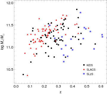
In terms of redshift distribution, our lens candidates are observed in the window , with a median redshift of . This value is larger than the median redshift of SLACS lenses from Auger et al. (2009), i.e. , but consistent within the scatter distribution. Instead, our median redshift is smaller than the average for the SL2S sample from Sonnenfeld et al. (2013), i.e. . This is not surprising given the colour cut of Sect. 2.2. In future analyses this limit will be loosened. The median stellar mass of our sample is with a scatter of dex. The typical uncertainty of the mass estimates is dex too. Within the scatter and mass uncertainties, this value is consistent with the average stellar mass in SLACS (the median is dex and the scatter is dex; Auger et al. 2009) and SL2S lenses (the median is dex and the scatter is ). All the galaxies have , except for KSL669 (see next subsection for further comments about this source). In Fig. 8 we plot the stellar mass as a function of redshift for our sample and the SLACS and SL2S ones.
A similar comparison can be performed for the velocity dispersion, if we consider the KiDS candidates with an available measure of this quantity. The average value for KiDS is 777The velocity dispersions are extracted from both SDSS and BOSS survey, thus, this average value is mixing observations made within two different fibre apertures.. In SLACS, the average is , while in SL2S the velocity dispersion within a radius of one-half effective radius is . The three estimates agree within the scatter distribution and within the typical uncertainties of velocity dispersion measurements of .
4.3.1 A sanity check of the candidates
A sub-sample of candidates has stellar velocity dispersion, , measured in the SDSS (Eisenstein et al., 2011) or BOSS (Dawson et al., 2013) surveys. For these candidates, the knowledge of allows to put constraints on their Einstein radii . For a SIS model, the Einstein radius can be expressed, in radians, as
| (2) |
where , and are, respectively, the angular diameter distances between the observer and the source and between the lens and the source. As a first approximation, in Eq. (2) the strength parameter can be substituted with the measured stellar velocity dispersion, since they have been found to be approximately equal for lens galaxies (see, e.g., Bolton et al. 2008). A more rigorous approach consists of deriving the value of by matching the theoretical velocity dispersion derived from the Jeans equations with the observed one. From the Jeans equations, the radial velocity dispersion can be easily derived. This theoretical quantity is first integrated along the line of sight and then within a circular aperture with SDSS or BOSS fibres radius (i.e., and arcsec, respectively; see Tortora et al. (2009) for equations and further details about the procedure). We use a SIS for the total mass profile, and the light distribution is set adopting a de Vaucouleurs (1948) profile, using the effective radii taken from the SDSS website888http://skyserver.sdss.org/dr13/en/home.aspx which come from a de Vaucoulers fit. Imposing that the theoretical aperture-averaged velocity dispersion is equal to the observed one , the only free parameter, , can be derived. This estimated quantity is finally inserted in Eq. (2).
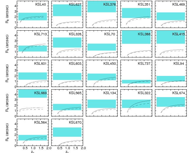
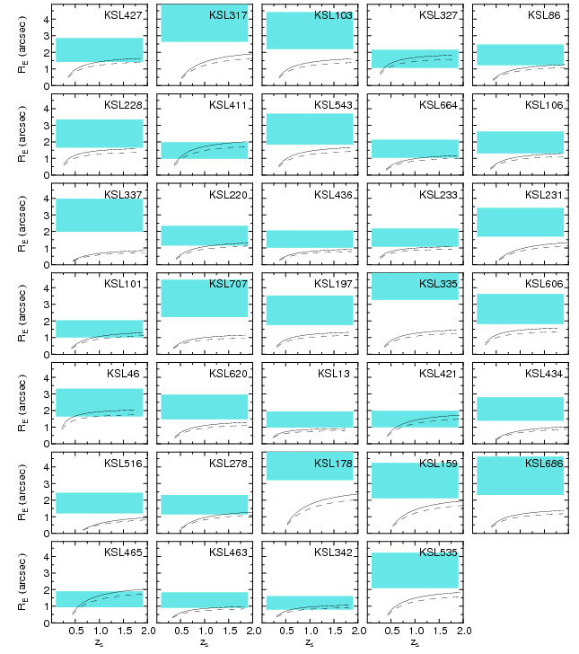
For each lens with a measured , the predicted is plotted as a function of the unknown and compared with the observed Einstein radius (see Fig. 9). A precise determination of the Einstein radius would require modelling of the lensing candidates, which is beyond the scope of this paper, but is planned for a follow-up paper. Here, we simply estimate the Einstein radius visually. We take it to be between 1 and 0.5 times the distance between the arc (or the brightest arc in case of multiple images) and the centre of the lens. This choice is due to the fact that, given a SIS, the image separation for an Einstein ring is exactly twice the Einstein radius, whereas in the case of an arc or an image maximally away from the centre of the lens, the distance from the centre is twice the Einstein radius (Kormann et al., 1994).
In Fig. 9 we show the comparison and we find an overlap for about half of the candidates with measured velocity dispersion. The other half is more likely to be constituted by ring galaxies, foreground sources or other contaminants. An excellent agreement is found for the systems KSL713, KSL450, KSL737, KSL565, KSL322, KSL674 and KSL564. For the other systems, the dynamics predict too small Einstein radii. One interesting case is KSL669, which is a galaxy with a very small stellar mass of . We expect the probability for it to act as a lens to be very small. The comparison performed in Fig. 9 seems to confirm the peculiarity of this lensing candidate. In fact, a larger view of the source shows that it is actually a merger event.
Moreover, among the best ranked systems, KSL627 and KSL376 present a discrepancy which seems difficult to reconcile. These two systems have almost circular blue rings, with and arcsec radii, corresponding to and kpc, respectively. These sources do not match typical Einstein radii observed in galaxy-scale gravitational lenses; they are more likely to belong to the category of ring galaxies (Hoag, 1950; Theys & Spiegel, 1976; Whitmore et al., 1990; Bournaud & Combes, 2003; Iodice et al., 2003; Madore et al., 2009).
ETGs follow a tight relationship between velocity dispersion and stellar mass. This can allow us to predict the velocity dispersion for the remaining galaxies in our final sample. After collecting ETG lenses from SLACS (Auger et al., 2009), we perform a median fit determining the best-fitted relation between the velocity dispersion and the estimated stellar masses. Thus, assuming that this relation holds for our sample and that it has no scatter, we can determine an estimate for the velocity dispersion, when our stellar masses are used. We use Eq. (2) to predict the Einstein radius as a function of the source redshift. The results are shown in Fig. 10, where the dashed line is calculated by inserting the estimated velocity dispersion in Eq. (2), while the solid line is calculated by assuming the average of the ratios obtained for the galaxies with available velocity dispersion, and inserting the derived in Eq. (2). Similar considerations as for the galaxies with measured velocity dispersion can be done for these objects, even if the uncertainties on the estimated velocity dispersions are higher.
The previous analysis can give us an indication on the nature of the candidates. However a spectroscopic validation is needed, because it can not be excluded that the lens candidates are part of a group of galaxies. In this case the stellar velocity dispersion would not trace the dynamics of the group. Indeed, this is the case of the known lens J085446-012137 (KSL317), which is part of a group (Limousin et al., 2010), resulting in a under-estimation of the Einstein radius.
We plan to follow-up our most reliable candidates, mainly for an estimate of the redshift of the arc, in order to confirm or discard their lensing nature.
5 Conclusions
We have developed a new pipeline, based on a Convolutional Neural Network (CNN), to automatically identify strong gravitational lens candidates based mainly on their morphology (Sect. 3). We have applied the method (see Sect. 4) to the third data release of the Kilo Degree Survey (KiDS), which is one of the ESO public surveys carried out with the VLT Survey Telescope (see e.g. de Jong et al., 2015, for a description). Thanks to its high quality images, KiDS is particularly suitable for a search of strong lenses. In the complete survey we expect to find at least 100 LRG lens systems with lens-galaxies at , possibly increasing to several thousand when expanding the search to fainter and higher-redshift galaxies (see Sect. 4.2.1).
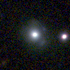
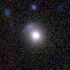
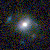
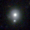
To train the CNN to find lenses, we generated a large sample of simulated lensing features on top of observed colour-magnitude selected galaxies from KiDS (Sect. 3.1.2). The trained network has been applied to a sample of 21789 LRGs in KiDS DR3, retrieving 761 candidates ( of the initial sample). With a visual inspection performed by seven “human” classifiers, we down-selected the most promising 56 lens candidates (Fig. 11). In our starting sample there were three known lenses, two of which were classified correctly as lenses by the CNN and in the subsequent visual inspection phase (Fig. 7). The misclassified lens has an Einstein radius (0.83 arcsec), well below the range where the CNN is trained ( arcsec).
For the candidates with available measures of velocity dispersion or stellar mass estimates, we performed an additional sanity check, suggesting that are solid candidates (Sect. 4.2). Considering the colour-magnitude selection of the lens-galaxy sample, the type of lenses simulated and the completeness, the number is roughly consistent with the expected lenses forecast for the KiDS-DR3 survey area (Sect. 4.2.1). Extending this result to the full KiDS survey, we expect to find LRG lens candidates as a lower limit, similar to the number of lenses in the SLACS sample. Because we limited our search to a very restricted portion of the colour-magnitude and Einstein-radius and magnification space, dominated by luminous lenses and highly magnified sources, the natural next step is to enlarge the colour-magnitude pre-selection of the simulated and observed lenses, which would allow in principle to find up to lenses in the most optimistic scenario (nearly all lenses with signal-to-noise larger than 20 and at least three PSF resolution element for the arc-like images).
A critical aspect to improve in the CNN approach is to reduce the contamination by the false positives which dominate the number of true positives currently by a factor of . This could facilitate, or even eliminate, the need for visual inspection. This factor is consistent with the mis-classifications in the training (see Appendix B), which for the input sample size can lead to false-positive, which is close to the actual number of . Given that the lenses-galaxies are outnumbered by normal galaxies typically by a thousand to one, an important goal is to bring the false-positive rate down to less than 0.1%, without decreasing the true-positive rate substantially. This is a hard task, but human visual inspection suggests that at least 0.25% can be reached (i.e. 56 out of 22 thousand), possibly when including additional colour (RGB) information. Our next goal is to create a completely automated pipeline for lens classification without the need of visual inspection. However, if visual inspection will be needed to down-select lens candidates, it will be important to test the efficiency of the human classifiers in order to be able to estimate accurately the completeness and purity of the final selected sample.
Moreover, for evaluating purity and completeness in a realistic lens search setting, we plan to build a validation-set which reproduces the characteristics of a real survey (where the number of negatives far outnumber the number of positives).
The CNN tends to mis-classify primarily galaxies resembling lensing features (e.g., ring galaxies, mergers, star-forming rings). Thus, training the network on an ensemble of this kind of false-positives would allow the algorithm to learn the subtle differences between the false positives and the true lenses.
The network performance could also be improved with model averaging, i.e., building a series of networks for the same task, but with different structure and parameters, and by averaging their output. Moreover, training the network on galaxy-subtracted images could facilitate the algorithm to pick up more subtle lensing features, especially in the regime of small Einstein radii and bright galaxies. Another possibility is to produce and train the CNN on multi-band images. In this way, colour information would be used to discriminate between lenses with sources and non-lenses.
The final sample of KiDS-DR3 lens candidates suggests that our method is promising to down-selected lens candidates from an input sample by two orders of magnitude. Moreover, it is easily applicable to any ongoing and future survey, (e.g., Euclid, LSST) for classyfing the enormous amount of data that will be produced. In the near future we plan spectroscopic follow-up of our best candidates, to model them, and to better assess their selection biases. In addition, we will apply the method to the full KiDS survey and work on the above-mentioned improvements.


acknowledgements
We thank the anonymous referee for his/her comments that have improved the paper; Sander Dieleman, Davide Punzo, Marco Alexander Wiering, Emmanuel Okafor, Giuseppe Longo, Andrea Colonna and Koen Kuijken for stimulating and useful discussions; Hugo Buddelmeijer, Ewout Helmich and Jelte de Jong for their technical support. LVEK thanks Tom Collett with help in using the code LensPop. CEP, SC, CT, GV, GVK and LVEK are supported through an NWO-VICI grant (project number 639.043.308). GVK acknowledges financial support from the Netherlands Research School for Astronomy (NOVA) and Target. Target is supported by Samenwerkingsverband Noord Nederland, European fund for regional development, Dutch Ministry of economic affairs, Pieken in de Delta, Provinces of Groningen and Drenthe. PS is supported by the Deutsche Forschungsgemeinschaft in the framework of the TR33 ‘The Dark Universe’.
References
- Alard (2006) Alard C., 2006, preprint, (arXiv:astro-ph/0606757)
- Arnouts et al. (1999) Arnouts S., Cristiani S., Moscardini L., Matarrese S., Lucchin F., Fontana A., Giallongo E., 1999, MNRAS, 310, 540
- Auger et al. (2009) Auger M. W., Treu T., Bolton A. S., Gavazzi R., Koopmans L. V. E., Marshall P. J., Bundy K., Moustakas L. A., 2009, ApJ, 705, 1099
- Barnabè et al. (2009) Barnabè M., Czoske O., Koopmans L. V. E., Treu T., Bolton A. S., Gavazzi R., 2009, MNRAS, 399, 21
- Barnabè et al. (2011) Barnabè M., Czoske O., Koopmans L. V. E., Treu T., Bolton A. S., 2011, MNRAS, 415, 2215
- Benítez (2000) Benítez N., 2000, ApJ, 536, 571
- Bertin & Arnouts (1996) Bertin E., Arnouts S., 1996, A&AS, 117, 393
- Binney & Merrifield (1998) Binney J., Merrifield M., 1998, Galactic Astronomy. Princeton University Press
- Bolton et al. (2008) Bolton A. S., Burles S., Koopmans L. V. E., Treu T., Gavazzi R., Moustakas L. A., Wayth R., Schlegel D. J., 2008, ApJ, 682, 964
- Bom et al. (2016) Bom C. R., Makler M., Albuquerque M. P., Brandt C. H., 2016, preprint, (arXiv:1607.04644)
- Bonvin et al. (2016) Bonvin V., et al., 2016, preprint, (arXiv:1607.01790)
- Boureau et al. (2010) Boureau Y.-L., Bach F., LeCun Y., Ponce J., 2010, in Computer Vision and Pattern Recognition (CVPR), 2010 IEEE Conference on. pp 2559–2566
- Bournaud & Combes (2003) Bournaud F., Combes F., 2003, A&A, 401, 817
- Brault & Gavazzi (2015) Brault F., Gavazzi R., 2015, A&A, 577, A85
- Brewer et al. (2012) Brewer B. J., et al., 2012, MNRAS, 422, 3574
- Bruzual & Charlot (2003) Bruzual G., Charlot S., 2003, MNRAS, 344, 1000
- Cao et al. (2016) Cao S., Biesiada M., Yao M., Zhu Z.-H., 2016, MNRAS, 461, 2192
- Capaccioli & Schipani (2011) Capaccioli M., Schipani P., 2011, The Messenger, 146, 2
- Cardone & Tortora (2010) Cardone V. F., Tortora C., 2010, MNRAS, 409, 1570
- Cardone et al. (2009) Cardone V. F., Tortora C., Molinaro R., Salzano V., 2009, A&A, 504, 769
- Carlstrom et al. (2011) Carlstrom J. E., et al., 2011, PASP, 123, 568
- Chabrier (2001) Chabrier G., 2001, ApJ, 554, 1274
- Chae (2003) Chae K.-H., 2003, MNRAS, 346, 746
- Chevance et al. (2012) Chevance M., Weijmans A.-M., Damjanov I., Abraham R. G., Simard L., van den Bergh S., Caris E., Glazebrook K., 2012, ApJ, 754, L24
- Colless et al. (2001) Colless M., et al., 2001, MNRAS, 328, 1039
- Collett (2015) Collett T. E., 2015, ApJ, 811, 20
- Dawson et al. (2013) Dawson K. S., et al., 2013, AJ, 145, 10
- Deane et al. (2013) Deane R. P., Rawlings S., Garrett M. A., Heywood I., Jarvis M. J., Klöckner H.-R., Marshall P. J., McKean J. P., 2013, MNRAS, 434, 3322
- Dieleman et al. (2015) Dieleman S., Willett K. W., Dambre J., 2015, MNRAS, 450, 1441
- Eisenstein et al. (2001) Eisenstein D. J., et al., 2001, AJ, 122, 2267
- Eisenstein et al. (2011) Eisenstein D. J., et al., 2011, AJ, 142, 72
- Estrada et al. (2007) Estrada J., et al., 2007, ApJ, 660, 1176
- Ferreras et al. (2010) Ferreras I., Saha P., Leier D., Courbin F., Falco E. E., 2010, MNRAS, 409, L30
- Foëx et al. (2013) Foëx G., Motta V., Limousin M., Verdugo T., More A., Cabanac R., Gavazzi R., Muñoz R. P., 2013, A&A, 559, A105
- Fukugita et al. (1992) Fukugita M., Futamase T., Kasai M., Turner E., 1992, ApJ, 393, 3
- Fukushima (1980) Fukushima K., 1980, Biological cybernetics, 36, 193
- Gavazzi et al. (2007) Gavazzi R., Treu T., Rhodes J. D., Koopmans L. V. E., Bolton A. S., Burles S., Massey R. J., Moustakas L. A., 2007, ApJ, 667, 176
- Gavazzi et al. (2014) Gavazzi R., Marshall P. J., Treu T., Sonnenfeld A., 2014, ApJ, 785, 144
- Grillo et al. (2010) Grillo C., Eichner T., Seitz S., Bender R., Lombardi M., Gobat R., Bauer A., 2010, ApJ, 710, 372
- Grogin et al. (2011) Grogin N. A., et al., 2011, ApJS, 197, 35
- Guo et al. (2016) Guo Y., Liu Y., Oerlemans A., Lao S., Wu S., Lew M. S., 2016, Neurocomputing, 187, 27
- Hála (2014) Hála P., 2014, preprint, (arXiv:1412.8341)
- He et al. (2015a) He K., Zhang X., Ren S., Sun J., 2015a, in Proceedings of the IEEE International Conference on Computer Vision. pp 1026–1034
- He et al. (2015b) He K., Zhang X., Ren S., Sun J., 2015b, CoRR, abs/1512.03385
- Hinton et al. (2012) Hinton G. E., Srivastava N., Krizhevsky A., Sutskever I., Salakhutdinov R. R., 2012, preprint, (arXiv:1207.0580)
- Hoag (1950) Hoag A. A., 1950, AJ, 55, 170
- Horesh et al. (2005) Horesh A., Ofek E. O., Maoz D., Bartelmann M., Meneghetti M., Rix H.-W., 2005, ApJ, 633, 768
- Hoyle (2016) Hoyle B., 2016, Astronomy and Computing, 16, 34
- Huertas-Company et al. (2015) Huertas-Company M., et al., 2015, ApJS, 221, 8
- Ilbert et al. (2006) Ilbert O., et al., 2006, A&A, 457, 841
- Impellizzeri et al. (2008) Impellizzeri C. M. V., McKean J. P., Castangia P., Roy A. L., Henkel C., Brunthaler A., Wucknitz O., 2008, Nature, 456, 927
- Iodice et al. (2003) Iodice E., Arnaboldi M., Bournaud F., Combes F., Sparke L. S., van Driel W., Capaccioli M., 2003, ApJ, 585, 730
- Ioffe & Szegedy (2015) Ioffe S., Szegedy C., 2015, preprint, (arXiv:1502.03167)
- Jiang & Kochanek (2007) Jiang G., Kochanek C. S., 2007, ApJ, 671, 1568
- Joseph et al. (2014) Joseph R., et al., 2014, A&A, 566, A63
- Kim & Brunner (2016) Kim E. J., Brunner R. J., 2016, preprint, (arXiv:1608.04369)
- Kingma & Ba (2014) Kingma D., Ba J., 2014, preprint, (arXiv:1412.6980)
- Kochanek (1996) Kochanek C., 1996, ApJ, 473, 595
- Koopmans & Treu (2003) Koopmans L. V. E., Treu T., 2003, ApJ, 583, 606
- Koopmans et al. (2006) Koopmans L. V. E., Treu T., Bolton A. S., Burles S., Moustakas L. A., 2006, ApJ, 649, 599
- Koopmans et al. (2009) Koopmans L. V. E., et al., 2009, ApJ, 703, L51
- Kormann et al. (1994) Kormann R., Schneider P., Bartelmann M., 1994, A&A, 284, 285
- Kubo & Dell’Antonio (2008) Kubo J. M., Dell’Antonio I. P., 2008, MNRAS, 385, 918
- Kuijken (2011) Kuijken K., 2011, The Messenger, 146, 8
- LSST Science Collaboration et al. (2009) LSST Science Collaboration et al., 2009, preprint, (arXiv:0912.0201)
- Laureijs et al. (2011) Laureijs R., et al., 2011, arXiv.org
- LeCun et al. (1998) LeCun Y., Bottou L., Bengio Y., Haffner P., 1998, Proceedings of the IEEE, 86, 2278
- LeCun et al. (2015) LeCun Y., Bengio Y., Hinton G., 2015, Nature, 521, 436
- Leier et al. (2016) Leier D., Ferreras I., Saha P., Charlot S., Bruzual G., La Barbera F., 2016, MNRAS, 459, 3677
- Lenzen et al. (2004) Lenzen F., Schindler S., Scherzer O., 2004, A&A, 416, 391
- Li et al. (2016) Li R., Frenk C. S., Cole S., Gao L., Bose S., Hellwing W. A., 2016, MNRAS, 460, 363
- Limousin et al. (2010) Limousin M., et al., 2010, A&A, 524, A95
- Liske et al. (2015) Liske J., et al., 2015, MNRAS, 452, 2087
- Madore et al. (2009) Madore B. F., Nelson E., Petrillo K., 2009, ApJS, 181, 572
- Marshall et al. (2016) Marshall P. J., et al., 2016, MNRAS, 455, 1171
- Mason et al. (2016) Mason C. A., et al., 2016, preprint, (arXiv:1610.03075)
- Maturi et al. (2014) Maturi M., Mizera S., Seidel G., 2014, A&A, 567, A111
- McKean et al. (2015) McKean J., et al., 2015, Proceedings of Science, p. 84
- Miyazaki et al. (2012) Miyazaki S., et al., 2012, in SPIE Astronomical Telescopes+ Instrumentation. pp 84460Z–84460Z
- Möller et al. (2007) Möller O., Kitzbichler M., Natarajan P., 2007, MNRAS, 379, 1195
- More et al. (2008) More A., McKean J. P., Muxlow T. W. B., Porcas R. W., Fassnacht C. D., Koopmans L. V. E., 2008, MNRAS, 384, 1701
- More et al. (2011) More A., Jahnke K., More S., Gallazzi A., Bell E. F., Barden M., Häußler B., 2011, ApJ, 734, 69
- More et al. (2012) More A., Cabanac R., More S., Alard C., Limousin M., Kneib J.-P., Gavazzi R., Motta V., 2012, ApJ, 749, 38
- More et al. (2016) More A., et al., 2016, MNRAS, 455, 1191
- Nair & Hinton (2010) Nair V., Hinton G. E., 2010, in Proceedings of the 27th International Conference on Machine Learning (ICML-10). pp 807–814
- Negrello et al. (2010) Negrello M., et al., 2010, Science, 330, 800
- Ng (2004) Ng A. Y., 2004, in Proceedings of the twenty-first international conference on Machine learning. p. 78
- Oguri (2006) Oguri M., 2006, MNRAS, 367, 1241
- Oguri & Marshall (2010) Oguri M., Marshall P. J., 2010, MNRAS, 405, 2579
- Pawase et al. (2012) Pawase R. S., Faure C., Courbin F., Kokotanekova R., Meylan G., 2012, preprint, (arXiv:1206.3412)
- Posacki et al. (2015) Posacki S., Cappellari M., Treu T., Pellegrini S., Ciotti L., 2015, MNRAS, 446, 493
- Richard et al. (2011) Richard J., Kneib J.-P., Ebeling H., Stark D. P., Egami E., Fiedler A. K., 2011, MNRAS, 414, L31
- Ruff et al. (2011) Ruff A. J., Gavazzi R., Marshall P. J., Treu T., Auger M. W., Brault F., 2011, ApJ, 727, 96
- Rumelhart et al. (1986) Rumelhart D. E., Hinton G. E., Williams R. J., 1986, Nature, 323, 533
- Russakovsky et al. (2015) Russakovsky O., et al., 2015, International Journal of Computer Vision (IJCV), 115, 211
- Schlafly & Finkbeiner (2011) Schlafly E. F., Finkbeiner D. P., 2011, ApJ, 737, 103
- Schlegel et al. (1998) Schlegel D. J., Finkbeiner D. P., Davis M., 1998, ApJ, 500, 525
- Schmidhuber (2015) Schmidhuber J., 2015, Neural Networks, 61, 85
- Schneider et al. (1992) Schneider P., Ehlers J., Falco E., 1992, Gravitational Lenses. Springer-Verlag Berlin Heidelberg New York. Also Astronomy and Astrophysics Library
- Seidel & Bartelmann (2007) Seidel G., Bartelmann M., 2007, A&A, 472, 341
- Sersic (1968) Sersic J. L., 1968, Atlas de galaxias australes
- Simard et al. (2003) Simard P. Y., Steinkraus D., Platt J. C., 2003, in Proceedings of the Seventh International Conference on Document Analysis and Recognition - Volume 2. ICDAR ’03. IEEE Computer Society, Washington, DC, USA, pp 958–, http://dl.acm.org/citation.cfm?id=938980.939477
- Sonnenfeld et al. (2013) Sonnenfeld A., Treu T., Gavazzi R., Suyu S. H., Marshall P. J., Auger M. W., Nipoti C., 2013, ApJ, 777, 98
- Sonnenfeld et al. (2015) Sonnenfeld A., Treu T., Marshall P. J., Suyu S. H., Gavazzi R., Auger M. W., Nipoti C., 2015, ApJ, 800, 94
- Spiniello et al. (2011) Spiniello C., Koopmans L., Trager S. C., Czoske O., Treu T., 2011, 417, 3000
- Suyu et al. (2010) Suyu S. H., Marshall P. J., Auger M. W., Hilbert S., Blandford R. D., Koopmans L. V. E., Fassnacht C. D., Treu T., 2010, ApJ, 711, 201
- Swinbank et al. (2009) Swinbank A. M., et al., 2009, MNRAS, 400, 1121
- The Dark Energy Survey Collaboration (2005) The Dark Energy Survey Collaboration 2005, preprint, (arXiv:astro-ph/0510346)
- Theano Development Team (2016) Theano Development Team 2016, arXiv e-prints, abs/1605.02688
- Theys & Spiegel (1976) Theys J. C., Spiegel E. A., 1976, ApJ, 208, 650
- Tortora et al. (2009) Tortora C., Napolitano N. R., Romanowsky A. J., Capaccioli M., Covone G., 2009, MNRAS, 396, 1132
- Tortora et al. (2010) Tortora C., Napolitano N., Romanowsky A., Jetzer P., 2010, ApJ, 721, L1
- Treu & Koopmans (2002a) Treu T., Koopmans L. V. E., 2002a, MNRAS, 337, L6
- Treu & Koopmans (2002b) Treu T., Koopmans L. V. E., 2002b, ApJ, 575, 87
- Treu et al. (2010) Treu T., Auger M. W., Koopmans L. V. E., Gavazzi R., Marshall P. J., Bolton A. S., 2010, ApJ, 709, 1195
- Treu et al. (2015) Treu T., et al., 2015, ApJ, 812, 114
- Trujillo et al. (2007) Trujillo I., Conselice C. J., Bundy K., Cooper M. C., Eisenhardt P., Ellis R. S., 2007, MNRAS, 382, 109
- Turner et al. (1984) Turner E. L., Ostriker J. P., Gott III J. R., 1984, ApJ, 284, 1
- Valentijn et al. (2007) Valentijn E. A., et al., 2007, in Shaw R. A., Hill F., Bell D. J., eds, Astronomical Society of the Pacific Conference Series Vol. 376, Astronomical Data Analysis Software and Systems XVI. p. 491 (arXiv:astro-ph/0702189)
- Van der Walt et al. (2014) Van der Walt S., Schönberger J. L., Nunez-Iglesias J., Boulogne F., Warner J. D., Yager N., Gouillart E., Yu T., 2014, PeerJ, 2, e453
- Vegetti & Koopmans (2009) Vegetti S., Koopmans L. V. E., 2009, MNRAS, 400, 1583
- Verdugo et al. (2014) Verdugo T., et al., 2014, A&A, 571, A65
- Whitmore et al. (1990) Whitmore B. C., Lucas R. A., McElroy D. B., Steiman-Cameron T. Y., Sackett P. D., Olling R. P., 1990, AJ, 100, 1489
- de Jong et al. (2015) de Jong J. T. A., et al., 2015, A&A, 582, A62
- de Jong et al. (2017) de Jong J. T. A., et al., 2017, preprint, (arXiv:1703.02991)
- de Vaucouleurs (1948) de Vaucouleurs G., 1948, Annales d’Astrophysique, 11, 247
Appendix A Neural Networks
In this appendix we give a short introduction on the theory of Convolutional Neural Networks (CNN).
A.1 Feed-forward neural network
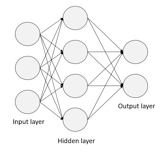
A feed-forward neural network, as the one shown schematically in Fig. 14, is a basic example of a deep-learning algorithm that can be schematized as an ensemble of connected units. The input layer is the representation of a single element of the training set, where the units are the components of the data-point vector . Every unit in the hidden layer performs the following transformation of its inputs
| (3) |
where the vector is called the weight vector and the constant is the bias. The non-linear activation function, is often the Rectified linear unit (ReLU; Nair & Hinton 2010)
| (4) |
or the sigmoid function
| (5) |
Hidden layers are stacked sequentially until the topmost, i.e. the output layer, is reached. We want the output layer to approximate the desired output . This is obtained by finding the weights and biases that minimize a chosen loss function . The minimization is most often done via the iterative process of gradient descent. For each layer the weights and biases are updated in the following way
| (6) |
where is a constant called the learning rate. The gradients are computed via the back-propagation algorithm (Rumelhart et al., 1986).
A.2 Convolutional Neural Network
In Convolutional Neural Networks, the input data has a topological structure (e.g. an image) and is not presented as a vector but as a set of matrices with (e.g., the R, G and B components of an image. In this case ). The main component of a CNN is the convolutional layer, which takes the inputs and, through a set of filters, produces a stack of feature maps with equal to the number of filters. Every filter (also called kernel) in the convolutional layer produces a feature map through a convolution
| (7) |
where is the convolution operator, is a non linear function as in eq. (3), are the weight matrices with , representing a filter with its bias given by the constant matrix . There are far fewer parameters to be determined in a convolutional layer as compared to a fully connected layer because, practically, we are replacing the dot product of Eq. (3) with a convolution, and, in all the practical cases, the weight matrices have spatial dimensions much smaller than the input dimension (usually 3 by 3).
Convolutional layers are sequentially stacked such as the input of the deeper layers are the feature maps. In between then there are non-linear and other transformations (e.g. pooling). After the training is complete, in each layer we have a representation of the input data of increasing complexity (i.e. the different feature maps) each produced by a different filter which represents a particular feature learned during the training phase. The output layer of a CNN is the same as in a feed-forward neural network and can be preceded by one or more hidden fully-connected layers. Its function is to classify the last layer of feature maps created by the CNN, giving as output one ore more numbers which represent the outcome of the classification.

| Type | Filters/Units | Filter size | Padding | Non-linearity | Initial weights | Initial biases |
|---|---|---|---|---|---|---|
| Convolutional | 32 | 3 | ReLU | HeNormal | 0 | |
| Max-pooling | - | - | - | - | - | |
| Convolutional | 64 | 1 | ReLU | HeNormal | 0 | |
| Max-pooling | - | - | - | - | - | |
| Convolutional | 128 | 1 | ReLU | HeNormal | 0 | |
| Convolutional | 128 | 1 | ReLU | HeNormal | 0 | |
| Fully connected | 1024 | - | - | ReLU | HeNormal | 0 |
| Fully connected | 1024 | - | - | ReLU | HeNormal | 0 |
| Max-pooling | - | 1 | - | - | - | - |
| Fully connected | 1 | 2 | - | sigmoid | HeNormal | 0 |
Appendix B CNN implementation
Our CNN is implemented in Python 2.7 using the open-source libraries Lasagne999http://github.com/Lasagne/Lasagne/ and Theano101010http://deeplearning.net/software/theano/ (Theano Development Team, 2016). The training of the CNN is executed on a GeForce GTX 760 in parallel with the data augmentation performed on the CPU using the scikit-image111111http://scikit-image.org/ package (Van der Walt et al., 2014). The training time with this configuration takes about 2 hours. While the CNN takes about 20 minutes to classify the LRG sample. In this Appendix we provide the technical details of the implementation and training of our CNN (Sections B.1 and B.2).
B.1 Network architecture
In Fig. 15 and in Table 3 we show the architecture of our CNN. ReLU (see Eq. (5)) is applied after each convolutional and fully connected layer. The 60 by 60 input layer is followed by four convolutional layers with 32, 64, 128 and 128 filters, respectively. All the filters have 3 by 3 sizes except for the first convolutional layer which has a filter size of 7 by 7. In the convolutional kernels we use untied bias. To preserve the input volume through the convolution and not degrade the information at the borders of the input, we zero-pad the input of the convolutional layers with 3, 1, 1 and 1 pixels respectively. Max-pooling (Boureau et al., 2010) with a kernel size of 2 by 2 is used after the first and the second convolutional layer and after the second fully-connected layer with a 1D kernel size of 2. Max-pooling takes the maximum value in a connected set of elements of the feature maps. There are two main consequences of using Max-pooling: a) reducing the dimensionality of the data and the parameters to be estimated, b) teaching translational invariance to the network, because slightly shifted inputs will produce the same feature maps. Two fully-connected layers of 1024 units follow the set of convolutional and max-pooling layers. Finally, we use a sigmoid non-linear output unit which gives a real number between 0 and 1 that represents the probability of being a strong gravitational lensing system. We use batch normalization (Ioffe & Szegedy, 2015) before the non-linearity of each layer. A batch normalization layer operates on the inputs of the non-linearities normalizing the data in order to have zero mean and unit variance among the mini-batch. Then, the data is fed to a linear function with two learnable parameters that has the property to revert or modify the normalization. The chosen architecture implies that our network has about 30 million of trainable parameters.
B.2 Training
The network is trained by minimizing a loss function of the targets (1 for lenses and 0 for non-lenses) and the predictions (the output of the sigmoid unit of network). We use the binary cross-entropy, a common choice in two-class classification problems:
| (8) |
The minimization is done via mini-batch stochastic gradient descent with ADAM updates (Kingma & Ba, 2014). The advantage of using ADAM updates is the introduction of a friction term that mitigates the gradient momentum in order to reach a faster convergence. In addition, the updates have a per-parameter adaptation, i.e., they have a different effective learning rate for the different parameters depending on the gradient values. We used a batch size of 600 images and perform 10000 gradient updates, which corresponds to six million examples. Each mini-batch is composed by 300 lens and 300 non-lens examples. After an initial exploration, we start with a learning rate of 0.004, decrease it to 0.0004 after three million training examples and to 0.00004 after 5.5 million training examples (the choice of the values for the learning rate has been fundamental for training successfully the network). The weights of each filter are initialized, as discussed in He et al. (2015a), from a random normal distribution with variance where is the number of inputs of the unit. The initial values of the biases are set to zero. We use dropout (Hinton et al., 2012) in the fully connected layers. Dropout consists of switching off units randomly during each update of the training phase. This has two main consequences: a) a speed-up of the training phase, because of the reduced number of parameters to be computed in the fully connected-layers of the CNN, b) reducing the possibility of over-fitting, since the network tends to learn features that better generalize the data. We also use L2-norm regularization (see e.g., Ng 2004) with . The regularization adds to the loss function Eq. (8) another factor given by the squared sum of all the weights times the factor . It has the property to let the network prefer to learn small diffuse weights penalizing the creation of peaky ones. In this way a classification, based on all the data coming from the input, tends to be promoted over one where the weights tend to consider only a subset of the input.
B.3 Analysis
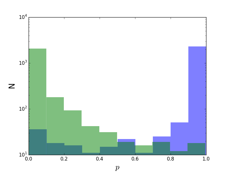
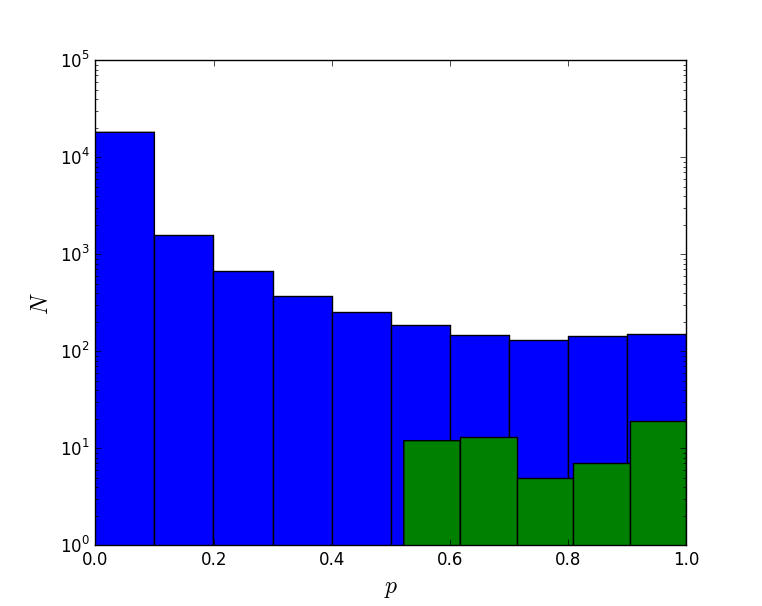
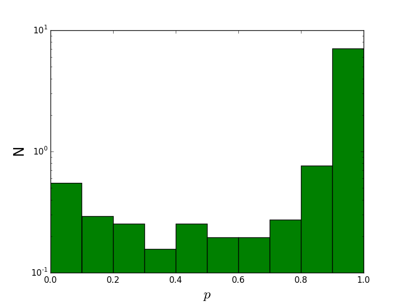
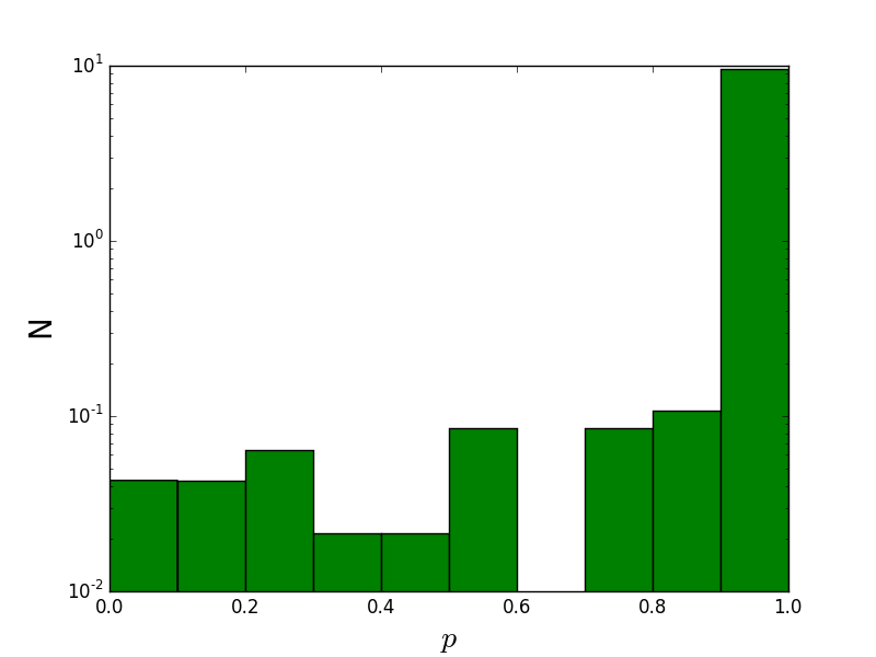
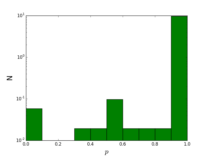
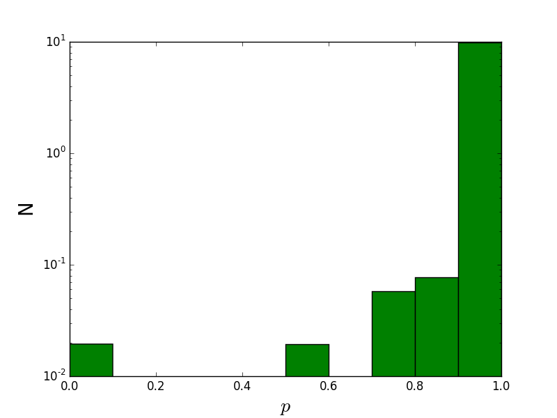
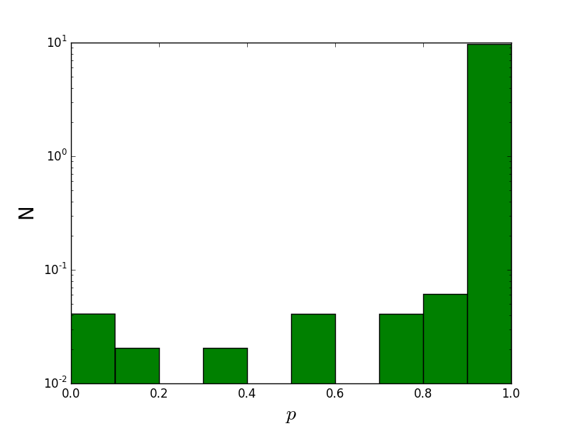
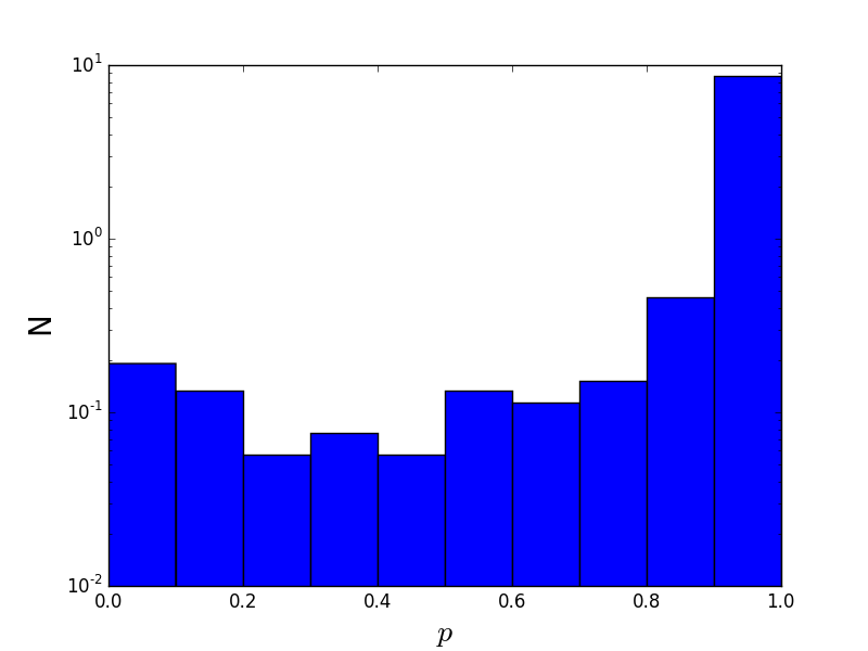
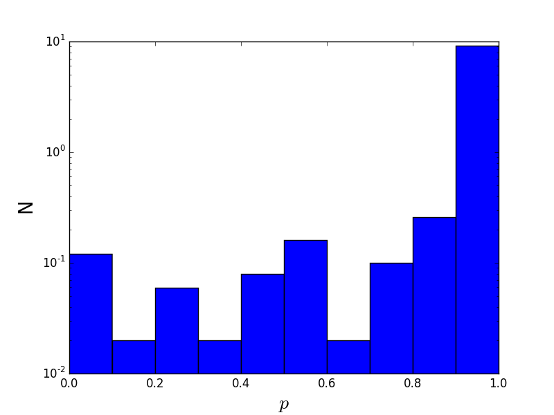
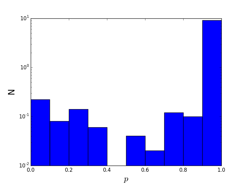
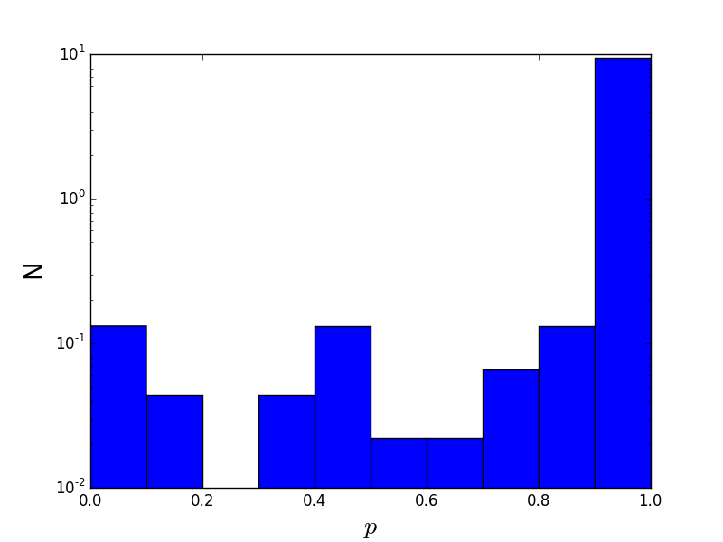
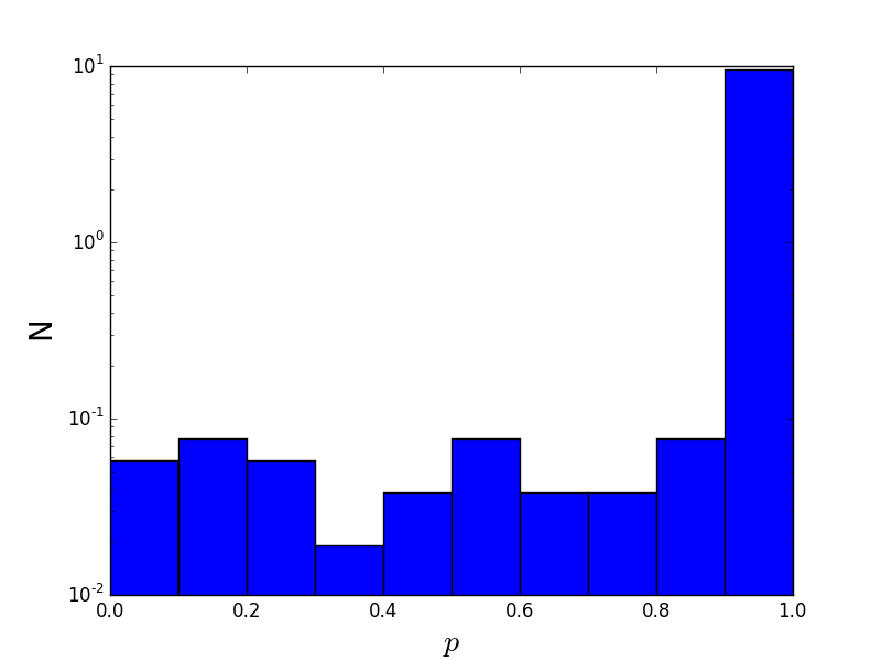
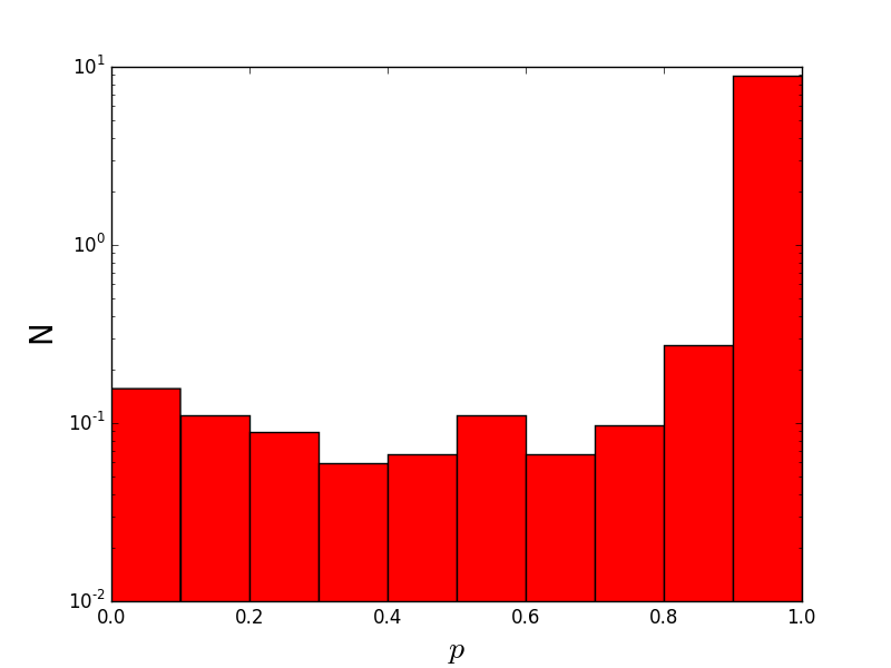
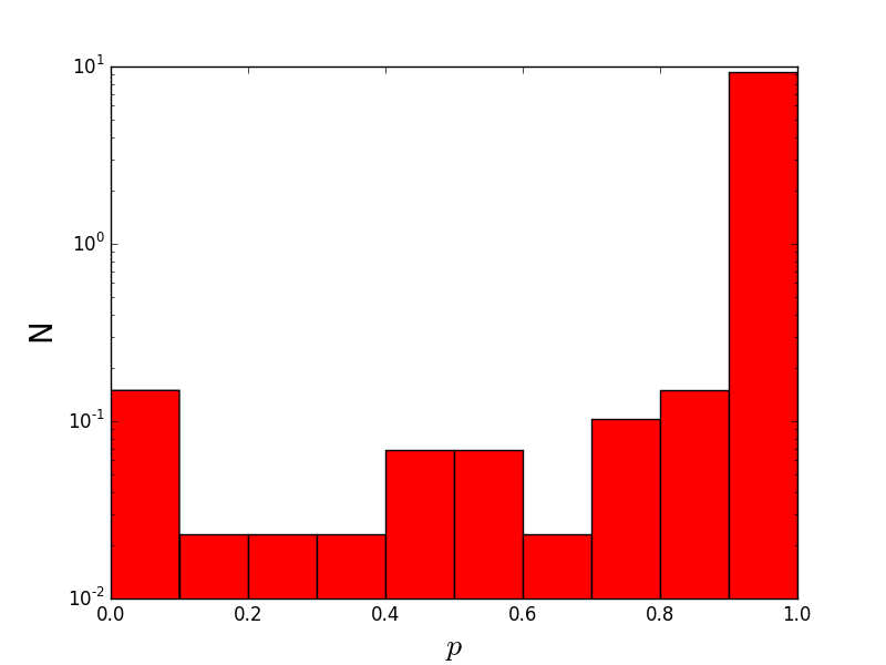
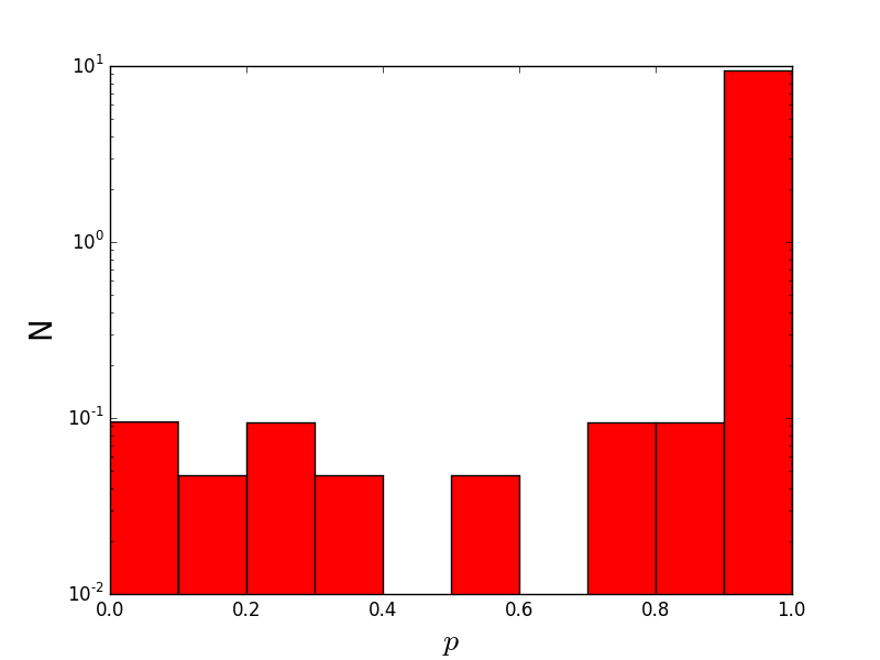
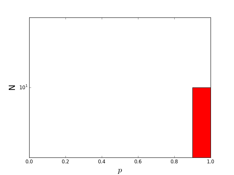
For monitoring the network during the training we build a fixed validation set composed of 5000 images (half lenses, half non-lenses) with the same prescriptions as summarized in Sect. 3.2. At the end of the training the network reaches a 96% accuracy for both the lens and non-lens examples. Fig. 16 shows the distribution of the network output for the validation set. For values of greater than 0.5 the lens examples start to be dominant in the distribution. To check if there is any correlation between and the characteristics of the simulated mock sources, we investigate the distribution of the lens examples for different ranges of three parameters: Einstein radii, magnification and ratio between the peak brightness of the source and the lens. From Fig. 18 one can see that the distributions are skewed to higher values for the higher ranges of the parameters considered (larger, brighter and more magnified lens systems). This implies that the classification is more accurate for the training examples with higher magnification, higher Einstein radius and more luminous sources with respect to the KiDS galaxy. In Fig. 17 we show the distribution of the network output of -values for the full LRG sample and the 56 lens candidates (a sub-sample of the 761 candidates with ) . We do not retrieve a significant peaked distribution in the far end as for the validation set. This could be due to the intrinsic difference between real and simulated data. In addition, we have far fewer lenses in the LRG sample compared to the non-lenses. Moreover, the lenses in the validation set are uniformly distributed in the range of the parameters of Table 1. Thus, for a proper comparison, a validation set that reproduces the numbers and the distribution of the parameters for real lenses should be created.

Appendix C r-band images of the candidates
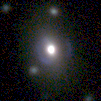
In Fig. 19 we show the r-band images of the 56 candidates selected through the visual inspection of Sect. 4.1. r-band KiDS images have been used as the actual input of the CNN with the purpose of finding lens candidates.
