©2017 International World Wide Web Conference Committee
(IW3C2), published under Creative Commons CC BY 4.0 License.
Competition and Selection Among Conventions
Cascades: A View from Audience
Abstract
Cascades on social and information networks have been a tremendously popular subject of study in the past decade, and there is a considerable literature on phenomena such as diffusion mechanisms, virality, cascade prediction, and peer network effects. Against the backdrop of this research, a basic question has received comparatively little attention: how desirable are cascades on a social media platform from the point of view of users? While versions of this question have been considered from the perspective of the producers of cascades, any answer to this question must also take into account the effect of cascades on their audience — the viewers of the cascade who do not directly participate in generating the content that launched it. In this work, we seek to fill this gap by providing a consumer perspective of information cascades.
Users on social and information networks play the dual role of producers and consumers, and our work focuses on how users perceive cascades as consumers. Starting from this perspective, we perform an empirical study of the interaction of Twitter users with retweet cascades. We measure how often users observe retweets in their home timeline, and observe a phenomenon that we term the Impressions Paradox: the share of impressions for cascades of size decays much more slowly than frequency of cascades of size . Thus, the audience for cascades can be quite large even for rare large cascades. We also measure audience engagement with retweet cascades in comparison to non-retweeted or organic content. Our results show that cascades often rival or exceed organic content in engagement received per impression. This result is perhaps surprising in that consumers didn’t opt in to see tweets from these authors. Furthermore, although cascading content is widely popular, one would expect it to eventually reach parts of the audience that may not be interested in the content. Motivated by the tension in these empirical findings, we posit a simple theoretical model that focuses on the effect of cascades on the audience (rather than the cascade producers). Our results on this model highlight the balance between retweeting as a high-quality content selection mechanism and the role of network users in filtering irrelevant content. In particular, the results suggest that together these two effects enable the audience to consume a high quality stream of content in the presence of cascades.
keywords:
Cascade Models; Consumer; Twitter1 Introduction
Users on modern social and information networks play dual roles as content producers and consumers: content they produce is seen by their friends or followers, and content they see (or consume) on the network is produced by users they are friends with or following. In addition to producing their own content, these networks also provide users with low-friction content-producing mechanisms. Users can switch from being consumers to content producers with a single click as they can share or retweet content that they want to communicate to their followers. In some cases, just consumption activity (such as “liking”) is akin to content production from the user in terms of what their followers/friends observe.
Having a low barrier for content production is clearly important in activating the information-sharing aspects of social and information networks, but some of these mechanisms could be viewed as existing in tension with a basic contract of these networks. A key premise of a social or information network is that users opt in to connect to friends or users that they are explicitly interested in hearing from. But in the presence of sharing mechanisms, cascades originate on the network and hence a user could often see content from users they did not opt in to see content from. It is conceivable that cascades could overwhelm a user’s home timeline, rendering the network significantly less useful to the user. Indeed, when retweets were first introduced on Twitter, users expressed many such concerns [4].
A key question then is: what effect do cascades have on consumption behavior? A pithy answer is provided by the existence of networks with hundreds of millions of active users; this at least suggests that the effect of cascades is not as negative as users feared it to be. Our work aims to quantify this effect, and provide some insight into why this might be the case.
One aspect of user consumption behavior is deeply intertwined with production in that production of content (via re-sharing) is also simultaneously consumption behavior. Production has been widely studied in the literature under the topics of information propagation and diffusion of content. We note however that this is only a part of consumption and some basic characteristics of consumption behavior have not been addressed to the best of our knowledge. For instance, although virality of content on Twitter has been extensively discussed [13, 23], we do not understand the view of virality from a consumer perspective: what fraction of tweets consumed by consumers on Twitter are viral? Do users engage with these more than with non-viral content in their home timeline? We emphasize that the consumer view could be quite different from the producer perspective for virality: even though a small fraction of tweets “go viral”, a large fraction of the consumer experience on Twitter could still be shaped by viral content. This is because when we think about the population of all views of tweets, we’re sampling tweets in proportion to their popularity, and this sampling based on size leads to effects where a small number of items (extremely popular tweets in this case) can make up a large fraction of the sample [2].
We examine the above questions through empirical analysis of user behavior on Twitter. Each time a user views a tweet — referred to as an impression of the tweet — they can choose to engage with it through several means, including clicking on it, liking it, or retweeting it. Given observations of what tweets a user sees in their home timeline via tweet impression logs, as well as tweet engagement and sharing activity, we can piece together a consumer view of cascades on Twitter. Through this analysis, we observe that retweet cascades indeed occupy a substantial fraction (roughly a quarter) of a typical user’s timeline, and 1 out of 3 impressions in the dataset we analyze are due to cascades. Thus, cascades have a substantial impact on the user experience at Twitter given their prevalence in users’ home timelines. This impact is arising despite the fact that extremely few tweets generate large cascades; the point is that for a producer of content, it is very rare to see your tweet become viral, but for a consumer of content, much of your time is spent looking at viral content. We term this dichotomy the Impressions Paradox; it is a counter-intuitive contrast in two ways of looking at the same population, in the spirit of similar phenomena that arise because of sampling biased by size.
In light of our previous discussion, we note that this wide prevalence of retweets does indeed impose upon users content that they did not opt in to see. It is natural to wonder whether users respond negatively to this imposition on their home timeline, which they have carefully constructed through their choice of users to follow.
Analyzing user engagement with cascades provides a way to answer this question. In particular, we compare user engagement probabilities (retweeting, liking and clicking) on retweeted content versus organic content (directly produced by a person the user follows). Our main finding here is that retweeted content rivals or exceeds the organic content in engagement. It is useful to consider this fact in the context of user fears of irrelevant content showing up in their timeline (even if it might be high quality; the best tweet on politics may be uninteresting to a user not interested in politics). Viewed in this light, our finding is perhaps quite unexpected. On the other hand, this result is exactly what one might expect if we think of retweets as a high quality tweet selection mechanism — users might only engage with the best tweets, so it is unsurprising that the best tweets get high engagement. Note however, that popular tweets also get viewed by many users, resulting in a very high number of impressions. Thus, even with an assumption that popular tweets have high quality, it seems unclear why they should get high engagement per impression as their growth in audience size might completely outpace the set of interested users.
In order to understand this effect quantitatively, we propose and analyze a simple theoretical model of retweeting behavior that teases apart these two effects. Our model is novel in that it inverts the traditional view of cascades as a tree being rooted at the author, to a tree that is centered at an arbitrary user — a member of the audience for cascades — who receives a mix of organic tweets and retweets. This model helps us quantify two metrics for a user’s home timeline: precision (seeing content that is relevant or topical for users) and quality (highly engaging content for a topic). Intuitively, users would like to have a high precision and high quality home timeline where most of the content is relevant and highly engaging. In the presence of retweets, it seems unclear a priori whether the content will still be relevant, and further how would one quantify changes in tweet quality. Our analytical and simulation results show that it is indeed possible for users to have the best of both worlds by seeing high quality and relevant retweets in their timeline. Furthermore, this model also helps us understand the value of retweets by quantifying a counterfactual world where retweets would not exist.
2 Related work
There has been extensive work on on-line information diffusion. This has included studies of news [1, 5, 3], recommendations [14], quotes [8], hashtags on Twitter [18, 21, 19, 15, 16], information flow on Twitter [23] and memes on Facebook [9, 7]. Past work has also investigated methodological issues including definitions of virality [12], the problem of prediction [7], the trade-off between precision and recall in cascading content [6], and the role of mathematical epidemic models [11].
In addition, it has been shown that only a very small fraction of cascades become viral [12] but the ones that do become viral cover a large/diverse set of users. In other words, if you are the source of a cascade you have a low chance of creating a viral cascade but, once we switch to the consumer’s point of view we observe that a large fraction of a user’s timeline is made up of these diffusing pieces of content. Another related theme on this work has been the observation that a small number of “elite” users produce a substantial fraction of original content on Twitter [23]. As with other studies, this one also focused on active cascade participants, and our work is differentiated by the focus on cascade audience.
The primary focus of the body of prior work on cascades has been either on the source of the content or on the structural properties of the cascades themselves. In this work, we study the effect of different properties of the cascade tree, and the underlying follower graph, on the experience of the consumers of cascades. In particular we first show that although most tweets do not get re-shared but they are a significant fraction of the content an average user reads. We also find that consumers prefer either very popular content or personalized content coming from users they opted to follow. Then we look at each consumer as an individual and show that different consumers might show different behavior but a single user is consistent on the type of content they like over several days. Finally, we complete our argument with a simple model that captures how the re-share mechanism features enhance the experience of consumers.
3 Empirical Analysis on Twitter
In order to analyze audience behavior with cascades, we undertook an empirical investigation on Twitter. A user on Twitter typically spends the majority of their time on their personalized home page, called the home timeline, which primarily consists of a collection of Tweets from a set of users that chooses to follow. Since most content is consumed on the home timeline, we focus our analysis on user behavior in the home timeline. Further, to keep our analysis most interpretable, we ignore some products that rank the Twitter home timeline, such as “While you were away” [22], and focus exclusively on impressions of unranked tweets. These tweets are presented in a reverse-chronological fashion, and hence they allow us to study a version of the question that is independent of the ranking process (since ranking can have a large implication for the visibility and hence effect of cascades; see e.g. Facebook’s work on this issue [10]).
We measure both views (or impressions) of tweets as well as user engagements with the tweets in our analysis. We define these terms in the sections below, but the goal of the analysis is to provide insight into the impact of cascades on consumer experience via impressions, and gauge their reception of this content via engagement. The dataset for this analysis was collected from Twitter logs during a day period during summer 2016. Because of user privacy, we conduct all the analysis in a user-anonymized fashion, and present results from aggregate analysis. Note that for some of the plots we use a relative scale for the -axis to anonymize actual values, as a relative comparison of values is the main goal for these plots.
3.1 Cascade Views
The first step in our empirical investigation is to understand whether cascades constitute a significant fraction of overall audience attention. Perhaps the simplest metric for measuring this is to understand the raw volume share in a user’s home timelines. But before we proceed with that, we need to define what we mean by a tweet cascade and what constitutes a “view” of a tweet.
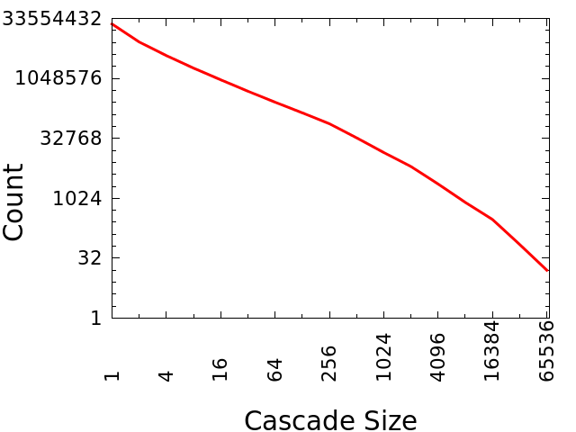
In this work any tweet that is retweeted at least once is called a cascade as it has one retweeter (or adopter) other than the original tweeter. As has been noted in prior work, most cascades are shallow (star-like) and only a rare few go on to be “viral”. We also refer to a cascade size, which is the number of eventual retweeters (or adopters) that the tweet gathers, as measured after a few days of the original tweet. In order for our analysis to be valid the dataset must be large enough to catch cascades from a spectrum of sizes. We confirm this by visually plotting the cascade size distribution in Figure 1(a), which shows the average number of cascades with size between over the 16 days. Clearly, the data has enough cascades in each bucket even for a single day.
Next, we define a tweet view or an impression on the home timeline. The ideal measurement is to check that the user really “saw” the tweet, but in absence of that, we just measure whether the tweet stayed on the user’s mobile screen for a large enough time. This filters out a variety of behaviors, and among them the common pattern of scrolling quickly through the home timeline, where the user just glances at a large number of tweets.
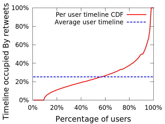
With these definitions we turn our attention to studying how much audience attention is commanded by cascades. Perhaps the most basic measurement to make is to measure what fraction of a users’ home timeline impressions came from cascades that did not originate in the user’s direct neighborhood. We find that 68% of all home timeline tweet impressions are from users’ direct followings, and the remainder 32% come from cascades that originate from outside of a users’ direct neighborhood. A different view of this overall statistic comes from looking at this from each individual user’s perspective, through which we can measure what fraction of a user’s timeline impressions come from retweets. The distribution of this quantity is shown in Figure 1(b), from which it is evident that for half of all users, approximately a quarter of their timeline consists of retweets. An additional dimension of tweet impressions coming from cascades is that these tweets bring in a fair bit of author diversity: 55% of unique authors who appear in a user’s timeline are from outside the user’s direct followings.
Given that nearly a quarter of a user’s home timeline consists of cascades, it is natural to ask how these cascades reach the user. To provide insight into this question, we look at how far away the cascade originated, and how long it took to get to the user. For the former, we measure the network distance (shortest directed path) from the user to the cascade originator (the author of the root tweet in the cascade). Table 1 shows the percentage of tweet impressions that occur for each distance (out of all impressions), and from the data it is clearly visible that almost all impressions come from within distance in the graph.
| Distance | Impressions | Hop count | Impressions | |
|---|---|---|---|---|
| 1 | 1 | |||
| 2 | 2 | |||
| 3 | 3 | |||
| 4 | 4 | |||
| 5 | 5 | |||
| 6 | 6 | |||
| 7 | 7 |
To understand the path the cascade took to reach a user, we reconstruct the cascade tree111The cascade is a directed acyclic graph from a user’s perspective, but we can think of it as a tree by picking the first incoming edge for each node by time — that is also a close approximation to how Twitter treats retweets in practice. and compute the number of hops on the tree that are between the user and the root of the tree; we refer to this quantity as the hop-count. The distribution of impressions w.r.t the hop-count is shown in Table 1. As is the case with distance, almost all impressions occur on hop counts 1 and 2. This data is all in agreement with prior work that has also commented on the vast majority of cascades being very shallow in terms of hop-count [12]. However, we do note that in contrast with distance, impressions for larger hop-counts don’t quickly die down to zero. An obvious hypothesis for this is the possibility that some large cascades survive for a long time and hence reach users via all kinds of paths. This leads to the question of the impact of these large cascades from the perspective of impressions.
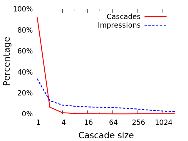
Recall that 1 out of 3 impressions arise from cascades, and in light of the previous discussion, we would like to understand which kinds of cascades are contributing to these impressions. It is useful to remember that large cascades are quite rare on Twitter, as illustrated in Figure 2(a): on a log-percentage plot, the fraction of tweets that get more than 8 retweets is less than 1%. However, since some cascades survive for a long time, it is natural to ask what is the share of impressions generated by these cascades. The share of impressions is also shown on the same Figure 2(a), and this presents a stark contrast from the probability of tweets generating a large cascade — even though 91% of tweets have a cascade size of 1, these generate only 33% of impressions coming from retweets, with the large cascades contributing a substantial fraction of impressions coming from retweets. We term this the Impressions Paradox: the share of impressions for cascades of size decays much more slowly than frequency of cascades of size .
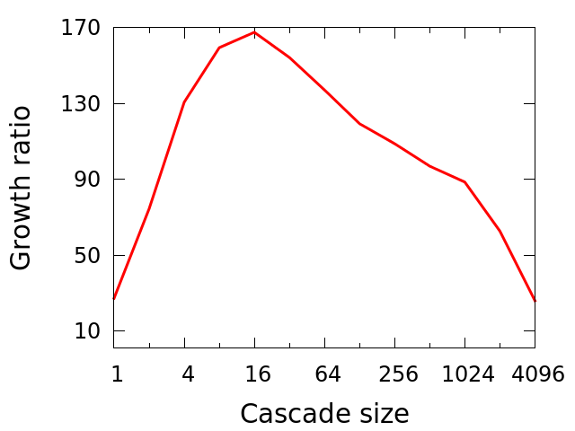
We also note that for all cascades of a given size, one can compute a cascade growth metric: the ratio between number of impressions generated by these cascades to number of tweets generated by these cascades. Intuitively, one would expect this ratio to be high for small cascades since almost every retweet brings in a large set of new audience members who haven’t seen it by other means, while for larger cascades the gain in new audience per retweet might be lower since the presence of triangles means that new retweets may eventually reach people who have already seen it by other means. In fact, from Figure 2(b), we notice that the growth ratio for cascades hits a peak around size 32, and is the same for the smallest and largest cascades!
Thus, it seems clear that even though large cascades (especially “viral” ones) are infrequent on Twitter, they constitute a substantial fraction of audience attention. This observation leads to the question of how does the audience react to the presence of cascades in their home timeline. We address this question in the next section by analyzing user engagement.
3.2 Engagement with Cascades
Users on Twitter engage with tweets in a variety of ways, and we focus on the following engagements in our analysis: retweets (resharing the tweet with your followers), likes (previously known as favoriting), and clicks (either a click on a link/mention/hashtag in a tweet, or a visit to a “tweet details” page are considered as clicks). Together, these engagements provide a broad perspective on how users perceive the content as engagements are often a reflection of how much users enjoyed the content. This is not always the case though, and engagement is skewed by a range of factors: social acceptability, context, and inherent clickability (for instance, “clickbait” may have a high clickthrough rate) of content to name a few. Despite these shortcomings, the large scale of data analysis that we conduct does provide a directional guide on user enjoyment by measuring engagement.
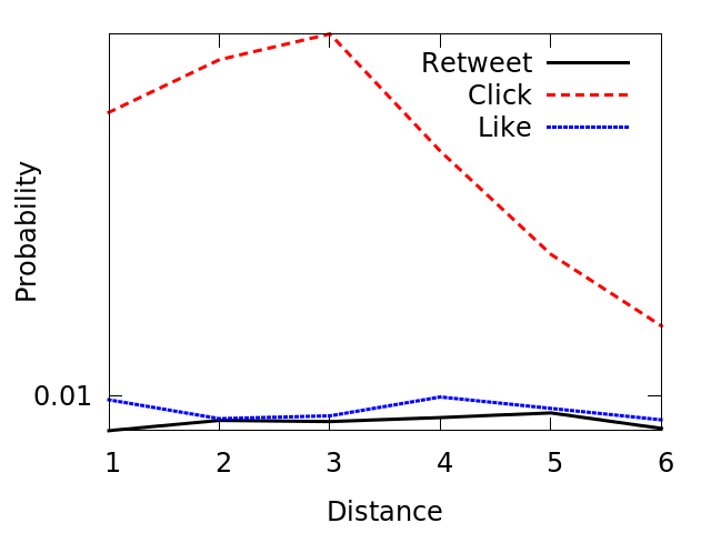
Engagement with cascades doesn’t occur in a vacuum, and here we contrast engagement on cascades against the natural baseline of engagement on “organic” tweets, i.e. tweets authored directly by a user’s followings. This comparison is readily obtained by measuring how the probability of retweets, likes and clicks varies with graph distance. These curves are presented in Figure 3, which shows that the various engagement measures behave quite differently. In particular, a tweet from a neighbor has a higher probability of receiving a like than tweets coming from users that are farther away in the network. On the other hand, a cascade tweet that originated outside of the user’s direct network has a higher chance of getting retweeted and clicked. This perhaps is an indication that liking has a social element to it, and users tend to primarily like personalized content or tweets that come from their direct neighbors. On the other hand, a tweet that arrives in a cascade from outside the neighborhood is “retweetable” by definition, and hence just by this selection mechanism it increases its chances of getting retweeted as compared to an average tweet that may not received any retweets at all. The click probability curve shows different behavior than both likes and retweets, and the probability of clicking on the tweet increases till distance 3. It is important to point out that to a consumer on Twitter, the only visible distinction in distance is whether it is 1 (direct connection) or greater (retweet). Thus, the difference between click probability in distances 2 and beyond likely comes from something other than user selectiveness between in and out of network content. An appealing hypothesis is that perhaps inherently clickable content travels farther on the network. We examine this next via a hop count analysis.
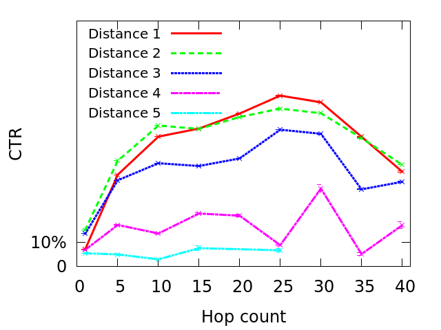
Recall that hop-count refers to the distance from the user to the author in the cascade tree. In order to understand the click probability variation, we turn to examining click-through rate (CTR) of tweets by hop-count — since this route is predominantly available to larger cascades, it provides us a way to measure how users react to large cascades versus other smaller cascades. This data is presented in Figure 4, where there is a curve for a fixed distane showing the average CTR of tweets based on the hop-count value. There are several things to notice in this plot. First, observe that for a fixed hop-count, CTR generally decreases with distance — this clarifies that the increase with distance observed in Figure 3 is at least partially due to an effect that it to some extent like Simpson’s paradox. We also note from Figure 4 that CTR generally increases with hop-count. Recall that higher hop counts are generally only available to large cascades, and hence the higher CTR indicates that popular content generates more clicks. We emphasize that this is not a causal statement, and in particular popular content might precisely be more popular because it generates more clicks.
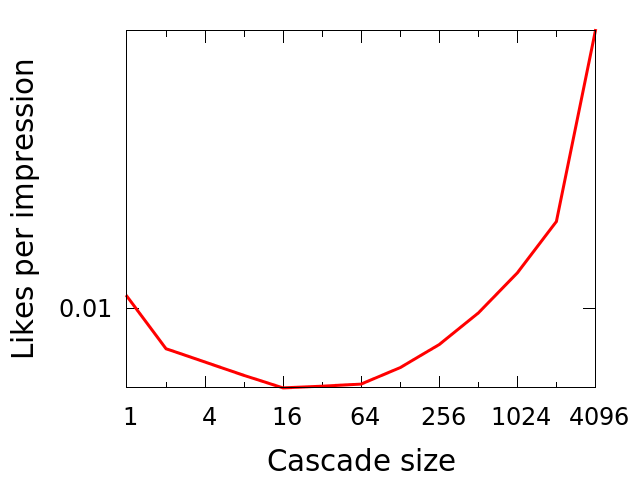
Given this data, we are left with the intriguing observation that users enjoy consuming (via liking/clicking) content both from their direct neighbors as well as from large cascades. But the combined effect of these two mechanisms is apriori unclear. In particular, since large cascades can travel farther from their source, does their overall appeal overcome the fact that their audience is not their direct neighbors? The most direct way to study this question is to look at like probability per tweet impression based on the cascade size of the tweet, and Figure 5(a) shows the result of this investigation. Note that the cascades are bucketed as before, since the number of cascades with large sizes are rare. We observe from Figure 5(a) that cascades with very small and very large sizes have high like per impression rates. These stand in contrast with a smaller like per impression value for medium size cascades. We can thus see the two mechanisms mentioned above at play here: at small cascade sizes, content is being liked by neighbors (perhaps driven by a social aspect), while at large sizes content is likeable in general so most users enjoy consuming it. But there is an “uncanny valley” in the middle where not naturally likeable content reaches users who are not quite interested in it. The connection between Figure 2(b) and 5(a) is very interesting, and we leave further investigation of this connection as a direction for future work.
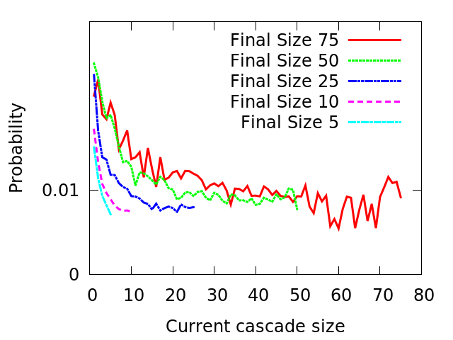
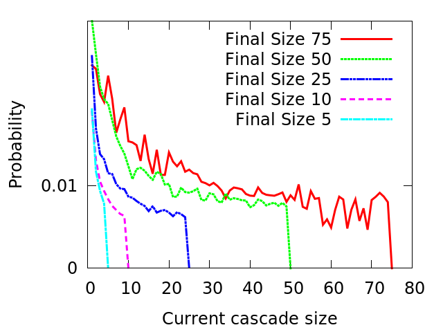
From 5(a), it seems clear that the most popular content, as indicated by size, has the highest like rate. Since users on Twitter can see the overall popularity of a tweet (the number of retweets and likes), size does provide a signaling mechanism that could potentially bias the highest like rate in the favor of popular tweets, fueling a rich-gets-richer effect. Another possibility is that tweets have an intrinsic “quality” that drives their popularity and higher size is partially a result of this quality (it could still involve other factors too, such as being lucky and receiving attention from popular users early in the tweet’s lifetime). To disambiguate between these possibilities, we observe that over the lifetime of a cascade, different users view the tweet at different points in its popularity. This allows us to study whether users react differently to tweets that had different eventual sizes but were viewed at the same level of popularity by users. We can see from results in Figure 6 that the cascades that ended up with a larger eventual size had a higher like and retweet rate even earlier in their life. This provides some evidence that intrinsic quality of a tweet does contribute to its eventual popularity.
3.2.1 Individual User Preferences
The analysis above suggests that globally popular content is also locally popular at an aggregate level for users. We now examine individual user variation for these preferences: do most users like globally popular content? Are users consistent in their preferences on local vs global content? In order to study these questions, we randomly selected active users on Twitter, where if a user had at least one interaction each day for more than days out of a day period in June, we count him/her as an active user.
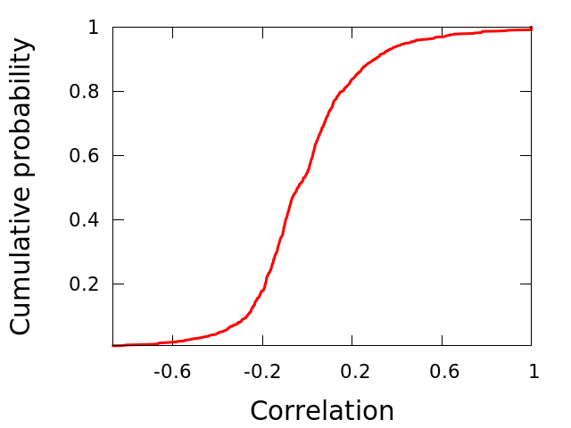
Let us first turn to the question of local vs global preference for a user. To study this, for each user we compute the Pearson correlation coefficient between the final cascade size and like probability of all the tweets that the user viewed in this period. The distribution of these correlations over the users is shown in Figure 5(b). As we see from the plot, most users have a negative correlation, implying that they prefer personalized content. However, the correlation coefficient is low for these negatively correlated users, and if we only focus instead on users who have strong correlation then most of these are positively correlated. In either case, users do seem to exhibit a local/global content preference.
The local/global preference as expressed by a correlation is however rather weak, and leaves open the question of whether users are consistent in their preferences. Here, we study user consistency via the following analysis. We define the function , for user , day and any , to be the fraction of likes produced by the fraction of smallest cascades that user sees on day . If , it means that user likes content that is part of smaller cascades at a greater rate than they like content that is part of larger cascades; we could think of this as the user liking personal content more than broadly-shared general content. The implication is the opposite if the inequality is reversed: if , then the user like content that it part of large cascades (and hence more broadly-shared general content) at a greater rate. We operationalize this definition by identifying users who like small (respectively, large) cascades according to the condition (respectively ).
| Consistent small cascade liker | 19.4% |
|---|---|
| Consistent big cascade liker | 47.1% |
| Indifferent | 33.5% |
Further, if a user likes the same type of cascades at least days over the day period, we call her a consistent user (either a liker or large cascades or a liker of small cascades); otherwise we call her indifferent. With this definition of consistency, we find that more than of our users are consistent. The fraction of users of each type can be seen in Table 2. As a simple baseline, note that if each user independently decided each day with uniform probability whether to like small cascades or large cascades, we’d expect only of all users to be consistent, rather than over 66% as we find in the data.
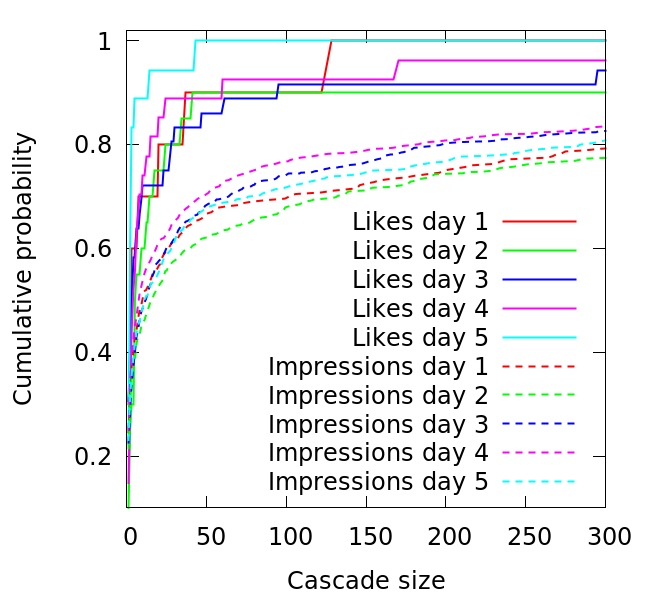
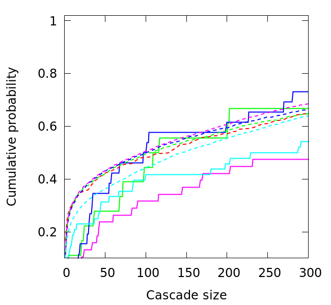
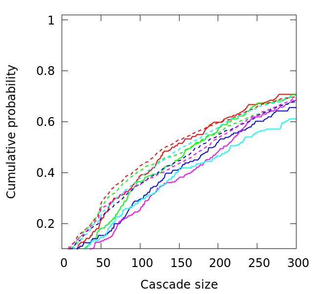
We also provide a useful illustration of how these three user behaviors are distinct. We define () to be the fraction of impressions (likes) that user had on day and the cascade sizes were less than . We then show how these two functions behave for all three types of users (prefers personal content, broader content or indifferent) in Figure 7. We draw the function with dashed line and with solid lines. This data clearly indicates that users do indeed have consistently different preferences, which might stem from using Twitter for different purposes. We leave a more in-depth investigation of this to future work, but note that Twitter does exhibit both social and information network structural properties indicating the presence of multiple usage scenarios [17].
We now summarize our overall empirical findings: cascades have a large audience on Twitter, larger than one might expect just based on cascade occurrence (cf. the Impressions Paradox). Furthermore, users seem to like these cascades, even relative to organic content. However, these observations seem to be somewhat at odds with each other: since a lot of users see large cascades, either cascading content is always appreciated by a large majority or somehow it reaches predominantly users who would enjoy it. The latter possibility is what we explore in the remainder of this work, with the lens of a simple theoretical model.
4 Modeling Cascades For Audience
The empirical analysis presented earlier leads to the conclusion that a quarter of a typical user’s timeline consists of retweets, and users find this content engaging. As we’ve alluded to before, this presents a conflict between the view of users choosing exactly what content they want to see (by following a set of users) and engaging content being bubbled up through the network via retweets. In this section, we posit a simple theoretical model that shows this conflict can be resolved in a natural manner by users being selective about content they retweet. We emphasize that the model is purposely bare-bones so that it can provide stylized insight into why cascades turn out to be relevant for users.
The main idea of our model is to think of an inverted tree where a member of the audience (a consumer of cascades) is the root, in contrast to the standard view of the cascade originator as the root node. This allows us to examine the path that content takes to arrive at the audience member at the root node. The model includes a notion of topic, which governs whether a given user is interested in a given tweet. We can now define the model formally using these notions.
Each user in the network has a set of topics they are interested in: , where and the set contains the universe of topics (). For a fixed arbitrary user , we consider their two-hop neighborhood (recall from Table 1 that vast majority of the retweets arrive from two hops away): follows the set of users , and each user follows , with the entire second hop neighborhood being denoted by . In this simple network, we assume that if a user follows user , then is interested in a significant fraction of ’s topics. More formally, we assume that for a fixed constant , . We’ll shortly address the question of how this extended neighborhood is generated, but first we will focus on the cascade process given such a network.
Given a network that has content being produced and consumed on it, for each user we will have a “home timeline” which is populated by content produced by the set of users that follows; we denote the set of tweets in ’s home timeline by . We now specify the content production process. First, we link users’ topical interests to tweets by assigning a single topic to each tweet , where is selected from the author’s list of topics. We also assume that tweet has an intrinsic quality , which is in line with our observations from Figure 6. For tweet production, we assume simplistically that at all users produce tweets at each epoch as follows. First, each user creates an original candidate tweet on one of the topics , with a quality drawn from a specified distribution , but doesn’t publish this candidate to its followers yet. The user picks her tweet that she will publish as follows: she considers her own tweet and her home timeline — consisting of tweets produced in the previous epoch by the users she follows — and then among the tweets in this set for which , she selects the tweet of highest quality
This setting reflects the fact that users can both participate in cascades as well as produce original content. Further, the model allows for user curation for cascades that biases towards participation in higher quality cascades. The goal of the model is to capture the consumer viewpoint on cascades, and the consumer view is governed by whether the content in their home timeline is high quality, and also on whether it is on a topic that is interesting to them. We formally define these metrics for the home timeline of a given user as follows:
Definition 4.1 (Precision)
We define precision for a user as the fraction of tweets in ’s timeline that would be interested in: .
Definition 4.2 (Quality)
We define the timeline quality for a user as the average quality of all tweets in ’s home timeline: .
Definition 4.3 (Timeline Utility (TLU))
If is the quality coefficient for tweets that are not on topic for the consumer then the overall timeline utility of the home timeline for a given user , can be defined as
Here if , and otherwise. Thus, increases if there are high-quality tweets and decreases if there are off-topic tweets.
Thus, the model aims to capture the effect of cascades on the twin goals of having users enjoy both high quality and precise content. Intuitively, retweets seem to filter for high quality tweets but the effect on precision is less clear. In fact, the exact effect on precision depends on network topology. We now define how the network is created, starting with a simple model that is analytically tractable. We’ll later define a more complex model on which we simulated the model.
Possibly the simplest way to construct a network is to build a tree. We proceed by having given the node for which we want to study the above metrics, and her corresponding topical interests. Then we pick random interest sets that satisfies the homophily condition (of fraction interest overlap), and designate those to be the interest sets of the nodes in . We then repeat the same procedure for each and create neighbors for each while also satisfying the homophily restrictions. Given this network generation model, now we can analyze the effect of cascades on previously defined quality and precision metrics.
For the theoretical analysis we look into a basic setting where . In the next subsection we remove these restrictions and report the results on the simulation. We begin by noting that based on the graph generation process, the distribution of topics in on the topics in is uniform. Now, in every epoch but the first (once retweets start moving through the network), the view of a node is as follows. If receives a tweet that she is not interested in, that has no chance of being propagated. Otherwise, she will keep the tweet as a candidate in the maximization step. Now, we know that the distribution of the tweet topics coming from is uniform on , so we observe that the model is equivalent to itself generating many tweets and only publishing the best. If we look at the process in this manner, then it is clear that the expected precision does not change when we introduce retweets. However, with this procedure the quality of tweets will go up. It is easy to see that the expected quality of a single tweet is less than the expectation of the maximum of independent draws from the same distribution. We formalize the gain in quality for two specific distributions, and note that the analysis can be extended to other distributions.
In particular we investigate the two cases where is either a uniform distribution over or an exponential distribution with rate . We use to refer to the distribution of the maximum of draws from . A question we want to answer is; how much do retweets help the quality of the timeline to increase? Let be a random variable drawn from and be a random variable drawn from . With our notation we are interested in . It is well known that the mean of a uniform distribution over is and the mean of a exponential distribution of rate is . Now we state two well-known lemmas about the maximum of a set of independent draws from a fixed distribution [20].
Lemma 4.4
The expectation of the maximum of i.i.d draws from a uniform distribution over is .
Lemma 4.5
The expectation of the maximum of i.i.d draws from an exponential distribution of rate is , where is the -th harmonic number.
We can now state the main theoretical result on the effect of retweets on quality. We skip by proof but note that it is easily obtained from the above two lemmas.
Theorem 4.6
The multiplicative increase in quality in the scenario where is uniform is and when is an exponential distribution with rate , it is .
The theorem formalizes the gain in quality that comes from having cascades in the network, which is a counterfactual that is not easily observable in the Twitter network222This remains hard to measure even via experimentation as there is a large network effect to contend with.. To gain some sense of the scale of this increase, let us consider a network where the average degree of nodes is (This number is a lower-bound for the Twitter network). By plugging in for we see that the uniform and exponential distribution model yield a and increase in quality, respectively! This shows how valuable retweets can be to a network, as illustrated by our stylized model. We re-emphasize that we do not claim our theorem to be representative of the gain in the Twitter setting — the goal of this modeling exercise is to shed light on the effect of cascades on the audience, and we can quantify that effect with the help of a formal model. We now explore generalizing this model by removing some assumptions.
4.1 Model Extensions
The above model is quite simple and makes a few strong assumptions in order to be analytically tractable. In this section, we explore the effect of removing or generalizing these assumptions via simulating the model. In particular, there are two obvious ways we can generalize the model.
First, we previously assumed that the two-hop graph was a tree, but now we generalize that to the following two graphs:
-
Tree Contracted model: Here, we create the graph using the Tree model but contract all the nodes in layer and that have the same interest set into one single node.
-
-NN: Here, we create a number of nodes333For our simulations, we use nodes. with their own interest set, and each person follows the people that have the most common interests with them. (We break ties in this choice of at random.)
Second, we can change various aspects of the model in the previous section, which includes both changing existing parameter values and generalization of behavior from the model in the previous section. The generalizations we examine are as follows:
-
: Recall that if a user receives an off-topic tweet of quality , then she sees that as a tweet with quality . This parameter is used for both in finding the and the retweeting procedure, and was previously set to 1. Here, we explore the effect of using other values for .
-
: This parameter allows us to control the average degree of the neighbors of the target node to her degree. We note that in our simulations, the results stabilize once this ratio is above , and this value is above 20 for Twitter in particular.
-
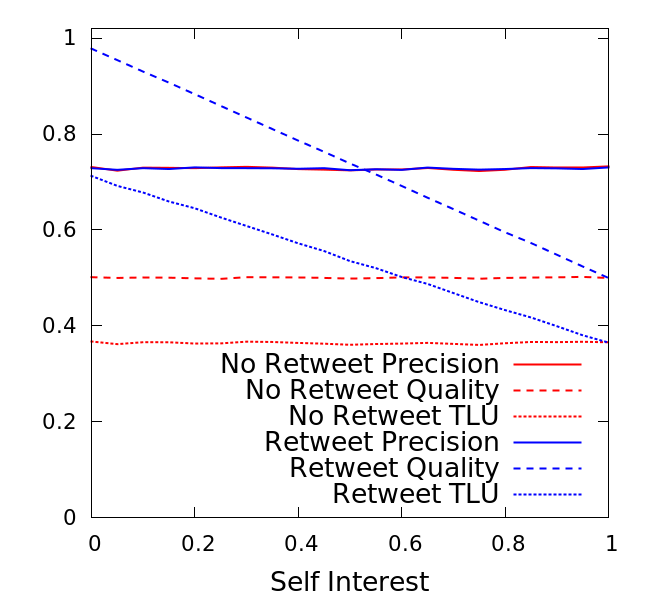
The self-interest factor (p): We introduce a new parameter to allow users the flexibility to tweet original content instead of simply retweeting others. We stipulate that in each epoch, a user tweets her own tweet with probability , and otherwise, retweets one of the tweets that she has received. Also, when retweeting the user differentiates between the tweets from the people she follows and the people that she does not follow (We take following to be a proxy for knowing). Thus, once she decides to retweet someone, with probability she picks the highest quality tweet created by one of her immediate followees, otherwise she picks the highest quality tweet from the pool of tweets coming from more than one hop away from her.
Note that as we increase , this method creates a bias towards (i) creating her own organic tweet, and (ii) while retweeting, she prioritizes her immediate neighbors’ tweet over tweets coming from deeper in the network. This creates a mechanism that constructs timelines which most of its content is from at most two hops away.
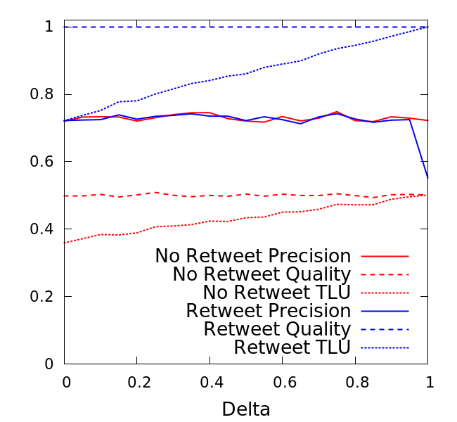
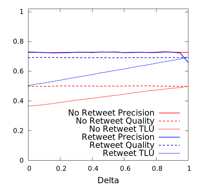
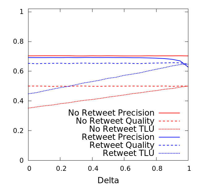
The simulations results from varying the network model and the above parameters are all shown in Figure 8. From the results, we observe that the following holds unless is close to 444Recall that being close to 1 would imply users not distinguishing between on and off topic tweets, and hence it makes sense to focus on results where is smaller than 1.: by introducing retweets in the network, the precision remains essentially the same and the quality goes up, leading to a higher . This is quite consistent with the theorem in the previous section and shows that the observations in the previous section are somewhat robust to the specific network model and parameters.
5 Conclusions
Information cascades on networks affect not only the users who actively participate in them, but also the audience who are consequently exposed to the cascades. Our work provides a view of cascades from the point of view of the audience, which has not received much attention to the best of our knowledge. Our findings related to the Impressions Paradox provides a novel perspective for future work on the effect of cascades on their audience.
The theoretical model presented here is quite simplistic, but it does highlight the crucial role of cascade participants as gatekeepers of precision. In addition to further generalizations of the model, this work raises several additional open questions for future work. Clearly, not all users retweet on topic, but does the network rewire itself (via audience following/unfollowing) so that precision remains high? Furthermore, an aspect of cascades we did not discuss here is their usefulness as a discovery mechanism; can effective discovery coexist with high precision in the network?
Healthy dynamics on social networks requires both active producers and engaged consumers. We believe our work provides a novel and useful consumer counterpoint to the extensive literature on the role that producers play in cascades.
References
- [1] L. A. Adamic and N. Glance. The political blogosphere and the 2004 us election: divided they blog. In International workshop on Link discovery. ACM, 2005.
- [2] R. Arratia and L. Goldstein. Size bias, sampling, the waiting time paradox, and infinite divisibility: when is the increment independent? Technical Report 1007.3910, arxiv.org, Oct. 2007.
- [3] E. Bakshy, S. Messing, and L. Adamic. Exposure to ideologically diverse news and opinion on Facebook. Science, 5 2015.
- [4] L. Barone. Why twitter’s new retweet feature sucks. http://outspokenmedia.com/social-media/twitters-new-retweet-feature-sucks/. 2009, Accessed: 2016-08-20.
- [5] J. Berger and K. L. Milkman. What makes online content viral? Journal of Marketing Research, 2012.
- [6] R. Bosagh Zadeh, A. Goel, K. Munagala, and A. Sharma. On the precision of social and information networks. In Proceedings of the first ACM conference on Online social networks, pages 63–74. ACM, 2013.
- [7] J. Cheng, L. A. Adamic, P. A. Dow, J. M. Kleinberg, and J. Leskovec. Can cascades be predicted? In Proc. 23rd WWW, pages 925–936, 2014.
- [8] C. Danescu-Niculescu-Mizil, J. Cheng, J. Kleinberg, and L. Lee. You had me at hello: How phrasing affects memorability. In Proceedings of the ACL. Association for Computational Linguistics, 2012.
- [9] P. A. Dow, L. A. Adamic, and A. Friggeri. The anatomy of large facebook cascades. In ICWSM, 2013.
- [10] Facebook. News Feed FYI: helping make sure you Don’t miss stories from friends. http://newsroom.fb.com/news/2016/06/news-feed-fyi-helping-make-sure-you-dont-miss-stories-from-friends/. Accessed: 2016-10-24.
- [11] A. Goel, K. Munagala, A. Sharma, and H. Zhang. A note on modeling retweet cascades on twitter. In International Workshop on Algorithms and Models for the Web-Graph, pages 119–131. Springer International Publishing, 2015.
- [12] S. Goel, A. Anderson, J. Hofman, and D. J. Watts. The structural virality of online diffusion. Management Science, 62(1):180–196, 2015.
- [13] S. Goel, A. Anderson, J. M. Hofman, and D. J. Watts. The structural virality of online diffusion. Management Science, 62(1):180–196, 2016.
- [14] J. Leskovec, L. Adamic, and B. Huberman. The dynamics of viral marketing. ACM Transactions on the Web, 2007.
- [15] Y.-R. . R. Lin, D. Margolin, B. Keegan, A. Baronchelli, and D. Lazer. #bigbirds never die: Understanding social dynamics of emergent hashtag. In ICWSM, 3 2013.
- [16] S. K. Maity, R. Saraf, and A. Mukherjee. # bieber+# blast=# bieberblast: Early prediction of popular hashtag compounds. In Proceedings of CSCW, 2016.
- [17] S. A. Myers, A. Sharma, P. Gupta, and J. Lin. Information network or social network?: the structure of the twitter follow graph. In Proceedings of the 23rd International Conference on World Wide Web, pages 493–498. ACM, 2014.
- [18] D. M. Romero, B. Meeder, and J. Kleinberg. Differences in the mechanics of information diffusion across topics: Idioms, political hashtags, and complex contagion on Twitter. In Proceedings of WWW, pages 695–704, 2011.
- [19] D. M. Romero, C. Tan, and J. Ugander. On the interplay between social and topical structure. In Proceedings of ICWSM, 2013.
- [20] S. M. Ross. Introduction to Probability Models, Ninth Edition. Academic Press, Inc., Orlando, FL, USA, 2006.
- [21] O. Tsur and A. Rappoport. What’s in a hashtag?: content based prediction of the spread of ideas in microblogging communities. In Proceedings of the fifth ACM international conference on Web search and data mining. ACM, 2012.
- [22] Twitter. While you were away… https://blog.twitter.com/2015/while-you-were-away-0. Accessed: 2016-10-24.
- [23] S. Wu, J. M. Hofman, W. A. Mason, and D. J. Watts. Who says what to whom on twitter. In Proceedings of the 20th International Conference on World Wide Web, WWW ’11, pages 705–714, New York, NY, USA, 2011. ACM.
