aainstitutetext: Deutsches Elektronen-Synchroton DESY, Notkestraße 85, 22607 Hamburg, Germanybbinstitutetext: Nikhef Theory Group and VU University Amsterdam, De Boelelaan 1081, 1081 HV Amsterdam, The Netherlandsccinstitutetext: Deutsches Elektronen-Synchrotron DESY, Platanenallee 6, 15738 Zeuthen, Germany

Double hard scattering without double counting

Markus Diehl b    Jonathan R. Gaunt c    and Kay Schönwald markus.diehl@desy.de jgaunt@nikhef.nl kay.schoenwald@desy.de
Abstract

Double parton scattering in proton-proton collisions includes kinematic regions in which two partons inside a proton originate from the perturbative splitting of a single parton. This leads to a double counting problem between single and double hard scattering. We present a solution to this problem, which allows for the definition of double parton distributions as operator matrix elements in a proton, and which can be used at higher orders in perturbation theory. We show how the evaluation of double hard scattering in this framework can provide a rough estimate for the size of the higher-order contributions to single hard scattering that are affected by double counting. In a numeric study, we identify situations in which these higher-order contributions must be explicitly calculated and included if one wants to attain an accuracy at which double hard scattering becomes relevant, and other situations where such contributions may be neglected.

1 Introduction

The precise description of high-energy proton-proton collisions in QCD is imperative for maximising the physics potential of the LHC and of possible future hadron colliders. An important issue in this context is to understand the mechanism of double parton scattering (DPS), in which two pairs of partons undergo a hard scattering in one and the same proton-proton collision. In many situations DPS is suppressed compared with single parton scattering (SPS), but this suppression generically becomes weaker with increasing collision energy. For specific kinematics or specific final states, DPS can become comparable to or even larger than SPS. An overview of recent experimental and theoretical activities in this area can for instance be found in Astalos:2015ivw ; Proceedings:2016tff .

Consider a DPS process ppY1+Y2+X𝑝𝑝subscript𝑌1subscript𝑌2𝑋pp\to Y_{1}+Y_{2}+X, where Y1subscript𝑌1Y_{1} and Y2subscript𝑌2Y_{2} are observed particles or groups of particles produced in two separate hard scattering processes, whilst X𝑋X denotes all unobserved particles in the final state. A cross section formula has been put forward long ago in the framework of collinear factorisation, where the transverse momenta 𝒒1subscript𝒒1\boldsymbol{q}_{1} and 𝒒2subscript𝒒2\boldsymbol{q}_{2} of Y1subscript𝑌1Y_{1} and Y2subscript𝑌2Y_{2} are integrated over Paver:1982yp . A corresponding expression has been given in Diehl:2011tt ; Diehl:2011yj for transverse momentum dependent (TMD) factorisation, where 𝒒1subscript𝒒1\boldsymbol{q}_{1} and 𝒒2subscript𝒒2\boldsymbol{q}_{2} are small compared with the hard scales in Y1subscript𝑌1Y_{1} and Y2subscript𝑌2Y_{2}.

Inside a proton, the two partons that take part in the two hard scatters can originate from the perturbative splitting of one parton. The relevance of this splitting mechanism for the evolution equations of double parton distributions (DPDs) has been realised long ago Kirschner:1979im ; Shelest:1982dg and studied more recently in Snigirev:2003cq ; Gaunt:2009re ; Ceccopieri:2010kg . However, it was only noted in Diehl:2011tt ; Diehl:2011yj that the same mechanism dominates DPDs in the limit of small transverse distance between the two partons, and that the splitting contribution leads to infinities when inserted into the DPS cross section formula. These infinities are closely connected with double counting between DPS and SPS in particular Feynman graphs, a problem that had been pointed out earlier in the context of multi-jet production Cacciari:2009dp .

Different ways of dealing with this issue have been proposed in Blok:2011bu ; Blok:2013bpa , Ryskin:2011kk ; Ryskin:2012qx and Manohar:2012pe . As discussed later in this paper, we find that these proposals have shortcomings either of theoretical or of practical nature. In the present work we present an alternative scheme for computing the cross section in a consistent way, including both DPS and SPS (as well as other contributions). Our scheme allows for a nonperturbative definition of DPDs in terms of operator matrix elements, and it is suitable for pushing the limit of theoretical accuracy to higher orders in αssubscript𝛼𝑠\alpha_{s}.

Our paper is structured as follows. In section 2 we recall the theoretical framework for describing DPS and specify the theoretical problems mentioned above. The short-distance behaviour of DPDs is discussed in section 3, since it is essential for the scheme we propose in section 4. We first show how this scheme works at leading order (LO) in αssubscript𝛼𝑠\alpha_{s}, before giving examples of its application at next-to-leading order (NLO) in section 5. Collinear DPDs evolve according to DGLAP equations, and in section 6 we discuss several consequences of this scale evolution. Our scheme is naturally formulated with DPDs that depend on the transverse distance 𝒚𝒚\boldsymbol{y} between the two partons, but we show in section 7 how one may instead use DPDs depending on the transverse momentum conjugate to 𝒚𝒚\boldsymbol{y}. This allows us to compare our results with those of Blok:2011bu ; Blok:2013bpa and Ryskin:2011kk ; Ryskin:2012qx , which we do in section 8. Whilst the focus of the present work is theoretical rather than phenomenological, we give in section 9 some quantitative illustrations of our scheme, obtained with a relatively simple ansatz for the DPDs. We summarise our findings in section 10. Some Fourier integrals required in the main text are given in an appendix.

2 Setting the scene

In this section we recall theoretical issues originating from the perturbative splitting mechanism in double parton distributions, namely the appearance of ultraviolet divergences in the naive cross section for double parton scattering, the problem of double counting between DPS and single parton scattering, and the treatment of the so-called 2v1 (two versus one) contributions to DPS.111We follow here the nomenclature of Gaunt:2012dd . The 2v1 contribution is referred to as 4×2424\times 2 in Diehl:2011yj , as 34343\to 4 in Blok:2011bu ; Blok:2013bpa (where four-jet production is considered), and as 1×2121\times 2 in Ryskin:2011kk ; Ryskin:2012qx . We also give some basic definitions and results. Throughout this work we use light-cone coordinates v±=(v0+v3)/2superscript𝑣plus-or-minussuperscript𝑣0superscript𝑣32v^{\pm}=(v^{0}+v^{3})/\sqrt{2} for any four-vector v𝑣v. We write 𝒗=(v1,v2)𝒗superscript𝑣1superscript𝑣2\boldsymbol{v}=(v^{1},v^{2}) for the transverse components and v=𝒗2𝑣superscript𝒗2v=\sqrt{\boldsymbol{v}^{2}} for the length of the transverse vector.

Since the perturbative splitting mechanism in DPDs leads to issues in the ultraviolet (UV) region, renormalisation plays a crucial role in our context. We work in dimensional regularisation and extend the definitions of Diehl:2011yj to D=42ϵ𝐷42italic-ϵD=4-2\epsilon dimensions, changing phase space factors (2π)4superscript2𝜋4(2\pi)^{4} into (2π)Dsuperscript2𝜋𝐷(2\pi)^{D}. Bare two-parton distributions are then given by

Fbare(xi,𝒛i,𝒚)subscript𝐹baresubscript𝑥𝑖subscript𝒛𝑖𝒚\displaystyle F_{\text{bare}}(x_{i},\boldsymbol{z}_{i},\boldsymbol{y}) =2p+𝑑ydz12πdz22πei(x1z1+x2z2)p+p|𝒪2(0,z2)𝒪1(y,z1)|pabsent2superscript𝑝differential-dsuperscript𝑦𝑑superscriptsubscript𝑧12𝜋𝑑superscriptsubscript𝑧22𝜋superscript𝑒𝑖subscript𝑥1superscriptsubscript𝑧1subscript𝑥2superscriptsubscript𝑧2superscript𝑝quantum-operator-product𝑝subscript𝒪20subscript𝑧2subscript𝒪1𝑦subscript𝑧1𝑝\displaystyle=2p^{+}\!\!\int dy^{-}\int\frac{dz_{1}^{-}}{2\pi}\,\frac{dz_{2}^{-}}{2\pi}\,e^{i(x_{1}z_{1}^{-}+x_{2}z_{2}^{-})p^{+}}\bigl{\langle}p\mskip 1.5mu|\mskip 1.5mu\mathcal{O}_{2}(0,z_{2})\,\mathcal{O}_{1}(y,z_{1})\mskip 1.5mu|\mskip 1.5mup\bigr{\rangle} (1)

with twist-two operators

𝒪i(y,zi)subscript𝒪𝑖𝑦subscript𝑧𝑖\displaystyle\mathcal{O}_{i}(y,z_{i}) =q¯(y12zi)W(y12zi)ΓiW(y+12zi)q(y+12zi)|zi+=y+=0absentevaluated-at¯𝑞𝑦12subscript𝑧𝑖superscript𝑊𝑦12subscript𝑧𝑖subscriptΓ𝑖𝑊𝑦12subscript𝑧𝑖𝑞𝑦12subscript𝑧𝑖superscriptsubscript𝑧𝑖superscriptsubscript𝑦absent0\displaystyle=\bar{q}\bigl{(}y-{\tfrac{1}{2}}z_{i}\bigr{)}\mskip 1.5muW^{\dagger}\bigl{(}y-{\tfrac{1}{2}}z_{i}\bigr{)}\Gamma_{i}\mskip 1.5muW\bigl{(}y+{\tfrac{1}{2}}z_{i}\bigr{)}\mskip 1.5muq\bigl{(}y+{\tfrac{1}{2}}z_{i}\bigr{)}\big{|}_{z_{i}^{+}=y_{\phantom{z}}^{+}=0} (2)

for quark distributions, where q𝑞q denotes the bare field. W(z)𝑊𝑧W(z) is a Wilson line from z𝑧z to infinity along a prescribed path, which we do not recall here. The Dirac matrices ΓisubscriptΓ𝑖\Gamma_{i} select different quark polarisations. Analogous definitions hold for distributions involving gluons, with quark fields replaced by gluon field strength operators. For ease of writing, we omit colour labels on the operators and distributions throughout this work, bearing in mind that different colour couplings are possible for the four parton fields in (1).

In the process of deriving factorisation, one finds that the proton matrix element in (1) needs to be multiplied by a combination of so-called soft factors, which are vacuum expectation values of products of Wilson lines. More information for the case of single parton distributions can be found in chapter 13.7 of Collins:2011zzd and in the recent overview Rogers:2015sqa . A brief account for DPDs is given in section 2.1 of Diehl:2015bca , and a more detailed discussion will be provided in Buffing:2016wip . The product Fbare×{soft factors}subscript𝐹baresoft factorsF_{\text{bare}}\times\{\text{soft factors}\} depends on a parameter ζ𝜁\zeta which regulates rapidity divergences. A scheme in which a soft factor appears explicitly in the cross section formula was presented in Manohar:2012jr . Since the treatment of soft gluons does not affect parton splitting in any special way, we will not discuss it further in the present paper. Correspondingly, we will suppress the argument ζ𝜁\zeta in all DPDs.

As a final step one performs UV renormalisation, which we assume to be done in the MS¯¯MS\overline{\text{MS}} scheme. The DPDs obtained from (1) are appropriate for TMD factorisation, with the transverse positions 𝒛isubscript𝒛𝑖\boldsymbol{z}_{i} being Fourier conjugate to the transverse parton momenta that determine the final state kinematics. These distributions renormalise multiplicatively, with one renormalisation factor for each product of a quark field (or gluon field strength) with the Wilson line at the same transverse position and one factor for each pair of Wilson lines at the same transverse position in the soft factors. Denoting the product of these factors with Z𝑍Z, one obtains the final DPD as F=limϵ0(Z×Fbare×{soft factors})𝐹subscriptitalic-ϵ0𝑍subscript𝐹baresoft factorsF=\lim_{\epsilon\to 0}\bigl{(}Z\times F_{\text{bare}}\times\{\text{soft factors}\}\bigr{)}. It obeys a renormalisation group equation which is a straightforward generalisation of the one for TMDs (given e.g. in  Rogers:2015sqa ).

The DPDs needed for collinear factorisation are obtained by setting 𝒛i=𝟎subscript𝒛𝑖0\boldsymbol{z}_{i}=\boldsymbol{0} in Fbaresubscript𝐹bareF_{\text{bare}} and in the associated soft factors, before renormalisation. Setting 𝒛i=𝟎subscript𝒛𝑖0\boldsymbol{z}_{i}=\boldsymbol{0} introduces ultraviolet divergences in the operators 𝒪1subscript𝒪1\mathcal{O}_{1} and 𝒪2subscript𝒪2\mathcal{O}_{2}, and in the associated soft factors. The renormalised DPDs are then obtained as F=limϵ0(Z1Z2Fbare×{soft factors})𝐹subscriptitalic-ϵ0tensor-productsubscript𝑍1subscript𝑍2subscript𝐹baresoft factorsF=\lim_{\epsilon\to 0}\bigl{(}Z_{1}\otimes Z_{2}\otimes F_{\text{bare}}\times\{\text{soft factors}\}\bigr{)}, where Zisubscript𝑍𝑖Z_{i} renormalises the operators associated with parton i𝑖i and where the convolution products are in the momentum fractions xisubscript𝑥𝑖x_{i}. In the colour singlet channel, where both operators 𝒪isubscript𝒪𝑖\mathcal{O}_{i} in (1) are colour singlets, the soft factors reduce to unity and one obtains the renormalised twist-two operators that appear in single parton densities.

Since the operators associated with partons 111 and 222 renormalise independently (both for the TMD and the collinear case) one may choose different renormalisation scales μ1subscript𝜇1\mu_{1} and μ2subscript𝜇2\mu_{2} in each of them. This is useful when the two hard subprocesses in double parton scattering have widely different hard scales. In particular, one can then approach the kinematics of the so-called underlying event, with a very hard scattering at scale μ1subscript𝜇1\mu_{1} and additional jet production at a much lower scale μ2subscript𝜇2\mu_{2} (of course μ2subscript𝜇2\mu_{2} needs to remain in the perturbative region for our factorisation approach to be justified).

With different scales μ1,μ2subscript𝜇1subscript𝜇2\mu_{1},\mu_{2} in the collinear DPDs, we have a homogeneous evolution equation

ddlogμ12Fa1a2(x1,x2,𝒚;μ1,μ2)𝑑𝑑superscriptsubscript𝜇12subscript𝐹subscript𝑎1subscript𝑎2subscript𝑥1subscript𝑥2𝒚subscript𝜇1subscript𝜇2\displaystyle\frac{d}{d\log\mu_{1}^{2}}\,F_{a_{1}a_{2}}(x_{1},x_{2},\boldsymbol{y};\mu_{1},\mu_{2})
=b1x11x2dx1x1Pa1b1(x1x1,αs(μ1))Fb1a2(x1,x2,𝒚;μ1,μ2)absentsubscriptsubscript𝑏1superscriptsubscriptsubscript𝑥11subscript𝑥2𝑑superscriptsubscript𝑥1superscriptsubscript𝑥1subscript𝑃subscript𝑎1subscript𝑏1subscript𝑥1superscriptsubscript𝑥1subscript𝛼𝑠subscript𝜇1subscript𝐹subscript𝑏1subscript𝑎2superscriptsubscript𝑥1subscript𝑥2𝒚subscript𝜇1subscript𝜇2\displaystyle\qquad=\sum_{b_{1}}\int_{x_{1}}^{1-x_{2}}\frac{dx_{1}^{\prime}}{x_{1}^{\prime}}\;P_{a_{1}b_{1}}\Bigl{(}\frac{x_{1}}{x_{1}^{\prime}},\alpha_{s}(\mu_{1})\Bigr{)}\,F_{b_{1}a_{2}}(x_{1}^{\prime},x_{2},\boldsymbol{y};\mu_{1},\mu_{2}) (3)

in μ1subscript𝜇1\mu_{1} and its analogue for μ2subscript𝜇2\mu_{2}. For colour singlet DPDs, the kernels Pa1b1subscript𝑃subscript𝑎1subscript𝑏1P_{a_{1}b_{1}} on the r.h.s. are the usual DGLAP splitting functions for single parton densities. In colour non-singlet channels, both the DPDs and the splitting kernels have an additional dependence on the rapidity parameter ζ𝜁\zeta Buffing:2016wip . Following the notation of Diehl:2011yj , the labels ai,bisubscript𝑎𝑖subscript𝑏𝑖a_{i},b_{i} in (2) denote both the species and the polarisation of the partons. The relevant labels are q,Δq,δq𝑞Δ𝑞𝛿𝑞q,\Delta q,\delta q for unpolarised, longitudinally polarised and transversely polarised quarks, likewise q¯,Δq¯,δq¯¯𝑞Δ¯𝑞𝛿¯𝑞\bar{q},\Delta\bar{q},\delta\bar{q} for antiquarks, and g,Δg,δg𝑔Δ𝑔𝛿𝑔g,\Delta g,\delta g for unpolarised, longitudinally polarised and linearly polarised gluons, respectively. Note that the polarisations of the two partons can be correlated with each other, even in an unpolarised proton.

To simplify our presentation, we will consider the production ppV1+V2+X𝑝𝑝subscript𝑉1subscript𝑉2𝑋pp\to V_{1}+V_{2}+X of two electroweak gauge bosons Vi=γ,Z,Wsubscript𝑉𝑖superscript𝛾𝑍𝑊V_{i}=\gamma^{*},Z,W. Our results readily generalise to other processes for which DPS factorisation can be established; in the case of TMD factorisation this requires that the produced particles are colour singlets. We denote the four-momenta of the two bosons by qisubscript𝑞𝑖q_{i}, their squared invariant masses by Qi2=qiμqiμsuperscriptsubscript𝑄𝑖2superscriptsubscript𝑞𝑖𝜇subscript𝑞𝑖𝜇Q_{i}^{2}=q_{i}^{\mu}\mskip 1.5muq_{i\mu} and their rapidities by Yi=12log(qi+/qi)subscript𝑌𝑖12superscriptsubscript𝑞𝑖superscriptsubscript𝑞𝑖Y_{i}={\tfrac{1}{2}}\log(q_{i}^{+}/q_{i}^{-}). We work in the proton-proton centre-of-mass frame, taking the proton with momentum p𝑝p (p¯¯𝑝\bar{p}) to move in the positive (negative) 333 direction. Furthermore we define

xisubscript𝑥𝑖\displaystyle x_{i} =Qi2seYi,absentsuperscriptsubscript𝑄𝑖2𝑠superscript𝑒subscript𝑌𝑖\displaystyle=\sqrt{\frac{Q_{i}^{2}}{s}}\,e^{Y_{i}}\,, x¯isubscript¯𝑥𝑖\displaystyle\bar{x}_{i} =Qi2seYi,absentsuperscriptsubscript𝑄𝑖2𝑠superscript𝑒subscript𝑌𝑖\displaystyle=\sqrt{\frac{Q_{i}^{2}}{s}}\,e^{-Y_{i}}\,, (4)

with s=(p+p¯)2𝑠superscript𝑝¯𝑝2s=(p+\bar{p})^{2}. For the phase space of each gauge boson we have

d4qisuperscript𝑑4subscript𝑞𝑖\displaystyle d^{4}q_{i} =s2dxidx¯id2𝒒i=12dYidQi2d2𝒒i.absent𝑠2𝑑subscript𝑥𝑖𝑑subscript¯𝑥𝑖superscript𝑑2subscript𝒒𝑖12𝑑subscript𝑌𝑖𝑑superscriptsubscript𝑄𝑖2superscript𝑑2subscript𝒒𝑖\displaystyle=\frac{s}{2}\,dx_{i}\,d\bar{x}_{i}\,d^{2}\boldsymbol{q}_{i}=\frac{1}{2}\,dY_{i}\,dQ_{i}^{2}\,d^{2}\boldsymbol{q}_{i}\,. (5)

The “naive” cross section formulae (not taking into account the UV problems discussed below) read

dσDPSdx1dx2dx¯1dx¯2d2𝒒1d2𝒒2=1Ca1a2b1b2σ^a1b1(Q12,μ12)σ^a2b2(Q22,μ22)𝑑subscript𝜎DPS𝑑subscript𝑥1𝑑subscript𝑥2𝑑subscript¯𝑥1𝑑subscript¯𝑥2superscript𝑑2subscript𝒒1superscript𝑑2subscript𝒒21𝐶subscriptsubscript𝑎1subscript𝑎2subscript𝑏1subscript𝑏2subscript^𝜎subscript𝑎1subscript𝑏1superscriptsubscript𝑄12superscriptsubscript𝜇12subscript^𝜎subscript𝑎2subscript𝑏2superscriptsubscript𝑄22superscriptsubscript𝜇22\displaystyle\frac{d\sigma_{\text{DPS}}}{dx_{1}\,dx_{2}\,d\bar{x}_{1}\,d\bar{x}_{2}\,d^{2}\boldsymbol{q}_{1}\,d^{2}\boldsymbol{q}_{2}}=\frac{1}{C}\,\sum_{a_{1}a_{2}b_{1}b_{2}}\!\!\!\hat{\sigma}_{a_{1}b_{1}}(Q_{1}^{2},\mu_{1}^{2})\,\hat{\sigma}_{a_{2}b_{2}}(Q_{2}^{2},\mu_{2}^{2})\,
×d2𝒛1(2π)2d2𝒛2(2π)2d2𝒚ei(𝒒1𝒛1+𝒒2𝒛2)Fb1b2(x¯i,𝒛i,𝒚;μi)Fa1a2(xi,𝒛i,𝒚;μi)\displaystyle\qquad\times\int\frac{d^{2}\boldsymbol{z}_{1}}{(2\pi)^{2}}\,\frac{d^{2}\boldsymbol{z}_{2}}{(2\pi)^{2}}\;d^{2}\boldsymbol{y}\;e^{-i(\boldsymbol{q}_{1}\boldsymbol{z}_{1}+\boldsymbol{q}_{2}\boldsymbol{z}_{2})}\,F_{b_{1}b_{2}}(\bar{x}_{i},\boldsymbol{z}_{i},\boldsymbol{y};\mu_{i})\,F_{a_{1}a_{2}}(x_{i},\boldsymbol{z}_{i},\boldsymbol{y};\mu_{i}) (6)

for TMD factorisation and

dσDPSdx1dx2dx¯1dx¯2=1Ca1a2b1b2x11x2dx1x1x21x1dx2x2x¯11x¯2dx¯1x¯1x¯21x¯1dx¯2x¯2𝑑subscript𝜎DPS𝑑subscript𝑥1𝑑subscript𝑥2𝑑subscript¯𝑥1𝑑subscript¯𝑥21𝐶subscriptsubscript𝑎1subscript𝑎2subscript𝑏1subscript𝑏2superscriptsubscriptsubscript𝑥11subscript𝑥2𝑑superscriptsubscript𝑥1superscriptsubscript𝑥1superscriptsubscriptsubscript𝑥21superscriptsubscript𝑥1𝑑superscriptsubscript𝑥2superscriptsubscript𝑥2superscriptsubscriptsubscript¯𝑥11subscript¯𝑥2𝑑superscriptsubscript¯𝑥1superscriptsubscript¯𝑥1superscriptsubscriptsubscript¯𝑥21superscriptsubscript¯𝑥1𝑑superscriptsubscript¯𝑥2superscriptsubscript¯𝑥2\displaystyle\frac{d\sigma_{\text{DPS}}}{dx_{1}\,dx_{2}\,d\bar{x}_{1}\,d\bar{x}_{2}}=\frac{1}{C}\,\sum_{a_{1}a_{2}b_{1}b_{2}}\int_{x_{1}}^{1-x_{2}}\frac{dx_{1}^{\prime}}{x_{1}^{\prime}}\int_{x_{2}}^{1-x_{1}^{\prime}}\frac{dx_{2}^{\prime}}{x_{2}^{\prime}}\int_{\bar{x}_{1}}^{1-\bar{x}_{2}}\frac{d\bar{x}_{1}^{\prime}}{\bar{x}_{1}^{\prime}}\int_{\bar{x}_{2}}^{1-\bar{x}_{1}^{\prime}}\frac{d\bar{x}_{2}^{\prime}}{\bar{x}_{2}^{\prime}}
×σ^a1b1(x1x¯1s,μ12)σ^a2b2(x2x¯2s,μ22)d2𝒚Fb1b2(x¯i,𝒚;μi)Fa1a2(xi,𝒚;μi)absentsubscript^𝜎subscript𝑎1subscript𝑏1superscriptsubscript𝑥1superscriptsubscript¯𝑥1𝑠superscriptsubscript𝜇12subscript^𝜎subscript𝑎2subscript𝑏2superscriptsubscript𝑥2superscriptsubscript¯𝑥2𝑠superscriptsubscript𝜇22superscript𝑑2𝒚subscript𝐹subscript𝑏1subscript𝑏2superscriptsubscript¯𝑥𝑖𝒚subscript𝜇𝑖subscript𝐹subscript𝑎1subscript𝑎2superscriptsubscript𝑥𝑖𝒚subscript𝜇𝑖\displaystyle\qquad\times\hat{\sigma}_{a_{1}b_{1}}(x_{1}^{\prime}\bar{x}_{1}^{\prime}s,\mu_{1}^{2})\,\hat{\sigma}_{a_{2}b_{2}}(x_{2}^{\prime}\bar{x}_{2}^{\prime}\mskip 1.5mus,\mu_{2}^{2})\,\int d^{2}\boldsymbol{y}\;F_{b_{1}b_{2}}(\bar{x}_{i}^{\prime},\boldsymbol{y};\mu_{i})\,F_{a_{1}a_{2}}(x_{i}^{\prime},\boldsymbol{y};\mu_{i}) (7)

for collinear factorisation. The combinatorial factor C𝐶C is 111 if the observed final states of the hard scatters are different and 222 if they are identical. For simplicity we will consider the case C=1𝐶1C=1 throughout this paper, unless mentioned otherwise. As explained in section 2.2.1 of Diehl:2011yj , there are further contributions with DPDs that describe the interference of different parton species. They can be discussed in full analogy to the contributions given in (2) or (2), and we do not treat them explicitly in the present work for ease of notation.

The hard scattering cross sections σ^isubscript^𝜎𝑖\hat{\sigma}_{i} in (2) are for the exclusive final state Visubscript𝑉𝑖V_{i} with transverse momentum 𝒒isubscript𝒒𝑖\boldsymbol{q}_{i}, which must satisfy qiQimuch-less-thansubscript𝑞𝑖subscript𝑄𝑖q_{i}\ll Q_{i}. By contrast, σ^isubscript^𝜎𝑖\hat{\sigma}_{i} in (2) is integrated over 𝒒isubscript𝒒𝑖\boldsymbol{q}_{i} and inclusive for final states Vi+Xsubscript𝑉𝑖𝑋V_{i}+X. At leading order in αssubscript𝛼𝑠\alpha_{s} it contains δ𝛿\delta functions that enforce xi=xisuperscriptsubscript𝑥𝑖subscript𝑥𝑖x_{i}^{\prime}=x_{i} and x¯i=x¯isuperscriptsubscript¯𝑥𝑖subscript¯𝑥𝑖\bar{x}_{i}^{\prime}=\bar{x}_{i}. The subtractions for collinear and soft regions in σ^isubscript^𝜎𝑖\hat{\sigma}_{i} are different in the two factorisation frameworks, but in both cases they lead to a dependence on the factorisation scale μisubscript𝜇𝑖\mu_{i} that cancels against the μisubscript𝜇𝑖\mu_{i} dependence of the DPDs, up to powers in αssubscript𝛼𝑠\alpha_{s} beyond the accuracy of the calculation. This happens separately for the two hard scatters (i=1,2𝑖12i=1,2) and by construction works exactly as in the case of single hard scattering.

As was pointed out in Diehl:2011yj , the framework discussed so far suffers from problems in the region of small transverse distances between the two partons in a DPD. The leading behaviour of the collinear distributions F(xi,𝒚)𝐹subscript𝑥𝑖𝒚F(x_{i},\boldsymbol{y}) at small y𝑦y can be computed from the perturbative splitting of one parton into two and gives a behaviour like y2superscript𝑦2y^{-2} up to logarithmic corrections. When inserted in the factorisation formula (2) this gives a quadratically divergent integral at small y𝑦y, which clearly signals an inappropriate treatment of the ultraviolet region. As we will review in section 3.1, the short-distance behaviour of the distributions F(xi,𝒛i,𝒚)𝐹subscript𝑥𝑖subscript𝒛𝑖𝒚F(x_{i},\boldsymbol{z}_{i},\boldsymbol{y}) is less singular but still leads to logarithmic divergences in the TMD factorisation formula (2).

Instead of using DPDs depending on transverse positions, one may Fourier transform them to transverse momentum space, integrating

1(2π)44ϵd22ϵ𝒛1d22ϵ𝒛2ei(𝒛1𝒌1+𝒛2𝒌2)1superscript2𝜋44italic-ϵsuperscript𝑑22italic-ϵsubscript𝒛1superscript𝑑22italic-ϵsubscript𝒛2superscript𝑒𝑖subscript𝒛1subscript𝒌1subscript𝒛2subscript𝒌2\displaystyle\frac{1}{(2\pi)^{4-4\epsilon}}\int d^{2-2\epsilon}\boldsymbol{z}_{1}\,d^{2-2\epsilon}\boldsymbol{z}_{2}\;e^{-i(\boldsymbol{z}_{1}\boldsymbol{k}_{1}+\boldsymbol{z}_{2}\boldsymbol{k}_{2})} (8)
for TMDs and
d22ϵ𝒚ei𝒚𝚫superscript𝑑22italic-ϵ𝒚superscript𝑒𝑖𝒚𝚫\displaystyle\int d^{2-2\epsilon}\boldsymbol{y}\;e^{i\boldsymbol{y}\boldsymbol{\Delta}} (9)

for TMDs and collinear distributions. For collinear distributions, this transformation must be made before subtracting UV divergences and setting ϵ0italic-ϵ0\epsilon\to 0: with F(xi,𝒚)y2similar-to𝐹subscript𝑥𝑖𝒚superscript𝑦2F(x_{i},\boldsymbol{y})\sim y^{-2} in D=4𝐷4D=4 dimensions, the Fourier integral (9) would be logarithmically divergent at y=0𝑦0y=0. In D=42ϵ𝐷42italic-ϵD=4-2\epsilon dimensions this singularity turns into a pole in 1/ϵ1italic-ϵ1/\epsilon, which requires an additional subtraction as we will review in section 7. Rather than being associated with the individual operators 𝒪1subscript𝒪1\mathcal{O}_{1} and 𝒪2subscript𝒪2\mathcal{O}_{2}, this subtraction is related to the singularity arising when the transverse distance y𝑦y between the two operators goes to zero. It leads to an inhomogeneous evolution equation for the DPD F(xi,𝚫)𝐹subscript𝑥𝑖𝚫F(x_{i},\boldsymbol{\Delta}) in momentum space, which has been extensively discussed in the literature Kirschner:1979im ; Shelest:1982dg ; Snigirev:2003cq ; Gaunt:2009re ; Ceccopieri:2010kg for the case 𝚫=𝟎𝚫0\boldsymbol{\Delta}=\boldsymbol{0}. Notice, however, that this extra μ𝜇\mu dependence does not cancel in the cross section when (2) is rewritten in transverse momentum space. Moreover, the additional UV renormalisation of F(xi,𝚫)𝐹subscript𝑥𝑖𝚫F(x_{i},\boldsymbol{\Delta}) does not remove all UV divergences at the cross section level. The singularity of F(xi,𝒚)𝐹subscript𝑥𝑖𝒚F(x_{i},\boldsymbol{y}) at small y𝑦y translates into a behaviour F(xi,𝚫)log(μ2/Δ2)similar-to𝐹subscript𝑥𝑖𝚫superscript𝜇2superscriptΔ2F(x_{i},\boldsymbol{\Delta})\sim\log(\mu^{2}/\Delta^{2}) at large ΔΔ\Delta (see section 7), which gives a quadratic divergence for the 𝚫𝚫\boldsymbol{\Delta} integration in the DPS cross section.

It is easy to identify the origin of the UV divergences just discussed. Both in the 𝒚𝒚\boldsymbol{y} and 𝚫𝚫\boldsymbol{\Delta} representations, one has integrated over the full range of the integration variable and thus left the region in which the approximations leading to the DPS cross section formulae are valid, namely the region where ΔQimuch-less-thanΔsubscript𝑄𝑖\Delta\ll Q_{i} or, equivalently, y1/Qimuch-greater-than𝑦1subscript𝑄𝑖y\gg 1/Q_{i} (see section 2.1.2 in Diehl:2011yj ). Outside this region, the DPS approximations are not only unjustified, but they give divergent integrals in the cross section.

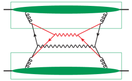
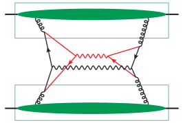
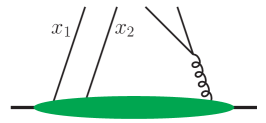
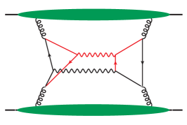
This points to another problem, namely that of double counting contributions between SPS and DPS. To see this, let us analyse the graph in figure 1a. Since the transverse boson momenta 𝒒1subscript𝒒1\boldsymbol{q}_{1} and 𝒒2subscript𝒒2\boldsymbol{q}_{2} are approximately back to back (up to effects from the transverse momenta of the incoming gluons) it is convenient to introduce the combination

𝒒𝒒\displaystyle\boldsymbol{q} =12(𝒒1𝒒2).absent12subscript𝒒1subscript𝒒2\displaystyle={\tfrac{1}{2}}(\boldsymbol{q}_{1}-\boldsymbol{q}_{2})\,. (10)

For qQimuch-less-than𝑞subscript𝑄𝑖q\ll Q_{i} the graph gives a leading contribution to dσ/dq2𝑑𝜎𝑑superscript𝑞2d\sigma/d{q}^{2} if the transverse quark momenta in the loops are all of order Qisubscript𝑄𝑖Q_{i}. This carries the quark lines far off shell, so that this contribution is naturally associated with SPS, with g+gV1V2𝑔𝑔subscript𝑉1subscript𝑉2g+g\to V_{1}V_{2} as the hard subprocess. A leading contribution is also obtained from the region where all transverse quark momenta are much smaller than Qisubscript𝑄𝑖Q_{i}. This region is naturally described as DPS, with two disconnected hard scattering processes qq¯V1𝑞¯𝑞subscript𝑉1q\bar{q}\to V_{1} and qq¯V2𝑞¯𝑞subscript𝑉2q\bar{q}\to V_{2} and double parton distributions with perturbative gqq¯𝑔𝑞¯𝑞g\to q\bar{q} splittings, indicated by the boxes in the graph. We denote this as a 1v1 (1 versus 1) contribution to DPS, emphasising its close relation to SPS.

A double counting problem for this graph obviously arises if one takes the loop integrals in the SPS cross section over all transverse quark momenta (including the DPS region), and likewise if one integrates the DPDs cross section over the full range of transverse positions, which is equivalent to integrating over all transverse momenta in the quark loops. The problem persists if one integrates the cross section over 𝒒𝒒\boldsymbol{q}.

Refer to caption
Refer to caption
Refer to caption
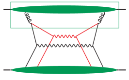
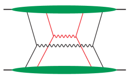
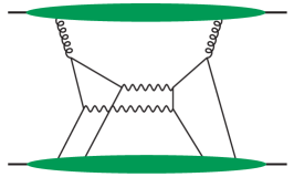
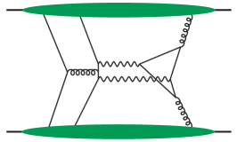
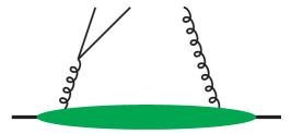
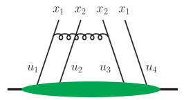
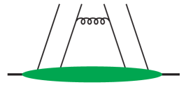
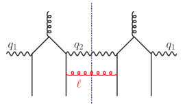
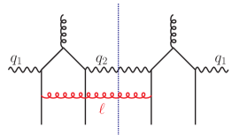
Figure 1: (a) A 1v1 contribution to DPS, with perturbative splitting DPDs for each proton (indicated by the boxes). (b) A 2v1 contribution to DPS, with a perturbative splitting DPD in only one proton (indicated by the box). (c) A 2v2 contribution to DPS. Here and in the following it is understood that partons emerging from the oval blobs are approximately collinear to their parent proton. A line for the final state cut across the blobs and the produced vector bosons (wavy lines) is not shown for simplicity.

Let us now turn to the graph in figure 1b and consider the cross section integrated over 𝒒1subscript𝒒1\boldsymbol{q}_{1} and 𝒒2subscript𝒒2\boldsymbol{q}_{2}. In the region of large qQisimilar-to𝑞subscript𝑄𝑖q\sim Q_{i}, the quark lines at the top of the graph have transverse momenta of order q𝑞q and are far off shell. The proper description of this region is in terms of a hard scattering qq¯+gV1V2𝑞¯𝑞𝑔subscript𝑉1subscript𝑉2q\bar{q}+g\to V_{1}V_{2}, convoluted with a collinear twist-two distribution (i.e. an ordinary PDF) at the top and a collinear twist-four distribution at the bottom of the graph. For brevity we refer to this as the “twist-four contribution” henceforth. In the region qQimuch-less-than𝑞subscript𝑄𝑖q\ll Q_{i}, the gqq¯𝑔𝑞¯𝑞g\to q\bar{q} splittings are near collinear and the approximations for DPS are appropriate. We call this the 2v1 contribution to DPS, recalling that there is a qq¯+g𝑞¯𝑞𝑔q\bar{q}+g subprocess in the graph. Both small and large q𝑞q give leading contributions to the integrated cross section, and in a naive calculation adding up the twist-four term and the DPS term has again a double counting problem, as well as divergences in each contribution. The naive DPS cross section has a logarithmic divergence at small y𝑦y, which is seen by inserting the 1/y21superscript𝑦21/y^{2} splitting behaviour of only one DPD in (2). In turn, the hard scattering cross section in the twist-four term contains a collinear divergence in the form of an integral behaving like dq2/q2𝑑superscript𝑞2superscript𝑞2dq^{2}/q^{2} at q0𝑞0q\to 0, as we will show in section 4.1.2.

Clearly, one needs a consistent scheme for computing the overall cross section, without double counting and without divergences in individual terms. An intuitive approach for evaluating DPS is to separate the “perturbative splitting” part of a DPD from its “intrinsic” nonperturbative part.222The intrinsic part of a DPD may be studied using quark models Chang:2012nw ; Rinaldi:2013vpa ; Rinaldi:2014ddl ; Rinaldi:2016jvu ; Rinaldi:2016mlk ; Broniowski:2013xba ; Broniowski:2016trx ; Kasemets:2016nio , at least in the valence region, or it may be related to the product of two PDFs if correlations between the two partons are neglected. This has been pursued independently by Blok et al. Blok:2011bu ; Blok:2013bpa and by Ryskin and Snigirev Ryskin:2011kk ; Ryskin:2012qx . Taking the intrinsic DPD for each proton, one obtains the 2v2 part of DPS, which does not contain any perturbative splitting and is shown in figure 1c. The splitting part of the DPD is explicitly computed in terms of a single parton distribution function (PDF) and a perturbative kernel. This is multiplied with an intrinsic DPD to compute the 2v1 term. Finally, the product of two splitting DPDs is used to compute the 1v1 contribution in the approach of Ryskin:2011kk ; Ryskin:2012qx , where an ultraviolet cutoff must be imposed to regulate the quadratic divergence we mentioned earlier. By contrast, the authors of Blok:2011bu ; Blok:2013bpa advocate to omit this term and replace it entirely with the SPS contribution to the cross section.

We are, however, not able to give a field theoretic definition of the “intrinsic” or “nonperturbative” part of a DPD. The consideration of Feynman graphs in the preceding arguments is instructive, but a satisfactory definition should only appeal to perturbation theory in regions where it is applicable. We regard a nonperturbative definition of DPDs as indispensable for a systematic theory approach, for instance for deriving evolution equations and other general properties.

The setup we propose in this work defines DPDs as operator matrix elements as described above, containing both splitting and intrinsic contributions. UV divergences in the DPS cross section are avoided by introducing (smooth or hard) cutoffs in the integrations over transverse distances. The double counting problems are treated within the subtraction formalism used in standard factorisation theorems, described in detail in sections 10.1 and 10.7 of Collins:2011zzd and briefly recalled in section 4 here. The subtraction terms that avoid double counting also remove the above mentioned collinear divergence in the twist-four term. A distinction between “splitting” and “intrinsic” contributions to a DPD will be made in the limit of small transverse distances, where it can be formulated in terms of an operator product expansion (see section 3.3), and when making a model ansatz for DPDs at large distances, which is of course necessary for phenomenology.

2.1 Contributions to the cross section: power behaviour and logarithms

In preparation for later sections, we now recall some results for the power behaviour of different contributions to the cross section, referring to section 2.4 of Diehl:2011yj for a derivation. We also recall which logarithms appear in the lowest order 1v1 and 1v2 graphs. As already stated, we take the process ppV1+V2+X𝑝𝑝subscript𝑉1subscript𝑉2𝑋pp\to V_{1}+V_{2}+X as a concrete example, but the discussion readily generalises to other cases.

The differential cross section dσ/(d2𝒒1d2𝒒2)𝑑𝜎superscript𝑑2subscript𝒒1superscript𝑑2subscript𝒒2d\sigma/(d^{2}\boldsymbol{q}_{1}\mskip 1.5mud^{2}\boldsymbol{q}_{2}) in the region qiQimuch-less-thansubscript𝑞𝑖subscript𝑄𝑖q_{i}\ll Q_{i} can be computed using TMD factorisation. Here and in the following we write Qisubscript𝑄𝑖Q_{i} to denote the generic size of Q1subscript𝑄1Q_{1} and Q2subscript𝑄2Q_{2}, and likewise for qisubscript𝑞𝑖q_{i}. The transverse momenta qisubscript𝑞𝑖q_{i} may be of nonperturbative size ΛΛ\Lambda or much larger. In the latter case, further simplifications are possible by expressing transverse momentum dependent distributions in terms of collinear ones Buffing:2016wip , but we shall not discuss this here. The leading power behaviour of the cross section is

dσd2𝒒1d2𝒒21Qi4qi2.similar-to𝑑𝜎superscript𝑑2subscript𝒒1superscript𝑑2subscript𝒒21superscriptsubscript𝑄𝑖4superscriptsubscript𝑞𝑖2\displaystyle\frac{d\sigma}{d^{2}\boldsymbol{q}_{1}\mskip 1.5mud^{2}\boldsymbol{q}_{2}}\sim\frac{1}{Q_{i}^{4}\,q_{i}^{2}}\,. (11)

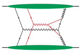
When qisubscript𝑞𝑖q_{i} goes to zero, it should be replaced by ΛΛ\Lambda. Three types of mechanisms contribute to the leading behaviour, namely DPS, SPS, and the interference between SPS and DPS. Corresponding graphs are shown in figures 1c, 2a and 2b, respectively.

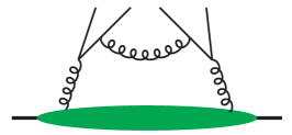
As discussed in the previous section, certain graphs contribute both to DPS and to SPS, depending on the kinematics of their internal lines. The 1v1 graph in figure 1 also has leading regions in which one of the loops is hard and the other is collinear. These regions contribute to the SPS/DPS interference, as shown in figure 2c. The double counting problem thus concerns both SPS, DPS and their interference. Note that the SPS graph in figure 2a contributes to the SPS/DPS interference but not to DPS.

Both the amplitude and its conjugate in the 1v1 graph contains a loop integral that behaves like d2𝒌/𝒌2superscript𝑑2𝒌superscript𝒌2d^{2}\boldsymbol{k}/\boldsymbol{k}^{2} in the region Λ,qikQimuch-less-thanΛsubscript𝑞𝑖𝑘much-less-thansubscript𝑄𝑖\Lambda,q_{i}\ll k\ll Q_{i}. When integrated over the full phase space, each loop thus builds up a so-called DPS logarithm, namely log(Qi/qi)subscript𝑄𝑖subscript𝑞𝑖\log(Q_{i}/q_{i}) when qi>Λsuperscriptsimilar-tosubscript𝑞𝑖Λq_{i}\raisebox{-4.0pt}{$\,\stackrel{{\scriptstyle\textstyle>}}{{\sim}}\,$}\Lambda and log(Qi/Λ)subscript𝑄𝑖Λ\log(Q_{i}/\Lambda) when qi<Λsuperscriptsimilar-tosubscript𝑞𝑖Λq_{i}\raisebox{-4.0pt}{$\,\stackrel{{\scriptstyle\textstyle<}}{{\sim}}\,$}\Lambda. Whether these logarithms reside in SPS, DPS or their interference depends on how exactly one handles the double counting problem. We come back to this issue in section 4.2.
Refer to caption
Refer to caption
Refer to caption
Figure 2: (a) A higher-order graph for SPS. The loop on the l.h.s. has a momentum region associated with DPS but the loop on the r.h.s. does not. (b) Interference between DPS in the amplitude and SPS in the complex conjugate amplitude. (c) 1v1 graph in the region where the quark loop on the left is collinear whilst the one on the right is hard. This corresponds to the region of SPS/DPS interference, with the boxes indicating DPDs with perturbative splitting for the parton pair in the amplitude.
Refer to caption
Refer to caption
Figure 3: (a) A graph with a twist-four distribution for one proton and a twist-two distribution for the other. (b) A graph with twist-three distributions for both protons.

Let us now turn to the cross section integrated over 𝒒1subscript𝒒1\boldsymbol{q}_{1} and 𝒒2subscript𝒒2\boldsymbol{q}_{2}, which can be described using collinear factorisation. The leading power behaviour of the cross section, σ1/Qi2similar-to𝜎1superscriptsubscript𝑄𝑖2\sigma\sim 1/Q_{i}^{2}, is given by the SPS mechanism alone. Several mechanisms contribute at the power suppressed level σΛ2/Qi4similar-to𝜎superscriptΛ2superscriptsubscript𝑄𝑖4\sigma\sim\Lambda^{2}/Q_{i}^{4}. These are

  1. 1.

    DPS, which is suppressed because it can only populate the region qiQimuch-less-thansubscript𝑞𝑖subscript𝑄𝑖q_{i}\ll Q_{i} rather than the full phase space up to qiQisimilar-tosubscript𝑞𝑖subscript𝑄𝑖q_{i}\sim Q_{i},

  2. 2.

    the interference between SPS and DPS, which is suppressed for the same reason,

  3. 3.

    hard scattering with a twist-four distribution for one proton and a twist-two distribution for the other. Example graphs are figure 3a, as well as figure 1b with the box removed.

  4. 4.

    hard scattering with twist-three distributions for both protons. An example graph is figure 3b.

The rationale for considering such contributions is that – whilst being power suppressed compared with SPS – they may be enhanced by higher parton luminosities at small momentum fractions x𝑥x, or by coupling constants in the relevant hard scattering subprocesses. Let us emphasise that a complete calculation of the cross section at the level of Λ2/Qi2superscriptΛ2superscriptsubscript𝑄𝑖2\Lambda^{2}/Q_{i}^{2} corrections would be a formidable task, and it is not even established whether factorisation (in particular the cancellation of Glauber gluons) holds at that level.

Notice that in collinear factorisation, the SPS/DPS interference term involves collinear twist three distributions for both protons, because the SPS mechanism forces the two partons in the interfering DPS amplitude to be at same transverse position (see section 2.4.1 in Diehl:2011yj ). In this sense, mechanism 2 in the above list may be regarded as a special case of mechanism 4, with a disconnected hard scattering in the amplitude or its conjugate (see figure 2b).

A full treatment of contributions with twist-three or twist-four distributions is beyond the scope of this paper. We remark however that twist-n𝑛n operators contain n𝑛n or less than n𝑛n parton fields, and that different operators are related by the equations of motion. For a detailed discussion we refer to Braun:2008ia ; Braun:2009vc ; Ji:2014eta . Twist-n𝑛n operators with n𝑛n parton fields were called “‘quasipartonic” in Bukhvostov:1985rn and involve only the “good” parton fields in the parlance of light-cone quantisation Jaffe:1996zw . These are exactly the fields appearing in the definitions of multiparton distributions, so that graphs with a double counting issue between higher-twist hard scattering and DPS (or the SPS/DPS interference) involve only quasipartonic operators.

The matrix elements of quasipartonic twist-three operators in an unpolarised target satisfy the important selection rule that the helicities carried by the parton lines must balance . This excludes three-gluon operators since three helicities ±1plus-or-minus1\pm 1 cannot add up to zero. For quark-antiquark-gluon operators it forces the quark and antiquark fields to have opposite chirality, i.e. one only has the operator combination q¯σ+jq¯𝑞superscript𝜎𝑗𝑞\bar{q}\sigma^{+j}q, where the transverse index j𝑗j is contracted with the polarisation index of the gluon. As for non-quasipartonic twist-three distributions in an unpolarised target, one finds that they are absent in the pure gluon sector Mulders:2000sh , whereas the corresponding quark-antiquark distributions are again chiral-odd Jaffe:1991ra . Since chiral-odd distributions cannot be generated by gluon ladder graphs, they lack the small x𝑥x enhancement that is one of the motivations to keep higher twist contributions in the cross section. We will therefore not discuss them further in this work. Note that corresponding selection rules do not hold for TMD correlators, where an imbalance in the helicities of the parton fields can be compensated by orbital angular momentum.

Let us finally recall the appearance of DPS logarithms in collinear factorisation. The 2v1 graph (figure 1b) has a behaviour dσ/dq21/q2similar-to𝑑𝜎𝑑superscript𝑞21superscript𝑞2d\sigma/dq^{2}\sim 1/q^{2} in the region ΛqQimuch-less-thanΛ𝑞much-less-thansubscript𝑄𝑖\Lambda\ll q\ll Q_{i}, which gives a log(Qi/Λ)subscript𝑄𝑖Λ\log(Q_{i}/\Lambda) when integrated over the full phase space. Depending on how the double counting between DPS and the twist-four mechanism is resolved, this logarithm can appear in different contributions to the cross section. We will discuss this in section 4.1.2.

3 Short-distance limit of DPDs

In this section, we analyse the behaviour of DPDs in the limit where the transverse distance between partons becomes small compared with the scale of nonperturbative interactions. In this region, the splitting of one parton into two becomes dominant. Generalising results in Diehl:2011yj we give expressions in D=42ϵ𝐷42italic-ϵD=4-2\epsilon dimensions, which are necessary in intermediate steps when constructing a factorisation formula for the cross section.

3.1 TMDs

A useful choice of position variables for describing the parton splitting mechanism is

𝒚±subscript𝒚plus-or-minus\displaystyle\boldsymbol{y}_{\pm} =𝒚±12(𝒛1𝒛2),absentplus-or-minus𝒚12subscript𝒛1subscript𝒛2\displaystyle=\boldsymbol{y}\pm{\tfrac{1}{2}}(\boldsymbol{z}_{1}-\boldsymbol{z}_{2})\,, 𝒁𝒁\displaystyle\boldsymbol{Z} =12(𝒛1+𝒛2)absent12subscript𝒛1subscript𝒛2\displaystyle={\tfrac{1}{2}}(\boldsymbol{z}_{1}+\boldsymbol{z}_{2}) (12)

with Fourier conjugate momenta 333The momentum 𝚫𝚫\boldsymbol{\Delta} is called 𝒓𝒓\boldsymbol{r} in Diehl:2011tt ; Diehl:2011yj .

𝒌±subscript𝒌plus-or-minus\displaystyle\boldsymbol{k}_{\pm} =12(𝒌1𝒌2±𝚫),absent12plus-or-minussubscript𝒌1subscript𝒌2𝚫\displaystyle={\tfrac{1}{2}}(\boldsymbol{k}_{1}-\boldsymbol{k}_{2}\pm\boldsymbol{\Delta})\,, 𝑲𝑲\displaystyle\boldsymbol{K} =𝒌1+𝒌2.absentsubscript𝒌1subscript𝒌2\displaystyle=\boldsymbol{k}_{1}+\boldsymbol{k}_{2}\,. (13)

The relation between DPDs in position and momentum space reads

F(xi,𝒚±,𝒁)𝐹subscript𝑥𝑖subscript𝒚plus-or-minus𝒁\displaystyle F(x_{i},\boldsymbol{y}_{\pm},\boldsymbol{Z})
=1(2π)22ϵd22ϵ𝑲d22ϵ𝒌+d22ϵ𝒌ei𝒁𝑲+i(𝒚+𝒌𝒚𝒌+)F(xi,𝒌±,𝑲)absent1superscript2𝜋22italic-ϵsuperscript𝑑22italic-ϵ𝑲superscript𝑑22italic-ϵsubscript𝒌superscript𝑑22italic-ϵsubscript𝒌superscript𝑒𝑖𝒁𝑲𝑖subscript𝒚subscript𝒌subscript𝒚subscript𝒌𝐹subscript𝑥𝑖subscript𝒌plus-or-minus𝑲\displaystyle\qquad=\frac{1}{(2\pi)^{2-2\epsilon}}\int d^{2-2\epsilon}\boldsymbol{K}\,d^{2-2\epsilon}\boldsymbol{k}_{+}\,d^{2-2\epsilon}\boldsymbol{k}_{-}\;e^{i\boldsymbol{Z}\boldsymbol{K}+i(\boldsymbol{y}_{+}\boldsymbol{k}_{-}-\boldsymbol{y}_{-}\boldsymbol{k}_{+})}\,F(x_{i},\boldsymbol{k}_{\pm},\boldsymbol{K}) (14)

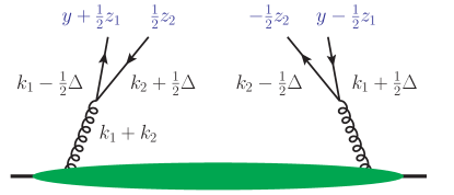
in D=42ϵ𝐷42italic-ϵD=4-2\epsilon dimensions. As seen in figure 4, one can identify 𝒚+subscript𝒚\boldsymbol{y}_{+} (𝒚subscript𝒚\boldsymbol{y}_{-}) as the transverse distance between the two partons on the left (right) hand side of the final state cut in the DPD. Correspondingly, the transverse momentum difference between the partons on the left (right) hand side of the cut is 𝒌subscript𝒌\boldsymbol{k}_{-} (𝒌+subscript𝒌\boldsymbol{k}_{+}). The splitting singularities of the DPDs thus occur at y±0subscript𝑦plus-or-minus0y_{\pm}\to 0 or k±subscript𝑘plus-or-minusk_{\pm}\to\infty.

Refer to caption
Figure 4: The perturbative splitting mechanism for a DPD, with momentum and position assignments. Here and in the following, the line for the final-state cut of the spectator partons is not shown for simplicity.

The perturbative splitting contribution Fspl,ptsubscript𝐹spl,ptF_{\text{spl,pt}} to transverse-momentum dependent DPDs in momentum space has been calculated at leading order in section 5.2.2 of Diehl:2011yj . Generalising these results to D=42ϵ𝐷42italic-ϵD=4-2\epsilon dimensions, we have

Fa1a2,spl,pt(xi,𝒌±,𝑲)subscript𝐹subscript𝑎1subscript𝑎2spl,ptsubscript𝑥𝑖subscript𝒌plus-or-minus𝑲\displaystyle F_{a_{1}a_{2},\mskip 1.5mu\text{spl,pt}}(x_{i},\boldsymbol{k}_{\pm},\boldsymbol{K}) =𝒌jk2𝒌+jk+2(2μ)2ϵπ12ϵabsentsuperscriptsubscript𝒌𝑗superscriptsubscript𝑘2superscriptsubscript𝒌superscript𝑗superscriptsubscript𝑘2superscript2𝜇2italic-ϵsuperscript𝜋12italic-ϵ\displaystyle=\frac{\boldsymbol{k}_{-}^{j}}{k_{-}^{2}}\,\frac{\boldsymbol{k}_{+}^{j^{\prime}}}{k_{+}^{2}}\,\frac{(2\mu)^{2\epsilon}}{\pi^{1-2\epsilon}}\,
×[fa0(x1+x2,𝑲)x1+x2αs2πTa0a1a2jj(x1x1+x2,ϵ)+],absentdelimited-[]subscript𝑓subscript𝑎0subscript𝑥1subscript𝑥2𝑲subscript𝑥1subscript𝑥2subscript𝛼𝑠2𝜋subscriptsuperscript𝑇𝑗superscript𝑗subscript𝑎0subscript𝑎1subscript𝑎2subscript𝑥1subscript𝑥1subscript𝑥2italic-ϵ\displaystyle\quad\times\biggl{[}\frac{f_{a_{0}}(x_{1}+x_{2},\boldsymbol{K})}{x_{1}+x_{2}}\,\frac{\alpha_{s}}{2\pi}\,T^{jj^{\prime}}_{a_{0}\to a_{1}a_{2}}\biggl{(}\frac{x_{1}}{x_{1}+x_{2}},\epsilon\biggr{)}+\ldots\,\biggr{]}\,, (15)

where j𝑗j, jsuperscript𝑗j^{\prime} are transverse Lorentz indices and fa0(x1+x2,𝑲)subscript𝑓subscript𝑎0subscript𝑥1subscript𝑥2𝑲f_{a_{0}}(x_{1}+x_{2},\boldsymbol{K}) is an unpolarised single-parton TMD.444Compared with section 5.2 of Diehl:2011yj , the kernel Tjjsuperscript𝑇𝑗superscript𝑗T^{jj^{\prime}} used here has the opposite order of indices jj𝑗superscript𝑗jj^{\prime} and includes a colour factor, e.g. TF=1/2subscript𝑇𝐹12T_{F}=1/2 for the colour singlet distribution Fgqq¯1superscriptsubscript𝐹𝑔𝑞¯𝑞1{}^{1}F_{g\to q\bar{q}}. The ellipsis denotes a term that involves a TMD for polarised partons in an unpolarised proton and depends on 𝑲𝑲\boldsymbol{K} but not on 𝒌±subscript𝒌plus-or-minus\boldsymbol{k}_{\pm}. In position space we then get

Fa1a2,spl,pt(xi,𝒚±,𝒁)subscript𝐹subscript𝑎1subscript𝑎2spl,ptsubscript𝑥𝑖subscript𝒚plus-or-minus𝒁\displaystyle F_{a_{1}a_{2},\mskip 1.5mu\text{spl,pt}}(x_{i},\boldsymbol{y}_{\pm},\boldsymbol{Z}) =𝒚+jy+22ϵ𝒚jy22ϵμ2ϵΓ2(1ϵ)π12ϵabsentsuperscriptsubscript𝒚𝑗superscriptsubscript𝑦22italic-ϵsuperscriptsubscript𝒚superscript𝑗superscriptsubscript𝑦22italic-ϵsuperscript𝜇2italic-ϵsuperscriptΓ21italic-ϵsuperscript𝜋12italic-ϵ\displaystyle=\frac{\boldsymbol{y}_{+}^{j}}{y_{+}^{2-2\epsilon}}\,\frac{\boldsymbol{y}_{-}^{j^{\prime}}}{y_{-}^{2-2\epsilon}}\,\mu^{2\epsilon}\,\frac{\Gamma^{2}(1-\epsilon)}{\pi^{1-2\epsilon}}\,
×[fa0(x1+x2,𝒁)x1+x2αs2πTa0a1a2jj(x1x1+x2,ϵ)+]absentdelimited-[]subscript𝑓subscript𝑎0subscript𝑥1subscript𝑥2𝒁subscript𝑥1subscript𝑥2subscript𝛼𝑠2𝜋subscriptsuperscript𝑇𝑗superscript𝑗subscript𝑎0subscript𝑎1subscript𝑎2subscript𝑥1subscript𝑥1subscript𝑥2italic-ϵ\displaystyle\quad\times\biggl{[}\frac{f_{a_{0}}(x_{1}+x_{2},\boldsymbol{Z})}{x_{1}+x_{2}}\,\frac{\alpha_{s}}{2\pi}\,T^{jj^{\prime}}_{a_{0}\to a_{1}a_{2}}\biggl{(}\frac{x_{1}}{x_{1}+x_{2}},\epsilon\biggr{)}+\ldots\,\biggr{]} (16)

using the Fourier integral (166), where the term denoted by an ellipsis depends on 𝒁𝒁\boldsymbol{Z} but not on 𝒚±subscript𝒚plus-or-minus\boldsymbol{y}_{\pm}. It is understood that for transverse quark or linear gluon polarisation, both Fa1a2subscript𝐹subscript𝑎1subscript𝑎2F_{a_{1}a_{2}} and the kernel T𝑇T carry additional transverse Lorentz indices. fa0(x1+x2,𝒁)subscript𝑓subscript𝑎0subscript𝑥1subscript𝑥2𝒁f_{a_{0}}(x_{1}+x_{2},\boldsymbol{Z}) is the Fourier transform of fa0(x1+x2,𝑲)subscript𝑓subscript𝑎0subscript𝑥1subscript𝑥2𝑲f_{a_{0}}(x_{1}+x_{2},\boldsymbol{K}). The form (3.1) gives the leading behaviour of the DPD for large k±Λmuch-greater-thansubscript𝑘plus-or-minusΛk_{\pm}\gg\Lambda, and correspondingly (3.1) gives the leading behaviour for y±1/Λmuch-less-thansubscript𝑦plus-or-minus1Λy_{\pm}\ll 1/\Lambda.

If one inserts these results into the cross section formula and sets D=4𝐷4D=4, logarithmic divergences appear at y+=0subscript𝑦0y_{+}=0 and y=0subscript𝑦0y_{-}=0. To make them explicit we transform variables to

d2𝒚d2𝒛1d2𝒛2ei(𝒒1𝒛1+𝒒2𝒛2)superscript𝑑2𝒚superscript𝑑2subscript𝒛1superscript𝑑2subscript𝒛2superscript𝑒𝑖subscript𝒒1subscript𝒛1subscript𝒒2subscript𝒛2\displaystyle\int d^{2}\boldsymbol{y}\,d^{2}\boldsymbol{z}_{1}\,d^{2}\boldsymbol{z}_{2}\;e^{-i(\boldsymbol{q}_{1}\boldsymbol{z}_{1}+\boldsymbol{q}_{2}\boldsymbol{z}_{2})} =d2𝒁d2𝒚+d2𝒚ei(𝒒1+𝒒2)𝒁ei𝒒(𝒚+𝒚)absentsuperscript𝑑2𝒁superscript𝑑2subscript𝒚superscript𝑑2subscript𝒚superscript𝑒𝑖subscript𝒒1subscript𝒒2𝒁superscript𝑒𝑖𝒒subscript𝒚subscript𝒚\displaystyle=\int d^{2}\boldsymbol{Z}\,d^{2}\boldsymbol{y}_{+}\,d^{2}\boldsymbol{y}_{-}\;e^{-i(\boldsymbol{q}_{1}+\boldsymbol{q}_{2})\boldsymbol{Z}}e^{-i\boldsymbol{q}(\boldsymbol{y}_{+}-\boldsymbol{y}_{-})} (17)

with 𝒒𝒒\boldsymbol{q} defined in (10). Performing the angular integration in

1πd2𝒚e±i𝒒𝒚𝒚j𝒚jy41𝜋superscript𝑑2𝒚superscript𝑒plus-or-minus𝑖𝒒𝒚superscript𝒚𝑗superscript𝒚superscript𝑗superscript𝑦4\displaystyle\frac{1}{\pi}\int d^{2}\boldsymbol{y}\;e^{\mskip 1.5mu\pm i\boldsymbol{q}\boldsymbol{y}}\,\frac{\boldsymbol{y}^{j}\boldsymbol{y}^{j^{\prime}}}{y^{4}} =δjjdyyJ0(yq)+(δjj2𝒒j𝒒jq2)dyyJ2(yq),absentsuperscript𝛿𝑗superscript𝑗𝑑𝑦𝑦subscript𝐽0𝑦𝑞superscript𝛿𝑗superscript𝑗2superscript𝒒𝑗superscript𝒒superscript𝑗superscript𝑞2𝑑𝑦𝑦subscript𝐽2𝑦𝑞\displaystyle=\delta^{jj^{\prime}}\!\int\frac{dy}{y}\,J_{0}(yq)+\biggl{(}\delta^{jj^{\prime}}-\frac{2\boldsymbol{q}^{j}\boldsymbol{q}^{j^{\prime}}}{q^{2}}\biggr{)}\int\frac{dy}{y}\,J_{2}(yq)\,, (18)

where 𝒚𝒚\boldsymbol{y} stands for 𝒚+subscript𝒚\boldsymbol{y}_{+} or 𝒚subscript𝒚\boldsymbol{y}_{-}, we see that the integral with J0subscript𝐽0J_{0} is divergent at y=0𝑦0y=0. Given the range of validity of (3.1) one should impose y1/Λmuch-less-than𝑦1Λy\ll 1/\Lambda in (18), although the integrals are finite for y𝑦y\to\infty due to the oscillations of the Bessel functions.

The perturbative splitting contribution to DPDs at higher order in αssubscript𝛼𝑠\alpha_{s} involves graphs with additional partons radiated into the final state as shown in figure 5a, as well as virtual corrections. It is natural to expect that it will again be singular at y±=0subscript𝑦plus-or-minus0y_{\pm}=0. A calculation of this contribution is outside the scope of the present work, so that we will limit our analysis of TMD factorisation to perturbative splitting at LO.

To compute the DPD cross section, we must also consider the case where only one of the distances y+subscript𝑦y_{+} or ysubscript𝑦y_{-} is small, whereas the other one remains large. In this case, one has a perturbative splitting only on one side of the final-state cut, as illustrated in figure 5b. We will not discuss the detailed expression of the DPD in this regime, but give its general structure. Setting D=4𝐷4D=4 for simplicity, we have

Fα1α2,y0(xi,𝒚±,𝒁)subscript𝐹subscript𝛼1subscript𝛼2subscript𝑦0subscript𝑥𝑖subscript𝒚plus-or-minus𝒁\displaystyle F_{\alpha_{1}\alpha_{2},\mskip 1.5muy_{-}\to 0}(x_{i},\boldsymbol{y}_{\pm},\boldsymbol{Z}) =𝒚jy2[Uα0α1α2j(xi)]Dα1α2|α0(xi,𝒚+,𝒁),absentsuperscriptsubscript𝒚superscript𝑗superscriptsubscript𝑦2superscriptdelimited-[]subscriptsuperscript𝑈superscript𝑗subscript𝛼0subscript𝛼1subscript𝛼2subscript𝑥𝑖subscript𝐷conditionalsubscript𝛼1subscript𝛼2subscript𝛼0subscript𝑥𝑖subscript𝒚𝒁\displaystyle=\frac{\boldsymbol{y}_{-}^{j^{\prime}}}{y_{-}^{2}}\,\bigl{[}U^{j^{\prime}}_{\alpha_{0}\to\alpha_{1}\alpha_{2}}(x_{i})\bigr{]}^{*}\,D_{\alpha_{1}\alpha_{2}|\alpha_{0}}(x_{i},\boldsymbol{y}_{+},\boldsymbol{Z})\,, (19)

were Uα0α1α2subscript𝑈subscript𝛼0subscript𝛼1subscript𝛼2U_{\alpha_{0}\to\alpha_{1}\alpha_{2}} is a kernel for the splitting α0α1α2subscript𝛼0subscript𝛼1subscript𝛼2\alpha_{0}\to\alpha_{1}\alpha_{2} in the amplitude (hence its complex conjugate appears in (19)). Dα1α2|α0subscript𝐷conditionalsubscript𝛼1subscript𝛼2subscript𝛼0D_{\alpha_{1}\alpha_{2}|\alpha_{0}} is the position space version of a transverse-momentum dependent twist-three distribution, constructed from the hadronic matrix element

p|ϕ0(12Z)ϕ2(12(Zy+))ϕ1(12(Z+y+))|pquantum-operator-product𝑝subscriptitalic-ϕ012𝑍subscriptitalic-ϕ212𝑍subscript𝑦subscriptitalic-ϕ112𝑍subscript𝑦𝑝\displaystyle\bigl{\langle}p\mskip 1.5mu\big{|}\phi_{0}\bigl{(}-{\tfrac{1}{2}}Z\bigr{)}\,\phi_{2}\bigl{(}{\tfrac{1}{2}}(Z-y_{+})\bigr{)}\,\phi_{1}\bigl{(}{\tfrac{1}{2}}(Z+y_{+})\bigr{)}\big{|}\mskip 1.5mup\bigr{\rangle}
=p|ϕ0(12(yZ))ϕ2(12z2)ϕ1(y+12z1)|p,absentquantum-operator-product𝑝subscriptitalic-ϕ012𝑦𝑍subscriptitalic-ϕ212subscript𝑧2subscriptitalic-ϕ1𝑦12subscript𝑧1𝑝\displaystyle\qquad\quad=\bigl{\langle}p\mskip 1.5mu\big{|}\phi_{0}\bigl{(}{\tfrac{1}{2}}(y-Z)\bigr{)}\,\phi_{2}\bigl{(}{\tfrac{1}{2}}z_{2}\bigr{)}\,\phi_{1}\bigl{(}y+{\tfrac{1}{2}}z_{1}\bigr{)}\big{|}\mskip 1.5mup\bigr{\rangle}\,, (20)

where ϕisubscriptitalic-ϕ𝑖\phi_{i} is a “good” field for parton αisubscript𝛼𝑖\alpha_{i} (cf. section 2.1). Distributions Dα0|α1α2(xi,𝒚,𝒁)subscript𝐷conditionalsubscript𝛼0subscript𝛼1subscript𝛼2subscript𝑥𝑖subscript𝒚𝒁D_{\alpha_{0}|\alpha_{1}\alpha_{2}}(x_{i},\boldsymbol{y}_{-},\boldsymbol{Z}) where α0subscript𝛼0\alpha_{0} belongs to the amplitude and α1,α2subscript𝛼1subscript𝛼2\alpha_{1},\alpha_{2} to the complex conjugate amplitude are defined in analogy. In the second step of (3.1) we have used translation invariance and shifted the parton fields to the same position as in the corresponding DPD (see figure 4). The labels αisubscript𝛼𝑖\alpha_{i} denote the parton species; it is understood that in (19) and the following equations parton helicities are taken fixed on the l.h.s. and must be appropriately summed over on the r.h.s. Note the difference between this notation and the labels aisubscript𝑎𝑖a_{i}, which denote parton species and polarisation (none, longitudinal, transverse or linear) and thus refer to a pair of parton legs. The notation with aisubscript𝑎𝑖a_{i} is hence not suitable for distributions with three parton fields.
Refer to caption
Refer to caption
Refer to caption
Figure 5: (a) A higher order contribution to the splitting part of a DPD. (b) Graph for a DPD with perturbative splitting only to the right of the final-state cut. The blob denotes a distribution Dα1α2|α0subscript𝐷conditionalsubscript𝛼1subscript𝛼2subscript𝛼0D_{\alpha_{1}\alpha_{2}|\alpha_{0}}. (c) Graph for perturbative splitting in the distribution Dα1α2|α0subscript𝐷conditionalsubscript𝛼1subscript𝛼2subscript𝛼0D_{\alpha_{1}\alpha_{2}|\alpha_{0}}.

If y+subscript𝑦y_{+} is small, then Dα1α2|α0(xi,𝒚+,𝒁)subscript𝐷conditionalsubscript𝛼1subscript𝛼2subscript𝛼0subscript𝑥𝑖subscript𝒚𝒁D_{\alpha_{1}\alpha_{2}|\alpha_{0}}(x_{i},\boldsymbol{y}_{+},\boldsymbol{Z}) itself can be generated by perturbative splitting, as shown in figure 5c. We have

Dα1α2|α0,y+0(xi,𝒚+,𝒁)subscript𝐷conditionalsubscript𝛼1subscript𝛼2subscript𝛼0subscript𝑦0subscript𝑥𝑖subscript𝒚𝒁\displaystyle D_{\alpha_{1}\alpha_{2}|\alpha_{0},\mskip 1.5muy_{+}\to 0}(x_{i},\boldsymbol{y}_{+},\boldsymbol{Z}) =𝒚+jy+2Uα0α1α2j(xi)fα0(x1+x2,𝒁).absentsuperscriptsubscript𝒚𝑗superscriptsubscript𝑦2subscriptsuperscript𝑈𝑗subscript𝛼0subscript𝛼1subscript𝛼2subscript𝑥𝑖subscript𝑓subscript𝛼0subscript𝑥1subscript𝑥2𝒁\displaystyle=\frac{\boldsymbol{y}_{+}^{j}}{y_{+}^{2}}\,U^{j}_{\alpha_{0}\to\alpha_{1}\alpha_{2}}(x_{i})\,f_{\alpha_{0}}(x_{1}+x_{2},\boldsymbol{Z})\,. (21)

Notice that a quark and antiquark produced by perturbative splitting have opposite helicities, so that the corresponding quark-antiquark operator ϕ2ϕ1subscriptitalic-ϕ2subscriptitalic-ϕ1\phi_{2}\,\phi_{1} in Dqq¯|gsubscript𝐷conditional𝑞¯𝑞𝑔D_{q\bar{q}\mskip 1.5mu|g} must be chiral-even. Inserting (21) into (19) we obtain

Fα1α2,y±0(xi,𝒚±,𝒁)subscript𝐹subscript𝛼1subscript𝛼2subscript𝑦plus-or-minus0subscript𝑥𝑖subscript𝒚plus-or-minus𝒁\displaystyle F_{\alpha_{1}\alpha_{2},\mskip 1.5muy_{\pm}\to 0}(x_{i},\boldsymbol{y}_{\pm},\boldsymbol{Z})
=𝒚+jy+2𝒚jy2Uα0α1α2j(xi)[Uα0α1α2j(xi)]fα0(x1+x2,𝒁).absentsuperscriptsubscript𝒚𝑗superscriptsubscript𝑦2superscriptsubscript𝒚superscript𝑗superscriptsubscript𝑦2subscriptsuperscript𝑈𝑗subscript𝛼0subscript𝛼1subscript𝛼2subscript𝑥𝑖superscriptdelimited-[]subscriptsuperscript𝑈superscript𝑗subscript𝛼0subscript𝛼1subscript𝛼2subscript𝑥𝑖subscript𝑓subscript𝛼0subscript𝑥1subscript𝑥2𝒁\displaystyle\quad=\frac{\boldsymbol{y}_{+}^{j}}{y_{+}^{2}}\,\frac{\boldsymbol{y}_{-}^{j^{\prime}}}{y_{-}^{2}}\,U^{j}_{\alpha_{0}\to\alpha_{1}\alpha_{2}}(x_{i})\,\bigl{[}U^{j^{\prime}}_{\alpha_{0}\to\alpha_{1}\alpha_{2}}(x_{i})\bigr{]}^{*}\,f_{\alpha_{0}}(x_{1}+x_{2},\boldsymbol{Z})\,. (22)

Taking appropriate linear combinations of parton helicities, we recover the form of Fa1a2,spl,ptsubscript𝐹subscript𝑎1subscript𝑎2spl,ptF_{a_{1}a_{2},\mskip 1.5mu\text{spl,pt}} in (3.1) at ϵ=0italic-ϵ0\epsilon=0.

3.2 Collinear DPDs: splitting contribution

We now turn to collinear DPDs, i.e. to the case where 𝒛1=𝒛2=𝟎subscript𝒛1subscript𝒛20\boldsymbol{z}_{1}=\boldsymbol{z}_{2}=\boldsymbol{0}. Let us first consider distributions for two unpolarised or two longitudinally polarised partons, so that the DPDs do not carry any transverse Lorentz indices. The lowest order splitting has been computed in Diehl:2011yj . For 42ϵ42italic-ϵ4-2\epsilon dimensions, one finds the general form

Fa1a2,spl,pt(x1,x2,𝒚;μ)subscript𝐹subscript𝑎1subscript𝑎2spl,ptsubscript𝑥1subscript𝑥2𝒚𝜇\displaystyle F_{a_{1}a_{2},\mskip 1.5mu\text{spl,pt}}(x_{1},x_{2},\boldsymbol{y};\mu)
=μ2ϵy24ϵΓ2(1ϵ)π12ϵfa0(x1+x2;μ)x1+x2αs(μ)2πPa0a1a2(x1x1+x2,ϵ).absentsuperscript𝜇2italic-ϵsuperscript𝑦24italic-ϵsuperscriptΓ21italic-ϵsuperscript𝜋12italic-ϵsubscript𝑓subscript𝑎0subscript𝑥1subscript𝑥2𝜇subscript𝑥1subscript𝑥2subscript𝛼𝑠𝜇2𝜋subscript𝑃subscript𝑎0subscript𝑎1subscript𝑎2subscript𝑥1subscript𝑥1subscript𝑥2italic-ϵ\displaystyle\quad=\frac{\mu^{2\epsilon}}{y^{2-4\epsilon}}\,\frac{\Gamma^{2}(1-\epsilon)}{\pi^{1-2\epsilon}}\,\frac{f_{a_{0}}(x_{1}+x_{2};\mu)}{x_{1}+x_{2}}\,\frac{\alpha_{s}(\mu)}{2\pi}\,P_{a_{0}\to a_{1}a_{2}}\biggl{(}\frac{x_{1}}{x_{1}+x_{2}},\epsilon\biggr{)}\,. (23)

The kernel for the splitting gqq¯𝑔𝑞¯𝑞g\to q\bar{q} reads for instance

Pgqq¯(u,ϵ)subscript𝑃𝑔𝑞¯𝑞𝑢italic-ϵ\displaystyle P_{g\to q\bar{q}\,}(u,\epsilon) =f2u2+(1u)2ϵ1ϵabsent𝑓2superscript𝑢2superscript1𝑢2italic-ϵ1italic-ϵ\displaystyle=\frac{f}{2}\,\frac{u^{2}+(1-u)^{2}-\epsilon}{1-\epsilon} (24)

with a factor f=1𝑓1f=1 for the colour singlet and f=1/N21𝑓1superscript𝑁21f=-1/\sqrt{N^{2}-1} for the colour octet DPD. In terms of the kernel in (3.1) we have Tgqq¯jj=δjjPgqq¯subscriptsuperscript𝑇𝑗superscript𝑗𝑔𝑞¯𝑞subscriptsuperscript𝛿𝑗superscript𝑗absentsubscript𝑃𝑔𝑞¯𝑞T^{jj^{\prime}}_{g\to q\bar{q}}=\delta^{jj^{\prime}}_{\phantom{q}}P_{g\to q\bar{q}}. We recognise in Pgqq¯(u,0)subscript𝑃𝑔𝑞¯𝑞𝑢0P_{g\to q\bar{q}}(u,0) the usual DGLAP splitting kernel without the terms proportional to δ(1u)𝛿1𝑢\delta(1-u).

Going beyond leading order, one can deduce the general form of the perturbative splitting contribution using dimensional analysis and boost invariance. For colour singlet distributions one finds

Fa1a2,spl,pt1(x1,x2,𝒚;μ)superscriptsubscript𝐹subscript𝑎1subscript𝑎2spl,pt1subscript𝑥1subscript𝑥2𝒚𝜇\displaystyle{}^{1}F_{a_{1}a_{2},\mskip 1.5mu\text{spl,pt}}(x_{1},x_{2},\boldsymbol{y};\mu)
=1π1ϵy22ϵa0x1+x21dvvfa0(v;μ)vVa0a1a2(x1v,x2v,αs(μ),yμ,ϵ)absent1superscript𝜋1italic-ϵsuperscript𝑦22italic-ϵsubscriptsubscript𝑎0superscriptsubscriptsubscript𝑥1subscript𝑥21𝑑𝑣𝑣subscript𝑓subscript𝑎0𝑣𝜇𝑣subscript𝑉subscript𝑎0subscript𝑎1subscript𝑎2subscript𝑥1𝑣subscript𝑥2𝑣subscript𝛼𝑠𝜇𝑦𝜇italic-ϵ\displaystyle\qquad=\frac{1}{\pi^{1-\epsilon}\,y^{2-2\epsilon}}\,\sum_{a_{0}}\int\limits_{x_{1}+x_{2}}^{1}\frac{dv}{v}\,\frac{f_{a_{0}}(v;\mu)}{v}\,V_{a_{0}\to a_{1}a_{2}}\biggl{(}\frac{x_{1}}{v},\frac{x_{2}}{v},\alpha_{s}(\mu),y\mu,\epsilon\biggr{)} (25)

in D=42ϵ𝐷42italic-ϵD=4-2\epsilon dimensions. The convolution integral over v𝑣v is familiar from factorisation formulae for hard scattering processes. Both f𝑓f and V𝑉V on the right-hand side are understood to include all necessary subtractions, so that they are finite at ϵ=0italic-ϵ0\epsilon=0. The splitting kernel V𝑉V is a double series

Va0a1a2(v1,v2,αs,yμ,ϵ)subscript𝑉subscript𝑎0subscript𝑎1subscript𝑎2subscript𝑣1subscript𝑣2subscript𝛼𝑠𝑦𝜇italic-ϵ\displaystyle V_{a_{0}\to a_{1}a_{2}}(v_{1},v_{2},\alpha_{s},y\mu,\epsilon) =n=1αsnm=1n(yμ)2ϵmVa0a1a2(n,m)(v1,v2,ϵ).absentsuperscriptsubscript𝑛1superscriptsubscript𝛼𝑠𝑛superscriptsubscript𝑚1𝑛superscript𝑦𝜇2italic-ϵ𝑚subscriptsuperscript𝑉𝑛𝑚subscript𝑎0subscript𝑎1subscript𝑎2subscript𝑣1subscript𝑣2italic-ϵ\displaystyle=\sum_{n=1}^{\infty}\alpha_{s}^{n}\sum_{m=1}^{n}(y\mu)^{2\epsilon m}\,V^{(n,m)}_{a_{0}\to a_{1}a_{2}}(v_{1},v_{2},\epsilon)\,. (26)

The μ𝜇\mu (and thus on dimensional grounds the y𝑦y) dependence of V𝑉V follows from the fact that the mass parameter of dimensional regularisation appears in graphs only via μ2ϵαs(μ)superscript𝜇2italic-ϵsubscript𝛼𝑠𝜇\mu^{2\epsilon}\alpha_{s}(\mu); terms with n>m𝑛𝑚n>m in (26) are due to the subtractions of ultraviolet or collinear divergences. At lowest order, the hard splitting graphs are disconnected (with no partons across the final state cut), so that V(1,1)(v1,v2,ϵ)=δ(1v1v2)V(1)(v1,ϵ)superscript𝑉11subscript𝑣1subscript𝑣2italic-ϵ𝛿1subscript𝑣1subscript𝑣2superscript𝑉1subscript𝑣1italic-ϵV^{(1,1)}(v_{1},v_{2},\epsilon)=\delta(1-v_{1}-v_{2})\,V^{(1)}(v_{1},\epsilon). Inserted into (3.2) this gives a form consistent with (3.2). Using that at order αsnsuperscriptsubscript𝛼𝑠𝑛\alpha_{s}^{n} the poles of highest order are 1/ϵn11superscriptitalic-ϵ𝑛11/\epsilon^{n-1}, we find

Va0a1a2(v1,v2,αs,yμ,0)subscript𝑉subscript𝑎0subscript𝑎1subscript𝑎2subscript𝑣1subscript𝑣2subscript𝛼𝑠𝑦𝜇0\displaystyle V_{a_{0}\to a_{1}a_{2}}(v_{1},v_{2},\alpha_{s},y\mu,0) =n=1αsnm=0n1logm(yμ)Va0a1a2[n,m](v1,v2).absentsuperscriptsubscript𝑛1superscriptsubscript𝛼𝑠𝑛superscriptsubscript𝑚0𝑛1superscript𝑚𝑦𝜇subscriptsuperscript𝑉𝑛𝑚subscript𝑎0subscript𝑎1subscript𝑎2subscript𝑣1subscript𝑣2\displaystyle=\sum_{n=1}^{\infty}\alpha_{s}^{n}\sum_{m=0}^{n-1}\log^{m}(y\mu)\,V^{[n,m]}_{a_{0}\to a_{1}a_{2}}(v_{1},v_{2})\,. (27)

in the physical limit ϵ=0italic-ϵ0\epsilon=0.

For colour nonsinglet DPDs one must regulate rapidity divergences, which complicates the preceding result. Taking e.g. Wilson lines along non-lightlike paths introduces additional vectors and changes the analysis of boost properties of the kernel. We will not pursue this issue here.

DPDs with transverse quark or linear gluon polarisation carry transverse Lorentz indices. Their perturbative splitting expressions thus have a tensor structure containing additional factors of 𝒚j/ysuperscript𝒚𝑗𝑦\boldsymbol{y}^{j}/y compared with the formulae above. At leading order one readily finds from (3.1) and the appropriate splitting kernels that the factor 1/y24ϵ1superscript𝑦24italic-ϵ1/y^{2-4\epsilon} in (3.2) is to be replaced with 𝒚j𝒚j/y44ϵsuperscript𝒚𝑗superscript𝒚superscript𝑗superscript𝑦44italic-ϵ\boldsymbol{y}^{j}\boldsymbol{y}^{j^{\prime}}/y^{4-4\epsilon} times a tensor constructed only from Kronecker deltas.

3.3 Collinear DPDs: all contributions

Let us now study the small y𝑦y behaviour of collinear DPDs in more general terms. We start by writing the relation between unrenormalised DPDs in position and momentum space as

(2π)D2F(𝒚)superscript2𝜋𝐷2𝐹𝒚\displaystyle(2\pi)^{D-2}F(\boldsymbol{y}) =dD2𝚫F(𝚫)+dD2𝚫[ei𝒚𝚫1]F(𝚫),absentsuperscript𝑑𝐷2𝚫𝐹𝚫superscript𝑑𝐷2𝚫delimited-[]superscript𝑒𝑖𝒚𝚫1𝐹𝚫\displaystyle=\int d^{D-2}\boldsymbol{\Delta}\;F(\boldsymbol{\Delta})+\int d^{D-2}\boldsymbol{\Delta}\;[e^{-i\boldsymbol{y}\boldsymbol{\Delta}}-1]\,F(\boldsymbol{\Delta})\,, (28)

omitting all arguments other than 𝒚𝒚\boldsymbol{y} and 𝚫𝚫\boldsymbol{\Delta}. The first term on the r.h.s. is a collinear twist-four distribution, independent of any transverse variable. For small y𝑦y, the second term is dominated by large 𝚫𝚫\boldsymbol{\Delta}, so that one can replace F(𝚫)𝐹𝚫F(\boldsymbol{\Delta}) by its approximation for large ΔΔ\Delta, following the power counting analysis of section 5.2 in Diehl:2011yj . This leads us to write

Fy0(𝒚)subscript𝐹𝑦0𝒚\displaystyle F_{y\to 0}(\boldsymbol{y}) =Fspl,pt(𝒚)+Ftw3,pt(𝒚)+Fint,pt(𝒚),absentsubscript𝐹spl,pt𝒚subscript𝐹tw3,pt𝒚subscript𝐹int,pt𝒚\displaystyle=F_{\text{spl,pt}}(\boldsymbol{y})+F_{\text{tw3,pt}}(\boldsymbol{y})+F_{\text{int,pt}}(\boldsymbol{y})\,, (29)

where the three terms on the r.h.s. will be described shortly. In D=4𝐷4D=4 dimensions, they respectively go like y2superscript𝑦2y^{-2}, y1superscript𝑦1y^{-1} and y0superscript𝑦0y^{0}, up to logarithmic corrections. Further terms from the perturbative expansion of F(𝚫)𝐹𝚫F(\boldsymbol{\Delta}) give contributions to F(𝒚)𝐹𝒚F(\boldsymbol{y}) that vanish like y𝑦y or faster.

One may also derive the expansion (29) from the operator product expansion, without taking recourse to the transverse momentum representation (28). In the definition of collinear DPDs one has a product 𝒪2(0,z2)𝒪1(y,z1)subscript𝒪20subscript𝑧2subscript𝒪1𝑦subscript𝑧1\mathcal{O}_{2}(0,z_{2})\,\mathcal{O}_{1}(y,z_{1}) of operators with 𝒛1=𝒛2=𝟎subscript𝒛1subscript𝒛20\boldsymbol{z}_{1}=\boldsymbol{z}_{2}=\boldsymbol{0} but nonzero 𝒚𝒚\boldsymbol{y}. This can be expanded around 𝒚=𝟎𝒚0\boldsymbol{y}=\boldsymbol{0} in terms of light-ray operators where all fields are at transverse position 𝟎0\boldsymbol{0}. These operators have twist 2, 3, 4 for the first, second and third term in (29), respectively.

The spitting contribution Fspl,ptsubscript𝐹spl,ptF_{\text{spl,pt}} is given by graphs as in figures 4 and 5a and has already been discussed in the previous subsection. The term Ftw3,ptsubscript𝐹tw3,ptF_{\text{tw3,pt}} originates from two types of graphs. The first type involves a single perturbative splitting and a quasipartonic collinear twist-three distribution as shown in figure 5b. The second type has two splittings as in figure 4 and a twist-three distribution with one “good” and one “bad” parton field. Given the helicity constraints discussed in section 2.1, collinear twist-three distributions in an unpolarised proton involve a quark and antiquark with opposite chirality (and possibly an extra gluon). As announced earlier, we discard twist-three terms in the following, since they are expected to become unimportant at small momentum fractions x1,x2subscript𝑥1subscript𝑥2x_{1},x_{2}.

Refer to caption
Refer to caption
Refer to caption
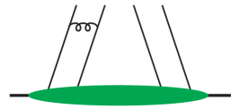
Figure 6: Graphs for the short-distance behaviour of a DPD that involve a twist-four distribution. xisubscript𝑥𝑖x_{i} and uisubscript𝑢𝑖u_{i} denote longitudinal momentum fractions.

Finally, the term Fint,ptsubscript𝐹int,ptF_{\text{int,pt}} contains contributions without any perturbative splitting; we hence refer to it as the “intrinsic” part of the DPD. It can be written as

Fint,pt(x1,x2,𝒚;μ)subscript𝐹int,ptsubscript𝑥1subscript𝑥2𝒚𝜇\displaystyle F_{\text{int,pt}}(x_{1},x_{2},\boldsymbol{y};\mu) =G(x1,x2,x2,x1;μ)+C(,𝒚;μ)G(;μ)+absent𝐺subscript𝑥1subscript𝑥2subscript𝑥2subscript𝑥1𝜇tensor-product𝐶𝒚𝜇𝐺𝜇\displaystyle=G(x_{1},x_{2},x_{2},x_{1};\mu)+C(\cdots\!,\boldsymbol{y};\mu)\otimes G(\cdots\mskip-1.5mu;\mu)+\ldots (30)

where G𝐺G is a quasipartonic collinear twist-four distribution and C𝐶C a perturbative splitting kernel, corresponding to graphs as in figure 6. The convolution tensor-product\otimes is in the longitudinal momentum fractions indicated by \cdots (cf. figure 6a). The first term in (30) corresponds to the first term in (28) and is the only contribution that does not involve a hard splitting at all. The ellipsis denotes terms with non-quasipartonic twist-four distributions containing three or two parton fields, together with one or two parton splittings. While having the same power behaviour in y𝑦y, one may expect that at small x1,x2subscript𝑥1subscript𝑥2x_{1},x_{2} these terms become less important than the terms with quasipartonic twist-four distributions, which should roughly grow as fast as the square of two parton densities.

We now take a closer look at the second term in (30). The kernel C𝐶C can be determined by computing both sides of (30) for a given graph. At order αssubscript𝛼𝑠\alpha_{s} only “non-diagonal” interactions, i.e. interactions connecting partons 1 and 2 as in figure 6a and b, contribute to C𝐶C. The ladder graph in figure 6c is independent of y𝑦y and thus gives identical contributions to the matrix elements Fint,ptsubscript𝐹int,ptF_{\text{int,pt}} and G𝐺G. As a consequence it does not contribute to C𝐶C.

At this point we can comment on the scale evolution of the different terms in (30). The l.h.s. evolves according to the homogeneous double DGLAP equation for DPDs, which describes “diagonal” interactions, either between the partons with final momentum fraction x1subscript𝑥1x_{1} or between those with final momentum fraction x2subscript𝑥2x_{2}. By contrast, the evolution of G(x1,x2,x2,x1;μ)𝐺subscript𝑥1subscript𝑥2subscript𝑥2subscript𝑥1𝜇G(x_{1},x_{2},x_{2},x_{1};\mu) contains both diagonal and non-diagonal ladder interactions Bukhvostov:1985rn . The non-diagonal interactions in the evolution must thus be cancelled by the μ𝜇\mu dependence of the term CGtensor-product𝐶𝐺C\otimes G. At leading order in αssubscript𝛼𝑠\alpha_{s}, this dependence comes only from the coefficient function C𝐶C, which indeed contains just non-diagonal interactions as just discussed.

We finally emphasise that an unambiguous decomposition of F(𝒚)𝐹𝒚F(\boldsymbol{y}) into splitting, intrinsic and twist-three parts is only possible in the limit of small y𝑦y. If y𝑦y is of hadronic size, neither the operator product expansion nor the notion of perturbative parton splitting make sense. One may however use the short-distance decomposition (29) as a starting point for a model parameterisation of DPDs in the full y𝑦y range. We describe a simple version of this strategy in section 9.

4 A scheme to regulate DPS and avoid double counting

In this section, we present a scheme that regulates the DPS cross section and solves the double counting problem between DPS and SPS, as well as between DPS and the twist-four contribution (figure 1b). Before doing so, we discuss some general considerations that motivate our scheme.

The following properties are in our opinion desirable for any theoretical setup describing double parton scattering.

  1. 1.

    It should permit a field theoretical definition of DPDs, without recourse to perturbation theory. This is the same standard as for the ordinary parton distributions in SPS processes. In particular, it allows one to derive general properties and to investigate these functions using nonperturbative methods, for instance lattice calculations.

    One may object that so far not even ordinary PDFs can be computed to a precision sufficient for phenomenology. However, important progress has been made in the area of lattice computations, and more can be expected for the future. Furthermore, whereas ordinary PDFs are being extracted with increasing precision from experiment, it is hard to imagine a similar scenario for DPDs, because of their sheer number and because DPS processes are much harder to measure and analyse than most processes from which PDFs are extracted. In such a situation, even semi-quantitative guidance from nonperturbative calculations (such as the relevance of correlations of different types) is highly valuable.

    As already discussed in section 2, the requirement of a nonperturbative definition prevents us from separating the “perturbative splitting” contribution of a DPD in a controlled way for all distances 𝒚𝒚\boldsymbol{y} (or equivalently for all conjugate momenta 𝚫𝚫\boldsymbol{\Delta}).

  2. 2.

    To pave the way for increased theoretical precision, the scheme should permit a formulation at higher orders in perturbation theory. Furthermore, the complexity of the required higher order calculations should be manageable in practice.

  3. 3.

    For collinear factorisation, one would like to use as much as possible existing higher-order results for SPS processes, namely partonic cross sections and splitting functions. This means that the scheme should not modify the collinear subtractions to be made in hard scattering kernels, nor the validity of standard DGLAP evolution for DPDs in the colour singlet channel.

  4. 4.

    For TMD factorisation, it is desirable not to modify Collins-Soper evolution and the handling of rapidity divergences. This again allows one to re-use calculations done for SPS, although rapidity evolution for DPS is necessarily more complicated due to the complexities caused by colour Diehl:2011yj ; Buffing:2016wip .

  5. 5.

    One would like to keep procedures as similar as possible for collinear and TMD factorisation. This will in particular facilitate the computation of DPS processes at perturbatively large transverse momenta in terms of collinear DPDs Buffing:2016wip , adapting the well known procedure for single Drell-Yan production Collins:1984kg .

In principle one can use dimensional regularisation to handle the UV divergences that are induced in the DPS cross section by the perturbative splitting mechanism, as is done with the UV divergences that arise in simpler situations such as single hard scattering. However, contrary to that case, the UV divergences discussed in section 2 arise not at the level of individual DPDs but only when two DPDs are multiplied together and integrated over 𝒚𝒚\boldsymbol{y}. This means that if one treats these divergences in dimensional regularisation, only the product of two DPDs is defined in D=4𝐷4D=4 dimensions but not the DPDs separately. This possibility was explored in Manohar:2012pe . However, DPDs and their products remain nonperturbative functions at large 𝒚𝒚\boldsymbol{y}, which according to present knowledge cannot be reduced to simpler quantities in a model independent way. In practice, one therefore needs to model or parameterise them at some starting scale. This is more involved for the product of DPDs than for DPDs themselves, as is the practical implementation of scale evolution. We will come back to this scheme in section 8.

Ultraviolet regularisation.

We define the regularised DPS cross section by multiplying the integrand in the DPS formula (2) for measured transverse momenta with Φ(y+ν)Φ(yν)Φsubscript𝑦𝜈Φsubscript𝑦𝜈\Phi(y_{+}\nu)\,\Phi(y_{-}\nu) and the integrand in the collinear DPS formula (2) with Φ2(yν)superscriptΦ2𝑦𝜈\Phi^{2}(y\nu). The function Φ(u)Φ𝑢\Phi(u) goes to 111 for u1much-greater-than𝑢1u\gg 1 and to 00 for u0𝑢0u\to 0, and we can restrict ourselves to the case where 0Φ(u)10Φ𝑢10\leq\Phi(u)\leq 1 for all u𝑢u. More specific requirements are given below.

Collinear and transverse-momentum dependent DPDs are defined as specified in section 2, without any modifications. Constructed from operator matrix elements, they contain both splitting and non-splitting contributions. They quantify specific properties of the proton and have a simple physical interpretation, with the same limitations as single parton densities. (We recall that a literal density interpretation of PDFs and TMDs is hindered by the presence of Wilson lines and of ultraviolet renormalisation.)

Double counting subtraction.

To treat the double counting between DPS and other contributions, we adapt the recursive subtraction formalism of Collins, which we briefly sketch now (details are given in sections 10.1 and 10.7 of Collins:2011zzd ). Consider a graph (or sum of graphs) ΓΓ\Gamma that receives leading contributions from a set of loop momentum regions R𝑅R. An approximation for ΓΓ\Gamma is then given by

ΓΓ\displaystyle\Gamma RCRΓabsentsubscript𝑅subscript𝐶𝑅Γ\displaystyle\,\approx\,\sum_{R}C_{R}\mskip 1.5mu\Gamma with CRΓwith subscript𝐶𝑅Γ\displaystyle\text{with\leavevmode\nobreak\ \leavevmode\nobreak\ }C_{R}\mskip 1.5mu\Gamma =TRΓR<RTRCRΓ.absentsubscript𝑇𝑅Γsubscriptsuperscript𝑅𝑅subscript𝑇𝑅subscript𝐶superscript𝑅Γ\displaystyle=T_{R}\mskip 1.5mu\Gamma-\sum_{R^{\prime}<R}T_{R}\mskip 1.5muC_{R^{\prime}}\mskip 1.5mu\Gamma\,. (31)

In each term one integrates over all loop momenta. The operator TRsubscript𝑇𝑅T_{R} applies approximations designed to work in momentum region R𝑅R. Subtraction terms avoid double counting the contributions from smaller regions Rsuperscript𝑅R^{\prime} (regions that are contained in R𝑅R). In these subtraction terms one applies the approximations designed for R𝑅R and those designed for the smaller regions. One can show Collins:2011zzd that CRΓsubscript𝐶𝑅ΓC_{R}\mskip 1.5mu\Gamma then provides a valid approximation in the region R𝑅R and in all smaller regions, and RCRΓsubscript𝑅subscript𝐶𝑅Γ\sum_{R}C_{R}\mskip 1.5mu\Gamma gives a valid approximation of the graph in all relevant regions. All approximations discussed here are valid up to power corrections.

In our context, we have graphs in which a set of collinear partons split into partons that can be either collinear (as in DPS) or hard (as in SPS). A slight adaptation of the above formalism is required since we compute DPS using DPDs and a regulating function ΦΦ\Phi that depend on transverse distances 𝒚𝒚\boldsymbol{y} rather than transverse momenta. A collinear splitting region Rsuperscript𝑅R^{\prime} then corresponds to large y𝑦y and the corresponding hard region R𝑅R to small y𝑦y, but we keep the ordering of regions R<Rsuperscript𝑅𝑅R^{\prime}<R from momentum space when implementing (31). We will show in section 4.3 that our use of subtractions in position space is equivalent to the one in momentum space up to power suppressed effects.

The subtraction terms for the DPS region turn out to have a very simple form. They can be obtained by replacing the DPDs in the UV regularised DPS cross section with their appropriate limits for small y±subscript𝑦plus-or-minus{y}_{\pm} in TMD factorisation and for small y𝑦y in collinear factorisation. Details will be given in sections 4.1, 4.2 and 5.

Criteria 1 and 5 above are obviously satisfied in this scheme. Regarding criterion 2, we note that the higher-order calculations required for the double counting subtraction terms are for the short-distance limit of DPDs, which involve much simpler Feynman graphs than the full scattering process.

The introduction of a function ΦΦ\Phi in the DPS cross section avoids an explicit modification of the definition of DPDs and thus respects criteria 3 and 4. In particular, the collinear DPDs F(xi,𝒚)𝐹subscript𝑥𝑖𝒚F(x_{i},\boldsymbol{y}) in transverse position space follow the homogeneous DGLAP evolution equation (2). Since for colour singlet DPDs, the evolution kernels are the familiar DGLAP kernels, the associated scale dependence in the cross section cancels by construction against the one of the hard cross sections computed with the same collinear subtraction as for SPS.

In our scheme, we have introduced an additional momentum scale ν𝜈\nu to separate DPS from SPS and the twist-four contribution. In practical calculations one may take ν𝜈\nu equal to the UV renormalisation scale μ𝜇\mu in DPDs, but we find it useful to keep it separate in the general discussion. As a minimal requirement, ν𝜈\nu must be of perturbative size, so that the double counting subtraction terms remove all contributions from nonperturbative regions in the hard kernels of the SPS and twist-four cross sections, making their calculation consistent. By construction, the ν𝜈\nu dependence in the physical cross section cancels between DPS and the double counting subtraction terms, up to higher orders in αssubscript𝛼𝑠\alpha_{s} that are beyond the accuracy of the computation. We will come back to this issue in section 6.2.

Let us now take a closer look at the properties required for the function ΦΦ\Phi.

  • The introduction of ΦΦ\Phi in the DPS cross section must not spoil the correct description of the physics in the region where the DPD approximations work. Specifically, we require that the modifications introduced by ΦΦ\Phi in that region should be power suppressed in the large scale. This requires that Φ(u)Φ𝑢\Phi(u) must approach 111 sufficiently fast when u1much-greater-than𝑢1u\gg 1.

    Anticipating the momentum space analysis in section 4.3, we demand that for collinear factorisation the Fourier transformation of 1Φ21superscriptΦ21-\Phi^{2} exists in 22ϵ22italic-ϵ2-2\epsilon dim (for positive and negative ϵitalic-ϵ\epsilon). Therefore the integral 𝑑uu12ϵ[1Φ2(u)]differential-d𝑢superscript𝑢12italic-ϵdelimited-[]1superscriptΦ2𝑢\int du\,u^{1-2\epsilon}\bigl{[}1-\Phi^{2}(u)\bigr{]} must converge for u𝑢u\to\infty. The corresponding criterion for TMD factorisation is obtained by replacing Φ2ΦsuperscriptΦ2Φ\Phi^{2}\to\Phi.

  • Φ(u)Φ𝑢\Phi(u) at small u𝑢u must regulate the UV divergences of the naive DPD cross section in 2 dimensions. This means that 𝑑uu1Φ(u)differential-d𝑢superscript𝑢1Φ𝑢\int du\,u^{-1}\,\Phi(u) must be integrable at u=0𝑢0u=0 in TMD factorisation. For collinear factorisation we have the stronger requirement that 𝑑uu3Φ2(u)differential-d𝑢superscript𝑢3superscriptΦ2𝑢\int du\,u^{-3}\,\Phi^{2}(u) be integrable at u=0𝑢0u=0. These criteria are satisfied if for u0𝑢0u\to 0

    Φ(u)Φ𝑢\displaystyle\Phi(u) =O(uδ)absent𝑂superscript𝑢𝛿\displaystyle=O(u^{\delta}) for TMD factorisation
    Φ(u)Φ𝑢\displaystyle\Phi(u) =O(u1+δ)absent𝑂superscript𝑢1𝛿\displaystyle=O(u^{1+\delta}) for collinear factorisation (32)

    with some δ>0𝛿0\delta>0.

  • To compute the double counting subtraction terms for SPS and the twist-four contribution, we must perform integrals over 𝒚𝒚\boldsymbol{y} in 222 and 22ϵ22italic-ϵ2-2\epsilon transverse dimensions, respectively, as we shall see in the next sections. We choose ΦΦ\Phi such that the required integrals are known analytically. This is especially important for the twist-four contribution, where we must expand the result around ϵ=0italic-ϵ0\epsilon=0.

A suitable function for both collinear and TMD factorisation is the step function

Φ(u)=Θ(ub0)Φ𝑢Θ𝑢subscript𝑏0\displaystyle\Phi(u)=\Theta(u-b_{0}) with b0=2eγ,with subscript𝑏02superscript𝑒𝛾\displaystyle\text{with\leavevmode\nobreak\ \leavevmode\nobreak\ }b_{0}=2e^{-\gamma}\,, (33)

where γ𝛾\gamma is Euler’s constant. This corresponds to a hard lower cutoff y>b0/ν𝑦subscript𝑏0𝜈y>b_{0}/\nu in the y𝑦y integration, where the constant b01.12subscript𝑏01.12b_{0}\approx 1.12 is taken to simplify certain analytical results. An alternative choice is

Φ(u)=1exp(u2/4).Φ𝑢1superscript𝑢24\displaystyle\Phi(u)=1-\exp(-u^{2}/4)\,. (34)

Important integrals for these functions are given in table 1. Further possible choices for collinear factorisation are Φ2(u)=1exp(up)superscriptΦ2𝑢1superscript𝑢𝑝\Phi^{2}(u)=1-\exp(-u^{p}) or Φ2(u)=up/(1+up)superscriptΦ2𝑢superscript𝑢𝑝1superscript𝑢𝑝\Phi^{2}(u)=u^{p}/(1+u^{p}) with p>2𝑝2p>2; the corresponding integrals in the third and fourth row of table 1 can be performed and give Euler ΓΓ\Gamma functions.

Φ(u)Θ(ub0)1exp(u2/4)20duuJ0(ur)Φ(u)log1r2+𝒪(r2)log1r2γ+𝒪(r2)20duu12ϵΦ2(u)(b0)2ϵϵ=1ϵ+𝒪(ϵ0)2ϵ[121+ϵ]Γ(ϵ)=1ϵ+𝒪(ϵ0)20duu32ϵΦ2(u)11ϵ(1b0)22ϵ12ϵ21ϵΓ(ϵ1)=log22+𝒪(ϵ)missing-subexpressionmissing-subexpressionmissing-subexpressionmissing-subexpressionmissing-subexpressionmissing-subexpressionΦ𝑢Θ𝑢subscript𝑏01superscript𝑢24missing-subexpressionmissing-subexpressionmissing-subexpression2superscriptsubscript0𝑑𝑢𝑢subscript𝐽0𝑢𝑟Φ𝑢1superscript𝑟2𝒪superscript𝑟21superscript𝑟2𝛾𝒪superscript𝑟22superscriptsubscript0𝑑𝑢superscript𝑢12italic-ϵsuperscriptΦ2𝑢superscriptsubscript𝑏02italic-ϵitalic-ϵ1italic-ϵ𝒪superscriptitalic-ϵ0superscript2italic-ϵdelimited-[]1superscript21italic-ϵΓitalic-ϵ1italic-ϵ𝒪superscriptitalic-ϵ02superscriptsubscript0𝑑𝑢superscript𝑢32italic-ϵsuperscriptΦ2𝑢11italic-ϵsuperscript1subscript𝑏022italic-ϵ1superscript2italic-ϵsuperscript21italic-ϵΓitalic-ϵ122𝒪italic-ϵmissing-subexpressionmissing-subexpressionmissing-subexpression\begin{array}[]{c@{~~~~}c@{~~~~~}c}\hline\cr\hline\cr\Phi(u)\hfil\leavevmode\nobreak\ \leavevmode\nobreak\ \leavevmode\nobreak\ \leavevmode\nobreak\ &\Theta(u-b_{0})\hfil\leavevmode\nobreak\ \leavevmode\nobreak\ \leavevmode\nobreak\ \leavevmode\nobreak\ \leavevmode\nobreak\ &1-\exp(-u^{2}/4)\\ \hline\cr 2\displaystyle\int_{0}^{\infty}\frac{du}{u}\,J_{0}(ur)\,\Phi(u)\hfil\leavevmode\nobreak\ \leavevmode\nobreak\ \leavevmode\nobreak\ \leavevmode\nobreak\ &\log\dfrac{1}{r^{2}}+\mathcal{O}(r^{2})\hfil\leavevmode\nobreak\ \leavevmode\nobreak\ \leavevmode\nobreak\ \leavevmode\nobreak\ \leavevmode\nobreak\ &\log\dfrac{1}{r^{2}}-\gamma+\mathcal{O}(r^{2})\\ 2\displaystyle\int_{0}^{\infty}\frac{du}{u^{1-2\epsilon}}\,\Phi^{2}(u)\hfil\leavevmode\nobreak\ \leavevmode\nobreak\ \leavevmode\nobreak\ \leavevmode\nobreak\ &-\dfrac{(b_{0})^{2\epsilon}}{\epsilon}=-\dfrac{1}{\epsilon}+\mathcal{O}(\epsilon^{0})\hfil\leavevmode\nobreak\ \leavevmode\nobreak\ \leavevmode\nobreak\ \leavevmode\nobreak\ \leavevmode\nobreak\ &2^{\epsilon}\mskip 1.5mu\bigl{[}1-2^{1+\epsilon}\bigr{]}\,\Gamma(\epsilon)=-\dfrac{1}{\epsilon}+\mathcal{O}(\epsilon^{0})\\ 2\displaystyle\int_{0}^{\infty}\frac{du}{u^{3-2\epsilon}}\,\Phi^{2}(u)\hfil\leavevmode\nobreak\ \leavevmode\nobreak\ \leavevmode\nobreak\ \leavevmode\nobreak\ &\dfrac{1}{1-\epsilon}\,\Bigl{(}\dfrac{1}{b_{0}}\Bigr{)}^{2-2\epsilon}\hfil\leavevmode\nobreak\ \leavevmode\nobreak\ \leavevmode\nobreak\ \leavevmode\nobreak\ \leavevmode\nobreak\ &\dfrac{1-2^{\epsilon}}{2^{1-\epsilon}}\,\Gamma(\epsilon-1)=\dfrac{\log 2}{2}+\mathcal{O}(\epsilon)\\[5.0pt] \hline\cr\hline\cr\end{array}
Table 1: Examples for the cutoff function ΦΦ\Phi and relevant integrals. Exact results for the integral in the second row are given in (167) and (A). The integral in the third row converges for ϵ<0italic-ϵ0\epsilon<0.

4.1 Leading order analysis: collinear factorisation

In this section we show how our formalism works in collinear factorisation, concentrating on the leading order in αssubscript𝛼𝑠\alpha_{s}. Following the procedure of all-order factorisation proofs (see for instance Collins:2011zzd ), we rewrite individual Feynman graphs in a way consistent with the final factorisation formula. At the end of this procedure, the factors associated with long-distance physics in that formula, such as PDFs and DPDs, are expressed in terms of operator matrix elements and thus defined in a nonperturbative way. During our Feynman graph analysis we can separately consider splitting and intrinsic contributions to a DPD, Fsplsubscript𝐹splF_{\text{spl}} and Fintsubscript𝐹intF_{\text{int}}. Likewise, we can consider separate contributions σ1v1subscript𝜎1v1\sigma_{\text{1v1}}, σ2v1subscript𝜎2v1\sigma_{\text{2v1}} and σ2v2subscript𝜎2v2\sigma_{\text{2v2}} to the DPS cross section, which respectively involve the combinations FsplFsplsubscript𝐹splsubscript𝐹splF_{\text{spl}}\,F_{\text{spl}}, FintFspl+FsplFintsubscript𝐹intsubscript𝐹splsubscript𝐹splsubscript𝐹intF_{\text{int}}\,F_{\text{spl}}+F_{\text{spl}}\,F_{\text{int}} and FintFintsubscript𝐹intsubscript𝐹intF_{\text{int}}\,F_{\text{int}}, corresponding to graphs a, b and c in figure 1. In the final factorisation formula, only the full DPDs F𝐹F and the full DPS cross section σDPSsubscript𝜎DPS\sigma_{\text{DPS}} will appear. For brevity, we write σ𝜎\sigma instead of dσ/(dx1dx2dx¯1dx¯2)𝑑𝜎𝑑subscript𝑥1𝑑subscript𝑥2𝑑subscript¯𝑥1𝑑subscript¯𝑥2d\sigma/(dx_{1}\mskip 1.5mudx_{2}\mskip 1.5mud\bar{x}_{1}\mskip 1.5mud\bar{x}_{2}) here and in the following.

4.1.1 Squared box graph

Let us start with the squared box graph in figure 1a, integrated over all transverse momenta in the final state. As discussed in section 2, it receives its leading contribution from the region qQsimilar-to𝑞𝑄q\sim Q. The quark loops in the amplitude and its conjugate are then in the hard momentum region. This gives a part of the SPS cross section σSPSsubscript𝜎SPS\sigma_{\text{SPS}} and is computed as usual in terms of PDFs and the cross section for gg𝑔𝑔gg annihilation into two gauge bosons. Other graphs that contribute to SPS, such as the one in figure 2a, have no overlap with DPS. In the present subsection we restrict σSPSsubscript𝜎SPS\sigma_{\text{SPS}} and other terms in the cross section to refer to the double box graph only.

The DPS region of the graph has near-collinear splittings in both the amplitude and its conjugate, which is only possible at qQmuch-less-than𝑞𝑄q\ll Q. This gives the 1v1 contribution σ1v1subscript𝜎1v1\sigma_{\text{1v1}} to the DPS cross section, which is power suppressed compared with σSPSsubscript𝜎SPS\sigma_{\text{SPS}} because we integrate over the transverse boson momenta. Since the double box graph is integrated over all q𝑞q in σSPSsubscript𝜎SPS\sigma_{\text{SPS}}, we subtract the contribution of the DPS region in order to prevent double counting. (At leading power accuracy this is not strictly necessary, but we will shortly see that it is useful). According to (31) this contribution is obtained by applying to the graph the approximations for DPS as well as those for SPS. This gives the DPS expression with the gqq¯𝑔𝑞¯𝑞g\to q\bar{q} splittings computed perturbatively, the incoming gluons treated as collinear on-shell partons, and quark masses in the loop set to zero. These approximations are just what goes into the perturbative splitting approximation Fspl,ptsubscript𝐹spl,ptF_{\text{spl,pt}} of a DPD, which is given in (3.2). The subtraction term thus reads

dσ1v1,ptdx1dx2dx¯1dx¯2𝑑subscript𝜎1v1,pt𝑑subscript𝑥1𝑑subscript𝑥2𝑑subscript¯𝑥1𝑑subscript¯𝑥2\displaystyle\frac{d\sigma_{\text{1v1,pt}}}{dx_{1}\,dx_{2}\,d\bar{x}_{1}\,d\bar{x}_{2}} =a1a2b1b2σ^a1b1σ^a2b2d2𝒚Φ2(yν)Fb1b2,spl,pt(x¯i,𝒚)Fa1a2,spl,pt(xi,𝒚).absentsubscriptsubscript𝑎1subscript𝑎2subscript𝑏1subscript𝑏2subscript^𝜎subscript𝑎1subscript𝑏1subscript^𝜎subscript𝑎2subscript𝑏2superscript𝑑2𝒚superscriptΦ2𝑦𝜈subscript𝐹subscript𝑏1subscript𝑏2spl,ptsubscript¯𝑥𝑖𝒚subscript𝐹subscript𝑎1subscript𝑎2spl,ptsubscript𝑥𝑖𝒚\displaystyle=\sum_{a_{1}a_{2}b_{1}b_{2}}\hat{\sigma}_{a_{1}b_{1}}\mskip 1.5mu\hat{\sigma}_{a_{2}b_{2}}\mskip 1.5mu\int d^{2}\boldsymbol{y}\,\Phi^{2}(y\nu)\,F_{b_{1}b_{2},\mskip 1.5mu\text{spl,pt}}(\bar{x}_{i},\boldsymbol{y})\,F_{a_{1}a_{2},\mskip 1.5mu\text{spl,pt}}(x_{i},\boldsymbol{y})\,. (35)

Note that in σ1v1,ptsubscript𝜎1v1,pt\sigma_{\text{1v1,pt}} we use the short-distance approximation Fspl,ptsubscript𝐹spl,ptF_{\text{spl,pt}} (even for large 𝒚𝒚\boldsymbol{y}, where it is not valid), whereas in σ1v1subscript𝜎1v1\sigma_{\text{1v1}} we use the un-approximated splitting part Fsplsubscript𝐹splF_{\text{spl}} of each DPD. To ensure that σ1v1subscript𝜎1v1\sigma_{\text{1v1}} and σ1v1,ptsubscript𝜎1v1,pt\sigma_{\text{1v1,pt}} receive contributions only from the DPS region, one should take νQmuch-less-than𝜈𝑄\nu\ll Q.

To compute (35) we can use the known form (3.2) for the splitting DPDs, with the kernels collected in Diehl:2014vaa . With σSPSsubscript𝜎SPS\sigma_{\text{SPS}} being computed in fixed order perturbation theory, we make the same approximations in σ1v1,ptsubscript𝜎1v1,pt\sigma_{\text{1v1,pt}}, taking the renormalisation and factorisation scales in the splitting kernel and in the collinear PDF fixed. In D=2𝐷2D=2 dimensions the splitting DPDs then depend on y𝑦y like 1/y21superscript𝑦21/y^{2}. The y𝑦y integration in (35) is thus readily performed,

d2𝒚y4Φ2(yν)superscript𝑑2𝒚superscript𝑦4superscriptΦ2𝑦𝜈\displaystyle\int\frac{d^{2}\boldsymbol{y}}{y^{4}}\,\Phi^{2}(y\nu) =ν2d2𝒖u4Φ2(u).absentsuperscript𝜈2superscript𝑑2𝒖superscript𝑢4superscriptΦ2𝑢\displaystyle=\nu^{2}\!\int\frac{d^{2}\boldsymbol{u}}{u^{4}}\,\Phi^{2}(u)\,. (36)

This is proportional to ν2superscript𝜈2\nu^{2}, which is expected since the unregulated integral has a quadratic divergence in y𝑦y and ν𝜈\nu is the scale regulating this divergence. The relevant integral for different Φ(u)Φ𝑢\Phi(u) is obtained from the last row of table 1 by setting ϵ=0italic-ϵ0\epsilon=0.

We anticipate that the subtraction term at higher orders in αssubscript𝛼𝑠\alpha_{s} involves an integral as in (35), with splitting DPDs given by (3.2) and (27). Compared with (36) the integrand then has additional powers of log(yμ)𝑦𝜇\log(y\mu). The integrals can be obtained from those in the last row of table 1 by Taylor expanding around ϵ=0italic-ϵ0\epsilon=0.

The complete contribution of the double box graph to the cross section is

σSPSσ1v1,pt+σ1v1.subscript𝜎SPSsubscript𝜎1v1,ptsubscript𝜎1v1\displaystyle\sigma_{\text{SPS}}-\sigma_{\text{1v1,pt}}+\sigma_{\text{1v1}}\,. (37)

As is well known, an appropriate choice for the factorisation scale μ𝜇\mu in collinear factorisation is μQsimilar-to𝜇𝑄\mu\sim Q. In the same spirit we take νQsimilar-to𝜈𝑄\nu\sim Q rather than νQmuch-less-than𝜈𝑄\nu\ll Q, although this extends the y𝑦y integrals in σ1v1subscript𝜎1v1\sigma_{\text{1v1}} and σ1v1,ptsubscript𝜎1v1,pt\sigma_{\text{1v1,pt}} to values y1/Qsimilar-to𝑦1𝑄y\sim 1/Q where the DPS approximation does not work. Both σ1v1subscript𝜎1v1\sigma_{\text{1v1}} and σ1v1,ptsubscript𝜎1v1,pt\sigma_{\text{1v1,pt}} are then of the same order as σSPSsubscript𝜎SPS\sigma_{\text{SPS}} rather than power suppressed. Let us see that this still gives the correct approximation of the overall cross section.

Although σSPSsubscript𝜎SPS\sigma_{\text{SPS}} is naturally computed in momentum space, one can perform a Fourier transform w.r.t. the transverse momentum difference 𝚫𝚫\boldsymbol{\Delta} (defined as in figure 4 but for the graph of the cross section). Then σSPSsubscript𝜎SPS\sigma_{\text{SPS}} is a loop integral over the conjugate distance 𝒚𝒚\boldsymbol{y}, just as the two other terms in (37).

We now show how the subtraction formalism works in this case. In the region of small y1/Qsimilar-to𝑦1𝑄y\sim 1/Q, one has σ1v1σ1v1,ptsubscript𝜎1v1subscript𝜎1v1,pt\sigma_{\text{1v1}}\approx\sigma_{\text{1v1,pt}}, because the perturbative approximation of the DPD is designed to work at short distances. The dependence on the cutoff function Φ(yν)Φ𝑦𝜈\Phi(y\nu) cancels between these two terms. One is therefore left with σSPSsubscript𝜎SPS\sigma_{\text{SPS}}, which gives the appropriate description of the graph for y1/Qsimilar-to𝑦1𝑄y\sim 1/Q. We note that the DPDs in σ1v1,ptsubscript𝜎1v1,pt\sigma_{\text{1v1,pt}} are computed at fixed order in αssubscript𝛼𝑠\alpha_{s}, whereas in σ1v1subscript𝜎1v1\sigma_{\text{1v1}} they should be resummed using the double DGLAP equations. The cancellation between the two terms is therefore only up to higher orders in αssubscript𝛼𝑠\alpha_{s}, which are beyond the accuracy of the result. We shall investigate this in detail in section 6.2.

Turning to the region of large y1/Qmuch-greater-than𝑦1𝑄y\gg 1/Q, one finds that σSPSσ1v1,ptsubscript𝜎SPSsubscript𝜎1v1,pt\sigma_{\text{SPS}}\approx\sigma_{\text{1v1,pt}}, because precisely in that region the DPS approximation is designed to work for the graph. We are therefore left with the DPS term σ1v1subscript𝜎1v1\sigma_{\text{1v1}}, which is exactly what we want to describe this region. The cutoff function Φ(yν)Φ𝑦𝜈\Phi(y\nu) has no effect here, since we take νQsimilar-to𝜈𝑄\nu\sim Q and require Φ(u)1Φ𝑢1\Phi(u)\approx 1 for u1much-greater-than𝑢1u\gg 1. The combination (37) thus gives the correct approximation for both small and large y𝑦y.

4.1.2 2v1 graph

We now derive a description for the 2v1 graph in figure 1b. Integrated over transverse momenta in the final state, the graph receives leading contributions from small and large transverse momenta of the quarks on the splitting side (i.e. the top of the graph), corresponding to small or large transverse momenta of the produced gauge bosons. The region of small transverse momenta corresponds to DPS, whilst the contribution from large transverse momenta is correctly described by the twist-four mechanism introduced in section 2.
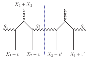
Refer to caption
Figure 7: Lowest order graph for the 2v1 mechanism, with the blobs connecting partons with hadrons being omitted at the top and the bottom. The vector boson with momentum q1subscript𝑞1q_{1} is understood to cross the final state cut. The four quark lines at the bottom are right moving, the two gluons entering at the top left moving.

Whereas the SPS contribution in the previous subsection gives a finite result when computed as a perturbative two-loop graph, the twist-four contribution has a collinear divergence when integrated over the full region of phase space. To exhibit this divergence, we use dimensional regularisation and write

dσtw4dx1dx2dx¯1dx¯2𝑑subscript𝜎tw4𝑑subscript𝑥1𝑑subscript𝑥2𝑑subscript¯𝑥1𝑑subscript¯𝑥2\displaystyle\frac{d\sigma_{\text{tw4}}}{dx_{1}\,dx_{2}\,d\bar{x}_{1}\,d\bar{x}_{2}} =dD2𝒒X1X2𝑑vX1X2𝑑va1a2Ga1a2(X1+v,X2v,X2v,X1+v)absentsuperscript𝑑𝐷2𝒒superscriptsubscriptsubscript𝑋1subscript𝑋2differential-d𝑣superscriptsubscriptsubscript𝑋1subscript𝑋2differential-dsuperscript𝑣subscriptsubscript𝑎1subscript𝑎2subscript𝐺subscript𝑎1subscript𝑎2subscript𝑋1𝑣subscript𝑋2𝑣subscript𝑋2superscript𝑣subscript𝑋1superscript𝑣\displaystyle=\int d^{D-2}\boldsymbol{q}\,\int_{-X_{1}}^{X_{2}}dv\int_{-X_{1}}^{X_{2}}dv^{\prime}\,\sum_{a_{1}a_{2}}G_{a_{1}a_{2}}(X_{1}+v,X_{2}-v,X_{2}-v^{\prime},X_{1}+v^{\prime})\,
×Ha1a2,g(𝒒,Xi,v,v,\macc@depthΔ\frozen@everymath\macc@group\macc@set@skewchar\macc@nested@a111Xi,s)fg(\macc@depthΔ\frozen@everymath\macc@group\macc@set@skewchar\macc@nested@a111X1+\macc@depthΔ\frozen@everymath\macc@group\macc@set@skewchar\macc@nested@a111X2)absentsubscript𝐻subscript𝑎1subscript𝑎2𝑔𝒒subscript𝑋𝑖𝑣superscript𝑣\macc@depthΔ\frozen@everymath\macc@group\macc@set@skewchar\macc@nested@a111subscript𝑋𝑖𝑠subscript𝑓𝑔\macc@depthΔ\frozen@everymath\macc@group\macc@set@skewchar\macc@nested@a111subscript𝑋1\macc@depthΔ\frozen@everymath\macc@group\macc@set@skewchar\macc@nested@a111subscript𝑋2\displaystyle\quad\times H_{a_{1}a_{2},g}(\boldsymbol{q},X_{i},v,v^{\prime},\macc@depth\char 1\relax\frozen@everymath{\macc@group}\macc@set@skewchar\macc@nested@a 111{X}_{i},s)\,f_{g}(\macc@depth\char 1\relax\frozen@everymath{\macc@group}\macc@set@skewchar\macc@nested@a 111{X}_{1}+\macc@depth\char 1\relax\frozen@everymath{\macc@group}\macc@set@skewchar\macc@nested@a 111{X}_{2})\,

As in the previous subsection, we restrict the meaning of σtw4subscript𝜎tw4\sigma_{\text{tw4}} and other terms in the cross section to the contribution from a single graph. The labels a1subscript𝑎1a_{1} and a2subscript𝑎2a_{2} indicate parton species and polarisation, and G𝐺G is a collinear twist-four distribution. H𝐻H includes overall factors and the squared amplitude of the hard scattering process qq¯+gV1V2𝑞¯𝑞𝑔subscript𝑉1subscript𝑉2q\bar{q}+g\to V_{1}V_{2}. Note that in the hard scattering graph one has 𝒒1=𝒒2=𝒒subscript𝒒1subscript𝒒2𝒒\boldsymbol{q}_{1}=-\boldsymbol{q}_{2}=\boldsymbol{q}. Momentum fractions are as shown in figure 7. The plus- and minus-momentum fractions of the produced bosons are respectively given by

Xisubscript𝑋𝑖\displaystyle X_{i} =qi+p+=Qi2+qi2Qi2xi,absentsuperscriptsubscript𝑞𝑖superscript𝑝superscriptsubscript𝑄𝑖2superscriptsubscript𝑞𝑖2superscriptsubscript𝑄𝑖2subscript𝑥𝑖\displaystyle=\frac{q_{i}^{+}}{p^{+}}=\sqrt{\frac{Q_{i}^{2}+{q}_{i}^{2}}{Q_{i}^{2}}}\,x_{i}\,, \macc@depthΔ\frozen@everymath\macc@group\macc@set@skewchar\macc@nested@a111Xi\macc@depthΔ\frozen@everymath\macc@group\macc@set@skewchar\macc@nested@a111subscript𝑋𝑖\displaystyle\macc@depth\char 1\relax\frozen@everymath{\macc@group}\macc@set@skewchar\macc@nested@a 111{X}_{i} =qip¯=Qi2+qi2Qi2x¯iabsentsuperscriptsubscript𝑞𝑖superscript¯𝑝superscriptsubscript𝑄𝑖2superscriptsubscript𝑞𝑖2superscriptsubscript𝑄𝑖2subscript¯𝑥𝑖\displaystyle=\frac{q_{i}^{-}}{\bar{p}^{\,-}}=\sqrt{\frac{Q_{i}^{2}+{q}_{i}^{2}}{Q_{i}^{2}}}\,\bar{x}_{i} (38)

with xisubscript𝑥𝑖x_{i} and x¯isubscript¯𝑥𝑖\bar{x}_{i} defined in (4). For the momenta of internal lines in the hard scattering subprocess, minus and transverse components are fixed by the final state kinematics, so that there is only a loop integration over the plus-momentum fractions v𝑣v and vsuperscript𝑣v^{\prime}. Note that by virtue of (38) both Xisubscript𝑋𝑖X_{i} and \macc@depthΔ\frozen@everymath\macc@group\macc@set@skewchar\macc@nested@a111Xi\macc@depthΔ\frozen@everymath\macc@group\macc@set@skewchar\macc@nested@a111subscript𝑋𝑖\macc@depth\char 1\relax\frozen@everymath{\macc@group}\macc@set@skewchar\macc@nested@a 111{X}_{i} have an implicit dependence on q2superscript𝑞2q^{2} at given xi,x¯isubscript𝑥𝑖subscript¯𝑥𝑖x_{i},\bar{x}_{i}. An upper limit on q2superscript𝑞2q^{2} follows from the requirements that X1+X21subscript𝑋1subscript𝑋21X_{1}+X_{2}\leq 1 and \macc@depthΔ\frozen@everymath\macc@group\macc@set@skewchar\macc@nested@a111X1+\macc@depthΔ\frozen@everymath\macc@group\macc@set@skewchar\macc@nested@a111X21\macc@depthΔ\frozen@everymath\macc@group\macc@set@skewchar\macc@nested@a111subscript𝑋1\macc@depthΔ\frozen@everymath\macc@group\macc@set@skewchar\macc@nested@a111subscript𝑋21\macc@depth\char 1\relax\frozen@everymath{\macc@group}\macc@set@skewchar\macc@nested@a 111{X}_{1}+\macc@depth\char 1\relax\frozen@everymath{\macc@group}\macc@set@skewchar\macc@nested@a 111{X}_{2}\leq 1.

The expression (4.1.2) includes a contribution from DPS region, characterised by qiQimuch-less-thansubscript𝑞𝑖subscript𝑄𝑖q_{i}\ll Q_{i} and v,v1much-less-than𝑣superscript𝑣1v,v^{\prime}\ll 1. Let us approximate the integrand in that region. We first perform a Fierz transformation for the Dirac indices of the upper quark lines at the gauge boson vertices and retain only the leading Dirac structures. After this, the cross sections σ^isubscript^𝜎𝑖\hat{\sigma}_{i} for qq¯𝑞¯𝑞q\bar{q} annihilation appear in the expression. Furthermore we set v=v=0𝑣superscript𝑣0v=v^{\prime}=0 in G𝐺G and extend the integrations over v𝑣v and vsuperscript𝑣v^{\prime} to the full real axis (after which they are easily done using Cauchy’s theorem). Approximating Xixisubscript𝑋𝑖subscript𝑥𝑖X_{i}\approx x_{i} and \macc@depthΔ\frozen@everymath\macc@group\macc@set@skewchar\macc@nested@a111Xix¯i\macc@depthΔ\frozen@everymath\macc@group\macc@set@skewchar\macc@nested@a111subscript𝑋𝑖subscript¯𝑥𝑖\macc@depth\char 1\relax\frozen@everymath{\macc@group}\macc@set@skewchar\macc@nested@a 111{X}_{i}\approx\bar{x}_{i} and collecting all factors, we obtain

dσtw4dx1dx2dx¯1dx¯2|qQi and v,v1=a1a2b1b2σ^a1b1σ^a2b2Ga1a2(x1,x2,x2,x1)evaluated-at𝑑subscript𝜎tw4𝑑subscript𝑥1𝑑subscript𝑥2𝑑subscript¯𝑥1𝑑subscript¯𝑥2formulae-sequencemuch-less-than𝑞subscript𝑄𝑖 and 𝑣much-less-thansuperscript𝑣1subscriptsubscript𝑎1subscript𝑎2subscript𝑏1subscript𝑏2subscript^𝜎subscript𝑎1subscript𝑏1subscript^𝜎subscript𝑎2subscript𝑏2subscript𝐺subscript𝑎1subscript𝑎2subscript𝑥1subscript𝑥2subscript𝑥2subscript𝑥1\displaystyle\frac{d\sigma_{\text{tw4}}}{dx_{1}\,dx_{2}\,d\bar{x}_{1}\,d\bar{x}_{2}}\bigg{|}_{q\ll Q_{i}\text{\leavevmode\nobreak\ and\leavevmode\nobreak\ }v,v^{\prime}\ll 1}=\sum_{a_{1}a_{2}b_{1}b_{2}}\hat{\sigma}_{a_{1}b_{1}}\mskip 1.5mu\hat{\sigma}_{a_{2}b_{2}}\mskip 1.5muG_{a_{1}a_{2}}(x_{1},x_{2},x_{2},x_{1})\,
×qQidD2𝒒𝒒j𝒒jq4(2μ)4DπD3αs2πTgb1b2jj(x¯1x¯1+x¯2)fg(x¯1+x¯2)x¯1+x¯2\displaystyle\qquad\quad\times\int\limits_{q\ll Q_{i}}d^{D-2}\boldsymbol{q}\;\frac{\boldsymbol{q}^{j}\boldsymbol{q}^{j^{\prime}}}{q^{4}}\,\frac{(2\mu)^{4-D}}{\pi^{D-3}}\,\frac{\alpha_{s}}{2\pi}\;T^{jj^{\prime}}_{g\to b_{1}b_{2}}\biggl{(}\frac{\bar{x}_{1}}{\bar{x}_{1}+\bar{x}_{2}}\biggr{)}\,\frac{f_{g}(\bar{x}_{1}+\bar{x}_{2})}{\bar{x}_{1}+\bar{x}_{2}} (39)

with the splitting kernel T𝑇T from (3.1). If we drop the restriction qQimuch-less-than𝑞subscript𝑄𝑖q\ll Q_{i}, then the expression in the second line of (4.1.2) becomes the perturbative splitting approximation Fspl,pt(x¯i,𝚫=𝟎)subscript𝐹spl,ptsubscript¯𝑥𝑖𝚫0F_{\text{spl,pt}}(\bar{x}_{i},\boldsymbol{\Delta}=\boldsymbol{0}) of the transverse-momentum integrated DPD. This DPD is evaluated at 𝚫=𝟎𝚫0\boldsymbol{\Delta}=\boldsymbol{0} in order to fulfil momentum conservation at the gauge boson vertices, because the transverse momenta of the right moving partons are set to zero in the overall hard scattering kernel H𝐻H.

The 𝒒𝒒\boldsymbol{q} integral of (4.1.2) has an infrared divergence in D=4𝐷4D=4 dimensions, which must be cancelled by the subtraction term for the DPS region. That term is obtained by applying the DPS approximations to the graph, in addition to those for the twist-four region. This gives again the form (4.1.2), but with an unrestricted integration over 𝒒𝒒\boldsymbol{q}, and a regulator of the corresponding ultraviolet divergence. To implement the regulator, we Fourier transform the collinear DPD, Fspl,pt(x¯i,𝚫=𝟎)=dD2𝒚Fspl,pt(x¯i,𝒚)subscript𝐹spl,ptsubscript¯𝑥𝑖𝚫0superscript𝑑𝐷2𝒚subscript𝐹spl,ptsubscript¯𝑥𝑖𝒚F_{\text{spl,pt}}(\bar{x}_{i},\boldsymbol{\Delta}=\boldsymbol{0})=\int d^{D-2}\boldsymbol{y}\;F_{\text{spl,pt}}(\bar{x}_{i},\boldsymbol{y}), and then multiply with Φ2(yν)superscriptΦ2𝑦𝜈\Phi^{2}(y\nu) as prescribed by our formalism. This gives

dσ2v1,ptdx1dx2dx¯1dx¯2𝑑subscript𝜎2v1,pt𝑑subscript𝑥1𝑑subscript𝑥2𝑑subscript¯𝑥1𝑑subscript¯𝑥2\displaystyle\frac{d\sigma_{\text{2v1,pt}}}{dx_{1}\,dx_{2}\,d\bar{x}_{1}\,d\bar{x}_{2}}
=a1a2b1b2σ^a1b1σ^a2b2Ga1a2(x1,x2,x2,x1)dD2𝒚Φ2(yν)Fb1b2spl,pt(x¯i,𝒚).absentsubscriptsubscript𝑎1subscript𝑎2subscript𝑏1subscript𝑏2subscript^𝜎subscript𝑎1subscript𝑏1subscript^𝜎subscript𝑎2subscript𝑏2subscript𝐺subscript𝑎1subscript𝑎2subscript𝑥1subscript𝑥2subscript𝑥2subscript𝑥1superscript𝑑𝐷2𝒚superscriptΦ2𝑦𝜈subscript𝐹subscript𝑏1subscript𝑏2spl,ptsubscript¯𝑥𝑖𝒚\displaystyle\quad=\sum_{a_{1}a_{2}b_{1}b_{2}}\hat{\sigma}_{a_{1}b_{1}}\mskip 1.5mu\hat{\sigma}_{a_{2}b_{2}}\mskip 1.5muG_{a_{1}a_{2}}(x_{1},x_{2},x_{2},x_{1})\,\int d^{D-2}\boldsymbol{y}\;\Phi^{2}(y\nu)\,F_{b_{1}b_{2}\,\text{spl,pt}}(\bar{x}_{i},\boldsymbol{y})\,. (40)

Alternatively, one can obtain the subtraction term by starting with the contribution σ2v1subscript𝜎2v1\sigma_{\text{2v1}} of graph 1b to the DPS cross section and applying the additional approximations adequate for the twist-four region. Let us translate the latter from transverse momentum (where the twist-four approximations are formulated) to transverse position (where our UV regulator for the DPS cross section is local). On the l.h.s. of the relation

dD2𝚫(2π)D2Fint(xi,𝚫)Fspl(x¯i,𝚫)superscript𝑑𝐷2𝚫superscript2𝜋𝐷2subscript𝐹intsubscript𝑥𝑖𝚫subscript𝐹splsubscript¯𝑥𝑖𝚫\displaystyle\int\frac{d^{D-2}\boldsymbol{\Delta}}{(2\pi)^{D-2}}\;F_{\text{int}}(x_{i},\boldsymbol{\Delta})\,F_{\text{spl}}(\bar{x}_{i},-\boldsymbol{\Delta}) =dD2𝒚Fint(xi,𝒚)Fspl(x¯i,𝒚)absentsuperscript𝑑𝐷2𝒚subscript𝐹intsubscript𝑥𝑖𝒚subscript𝐹splsubscript¯𝑥𝑖𝒚\displaystyle=\int d^{D-2}\boldsymbol{y}\;F_{\text{int}}(x_{i},\boldsymbol{y})\,F_{\text{spl}}(\bar{x}_{i},\boldsymbol{y}) (41)

one neglects 𝚫𝚫\boldsymbol{\Delta} in the upper part of the graph, replacing Fspl(x¯i,𝚫)subscript𝐹splsubscript¯𝑥𝑖𝚫F_{\text{spl}}(\bar{x}_{i},\boldsymbol{\Delta}) by its value at 𝚫=𝟎𝚫0\boldsymbol{\Delta}=\boldsymbol{0}. The integral over 𝚫𝚫\boldsymbol{\Delta} of Fint(xi,𝚫)subscript𝐹intsubscript𝑥𝑖𝚫F_{\text{int}}(x_{i},\boldsymbol{\Delta}) gives the collinear twist-four distribution G(x1,x2,x2,x1)𝐺subscript𝑥1subscript𝑥2subscript𝑥2subscript𝑥1G(x_{1},x_{2},x_{2},x_{1}). In 𝒚𝒚\boldsymbol{y} space this corresponds to replacing Fint(xi,𝒚)subscript𝐹intsubscript𝑥𝑖𝒚F_{\text{int}}(x_{i},\boldsymbol{y}) by its value at 𝒚=𝟎𝒚0\boldsymbol{y}=\boldsymbol{0} while retaining the 𝒚𝒚\boldsymbol{y} dependence of Fspl(x¯i,𝒚)subscript𝐹splsubscript¯𝑥𝑖𝒚F_{\text{spl}}(\bar{x}_{i},\boldsymbol{y}). Including the regulator function Φ2(yν)superscriptΦ2𝑦𝜈\Phi^{2}(y\nu) under the 𝒚𝒚\boldsymbol{y} integral, one gets Fint(xi,𝒚=𝟎)dD2𝒚Φ2(yν)Fspl(x¯i,𝒚)subscript𝐹intsubscript𝑥𝑖𝒚0superscript𝑑𝐷2𝒚superscriptΦ2𝑦𝜈subscript𝐹splsubscript¯𝑥𝑖𝒚F_{\text{int}}(x_{i},\boldsymbol{y}=\boldsymbol{0})\int d^{D-2}\boldsymbol{y}\;\Phi^{2}(y\nu)\,F_{\text{spl}}(\bar{x}_{i},\boldsymbol{y}). The twist-four approximation implies computing the gqq¯𝑔𝑞¯𝑞g\to q\bar{q} splitting in perturbation theory, with massless quarks and the gluons taken collinear and on shell. This corresponds to replacing Fsplsubscript𝐹splF_{\text{spl}} with Fspl,ptsubscript𝐹spl,ptF_{\text{spl,pt}}. For the graph under discussion one has Fint(xi,𝒚=𝟎)=G(x1,x2,x2,x1)subscript𝐹intsubscript𝑥𝑖𝒚0𝐺subscript𝑥1subscript𝑥2subscript𝑥2subscript𝑥1F_{\text{int}}(x_{i},\boldsymbol{y}=\boldsymbol{0})=G(x_{1},x_{2},x_{2},x_{1}) according to (30) and thus obtains (4.1.2). We see that, as in the case of the 1v1 graph, the subtraction term is obtained from the DPS cross section by replacing the DPDs with their small y𝑦y approximation at the appropriate order in αssubscript𝛼𝑠\alpha_{s}. In section 5 we will find that this also holds at higher orders, where we have to take into account the second term in (30).

Let us finally perform the 𝒚𝒚\boldsymbol{y} integral in the subtraction term (4.1.2). Collecting all 𝒚𝒚\boldsymbol{y} and ϵitalic-ϵ\epsilon dependent factors in (3.2), we have

I(μ,ν)𝐼𝜇𝜈\displaystyle I(\mu,\nu) =μ2ϵΓ2(1ϵ)π12ϵP(ϵ)d22ϵ𝒚y24ϵΦ2(yν)absentsuperscript𝜇2italic-ϵsuperscriptΓ21italic-ϵsuperscript𝜋12italic-ϵ𝑃italic-ϵsuperscript𝑑22italic-ϵ𝒚superscript𝑦24italic-ϵsuperscriptΦ2𝑦𝜈\displaystyle=\mu^{2\epsilon}\,\frac{\Gamma^{2}(1-\epsilon)}{\pi^{1-2\epsilon}}\,P(\epsilon)\int\frac{d^{2-2\epsilon}\boldsymbol{y}}{y^{2-4\epsilon}}\;\Phi^{2}(y\nu)
=(μν)2ϵΓ2(1ϵ)π12ϵP(ϵ)Ω22ϵ0duu12ϵΦ2(u),absentsuperscript𝜇𝜈2italic-ϵsuperscriptΓ21italic-ϵsuperscript𝜋12italic-ϵ𝑃italic-ϵsubscriptΩ22italic-ϵsuperscriptsubscript0𝑑𝑢superscript𝑢12italic-ϵsuperscriptΦ2𝑢\displaystyle=\biggl{(}\frac{\mu}{\nu}\biggr{)}^{2\epsilon}\,\frac{\Gamma^{2}(1-\epsilon)}{\pi^{1-2\epsilon}}\;P(\epsilon)\,\Omega_{2-2\epsilon}\int_{0}^{\infty}\frac{du}{u^{1-2\epsilon}}\;\Phi^{2}(u)\,, (42)

where Ω2n=2πn/Γ(n)subscriptΩ2𝑛2superscript𝜋𝑛Γ𝑛\Omega_{2n}=2\pi^{n}/\Gamma(n) is the surface of a sphere in 2n2𝑛2n dimensions. For brevity we do not display the momentum fraction in the splitting kernel P𝑃P. The 𝒚𝒚\boldsymbol{y} integral is infrared divergent in 222 dimensions and converges for ϵ<0italic-ϵ0\epsilon<0. Using the third row of table 1, we get in particular

I(μ,ν)𝐼𝜇𝜈\displaystyle I(\mu,\nu) =[1ϵlog(4π)+γ+logν2μ2]P(0)P(0)+𝒪(ϵ)absentdelimited-[]1italic-ϵ4𝜋𝛾superscript𝜈2superscript𝜇2𝑃0superscript𝑃0𝒪italic-ϵ\displaystyle=\biggl{[}-\frac{1}{\epsilon}-\log(4\pi)+\gamma+\log\frac{\nu^{2}}{\mu^{2}}\mskip 1.5mu\biggr{]}\,P(0)-P^{\prime}(0)+\mathcal{O}(\epsilon) (43)

for Φ(u)=Θ(ub0)Φ𝑢Θ𝑢subscript𝑏0\Phi(u)=\Theta(u-b_{0}), where P=P/ϵsuperscript𝑃𝑃italic-ϵP^{\prime}=\partial P/\partial\epsilon.

The contribution of the graph to the overall cross section is finally given by

σtw4σ2v1,pt+σ2v1,subscript𝜎tw4subscript𝜎2v1,ptsubscript𝜎2v1\displaystyle\sigma_{\text{tw4}}-\sigma_{\text{2v1,pt}}+\sigma_{\text{2v1}}\,, (44)

in analogy to (37). By the same argument as in the previous subsection, one finds that this combination reproduces the graph over the full range of y𝑦y values, with the second term cancelling against the third term for y1/Qsimilar-to𝑦1𝑄y\sim 1/Q and against the first term for y1/Qmuch-greater-than𝑦1𝑄y\gg 1/Q.

As we have just seen, the product of (μ/ν)2ϵsuperscript𝜇𝜈2italic-ϵ(\mu/\nu)^{2\epsilon} with the 1/ϵ1italic-ϵ1/\epsilon pole gives a logarithm log(ν/μ)𝜈𝜇\log(\nu/\mu) in the subtraction term σ2v1,ptsubscript𝜎2v1,pt\sigma_{\text{2v1,pt}}. In turn, the 𝒒𝒒\boldsymbol{q} integral in the expression (4.1.2) of σtw4subscript𝜎tw4\sigma_{\text{tw4}} gives log(Q/μ)𝑄𝜇\log(Q/\mu), where Q𝑄Q comes from the upper integration limit and the μ𝜇\mu dependence from the regulated infrared divergence. In the combination σtw4σ2v1,ptsubscript𝜎tw4subscript𝜎2v1,pt\sigma_{\text{tw4}}-\sigma_{\text{2v1,pt}} this gives log(Q/ν)𝑄𝜈\log(Q/\nu). The ν𝜈\nu dependence is cancelled by a log(ν/Λ)𝜈Λ\log(\nu/\Lambda) from the 𝒚𝒚\boldsymbol{y} integral of the DPS cross section σ2v1subscript𝜎2v1\sigma_{\text{2v1}}, where ν𝜈\nu regulates the ultraviolet divergence. Combining all terms, one obtains log(Q/Λ)𝑄Λ\log(Q/\Lambda) in (44). With the choice νQsimilar-to𝜈𝑄\nu\sim Q, the large part of the logarithm is contained only in the DPS term.

4.1.3 Combining contributions

We can now add all contributions to the physical cross section, including 1v1, 2v1 and 2v2 graphs in DPS. We include the same regulator Φ(yν)Φ𝑦𝜈\Phi(y\nu) in all DPD contributions, so that the splitting and intrinsic contributions to the individual DPDs can be added up to distributions F=Fspl+Fint𝐹subscript𝐹splsubscript𝐹intF=F_{\text{spl}}+F_{\text{int}} that are defined by operator matrix elements as described in section 2.

2v2 graphs like the one in figure 1c are dominated by the DPS region, where transverse parton momenta are small, whilst regions with large transverse momenta are subleading. In impact parameter space this means that including the ΦΦ\Phi regulator to suppress the region of small y𝑦y does not significantly change σ2v2subscript𝜎2v2\sigma_{\text{2v2}}. We will see in section 4.3 that the effect of ΦΦ\Phi in the 2v2 term is at the level of power corrections.

The master formula for the cross section with integrated transverse momenta is then

σ𝜎\displaystyle\sigma =σSPSσ1v1,pt+σtw4σ2v1,pt+σDPS,absentsubscript𝜎SPSsubscript𝜎1v1,ptsubscript𝜎tw4subscript𝜎2v1,ptsubscript𝜎DPS\displaystyle=\sigma_{\text{SPS}}-\sigma_{\text{1v1,pt}}+\sigma_{\text{tw4}}-\sigma_{\text{2v1,pt}}+\sigma_{\text{DPS}}\,, (45)

where σDPS=σ1v1+σ2v1+σ2v2subscript𝜎DPSsubscript𝜎1v1subscript𝜎2v1subscript𝜎2v2\sigma_{\text{DPS}}=\sigma_{\text{1v1}}+\sigma_{\text{2v1}}+\sigma_{\text{2v2}} includes all contributions to the DPS cross section and involves the full DPDs F𝐹F. From the discussion in the previous two subsections it follows that the ν𝜈\nu dependence of σDPSsubscript𝜎DPS\sigma_{\text{DPS}} cancels against the one of σ1v1,pt+σ2v1,ptsubscript𝜎1v1,ptsubscript𝜎2v1,pt\sigma_{\text{1v1,pt}}+\sigma_{\text{2v1,pt}}, up to terms of higher order in αssubscript𝛼𝑠\alpha_{s} that are beyond the accuracy of the calculation. As discussed in section 2.1 we neglect contributions involving twist-three functions in (45).

The terms in (45) are now meant to include all contributing graphs, including graphs without a double counting issue. The hard scattering cross sections needed for the DPS term are available for many final states, and σ1v1,ptsubscript𝜎1v1,pt\sigma_{\text{1v1,pt}} can be readily obtained from existing results at leading order in αssubscript𝛼𝑠\alpha_{s}. For double gauge boson production, the SPS cross section has been computed at high perturbative order, including the double box graphs as well as the first radiative corrections to them Caola:2016trd . On the other hand, to the best of our knowledge, no calculations of σtw4subscript𝜎tw4\sigma_{\text{tw4}} have been performed so far. To leading logarithmic accuracy, one can however omit the terms σtw4σ2v1,ptsubscript𝜎tw4subscript𝜎2v1,pt\sigma_{\text{tw4}}-\sigma_{\text{2v1,pt}} in (45), because with the choice νQsimilar-to𝜈𝑄\nu\sim Q the large DPS logarithm log(Q/Λ)𝑄Λ\log(Q/\Lambda) generated by 2v1 graphs is entirely contained in σDPSsubscript𝜎DPS\sigma_{\text{DPS}}, as discussed in the previous subsection.

4.2 Leading order analysis: TMD factorisation

We now show how our formalism works for TMD factorisation. As explained in section 2.1, the cross section for q1,q2Qmuch-less-thansubscript𝑞1subscript𝑞2𝑄q_{1},q_{2}\ll Q receives leading-power contributions from DPS, SPS and from their interference. The 2v1 contribution is power suppressed in this case and will not be discussed further in this subsection. The discussion of leading momentum regions is a bit more involved now, because the two quark loops in the double box graph can be collinear or hard independently of each other.

We start with the SPS/DPS interference, for which a graph is shown in figure 2b. Its contribution to the V1V2subscript𝑉1subscript𝑉2V_{1}V_{2} production cross section has the form

dσDPS/SPSdx1dx2dx¯1dx¯2d2𝒒1d2𝒒2𝑑subscript𝜎DPS/SPS𝑑subscript𝑥1𝑑subscript𝑥2𝑑subscript¯𝑥1𝑑subscript¯𝑥2superscript𝑑2subscript𝒒1superscript𝑑2subscript𝒒2\displaystyle\frac{d\sigma_{\text{DPS/SPS}}}{dx_{1}\,dx_{2}\,d\bar{x}_{1}\,d\bar{x}_{2}\,d^{2}\boldsymbol{q}_{1}\,d^{2}\boldsymbol{q}_{2}} α1,α2,α0β1,β2,β0Hα1β1Hα2β2Hα0β0d2𝒁d2𝒚+ei(𝒒1+𝒒2)𝒁i𝒒𝒚+proportional-toabsentsubscriptFRACOPsubscript𝛼1subscript𝛼2subscript𝛼0subscript𝛽1subscript𝛽2subscript𝛽0subscript𝐻subscript𝛼1subscript𝛽1subscript𝐻subscript𝛼2subscript𝛽2subscriptsuperscript𝐻subscript𝛼0subscript𝛽0superscript𝑑2𝒁superscript𝑑2subscript𝒚superscript𝑒𝑖subscript𝒒1subscript𝒒2𝒁𝑖𝒒subscript𝒚\displaystyle\,\propto\,\sum_{\genfrac{}{}{0.0pt}{1}{\alpha_{1},\alpha_{2},\alpha_{0}}{\beta_{1},\beta_{2},\beta_{0}}}H_{\alpha_{1}\beta_{1}}\,H_{\alpha_{2}\beta_{2}}\,H^{*}_{\alpha_{0}\beta_{0}}\int d^{2}\boldsymbol{Z}\,d^{2}\boldsymbol{y}_{+}\;e^{-i(\boldsymbol{q}_{1}+\boldsymbol{q}_{2})\boldsymbol{Z}-i\boldsymbol{q}\boldsymbol{y}_{+}}
×Φ(y+ν)Dβ1β2|β0(x¯i,𝒚+,𝒁)Dα1α2|α0(xi,𝒚+,𝒁),absentΦsubscript𝑦𝜈subscript𝐷conditionalsubscript𝛽1subscript𝛽2subscript𝛽0subscript¯𝑥𝑖subscript𝒚𝒁subscript𝐷conditionalsubscript𝛼1subscript𝛼2subscript𝛼0subscript𝑥𝑖subscript𝒚𝒁\displaystyle\qquad\times\Phi(y_{+}\nu)\,D_{\beta_{1}\beta_{2}|\beta_{0}}(\bar{x}_{i},\boldsymbol{y}_{+},\boldsymbol{Z})\,D_{\alpha_{1}\alpha_{2}|\alpha_{0}}(x_{i},\boldsymbol{y}_{+},\boldsymbol{Z})\,,
dσSPS/DPSdx1dx2dx¯1dx¯2d2𝒒1d2𝒒2𝑑subscript𝜎SPS/DPS𝑑subscript𝑥1𝑑subscript𝑥2𝑑subscript¯𝑥1𝑑subscript¯𝑥2superscript𝑑2subscript𝒒1superscript𝑑2subscript𝒒2\displaystyle\frac{d\sigma_{\text{SPS/DPS}}}{dx_{1}\,dx_{2}\,d\bar{x}_{1}\,d\bar{x}_{2}\,d^{2}\boldsymbol{q}_{1}\,d^{2}\boldsymbol{q}_{2}} α0,α1,α2β0,β1,β2Hα0β0Hα1β1Hα2β2d2𝒁d2𝒚ei(𝒒1+𝒒2)𝒁+i𝒒𝒚proportional-toabsentsubscriptFRACOPsubscript𝛼0subscript𝛼1subscript𝛼2subscript𝛽0subscript𝛽1subscript𝛽2subscript𝐻subscript𝛼0subscript𝛽0subscriptsuperscript𝐻subscript𝛼1subscript𝛽1subscriptsuperscript𝐻subscript𝛼2subscript𝛽2superscript𝑑2𝒁superscript𝑑2subscript𝒚superscript𝑒𝑖subscript𝒒1subscript𝒒2𝒁𝑖𝒒subscript𝒚\displaystyle\,\propto\,\sum_{\genfrac{}{}{0.0pt}{1}{\alpha_{0},\alpha_{1},\alpha_{2}}{\beta_{0},\beta_{1},\beta_{2}}}H_{\alpha_{0}\beta_{0}}\,H^{*}_{\alpha_{1}\beta_{1}}\,H^{*}_{\alpha_{2}\beta_{2}}\int d^{2}\boldsymbol{Z}\,d^{2}\boldsymbol{y}_{-}\;e^{-i(\boldsymbol{q}_{1}+\boldsymbol{q}_{2})\boldsymbol{Z}+i\boldsymbol{q}\boldsymbol{y}_{-}}
×Φ(yν)Dβ0|β1β2(x¯i,𝒚,𝒁)Dα0|α1α2(xi,𝒚,𝒁)absentΦsubscript𝑦𝜈subscript𝐷conditionalsubscript𝛽0subscript𝛽1subscript𝛽2subscript¯𝑥𝑖subscript𝒚𝒁subscript𝐷conditionalsubscript𝛼0subscript𝛼1subscript𝛼2subscript𝑥𝑖subscript𝒚𝒁\displaystyle\qquad\times\Phi(y_{-}\nu)\,D_{\beta_{0}|\beta_{1}\beta_{2}}(\bar{x}_{i},\boldsymbol{y}_{-},\boldsymbol{Z})\,D_{\alpha_{0}|\alpha_{1}\alpha_{2}}(x_{i},\boldsymbol{y}_{-},\boldsymbol{Z}) (46)

for DPS in the amplitude or in its complex conjugate. Here D𝐷D are the twist-three TMDs introduced in section 3.1 and the proportionality is up to kinematic and numerical factors. We have different hard scattering amplitudes H𝐻H, with α0subscript𝛼0\alpha_{0} and β0subscript𝛽0\beta_{0} being gluons and the remaining partons quarks or antiquarks . The regions of small y+subscript𝑦y_{+} or ysubscript𝑦y_{-} are regulated by Φ(y+ν)Φsubscript𝑦𝜈\Phi(y_{+}\nu) and Φ(yν)Φsubscript𝑦𝜈\Phi(y_{-}\nu).

Notice that the graph in figure 2b has a leading contribution when the gqq¯𝑔𝑞¯𝑞g\to q\bar{q} splittings in the conjugate amplitude become collinear, in which case we are back in the DPS region. From the first expression in (4.2) one should therefore subtract

dσDPS,y0dx1dx2dx¯1dx¯2d2𝒒1d2𝒒2α1,α2β1,β2Hα1β1Hα2β2Hα1β1Hα2β2proportional-to𝑑subscript𝜎DPSsubscript𝑦0𝑑subscript𝑥1𝑑subscript𝑥2𝑑subscript¯𝑥1𝑑subscript¯𝑥2superscript𝑑2subscript𝒒1superscript𝑑2subscript𝒒2subscriptFRACOPsubscript𝛼1subscript𝛼2subscript𝛽1subscript𝛽2subscript𝐻subscript𝛼1subscript𝛽1subscript𝐻subscript𝛼2subscript𝛽2subscriptsuperscript𝐻subscript𝛼1subscript𝛽1subscriptsuperscript𝐻subscript𝛼2subscript𝛽2\displaystyle\frac{d\sigma_{\text{DPS},\,y_{-}\to 0}}{dx_{1}\,dx_{2}\,d\bar{x}_{1}\,d\bar{x}_{2}\,d^{2}\boldsymbol{q}_{1}\,d^{2}\boldsymbol{q}_{2}}\,\propto\,\sum_{\genfrac{}{}{0.0pt}{1}{\alpha_{1},\alpha_{2}}{\beta_{1},\beta_{2}}}H_{\alpha_{1}\beta_{1}}\,H_{\alpha_{2}\beta_{2}}\,H^{*}_{\alpha_{1}\beta_{1}}\,H^{*}_{\alpha_{2}\beta_{2}}\,
×d2𝒁d2𝒚+d2𝒚ei(𝒒1+𝒒2)𝒁i𝒒(𝒚+𝒚)Φ(y+ν)Φ(yν)\displaystyle\qquad\qquad\times\int d^{2}\boldsymbol{Z}\,d^{2}\boldsymbol{y}_{+}\,d^{2}\boldsymbol{y}_{-}\;e^{-i(\boldsymbol{q}_{1}+\boldsymbol{q}_{2})\boldsymbol{Z}-i\boldsymbol{q}(\boldsymbol{y}_{+}-\boldsymbol{y}_{-})}\,\Phi(y_{+}\nu)\,\Phi(y_{-}\nu)\,
×Fβ1β2,y0(x¯i,𝒚±,𝒁)Fα1α2,y0(xi,𝒚±,𝒁)absentsubscript𝐹subscript𝛽1subscript𝛽2subscript𝑦0subscript¯𝑥𝑖subscript𝒚plus-or-minus𝒁subscript𝐹subscript𝛼1subscript𝛼2subscript𝑦0subscript𝑥𝑖subscript𝒚plus-or-minus𝒁\displaystyle\qquad\qquad\quad\times F_{\beta_{1}\beta_{2},\mskip 1.5muy_{-}\to 0}(\bar{x}_{i},\boldsymbol{y}_{\pm},\boldsymbol{Z})\,F_{\alpha_{1}\alpha_{2},\mskip 1.5muy_{-}\to 0}(x_{i},\boldsymbol{y}_{\pm},\boldsymbol{Z}) (47)

with Fy0subscript𝐹subscript𝑦0F_{y_{-}\to 0} given in (19) and represented in figure 5b. From the second expression in (4.2) one should subtract an analogous term with y+0subscript𝑦0y_{+}\to 0.

According to (18), the computation of the subtraction terms involves the integrals

0dyyJn(yq)Φ(yν)superscriptsubscript0𝑑𝑦𝑦subscript𝐽𝑛𝑦𝑞Φ𝑦𝜈\displaystyle\int_{0}^{\infty}\frac{dy}{y}\,J_{n}(yq)\,\Phi(y\nu) =0duuJn(uq/ν)Φ(u)absentsuperscriptsubscript0𝑑𝑢𝑢subscript𝐽𝑛𝑢𝑞𝜈Φ𝑢\displaystyle=\int_{0}^{\infty}\frac{du}{u}\,J_{n}(uq/\nu)\,\Phi(u) with n=0,2,with 𝑛02\displaystyle\text{with\leavevmode\nobreak\ \leavevmode\nobreak\ }n=0,2, (48)

which are given in the appendix. We see in table 1 that for n=0𝑛0n=0 both our choices for ΦΦ\Phi give a logarithmic behaviour log(ν/q)𝜈𝑞\log(\nu/q) when νqmuch-greater-than𝜈𝑞\nu\gg q, as expected for a regulated logarithmically divergent integral.

Let us now turn to the double box graph. It has leading contributions when the loops are both hard (SPS region) or both collinear (DPS region), or when one loop is hard and the other one collinear (region of SPS/DPS interference). The terms to be added to the SPS cross section for removing the contribution from the SPS/DPS interference regions are

[dσDPS/SPS,y+0dx1dx2dx¯1dx¯2d2𝒒1d2𝒒2dσDPS,y±0dx1dx2dx¯1dx¯2d2𝒒1d2𝒒2]delimited-[]𝑑subscript𝜎DPS/SPSsubscript𝑦0𝑑subscript𝑥1𝑑subscript𝑥2𝑑subscript¯𝑥1𝑑subscript¯𝑥2superscript𝑑2subscript𝒒1superscript𝑑2subscript𝒒2𝑑subscript𝜎DPSsubscript𝑦plus-or-minus0𝑑subscript𝑥1𝑑subscript𝑥2𝑑subscript¯𝑥1𝑑subscript¯𝑥2superscript𝑑2subscript𝒒1superscript𝑑2subscript𝒒2\displaystyle-\biggl{[}\frac{d\sigma_{\text{DPS/SPS},\,y_{+}\to\mskip 1.5mu0}}{dx_{1}\mskip 1.5mudx_{2}\,d\bar{x}_{1}\mskip 1.5mud\bar{x}_{2}\,d^{2}\boldsymbol{q}_{1}\,d^{2}\boldsymbol{q}_{2}}-\frac{d\sigma_{\text{DPS},\,y_{\pm}\to\mskip 1.5mu0}}{dx_{1}\,dx_{2}\,d\bar{x}_{1}\,d\bar{x}_{2}\,d^{2}\boldsymbol{q}_{1}\,d^{2}\boldsymbol{q}_{2}}\biggr{]}
[dσSPS/DPS,y0dx1dx2dx¯1dx¯2d2𝒒1d2𝒒2dσDPS,y±0dx1dx2dx¯1dx¯2d2𝒒1d2𝒒2].delimited-[]𝑑subscript𝜎SPS/DPSsubscript𝑦0𝑑subscript𝑥1𝑑subscript𝑥2𝑑subscript¯𝑥1𝑑subscript¯𝑥2superscript𝑑2subscript𝒒1superscript𝑑2subscript𝒒2𝑑subscript𝜎DPSsubscript𝑦plus-or-minus0𝑑subscript𝑥1𝑑subscript𝑥2𝑑subscript¯𝑥1𝑑subscript¯𝑥2superscript𝑑2subscript𝒒1superscript𝑑2subscript𝒒2\displaystyle-\biggl{[}\frac{d\sigma_{\text{SPS/DPS},\,y_{-}\to\mskip 1.5mu0}}{dx_{1}\mskip 1.5mudx_{2}\,d\bar{x}_{1}\mskip 1.5mud\bar{x}_{2}\,d^{2}\boldsymbol{q}_{1}\,d^{2}\boldsymbol{q}_{2}}-\frac{d\sigma_{\text{DPS},\,y_{\pm}\to\mskip 1.5mu0}}{dx_{1}\,dx_{2}\,d\bar{x}_{1}\,d\bar{x}_{2}\,d^{2}\boldsymbol{q}_{1}\,d^{2}\boldsymbol{q}_{2}}\biggr{]}\,. (49)

The first terms in the square brackets are obtained from (4.2) by taking the perturbative splitting form for all distributions, the one for Dα1α2|α0(xi,𝒚+,𝒁)subscript𝐷conditionalsubscript𝛼1subscript𝛼2subscript𝛼0subscript𝑥𝑖subscript𝒚𝒁D_{\alpha_{1}\alpha_{2}|\alpha_{0}}(x_{i},\boldsymbol{y}_{+},\boldsymbol{Z}) being given in (21). The second terms are obtained from (4.2) and its analogue for y+0subscript𝑦0y_{+}\to 0 by taking both splitting vertices perturbative, using the DPD given in (3.1). Notice that the subtraction terms (4.2) contain subtractions themselves, showing the recursive nature of the construction in (31). Finally, one should remove the contribution from the DPS region by adding

dσDPS,y±0dx1dx2dx¯1dx¯2d2𝒒1d2𝒒2,𝑑subscript𝜎DPSsubscript𝑦plus-or-minus0𝑑subscript𝑥1𝑑subscript𝑥2𝑑subscript¯𝑥1𝑑subscript¯𝑥2superscript𝑑2subscript𝒒1superscript𝑑2subscript𝒒2\displaystyle{}-\frac{d\sigma_{\text{DPS},\,y_{\pm}\to\mskip 1.5mu0}}{dx_{1}\,dx_{2}\,d\bar{x}_{1}\,d\bar{x}_{2}\,d^{2}\boldsymbol{q}_{1}\,d^{2}\boldsymbol{q}_{2}}\,, (50)

where again both splitting vertices in each DPD are taken as perturbative. Note that in both (4.2) and (50) all proton matrix elements are expressed in terms of ordinary twist-two TMDs, as is the case for the SPS cross section.

Adding up contributions and double counting subtractions, we finally obtain

σ=σDPS𝜎subscript𝜎DPS\displaystyle\sigma=\sigma_{\text{DPS}\rule{0.0pt}{3.91806pt}} +[σDPS/SPSσDPS,y0+σSPS/DPSσDPS,y+0]delimited-[]subscript𝜎DPS/SPSsubscript𝜎DPSsubscript𝑦0subscript𝜎SPS/DPSsubscript𝜎DPSsubscript𝑦0\displaystyle+\bigl{[}\mskip 1.5mu\sigma_{\text{DPS/SPS}}-\sigma_{\text{DPS},\,y_{-}\to 0\rule{0.0pt}{3.91806pt}}+\sigma_{\text{SPS/DPS}}-\sigma_{\text{DPS},\,y_{+}\to 0\rule{0.0pt}{3.91806pt}}\mskip 1.5mu\bigr{]}
+[σSPSσDPS/SPS,y+0σSPS/DPS,y0+σDPS,y±0],delimited-[]subscript𝜎SPSsubscript𝜎DPS/SPSsubscript𝑦0subscript𝜎SPS/DPSsubscript𝑦0subscript𝜎DPSsubscript𝑦plus-or-minus0\displaystyle+\bigl{[}\mskip 1.5mu\sigma_{\text{SPS}\rule{0.0pt}{3.91806pt}}-\sigma_{\text{DPS/SPS},\,y_{+}\to 0}-\sigma_{\text{SPS/DPS},\,y_{-}\to 0}+\sigma_{\text{DPS},\,y_{\pm}\to 0}\rule{0.0pt}{5.59721pt}\mskip 1.5mu\bigr{]}\,, (51)

where we have again omitted differentials dx1dx2𝑑subscript𝑥1𝑑subscript𝑥2dx_{1}\,dx_{2}\,\ldots for brevity. The DPS cross section σDPSsubscript𝜎DPS\sigma_{\text{DPS}} contains contributions with and without splitting in each of the DPDs, which are defined by operator matrix elements as in the case of collinear factorisation.

Let us now discuss the large logarithms appearing in the different terms. The hard scattering kernel Hα0β0subscript𝐻subscript𝛼0subscript𝛽0H_{\alpha_{0}\beta_{0}} in (4.2) has a DPS logarithm log(Q/q)𝑄𝑞\log(Q/q), and correspondingly there is a log2(Q/q)superscript2𝑄𝑞\log^{2}(Q/q) in the unsubtracted SPS cross section. We take νQsimilar-to𝜈𝑄\nu\sim Q, so that these logarithms are fully removed by the double counting subtractions. They reappear in the logarithmic integrals over 𝒚+subscript𝒚\boldsymbol{y}_{+} and 𝒚subscript𝒚\boldsymbol{y}_{-} in the DPS cross section and in the SPS/DPS interference terms (4.2). In the full cross section (4.2) one then has a squared logarithm log2(Q/q)superscript2𝑄𝑞\log^{2}(Q/q) in the DPS term, and a single log(Q/q)𝑄𝑞\log(Q/q) in the subtracted SPS/DPS interference in the first line, whereas the subtracted SPS contribution in the last line has no leading logarithm. If q𝑞q is in the nonperturbative region, one has log(Q/Λ)𝑄Λ\log(Q/\Lambda) instead of log(Q/q)𝑄𝑞\log(Q/q).

At a practical level, the computation of the SPS/DPS interference requires twist-three TMDs as input, and the DPS term requires transverse-momentum dependent DPDs. In general, the modelling of these functions is very difficult and largely unconstrained. The situation is much better when q1,q2Λmuch-greater-thansubscript𝑞1subscript𝑞2Λq_{1},q_{2}\gg\Lambda: in this case one can compute these functions in terms of collinear ones Buffing:2016wip .

On the perturbative side, the calculation of the hard scattering cross sections in the DPS term is easiest, while the SPS and interference terms require the full computation of box graphs. If one is satisfied with keeping only the leading double logarithm in Q/q𝑄𝑞Q/q, then it is sufficient to retain only the DPS contribution with νQsimilar-to𝜈𝑄\nu\sim Q.

4.3 Subtraction formalism in momentum space

In Collins:2011zzd it was proven that the subtraction formalism leading to (31) correctly approximates a graph up to power suppressed terms, provided that each approximant TRsubscript𝑇𝑅T_{R} correctly reproduces the graph in its design region R𝑅R, up to power suppressed terms. This proof works with regions in momentum space. However, our UV regulator ΦΦ\Phi for DPS singularities is multiplicative in 𝒚𝒚\boldsymbol{y} space, which gives convolutions in transverse momenta that do not appear in the original Feynman graphs and hence are not part of the proof in Collins:2011zzd . We now show that this does not cause problems, so that our setup gives adequate approximations when transformed to momentum space, with corrections that are subleading in powers of Λ/νΛ𝜈\Lambda/\nu. With νQsimilar-to𝜈𝑄\nu\sim Q these corrections are of the same order as other approximations in the factorisation formula.

We begin with the case of collinear factorisation, using dimensional regularisation for UV and IR divergences as usual. As mentioned earlier, we choose ΦΦ\Phi such that the Fourier transform

Ψ(𝚫,ν)Ψ𝚫𝜈\displaystyle\Psi(\boldsymbol{\Delta},\nu) =dD2𝒚(2π)D2ei𝒚𝚫[1Φ2(yν)]=1νD2dD2𝒖(2π)D2ei𝒖𝚫/ν[1Φ2(u)].absentsuperscript𝑑𝐷2𝒚superscript2𝜋𝐷2superscript𝑒𝑖𝒚𝚫delimited-[]1superscriptΦ2𝑦𝜈1superscript𝜈𝐷2superscript𝑑𝐷2𝒖superscript2𝜋𝐷2superscript𝑒𝑖𝒖𝚫𝜈delimited-[]1superscriptΦ2𝑢\displaystyle=\int\frac{d^{D-2}\boldsymbol{y}}{(2\pi)^{D-2}}\;e^{-i\boldsymbol{y}\boldsymbol{\Delta}}\bigl{[}1-\Phi^{2}(y\nu)\bigr{]}=\frac{1}{\nu^{D-2}}\int\frac{d^{D-2}\boldsymbol{u}}{(2\pi)^{D-2}}\;e^{-i\boldsymbol{u}\boldsymbol{\Delta}/\nu}\bigl{[}1-\Phi^{2}(u)\bigr{]}\,. (52)

is finite for all values of Δ/νΔ𝜈\Delta/\nu. In the following we show that terms that depend on ΨΨ\Psi in the cross section are power suppressed and can hence be discarded when establishing the validity of the subtraction formalism.

Let us first discuss σ2v2subscript𝜎2v2\sigma_{\text{2v2}}, which is proportional to

(2π)D2superscript2𝜋𝐷2\displaystyle(2\pi)^{D-2}\!\int dD2𝒚Φ2(yν)Fint(𝒚)Fint(𝒚)=dD2𝚫Fint(𝚫)Fint(𝚫)superscript𝑑𝐷2𝒚superscriptΦ2𝑦𝜈subscript𝐹int𝒚subscript𝐹int𝒚superscript𝑑𝐷2𝚫subscript𝐹int𝚫subscript𝐹int𝚫\displaystyle d^{D-2}\boldsymbol{y}\;\Phi^{2}(y\nu)\mskip 1.5muF_{\text{int}}(\boldsymbol{y})\mskip 1.5muF_{\text{int}}(\boldsymbol{y})=\int d^{D-2}\boldsymbol{\Delta}\,F_{\text{int}}(\boldsymbol{\Delta})F_{\text{int}}(-\boldsymbol{\Delta})
dD2𝚫dD2𝚫Ψ(𝚫𝚫)Fint(𝚫)Fint(𝚫).superscript𝑑𝐷2𝚫superscript𝑑𝐷2superscript𝚫Ψ𝚫superscript𝚫subscript𝐹int𝚫subscript𝐹intsuperscript𝚫\displaystyle\quad-\int d^{D-2}\boldsymbol{\Delta}\,d^{D-2}\boldsymbol{\Delta}^{\prime}\;\Psi(\boldsymbol{\Delta}-\boldsymbol{\Delta}^{\prime})\,F_{\text{int}}(\boldsymbol{\Delta})\mskip 1.5muF_{\text{int}}(-\boldsymbol{\Delta}^{\prime})\,. (53)

The product σ^1σ^2subscript^𝜎1subscript^𝜎2\hat{\sigma}_{1}\mskip 1.5mu\hat{\sigma}_{2} of hard scattering cross sections does not affect our argument and is hence omitted. To keep the notation simple, we only display transverse-momentum arguments in this subsection. For simplicity we perform the power counting for D=4𝐷4D=4 dimensions; changes in D=42ϵ𝐷42italic-ϵD=4-2\epsilon are by fractional powers and do not alter our conclusions. We then have

Ψ(𝚫)Ψ𝚫\displaystyle\Psi(\boldsymbol{\Delta}) 1/ν2,similar-toabsent1superscript𝜈2\displaystyle\sim 1/\nu^{2}\,, Fint(𝚫)subscript𝐹int𝚫\displaystyle F_{\text{int}}(\boldsymbol{\Delta}) Λ2/Δ2similar-toabsentsuperscriptΛ2superscriptΔ2\displaystyle\sim\Lambda^{2}/\Delta^{2} (54)

for both ΔΛsimilar-toΔΛ\Delta\sim\Lambda and Δνsimilar-toΔ𝜈\Delta\sim\nu, which are the two scales present in (4.3).555In the ultraviolet region Δνmuch-greater-thanΔ𝜈\Delta\gg\nu there is a further suppression of Ψ(𝚫)Ψ𝚫\Psi(\boldsymbol{\Delta}) compared with 1/ν21superscript𝜈21/\nu^{2}, the exact form of which depends on the function ΦΦ\Phi. The large ΔΔ\Delta behaviour of Fintsubscript𝐹intF_{\text{int}} follows from dimensional analysis (Λ2superscriptΛ2\Lambda^{2} in the numerator comes from a collinear twist-four matrix element and 1/Δ21superscriptΔ21/\Delta^{2} from the hard splitting kernel in the Fourier transformed version of (30)). The ΨΨ\Psi independent term in (4.3) receives its leading contribution of order Λ2superscriptΛ2\Lambda^{2} from the region ΔΛsimilar-toΔΛ\Delta\sim\Lambda, which is the design region of the DPS approximation. By contrast, the ΨΨ\Psi dependent term behaves like Λ4/ν2superscriptΛ4superscript𝜈2\Lambda^{4}/\nu^{2}, with contributions from both ΔΛsimilar-toΔΛ\Delta\sim\Lambda and Δνsimilar-toΔ𝜈\Delta\sim\nu. We thus see that our UV regulator (which is not necessary in σ2v2subscript𝜎2v2\sigma_{\text{2v2}} as noted earlier) only gives changes suppressed by Λ2/ν2superscriptΛ2superscript𝜈2\Lambda^{2}/\nu^{2}. For νQsimilar-to𝜈𝑄\nu\sim Q this does not degrade the overall accuracy of the calculation.

Next we consider the contribution σ2v1σ2v1,pt+σtw4subscript𝜎2v1subscript𝜎2v1,ptsubscript𝜎tw4\sigma_{\text{2v1}}-\sigma_{\text{2v1,pt}}+\sigma_{\text{tw4}} from 2v1 graphs. Here we have a subtraction term, which is obtained by replacing the DPDs in 𝒚𝒚\boldsymbol{y} space with their perturbative approximations. In momentum space this reads

Fspl(𝚫)subscript𝐹spl𝚫\displaystyle F_{\text{spl}}(\boldsymbol{\Delta}) Fspl,pt(𝚫)absentsubscript𝐹spl,pt𝚫\displaystyle\to F_{\text{spl,pt}}(\boldsymbol{\Delta})
Fint(𝚫)subscript𝐹int𝚫\displaystyle F_{\text{int}}(\boldsymbol{\Delta}) Fint,pt(𝚫)+δ(D2)(𝚫)dD2𝚫[Fint(𝚫)Fint,pt(𝚫)].absentsubscript𝐹int,pt𝚫superscript𝛿𝐷2𝚫superscript𝑑𝐷2superscript𝚫delimited-[]subscript𝐹intsuperscript𝚫subscript𝐹int,ptsuperscript𝚫\displaystyle\to F_{\text{int,pt}}(\boldsymbol{\Delta})+\delta^{(D-2)}(\boldsymbol{\Delta})\,\int d^{D-2}\boldsymbol{\Delta}^{\prime}\,\bigl{[}F_{\text{int}}(\boldsymbol{\Delta}^{\prime})-F_{\text{int,pt}}(\boldsymbol{\Delta}^{\prime})\bigr{]}\,. (55)

The second line is obtained by replacing F𝐹F with Fintsubscript𝐹intF_{\text{int}} in the first term and with Fint,ptsubscript𝐹int,ptF_{\text{int,pt}} in the second term on the r.h.s. of (28) and then taking the Fourier transform with respect to 𝒚𝒚\boldsymbol{y}. We thus find that σ2v1σ2v1,ptsubscript𝜎2v1subscript𝜎2v1,pt\sigma_{\text{2v1}}-\sigma_{\text{2v1,pt}} is proportional to

(2π)D2dD2𝒚Φ2(yν)[Fspl(𝒚)Fint(𝒚)Fspl,pt(𝒚)Fint,pt(𝒚)]superscript2𝜋𝐷2superscript𝑑𝐷2𝒚superscriptΦ2𝑦𝜈delimited-[]subscript𝐹spl𝒚subscript𝐹int𝒚subscript𝐹spl,pt𝒚subscript𝐹int,pt𝒚\displaystyle(2\pi)^{D-2}\!\int d^{D-2}\boldsymbol{y}\;\Phi^{2}(y\nu)\mskip 1.5mu\bigl{[}F_{\text{spl}}(\boldsymbol{y})\mskip 1.5muF_{\text{int}}(\boldsymbol{y})-F_{\text{spl,pt}}(\boldsymbol{y})\mskip 1.5muF_{\text{int,pt}}(\boldsymbol{y})\bigr{]}
=dD2𝚫[Fspl(𝚫)Fint(𝚫)Fspl,pt(𝚫)Fint,pt(𝚫)]absentsuperscript𝑑𝐷2𝚫delimited-[]subscript𝐹spl𝚫subscript𝐹int𝚫subscript𝐹spl,pt𝚫subscript𝐹int,pt𝚫\displaystyle\quad=\int d^{D-2}\boldsymbol{\Delta}\,\bigl{[}F_{\text{spl}}(\boldsymbol{\Delta})\mskip 1.5muF_{\text{int}}(-\boldsymbol{\Delta})-F_{\text{spl,pt}}(\boldsymbol{\Delta})F_{\text{int,pt}}(-\boldsymbol{\Delta})\bigr{]}
Fspl,pt(𝚫=𝟎)dD2𝚫[Fint(𝚫)Fint,pt(𝚫)]subscript𝐹spl,pt𝚫0superscript𝑑𝐷2superscript𝚫delimited-[]subscript𝐹intsuperscript𝚫subscript𝐹int,ptsuperscript𝚫\displaystyle\qquad-F_{\text{spl,pt}}(\boldsymbol{\Delta}\!=\!\boldsymbol{0})\int d^{D-2}\boldsymbol{\Delta}^{\prime}\;\bigl{[}F_{\text{int}}(\boldsymbol{\Delta}^{\prime})-F_{\text{int,pt}}(\boldsymbol{\Delta}^{\prime})\bigr{]}
dD2𝚫dD2𝚫Ψ(𝚫𝚫)[Fspl(𝚫)Fint(𝚫)Fspl,pt(𝚫)Fint,pt(𝚫)]superscript𝑑𝐷2𝚫superscript𝑑𝐷2superscript𝚫Ψ𝚫superscript𝚫delimited-[]subscript𝐹spl𝚫subscript𝐹intsuperscript𝚫subscript𝐹spl,pt𝚫subscript𝐹int,ptsuperscript𝚫\displaystyle\qquad-\int d^{D-2}\boldsymbol{\Delta}\,d^{D-2}\boldsymbol{\Delta}^{\prime}\;\Psi(\boldsymbol{\Delta}-\boldsymbol{\Delta}^{\prime})\,\bigl{[}F_{\text{spl}}(\boldsymbol{\Delta})\mskip 1.5muF_{\text{int}}(-\boldsymbol{\Delta}^{\prime})-F_{\text{spl,pt}}(\boldsymbol{\Delta})\mskip 1.5muF_{\text{int,pt}}(-\boldsymbol{\Delta}^{\prime})\bigr{]}
+dD2𝚫Ψ(𝚫)Fspl,pt(𝚫)dD2𝚫[Fint(𝚫)Fint,pt(𝚫)].superscript𝑑𝐷2𝚫Ψ𝚫subscript𝐹spl,pt𝚫superscript𝑑𝐷2superscript𝚫delimited-[]subscript𝐹intsuperscript𝚫subscript𝐹int,ptsuperscript𝚫\displaystyle\qquad+\int d^{D-2}\boldsymbol{\Delta}\,\Psi(\boldsymbol{\Delta})\,F_{\text{spl,pt}}(\boldsymbol{\Delta})\int d^{D-2}\boldsymbol{\Delta}^{\prime}\;\bigl{[}F_{\text{int}}(\boldsymbol{\Delta}^{\prime})-F_{\text{int,pt}}(\boldsymbol{\Delta}^{\prime})\bigr{]}\,. (56)

For power counting we use (54) and additionally

Fspl(𝚫)subscript𝐹spl𝚫\displaystyle F_{\text{spl}}(\boldsymbol{\Delta}) Δ0,similar-toabsentsuperscriptΔ0\displaystyle\sim\Delta^{0}\,, (57)

which follows from dimensional analysis of the splitting graph. The perturbative approximations Fint,ptsubscript𝐹int,ptF_{\text{int,pt}} and Fspl,ptsubscript𝐹spl,ptF_{\text{spl,pt}} scale like their un-approximated counterparts. The ΨΨ\Psi independent terms in (4.3) are then found to be of order Λ2superscriptΛ2\Lambda^{2}, which after multiplication with σ^1σ^2subscript^𝜎1subscript^𝜎2\hat{\sigma}_{1}\mskip 1.5mu\hat{\sigma}_{2} gives the same power behaviour in the cross section as σtw4subscript𝜎tw4\sigma_{\text{tw4}}. To analyse the ΨΨ\Psi dependent terms, we rearrange them as follows:

dD2𝚫Fspl,pt(𝚫)dD2𝚫[Ψ(𝚫𝚫)Ψ(𝚫)][Fint(𝚫)Fint,pt(𝚫)]superscript𝑑𝐷2𝚫subscript𝐹spl,pt𝚫superscript𝑑𝐷2superscript𝚫delimited-[]Ψ𝚫superscript𝚫Ψ𝚫delimited-[]subscript𝐹intsuperscript𝚫subscript𝐹int,ptsuperscript𝚫\displaystyle-\int d^{D-2}\boldsymbol{\Delta}\,F_{\text{spl,pt}}(\boldsymbol{\Delta})\int d^{D-2}\boldsymbol{\Delta}^{\prime}\;\bigl{[}\Psi(\boldsymbol{\Delta}-\boldsymbol{\Delta}^{\prime})-\Psi(\boldsymbol{\Delta})\bigr{]}\bigl{[}F_{\text{int}}(-\boldsymbol{\Delta}^{\prime})-F_{\text{int,pt}}(-\boldsymbol{\Delta}^{\prime})\bigr{]}
dD2𝚫[Fspl(𝚫)Fspl,pt(𝚫)]dD2𝚫Ψ(𝚫𝚫)Fint(𝚫).superscript𝑑𝐷2𝚫delimited-[]subscript𝐹spl𝚫subscript𝐹spl,pt𝚫superscript𝑑𝐷2superscript𝚫Ψ𝚫superscript𝚫subscript𝐹intsuperscript𝚫\displaystyle\quad-\int d^{D-2}\boldsymbol{\Delta}\;\bigl{[}F_{\text{spl}}(\boldsymbol{\Delta})-F_{\text{spl,pt}}(\boldsymbol{\Delta})\bigr{]}\int d^{D-2}\boldsymbol{\Delta}^{\prime}\;\Psi(\boldsymbol{\Delta}-\boldsymbol{\Delta}^{\prime})\,F_{\text{int}}(-\boldsymbol{\Delta}^{\prime})\,. (58)

The first line is suppressed by the integration phase space for ΔΛsimilar-toΔΛ\Delta\sim\Lambda, by Ψ(𝚫𝚫)Ψ(𝚫)Ψ𝚫superscript𝚫Ψ𝚫\Psi(\boldsymbol{\Delta}-\boldsymbol{\Delta}^{\prime})-\Psi(\boldsymbol{\Delta}) for Δνsimilar-toΔ𝜈\Delta\sim\nu and ΔΛsimilar-tosuperscriptΔΛ\Delta^{\prime}\sim\Lambda, and by Fint(𝚫)Fint,pt(𝚫)subscript𝐹intsuperscript𝚫subscript𝐹int,ptsuperscript𝚫F_{\text{int}}(-\boldsymbol{\Delta}^{\prime})-F_{\text{int,pt}}(-\boldsymbol{\Delta}^{\prime}) for Δ,Δνsimilar-toΔsuperscriptΔ𝜈\Delta,\Delta^{\prime}\sim\nu. The second line is again suppressed by the integration phase space for ΔΛsimilar-toΔΛ\Delta\sim\Lambda, and by Fspl(𝚫)Fspl,pt(𝚫)subscript𝐹spl𝚫subscript𝐹spl,pt𝚫F_{\text{spl}}(\boldsymbol{\Delta})-F_{\text{spl,pt}}(\boldsymbol{\Delta}) for Δνsimilar-toΔ𝜈\Delta\sim\nu. The sum of all ΨΨ\Psi dependent terms is hence power suppressed compared with the ΨΨ\Psi independent terms. One readily finds that the relative suppression is by Λ2/ν2superscriptΛ2superscript𝜈2\Lambda^{2}/\nu^{2}, as it was in the 2v2 case. Notice that this suppression is obtained for the combination σ2v1σ2v1,ptsubscript𝜎2v1subscript𝜎2v1,pt\sigma_{\text{2v1}}-\sigma_{\text{2v1,pt}} but not for the two terms separately.

Finally, we discuss the contribution σ1v1σ1v1,pt+σSPSsubscript𝜎1v1subscript𝜎1v1,ptsubscript𝜎SPS\sigma_{\text{1v1}}-\sigma_{\text{1v1,pt}}+\sigma_{\text{SPS}} from 1v1 graphs. The combination σ1v1σ1v1,ptsubscript𝜎1v1subscript𝜎1v1,pt\sigma_{\text{1v1}}-\sigma_{\text{1v1,pt}} is proportional to

(2π)D2superscript2𝜋𝐷2\displaystyle(2\pi)^{D-2}\!\int dD2𝒚Φ2(yν)[Fspl(𝒚)Fspl(𝒚)Fspl,pt(𝒚)Fspl,pt(𝒚)]superscript𝑑𝐷2𝒚superscriptΦ2𝑦𝜈delimited-[]subscript𝐹spl𝒚subscript𝐹spl𝒚subscript𝐹spl,pt𝒚subscript𝐹spl,pt𝒚\displaystyle d^{D-2}\boldsymbol{y}\;\Phi^{2}(y\nu)\bigl{[}F_{\text{spl}}(\boldsymbol{y})\mskip 1.5muF_{\text{spl}}(\boldsymbol{y})-F_{\text{spl,pt}}(\boldsymbol{y})\mskip 1.5muF_{\text{spl,pt}}(\boldsymbol{y})\bigr{]}
=dD2𝚫[Fspl(𝚫)Fspl(𝚫)Fspl,pt(𝚫)Fspl,pt(𝚫)]absentsuperscript𝑑𝐷2𝚫delimited-[]subscript𝐹spl𝚫subscript𝐹spl𝚫subscript𝐹spl,pt𝚫subscript𝐹spl,pt𝚫\displaystyle\quad=\int d^{D-2}\boldsymbol{\Delta}\,\bigl{[}F_{\text{spl}}(\boldsymbol{\Delta})\mskip 1.5muF_{\text{spl}}(-\boldsymbol{\Delta})-F_{\text{spl,pt}}(\boldsymbol{\Delta})\mskip 1.5muF_{\text{spl,pt}}(-\boldsymbol{\Delta})\bigr{]}
dD2𝚫dD2𝚫Ψ(𝚫𝚫)superscript𝑑𝐷2𝚫superscript𝑑𝐷2superscript𝚫Ψ𝚫superscript𝚫\displaystyle\qquad-\int d^{D-2}\boldsymbol{\Delta}\,d^{D-2}\boldsymbol{\Delta}^{\prime}\;\Psi(\boldsymbol{\Delta}-\boldsymbol{\Delta}^{\prime})\,
×[Fspl(𝚫)Fspl(𝚫)Fspl,pt(𝚫)Fspl,pt(𝚫)].absentdelimited-[]subscript𝐹spl𝚫subscript𝐹splsuperscript𝚫subscript𝐹spl,pt𝚫subscript𝐹spl,ptsuperscript𝚫\displaystyle\qquad\qquad\times\bigl{[}F_{\text{spl}}(\boldsymbol{\Delta})\mskip 1.5muF_{\text{spl}}(-\boldsymbol{\Delta}^{\prime})-F_{\text{spl,pt}}(\boldsymbol{\Delta})\mskip 1.5muF_{\text{spl,pt}}(-\boldsymbol{\Delta}^{\prime})\bigr{]}\,. (59)

One finds that both the ΨΨ\Psi dependent and the ΨΨ\Psi independent terms on the r.h.s. scale like Λ2superscriptΛ2\Lambda^{2}. Multiplied with σ^1σ^2subscript^𝜎1subscript^𝜎2\hat{\sigma}_{1}\mskip 1.5mu\hat{\sigma}_{2} this is power suppressed by Λ2/Q2superscriptΛ2superscript𝑄2\Lambda^{2}/Q^{2} compared with σSPSsubscript𝜎SPS\sigma_{\text{SPS}}. Notice that the SPS approximation itself has relative corrections of order Λ2/Q2superscriptΛ2superscript𝑄2\Lambda^{2}/Q^{2}. This means that the contribution in (4.3) is beyond the accuracy of the calculation of 1v1 graphs. The fact that the ΨΨ\Psi dependent part is of similar size as the ΨΨ\Psi independent one is hence of no concern. We recall from section 2.1 that the rationale to evaluate the 2v2 and 2v1 terms, which are also suppressed by Λ2/Q2superscriptΛ2superscript𝑄2\Lambda^{2}/Q^{2}, is that they may be enhanced by other factors.

The case of TMD factorisation can be discussed along the same lines. In analogy to (52) we define ΨΨ\Psi as the Fourier transform of [1Φ(yν)]delimited-[]1Φ𝑦𝜈[\mskip 1.5mu1-\Phi(y\nu)] instead of [1Φ2(yν)]delimited-[]1superscriptΦ2𝑦𝜈[\mskip 1.5mu1-\Phi^{2}(y\nu)]. Let us discuss the SPS/DPS interference graph in figure 2b. Its contribution to σDPS/SPSsubscript𝜎DPS/SPS\sigma_{\text{DPS/SPS}} in (4.2) is proportional to

\displaystyle\int d2𝒁d2𝒚+ei(𝒒1+𝒒2)𝒁i𝒒𝒚+Φ(y+ν)D(𝒚+,𝒁)D(𝒚+,𝒁)superscript𝑑2𝒁superscript𝑑2subscript𝒚superscript𝑒𝑖subscript𝒒1subscript𝒒2𝒁𝑖𝒒subscript𝒚Φsubscript𝑦𝜈𝐷subscript𝒚𝒁𝐷subscript𝒚𝒁\displaystyle d^{2}\boldsymbol{Z}\,d^{2}\boldsymbol{y}_{+}\;e^{-i(\boldsymbol{q}_{1}+\boldsymbol{q}_{2})\boldsymbol{Z}-i\boldsymbol{q}\boldsymbol{y}_{+}}\;\Phi(y_{+}\nu)\,D(\boldsymbol{y}_{+},\boldsymbol{Z})\mskip 1.5muD(\boldsymbol{y}_{+},\boldsymbol{Z})
=dD2𝑲dD2𝒌D(𝒌,𝑲)D(𝒒𝒌,𝒒1+𝒒2𝑲)absentsuperscript𝑑𝐷2𝑲superscript𝑑𝐷2subscript𝒌𝐷subscript𝒌𝑲𝐷𝒒subscript𝒌subscript𝒒1subscript𝒒2𝑲\displaystyle\quad=\int d^{D-2}\boldsymbol{K}\,d^{D-2}\boldsymbol{k}_{-}\;D(\boldsymbol{k}_{-},\boldsymbol{K})\,D(\boldsymbol{q}-\boldsymbol{k}_{-},\boldsymbol{q}_{1}+\boldsymbol{q}_{2}-\boldsymbol{K})
dD2𝑲dD2𝒌dD2𝒌Ψ(𝒌𝒌)superscript𝑑𝐷2𝑲superscript𝑑𝐷2subscript𝒌superscript𝑑𝐷2subscriptsuperscript𝒌Ψsubscript𝒌subscriptsuperscript𝒌\displaystyle\qquad-\int d^{D-2}\boldsymbol{K}\,d^{D-2}\boldsymbol{k}_{-}\,d^{D-2}\boldsymbol{k}^{\prime}_{-}\;\Psi(\boldsymbol{k}_{-}-\boldsymbol{k}^{\prime}_{-})\,
×D(𝒌,𝑲)D(𝒒𝒌,𝒒1+𝒒2𝑲),absent𝐷subscript𝒌𝑲𝐷𝒒subscriptsuperscript𝒌subscript𝒒1subscript𝒒2𝑲\displaystyle\qquad\qquad\times D(\boldsymbol{k}_{-},\boldsymbol{K})\,D(\boldsymbol{q}-\boldsymbol{k}^{\prime}_{-},\boldsymbol{q}_{1}+\boldsymbol{q}_{2}-\boldsymbol{K})\,, (60)

where on the r.h.s. we have twist-three TMDs in momentum representation. An analogous relation holds for the contribution to σDPS/SPS,y+0subscript𝜎DPS/SPSsubscript𝑦0\sigma_{\text{DPS/SPS},\,y_{+}\to 0}, which according to (4.2) is to be subtracted from σDPS/SPSsubscript𝜎DPS/SPS\sigma_{\text{DPS/SPS}} in the overall cross section. In this case one should take the perturbative splitting approximation Dspl,ptsubscript𝐷spl,ptD_{\text{spl,pt}} of the distributions, which in 𝒚+subscript𝒚\boldsymbol{y}_{+} representation is given by (21). For power counting we take q1,q2Λsimilar-tosubscript𝑞1subscript𝑞2Λq_{1},q_{2}\sim\Lambda and use

D(𝒌,𝑲)𝐷subscript𝒌𝑲\displaystyle D(\boldsymbol{k}_{-},\boldsymbol{K}) 1/(kK2),similar-toabsent1subscript𝑘superscript𝐾2\displaystyle\sim 1\big{/}\bigl{(}k_{-}\mskip 1.5muK^{2}\bigr{)}\,, (61)

where ksubscript𝑘k_{-} and K𝐾K can be of order ΛΛ\Lambda or ν𝜈\nu. This can be derived by a general analysis of graphs as in section 5.2 of Diehl:2011yj ; the 1/k1subscript𝑘1/k_{-} dependence is also directly obtained by Fourier transforming (21). Dspl,ptsubscript𝐷spl,ptD_{\text{spl,pt}} behaves like D𝐷D, and of course we have Ψ1/ν2similar-toΨ1superscript𝜈2\Psi\sim 1/\nu^{2} as before.

We see that for kKΛsimilar-tosubscript𝑘𝐾similar-toΛk_{-}\sim K\sim\Lambda the ΨΨ\Psi independent term in (4.3) is of order 1/Λ21superscriptΛ21/\Lambda^{2}, whilst the ΨΨ\Psi dependent one is of order 1/ν21superscript𝜈21/\nu^{2}. The only region in which the ΨΨ\Psi dependent term gives a leading contribution is when kkνsimilar-tosubscript𝑘subscriptsuperscript𝑘similar-to𝜈k_{-}\sim k^{\prime}_{-}\sim\nu and KΛsimilar-to𝐾ΛK\sim\Lambda. However, in this region one has DDspl,pt𝐷subscript𝐷spl,ptD\approx D_{\text{spl,pt}}, so that its contribution is suppressed in the combination σDPS/SPSσDPS/SPS,y+0subscript𝜎DPS/SPSsubscript𝜎DPS/SPSsubscript𝑦0\sigma_{\smash{\text{DPS/SPS}}}-\sigma_{\smash{\text{DPS/SPS},\,y_{+}\to 0}}. We thus find that in the overall cross section, ΨΨ\Psi dependent terms are power suppressed, as in the case of collinear factorisation. The same holds of course for σSPS/DPSσSPS/DPS,y0subscript𝜎SPS/DPSsubscript𝜎SPS/DPSsubscript𝑦0\sigma_{\smash{\text{SPS/DPS}}}-\sigma_{\smash{\text{SPS/DPS},\,y_{-}\to 0}}. Finally, a corresponding analysis (involving the momenta 𝒌+subscript𝒌\boldsymbol{k}_{+}, 𝒌subscript𝒌\boldsymbol{k}_{-} and 𝑲𝑲\boldsymbol{K}) can be given for the combination σDPSσDPS,y0σDPS,y+0+σDPS,y±0subscript𝜎DPSsubscript𝜎DPSsubscript𝑦0subscript𝜎DPSsubscript𝑦0subscript𝜎DPSsubscript𝑦plus-or-minus0\sigma_{\text{DPS}}-\sigma_{\text{DPS},\,y_{-}\to 0}-\sigma_{\text{DPS},\,y_{+}\to 0}+\sigma_{\text{DPS},\,y_{\pm}\to 0}, which covers all terms in (4.2) that depend on our UV regulator.

5 Subtraction terms at higher orders

Our construction of the double counting subtractions for DPS regions is not limited to the leading-order graphs discussed so far. In the present section we illustrate how the formalism works at highers in αssubscript𝛼𝑠\alpha_{s}, taking as an example the 2v1 mechanism in collinear factorisation. In the master formula (31) we encounter nested subtractions in this case. We show for selected graphs how the formalism gives the different contributions to the cross section, namely σtw4subscript𝜎tw4\sigma_{\text{tw4}}, σ2v1subscript𝜎2v1\sigma_{\text{2v1}} and the subtraction term σ2v1,ptsubscript𝜎2v1,pt\sigma_{\text{2v1,pt}}. In particular we find that the latter can be obtained from σ2v1subscript𝜎2v1\sigma_{\text{2v1}} by replacing the DPDs with their short-distance expansions Fint,ptsubscript𝐹int,ptF_{\text{int,pt}} and Fspl,ptsubscript𝐹spl,ptF_{\text{spl,pt}}, as found at leading order in section 4.1.2.

[Uncaptioned image]
[Uncaptioned image]
[Uncaptioned image]
[Uncaptioned image]
[Uncaptioned image]
[Uncaptioned image]
Figure 8: LO and NLO graphs for the 2v1 mechanism, with the blobs for the hadronic matrix elements omitted as in figure 7.

We focus here on the general structure and use a schematic notation, in particular suppressing indices and arguments that are not essential for the discussion.

Graph 5a.

To introduce this notation, let us briefly review the leading-order graph in figure 5a, which was discussed in detail in section 4.1.2. It has two leading momentum regions, which we denote by C𝐶C and H𝐻H. In region C𝐶C the gauge bosons have small transverse momenta and the gqq¯𝑔𝑞¯𝑞g\to q\bar{q} splitting is near collinear. This is the region of DPS, and its approximated contribution to the cross section reads

CCΓasubscript𝐶𝐶superscriptΓ𝑎\displaystyle C_{C}\mskip 1.5mu\Gamma^{a} =σ^1(0)σ^2(0)yΦ2(yν)Fspl(1)(y)Fint(0)(y).absentsubscriptsuperscript^𝜎01subscriptsuperscript^𝜎02subscript𝑦superscriptΦ2𝑦𝜈subscriptsuperscript𝐹1spl𝑦subscriptsuperscript𝐹0int𝑦\displaystyle=\hat{\sigma}^{(0)}_{1}\hat{\sigma}^{(0)}_{2}\int_{y}\Phi^{2}(y\nu)\,F^{(1)}_{\text{spl}}(y)\,F^{(0)}_{\text{int}}(y)\,. (62)

Here σ^i(0)subscriptsuperscript^𝜎0𝑖\hat{\sigma}^{(0)}_{i} is the tree-level cross section for qq¯Vi𝑞¯𝑞subscript𝑉𝑖q\bar{q}\to V_{i}, and we write ysubscript𝑦\int_{y} as a shorthand for dD2𝒚superscript𝑑𝐷2𝒚\int d^{D-2}\boldsymbol{y}. The contribution of this graph to the splitting DPD at the top is denoted by Fspl(0)subscriptsuperscript𝐹0splF^{(0)}_{\text{spl}}, and its contribution to the intrinsic DPD at the bottom by Fint(0)subscriptsuperscript𝐹0intF^{(0)}_{\text{int}}. Here and in the rest of the section, superscripts (0),(1),(2)012(0),(1),(2) indicate the power of αssubscript𝛼𝑠\alpha_{s} in the considered quantity. For simplicity we suppress longitudinal momentum arguments throughout.

In region H𝐻H, the transverse momenta of the gauge bosons are large and thus the qq¯𝑞¯𝑞q\bar{q} pair into which the gluon splits is far off shell on both sides of the final state cut. This is described by the twist-four contribution and requires a subtraction for the smaller region C𝐶C. The subtracted contribution is

CHΓasubscript𝐶𝐻superscriptΓ𝑎\displaystyle C_{H}\mskip 1.5mu\Gamma^{a} =qf(0)H(1)G(0)σ^1(0)σ^2(0)yΦ2(yν)f(0)V(1)(y)G(0).absentsubscript𝑞tensor-productsuperscript𝑓0superscript𝐻1superscript𝐺0subscriptsuperscript^𝜎01subscriptsuperscript^𝜎02subscript𝑦superscriptΦ2𝑦𝜈superscript𝑓0superscript𝑉1𝑦superscript𝐺0\displaystyle=\int_{q}f^{(0)}\,H^{(1)}\otimes G^{(0)}-\hat{\sigma}^{(0)}_{1}\hat{\sigma}^{(0)}_{2}\int_{y}\Phi^{2}(y\nu)\,f^{(0)}\,V^{(1)}(y)\,G^{(0)}\,. (63)

Here qsubscript𝑞\int_{q} is shorthand for dD2𝒒superscript𝑑𝐷2𝒒\int d^{D-2}\boldsymbol{q}, the tree-level hard scattering cross section for qq¯+gV1V2𝑞¯𝑞𝑔subscript𝑉1subscript𝑉2q\bar{q}+g\to V_{1}V_{2} is denoted by H(1)superscript𝐻1H^{(1)}, whilst f(0)superscript𝑓0f^{(0)} and G(0)superscript𝐺0G^{(0)} respectively are the zeroth order contributions to the gluon distribution at the top and the twist-four qq¯𝑞¯𝑞q\bar{q} distribution at the bottom of the graph. As seen in (4.1.2), there is a convolution integral over longitudinal momentum fractions in G𝐺G, denoted here by tensor-product\otimes. In the subtraction term, V(1)superscript𝑉1V^{(1)} represents the lowest-order perturbative gqq¯𝑔𝑞¯𝑞g\to q\bar{q} splitting kernel, including all terms in (3.2) except for the single-parton density fa0subscript𝑓subscript𝑎0f_{a_{0}}. In this term, the momentum fractions of G(0)superscript𝐺0G^{(0)} are fixed by external kinematics, so that the convolution tensor-product\otimes is absent.

The perturbative expressions of the DPDs for small y𝑦y are

Fspl,pt(1)(y)superscriptsubscript𝐹spl,pt1𝑦\displaystyle F_{\text{spl,pt}}^{(1)}(y) =f(0)V(1)(y),absentsuperscript𝑓0superscript𝑉1𝑦\displaystyle=f^{(0)}\,V^{(1)}(y)\,, (64)
Fint,pt(0)(y)superscriptsubscript𝐹int,pt0𝑦\displaystyle F_{\text{int,pt}}^{(0)}(y) =G(0)absentsuperscript𝐺0\displaystyle=G^{(0)} (65)

at leading order, so that the combined contribution of the C𝐶C and H𝐻H regions can be written as

ΓasuperscriptΓ𝑎\displaystyle\Gamma^{a} =qf(0)H(1)G(0)σ^1(0)σ^2(0)yΦ2(yν)Fspl,pt(1)(y)Fint,pt(0)(y)absentsubscript𝑞tensor-productsuperscript𝑓0superscript𝐻1superscript𝐺0subscriptsuperscript^𝜎01subscriptsuperscript^𝜎02subscript𝑦superscriptΦ2𝑦𝜈subscriptsuperscript𝐹1spl,pt𝑦subscriptsuperscript𝐹0int,pt𝑦\displaystyle=\int_{q}f^{(0)}\,H^{(1)}\otimes G^{(0)}-\hat{\sigma}^{(0)}_{1}\hat{\sigma}^{(0)}_{2}\int_{y}\Phi^{2}(y\nu)\,F^{(1)}_{\text{spl,pt}}(y)\,F^{(0)}_{\text{int,pt}}(y)
+σ^1(0)σ^2(0)yΦ2(yν)Fspl(1)(y)Fint(0)(y).subscriptsuperscript^𝜎01subscriptsuperscript^𝜎02subscript𝑦superscriptΦ2𝑦𝜈subscriptsuperscript𝐹1spl𝑦subscriptsuperscript𝐹0int𝑦\displaystyle\quad+\hat{\sigma}^{(0)}_{1}\hat{\sigma}^{(0)}_{2}\int_{y}\Phi^{2}(y\nu)\,F^{(1)}_{\text{spl}}(y)\,F^{(0)}_{\text{int}}(y)\,. (66)

As already mentioned, the double counting subtraction in the second term is simply obtained from the DPS term by replacing each DPD with its small-y𝑦y expansion at the appropriate order in αssubscript𝛼𝑠\alpha_{s}.

Graph 5b.

We now analyse the NLO graph in figure 5b. The qq¯𝑞¯𝑞q\bar{q} splitting can be hard or collinear, and likewise the additional gluon with momentum \ell. The leading momentum regions thus are CC𝐶𝐶CC, HC𝐻𝐶HC and HH𝐻𝐻HH, where the first letter refers to the qq¯𝑞¯𝑞q\bar{q} splitting and the second to the additional gluon. There is also a region where the gluon is hard whereas the qq¯𝑞¯𝑞q\bar{q} splitting to the right of the cut is collinear. The splitting at the left of the cut is then hard by momentum conservation. One finds that this region is not leading: the loss of phase space for having the gauge bosons at low transverse momenta is stronger than the gain from having one but not both splitting vertices collinear. Let us discuss the leading regions in turn.

In the CC𝐶𝐶CC region, the extra gluon is part of the DPD for the right moving particles, and one simply has

CCCΓbsubscript𝐶𝐶𝐶superscriptΓ𝑏\displaystyle C_{CC}\mskip 1.5mu\Gamma^{b} =σ^1(0)σ^2(0)yΦ2(yν)Fspl(1)(y)Fint(1)(y),absentsubscriptsuperscript^𝜎01subscriptsuperscript^𝜎02subscript𝑦superscriptΦ2𝑦𝜈subscriptsuperscript𝐹1spl𝑦subscriptsuperscript𝐹1int𝑦\displaystyle=\hat{\sigma}^{(0)}_{1}\hat{\sigma}^{(0)}_{2}\int_{y}\Phi^{2}(y\nu)\,F^{(1)}_{\text{spl}}(y)\,F^{(1)}_{\text{int}}(y)\,, (67)

where the superscript (1)1(1) indicates a contribution to Fintsubscript𝐹intF_{\text{int}} at order αssubscript𝛼𝑠\alpha_{s}. Likewise, in the HC𝐻𝐶HC region, the extra gluon becomes part of the twist-four distribution G𝐺G, so that one has

CHCΓbsubscript𝐶𝐻𝐶superscriptΓ𝑏\displaystyle C_{HC}\mskip 1.5mu\Gamma^{b} =qf(0)H(1)Gren(1)σ^1(0)σ^2(0)yΦ2(yν)f(0)V(1)(y)Gren(1).absentsubscript𝑞tensor-productsuperscript𝑓0superscript𝐻1subscriptsuperscript𝐺1rensubscriptsuperscript^𝜎01subscriptsuperscript^𝜎02subscript𝑦superscriptΦ2𝑦𝜈superscript𝑓0superscript𝑉1𝑦subscriptsuperscript𝐺1ren\displaystyle=\int_{q}f^{(0)}\,H^{(1)}\otimes G^{(1)}_{\text{ren}\rule{0.0pt}{3.31529pt}}-\hat{\sigma}^{(0)}_{1}\hat{\sigma}^{(0)}_{2}\int_{y}\Phi^{2}(y\nu)\,f^{(0)}\,V^{(1)}(y)\,G^{(1)}_{\text{ren}\rule{0.0pt}{3.31529pt}}\,. (68)

Note that the integral over the gluon momentum in the graph giving Gren(1)subscriptsuperscript𝐺1renG^{(1)}_{\text{ren}\rule{0.0pt}{3.31529pt}} contains an ultraviolet divergence. It is understood that Gren(1)subscriptsuperscript𝐺1renG^{(1)}_{\text{ren}\rule{0.0pt}{3.31529pt}} is renormalised, i.e. includes the appropriate UV counterterm, which is indicated by the subscript “ren”.

For the HH𝐻𝐻HH region, the recursive character of the subtraction formalism becomes evident. We have a subtraction for the next smallest region HC𝐻𝐶HC, which itself contains a subtraction for the region CC𝐶𝐶CC. In addition, a CC𝐶𝐶CC subtraction has to be made for the overall graph. This gives

CHHΓbsubscript𝐶𝐻𝐻superscriptΓ𝑏\displaystyle C_{HH}\mskip 1.5mu\Gamma^{b} =qf(0)H(2)G(0)absentsubscript𝑞tensor-productsuperscript𝑓0superscript𝐻2superscript𝐺0\displaystyle=\int_{q}f^{(0)}\,H^{(2)}\otimes G^{(0)}
[qf(0)H(1)K~ren(1)(0)σ^1(0)σ^2(0)yΦ2(yν)f(0)V(1)(y)K~ren(1)(0)]G(0)tensor-productdelimited-[]subscript𝑞tensor-productsuperscript𝑓0superscript𝐻1subscriptsuperscript~𝐾1ren0subscriptsuperscript^𝜎01subscriptsuperscript^𝜎02subscript𝑦superscriptΦ2𝑦𝜈superscript𝑓0superscript𝑉1𝑦subscriptsuperscript~𝐾1ren0superscript𝐺0\displaystyle\quad-\biggl{[}\int_{q}f^{(0)}\,H^{(1)}\otimes\widetilde{K}^{(1)}_{\text{ren}}(0)-\hat{\sigma}^{(0)}_{1}\hat{\sigma}^{(0)}_{2}\int_{y}\Phi^{2}(y\nu)\,f^{(0)}\,V^{(1)}(y)\,\widetilde{K}^{(1)}_{\text{ren}}(0)\biggr{]}\otimes G^{(0)}
σ^1(0)σ^2(0)yΦ2(yν)f(0)V(1)(y)K~(1)(y)G(0).subscriptsuperscript^𝜎01subscriptsuperscript^𝜎02subscript𝑦tensor-productsuperscriptΦ2𝑦𝜈superscript𝑓0superscript𝑉1𝑦superscript~𝐾1𝑦superscript𝐺0\displaystyle\quad-\hat{\sigma}^{(0)}_{1}\hat{\sigma}^{(0)}_{2}\int_{y}\Phi^{2}(y\nu)\,f^{(0)}\,V^{(1)}(y)\,\widetilde{K}^{(1)}(y)\otimes G^{(0)}\,. (69)

The term in the first line is for the hard region, with H(2)superscript𝐻2H^{(2)} being a one-loop contribution to the cross section for qq¯+gV1V2𝑞¯𝑞𝑔subscript𝑉1subscript𝑉2q\bar{q}+g\to V_{1}V_{2}. In the second line, the term for the HC𝐻𝐶HC region (including its subtraction for the CC𝐶𝐶CC region) involves a non-diagonal splitting kernel K~ren(1)(0)subscriptsuperscript~𝐾1ren0\widetilde{K}^{(1)}_{\text{ren}}(0) for the exchange of a gluon between the two parton lines with momentum fractions x1subscript𝑥1x_{1} and x2subscript𝑥2x_{2}, which are taken at relative transverse position y=0𝑦0y=0 because this is part of the approximation for the HC𝐻𝐶HC region. In the last line, which is the overall subtraction for the CC𝐶𝐶CC region, the same kernel is to be taken at relative distance y𝑦y, because in this case the qq¯𝑞¯𝑞q\bar{q} splitting is not assumed to be harder than the extra gluon emission. One therefore has to take a convolution in transverse momenta, which turns into a product of two y𝑦y dependent factors V(1)(y)superscript𝑉1𝑦V^{(1)}(y) and K~(1)(y)superscript~𝐾1𝑦\widetilde{K}^{(1)}(y) after Fourier transformation.

Notice that in dimensional regularisation the limit y0𝑦0y\to 0 in K~(1)(y)superscript~𝐾1𝑦\widetilde{K}^{(1)}(y) is not smooth. The graph for K~ren(1)(0)subscriptsuperscript~𝐾1ren0\widetilde{K}^{(1)}_{\text{ren}}(0) contains a scaleless momentum integral, which is zero. After renormalisation, i.e. subtraction of the ultraviolet counterterm, one is left with an infrared divergence.666The UV divergent part of K~ren(1)(0)subscriptsuperscript~𝐾1ren0\widetilde{K}^{(1)}_{\text{ren}}(0) gives DGLAP splitting kernels generalised to non-diagonal momentum fractions, known from the evolution of twist-four distributions Bukhvostov:1985rn and of GPDs Belitsky:2005qn . By contrast, K~(1)(y)superscript~𝐾1𝑦\widetilde{K}^{(1)}(y) at finite y𝑦y does not have an ultraviolet divergence (and hence no counterterm), but it does have the same infrared divergence as K~ren(1)(0)subscriptsuperscript~𝐾1ren0\widetilde{K}^{(1)}_{\text{ren}}(0).

Adding all contributions and using (64) we obtain

ΓbsuperscriptΓ𝑏\displaystyle\Gamma^{b} =qf(0)(H(1)Gren(1)+[H(2)H(1)K~ren(1)(0)]G(0))absentsubscript𝑞superscript𝑓0tensor-productsuperscript𝐻1subscriptsuperscript𝐺1rentensor-productdelimited-[]superscript𝐻2tensor-productsuperscript𝐻1subscriptsuperscript~𝐾1ren0superscript𝐺0\displaystyle=\int_{q}f^{(0)}\,\Bigl{(}H^{(1)}\otimes G^{(1)}_{\text{ren}\rule{0.0pt}{3.31529pt}}+\bigl{[}H^{(2)}-H^{(1)}\otimes\widetilde{K}^{(1)}_{\text{ren}}(0)\bigr{]}\otimes G^{(0)}\Bigr{)}
σ^1(0)σ^2(0)yΦ2(yν)Fspl,pt(1)(y)Fint,pt(1)(y)subscriptsuperscript^𝜎01subscriptsuperscript^𝜎02subscript𝑦superscriptΦ2𝑦𝜈superscriptsubscript𝐹spl,pt1𝑦superscriptsubscript𝐹int,pt1𝑦\displaystyle\quad-\hat{\sigma}^{(0)}_{1}\hat{\sigma}^{(0)}_{2}\int_{y}\Phi^{2}(y\nu)\,F_{\text{spl,pt}}^{(1)}(y)\,F_{\text{int,pt}}^{(1)}(y)
+σ^1(0)σ^2(0)yΦ2(yν)Fspl(1)(y)Fint(1)(y)subscriptsuperscript^𝜎01subscriptsuperscript^𝜎02subscript𝑦superscriptΦ2𝑦𝜈subscriptsuperscript𝐹1spl𝑦subscriptsuperscript𝐹1int𝑦\displaystyle\quad+\hat{\sigma}^{(0)}_{1}\hat{\sigma}^{(0)}_{2}\int_{y}\Phi^{2}(y\nu)\,F^{(1)}_{\text{spl}}(y)\,F^{(1)}_{\text{int}}(y) (70)

with

Fint,pt(1)(y)superscriptsubscript𝐹int,pt1𝑦\displaystyle F_{\text{int,pt}}^{(1)}(y) =graph bGren(1)+[K~(1)(y)K~ren(1)(0)]G(0).graph 𝑏subscriptsuperscript𝐺1rentensor-productdelimited-[]superscript~𝐾1𝑦subscriptsuperscript~𝐾1ren0superscript𝐺0\displaystyle\underset{\text{graph }b}{=}G^{(1)}_{\text{ren}\rule{0.0pt}{3.31529pt}}+\bigl{[}\widetilde{K}^{(1)}(y)-\widetilde{K}^{(1)}_{\text{ren}}(0)\bigr{]}\otimes G^{(0)}\,. (71)

In the first line of (5) we have an NLO contribution to the twist-four term, with the NLO kernel H(2)superscript𝐻2H^{(2)} having a subtraction for the region where the gluon becomes collinear, as is standard in collinear factorisation. In the DPS subtraction term we have a contribution to the small-y𝑦y expansion of Fintsubscript𝐹intF_{\text{int}} at NLO, with the three terms in (71) corresponding respectively to the three terms in the general expression (28). The infrared divergence of the kernel K𝐾K drops out here, as it must. We see that the DPS subtraction term in (5) has the same form as in (5), with Fint,pt(1)superscriptsubscript𝐹int,pt1F_{\text{int,pt}}^{(1)} instead of Fint,pt(0)superscriptsubscript𝐹int,pt0F_{\text{int,pt}}^{(0)}.

In (5) all ultraviolet and infrared subtractions have been carried out, so that one can set D=4𝐷4D=4 in dimensional regularisation. The quantities with subscript “ren” then depend on the associated scale μ𝜇\mu. In the first line, this dependence cancels between Gren(1)subscriptsuperscript𝐺1renG^{(1)}_{\text{ren}\rule{0.0pt}{3.31529pt}} (the graph under discussion contributes to the scale evolution of G𝐺G) and the subtracted hard scattering kernel in the second term. In (71), the μ𝜇\mu dependence cancels between Gren(1)subscriptsuperscript𝐺1renG^{(1)}_{\text{ren}\rule{0.0pt}{3.31529pt}} and the subtracted kernel of the small-y𝑦y expansion, i.e. graph 5b does not contribute to the evolution of Fintsubscript𝐹intF_{\text{int}}.

Graph 5c.

We next consider the graph in figure 5c. The contribution from the region CC𝐶𝐶CC is

CCCΓcsubscript𝐶𝐶𝐶superscriptΓ𝑐\displaystyle C_{CC}\mskip 1.5mu\Gamma^{c} =σ^1(0)σ^2(0)yΦ2(yν)Fspl(1)(y)Fint,ren(1)(y),absentsubscriptsuperscript^𝜎01subscriptsuperscript^𝜎02subscript𝑦superscriptΦ2𝑦𝜈subscriptsuperscript𝐹1spl𝑦subscriptsuperscript𝐹1int,ren𝑦\displaystyle=\hat{\sigma}^{(0)}_{1}\hat{\sigma}^{(0)}_{2}\int_{y}\Phi^{2}(y\nu)\,F^{(1)}_{\text{spl}}(y)\,F^{(1)}_{\text{int,ren}}(y)\,, (72)

where in contrast to graph 5b the one-loop contribution to Fintsubscript𝐹intF_{\text{int}} now has an ultraviolet divergence (since the two partons connected by the gluon are at the same transverse position) and needs renormalisation. The contribution from region HC𝐻𝐶HC is analogous to (68). Unlike for graph 5b, a leading contribution is now also obtained for the momentum region CH𝐶𝐻CH, where the gqq¯𝑔𝑞¯𝑞g\to q\bar{q} splittings are collinear, whilst the gluon carries a large transverse momentum (balanced by the vector boson momentum 𝒒2subscript𝒒2\boldsymbol{q}_{2}). Including the subtraction for the region CC𝐶𝐶CC, we have

CCHΓcsubscript𝐶𝐶𝐻superscriptΓ𝑐\displaystyle C_{CH}\mskip 1.5mu\Gamma^{c} =σ^1(0)yΦ2(yν)Fspl(1)(y)[σ2(1)σ2(0)Kren(1)]Fint(0)(y),absentsubscriptsuperscript^𝜎01subscript𝑦tensor-productsuperscriptΦ2𝑦𝜈superscriptsubscript𝐹spl1𝑦delimited-[]subscriptsuperscript𝜎12subscriptsuperscript𝜎02subscriptsuperscript𝐾1rensuperscriptsubscript𝐹int0𝑦\displaystyle=\hat{\sigma}^{(0)}_{1}\int_{y}\Phi^{2}(y\nu)\,F_{\text{spl}}^{(1)}(y)\,\bigl{[}\sigma^{(1)}_{2}-\sigma^{(0)}_{2}\,K^{(1)}_{\text{ren}}\bigr{]}\otimes F_{\text{int}}^{(0)}(y)\,, (73)

where σ2(1)subscriptsuperscript𝜎12\sigma^{(1)}_{2} is the cross section for qq¯V2+g𝑞¯𝑞subscript𝑉2𝑔q\bar{q}\to V_{2}+g and Kren(1)subscriptsuperscript𝐾1renK^{(1)}_{\text{ren}} is a diagonal splitting kernel including the necessary UV counterterm. Its divergent part involves the contribution of this graph to the usual DGLAP splitting kernel Pqqsubscript𝑃𝑞𝑞P_{qq}. Finally, the region HH𝐻𝐻HH gives

CHHΓcsubscript𝐶𝐻𝐻superscriptΓ𝑐\displaystyle C_{HH}\mskip 1.5mu\Gamma^{c} =qf(0)H(2)G(0)absentsubscript𝑞tensor-productsuperscript𝑓0superscript𝐻2superscript𝐺0\displaystyle=\int_{q}f^{(0)}\,H^{(2)}\otimes G^{(0)}
[qf(0)H(1)Kren(1)σ^1(0)σ^2(0)yΦ2(yν)f(0)V(1)(y)Kren(1)]G(0)tensor-productdelimited-[]subscript𝑞tensor-productsuperscript𝑓0superscript𝐻1subscriptsuperscript𝐾1rensubscriptsuperscript^𝜎01subscriptsuperscript^𝜎02subscript𝑦superscriptΦ2𝑦𝜈superscript𝑓0superscript𝑉1𝑦subscriptsuperscript𝐾1rensuperscript𝐺0\displaystyle\quad-\biggl{[}\int_{q}f^{(0)}\,H^{(1)}\otimes K^{(1)}_{\text{ren}}-\hat{\sigma}^{(0)}_{1}\hat{\sigma}^{(0)}_{2}\int_{y}\Phi^{2}(y\nu)\,f^{(0)}\,V^{(1)}(y)\,K^{(1)}_{\text{ren}}\biggr{]}\otimes G^{(0)}
σ^1(0)yΦ2(yν)f(0)V(1)(y)[σ2(1)σ2(0)Kren(1)]G(0)subscriptsuperscript^𝜎01subscript𝑦tensor-productsuperscriptΦ2𝑦𝜈superscript𝑓0superscript𝑉1𝑦delimited-[]subscriptsuperscript𝜎12subscriptsuperscript𝜎02subscriptsuperscript𝐾1rensuperscript𝐺0\displaystyle\quad-\hat{\sigma}^{(0)}_{1}\int_{y}\Phi^{2}(y\nu)\,f^{(0)}\,V^{(1)}(y)\,\bigl{[}\sigma^{(1)}_{2}-\sigma^{(0)}_{2}\,K^{(1)}_{\text{ren}}\bigr{]}\otimes G^{(0)}
σ^1(0)σ^2(0)yΦ2(yν)f(0)V(1)(y)Kren(1)G(0),subscriptsuperscript^𝜎01subscriptsuperscript^𝜎02subscript𝑦tensor-productsuperscriptΦ2𝑦𝜈superscript𝑓0superscript𝑉1𝑦subscriptsuperscript𝐾1rensuperscript𝐺0\displaystyle\quad-\hat{\sigma}^{(0)}_{1}\hat{\sigma}^{(0)}_{2}\int_{y}\Phi^{2}(y\nu)\,f^{(0)}\,V^{(1)}(y)\,K^{(1)}_{\text{ren}}\otimes G^{(0)}\,, (74)

where the last three lines are the subtraction terms for the regions HC𝐻𝐶HC, CH𝐶𝐻CH, CC𝐶𝐶CC, respectively. Adding all contributions, we obtain

ΓcsuperscriptΓ𝑐\displaystyle\Gamma^{c} =qf(0)(H(1)Gren(1)+[H(2)H(1)Kren(1)]G(0))absentsubscript𝑞superscript𝑓0tensor-productsuperscript𝐻1subscriptsuperscript𝐺1rentensor-productdelimited-[]superscript𝐻2tensor-productsuperscript𝐻1subscriptsuperscript𝐾1rensuperscript𝐺0\displaystyle=\int_{q}f^{(0)}\,\Bigl{(}H^{(1)}\otimes G^{(1)}_{\text{ren}\rule{0.0pt}{3.31529pt}}+\bigl{[}H^{(2)}-H^{(1)}\otimes K^{(1)}_{\text{ren}}\bigr{]}\otimes G^{(0)}\Bigr{)}
σ^1(0)yΦ2(yν)Fspl,pt(1)(y)(σ^2(0)Fint,pt(1)(y)+[σ2(1)σ2(0)Kren(1)]Fint(0)(y))subscriptsuperscript^𝜎01subscript𝑦superscriptΦ2𝑦𝜈subscriptsuperscript𝐹1spl,pt𝑦subscriptsuperscript^𝜎02subscriptsuperscript𝐹1int,pt𝑦tensor-productdelimited-[]subscriptsuperscript𝜎12subscriptsuperscript𝜎02subscriptsuperscript𝐾1rensubscriptsuperscript𝐹0int𝑦\displaystyle\quad-\hat{\sigma}^{(0)}_{1}\int_{y}\Phi^{2}(y\nu)\,F^{(1)}_{\text{spl,pt}}(y)\,\Bigl{(}\hat{\sigma}^{(0)}_{2}\,F^{(1)}_{\text{int,pt}}(y)+\bigl{[}\sigma^{(1)}_{2}-\sigma^{(0)}_{2}\,K^{(1)}_{\text{ren}}\bigr{]}\otimes F^{(0)}_{\text{int}}(y)\Bigr{)}
+σ^1(0)yΦ2(yν)Fspl(1)(y)(σ^2(0)Fint,ren(1)(y)+[σ2(1)σ2(0)Kren(1)]Fint(0)(y)),subscriptsuperscript^𝜎01subscript𝑦superscriptΦ2𝑦𝜈subscriptsuperscript𝐹1spl𝑦subscriptsuperscript^𝜎02subscriptsuperscript𝐹1int,ren𝑦tensor-productdelimited-[]subscriptsuperscript𝜎12subscriptsuperscript𝜎02subscriptsuperscript𝐾1rensuperscriptsubscript𝐹int0𝑦\displaystyle\quad+\hat{\sigma}^{(0)}_{1}\int_{y}\Phi^{2}(y\nu)\,F^{(1)}_{\text{spl}}(y)\,\Bigl{(}\hat{\sigma}^{(0)}_{2}\,F^{(1)}_{\text{int,ren}}(y)+\bigl{[}\sigma^{(1)}_{2}-\sigma^{(0)}_{2}\,K^{(1)}_{\text{ren}}\bigr{]}\otimes F_{\text{int}}^{(0)}(y)\Bigr{)}\,, (75)

where in the second line we used (64), (65) and

Fint,pt(1)(y)subscriptsuperscript𝐹1int,pt𝑦\displaystyle F^{(1)}_{\text{int,pt}}(y) =graph cGren(1).graph 𝑐subscriptsuperscript𝐺1ren\displaystyle\;\underset{\text{graph }c}{=}\;G^{(1)}_{\text{ren}\rule{0.0pt}{3.31529pt}}\,. (76)

The latter relation holds because the exchanged gluon in graph 5c gives exactly the same contribution to Fint(y)subscript𝐹int𝑦F_{\text{int}}(y) and to G𝐺G and hence cancels between the second and third term in the general small-y𝑦y expansion (28) of Fint(y)subscript𝐹int𝑦F_{\text{int}}(y). In each line of (5) we have hard scattering cross sections subtracted for the collinear region, as is characteristic for collinear factorisation. The μ𝜇\mu dependence cancels between the subtracted cross sections and the renormalised distributions.

Graph 5d.

We now discuss figure 5d, where we have an additional gluon in the upper part of the graph. Its leading momentum regions are CC𝐶𝐶CC, HC𝐻𝐶HC and HH𝐻𝐻HH. As in the case of graph 5b, there is no leading region CH𝐶𝐻CH. For the CC𝐶𝐶CC region we simply have

CCCΓdsubscript𝐶𝐶𝐶superscriptΓ𝑑\displaystyle C_{CC}\mskip 1.5mu\Gamma^{d} =σ^1(0)σ^2(0)yΦ2(yν)Fspl(2)(y)Fint(0)(y).absentsubscriptsuperscript^𝜎01subscriptsuperscript^𝜎02subscript𝑦superscriptΦ2𝑦𝜈subscriptsuperscript𝐹2spl𝑦subscriptsuperscript𝐹0int𝑦\displaystyle=\hat{\sigma}^{(0)}_{1}\hat{\sigma}^{(0)}_{2}\int_{y}\Phi^{2}(y\nu)\,F^{(2)}_{\text{spl}}(y)\,F^{(0)}_{\text{int}}(y)\,. (77)

In the region HC𝐻𝐶HC, the extra gluon in the graph is collinear and couples to an off-shell quark, since the gqq¯𝑔𝑞¯𝑞g\to q\bar{q} splitting is hard. Among the approximations to be made in this case is the Grammer-Yennie approximation (see e.g. Diehl:2011yj ; Diehl:2015bca ). After summing over an appropriate set of graphs, one can apply a Ward identity, after which the gluon couples to an eikonal line, as shown in figure 9. We thus can write

CHCΓd+CHCΓe+subscript𝐶𝐻𝐶superscriptΓ𝑑subscript𝐶𝐻𝐶superscriptΓlimit-from𝑒\displaystyle C_{HC}\mskip 1.5mu\Gamma^{d}+C_{HC}\mskip 1.5mu\Gamma^{e+} =qfren(1)H(1)G(0)σ^1(0)σ^2(0)yΦ2(yν)fren(1)V(1)(y)G(0),absentsubscript𝑞tensor-productsubscriptsuperscript𝑓1rensuperscript𝐻1superscript𝐺0subscriptsuperscript^𝜎01subscriptsuperscript^𝜎02subscript𝑦superscriptΦ2𝑦𝜈subscriptsuperscript𝑓1rensuperscript𝑉1𝑦superscript𝐺0\displaystyle=\int_{q}f^{(1)}_{\text{ren}}\,H^{(1)}\otimes G^{(0)}-\hat{\sigma}^{(0)}_{1}\hat{\sigma}^{(0)}_{2}\int_{y}\Phi^{2}(y\nu)\,f^{(1)}_{\text{ren}}\,V^{(1)}(y)\,G^{(0)}\,, (78)

where Γe+superscriptΓlimit-from𝑒\Gamma^{e+} denotes the sum of graph e and of two graphs analogous to graphs d and e, with the gluon coupling to the rightmost quark line. fren(1)subscriptsuperscript𝑓1renf^{(1)}_{\text{ren}} is an NLO contribution to the gluon density, involving a gluon coupling to an eikonal line. The integral over the gluon transverse momentum diverges in the ultraviolet and hence requires renormalisation.
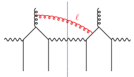
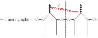
Refer to caption
Refer to caption
Figure 9: Graphical representation of applying the Grammer-Yennie approximation and a Ward identity to the sum of four graphs. The three other graphs required are graph e in figure 5, and the analogues to graphs d and e in which the gluon couples to the quark line at the very right. It is understood that the gqq¯𝑔𝑞¯𝑞g\to q\bar{q} splitting is hard, whereas the gluons are collinear left moving.

For the HH𝐻𝐻HH region we have

CHHΓdsubscript𝐶𝐻𝐻superscriptΓ𝑑\displaystyle C_{HH}\mskip 1.5mu\Gamma^{d} THHCHCΓe+=qf(0)H(2)G(0)subscript𝑇𝐻𝐻subscript𝐶𝐻𝐶superscriptΓlimit-from𝑒subscript𝑞tensor-productsuperscript𝑓0superscript𝐻2superscript𝐺0\displaystyle-T_{HH}\,C_{HC}\mskip 1.5mu\Gamma^{e+}=\int_{q}f^{(0)}\,H^{(2)}\otimes G^{(0)}
[qf(0)Kren(1)H(1)G(0)σ^1(0)σ^2(0)yΦ2(yν)f(0)Kren(1)V(1)(y)G(0)]delimited-[]subscript𝑞tensor-producttensor-productsuperscript𝑓0subscriptsuperscript𝐾1rensuperscript𝐻1superscript𝐺0subscriptsuperscript^𝜎01subscriptsuperscript^𝜎02subscript𝑦tensor-productsuperscriptΦ2𝑦𝜈superscript𝑓0subscriptsuperscript𝐾1rensuperscript𝑉1𝑦superscript𝐺0\displaystyle\quad-\biggl{[}\int_{q}f^{(0)}\otimes K^{(1)}_{\text{ren}}\;H^{(1)}\otimes G^{(0)}-\hat{\sigma}^{(0)}_{1}\hat{\sigma}^{(0)}_{2}\int_{y}\Phi^{2}(y\nu)\,f^{(0)}\otimes K^{(1)}_{\text{ren}}\;V^{(1)}(y)\,G^{(0)}\biggr{]}
σ^1(0)σ^2(0)yΦ2(yν)f(0)V(2)(y)G(0).subscriptsuperscript^𝜎01subscriptsuperscript^𝜎02subscript𝑦superscriptΦ2𝑦𝜈superscript𝑓0superscript𝑉2𝑦superscript𝐺0\displaystyle\quad-\hat{\sigma}^{(0)}_{1}\hat{\sigma}^{(0)}_{2}\int_{y}\Phi^{2}(y\nu)\,f^{(0)}\,V^{(2)}(y)\,G^{(0)}\,. (79)

In the subtraction term for the region HC𝐻𝐶HC, we have an NLO contribution Kren(1)subscriptsuperscript𝐾1renK^{(1)}_{\text{ren}} to the gg𝑔𝑔gg splitting kernel with a gluon coupling to an eikonal line, in analogy to fren(1)subscriptsuperscript𝑓1renf^{(1)}_{\text{ren}} above. Again, this requires summation over several graphs as specified on the l.h.s. In the last line of (5) we have the subtraction term for the region CC𝐶𝐶CC, in which the gluon and the splitting are regarded as collinear, so that no eikonal approximation is made and one obtains an NLO contribution V(2)superscript𝑉2V^{(2)} to the gqq¯𝑔𝑞¯𝑞g\to q\bar{q} splitting kernel. Adding all contributions, we obtain

Γd+(1THH)CHCΓe+superscriptΓ𝑑1subscript𝑇𝐻𝐻subscript𝐶𝐻𝐶superscriptΓlimit-from𝑒\displaystyle\Gamma^{d}+(1-T_{HH})\,C_{HC}\mskip 1.5mu\Gamma^{e+} =q(fren(1)H(1)+f(0)[H(2)Kren(1)H(1)])G(0)absentsubscript𝑞tensor-productsubscriptsuperscript𝑓1rensuperscript𝐻1superscript𝑓0delimited-[]superscript𝐻2subscriptsuperscript𝐾1rensuperscript𝐻1superscript𝐺0\displaystyle=\int_{q}\Bigl{(}f^{(1)}_{\text{ren}}\,H^{(1)}+f^{(0)}\,\bigl{[}H^{(2)}-K^{(1)}_{\text{ren}}\;H^{(1)}\bigr{]}\Bigr{)}\otimes G^{(0)}
σ^1(0)σ^2(0)yΦ2(yν)Fspl,pt(2)(y)Fint,pt(0)(y)subscriptsuperscript^𝜎01subscriptsuperscript^𝜎02subscript𝑦superscriptΦ2𝑦𝜈subscriptsuperscript𝐹2spl,pt𝑦subscriptsuperscript𝐹0int,pt𝑦\displaystyle\quad-\hat{\sigma}^{(0)}_{1}\hat{\sigma}^{(0)}_{2}\int_{y}\Phi^{2}(y\nu)\,F^{(2)}_{\text{spl,pt}}(y)\,F^{(0)}_{\text{int,pt}}(y)
+σ^1(0)σ^2(0)yΦ2(yν)Fspl(2)(y)Fint(0)(y),subscriptsuperscript^𝜎01subscriptsuperscript^𝜎02subscript𝑦superscriptΦ2𝑦𝜈subscriptsuperscript𝐹2spl𝑦subscriptsuperscript𝐹0int𝑦\displaystyle\quad+\hat{\sigma}^{(0)}_{1}\hat{\sigma}^{(0)}_{2}\int_{y}\Phi^{2}(y\nu)\,F^{(2)}_{\text{spl}}(y)\,F^{(0)}_{\text{int}}(y)\,, (80)

where

Fspl,pt(2)(y)subscriptsuperscript𝐹2spl,pt𝑦\displaystyle F^{(2)}_{\text{spl,pt}}(y) =d and e+fren(1)V(1)(y)+f(0)[V(2)(y)Kren(1)V(1)(y)]limit-from𝑑 and 𝑒subscriptsuperscript𝑓1rensuperscript𝑉1𝑦superscript𝑓0delimited-[]superscript𝑉2𝑦subscriptsuperscript𝐾1rensuperscript𝑉1𝑦\displaystyle\;\underset{d\text{ and }e+}{=}\;f^{(1)}_{\text{ren}}\,V^{(1)}(y)+f^{(0)}\bigl{[}V^{(2)}(y)-K^{(1)}_{\text{ren}}\;V^{(1)}(y)\bigr{]} (81)

is a contribution to the perturbative splitting DPD at NLO. The scale dependence of fren(1)subscriptsuperscript𝑓1renf^{(1)}_{\text{ren}} and Kren(1)subscriptsuperscript𝐾1renK^{(1)}_{\text{ren}} cancels in (81), corresponding to the fact that graph 5d and the other ones required for applying the Ward identity do not contribute to the scale evolution of the DPD.

Other NLO graphs.

The discussion of graphs where the extra gluon is exchanged between a right-moving and a left-moving line, such as in figure 5e and f, is more complicated because it involves more momentum regions. Depending on whether the gqq¯𝑔𝑞¯𝑞g\to q\bar{q} splitting is collinear or hard, the extra gluon can be hard (H𝐻H), collinear left moving (L𝐿L), collinear right-moving (R𝑅R), or soft (S𝑆S). In the three latter cases, one can apply the Grammer-Yennie approximation and, after summation over an appropriate set of graphs, apply Ward identities, similarly to the example we have just discussed. This leads to the gluon coupling to eikonal lines, which in regions L𝐿L and R𝑅R are part of the Wilson lines in the operator defining the DPDs, whereas in region S𝑆S they are part of the Wilson lines in the soft factor. For more details we refer to Diehl:2015bca . Our formulation of the DPS cross section in transverse position space is well suited for the treatment of these Wilson lines, which are taken at the same transverse positions as the quark or gluon fields in the DPD definitions. In transverse momentum space, one instead has a more complicated structure with convolution integrals.

6 Double DGLAP evolution

Collinear DPDs F(xi,𝒚;μi)𝐹subscript𝑥𝑖𝒚subscript𝜇𝑖F(x_{i},\boldsymbol{y};\mu_{i}) evolve with μisubscript𝜇𝑖\mu_{i} according to the double DGLAP equations. In the present section, we discuss several aspects of this scale dependence.

6.1 Resummation of large logarithms

As we have seen in section 4.1.2, the 2v1 graph in figure 5a gives rise to a large logarithm log(Q/Λ)𝑄Λ\log(Q/\Lambda) when the cross section is integrated over the transverse boson momenta. This logarithm originates from the gqq¯𝑔𝑞¯𝑞g\to q\bar{q} splitting vertices in the kinematic region of double parton scattering and is correctly reproduced in the DPS cross section, provided that we make a suitable choice of scales.

Radiative corrections to figure 5a give rise to additional large logarithms of DGLAP type. One can expect that these logarithms are correctly resummed to all orders by the DGLAP evolution of the DPDs, provided again that one makes suitable scale choices. In this section we show for explicit examples that this is indeed the case. We will allow for different hard scales Q1,Q2subscript𝑄1subscript𝑄2Q_{1},Q_{2} and set the scales as

μ1subscript𝜇1\displaystyle\mu_{1} =Q1,absentsubscript𝑄1\displaystyle=Q_{1}\,, μ2subscript𝜇2\displaystyle\mu_{2} =Q2,absentsubscript𝑄2\displaystyle=Q_{2}\,, ν𝜈\displaystyle\nu =Qmin,absentsubscript𝑄min\displaystyle=Q_{\text{min}}\,, (82)

where we define

Qminsubscript𝑄min\displaystyle Q_{\text{min}} =min(Q1,Q2).absentsubscript𝑄1subscript𝑄2\displaystyle=\min{(Q_{1},Q_{2})}\,. (83)

Of course, our conclusions regarding large logarithms will not change if (82) is modified by factors of order unity. For definiteness, we will always take a rigid cutoff Φ(u)=Θ(ub0)Φ𝑢Θ𝑢subscript𝑏0\Phi(u)=\Theta(u-b_{0}) in yν𝑦𝜈y\nu. For later use we define the scale

μysubscript𝜇𝑦\displaystyle\mu_{y} =b0y.absentsubscript𝑏0𝑦\displaystyle=\frac{b_{0}}{y}\,. (84)

DGLAP logarithms are generated by loop integrals in regions of strongly ordered transverse momenta. We will compare the logarithms obtained directly from transverse momentum integrals with the ones obtained from evolved DPDs in y𝑦y space.

To set the scene, we start with the lowest-order 2v1 graph in figure 5a. In the DPS region, i.e. when the scale of the gqq¯𝑔𝑞¯𝑞g\to q\bar{q} splittings is much smaller than Q1subscript𝑄1Q_{1} and Q2subscript𝑄2Q_{2}, the behaviour of a splitting vertex is easily recovered from the computation of the splitting DPD. As can be seen from (3.1), a vertex with quark momentum k𝑘k gives a factor 𝒌j/𝒌2superscript𝒌𝑗superscript𝒌2\boldsymbol{k}^{j}/\boldsymbol{k}^{2}, where j𝑗j is a transverse index. The transverse momentum of the splitting vertices must flow through the gauge boson lines. Thus, the two splitting vertices in figure 5a give a combined 1/q121superscriptsubscript𝑞121/q_{1}^{2} behaviour for q1Qminmuch-less-thansubscript𝑞1subscript𝑄minq_{1}\ll Q_{\text{min}}, as is evident in (4.1.2) after angular integration. The integrated cross section is then proportional to

Λ2Qmin2dq12q12=logQmin2Λ2.superscriptsubscriptsuperscriptΛ2superscriptsubscript𝑄min2𝑑superscriptsubscript𝑞12superscriptsubscript𝑞12superscriptsubscript𝑄min2superscriptΛ2\displaystyle\int_{\Lambda^{2}}^{Q_{\text{min}}^{2}}\frac{dq_{1}^{2}}{q_{1}^{2}}=\log\frac{Q_{\text{min}}^{2}}{\Lambda^{2}}\,. (85)

Since the q1subscript𝑞1q_{1} integral is logarithmic, we must include an infrared cutoff ΛΛ\Lambda, which limits the integration to the perturbative region where the preceding analysis is valid. We take here the usual procedure for extracting the leading behaviour of a logarithmic integral ab𝑑kΓ(k)superscriptsubscript𝑎𝑏differential-d𝑘Γ𝑘\int_{a}^{b}dk\;\Gamma(k), approximating the integrand Γ(k)Γ𝑘\Gamma(k) for akbmuch-less-than𝑎𝑘much-less-than𝑏a\ll k\ll b while integrating over the full range akb𝑎𝑘𝑏a\leq k\leq b.

Let us now see how the logarithm (85) arises in the DPS cross section formula. According to the perturbative expressions of the DPDs, Fspl,pt1/y2similar-tosubscript𝐹spl,pt1superscript𝑦2F_{\text{spl,pt}}\sim 1/y^{2} and Fint,ptsubscript𝐹int,ptF_{\text{int,pt}} is y𝑦y independent at leading order in αssubscript𝛼𝑠\alpha_{s}, so that we have

b02/ν2b02/Λ2dy2y2=logQmin2Λ2.superscriptsubscriptsuperscriptsubscript𝑏02superscript𝜈2superscriptsubscript𝑏02superscriptΛ2𝑑superscript𝑦2superscript𝑦2superscriptsubscript𝑄min2superscriptΛ2\displaystyle\int_{b_{0}^{2}/\nu^{2}}^{b_{0}^{2}/\Lambda^{2}}\frac{dy^{2}}{y^{2}}=\log\frac{Q_{\text{min}}^{2}}{\Lambda^{2}}\,. (86)

With our choice for the infrared cutoff on y𝑦y, the expressions (85) and (86) agree including their overall normalisation.
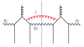
Refer to caption
Refer to caption
Refer to caption
Figure 10: Radiative corrections to the hard scattering graph in figure 5a that give rise to DGLAP logarithms.

Now consider the NLO graph in figure 10a. We route the gluon momentum \ell back through the boson line with momentum q2subscript𝑞2q_{2}, so that \ell flows through exactly two quark propagators. In the strongly ordered region

ΛΛ\displaystyle\Lambda q1Q1,much-less-thanabsentsubscript𝑞1much-less-thansubscript𝑄1\displaystyle\ll q_{1}\ll Q_{1}\,, q1subscript𝑞1\displaystyle q_{1} Q2much-less-thanabsentmuch-less-thansubscript𝑄2\displaystyle\ll\ell\ll Q_{2} (87)

the graph has the same DPS logarithm as the leading-order result, whilst developing an additional logarithm from the integral 𝑑2/2differential-dsuperscript2superscript2\int d\ell^{2}/\ell^{2}, as is familiar from similar gluon emission graphs in hard scattering processes. In the case Q2<Q1subscript𝑄2subscript𝑄1Q_{2}<Q_{1} this gives

Λ2Q22dq12q12q12Q22d22superscriptsubscriptsuperscriptΛ2superscriptsubscript𝑄22𝑑superscriptsubscript𝑞12superscriptsubscript𝑞12superscriptsubscriptsuperscriptsubscript𝑞12superscriptsubscript𝑄22𝑑superscript2superscript2\displaystyle\int_{\Lambda^{2}}^{Q_{2}^{2}}\frac{dq_{1}^{2}}{q_{1}^{2}}\int_{q_{1}^{2}}^{Q_{2}^{2}}\frac{d\ell^{2}}{\ell^{2}} =12log2Q22Λ2=12log2Qmin2Λ2,absent12superscript2superscriptsubscript𝑄22superscriptΛ212superscript2superscriptsubscript𝑄min2superscriptΛ2\displaystyle=\frac{1}{2}\log^{2}\frac{Q_{2}^{2}}{\Lambda^{2}}=\frac{1}{2}\log^{2}\frac{Q_{\text{min}}^{2}}{\Lambda^{2}}\,, (88)

whereas for Q1<Q2subscript𝑄1subscript𝑄2Q_{1}<Q_{2} we have

Λ2Q12dq12q12q12Q22d22superscriptsubscriptsuperscriptΛ2superscriptsubscript𝑄12𝑑superscriptsubscript𝑞12superscriptsubscript𝑞12superscriptsubscriptsuperscriptsubscript𝑞12superscriptsubscript𝑄22𝑑superscript2superscript2\displaystyle\int_{\Lambda^{2}}^{Q_{1}^{2}}\frac{dq_{1}^{2}}{q_{1}^{2}}\int_{q_{1}^{2}}^{Q_{2}^{2}}\frac{d\ell^{2}}{\ell^{2}} =12[log2Q22Λ2log2Q22Q12]=12logQmin2Λ2[logQmin2Λ2+2logQ22Q12].absent12delimited-[]superscript2superscriptsubscript𝑄22superscriptΛ2superscript2superscriptsubscript𝑄22superscriptsubscript𝑄1212superscriptsubscript𝑄min2superscriptΛ2delimited-[]superscriptsubscript𝑄min2superscriptΛ22superscriptsubscript𝑄22superscriptsubscript𝑄12\displaystyle=\frac{1}{2}\,\biggl{[}\log^{2}\frac{Q_{2}^{2}}{\Lambda^{2}}-\log^{2}\frac{Q_{2}^{2}}{Q_{1}^{2}}\biggr{]}=\frac{1}{2}\log\frac{Q_{\text{min}}^{2}}{\Lambda^{2}}\biggl{[}\log\frac{Q_{\text{min}}^{2}}{\Lambda^{2}}+2\log\frac{Q_{2}^{2}}{Q_{1}^{2}}\biggr{]}\,. (89)

In both cases, we have an additional logarithm log(Qmin2/Λ2)superscriptsubscript𝑄min2superscriptΛ2\log(Q_{\text{min}}^{2}/\Lambda^{2}) compared with the lowest-order result. If Q1Q2much-less-thansubscript𝑄1subscript𝑄2Q_{1}\ll Q_{2}, then the logarithm of the ratio Q2/Q1subscript𝑄2subscript𝑄1Q_{2}/Q_{1} is also large.

Let us compare these results with the 2v1 part of the DPS cross section formula when we take into account evolution of the splitting DPD. Focusing on the dependence on y𝑦y and μ𝜇\mu, we can write

Fspl,pt(xi,𝒚;μy,μy)subscript𝐹spl,ptsubscript𝑥𝑖𝒚subscript𝜇𝑦subscript𝜇𝑦\displaystyle F_{\text{spl,pt}}(x_{i},\boldsymbol{y};\mu_{y},\mu_{y}) 1y2αs(μy)g(x1+x2;μy)proportional-toabsent1superscript𝑦2subscript𝛼𝑠subscript𝜇𝑦𝑔subscript𝑥1subscript𝑥2subscript𝜇𝑦\displaystyle\propto\,\frac{1}{y^{2}}\,\alpha_{s}(\mu_{y})\,g(x_{1}+x_{2};\mu_{y}) (90)

at leading order, where the choice of scale μysubscript𝜇𝑦\mu_{y} ensures that there are no large logarithms of yμ𝑦𝜇y\mu in the higher-order corrections. This should be evolved to Fspl,pt(xi,𝒚;μ1,μ2)subscript𝐹spl,ptsubscript𝑥𝑖𝒚subscript𝜇1subscript𝜇2F_{\text{spl,pt}}(x_{i},\boldsymbol{y};\mu_{1},\mu_{2}) in the cross section. In (90) there is a logarithmic dependence on y𝑦y from the running of αssubscript𝛼𝑠\alpha_{s} and from the scale dependence of the gluon density. Graph 10a does not contribute to either of these, so that the corresponding dependence should not be taken into account here. Rather, the DGLAP logarithm of graph 10a corresponds to the evolution of (90) from μysubscript𝜇𝑦\mu_{y} to μ2subscript𝜇2\mu_{2}, which gives a factor proportional to αslog(μ22/μy2)subscript𝛼𝑠superscriptsubscript𝜇22superscriptsubscript𝜇𝑦2\alpha_{s}\log(\mu_{2}^{2}/\mu_{y}^{2}). The relevant y𝑦y integral in the DPD cross section thus is

b02/ν2b02/Λ2dy2y2logy2μ22b02superscriptsubscriptsuperscriptsubscript𝑏02superscript𝜈2superscriptsubscript𝑏02superscriptΛ2𝑑superscript𝑦2superscript𝑦2superscript𝑦2superscriptsubscript𝜇22superscriptsubscript𝑏02\displaystyle\int_{b_{0}^{2}/\nu^{2}}^{b_{0}^{2}/\Lambda^{2}}\frac{dy^{2}}{y^{2}}\,\log\frac{y^{2}\mu_{2}^{2}}{b_{0}^{2}} =12[log2Q22Λ2log2Q22Qmin2],absent12delimited-[]superscript2superscriptsubscript𝑄22superscriptΛ2superscript2superscriptsubscript𝑄22superscriptsubscript𝑄min2\displaystyle=\frac{1}{2}\,\biggl{[}\log^{2}\frac{Q_{2}^{2}}{\Lambda^{2}}-\log^{2}\frac{Q_{2}^{2}}{Q_{\text{min}}^{2}}\biggr{]}\,, (91)

where we have used the scale choice in (82). This agrees with both (88) and (89).

Note the ease with which (91) is obtained in y𝑦y space, compared with the detailed considerations leading to (88) and (89). We see that with evolved DPDs in σDPSsubscript𝜎DPS\sigma_{\text{DPS}} one includes higher order logarithms while using tree-level partonic cross sections. Treating the 2v1 graphs fully within the collinear twist-four formalism would require the explicit inclusion of the higher-order graphs.

Whereas in the previous example, the gluon is emitted close to the splitting vertices, the opposite is true for the graphs in figure 10b and c. For figure 10b the region generating two large logarithms is

ΛΛ\displaystyle\Lambda q1Qmin,much-less-thanabsentsubscript𝑞1much-less-thansubscript𝑄min\displaystyle\ll q_{1}\ll Q_{\text{min}}\,, ΛΛ\displaystyle\Lambda Q2,much-less-thanabsentmuch-less-thansubscript𝑄2\displaystyle\ll\ell\ll Q_{2}\,, (92)

which gives

Λ2Qmin2dq12q12Λ2Q22d22superscriptsubscriptsuperscriptΛ2superscriptsubscript𝑄min2𝑑superscriptsubscript𝑞12superscriptsubscript𝑞12superscriptsubscriptsuperscriptΛ2superscriptsubscript𝑄22𝑑superscript2superscript2\displaystyle\int_{\Lambda^{2}}^{Q_{\text{min}}^{2}}\frac{dq_{1}^{2}}{q_{1}^{2}}\int_{\Lambda^{2}}^{Q_{2}^{2}}\frac{d\ell^{2}}{\ell^{2}} =logQmin2Λ2logQ22Λ2.absentsuperscriptsubscript𝑄min2superscriptΛ2superscriptsubscript𝑄22superscriptΛ2\displaystyle=\log\frac{Q_{\text{min}}^{2}}{\Lambda^{2}}\,\log\frac{Q_{2}^{2}}{\Lambda^{2}}\,. (93)

To see how these logarithms arise from the evolution of Fint,ptsubscript𝐹int,ptF_{\text{int,pt}}, we use the short-distance expansion

Fint,pt(x1,x2,𝒚;μy,μy)subscript𝐹int,ptsubscript𝑥1subscript𝑥2𝒚subscript𝜇𝑦subscript𝜇𝑦\displaystyle F_{\text{int,pt}}(x_{1},x_{2},\boldsymbol{y};\mu_{y},\mu_{y}) =G(x1,x2,x2,x1;μy)absent𝐺subscript𝑥1subscript𝑥2subscript𝑥2subscript𝑥1subscript𝜇𝑦\displaystyle=G(x_{1},x_{2},x_{2},x_{1};\mu_{y}) (94)

at leading order, which we evaluate at scale μysubscript𝜇𝑦\mu_{y} to avoid large logarithms of yμ𝑦𝜇y\mu in the higher-order corrections, as we did for Fspl,ptsubscript𝐹spl,ptF_{\text{spl,pt}} in (90). Graph 10b contributes to the scale evolution of G𝐺G, where at leading order it gives αslog(μy2/Λ2)subscript𝛼𝑠superscriptsubscript𝜇𝑦2superscriptΛ2\alpha_{s}\log(\mu_{y}^{2}/\Lambda^{2}) when evolution is started from the generic soft scale Λ2superscriptΛ2\Lambda^{2}. The graph also contributes to the evolution of Fint,ptsubscript𝐹int,ptF_{\text{int,pt}} from μysubscript𝜇𝑦\mu_{y} to μ2subscript𝜇2\mu_{2}, where it gives αslog(μ22/μy2)subscript𝛼𝑠superscriptsubscript𝜇22superscriptsubscript𝜇𝑦2\alpha_{s}\log(\mu_{2}^{2}/\mu_{y}^{2}). The two effects add up to a factor αslog(μ2/Λ2)subscript𝛼𝑠subscript𝜇2superscriptΛ2\alpha_{s}\log(\mu_{2}/\Lambda^{2}). In the DPS cross section we thus have

b02/ν2b02/Λ2dy2y2logμ22Λ2superscriptsubscriptsuperscriptsubscript𝑏02superscript𝜈2superscriptsubscript𝑏02superscriptΛ2𝑑superscript𝑦2superscript𝑦2superscriptsubscript𝜇22superscriptΛ2\displaystyle\int_{b_{0}^{2}/\nu^{2}}^{b_{0}^{2}/\Lambda^{2}}\frac{dy^{2}}{y^{2}}\,\log\frac{\mu_{2}^{2}}{\Lambda^{2}} =logQmin2Λ2logQ22Λ2absentsuperscriptsubscript𝑄min2superscriptΛ2superscriptsubscript𝑄22superscriptΛ2\displaystyle=\log\frac{Q_{\text{min}}^{2}}{\Lambda^{2}}\,\log\frac{Q_{2}^{2}}{\Lambda^{2}} (95)

in agreement with (93).

The graph in figure 10c also has a region where DGLAP logarithms are generated, as was already discussed in Gaunt:2012dd . We route the loop momentum \ell through two quark lines at one of the two gqq¯𝑔𝑞¯𝑞g\to q\bar{q} splitting vertices. In the strongly ordered region

ΛΛ\displaystyle\Lambda q1Qminmuch-less-thanabsentmuch-less-thansubscript𝑞1much-less-thansubscript𝑄min\displaystyle\ll\ell\ll q_{1}\ll Q_{\text{min}} (96)

the two lower fermion lines to which the gluon couples have virtualities of order 2superscript2\ell^{2}, whereas both splitting vertices have virtualities of order q12q22superscriptsubscript𝑞12superscriptsubscript𝑞22q_{1}^{2}\approx q_{2}^{2}. This gives 777Note that in equation (3.13) of Gaunt:2012dd a factor 1/2121/2 is missing on the r.h.s.

Λ2Qmin2dq12q12Λ2q12d22superscriptsubscriptsuperscriptΛ2superscriptsubscript𝑄min2𝑑superscriptsubscript𝑞12superscriptsubscript𝑞12superscriptsubscriptsuperscriptΛ2superscriptsubscript𝑞12𝑑superscript2superscript2\displaystyle\int_{\Lambda^{2}}^{Q_{\text{min}}^{2}}\frac{dq_{1}^{2}}{q_{1}^{2}}\int_{\Lambda^{2}}^{q_{1}^{2}}\frac{d\ell^{2}}{\ell^{2}} =12log2Qmin2Λ2.absent12superscript2superscriptsubscript𝑄min2superscriptΛ2\displaystyle=\frac{1}{2}\log^{2}\frac{Q_{\text{min}}^{2}}{\Lambda^{2}}\,. (97)

Just as graph 10b, graph c contributes to the evolution of G𝐺G in (94), giving a factor αslog(μy2/Λ2)subscript𝛼𝑠superscriptsubscript𝜇𝑦2superscriptΛ2\alpha_{s}\log(\mu_{y}^{2}/\Lambda^{2}) at leading order. There is however no contribution to the evolution of Fint,ptsubscript𝐹int,ptF_{\text{int,pt}} from μysubscript𝜇𝑦\mu_{y} to μ2subscript𝜇2\mu_{2} from this graph, so that in the cross section we have

b02/ν2b02/Λ2dy2y2logb02Λ2y2superscriptsubscriptsuperscriptsubscript𝑏02superscript𝜈2superscriptsubscript𝑏02superscriptΛ2𝑑superscript𝑦2superscript𝑦2superscriptsubscript𝑏02superscriptΛ2superscript𝑦2\displaystyle\int_{b_{0}^{2}/\nu^{2}}^{b_{0}^{2}/\Lambda^{2}}\frac{dy^{2}}{y^{2}}\,\log\frac{b_{0}^{2}}{\Lambda^{2}y^{2}} =12log2Qmin2Λ2,absent12superscript2superscriptsubscript𝑄min2superscriptΛ2\displaystyle=\frac{1}{2}\log^{2}\frac{Q_{\text{min}}^{2}}{\Lambda^{2}}\,, (98)

which again reproduces the result (97) obtained in momentum space, including the overall factor.

A fully analogous discussion can be given for the graph in figure 5b. One finds the same type of DGLAP logarithms as in (97), which is again reproduced correctly in the DPS cross section formula. Note that in this case the additional gluon is a virtual correction rather than emitted into the final state – a somewhat unusual situation in the context of DGLAP logarithms.

In conclusion, higher-order graphs with strong ordering of transverse momenta produce DGLAP type logarithms in 2v1 graphs, which can depend on Qmin/Λsubscript𝑄minΛQ_{\text{min}}/\Lambda or Q2/Q1subscript𝑄2subscript𝑄1Q_{2}/Q_{1}. Our expression for the regularised DPS cross section correctly reproduces these logarithms if we make an adequate choice of DPDs and scales. Specifically, we must

  • use DPDs that have the correct short-distance behaviour, as discussed in section 3.3. Fixed-order perturbative results for this behaviour can be used reliably at scales of order μysubscript𝜇𝑦\mu_{y}, as in (90) and (94).

  • take scales μ1,μ2subscript𝜇1subscript𝜇2\mu_{1},\mu_{2} and ν𝜈\nu in σDPSsubscript𝜎DPS\sigma_{\text{DPS}} as specified in (82), with possible modifications by factors of order unity.

The situation is quite different for 1v1 graphs. In the DPS region

q1k±Qminmuch-less-thansubscript𝑞1subscript𝑘plus-or-minusmuch-less-thansubscript𝑄min\displaystyle q_{1}\ll k_{\pm}\ll Q_{\text{min}} (99)

the double box in figure 11a develops a squared DPS logarithm in dσ/dq12𝑑𝜎𝑑superscriptsubscript𝑞12d\sigma/dq_{1}^{2},

q12Qmin2dk+2k+2q12Qmin2dk2k2superscriptsubscriptsuperscriptsubscript𝑞12superscriptsubscript𝑄min2𝑑superscriptsubscript𝑘2superscriptsubscript𝑘2superscriptsubscriptsuperscriptsubscript𝑞12superscriptsubscript𝑄min2𝑑superscriptsubscript𝑘2superscriptsubscript𝑘2\displaystyle\int_{q_{1}^{2}}^{Q_{\text{min}}^{2}}\frac{dk_{+}^{2}}{k_{+}^{2}}\,\int_{q_{1}^{2}}^{Q_{\text{min}}^{2}}\frac{dk_{-}^{2}}{k_{-}^{2}} =log2Qmin2q12absentsuperscript2superscriptsubscript𝑄min2superscriptsubscript𝑞12\displaystyle=\log^{2}\frac{Q_{\text{min}}^{2}}{q_{1}^{2}} (100)

which disappears however when one integrates over q1subscript𝑞1q_{1} up to Qminsubscript𝑄minQ_{\text{min}}. This is inevitable since the integrated 1v1 cross section depends on a single dimensionful quantity Qminsubscript𝑄minQ_{\text{min}} and hence cannot have any large logarithm. An infrared cutoff ΛΛ\Lambda in the q1subscript𝑞1q_{1} integration does not play any role here since the cross section is dominated by large q1Qminsimilar-tosubscript𝑞1subscript𝑄minq_{1}\sim Q_{\text{min}}, where strong ordering as in (99) is not possible.

One finds that the higher-order graph in figure 11b does have a DGLAP logarithm in the strong-ordering regime

q1k±much-less-thansubscript𝑞1subscript𝑘plus-or-minus\displaystyle q_{1}\ll k_{\pm} Q1,much-less-thanabsentsubscript𝑄1\displaystyle\ll Q_{1}\,, k±subscript𝑘plus-or-minus\displaystyle k_{\pm} Q2,much-less-thanabsentmuch-less-thansubscript𝑄2\displaystyle\ll\ell\ll Q_{2}\,, (101)

due to the additional loop integral 𝑑2/2differential-dsuperscript2superscript2\int d\ell^{2}/\ell^{2}. But the region (101) gives only a power suppressed contribution to the cross section integrated over q1subscript𝑞1q_{1}, where DPS kinematics is not dominant.888This point was overlooked in the discussion of DGLAP logarithms in Diehl:2016khr ; Diehl:2016rqr .
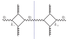
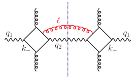
Refer to caption
Refer to caption
Figure 11: (a) Hard scattering part of the double box graph. (b) Higher-order correction giving rise to a large DGLAP logarithm in the DPS region.

There is an exception to the statement just made. If at least one of the momentum fractions x1,x2subscript𝑥1subscript𝑥2x_{1},x_{2} is very small and the corresponding scale μ1,μ2subscript𝜇1subscript𝜇2\mu_{1},\mu_{2} is sufficiently large, then the evolution of Fspl,ptsubscript𝐹spl,ptF_{\text{spl,pt}} from μysubscript𝜇𝑦\mu_{y} to μ1subscript𝜇1\mu_{1}, μ2subscript𝜇2\mu_{2} can significantly flatten the 1/y21superscript𝑦21/y^{2} behaviour of the initial condition (90). The underlying physics is radiation of soft gluons, which strongly enhances parton distributions at low x𝑥x, as is well known from the evolution of ordinary PDFs. The enhancement by evolution of Fspl,ptsubscript𝐹spl,ptF_{\text{spl,pt}} increases with the distance between μysubscript𝜇𝑦\mu_{y} and μ1,μ2subscript𝜇1subscript𝜇2\mu_{1},\mu_{2}, i.e. it increases with y𝑦y. In the 1v1 (and also the 2v1) contribution to the DPS cross section, this enhances the importance of the region y1/Qmuch-greater-than𝑦1𝑄y\gg 1/Q, where the DPS approximation is valid. In this region, the evolution of the DPDs correctly describes the DGLAP logarithms generated by graphs like the one in figure 11b. In the numerical studies presented in section 9.2, we find that this happens for Fggsubscript𝐹𝑔𝑔F_{gg}, Fqgsubscript𝐹𝑞𝑔F_{qg} and Fq¯gsubscript𝐹¯𝑞𝑔F_{\bar{q}g}, as well as for Fqq¯subscript𝐹𝑞¯𝑞F_{q\bar{q}} when one momentum fraction is much smaller than the other.

6.2 Dependence on the cutoff scale

As already discussed in section 4.1, our formalism relies on the fact that in the region of small y1/Qsimilar-to𝑦1𝑄y\sim 1/Q the subtraction terms in the cross section (45) cancel against the DPS contribution, up to corrections that are beyond the accuracy of the calculation. Such corrections include higher-order terms in αssubscript𝛼𝑠\alpha_{s}, whose parametric size we now investigate.

Let Ffo(xi,𝒚;μ)subscript𝐹fosubscript𝑥𝑖𝒚𝜇F_{\text{fo}}(x_{i},\boldsymbol{y};\mu) denote the short distance approximation of a DPD, computed in fixed-order perturbation theory. It depends on μ𝜇\mu via the scales of αssubscript𝛼𝑠\alpha_{s} and of PDFs or twist-four distributions (and at higher orders also via powers of log(yμ)𝑦𝜇\log(y\mu) in the splitting kernels). In the cross section, this fixed-order approximation is used in two different ways:

  1. 1.

    For the small-y𝑦y limit of the DPDs used in the DPS cross section, σDPSsubscript𝜎DPS\sigma_{\text{DPS}}, one takes Ffo(xi,𝒚;μy)subscript𝐹fosubscript𝑥𝑖𝒚subscript𝜇𝑦F_{\text{fo}}(x_{i},\boldsymbol{y};\mu_{y}) as initial condition and evolves it to the scales μ1Q1similar-tosubscript𝜇1subscript𝑄1\mu_{1}\sim Q_{1} and μ2Q2similar-tosubscript𝜇2subscript𝑄2\mu_{2}\sim Q_{2} of the two hard scatters.

  2. 2.

    In the subtraction terms, σ1v1,ptsubscript𝜎1v1,pt\sigma_{\text{1v1,pt}} and σ2v1,ptsubscript𝜎2v1,pt\sigma_{\text{2v1,pt}}, one takes Ffo(xi,𝒚;μh)subscript𝐹fosubscript𝑥𝑖𝒚subscript𝜇F_{\text{fo}}(x_{i},\boldsymbol{y};\mu_{h}) evaluated at the same scale μhsubscript𝜇\mu_{h} that is used in the hard scattering terms, σSPSsubscript𝜎SPS\sigma_{\text{SPS}} or σtw4subscript𝜎tw4\sigma_{\text{tw4}}, so as to cancel the contribution from the region y1/Qmuch-greater-than𝑦1𝑄y\gg 1/Q order by order in perturbation theory.

The scale μhsubscript𝜇\mu_{h} may be a combination of Q1subscript𝑄1Q_{1} or Q2subscript𝑄2Q_{2} or an independent third scale. For now we assume that αsL1much-less-thansubscript𝛼𝑠𝐿1\alpha_{s}\mskip 1.5muL\ll 1, where

L𝐿\displaystyle L =max{|log(Q2/Q1)|,|log(μh/Q1)|,|log(μh/Q2)|}.absentsubscript𝑄2subscript𝑄1subscript𝜇subscript𝑄1subscript𝜇subscript𝑄2\displaystyle=\max\mskip 1.5mu\bigl{\{}|\log(Q_{2}/Q_{1})|\mskip 1.5mu,|\log(\mu_{h}/Q_{1})|\mskip 1.5mu,|\log(\mu_{h}/Q_{2})|\mskip 1.5mu\bigr{\}}\,. (102)

The case where this is not satisfied because the hard scales are widely different is discussed in the following subsection.

Consider now a calculation at NkLO (k=0𝑘0k=0 for LO), using DPDs evolved with NkLO kernels P𝑃P and NkLO expressions for the DPS subprocess cross sections σ^1,2subscript^𝜎12\hat{\sigma}_{1,2} and the short-distance approximations Ffosubscript𝐹fo\smash{F_{\text{fo}}}. We have

ddlogμ12σ^1+σ^1x1P+σ^1x¯1P𝑑𝑑superscriptsubscript𝜇12subscript^𝜎1subscript^𝜎1subscript𝑥1tensor-product𝑃subscript^𝜎1subscript¯𝑥1tensor-product𝑃\displaystyle\frac{d}{d\log\mu_{1}^{2}}\,\hat{\sigma}_{1}+\hat{\sigma}_{1}\underset{x_{1}}{\otimes}P+\hat{\sigma}_{1}\underset{\bar{x}_{1}}{\otimes}P =𝒪(αsk+1logk(μ1/Q1))×σ^1absent𝒪superscriptsubscript𝛼𝑠𝑘1superscript𝑘subscript𝜇1subscript𝑄1subscript^𝜎1\displaystyle=\mathcal{O}\bigl{(}\alpha_{s}^{k+1}\log^{k}(\mu_{1}/Q_{1})\bigr{)}\times\hat{\sigma}_{1} (103)

and its analogue for σ^2subscript^𝜎2\hat{\sigma}_{2}. Here tensor-product\otimes denotes the usual Mellin convolution for the indicated variable, and we omit labels and sums for parton species. To understand (103) we observe that the l.h.s. would be exactly zero if σ^1subscript^𝜎1\hat{\sigma}_{1} and P𝑃P were calculated to all orders; the convolution of σ^1subscript^𝜎1\hat{\sigma}_{1} with the relevant parton densities would then be μ1subscript𝜇1\mu_{1} independent. With NkLO truncations on the l.h.s., the first term beyond the accuracy of the calculation is of order αsk+1σ^1superscriptsubscript𝛼𝑠𝑘1subscript^𝜎1\alpha_{s}^{k+1}\mskip 1.5mu\hat{\sigma}_{1}. Furthermore, the highest power of log(μ1/Q1)subscript𝜇1subscript𝑄1\log(\mu_{1}/Q_{1}) in σ^1subscript^𝜎1\hat{\sigma}_{1} is k𝑘k according to the general pattern for logarithms related with the renormalisation or factorisation scale. In a similar fashion we can derive

ddlogμ2Fspl,fo(xi,𝒚;μ)𝑑𝑑superscript𝜇2subscript𝐹spl,fosubscript𝑥𝑖𝒚𝜇\displaystyle\frac{d}{d\log\mu^{2}}\,F_{\text{spl,fo}}(x_{i},\boldsymbol{y};\mu) =Px1Fspl,fo(𝒚;μ)+Px2Fspl,fo(𝒚;μ)absent𝑃subscript𝑥1tensor-productsubscript𝐹spl,fo𝒚𝜇𝑃subscript𝑥2tensor-productsubscript𝐹spl,fo𝒚𝜇\displaystyle=P\underset{x_{1}}{\otimes}F_{\text{spl,fo}}(\boldsymbol{y};\mu)+P\underset{x_{2}}{\otimes}F_{\text{spl,fo}}(\boldsymbol{y};\mu)
+𝒪(αsk+1logk(yμ))×Fspl,fo(𝒚;μ),𝒪superscriptsubscript𝛼𝑠𝑘1superscript𝑘𝑦𝜇subscript𝐹spl,fo𝒚𝜇\displaystyle\quad+\mathcal{O}\bigl{(}\alpha_{s}^{k+1}\log^{k}(y\mu)\bigr{)}\times F_{\text{spl,fo}}(\boldsymbol{y};\mu)\,, (104)

using that k𝑘k is the highest power of log(yμ)𝑦𝜇\log(y\mu) in the NkLO approximation, according to (27). Finally, it is easy to see that for a quantity satisfying

ddlogμ2S(μ)𝑑𝑑superscript𝜇2𝑆𝜇\displaystyle\frac{d}{d\log\mu^{2}}\,S(\mu) =𝒪(αsk+1logk(μ/μ0))×S(μ)absent𝒪superscriptsubscript𝛼𝑠𝑘1superscript𝑘𝜇subscript𝜇0𝑆𝜇\displaystyle=\mathcal{O}\bigl{(}\alpha_{s}^{k+1}\log^{k}(\mu/\mu_{0})\bigr{)}\times S(\mu) (105)

one has

S(μb)S(μa)𝑆subscript𝜇𝑏𝑆subscript𝜇𝑎\displaystyle S(\mu_{b})-S(\mu_{a}) =𝒪(αsk+1logk+1(μa/μ0),αsk+1logk+1(μb/μ0))×S(μa),absent𝒪superscriptsubscript𝛼𝑠𝑘1superscript𝑘1subscript𝜇𝑎subscript𝜇0superscriptsubscript𝛼𝑠𝑘1superscript𝑘1subscript𝜇𝑏subscript𝜇0𝑆subscript𝜇𝑎\displaystyle=\mathcal{O}\bigl{(}\alpha_{s}^{k+1}\log^{k+1}(\mu_{a}/\mu_{0}),\alpha_{s}^{k+1}\log^{k+1}(\mu_{b}/\mu_{0})\bigr{)}\times S(\mu_{a})\,, (106)

where the integration of the differential equation (105) between μasubscript𝜇𝑎\mu_{a} and μbsubscript𝜇𝑏\mu_{b} gives an extra logarithm on the r.h.s. We thus obtain for the small-y𝑦y contribution to the 1v1 cross section

[σ1v1]y1/Q=σ^1(μ1)σ^2(μ2)y1/Qd2𝒚Fspl,pt(𝒚;μ1,μ2)Fspl,pt(𝒚;μ1,μ2)subscriptdelimited-[]subscript𝜎1v1similar-to𝑦1𝑄tensor-producttensor-productsubscript^𝜎1subscript𝜇1subscript^𝜎2subscript𝜇2subscriptsimilar-to𝑦1𝑄superscript𝑑2𝒚subscript𝐹spl,pt𝒚subscript𝜇1subscript𝜇2subscript𝐹spl,pt𝒚subscript𝜇1subscript𝜇2\displaystyle\bigl{[}\sigma_{\text{1v1}}\bigr{]}_{y\sim 1/Q}=\hat{\sigma}_{1}(\mu_{1})\otimes\hat{\sigma}_{2}(\mu_{2})\otimes\!\!\int\limits_{y\sim 1/Q}\!\!\!d^{2}\boldsymbol{y}\;F_{\text{spl,pt}}(\boldsymbol{y};\mu_{1},\mu_{2})\,F_{\text{spl,pt}}(\boldsymbol{y};\mu_{1},\mu_{2})
=y1/Qd2𝒚σ^1(μy)σ^2(μy)Fspl,fo(𝒚;μy)Fspl,fo(𝒚;μy)absentsubscriptsimilar-to𝑦1𝑄tensor-producttensor-productsuperscript𝑑2𝒚subscript^𝜎1subscript𝜇𝑦subscript^𝜎2subscript𝜇𝑦subscript𝐹spl,fo𝒚subscript𝜇𝑦subscript𝐹spl,fo𝒚subscript𝜇𝑦\displaystyle\quad=\int\limits_{y\sim 1/Q}\!\!\!d^{2}\boldsymbol{y}\;\hat{\sigma}_{1}(\mu_{y})\otimes\hat{\sigma}_{2}(\mu_{y})\otimes F_{\text{spl,fo}}(\boldsymbol{y};\mu_{y})\,F_{\text{spl,fo}}(\boldsymbol{y};\mu_{y})
×[1+𝒪(αsk+1logk+1(Q1/μy),αsk+1logk+1(Q2/μy))]absentdelimited-[]1𝒪superscriptsubscript𝛼𝑠𝑘1superscript𝑘1subscript𝑄1subscript𝜇𝑦superscriptsubscript𝛼𝑠𝑘1superscript𝑘1subscript𝑄2subscript𝜇𝑦\displaystyle\qquad\times\Bigl{[}1+\mathcal{O}\bigl{(}\alpha_{s}^{k+1}\log^{k+1}(Q_{1}/\mu_{y}),\,\alpha_{s}^{k+1}\log^{k+1}(Q_{2}/\mu_{y})\bigr{)}\Bigr{]}
=σ^1(μh)σ^2(μh)y1/Qd2𝒚Fspl,fo(𝒚;μh)Fspl,fo(𝒚;μh)absenttensor-producttensor-productsubscript^𝜎1subscript𝜇subscript^𝜎2subscript𝜇subscriptsimilar-to𝑦1𝑄superscript𝑑2𝒚subscript𝐹spl,fo𝒚subscript𝜇subscript𝐹spl,fo𝒚subscript𝜇\displaystyle\quad=\hat{\sigma}_{1}(\mu_{h})\otimes\hat{\sigma}_{2}(\mu_{h})\otimes\!\!\int\limits_{y\sim 1/Q}\!\!\!d^{2}\boldsymbol{y}\;F_{\text{spl,fo}}(\boldsymbol{y};\mu_{h})\,F_{\text{spl,fo}}(\boldsymbol{y};\mu_{h})
×[1+𝒪(αsk+1logk+1(yμh),αsk+1logk+1(yQ1),αsk+1logk+1(yQ2))],absentdelimited-[]1𝒪superscriptsubscript𝛼𝑠𝑘1superscript𝑘1𝑦subscript𝜇superscriptsubscript𝛼𝑠𝑘1superscript𝑘1𝑦subscript𝑄1superscriptsubscript𝛼𝑠𝑘1superscript𝑘1𝑦subscript𝑄2\displaystyle\qquad\times\Bigl{[}1+\mathcal{O}\bigl{(}\alpha_{s}^{k+1}\log^{k+1}(y\mu_{h}),\,\alpha_{s}^{k+1}\log^{k+1}(y\mskip 1.5muQ_{1}),\,\alpha_{s}^{k+1}\log^{k+1}(y\mskip 1.5muQ_{2})\bigr{)}\Bigr{]}\,, (107)

using our initial condition Fspl,pt=Fspl,fosubscript𝐹spl,ptsubscript𝐹spl,foF_{\text{spl,pt}}=F_{\text{spl,fo}} at scale μysubscript𝜇𝑦\mu_{y}. The longitudinal momentum arguments and convolutions are as in (2). The first line of the last expression in (6.2) is just the double counting subtraction term. We thus find

[σ1v1σ1v1,pt]y1/Qsubscriptdelimited-[]subscript𝜎1v1subscript𝜎1v1,ptsimilar-to𝑦1𝑄\displaystyle\bigl{[}\sigma_{\text{1v1}}-\sigma_{\text{1v1,pt}}\bigr{]}_{y\sim 1/Q} =[σ1v1,pt]y1/Q×𝒪(αsk+1Lk+1)absentsubscriptdelimited-[]subscript𝜎1v1,ptsimilar-to𝑦1𝑄𝒪superscriptsubscript𝛼𝑠𝑘1superscript𝐿𝑘1\displaystyle=\bigl{[}\sigma_{\text{1v1,pt}}\bigr{]}_{y\sim 1/Q}\,\times\mathcal{O}\bigl{(}\alpha_{s}^{k+1}L^{k+1}\bigr{)}
=[σSPSσ1v1,pt]×𝒪(αsk+1Lk+1).absentdelimited-[]subscript𝜎SPSsubscript𝜎1v1,pt𝒪superscriptsubscript𝛼𝑠𝑘1superscript𝐿𝑘1\displaystyle=\bigl{[}\sigma_{\text{SPS}}-\sigma_{\text{1v1,pt}}\bigr{]}\,\times\mathcal{O}\bigl{(}\alpha_{s}^{k+1}L^{k+1}\bigr{)}\,. (108)

with L𝐿L defined in (102). In the second step we have used that the full SPS cross section is of the same order of magnitude as the DPS subtraction term, regarding its power behaviour in Q2superscript𝑄2Q^{2} as well as the relevant coupling constants and PDFs. In full analogy one can derive

[σ2v1σ2v1,pt]y1/Qsubscriptdelimited-[]subscript𝜎2v1subscript𝜎2v1,ptsimilar-to𝑦1𝑄\displaystyle\bigl{[}\sigma_{\text{2v1}}-\sigma_{\text{2v1,pt}}\bigr{]}_{y\sim 1/Q} =[σ2v1,pt]y1/Q×𝒪(αsk+1Lk+1)absentsubscriptdelimited-[]subscript𝜎2v1,ptsimilar-to𝑦1𝑄𝒪superscriptsubscript𝛼𝑠𝑘1superscript𝐿𝑘1\displaystyle=\bigl{[}\sigma_{\text{2v1,pt}}\bigr{]}_{y\sim 1/Q}\,\times\mathcal{O}\bigl{(}\alpha_{s}^{k+1}L^{k+1}\bigr{)}
=[σtw4σ2v1,pt]×𝒪(αsk+1Lk+1).absentdelimited-[]subscript𝜎tw4subscript𝜎2v1,pt𝒪superscriptsubscript𝛼𝑠𝑘1superscript𝐿𝑘1\displaystyle=\bigl{[}\sigma_{\text{tw4}}-\sigma_{\text{2v1,pt}}\bigr{]}\,\times\mathcal{O}\bigl{(}\alpha_{s}^{k+1}L^{k+1}\bigr{)}\,. (109)

Notice that the difference σtw4σ2v1,ptsubscript𝜎tw4subscript𝜎2v1,pt\sigma_{\text{tw4}}-\sigma_{\text{2v1,pt}} is by construction dominated by short distances y1/Qsimilar-to𝑦1𝑄y\sim 1/Q, whilst the individual terms receive contributions from a wide range of y𝑦y. We thus find that, for both 1v1 and 2v1 contributions, the DPS term cancels against the double counting subtractions in the region y1/Qsimilar-to𝑦1𝑄y\sim 1/Q, up to corrections of relative order αsk+1superscriptsubscript𝛼𝑠𝑘1\alpha_{s}^{k+1}. This is beyond the accuracy of an NkLO calculation, as it should be. The only logarithms multiplying αssubscript𝛼𝑠\alpha_{s} in this context are logarithms of the ratios between different hard scales, which at this point we must require to be of moderate size.

We can now also quantify the dependence of the overall cross section σ𝜎\sigma in (45) on the scale ν𝜈\nu. With two choices ν1ν2Qsimilar-tosubscript𝜈1subscript𝜈2similar-to𝑄\nu_{1}\sim\nu_{2}\sim Q the difference σ(ν1)σ(ν2)𝜎subscript𝜈1𝜎subscript𝜈2\sigma(\nu_{1})-\sigma(\nu_{2}) is just of the size given by (6.2) and (6.2). In analogy to the variation of renormalisation and factorisation scales, one may thus use the variation of ν𝜈\nu to estimate uncalculated higher-order corrections.

An important consequence of (6.2) is that

[σ1v1]y1/Qsubscriptdelimited-[]subscript𝜎1v1similar-to𝑦1𝑄\displaystyle\bigl{[}\sigma_{\text{1v1}}\bigr{]}_{y\sim 1/Q} σ1v1,ptσSPS,similar-toabsentsubscript𝜎1v1,ptsimilar-tosubscript𝜎SPS\displaystyle\,\sim\,\sigma_{\text{1v1,pt}}\sim\sigma_{\text{SPS}}\,, (110)

where we used that the subtraction term σ1v1,ptsubscript𝜎1v1,pt\sigma_{\text{1v1,pt}} is dominated by y1/Qsimilar-to𝑦1𝑄y\sim 1/Q, given the 1/y21superscript𝑦21/y^{2} behaviour of Fspl,fosubscript𝐹spl,foF_{\text{spl,fo}}. This means that we can use the ν𝜈\nu variation of the 1v1 contribution to σDPSsubscript𝜎DPS\sigma_{\text{DPS}} to estimate the size of the subtraction term σ1v1,ptsubscript𝜎1v1,pt\sigma_{\text{1v1,pt}} and thus of the SPS contribution to the cross section at the corresponding order in αssubscript𝛼𝑠\alpha_{s}. This is of great practical value, given the considerable difficulty to compute SPS at this order. We will come back to this point in section 9.2.

6.3 Multiscale problems

The arguments leading to (6.2) and (6.2) are based on an expansion in αssubscript𝛼𝑠\alpha_{s} and break down when αsLsubscript𝛼𝑠𝐿\alpha_{s}\mskip 1.5muL is not small, for instance because there is a large hierarchy Q1Q2much-less-thansubscript𝑄1subscript𝑄2Q_{1}\ll Q_{2} between the two hard scales. We now show that a modified choice of DPDs in the subtraction terms σ1v1,ptsubscript𝜎1v1,pt\sigma_{\text{1v1,pt}} and σ2v1,ptsubscript𝜎2v1,pt\sigma_{\text{2v1,pt}} can cope with such a situation.

Let us for definiteness describe the 1v1 subtraction; the 2v1 case can be treated in full analogy. We use the notation Fspl,pt(xi,𝒚;μb,μc|μa)subscript𝐹spl,ptsubscript𝑥𝑖𝒚subscript𝜇𝑏conditionalsubscript𝜇𝑐subscript𝜇𝑎F_{\text{spl,pt}}(x_{i},\boldsymbol{y};\mu_{b},\mu_{c}\mskip 1.5mu|\mskip 1.5mu\mu_{a}) for the distribution that is initialised to

Fspl,pt(xi,𝒚;μa,μa|μa)subscript𝐹spl,ptsubscript𝑥𝑖𝒚subscript𝜇𝑎conditionalsubscript𝜇𝑎subscript𝜇𝑎\displaystyle F_{\text{spl,pt}}(x_{i},\boldsymbol{y};\mu_{a},\mu_{a}\mskip 1.5mu|\mskip 1.5mu\mu_{a}) =Fspl,fo(xi,𝒚;μa)absentsubscript𝐹spl,fosubscript𝑥𝑖𝒚subscript𝜇𝑎\displaystyle=F_{\text{spl,fo}}(x_{i},\boldsymbol{y};\mu_{a}) (111)

and evolved according to the double DGLAP equations to the scale μbsubscript𝜇𝑏\mu_{b} (μcsubscript𝜇𝑐\mu_{c}) for the parton with momentum fraction x1subscript𝑥1x_{1} (x2subscript𝑥2x_{2}). The small-y𝑦y limit of the distributions used in σDPSsubscript𝜎DPS\sigma_{\text{DPS}} is Fspl,pt(xi,𝒚;μ1,μ2|μy)subscript𝐹spl,ptsubscript𝑥𝑖𝒚subscript𝜇1conditionalsubscript𝜇2subscript𝜇𝑦F_{\text{spl,pt}}(x_{i},\boldsymbol{y};\mu_{1},\mu_{2}\mskip 1.5mu|\mskip 1.5mu\mu_{y}) and its analogue for Fint,ptsubscript𝐹int,ptF_{\text{int,pt}}. Let us now introduce a profile function p(u;μa,μb)𝑝𝑢subscript𝜇𝑎subscript𝜇𝑏p(u;\mu_{a},\mu_{b}) that interpolates monotonically between the limiting values μasubscript𝜇𝑎\mu_{a} at u=0𝑢0u=0 and μbsubscript𝜇𝑏\mu_{b} at u𝑢u\to\infty, satisfying

p(u;μa,μb)𝑝𝑢subscript𝜇𝑎subscript𝜇𝑏\displaystyle p(u;\mu_{a},\mu_{b}) μaabsentsubscript𝜇𝑎\displaystyle\approx\mu_{a} for u1similar-to𝑢1u\sim 1,
p(u;μa,μb)𝑝𝑢subscript𝜇𝑎subscript𝜇𝑏\displaystyle p(u;\mu_{a},\mu_{b}) μbabsentsubscript𝜇𝑏\displaystyle\approx\mu_{b} for u1much-greater-than𝑢1u\gg 1. (112)

We can then take distributions

Fspl,pt(xi,𝒚;p(yν;μ1,μh),p(yν;μ2,μh)|p(yν;ν,μh))subscript𝐹spl,ptsubscript𝑥𝑖𝒚𝑝𝑦𝜈subscript𝜇1subscript𝜇conditional𝑝𝑦𝜈subscript𝜇2subscript𝜇𝑝𝑦𝜈𝜈subscript𝜇\displaystyle F_{\text{spl,pt}}\bigl{(}x_{i},\boldsymbol{y};p(y\nu;\mu_{1},\mu_{h}),p(y\nu;\mu_{2},\mu_{h})\,|\,p(y\nu;\nu,\mu_{h})\bigr{)} (113)

in σ1v1,ptsubscript𝜎1v1,pt\sigma_{\text{1v1,pt}}. These distributions tend to Fspl,fo(xi,𝒚;μh)subscript𝐹spl,fosubscript𝑥𝑖𝒚subscript𝜇F_{\text{spl,fo}}(x_{i},\boldsymbol{y};\mu_{h}) for y1/νmuch-greater-than𝑦1𝜈y\gg 1/\nu, so that the subtraction term cancels the contribution of σSPSsubscript𝜎SPS\sigma_{\text{SPS}} in this region. For y1/νsimilar-to𝑦1𝜈y\sim 1/\nu the distributions tend to Fspl,pt(xi,𝒚;μ1,μ2|ν)Fspl,pt(xi,𝒚;μ1,μ2|μy)subscript𝐹spl,ptsubscript𝑥𝑖𝒚subscript𝜇1conditionalsubscript𝜇2𝜈subscript𝐹spl,ptsubscript𝑥𝑖𝒚subscript𝜇1conditionalsubscript𝜇2subscript𝜇𝑦F_{\text{spl,pt}}(x_{i},\boldsymbol{y};\mu_{1},\mu_{2}\mskip 1.5mu|\mskip 1.5mu\nu)\approx F_{\text{spl,pt}}(x_{i},\boldsymbol{y};\mu_{1},\mu_{2}\mskip 1.5mu|\mskip 1.5mu\mu_{y}), so that in that region the subtraction term cancels against σDPSsubscript𝜎DPS\sigma_{\text{DPS}}. Distances y1/νmuch-less-than𝑦1𝜈y\ll 1/\nu are of course removed in the cross section by the cutoff function Φ(yν)Φ𝑦𝜈\Phi(y\nu). Using the same technique as in section 6.2, one can show that the cancellations just described are up to corrections of order αsk+1superscriptsubscript𝛼𝑠𝑘1\alpha_{s}^{k+1} at NkLO, without any large logarithms. In particular, this ensures that the ν𝜈\nu dependence of the overall cross section is beyond the accuracy of the computation.

As an alternative, one may replace ν𝜈\nu in (113) with min(μ1,μ2)subscript𝜇1subscript𝜇2\min(\mu_{1},\mu_{2}), which requires less computation when ν𝜈\nu is varied in the cross section (while μ1,μ2,μhsubscript𝜇1subscript𝜇2subscript𝜇\mu_{1},\mu_{2},\mu_{h} are kept fixed). With this choice, the DPDs in the subtraction term reduce to Fspl,fo(xi,𝒚;μh)subscript𝐹spl,fosubscript𝑥𝑖𝒚subscript𝜇F_{\text{spl,fo}}(x_{i},\boldsymbol{y};\mu_{h}) in the case of equal hard scales, μ1=μ2=μhsubscript𝜇1subscript𝜇2subscript𝜇\mu_{1}=\mu_{2}=\mu_{h}.

Profile functions for the renormalisation scale have been used in other contexts, see e.g. Ligeti:2008ac ; Abbate:2010xh . An suitable function for our purpose is

p(u;μa,μb)𝑝𝑢subscript𝜇𝑎subscript𝜇𝑏\displaystyle p(u;\mu_{a},\mu_{b}) ={μafor uu1μb+μa2+μbμa2[4(uu2)3(u1u3)33(uu2)u1u3]for u1<u<u3μbfor uu3absentcasessubscript𝜇𝑎for uu1subscript𝜇𝑏subscript𝜇𝑎2subscript𝜇𝑏subscript𝜇𝑎2delimited-[]4superscript𝑢subscript𝑢23superscriptsubscript𝑢1subscript𝑢333𝑢subscript𝑢2subscript𝑢1subscript𝑢3for u1<u<u3subscript𝜇𝑏for uu3\displaystyle=\begin{cases}\mu_{a}&\text{for $u\leq u_{1}$}\\[1.00006pt] \dfrac{\mu_{b}+\mu_{a}}{2}+\dfrac{\mu_{b}-\mu_{a}}{2}\biggl{[}\dfrac{4\mskip 1.5mu(u-u_{2})^{3}}{(u_{1}-u_{3})^{3}}-\dfrac{3\mskip 1.5mu(u-u_{2})}{u_{1}-u_{3}}\biggr{]}&\text{for $u_{1}<u<u_{3}$}\\ \mu_{b}&\text{for $u\geq u_{3}$}\end{cases} (114)

where u11similar-tosubscript𝑢11u_{1}\sim 1, u31much-greater-thansubscript𝑢31u_{3}\gg 1 and u2=12(u1+u3)subscript𝑢212subscript𝑢1subscript𝑢3u_{2}={\tfrac{1}{2}}(u_{1}+u_{3}). Functions that are piecewise polynomials have been used for instance in Abbate:2010xh ; Stewart:2013faa . To estimate theoretical uncertainties, one can vary the profile function p𝑝p, for instance by varying u1subscript𝑢1u_{1} and u3subscript𝑢3u_{3}. For a detailed discussion we refer to Stewart:2013faa .

6.4 Approximation of the intrinsic distribution

As discussed earlier, the correct small-y𝑦y limit Fint,ptsubscript𝐹int,ptF_{\text{int,pt}} at leading order in αssubscript𝛼𝑠\alpha_{s} is obtained by making the ansatz (94) at scale μysubscript𝜇𝑦\mu_{y} and then evolving Fint,ptsubscript𝐹int,ptF_{\text{int,pt}} to the scales μ1,μ2subscript𝜇1subscript𝜇2\mu_{1},\mu_{2} relevant for the DPS cross section. In practical terms, this requires an ansatz or model for the twist-four distribution G𝐺G at some reference scale μ0subscript𝜇0\mu_{0} and subsequent evolution of G𝐺G to the scale μysubscript𝜇𝑦\mu_{y}. The technical implementation of twist-four evolution is rather involved, and one may wish to avoid it in situations where the corresponding loss of precision is tolerable.

In the model used later in this paper we indeed follow this path, taking as limiting form for small y𝑦y

Fint,pt(x1,x2,𝒚;μ0,μ0)subscript𝐹int,ptsubscript𝑥1subscript𝑥2𝒚subscript𝜇0subscript𝜇0\displaystyle F_{\text{int,pt}}(x_{1},x_{2},\boldsymbol{y};\mu_{0},\mu_{0}) =G(x1,x2,x2,x1;μ0)absent𝐺subscript𝑥1subscript𝑥2subscript𝑥2subscript𝑥1subscript𝜇0\displaystyle=G(x_{1},x_{2},x_{2},x_{1};\mu_{0}) (115)

at some fixed reference scale μ0subscript𝜇0\mu_{0} and then evolving Fint,ptsubscript𝐹int,ptF_{\text{int,pt}} to the final scales μ1,μ2subscript𝜇1subscript𝜇2\mu_{1},\mu_{2}. For the r.h.s. we will take a form proportional to the product f(x1,μ0)f(x2,μ0)𝑓subscript𝑥1subscript𝜇0𝑓subscript𝑥2subscript𝜇0f(x_{1},\mu_{0})\,f(x_{2},\mu_{0}) of ordinary PDFs (this model is restricted to DPDs in the colour singlet channel). Multiplying with a suitable function of y𝑦y, one readily obtains a model for the intrinsic DPD at any value of y𝑦y. This is indeed standard in the existing literature.

As follows from the discussions below (30) and below (94), evolution of the ansatz (115) to scales μ1,μ2subscript𝜇1subscript𝜇2\mu_{1},\mu_{2} correctly takes into account diagonal interactions as in figure 6c whilst neglecting non-diagonal interactions as in figure 6a and b, which in the correct treatment contribute to the evolution of G𝐺G from μ0subscript𝜇0\mu_{0} to μysubscript𝜇𝑦\mu_{y}. For σ2v2subscript𝜎2v2\sigma_{\text{2v2}}, these interactions are irrelevant since the small-y𝑦y region is power suppressed. Furthermore, we can expect them to be of limited importance for σ2v1subscript𝜎2v1\sigma_{\text{2v1}} in the situation described at the end of section 6.1. Evolution then leads to a y𝑦y dependence of Fspl,ptsubscript𝐹spl,ptF_{\text{spl,pt}} that is significantly flatter than the 1/y21superscript𝑦21/y^{2} behaviour obtained at fixed order. This shifts the dominant region of the y𝑦y integration in σ2v1subscript𝜎2v1\sigma_{\text{2v1}} to larger values, so that on the Fint,ptsubscript𝐹int,ptF_{\text{int,pt}} side there remains little room for the evolution of G𝐺G between μ0subscript𝜇0\mu_{0} to μysubscript𝜇𝑦\mu_{y}. The limited numerical importance of non-diagonal interactions for 2v1 diagrams in such situations was also observed in Gaunt:2012dd , where calculations were done in transverse momentum space.

7 Collinear DPDs in momentum space

As we argued in section 4, there are several advantages to work with DPDs in 𝒚𝒚\boldsymbol{y} space when setting up a factorisation formula for the overall cross section. We now consider collinear DPDs depending on the Fourier conjugate transverse momentum 𝚫𝚫\boldsymbol{\Delta}, showing that they can be connected with our formalism in a useful way. The motivation for this is twofold.

  • Sum rules for momentum space DPDs at Δ=0Δ0\Delta=0 have been proposed in Gaunt:2009re , where it was stated that they are preserved by the leading-order inhomogeneous evolution equations in Kirschner:1979im ; Shelest:1982dg ; Snigirev:2003cq ; Gaunt:2009re ; Ceccopieri:2010kg . If it can be shown that they are valid at some starting scale, this will provide valuable (albeit nontrivial) constraints on DPDs. Of course, no such sum rules can hold for d2𝒚F(xi,𝒚)superscript𝑑2𝒚𝐹subscript𝑥𝑖𝒚\int d^{2}\boldsymbol{y}\,F(x_{i},\boldsymbol{y}) since this integral is divergent at small y𝑦y.

  • Previous work on DPS, in particular on the perturbative splitting contributions Blok:2011bu ; Blok:2013bpa ; Ryskin:2011kk ; Ryskin:2012qx , is formulated in transverse momentum space. The results derived below will facilitate the comparison of that work with ours, which is the subject of section 8.

Both aspects only concern colour singlet DPDs, to which the rest of this section is restricted. Colour non-singlet DPDs have an additional rapidity dependence described by Collins-Soper equations, which are multiplicative in 𝒚𝒚\boldsymbol{y} space (see Buffing:2016wip ) and hence more complicated in momentum space.

The function ΦΦ\Phi that regulates the DPS cross section in our formalism can also be used to introduce momentum space DPDs. We define

FΦ(xi,𝚫;μ,ν)subscript𝐹Φsubscript𝑥𝑖𝚫𝜇𝜈\displaystyle F_{\Phi}(x_{i},\boldsymbol{\Delta};\mu,\nu) =d2𝒚ei𝒚𝚫Φ(yν)F(xi,𝒚,μ),absentsuperscript𝑑2𝒚superscript𝑒𝑖𝒚𝚫Φ𝑦𝜈𝐹subscript𝑥𝑖𝒚𝜇\displaystyle=\int d^{2}\boldsymbol{y}\;e^{i\boldsymbol{y}\boldsymbol{\Delta}}\,\Phi(y\nu)F(x_{i},\boldsymbol{y},\mu)\,, (116)

omitting the superscript indicating the colour singlet channel for brevity. With the conditions on ΦΦ\Phi stated in (4), the integral converges at y=0𝑦0y=0. Throughout this section, we restrict ourselves to the two choices of ΦΦ\Phi in table 1 and assume that νΛmuch-greater-than𝜈Λ\nu\gg\Lambda. The dependence of FΦsubscript𝐹ΦF_{\Phi} on ν𝜈\nu is then given by

dFΦ(xi,𝚫;μ,ν)dlogν2𝑑subscript𝐹Φsubscript𝑥𝑖𝚫𝜇𝜈𝑑superscript𝜈2\displaystyle\frac{dF_{\Phi}(x_{i},\boldsymbol{\Delta};\mu,\nu)}{d\log\nu^{2}} =d2𝒚ei𝒚𝚫dΦ(yν)dlogν2Fspl,pt(xi,𝒚;μ).absentsuperscript𝑑2𝒚superscript𝑒𝑖𝒚𝚫𝑑Φ𝑦𝜈𝑑superscript𝜈2subscript𝐹spl,ptsubscript𝑥𝑖𝒚𝜇\displaystyle=\int d^{2}\boldsymbol{y}\;e^{i\boldsymbol{y}\boldsymbol{\Delta}}\,\frac{d\Phi(y\nu)}{d\log\nu^{2}}\;F_{\text{spl,pt}}(x_{i},\boldsymbol{y};\mu)\,. (117)

The derivative of Φ(yν)Φ𝑦𝜈\Phi(y\nu) strongly suppresses the nonperturbative region y1/Λsimilar-to𝑦1Λy\sim 1/\Lambda in the integral (or removes it altogether if ΦΦ\Phi is a step function). This allows us to replace F(xi,𝒚,μ)𝐹subscript𝑥𝑖𝒚𝜇F(x_{i},\boldsymbol{y},\mu) with its perturbative splitting part on the r.h.s. The contribution from Fint,pt(xi,𝒚,μ)subscript𝐹int,ptsubscript𝑥𝑖𝒚𝜇F_{\text{int,pt}}(x_{i},\boldsymbol{y},\mu) is suppressed by Λ2/ν2superscriptΛ2superscript𝜈2\Lambda^{2}/\nu^{2}. Inserting the expressions (3.2) or (3.2) for Fspl,pt(xi,𝒚,μ)subscript𝐹spl,ptsubscript𝑥𝑖𝒚𝜇F_{\text{spl,pt}}(x_{i},\boldsymbol{y},\mu) at ϵ=0italic-ϵ0\epsilon=0 one obtains

dFΦ(xi,𝚫;μ,ν)dlogν2𝑑subscript𝐹Φsubscript𝑥𝑖𝚫𝜇𝜈𝑑superscript𝜈2\displaystyle\frac{dF_{\Phi}(x_{i},\boldsymbol{\Delta};\mu,\nu)}{d\log\nu^{2}} =f(x1+x2;μ)x1+x2αs(μ)2πP(x1x1+x2,0)I0(Δ,μ,ν)absent𝑓subscript𝑥1subscript𝑥2𝜇subscript𝑥1subscript𝑥2subscript𝛼𝑠𝜇2𝜋𝑃subscript𝑥1subscript𝑥1subscript𝑥20subscript𝐼0Δ𝜇𝜈\displaystyle=\frac{f(x_{1}+x_{2};\mu)}{x_{1}+x_{2}}\,\frac{\alpha_{s}(\mu)}{2\pi}\,P\biggl{(}\frac{x_{1}}{x_{1}+x_{2}},0\biggr{)}\,I_{0}(\Delta,\mu,\nu) (118)
at leading order and
dFΦ(xi,𝚫;μ,ν)dlogν2𝑑subscript𝐹Φsubscript𝑥𝑖𝚫𝜇𝜈𝑑superscript𝜈2\displaystyle\frac{dF_{\Phi}(x_{i},\boldsymbol{\Delta};\mu,\nu)}{d\log\nu^{2}} =x1+x21dvvf(v;μ)vn=1αsn(μ)m=0n1V[n,m](x1v,x2v)Im(Δ,μ,ν)absentsuperscriptsubscriptsubscript𝑥1subscript𝑥21𝑑𝑣𝑣𝑓𝑣𝜇𝑣superscriptsubscript𝑛1superscriptsubscript𝛼𝑠𝑛𝜇superscriptsubscript𝑚0𝑛1superscript𝑉𝑛𝑚subscript𝑥1𝑣subscript𝑥2𝑣subscript𝐼𝑚Δ𝜇𝜈\displaystyle=\int\limits_{x_{1}+x_{2}}^{1}\!\!\frac{dv}{v}\,\frac{f(v;\mu)}{v}\,\sum_{n=1}^{\infty}\alpha_{s}^{n}(\mu)\sum_{m=0}^{n-1}V^{[n,m]}\biggl{(}\frac{x_{1}}{v},\frac{x_{2}}{v}\biggr{)}\,I_{m}(\Delta,\mu,\nu) (119)

in general, where

Im(Δ,μ,ν)subscript𝐼𝑚Δ𝜇𝜈\displaystyle I_{m}(\Delta,\mu,\nu) =0𝑑udΦ(u)duJ0(uΔ/ν)logm(uμ/ν).absentsuperscriptsubscript0differential-d𝑢𝑑Φ𝑢𝑑𝑢subscript𝐽0𝑢Δ𝜈superscript𝑚𝑢𝜇𝜈\displaystyle=\int\limits_{0}^{\infty}du\,\frac{d\Phi(u)}{du}\,J_{0}(u\mskip 1.5mu\Delta/\nu)\,\log^{m}(u\mu/\nu)\,. (120)

For brevity, we have omitted labels and sums for parton species and polarisations.

For Δ=0Δ0\Delta=0 we have I0=1subscript𝐼01I_{0}=1 and recognise in (118) the inhomogeneous term of the evolution equation for a conventional momentum space DPD F(xi,𝚫,μ)𝐹subscript𝑥𝑖𝚫𝜇F(x_{i},\boldsymbol{\Delta},\mu) defined by MS¯¯MS\overline{\text{MS}} subtraction. At leading order, our momentum space DPD FΦ(xi,𝟎,μ,μ)subscript𝐹Φsubscript𝑥𝑖0𝜇𝜇F_{\Phi}(x_{i},\boldsymbol{0},\mu,\mu) thus obeys the same evolution equation as F(xi,𝚫,μ)𝐹subscript𝑥𝑖𝚫𝜇F(x_{i},\boldsymbol{\Delta},\mu). At small ΔΔ\Delta the inhomogeneous term is multiplied by I0(Δ,μ,μ)=1+𝒪(Δ2/μ2)subscript𝐼0Δ𝜇𝜇1𝒪superscriptΔ2superscript𝜇2I_{0}(\Delta,\mu,\mu)=1+\mathcal{O}(\Delta^{2}/\mu^{2}). The higher-order version (119) at Δ=0Δ0\Delta=0 has the same structure as the inhomogeneous term in the evolution equation proposed in Ceccopieri:2010kg , although the evolution kernel may not be the same.

Let us now compute the momentum space analogue of Fspl,pt(xi,𝒚,μ)subscript𝐹spl,ptsubscript𝑥𝑖𝒚𝜇F_{\text{spl,pt}}(x_{i},\boldsymbol{y},\mu), both with the cutoff regularisation (116) and with MS¯¯MS\overline{\text{MS}} renormalisation of the splitting singularity. This gives the correct result for the full momentum-space DPD in the limit ΔΛmuch-greater-thanΔΛ\Delta\gg\Lambda, when the exponent ei𝒚𝚫superscript𝑒𝑖𝒚𝚫e^{i\boldsymbol{y}\boldsymbol{\Delta}} suppresses large y1/Λsimilar-to𝑦1Λy\sim 1/\Lambda in the Fourier integral, so that the perturbative splitting approximation can be used.

Restricting ourselves to leading order, we start with (3.2) and use the Fourier integrals given in (167) and (A). For Δνmuch-less-thanΔ𝜈\Delta\ll\nu we find

FΦ,spl,pt(xi,𝚫;μ,ν)R(xi,μ)subscript𝐹Φspl,ptsubscript𝑥𝑖𝚫𝜇𝜈𝑅subscript𝑥𝑖𝜇\displaystyle\frac{F_{\Phi,\text{spl,pt}}(x_{i},\boldsymbol{\Delta};\mu,\nu)}{R(x_{i},\mu)} {logν2Δ2for Φ(u)=Θ(ub0)logν2Δ2γfor Φ(u)=1eu2/4absentcasessuperscript𝜈2superscriptΔ2for Φ(u)=Θ(ub0)superscript𝜈2superscriptΔ2𝛾for Φ(u)=1eu2/4\displaystyle\approx\begin{cases}\log\dfrac{\nu^{2}}{\Delta^{2}\rule[-4.30554pt]{0.0pt}{0.0pt}}&\text{for $\Phi(u)=\Theta(u-b_{0})$}\\ \log\dfrac{\nu^{2}}{\Delta^{2}}-\gamma&\text{for $\Phi(u)=1-e^{-u^{2}/4}$}\end{cases} (121)
with corrections of 𝒪(Δ2/ν2)𝒪superscriptΔ2superscript𝜈2\mathcal{O}(\Delta^{2}/\nu^{2}), whereas for Δνmuch-greater-thanΔ𝜈\Delta\gg\nu we obtain
FΦ,spl,pt(xi,𝚫;μ,ν)R(xi,μ)subscript𝐹Φspl,ptsubscript𝑥𝑖𝚫𝜇𝜈𝑅subscript𝑥𝑖𝜇\displaystyle\frac{F_{\Phi,\text{spl,pt}}(x_{i},\boldsymbol{\Delta};\mu,\nu)}{R(x_{i},\mu)} {e3γ/2π(νΔ)3/2cos(b0Δν+π4)for Φ(u)=Θ(ub0)ν2Δ2exp[Δ2ν2]for Φ(u)=1eu2/4absentcasessuperscript𝑒3𝛾2𝜋superscript𝜈Δ32subscript𝑏0Δ𝜈𝜋4for Φ(u)=Θ(ub0)superscript𝜈2superscriptΔ2superscriptΔ2superscript𝜈2for Φ(u)=1eu2/4\displaystyle\approx\begin{cases}\dfrac{e^{3\gamma/2}}{\sqrt{\pi}}\,\biggl{(}\dfrac{\nu}{\Delta}\biggr{)}^{3/2}\cos\biggl{(}b_{0}\dfrac{\Delta}{\nu}+\dfrac{\pi}{4\rule[-6.45831pt]{0.0pt}{0.0pt}}\biggr{)}&\text{for $\Phi(u)=\Theta(u-b_{0})$}\\ \dfrac{\nu^{2}}{\Delta^{2}}\,\exp\biggl{[}-\dfrac{\Delta^{2}}{\nu^{2}}\biggr{]}&\text{for $\Phi(u)=1-e^{-u^{2}/4}$}\end{cases} (122)

with

R(xi,μ)𝑅subscript𝑥𝑖𝜇\displaystyle R(x_{i},\mu) =f(x1+x2;μ)x1+x2αs(μ)2πP(x1x1+x2,0).absent𝑓subscript𝑥1subscript𝑥2𝜇subscript𝑥1subscript𝑥2subscript𝛼𝑠𝜇2𝜋𝑃subscript𝑥1subscript𝑥1subscript𝑥20\displaystyle=\frac{f(x_{1}+x_{2};\mu)}{x_{1}+x_{2}}\,\frac{\alpha_{s}(\mu)}{2\pi}\,P\biggl{(}\frac{x_{1}}{x_{1}+x_{2}},0\biggr{)}\,. (123)

To compute the usual momentum space DPD, we take the Fourier transform (9) of Fspl,pt(xi,𝒚)subscript𝐹spl,ptsubscript𝑥𝑖𝒚F_{\text{spl,pt}}(x_{i},\boldsymbol{y}) in D=42ϵ𝐷42italic-ϵD=4-2\epsilon dimensions, subtract the UV divergence and then set ϵ=0italic-ϵ0\epsilon=0. This gives

Fspl,pt(xi,𝚫;μ)subscript𝐹spl,ptsubscript𝑥𝑖𝚫𝜇\displaystyle F_{\text{spl,pt}}(x_{i},\boldsymbol{\Delta};\mu) =limϵ0μ2ϵd22ϵ𝒚ei𝒚𝚫1y24ϵΓ2(1ϵ)π12ϵαs2πP(v,ϵ)f(x)xCϵ,absentsubscriptitalic-ϵ0superscript𝜇2italic-ϵsuperscript𝑑22italic-ϵ𝒚superscript𝑒𝑖𝒚𝚫1superscript𝑦24italic-ϵsuperscriptΓ21italic-ϵsuperscript𝜋12italic-ϵsubscript𝛼𝑠2𝜋𝑃𝑣italic-ϵ𝑓𝑥𝑥subscript𝐶italic-ϵ\displaystyle=\lim\limits_{\epsilon\to 0}\,\mu^{2\epsilon}\!\int d^{2-2\epsilon}\boldsymbol{y}\;e^{i\boldsymbol{y}\boldsymbol{\Delta}}\,\frac{1}{y^{2-4\epsilon}}\,\frac{\Gamma^{2}(1-\epsilon)}{\pi^{1-2\epsilon}}\,\frac{\alpha_{s}}{2\pi}\,P(v,\epsilon)\frac{f(x)}{x}-C_{\epsilon}\,, (124)

where we have abbreviated x=x1+x2𝑥subscript𝑥1subscript𝑥2x=x_{1}+x_{2} and v=x1/(x1+x2)𝑣subscript𝑥1subscript𝑥1subscript𝑥2v=x_{1}/(x_{1}+x_{2}). Here Cϵsubscript𝐶italic-ϵC_{\epsilon} denotes the MS¯¯MS\overline{\text{MS}} subtraction term for the splitting singularity. Using (165) we get

Fspl,pt(xi,𝚫;μ)=limϵ0(μΔ)2ϵΓ(ϵ)Γ2(1ϵ)Γ(12ϵ)(4π)ϵαs2πP(v,ϵ)f(x)xCϵsubscript𝐹spl,ptsubscript𝑥𝑖𝚫𝜇subscriptitalic-ϵ0superscript𝜇Δ2italic-ϵΓitalic-ϵsuperscriptΓ21italic-ϵΓ12italic-ϵsuperscript4𝜋italic-ϵsubscript𝛼𝑠2𝜋𝑃𝑣italic-ϵ𝑓𝑥𝑥subscript𝐶italic-ϵ\displaystyle F_{\text{spl,pt}}(x_{i},\boldsymbol{\Delta};\mu)=\lim\limits_{\epsilon\to 0}\,\biggl{(}\frac{\mu}{\Delta}\biggr{)}^{2\epsilon}\,\frac{\Gamma(\epsilon)\,\Gamma^{2}(1-\epsilon)}{\Gamma(1-2\epsilon)}\,(4\pi)^{\epsilon}\,\frac{\alpha_{s}}{2\pi}\,P(v,\epsilon)\frac{f(x)}{x}-C_{\epsilon}
=limϵ0[1ϵ+log(4π)γ+logμ2Δ2]αs2πP(v,0)f(x)x+αs2πP(v,0)f(x)xCϵ,absentsubscriptitalic-ϵ0delimited-[]1italic-ϵ4𝜋𝛾superscript𝜇2superscriptΔ2subscript𝛼𝑠2𝜋𝑃𝑣0𝑓𝑥𝑥subscript𝛼𝑠2𝜋superscript𝑃𝑣0𝑓𝑥𝑥subscript𝐶italic-ϵ\displaystyle\qquad=\lim\limits_{\epsilon\to 0}\,\biggl{[}\frac{1}{\epsilon}+\log(4\pi)-\gamma+\log\frac{\mu^{2}}{\Delta^{2}}\biggr{]}\,\frac{\alpha_{s}}{2\pi}\,P(v,0)\,\frac{f(x)}{x}+\frac{\alpha_{s}}{2\pi}\,P^{\prime}(v,0)\,\frac{f(x)}{x}-C_{\epsilon}\,, (125)

where P(v,ϵ)=P(v,ϵ)/ϵsuperscript𝑃𝑣italic-ϵ𝑃𝑣italic-ϵitalic-ϵP^{\prime}(v,\epsilon)=\partial P(v,\epsilon)/\partial\epsilon. The MS¯¯MS\overline{\text{MS}} counterterm is equal to

Cϵsubscript𝐶italic-ϵ\displaystyle C_{\epsilon} =[1ϵ+log(4π)γ]αs2πP(v,0)f(x)x,absentdelimited-[]1italic-ϵ4𝜋𝛾subscript𝛼𝑠2𝜋𝑃𝑣0𝑓𝑥𝑥\displaystyle=\biggl{[}\frac{1}{\epsilon}+\log(4\pi)-\gamma\mskip 1.5mu\biggr{]}\,\frac{\alpha_{s}}{2\pi}\,P(v,0)\,\frac{f(x)}{x}\,, (126)

so that we obtain

Fspl,pt(xi,𝚫;μ)subscript𝐹spl,ptsubscript𝑥𝑖𝚫𝜇\displaystyle F_{\text{spl,pt}}(x_{i},\boldsymbol{\Delta};\mu) =[logμ2Δ2+P(v,0)P(v,0)]R(xi,μ).absentdelimited-[]superscript𝜇2superscriptΔ2superscript𝑃𝑣0𝑃𝑣0𝑅subscript𝑥𝑖𝜇\displaystyle=\biggl{[}\log\frac{\mu^{2}}{\Delta^{2}}+\frac{P^{\prime}(v,0)}{P(v,0)}\mskip 1.5mu\biggr{]}\,R(x_{i},\mu)\,. (127)

We can use the preceding results to compute the matching between the DPD defined with a ΦΦ\Phi cutoff and the one obtained by MS¯¯MS\overline{\text{MS}} renormalisation. Since the integral in (116) is finite, it can be smoothly continued to D=42ϵ𝐷42italic-ϵD=4-2\epsilon dimensions. We then have

F(xi,𝚫;μ)FΦ(xi,𝚫;μ,ν)=limϵ0d22ϵ𝒚ei𝒚𝚫F(xi,𝒚;μ)[1Φ(yν)]Cϵ.𝐹subscript𝑥𝑖𝚫𝜇subscript𝐹Φsubscript𝑥𝑖𝚫𝜇𝜈subscriptitalic-ϵ0superscript𝑑22italic-ϵ𝒚superscript𝑒𝑖𝒚𝚫𝐹subscript𝑥𝑖𝒚𝜇delimited-[]1Φ𝑦𝜈subscript𝐶italic-ϵ\displaystyle F(x_{i},\boldsymbol{\Delta};\mu)-F_{\Phi}(x_{i},\boldsymbol{\Delta};\mu,\nu)=\lim\limits_{\epsilon\to 0}\,\int d^{2-2\epsilon}\boldsymbol{y}\;e^{i\boldsymbol{y}\boldsymbol{\Delta}}\,F(x_{i},\boldsymbol{y};\mu)\,\bigl{[}1-\Phi(y\nu)\bigr{]}-C_{\epsilon}\,. (128)

The factor [1Φ(yν)]delimited-[]1Φ𝑦𝜈[1-\Phi(y\nu)] strongly suppresses the region y1/νmuch-greater-than𝑦1𝜈y\gg 1/\nu, so that on the r.h.s. we can use the fixed-order perturbative splitting contribution, evaluated in 42ϵ42italic-ϵ4-2\epsilon dimensions. This gives

F(xi,𝚫;μ)FΦ(xi,𝚫;μ,ν)=Fspl,pt(xi,𝚫;μ)FΦ,spl,pt(xi,𝚫;μ,ν)𝐹subscript𝑥𝑖𝚫𝜇subscript𝐹Φsubscript𝑥𝑖𝚫𝜇𝜈subscript𝐹spl,ptsubscript𝑥𝑖𝚫𝜇subscript𝐹Φspl,ptsubscript𝑥𝑖𝚫𝜇𝜈\displaystyle F(x_{i},\boldsymbol{\Delta};\mu)-F_{\Phi}(x_{i},\boldsymbol{\Delta};\mu,\nu)=F_{\text{spl,pt}}(x_{i},\boldsymbol{\Delta};\mu)-F_{\Phi,\text{spl,pt}}(x_{i},\boldsymbol{\Delta};\mu,\nu) (129)

for all ΔΔ\Delta, and we have a smooth limit for Δ0Δ0\Delta\to 0. For Δνmuch-less-thanΔ𝜈\Delta\ll\nu we can use (121) for Φ(u)=Θ(ub0)Φ𝑢Θ𝑢subscript𝑏0\Phi(u)=\Theta(u-b_{0}) with (127) and obtain

F(xi,𝚫;μ)FΦ(xi,𝚫;μ,ν)𝐹subscript𝑥𝑖𝚫𝜇subscript𝐹Φsubscript𝑥𝑖𝚫𝜇𝜈\displaystyle F(x_{i},\boldsymbol{\Delta};\mu)-F_{\Phi}(x_{i},\boldsymbol{\Delta};\mu,\nu) =[logμ2ν2+P(v,0)P(v,0)]R(xi,μ)+𝒪(Δ2ν2)+𝒪(αs2).absentdelimited-[]superscript𝜇2superscript𝜈2superscript𝑃𝑣0𝑃𝑣0𝑅subscript𝑥𝑖𝜇𝒪superscriptΔ2superscript𝜈2𝒪superscriptsubscript𝛼𝑠2\displaystyle=\biggl{[}\log\frac{\mu^{2}}{\nu^{2}}+\frac{P^{\prime}(v,0)}{P(v,0)}\mskip 1.5mu\biggr{]}\,R(x_{i},\mu)+\mathcal{O}\biggl{(}\frac{\Delta^{2}}{\nu^{2}}\biggr{)}+\mathcal{O}(\alpha_{s}^{2})\,. (130)

At Δ=0Δ0\Delta=0 we can in particular achieve equality of the two DPDs by choosing the scale

ν=μexp[P(v,0)2P(v,0)].𝜈𝜇superscript𝑃𝑣02𝑃𝑣0\displaystyle\nu=\mu\exp\biggl{[}\frac{P^{\prime}(v,0)}{2P(v,0)}\biggr{]}\,. (131)

With the splitting kernel Pgqq¯subscript𝑃𝑔𝑞¯𝑞P_{g\to q\bar{q}} from (24) this gives for instance a scale varying between ν=μe1/20.6μ𝜈𝜇superscript𝑒120.6𝜇\nu=\mu\mskip 1.5mue^{-1/2}\approx 0.6\mskip 1.5mu\mu and ν=μ𝜈𝜇\nu=\mu. These values respectively pertain to v=1/2𝑣12v=1/2 (i.e. x1=x2subscript𝑥1subscript𝑥2x_{1}=x_{2}) and to v=0𝑣0v=0 or 111 (i.e. x1=0subscript𝑥10x_{1}=0 or x2=0subscript𝑥20x_{2}=0).

8 Comparison with other work

Three groups have previously studied the consequences of the perturbative splitting mechanism on DPS cross sections, namely Blok et al. Blok:2011bu ; Blok:2013bpa , Ryskin and Snigirev Ryskin:2011kk ; Ryskin:2012qx , and Manohar and Waalewijn Manohar:2012pe . We refer to them as BDFS, RS and MW, respectively. In this section we compare the results obtained in our formalism with theirs. We restrict ourselves to collinear factorisation. To begin with, we rearrange our master formula (45) as

σ𝜎\displaystyle\sigma =σSPS+(σtw4σ2v1,pt)+(σDPSσ1v1,pt)absentsubscript𝜎SPSsubscript𝜎tw4subscript𝜎2v1,ptsubscript𝜎DPSsubscript𝜎1v1,pt\displaystyle=\sigma_{\text{SPS}}+(\mskip 1.5mu\sigma_{\text{tw4}}-\sigma_{\text{2v1,pt}}\mskip 1.5mu)+(\mskip 1.5mu\sigma_{\text{DPS}}-\sigma_{\text{1v1,pt}}\mskip 1.5mu) (132)

and recall that one should take νmin(Q1,Q2)similar-to𝜈subscript𝑄1subscript𝑄2\nu\sim\min(Q_{1},Q_{2}) for the cutoff parameter. Let us briefly characterise the different terms in (132).

In all approaches just mentioned, the SPS cross section σSPSsubscript𝜎SPS\sigma_{\text{SPS}} is defined in the standard way. It is obtained by multiplying two PDFs with a hard scattering cross section and summing over all parton channels.

The term σtw4σ2v1,ptsubscript𝜎tw4subscript𝜎2v1,pt\sigma_{\text{tw4}}-\sigma_{\text{2v1,pt}} does not have any equivalent in the work of BDFS and of RS. As discussed in section 4.1.2, this term is lacking the large log(Q/Λ)𝑄Λ\log(Q/\Lambda) that is contained in σDPSsubscript𝜎DPS\sigma_{\text{DPS}} and built up by parton splitting taking place over a wide region 1/Qy1/Λmuch-less-than1𝑄𝑦much-less-than1Λ1/Q\ll y\ll 1/\Lambda in the 2v1 graph 1b. The approaches of BDFS and RS can thus only be valid at leading logarithmic accuracy. This limitation is explicitly stated in the work of BDFS Blok:2011bu . The same limitation holds of course in our approach if σtw4σ2v1,ptsubscript𝜎tw4subscript𝜎2v1,pt\sigma_{\text{tw4}}-\sigma_{\text{2v1,pt}} is not computed.

The term σDPSσ1v1,ptsubscript𝜎DPSsubscript𝜎1v1,pt\sigma_{\text{DPS}}-\sigma_{\text{1v1,pt}} includes the 2v2 and 2v1 parts of DPS, whereas the 1v1 part has its small y𝑦y approximation subtracted. As discussed at the end of section 6.1 and illustrated in section 9.2, there are situations where strongly ordered parton emissions in 1v1 graphs enhance the region y1/Qmuch-greater-than𝑦1𝑄y\gg 1/Q for the initial parton splitting. In our approach, this effect is included via the evolution of the DPDs in σDPSsubscript𝜎DPS\sigma_{\text{DPS}} (which thus provides a small x𝑥x enhancement for σ2v2subscript𝜎2v2\sigma_{\text{2v2}}, σ2v1subscript𝜎2v1\sigma_{\text{2v1}} and σ1v1subscript𝜎1v1\sigma_{\text{1v1}}).

If such an enhancement does not take place, then the 1v1 part of DPS has an integrand going like 1/y41superscript𝑦41/y^{4} at small y𝑦y, so that the integral is dominated by the region y1/Qsimilar-to𝑦1𝑄y\sim 1/Q. In σDPSσ1v1,ptsubscript𝜎DPSsubscript𝜎1v1,pt\sigma_{\text{DPS}}-\sigma_{\text{1v1,pt}} the contribution from this region then cancels up to higher orders in αssubscript𝛼𝑠\alpha_{s}, as shown in section 6.2. In turn, the contribution from y1/Λsimilar-to𝑦1Λy\sim 1/\Lambda is suppressed by Λ2/Q2superscriptΛ2superscript𝑄2\Lambda^{2}/Q^{2} compared with σSPSsubscript𝜎SPS\sigma_{\text{SPS}} and thus of the same order as other power corrections beyond the accuracy of the calculation. In this situation, the dominant terms in σDPSσ1v1,ptsubscript𝜎DPSsubscript𝜎1v1,pt\sigma_{\text{DPS}}-\sigma_{\text{1v1,pt}} are the 2v2 and 2v1 parts of DPS, provided that they have a small x𝑥x enhancement compared with generic power corrections to SPS.

8.1 The approach of Manohar and Waalewijn

The master formula for the overall cross section in the MW approach is given in eq. (14) of Manohar:2012pe . Adapted to our notation, it reads

σ𝜎\displaystyle\sigma =σSPS+c^3[fF(𝒚=𝟎)]+c^3[F(𝒚=𝟎)f]+c^4[d2𝒚F(𝒚)F(𝒚)],absentsubscript𝜎SPSsubscript^𝑐3delimited-[]𝑓𝐹𝒚0subscript^𝑐3delimited-[]𝐹𝒚0𝑓subscript^𝑐4delimited-[]superscript𝑑2𝒚𝐹𝒚𝐹𝒚\displaystyle=\sigma_{\text{SPS}}+\hat{c}_{3}\,\bigl{[}\mskip 1.5muf\mskip 1.5muF(\boldsymbol{y}=\boldsymbol{0})\mskip 1.5mu\bigr{]}+\hat{c}_{3}\,\bigl{[}F(\boldsymbol{y}=\boldsymbol{0})\mskip 1.5muf\mskip 1.5mu\bigr{]}+\hat{c}_{4}\,\Bigl{[}\mskip 1.5mu{\textstyle\int}d^{2}\boldsymbol{y}\,F(\boldsymbol{y})F(\boldsymbol{y})\mskip 1.5mu\Bigr{]}\,, (133)

where c^3subscript^𝑐3\hat{c}_{3} and c^4subscript^𝑐4\hat{c}_{4} are hard scattering coefficients and []delimited-[][\mskip 1.5mu\cdots\mskip 1.5mu] indicates UV renormalisation of the enclosed quantity. This means that the product F(𝒚)F(𝒚)𝐹𝒚𝐹𝒚F(\boldsymbol{y})F(\boldsymbol{y}) of DPDs is integrated over 𝒚𝒚\boldsymbol{y} in 22ϵ22italic-ϵ2-2\epsilon transverse dimensions, and the resulting poles in ϵitalic-ϵ\epsilon are subtracted as usual in dimensional regularisation (we assume MS¯¯MS\overline{\text{MS}} renormalisation, although this is not explicitly stated in Manohar:2012pe ). The terms going with c^3subscript^𝑐3\hat{c}_{3} involve the renormalised product of a twist-two distribution in one proton and a twist-four distribution in the other. In the following, the terms with c^4subscript^𝑐4\hat{c}_{4} and c^3subscript^𝑐3\hat{c}_{3} in (133) will be called DPS and twist four terms, respectively. Via the perturbative splitting mechanism in one of the two protons, the operator in the DPS term mixes under renormalisation with the operators in the twist-four terms. This is discussed at LO in Manohar:2012pe , but we see no obstacle to extending the analysis to higher orders.

In section 4.1.2 we have seen that the computation of the hard scattering coefficient for graph 7 has a divergence from the region where the gqq¯𝑔𝑞¯𝑞g\to q\bar{q} splittings become collinear. In our formalism the term σ2v1,ptsubscript𝜎2v1,pt\sigma_{\text{2v1,pt}} in (132) subtracts the contribution from this region. In the MW approach, the general subtraction formalism recalled in section 4 will yield an MS¯¯MS\overline{\text{MS}} subtraction term for the collinear divergence, resulting from the renormalisation procedure described in the previous paragraph. For the choice Φ(u)=Θ(ub0)Φ𝑢Θ𝑢subscript𝑏0\Phi(u)=\Theta(u-b_{0}) we see in (43) that σ2v1,ptsubscript𝜎2v1,pt\sigma_{\text{2v1,pt}} is proportional to the MS¯¯MS\overline{\text{MS}} expression 1/ϵ+log(4π)γ1italic-ϵ4𝜋𝛾1/\epsilon+\log(4\pi)-\gamma plus an extra term log(μ2/ν2)+P(0)/P(0)superscript𝜇2superscript𝜈2superscript𝑃0𝑃0\log(\mu^{2}/\nu^{2})+P^{\prime}(0)/P(0), where P(ϵ)𝑃italic-ϵP(\epsilon) is the relevant splitting function in 42ϵ42italic-ϵ4-2\epsilon dimensions. This extra term corresponds to the difference between the momentum space DPD FΦ,spl,ptsubscript𝐹Φspl,ptF_{\Phi,\text{spl,pt}} in (121) and its MS¯¯MS\overline{\text{MS}} counterpart in (127). Up to this difference, the term σtw4σ2v1,ptsubscript𝜎tw4subscript𝜎2v1,pt\sigma_{\text{tw4}}-\sigma_{\text{2v1,pt}} in our master formula (132) is thus equivalent to the twist four term in (133). The mismatch between the two versions may be understood as a scheme difference.

It remains to compare the DPS term in the MW approach with our term σDPSσ1v1,ptsubscript𝜎DPSsubscript𝜎1v1,pt\sigma_{\text{DPS}}-\sigma_{\text{1v1,pt}}. As the scale evolution of [d2𝒚F(𝒚)F(𝒚)]delimited-[]superscript𝑑2𝒚𝐹𝒚𝐹𝒚\bigl{[}\mskip 1.5mu\int d^{2}\boldsymbol{y}\,F(\boldsymbol{y})F(\boldsymbol{y})\mskip 1.5mu\bigr{]} derived by MW reflects perturbative splitting in one of the two protons, their DPS term should contain the contributions from 2v2 and 2v1 graphs. Our approach also contains the contribution of 1v1 graphs, with a subtraction of their small y𝑦y approximation. As discussed above, this part is negligible if DPS evolution effects are moderate. Both approaches should then give a valid representation of the overall cross section, with the possibilities to go beyond the leading logarithmic approximation and to systematically include higher orders in αssubscript𝛼𝑠\alpha_{s}. On the other hand, strongly ordered emissions can significantly enhance the the region y1/Qmuch-greater-than𝑦1𝑄y\gg 1/Q in 1v1 graphs. In our formalism, such emissions are resummed to all orders by the evolution of the DPDs, but we see no counterpart of this in the MW formulation.

MW argue that under renormalisation [d2𝒚F(𝒚)F(𝒚)]delimited-[]superscript𝑑2𝒚𝐹𝒚𝐹𝒚\bigl{[}\mskip 1.5mu\int d^{2}\boldsymbol{y}\,F(\boldsymbol{y})F(\boldsymbol{y})\mskip 1.5mu\bigr{]} does not mix with the product of two PDFs by pointing out that the 1v1 graph in figure 1a gives a quadratically divergent scaleless integral, which is zero in dimensional regularisation. This argument hinges on using the perturbative approximation for the gqq¯𝑔𝑞¯𝑞g\to q\bar{q} splitting at all values of 𝒚𝒚\boldsymbol{y} (or equivalently of the Fourier conjugate momentum 𝚫𝚫\boldsymbol{\Delta}). This includes the infrared region, where the perturbative approximation does not work. It would be interesting to investigate this point further, but this is beyond the scope of the present paper.

8.2 The approaches of Blok et al. and of Ryskin and Snigirev

Since BDFS and RS use the same σSPSsubscript𝜎SPS\sigma_{\text{SPS}} as we do, and since they have no counterpart to our σtw4σ2v1,ptsubscript𝜎tw4subscript𝜎2v1,pt\sigma_{\text{tw4}}-\sigma_{\text{2v1,pt}} (which can be neglected at leading logarithmic accuracy), it remains to compare our term σDPSσ1v1,ptsubscript𝜎DPSsubscript𝜎1v1,pt\sigma_{\text{DPS}}-\sigma_{\text{1v1,pt}} with their expressions for the DPS cross section. In this comparison, we can take the leading logarithmic approximation of our result.

The approaches of BDFS and of RS are both based on separating the intrinsic and splitting contributions to a DPD at all values of 𝚫𝚫\boldsymbol{\Delta}. As discussed in section 4, we avoid such a separation when formulating the factorisation formula for the cross section. When modelling the DPDs – which is of course unavoidable for phenomenology – it is however convenient to use this separation. In 𝒚𝒚\boldsymbol{y} space we thus make the ansatz

F(xi,𝒚,μi)𝐹subscript𝑥𝑖𝒚subscript𝜇𝑖\displaystyle F(x_{i},\boldsymbol{y},\mu_{i}) =Fint(xi,𝒚,μi)+Fspl(xi,𝒚,μi)absentsubscript𝐹intsubscript𝑥𝑖𝒚subscript𝜇𝑖subscript𝐹splsubscript𝑥𝑖𝒚subscript𝜇𝑖\displaystyle=F_{\text{int}}(x_{i},\boldsymbol{y},\mu_{i})+F_{\text{spl}}(x_{i},\boldsymbol{y},\mu_{i}) (134)

for all 𝒚𝒚\boldsymbol{y}. We demand that Fintsubscript𝐹intF_{\text{int}} and Fsplsubscript𝐹splF_{\text{spl}} separately follow the homogeneous evolution equation (2) and that for y1/Λmuch-less-than𝑦1Λy\ll 1/\Lambda they tend to the correct short-distance limits Fint,ptsubscript𝐹int,ptF_{\text{int,pt}} and Fspl,ptsubscript𝐹spl,ptF_{\text{spl,pt}}. At small y𝑦y the form (134) is hence unambiguous, whereas for large y𝑦y it represents a model. For Fint,ptsubscript𝐹int,ptF_{\text{int,pt}} we make the approximation discussed in section 6.4. Then Fintsubscript𝐹intF_{\text{int}} has a finite limit for y=0𝑦0y=0 rather than a weak singularity induced by non-diagonal twist-four evolution. Notice that Fintsubscript𝐹intF_{\text{int}} and Fsplsubscript𝐹splF_{\text{spl}} now denote two terms in a DPD model, whereas in previous sections they were associated with different Feynman graphs in the discussion of factorisation.

BDFS and RS only consider DPDs for unpolarised partons in the colour singlet sector, neglecting spin and colour correlations in both the intrinsic and the splitting parts. We will therefore do the same when comparing to our formalism. We note that spin correlations tend to be washed out by evolution to high scales Diehl:2014vaa and that colour correlations are suppressed by Sudakov logarithms Mekhfi:1988kj ; Manohar:2012jr . For sufficiently large hard scales, the importance of such correlations will therefore be reduced.

In terms of the momentum space DPDs introduced in section 7, the DPS cross section at leading order in αssubscript𝛼𝑠\alpha_{s} is given by

d2𝚫(2π)2FΦ(xi,𝚫;μi,ν)FΦ(x¯i,𝚫;μi,ν)superscript𝑑2𝚫superscript2𝜋2subscript𝐹Φsubscript𝑥𝑖𝚫subscript𝜇𝑖𝜈subscript𝐹Φsubscript¯𝑥𝑖𝚫subscript𝜇𝑖𝜈\displaystyle\int\frac{d^{2}\boldsymbol{\Delta}}{(2\pi)^{2}}\,F_{\Phi}(x_{i},\boldsymbol{\Delta};\mu_{i},\nu)\,F_{\Phi}(\bar{x}_{i},-\boldsymbol{\Delta};\mu_{i},\nu) (135)

times the appropriate subprocess cross sections and a combinatorial factor. As was done in the papers cited above, we allow for different factorisation scales μ1,μ2subscript𝜇1subscript𝜇2\mu_{1},\mu_{2}. We note that with the behaviour (122) of the splitting DPD at large ΔΔ\Delta, the integral (135) converges in the ultraviolet for both choices of ΦΦ\Phi. For definiteness, we take Φ(u)=Θ(ub0)Φ𝑢Θ𝑢subscript𝑏0\Phi(u)=\Theta(u-b_{0}) in the following. We now analyse the 2v2, 2v1 and 1v1 contributions in turn.

The ultraviolet cutoff can be neglected in the intrinsic contribution:

FΦ,int(xi,𝚫;μi,ν)subscript𝐹Φintsubscript𝑥𝑖𝚫subscript𝜇𝑖𝜈\displaystyle F_{\Phi,\text{int}}(x_{i},\boldsymbol{\Delta};\mu_{i},\nu) =d2𝒚ei𝒚𝚫Φ(yν)Fint(xi,𝒚,μi)d2𝒚ei𝒚𝚫Fint(xi,𝒚,μi).absentsuperscript𝑑2𝒚superscript𝑒𝑖𝒚𝚫Φ𝑦𝜈subscript𝐹intsubscript𝑥𝑖𝒚subscript𝜇𝑖superscript𝑑2𝒚superscript𝑒𝑖𝒚𝚫subscript𝐹intsubscript𝑥𝑖𝒚subscript𝜇𝑖\displaystyle=\int d^{2}\boldsymbol{y}\;e^{i\boldsymbol{y}\boldsymbol{\Delta}}\,\Phi(y\nu)F_{\text{int}}(x_{i},\boldsymbol{y},\mu_{i})\approx\int d^{2}\boldsymbol{y}\;e^{i\boldsymbol{y}\boldsymbol{\Delta}}\,F_{\text{int}}(x_{i},\boldsymbol{y},\mu_{i})\,. (136)

This is because Fint(xi,𝒚)subscript𝐹intsubscript𝑥𝑖𝒚F_{\text{int}}(x_{i},\boldsymbol{y}) is of generic size 1/Λ21superscriptΛ21/\Lambda^{2} for y1/Λsimilar-to𝑦1Λy\sim 1/\Lambda and has a smooth behaviour for y1/Λmuch-less-than𝑦1Λy\ll 1/\Lambda. A cutoff y>b0/ν𝑦subscript𝑏0𝜈y>b_{0}/\nu in the integral therefore only removes a contribution of order Λ2/ν2superscriptΛ2superscript𝜈2\Lambda^{2}/\nu^{2}. If we make the same ansatz for the intrinsic DPD as BDFS or RS, we will thus obtain the same result for σ2v2subscript𝜎2v2\sigma_{\text{2v2}} as they do, up to power corrections that are beyond the accuracy of all all approaches discussed here.

For a typical ansatz, FΦ,int(xi,𝚫)subscript𝐹Φintsubscript𝑥𝑖𝚫F_{\Phi,\text{int}}(x_{i},\boldsymbol{\Delta}) strongly decreases when ΔΛmuch-greater-thanΔΛ\Delta\gg\Lambda. The 2v1 contribution to the integral (135) is therefore dominated by the region ΔΛsimilar-toΔΛ\Delta\sim\Lambda. In this region, the integral

FΦ,spl(xi,𝚫;μi,ν)subscript𝐹Φsplsubscript𝑥𝑖𝚫subscript𝜇𝑖𝜈\displaystyle F_{\Phi,\text{spl}}(x_{i},\boldsymbol{\Delta};\mu_{i},\nu) =d2𝒚ei𝒚𝚫Φ(yν)Fspl(xi,𝒚;μi)absentsuperscript𝑑2𝒚superscript𝑒𝑖𝒚𝚫Φ𝑦𝜈subscript𝐹splsubscript𝑥𝑖𝒚subscript𝜇𝑖\displaystyle=\int d^{2}\boldsymbol{y}\;e^{i\boldsymbol{y}\boldsymbol{\Delta}}\,\Phi(y\nu)\,F_{\text{spl}}(x_{i},\boldsymbol{y};\mu_{i}) (137)

receives leading contributions from both small and large y𝑦y. However, a large logarithm log(ν/Δ)𝜈Δ\log(\nu/\Delta) is only built up in the region 1/νy1/Δmuch-less-than1𝜈𝑦much-less-than1Δ1/\nu\ll y\ll 1/\Delta, where we can use the perturbative form Fspl,pt(xi,𝒚)1/y2similar-tosubscript𝐹spl,ptsubscript𝑥𝑖𝒚1superscript𝑦2F_{\text{spl,pt}}(x_{i},\boldsymbol{y})\sim 1/y^{2}. To leading logarithmic accuracy, we can therefore compute the splitting contribution without a nonperturbative model, even for Δ1/Λsimilar-toΔ1Λ\Delta\sim 1/\Lambda, which we now do. We want to improve on our result (121) by including evolution effects. To do so, we start from the first order perturbative expression (3.2) at scale μy=b0/ysubscript𝜇𝑦subscript𝑏0𝑦\mu_{y}=b_{0}/y and then evolve using the Green function D(x,μ;μy)𝐷𝑥𝜇subscript𝜇𝑦D(x,\mu;\mu_{y}), which solves the single DGLAP equation in the scale μ𝜇\mu with the initial condition D(x,μy;μy)=δ(1x)𝐷𝑥subscript𝜇𝑦subscript𝜇𝑦𝛿1𝑥D(x,\mu_{y};\mu_{y})=\delta(1-x). For simplicity we omit labels for and sums over parton species. We then have

FΦ,spl(xi,𝚫;μi,ν)subscript𝐹Φsplsubscript𝑥𝑖𝚫subscript𝜇𝑖𝜈\displaystyle F_{\Phi,\text{spl}}(x_{i},\boldsymbol{\Delta};\mu_{i},\nu) b02/ν2dy2y2J0(yΔ)E(xi;μi,μy)absentsuperscriptsubscriptsuperscriptsubscript𝑏02superscript𝜈2𝑑superscript𝑦2superscript𝑦2subscript𝐽0𝑦Δ𝐸subscript𝑥𝑖subscript𝜇𝑖subscript𝜇𝑦\displaystyle\approx\int_{b_{0}^{2}/\nu^{2}}^{\infty}\frac{dy^{2}}{y^{2}}\,J_{0}(y\Delta)E(x_{i};\mu_{i},\mu_{y}) (138)

with

E(xi;μi,μy)𝐸subscript𝑥𝑖subscript𝜇𝑖subscript𝜇𝑦\displaystyle E(x_{i};\mu_{i},\mu_{y}) =x11x2dz1z1x21z1dz2z2D(x1z1,μ1;μy)D(x2z2,μ2;μy)absentsuperscriptsubscriptsubscript𝑥11subscript𝑥2𝑑subscript𝑧1subscript𝑧1superscriptsubscriptsubscript𝑥21subscript𝑧1𝑑subscript𝑧2subscript𝑧2𝐷subscript𝑥1subscript𝑧1subscript𝜇1subscript𝜇𝑦𝐷subscript𝑥2subscript𝑧2subscript𝜇2subscript𝜇𝑦\displaystyle=\int_{x_{1}}^{1-x_{2}}\frac{dz_{1}}{z_{1}}\int_{x_{2}}^{1-z_{1}}\frac{dz_{2}}{z_{2}}\;D\biggl{(}\frac{x_{1}}{z_{1}},\mu_{1};\mu_{y}\biggr{)}\,D\biggl{(}\frac{x_{2}}{z_{2}},\mu_{2};\mu_{y}\biggr{)}
×αs(μy)2πP(z1z1+z2,0)f(z1+z2,μy)z1+z2.absentsubscript𝛼𝑠subscript𝜇𝑦2𝜋𝑃subscript𝑧1subscript𝑧1subscript𝑧20𝑓subscript𝑧1subscript𝑧2subscript𝜇𝑦subscript𝑧1subscript𝑧2\displaystyle\quad\times\frac{\alpha_{s}(\mu_{y})}{2\pi}\,P\biggl{(}\frac{z_{1}}{z_{1}+z_{2}},0\biggr{)}\,\frac{f(z_{1}+z_{2},\mu_{y})}{z_{1}+z_{2}}\,. (139)

The function E(xi;μi,μy)𝐸subscript𝑥𝑖subscript𝜇𝑖subscript𝜇𝑦E(x_{i};\mu_{i},\mu_{y}) depends weakly on y𝑦y due to logarithmic corrections from evolution and the running of αssubscript𝛼𝑠\alpha_{s}. To make this explicit, we expand the quantities depending on μysubscript𝜇𝑦\mu_{y} (the Green functions, αssubscript𝛼𝑠\alpha_{s} and the parton density) around ν𝜈\nu. Keeping only leading logarithms, we obtain

E(xi;μi,μy)𝐸subscript𝑥𝑖subscript𝜇𝑖subscript𝜇𝑦\displaystyle E(x_{i};\mu_{i},\mu_{y}) =n=0c(n)(xi,μi,ν)αsn+1(ν)logn(yνb0).absentsuperscriptsubscript𝑛0superscript𝑐𝑛subscript𝑥𝑖subscript𝜇𝑖𝜈superscriptsubscript𝛼𝑠𝑛1𝜈superscript𝑛𝑦𝜈subscript𝑏0\displaystyle=\sum_{n=0}^{\infty}c^{(n)}(x_{i},\mu_{i},\nu)\,\alpha_{s}^{n+1}(\nu)\,\log^{n}\biggl{(}\frac{y\nu}{b_{0}}\biggr{)}\,. (140)

We show in appendix A that with such a y𝑦y behaviour, the Bessel function J0(yΔ)subscript𝐽0𝑦ΔJ_{0}(y\Delta) in (138) can be replaced by an upper cutoff Θ(b0yΔ)Θsubscript𝑏0𝑦Δ\Theta(b_{0}-y\Delta), up to relative corrections in Δ2/ν2superscriptΔ2superscript𝜈2\Delta^{2}/\nu^{2} and up to subleading logarithms αsn+1(ν)logn2(ν/Δ)superscriptsubscript𝛼𝑠𝑛1𝜈superscript𝑛2𝜈Δ\alpha_{s}^{n+1}(\nu)\log^{n-2}(\nu/\Delta). We then have

FΦ,spl(xi,𝚫;μi,ν)subscript𝐹Φsplsubscript𝑥𝑖𝚫subscript𝜇𝑖𝜈\displaystyle F_{\Phi,\text{spl}}(x_{i},\boldsymbol{\Delta};\mu_{i},\nu) b02/ν2b02/Δ2dy2y2E(xi;μi,μy)=Δ2ν2dμ2μ2E(xi;μi,μ)absentsuperscriptsubscriptsuperscriptsubscript𝑏02superscript𝜈2superscriptsubscript𝑏02superscriptΔ2𝑑superscript𝑦2superscript𝑦2𝐸subscript𝑥𝑖subscript𝜇𝑖subscript𝜇𝑦superscriptsubscriptsuperscriptΔ2superscript𝜈2𝑑superscript𝜇2superscript𝜇2𝐸subscript𝑥𝑖subscript𝜇𝑖𝜇\displaystyle\approx\int_{b_{0}^{2}/\nu^{2}}^{b_{0}^{2}/\Delta^{2}}\frac{dy^{2}}{y^{2}}\,E(x_{i};\mu_{i},\mu_{y})=\int_{\Delta^{2}}^{\nu^{2}}\frac{d\mu^{2}}{\mu^{2}}\,E(x_{i};\mu_{i},\mu) (141)

for Δνmuch-less-thanΔ𝜈\Delta\ll\nu. With the scale choice (82) our result (141) corresponds to the expressions of the perturbative splitting DPD in equation (18) of Blok:2011bu and in equation (8) of Ryskin:2012qx . Note that at leading logarithmic accuracy, the lower integration limit on k𝑘k in Blok:2011bu is equivalent to ΔΔ\Delta in the region ΔΛsimilar-toΔΛ\Delta\sim\Lambda that dominates the 2v1 cross section.

To leading logarithmic accuracy, the results for σ2v1subscript𝜎2v1\sigma_{\text{2v1}} obtained by both BDFS Blok:2011bu ; Blok:2013bpa and RS Ryskin:2011kk ; Ryskin:2012qx are therefore consistent with our approach (provided of course we make a suitable ansatz for Fintsubscript𝐹intF_{\text{int}}). In equation (6) of Ryskin:2012qx an upper cutoff min(Q1,Q2)subscript𝑄1subscript𝑄2\min(Q_{1},Q_{2}) is put on the ΔΔ\Delta integration, but this is of no concern since as discussed above, the 2v1 term is dominated by ΔΛsimilar-toΔΛ\Delta\sim\Lambda.

The situation is different for σ1v1subscript𝜎1v1\sigma_{\text{1v1}}, which RS compute using the form (141) we just derived for Δνmuch-less-thanΔ𝜈\Delta\ll\nu. The integral over ΔΔ\Delta in the cross section then requires an upper cutoff, which RS choose as min(Q1,Q2)subscript𝑄1subscript𝑄2\min(Q_{1},Q_{2}), as we do for our cutoff ν𝜈\nu in y𝑦y space. The dominant integration region for the 1v1 cross section is Δνsimilar-toΔ𝜈\Delta\sim\nu in their approach and in ours, given that up to logarithms the splitting DPD is of order unity for both ΔΛsimilar-toΔΛ\Delta\sim\Lambda and Δνsimilar-toΔ𝜈\Delta\sim\nu. For Δνsimilar-toΔ𝜈\Delta\sim\nu our distribution FΦ,splsubscript𝐹ΦsplF_{\Phi,\text{spl}} differs from (141) even if we neglect evolution effects, which readily follows from the result (167) for the y𝑦y integral in (138). Furthermore, FΦ,splsubscript𝐹ΦsplF_{\Phi,\text{spl}} strongly depends on the choice of ΦΦ\Phi in that region. This just highlights that σ1v1subscript𝜎1v1\sigma_{\text{1v1}} has no physical meaning by itself. In our formalism, the contribution from Δνsimilar-toΔ𝜈\Delta\sim\nu in σ1v1subscript𝜎1v1\sigma_{\text{1v1}} is cancelled by the subtraction term σ1v1,ptsubscript𝜎1v1,pt\sigma_{\text{1v1,pt}} , as it should be since the DPS approximation is not valid in that region at all.

The DPS cross section in the approach of BDFS is given entirely by 2v2 and 2v1 terms. To leading logarithmic accuracy, these terms agree with the ones in our approach. The term σDPSσ1v1,ptsubscript𝜎DPSsubscript𝜎1v1,pt\sigma_{\text{DPS}}-\sigma_{\text{1v1,pt}} in our approach has an additional contribution σ1v1σ1v1,ptsubscript𝜎1v1subscript𝜎1v1,pt\sigma_{\text{1v1}}-\sigma_{\text{1v1,pt}}, which as already mentioned may be neglected unless DPD evolution enhances the region y1/Qmuch-greater-than𝑦1𝑄y\gg 1/Q (or equivalently ΔQmuch-less-thanΔ𝑄\Delta\ll Q) in σ1v1subscript𝜎1v1\sigma_{\text{1v1}}. This possible enhancement is not captured by the BDFS approach.

In the RS approach, the DPS cross section includes 2v2, 2v1 and 1v1 terms, the first two of which agree with ours in the leading logarithmic approximation. If DPD evolution effects are moderate, then the 1v1 term of RS is dominated by large ΔQsimilar-toΔ𝑄\Delta\sim Q, strongly depends on the upper cutoff imposed on the ΔΔ\Delta integral, and leads to a double counting problem with σSPSsubscript𝜎SPS\sigma_{\text{SPS}} that is not solved in the RS approach. In the sense we have discussed in section 6.2, one may at best take the cutoff dependence of the 1v1 cross section as an estimate for the size of σSPSsubscript𝜎SPS\sigma_{\text{SPS}} and thus as an indicator for how serious the double counting problem is. Only if DPD evolution enhances the region ΔQmuch-less-thanΔ𝑄\Delta\ll Q so strongly that it dominates the 1v1 term does the RS approach give a valid representation of the overall cross section. The cutoff dependence of the 1v1 cross section is then reduced, as was emphasised in Ryskin:2011kk .

9 Quantitative illustrations

We have set up a general formalism for calculating and combining the contributions from SPS, DPS and other mechanisms to the physical cross section. Whilst a detailed phenomenological application is beyond the scope of this work, we wish to give some quantitative illustrations of the formalism. This will allow us to estimate the relative size of contributions in specific channels and kinematics, and to explore the interplay between SPS or DPS terms and the double counting subtractions. We limit ourselves to collinear factorisation, where the construction of a model for DPDs is much simpler than in the TMD case.

Convenient quantities for our purpose are double parton luminosities

a1a2b1b2(xi,x¯i,μi,ν)subscriptsubscript𝑎1subscript𝑎2subscript𝑏1subscript𝑏2subscript𝑥𝑖subscript¯𝑥𝑖subscript𝜇𝑖𝜈\displaystyle\mathcal{L}_{a_{1}a_{2}b_{1}b_{2}}(x_{i},\bar{x}_{i},\mu_{i},\nu) =d2𝒚Φ2(yν)Fa1a2(xi,𝒚;μi)Fb1b2(x¯i,𝒚;μi),absentsuperscript𝑑2𝒚superscriptΦ2𝑦𝜈subscript𝐹subscript𝑎1subscript𝑎2subscript𝑥𝑖𝒚subscript𝜇𝑖subscript𝐹subscript𝑏1subscript𝑏2subscript¯𝑥𝑖𝒚subscript𝜇𝑖\displaystyle=\int d^{2}\boldsymbol{y}\;\Phi^{2}(y\nu)\,F_{a_{1}a_{2}}(x_{i},\boldsymbol{y};\mu_{i})\,F_{b_{1}b_{2}}(\bar{x}_{i},\boldsymbol{y};\mu_{i})\,, (142)

which directly appear in the DPS cross section. For definiteness, we use a sharp cutoff Φ(u)=Θ(ub0)Φ𝑢Θ𝑢subscript𝑏0\Phi(u)=\Theta(u-b_{0}) to remove the UV region. As a model for colour singlet DPDs we take the sum of an intrinsic and a splitting part, as specified in (134) and in the paragraph following that equation. The luminosity (142) then naturally splits into separate terms for 2v2, 2v1 and 1v1. Colour non-singlet channels will not be considered, except in subsection 9.3, where they can be computed without recourse to a model.

9.1 Simplified analytic estimates

We shall see that DPD evolution has important quantitative effects on double parton luminosities. Nevertheless, let us start by deriving simple analytic expressions where evolution is neglected, but where the power behaviour, logarithms and other important factors can be easily identified.

For the intrinsic contribution we make the well-known product ansatz

Fint(xi,𝒚)subscript𝐹intsubscript𝑥𝑖𝒚\displaystyle F_{\text{int}}(x_{i},\boldsymbol{y}) =Λ2πey2Λ2f(x1)f(x2)absentsuperscriptΛ2𝜋superscript𝑒superscript𝑦2superscriptΛ2𝑓subscript𝑥1𝑓subscript𝑥2\displaystyle=\frac{\Lambda^{2}}{\pi}\,e^{-y^{2}\Lambda^{2}}\,f(x_{1})\,f(x_{2}) (143)

with a Gaussian form for the y𝑦y dependence. For the splitting contribution we take

Fspl(xi,𝒚)subscript𝐹splsubscript𝑥𝑖𝒚\displaystyle F_{\text{spl}}(x_{i},\boldsymbol{y}) =1πy2ey2Λ2f(x1+x2)x1+x2αs2πP(x1x1+x2),absent1𝜋superscript𝑦2superscript𝑒superscript𝑦2superscriptΛ2𝑓subscript𝑥1subscript𝑥2subscript𝑥1subscript𝑥2subscript𝛼𝑠2𝜋𝑃subscript𝑥1subscript𝑥1subscript𝑥2\displaystyle=\frac{1}{\pi y^{2}}\,e^{-y^{2}\Lambda^{2}}\;\frac{f(x_{1}+x_{2})}{x_{1}+x_{2}}\,\frac{\alpha_{s}}{2\pi}\,P\biggl{(}\frac{x_{1}}{x_{1}+x_{2}}\biggr{)}\,, (144)

which is the perturbative expression at O(αs)𝑂subscript𝛼𝑠O(\alpha_{s}) times an exponential to suppress the large y𝑦y region. Sums and labels for the parton type are omitted here. For simplicity we use the same exponential in Fintsubscript𝐹intF_{\text{int}} and Fsplsubscript𝐹splF_{\text{spl}}. Since we ignore evolution for the time being, no scale dependence is taken into account in (143) and (144). To simplify even further, let us take equal momentum fractions xi=x¯i=xsubscript𝑥𝑖subscript¯𝑥𝑖𝑥x_{i}=\bar{x}_{i}=x in both protons.

The parton luminosity for the 2v2 contribution then is

2v2subscript2v2\displaystyle\mathcal{L}_{\text{2v2}} =Λ4π[f(x)]4b02/ν2𝑑y2e2y2Λ2=Λ22πe2b02Λ2/ν2[f(x)]4absentsuperscriptΛ4𝜋superscriptdelimited-[]𝑓𝑥4superscriptsubscriptsuperscriptsubscript𝑏02superscript𝜈2differential-dsuperscript𝑦2superscript𝑒2superscript𝑦2superscriptΛ2superscriptΛ22𝜋superscript𝑒2superscriptsubscript𝑏02superscriptΛ2superscript𝜈2superscriptdelimited-[]𝑓𝑥4\displaystyle=\frac{\Lambda^{4}}{\pi}\,\bigl{[}f(x)\bigr{]}^{4}\int_{b_{0}^{2}/\nu^{2}}^{\infty}dy^{2}\,e^{-2y^{2}\Lambda^{2}}=\frac{\Lambda^{2}}{2\pi}\,e^{-2b_{0}^{2}\Lambda^{2}/\nu^{2}}\,\bigl{[}f(x)\bigr{]}^{4}
=Λ22π[f(x)]4+𝒪(Λ4/ν2).absentsuperscriptΛ22𝜋superscriptdelimited-[]𝑓𝑥4𝒪superscriptΛ4superscript𝜈2\displaystyle=\frac{\Lambda^{2}}{2\pi}\,\bigl{[}f(x)\bigr{]}^{4}\,+\mathcal{O}(\Lambda^{4}/\nu^{2})\,. (145)

As mentioned earlier, the UV regulator Φ(yν)Φ𝑦𝜈\Phi(y\nu) only gives rise to a power suppressed effect. The 2v1 luminosity reads

2v1subscript2v1\displaystyle\mathcal{L}_{\text{2v1}} =2Λ2π[f(x)]2f(2x)2xαs2πP(1/2)b02/ν2dy2y2e2y2Λ2absent2superscriptΛ2𝜋superscriptdelimited-[]𝑓𝑥2𝑓2𝑥2𝑥subscript𝛼𝑠2𝜋𝑃12superscriptsubscriptsuperscriptsubscript𝑏02superscript𝜈2𝑑superscript𝑦2superscript𝑦2superscript𝑒2superscript𝑦2superscriptΛ2\displaystyle=\frac{2\Lambda^{2}}{\pi}\,\bigl{[}f(x)\bigr{]}^{2}\,\frac{f(2x)}{2x}\,\frac{\alpha_{s}}{2\pi}\,P(1/2)\,\int_{b_{0}^{2}/\nu^{2}}^{\infty}\!\!\frac{dy^{2}}{y^{2}}\,e^{-2y^{2}\Lambda^{2}}
=2Λ2πlog(ν24b0Λ2)αs2π[f(x)]2f(2x)2xP(1/2)+𝒪(Λ4/ν2).absent2superscriptΛ2𝜋superscript𝜈24subscript𝑏0superscriptΛ2subscript𝛼𝑠2𝜋superscriptdelimited-[]𝑓𝑥2𝑓2𝑥2𝑥𝑃12𝒪superscriptΛ4superscript𝜈2\displaystyle=\frac{2\Lambda^{2}}{\pi}\log\biggl{(}\frac{\nu^{2}}{4b_{0}\Lambda^{2}}\biggr{)}\,\frac{\alpha_{s}}{2\pi}\,\bigl{[}f(x)\bigr{]}^{2}\;\frac{f(2x)}{2x}\,P(1/2)+\mathcal{O}(\Lambda^{4}/\nu^{2})\,. (146)

This is enhanced over 2v2subscript2v2\mathcal{L}_{\text{2v2}} by log(ν2/Λ2)superscript𝜈2superscriptΛ2\log(\nu^{2}/\Lambda^{2}) but suppressed by αs/(2π)subscript𝛼𝑠2𝜋\alpha_{s}/(2\pi). Furthermore, there are different factors regarding the parton densities. We note that the size of the splitting function strongly depends on the parton channel, as is exemplified by the cases Pgqq¯(1/2)=1/4subscript𝑃𝑔𝑞¯𝑞1214P_{g\to q\bar{q}}(1/2)=1/4, Pqqg(1/2)=10/3subscript𝑃𝑞𝑞𝑔12103P_{q\to qg}(1/2)=10/3 and Pggg(1/2)=27/2subscript𝑃𝑔𝑔𝑔12272P_{g\to gg}(1/2)=27/2. For the 1v1 luminosity we finally obtain

1v1subscript1v1\displaystyle\mathcal{L}_{\text{1v1}} =1π[f(2x)2xαs2πP(1/2)]2b02/ν2dy2y4e2y2Λ2absent1𝜋superscriptdelimited-[]𝑓2𝑥2𝑥subscript𝛼𝑠2𝜋𝑃122superscriptsubscriptsuperscriptsubscript𝑏02superscript𝜈2𝑑superscript𝑦2superscript𝑦4superscript𝑒2superscript𝑦2superscriptΛ2\displaystyle=\frac{1}{\pi}\,\biggl{[}\frac{f(2x)}{2x}\,\frac{\alpha_{s}}{2\pi}\,P(1/2)\biggr{]}^{2}\,\int_{b_{0}^{2}/\nu^{2}}^{\infty}\frac{dy^{2}}{y^{4}}\,e^{-2y^{2}\Lambda^{2}}
=ν2πb02(αs2π)2[f(2x)2xP(1/2)]2+𝒪(Λ2log(ν2/Λ2)).absentsuperscript𝜈2𝜋superscriptsubscript𝑏02superscriptsubscript𝛼𝑠2𝜋2superscriptdelimited-[]𝑓2𝑥2𝑥𝑃122𝒪superscriptΛ2superscript𝜈2superscriptΛ2\displaystyle=\frac{\nu^{2}}{\pi b_{0}^{2}}\,\biggl{(}\frac{\alpha_{s}}{2\pi}\biggr{)}^{2}\,\biggl{[}\frac{f(2x)}{2x}\,P(1/2)\biggr{]}^{2}+\mathcal{O}\bigl{(}\Lambda^{2}\log(\nu^{2}/\Lambda^{2})\bigr{)}\,. (147)

We see the power enhancement over the 2v2 and 2v1 terms, as well as the quadratic dependence on the cutoff ν𝜈\nu.

It is easy to repeat the above exercise for our alternative regulator function Φ(u)=1eu2/4Φ𝑢1superscript𝑒superscript𝑢24\Phi(u)=1-e^{-u^{2}/4}. The integrals can be performed writing Φ(u)=u201/4𝑑τeτu2Φ𝑢superscript𝑢2superscriptsubscript014differential-d𝜏superscript𝑒𝜏superscript𝑢2\Phi(u)=u^{2}\int_{0}^{1/4}d\tau\,e^{-\tau u^{2}}. For the leading term of the expansion in Λ2/ν2superscriptΛ2superscript𝜈2\Lambda^{2}/\nu^{2}, one obtains the same result for 2v2subscript2v2\mathcal{L}_{\text{2v2}} as in (9.1), whereas in (9.1) and (9.1) one should replace

log(ν24b0Λ2)superscript𝜈24subscript𝑏0superscriptΛ2\displaystyle\log\biggl{(}\frac{\nu^{2}}{4b_{0}\Lambda^{2}}\biggr{)} log(ν216Λ2),absentsuperscript𝜈216superscriptΛ2\displaystyle\to\log\biggl{(}\frac{\nu^{2}}{16\Lambda^{2}}\biggr{)}\,, ν2b02superscript𝜈2superscriptsubscript𝑏02\displaystyle\frac{\nu^{2}}{b_{0}^{2}} ν2log22,absentsuperscript𝜈222\displaystyle\to\frac{\nu^{2}\log 2}{2}\,, (148)

respectively. The leading logarithm log(ν2/Λ2)superscript𝜈2superscriptΛ2\log(\nu^{2}/\Lambda^{2}) in 2v1subscript2v1\mathcal{L}_{\text{2v1}} is independent of the choice for Φ(u)Φ𝑢\Phi(u), but not the constant term. The corresponding ambiguity is compensated by the DPS subtraction term, as is the change of the numerical prefactor in 1v1subscript1v1\mathcal{L}_{\text{1v1}}.

9.2 Collinear Parton Luminosities

We now present a numerical study of the parton luminosities, using a slightly refined model for the input DPDs, and including evolution effects. We start by considering the unpolarised luminosities only, turning to the issue of polarised DPDs and luminosities at the very end of the section.

9.2.1 Setup

We use scale evolution at leading order in αssubscript𝛼𝑠\alpha_{s} and take equal scales μ1=μ2=μsubscript𝜇1subscript𝜇2𝜇\mu_{1}=\mu_{2}=\mu for the two hard processes throughout. In this illustrative study, we fix the number of active quark flavours to nf=3subscript𝑛𝑓3n_{f}=3. This is sufficient for exploring the broad qualitative features of the DPDs and luminosities. Implementation of heavy quark flavours, as required for a realistic phenomenological investigation, would require some dedicated work on flavour thresholds and on memory management in our numerical code, which we postpone to future studies.

As in section 9.1, we write each DPD as a sum of intrinsic and splitting pieces:

Fa1a2(x1,x2,𝒚;μ,μ)subscript𝐹subscript𝑎1subscript𝑎2subscript𝑥1subscript𝑥2𝒚𝜇𝜇\displaystyle F_{a_{1}a_{2}}(x_{1},x_{2},\boldsymbol{y};\mu,\mu) =Fa1a2,int(x1,x2,𝒚;μ,μ)+Fa1a2,spl(x1,x2,𝒚;μ,μ).absentsubscript𝐹subscript𝑎1subscript𝑎2intsubscript𝑥1subscript𝑥2𝒚𝜇𝜇subscript𝐹subscript𝑎1subscript𝑎2splsubscript𝑥1subscript𝑥2𝒚𝜇𝜇\displaystyle=F_{a_{1}a_{2},\mskip 1.5mu\text{int}}(x_{1},x_{2},\boldsymbol{y};\mu,\mu)+F_{a_{1}a_{2},\mskip 1.5mu\text{spl}}(x_{1},x_{2},\boldsymbol{y};\mu,\mu)\,. (149)

We initialise Fintsubscript𝐹intF_{\text{int}} at a low scale μ0=1GeVsubscript𝜇01GeV\mu_{0}=1\operatorname{GeV} using a product ansatz similar to (143):

Fa1a2,int(x1,x2,𝒚;μ0,μ0)=14πha1a2subscript𝐹subscript𝑎1subscript𝑎2intsubscript𝑥1subscript𝑥2𝒚subscript𝜇0subscript𝜇014𝜋subscriptsubscript𝑎1subscript𝑎2\displaystyle F_{a_{1}a_{2},\mskip 1.5mu\text{int}}(x_{1},x_{2},\boldsymbol{y};\mu_{0},\mu_{0})=\frac{1}{4\pi h_{a_{1}a_{2}}}\, exp[y24ha1a2]fa1(x1;μ0)fa2(x2;μ0)superscript𝑦24subscriptsubscript𝑎1subscript𝑎2subscript𝑓subscript𝑎1subscript𝑥1subscript𝜇0subscript𝑓subscript𝑎2subscript𝑥2subscript𝜇0\displaystyle\exp\biggl{[}-\frac{y^{2}}{4h_{a_{1}a_{2}}}\biggr{]}\,f_{a_{1}}(x_{1};\mu_{0})\,f_{a_{2}}(x_{2};\mu_{0})
×(1x1x2)2(1x1)2(1x2)2.absentsuperscript1subscript𝑥1subscript𝑥22superscript1subscript𝑥12superscript1subscript𝑥22\displaystyle\times(1-x_{1}-x_{2})^{2}\,(1-x_{1})^{-2}\,(1-x_{2})^{-2}\,. (150)

For the single PDFs fa(x,μ0)subscript𝑓𝑎𝑥subscript𝜇0f_{a}(x,\mu_{0}), we take the MSTW2008LO distributions Martin:2009iq . In (9.2.1) we have multiplied the PDFs by a function of the xisubscript𝑥𝑖x_{i} that does not affect the DPD at small xisubscript𝑥𝑖x_{i}, but smoothly cuts it off near the kinematic boundary x1+x2=1subscript𝑥1subscript𝑥21x_{1}+x_{2}=1. The function we use is that given in equation (3.12) of Gaunt:2009re , with n=2𝑛2n=2. We also take a different y𝑦y dependence for different parton species. For this we use a simplified version of the model in section 4.1 of Diehl:2014vaa , taking the width hh to be x𝑥x independent (corresponding to h(x1,x2)subscript𝑥1subscript𝑥2h(x_{1},x_{2}) of Diehl:2014vaa evaluated at x1=x2=103subscript𝑥1subscript𝑥2superscript103x_{1}=x_{2}=10^{-3}) and setting each hh with qsuperscript𝑞q^{-} indices to be the same as the one with q+superscript𝑞q^{+}. Thus we have

ha1a2=ha1+ha2subscriptsubscript𝑎1subscript𝑎2subscriptsubscript𝑎1subscriptsubscript𝑎2\displaystyle h_{a_{1}a_{2}}=h_{a_{1}}+h_{a_{2}} (151)

with

hg=2.33GeV2,subscript𝑔2.33superscriptGeV2\displaystyle h_{g}=2.33\operatorname{GeV}^{-2}\,, hq=hq¯=3.53GeV2.subscript𝑞subscript¯𝑞3.53superscriptGeV2\displaystyle h_{q}=h_{\bar{q}}=3.53\operatorname{GeV}^{-2}\,. (152)

For the splitting piece of the DPD we generalise our ansatz in (144), choosing an initialisation scale that goes to b0/ysubscript𝑏0𝑦b_{0}/y at small y𝑦y but freezes to a constant value b0/ymaxsubscript𝑏0subscript𝑦maxb_{0}/y_{\text{max}} when y𝑦y exceeds a value ymaxsubscript𝑦maxy_{\text{max}} that marks the transition between perturbative and nonperturbative behaviour. This ensures that the single PDF and αssubscript𝛼𝑠\alpha_{s} in the splitting expression are never evaluated at too low scales. A suitable choice of scale is

μysubscript𝜇𝑦\displaystyle\mu_{y} =b0y,absentsubscript𝑏0superscript𝑦\displaystyle=\frac{b_{0}}{y^{*}}\,, ysuperscript𝑦\displaystyle y^{*} =y1+y2/ymax2.absent𝑦1superscript𝑦2superscriptsubscript𝑦max2\displaystyle=\frac{y}{\sqrt{1+y^{2}/y_{\text{max}}^{2}}}\,. (153)

Such a prescription is very similar to the bsuperscript𝑏b^{*} prescription used in TMD phenomenology Collins:1981va ; Collins:1984kg . Here we take ymax=0.5GeV1subscript𝑦max0.5superscriptGeV1y_{\text{max}}=0.5\operatorname{GeV}^{-1}, which is one of the values considered in the recent TMD study Collins:2014jpa . Using the same parton dependent Gaussian damping as in (9.2.1), we have

Fa1a2,spl(x1,x2,𝒚;μy,μy)subscript𝐹subscript𝑎1subscript𝑎2splsubscript𝑥1subscript𝑥2𝒚subscript𝜇𝑦subscript𝜇𝑦\displaystyle F_{a_{1}a_{2},\mskip 1.5mu\text{spl}}(x_{1},x_{2},\boldsymbol{y};\mu_{y},\mu_{y})
=1πy2exp[y24ha1a2]fa0(x1+x2;μy)x1+x2αs(μy)2πPa0a1a2(x1x1+x2).absent1𝜋superscript𝑦2superscript𝑦24subscriptsubscript𝑎1subscript𝑎2subscript𝑓subscript𝑎0subscript𝑥1subscript𝑥2subscript𝜇𝑦subscript𝑥1subscript𝑥2subscript𝛼𝑠subscript𝜇𝑦2𝜋subscript𝑃subscript𝑎0subscript𝑎1subscript𝑎2subscript𝑥1subscript𝑥1subscript𝑥2\displaystyle\qquad=\frac{1}{\pi y^{2}}\,\exp\biggl{[}-\frac{y^{2}}{4h_{a_{1}a_{2}}}\biggr{]}\;\frac{f_{a_{0}}(x_{1}+x_{2};\mu_{y})}{x_{1}+x_{2}}\,\frac{\alpha_{s}(\mu_{y})}{2\pi}\,P_{a_{0}\to a_{1}a_{2}}\biggl{(}\frac{x_{1}}{x_{1}+x_{2}}\biggr{)}\,. (154)

The coupling αs(μy)subscript𝛼𝑠subscript𝜇𝑦\alpha_{s}(\mu_{y}) is determined by 333 flavour running, starting with the MSTW2008LO value αs(μ0)=0.68183subscript𝛼𝑠subscript𝜇00.68183\alpha_{s}(\mu_{0})=0.68183. The single PDFs are obtained by taking the MSTW2008LO distributions at μ0subscript𝜇0\mu_{0} and evolving them according to the DGLAP equations for nf=3subscript𝑛𝑓3n_{f}=3.

To obtain the splitting and intrinsic DPDs at scale μ𝜇\mu, as in (149), the input forms just discussed must be evolved, starting from μ0subscript𝜇0\mu_{0} for Fintsubscript𝐹intF_{\text{int}} and from μysubscript𝜇𝑦\mu_{y} for Fsplsubscript𝐹splF_{\text{spl}}, according to the homogeneous double DGLAP equations. For this we use a modified version of the code developed in Gaunt:2009re . The modified code works on a grid in the xisubscript𝑥𝑖x_{i}, μ𝜇\mu and μysubscript𝜇𝑦\mu_{y} directions (the grid of the original code is in xisubscript𝑥𝑖x_{i} and μ𝜇\mu only). The grid points in the xisubscript𝑥𝑖x_{i} directions are evenly spaced in log(xi/(1xi))subscript𝑥𝑖1subscript𝑥𝑖\log(x_{i}/(1-x_{i})), whilst those in the μ𝜇\mu and μysubscript𝜇𝑦\mu_{y} directions are evenly spaced in logμ𝜇\log\mu or logμysubscript𝜇𝑦\log\mu_{y}. The integrals appearing in the double DGLAP equations are computed from points in the xisubscript𝑥𝑖x_{i} grids using Newton-Cotes rules (for details see Appendix A of Gaunt:2009re ), and evolution from one point in the μ𝜇\mu grid to the next is carried out using the Runge-Kutta method.

The grid is set up with 888888 points in each xisubscript𝑥𝑖x_{i} direction, spanning 5×10⁵<xi<15superscript105subscript𝑥𝑖15\times 10^{-5}<x_{i}<1, with 606060 points in the μ𝜇\mu direction, spanning μ0<μ<170GeVsubscript𝜇0𝜇170GeV\mu_{0}<\mu<170\operatorname{GeV}, and with 606060 points in the μysubscript𝜇𝑦\mu_{y} direction, spanning b0/ymax<μy<340GeVsubscript𝑏0subscript𝑦maxsubscript𝜇𝑦340GeVb_{0}/y_{\text{max}}<\mu_{y}<340\operatorname{GeV}. According to the studies made in Gaunt:2009re , this suggests an error on the level of a few per cent in the DPD values obtained after evolution, which is tolerable in this first study. The DPDs computed on this grid are used together with an interpolation code to produce numerical values for the investigations below.

9.2.2 Numerical results

We begin with a study where the scale μ𝜇\mu is equal to Q1=Q2=80GeVsubscript𝑄1subscript𝑄280GeVQ_{1}=Q_{2}=80\operatorname{GeV} (as in the production of a W𝑊W boson pair). Taking the collider energy to be s=14TeV𝑠14TeV\sqrt{s}=14\operatorname{TeV}, we set x1subscript𝑥1x_{1} and x¯1subscript¯𝑥1\bar{x}_{1} in (142) to correspond to central production of the first system and x2subscript𝑥2x_{2} and x¯2subscript¯𝑥2\bar{x}_{2} to correspond to the production of the second system with rapidity Y𝑌Y (all rapidities refer to the pp𝑝𝑝pp centre of mass). This gives

x1subscript𝑥1\displaystyle x_{1} =x¯1=5.7×10³,absentsubscript¯𝑥15.7superscript103\displaystyle=\bar{x}_{1}=5.7\times 10^{-3}\,, x2subscript𝑥2\displaystyle x_{2} =5.7×10³exp(Y),absent5.7superscript103𝑌\displaystyle=5.7\times 10^{-3}\mskip 1.5mu\exp(Y)\,, x¯2subscript¯𝑥2\displaystyle\bar{x}_{2} =5.7×10³exp(Y).absent5.7superscript103𝑌\displaystyle=5.7\times 10^{-3}\mskip 1.5mu\exp(-Y)\,. (155)

In figure 9.2.2 we plot a1a2b1b2(Y)subscriptsubscript𝑎1subscript𝑎2subscript𝑏1subscript𝑏2𝑌\mathcal{L}_{a_{1}a_{2}b_{1}b_{2}}(Y) in the range 0Y40𝑌40\leq Y\leq 4 for the parton combinations a1a2b1b2=uu¯u¯u+u¯uuu¯subscript𝑎1subscript𝑎2subscript𝑏1subscript𝑏2𝑢¯𝑢¯𝑢𝑢¯𝑢𝑢𝑢¯𝑢a_{1}a_{2}\mskip 1.5mub_{1}b_{2}=u\bar{u}\bar{u}u+\bar{u}uu\bar{u}, a1a2b1b2=ggggsubscript𝑎1subscript𝑎2subscript𝑏1subscript𝑏2𝑔𝑔𝑔𝑔a_{1}a_{2}\mskip 1.5mub_{1}b_{2}=gggg and a1a2b1b2=ud¯d¯u+d¯uud¯subscript𝑎1subscript𝑎2subscript𝑏1subscript𝑏2𝑢¯𝑑¯𝑑𝑢¯𝑑𝑢𝑢¯𝑑a_{1}a_{2}\mskip 1.5mub_{1}b_{2}=u\bar{d}\bar{d}u+\bar{d}uu\bar{d}. The first parton combination appears e.g. in ZZ𝑍𝑍ZZ production, the second is important in four-jet production, and the last appears in W+W+superscript𝑊superscript𝑊W^{+}W^{+}. For ease of language, we will refer to these parton combinations as the uu¯𝑢¯𝑢u\bar{u}, gg𝑔𝑔gg and ud¯𝑢¯𝑑u\bar{d} channels, respectively. We split the overall luminosity into contributions from 1v1 (Fspl×Fsplsubscript𝐹splsubscript𝐹splF_{\text{spl}}\times F_{\text{spl}}), from 2v1 (Fspl×Fint+Fint×Fsplsubscript𝐹splsubscript𝐹intsubscript𝐹intsubscript𝐹splF_{\text{spl}}\times F_{\text{int}}+F_{\text{int}}\times F_{\text{spl}}) and from 2v2 (Fint×Fintsubscript𝐹intsubscript𝐹intF_{\text{int}}\times F_{\text{int}}). We vary ν𝜈\nu by a factor of 222 up and down around a central value of 80GeV80GeV80\operatorname{GeV}, in order to see how DPS alone is affected by variation of this cutoff. For each contribution, the line in the plots denotes the luminosity with ν=80GeV𝜈80GeV\nu=80\operatorname{GeV}, whilst the band is generated from the envelope of the functions with ν=40GeV𝜈40GeV\nu=40\operatorname{GeV}, ν=80GeV𝜈80GeV\nu=80\operatorname{GeV} and ν=160GeV𝜈160GeV\nu=160\operatorname{GeV}. In the case of the 2v2 contribution, the ν𝜈\nu scale variation is negligible (as expected from basic considerations, see (9.1)), so this appears as a dashed line in each plot.

[Uncaptioned image]
Figure 12: Double parton scattering luminosities a1a2b1b2(Y)subscriptsubscript𝑎1subscript𝑎2subscript𝑏1subscript𝑏2𝑌\mathcal{L}_{a_{1}a_{2}b_{1}b_{2}}(Y) for the production of two systems with Q1=Q2=80GeVsubscript𝑄1subscript𝑄280GeVQ_{1}=Q_{2}=80\operatorname{GeV} at s=14TeV𝑠14TeV\sqrt{s}=14\operatorname{TeV}, one with central rapidity and the other with rapidity Y𝑌Y. The parton combinations a1a2b1b2subscript𝑎1subscript𝑎2subscript𝑏1subscript𝑏2a_{1}a_{2}\mskip 1.5mub_{1}b_{2} are uu¯u¯u+u¯uuu¯𝑢¯𝑢¯𝑢𝑢¯𝑢𝑢𝑢¯𝑢u\bar{u}\bar{u}u+\bar{u}uu\bar{u} (a), gggg𝑔𝑔𝑔𝑔gggg (b) and ud¯d¯u+d¯uud¯𝑢¯𝑑¯𝑑𝑢¯𝑑𝑢𝑢¯𝑑u\bar{d}\bar{d}u+\bar{d}uu\bar{d} (c).

For the 1v1 contribution of the gg𝑔𝑔gg and uu¯𝑢¯𝑢u\bar{u} channels, we also plot a band generated by varying the prediction with ν=80GeV𝜈80GeV\nu=80\operatorname{GeV} by a factor 444 up and down. This corresponds to a strictly quadratic cutoff dependence of \mathcal{L} , i.e. to the variation of ν𝜈\nu by a factor 222 in the naive formula (9.1), where DPD evolution is neglected. Any discrepancy between this band and the actual 1v1 band is therefore due to evolution effects. We do not plot this band for the ud¯𝑢¯𝑑u\bar{d} channel: there is no LO splitting process giving ud¯𝑢¯𝑑u\bar{d}, so that the scale variation (and central value) from (9.1) is zero in this case.

We immediately notice in figures 9.2.2a and b that the 1v1 contribution is generally much larger than the 2v2 and 2v1 contributions, and that it has an enormous ν𝜈\nu variation. To obtain a sensible prediction in these cases, one must include the SPS corrections up to the order that includes the double box graph in figure 1a, so that the associated subtraction term can approximately cancel the ν𝜈\nu dependence of DPS. We also notice that at central rapidities in the uu¯𝑢¯𝑢u\bar{u} channel, the 1v1 ν𝜈\nu variation band essentially fills the band corresponding to a quadratic ν𝜈\nu dependence, indicating small evolution effects in this case. By contrast, the 1v1 ν𝜈\nu variation band for gg𝑔𝑔gg is clearly smaller than the naive expectation, which indicates significant evolution effects. We shall explore the reasons for these differences below.

In figure 9.2.2c, the 1v1 contribution is small compared to the 2v2 piece and has a small ν𝜈\nu dependence. This is because, as already mentioned, there is no LO splitting directly giving ud¯𝑢¯𝑑u\bar{d} (generation of a ud¯𝑢¯𝑑u\bar{d} pair requires at least two steps, such as uu+gu+d+d¯𝑢𝑢𝑔𝑢𝑑¯𝑑u\to u+g\to u+d+\bar{d}\,). In this case, there is less of a need to compute σSPSsubscript𝜎SPS\sigma_{\text{SPS}} and the subtraction term σ1v1,ptsubscript𝜎1v1,pt\sigma_{\text{1v1,pt}} up to the order that contains the lowest-order DPS-type loop (in both amplitude and conjugate). This is fortunate, since this order is two powers of αssubscript𝛼𝑠\alpha_{s} higher than for graph 1a (two-step rather than one-step splittings are required in both protons), and the corresponding SPS calculation will not be available for some time.

In the gg𝑔𝑔gg channel, the 2v1 and 2v2 contributions are of similar magnitude and shape. This is consistent with what has been found in previous phenomenological studies Blok:2013bpa ; Gaunt:2014rua at similar scales and x𝑥x values. In the uu¯𝑢¯𝑢u\bar{u} channel, the magnitude of 2v1 and 2v2 is broadly the same but their shape is somewhat different. In the ud¯𝑢¯𝑑u\bar{d} channel, the shape of the two contributions is similar, but 2v1 lies well below 2v2 (and is close to 1v1).

We can examine the degree to which the ν𝜈\nu variation in the gg𝑔𝑔gg and uu¯𝑢¯𝑢u\bar{u} channels is reduced by adding the remaining fixed-order terms in the cross section, even without considering a specific final state or having to compute σSPSsubscript𝜎SPS\sigma_{\text{SPS}}. This is because only σDPSsubscript𝜎DPS\sigma_{\text{DPS}} and the subtraction terms depend on ν𝜈\nu. Just as we did for σDPSsubscript𝜎DPS\sigma_{\text{DPS}}, we can factor the two parton-level cross sections out of σ1v1,ptsubscript𝜎1v1,pt\sigma_{\text{1v1,pt}} and introduce a “subtraction luminosity” 1v1,ptsubscript1v1,pt\mathcal{L}_{\text{1v1,pt}}. This is defined as in (142) except that the DPDs are replaced by the fixed-order splitting expression evaluated at scale μ𝜇\mu,

Fa1a2,spl,fo(x1,x2,𝒚;μ)subscript𝐹subscript𝑎1subscript𝑎2spl,fosubscript𝑥1subscript𝑥2𝒚𝜇\displaystyle F_{a_{1}a_{2},\mskip 1.5mu\text{spl,fo}}(x_{1},x_{2},\boldsymbol{y};\mu) =1πy2fa0(x1+x2;μ)x1+x2αs(μ)2πPa0a1a2(x1x1+x2).absent1𝜋superscript𝑦2subscript𝑓subscript𝑎0subscript𝑥1subscript𝑥2𝜇subscript𝑥1subscript𝑥2subscript𝛼𝑠𝜇2𝜋subscript𝑃subscript𝑎0subscript𝑎1subscript𝑎2subscript𝑥1subscript𝑥1subscript𝑥2\displaystyle=\frac{1}{\pi y^{2}}\,\frac{f_{a_{0}}(x_{1}+x_{2};\mu)}{x_{1}+x_{2}}\,\frac{\alpha_{s}(\mu)}{2\pi}\,P_{a_{0}\to a_{1}a_{2}}\biggl{(}\frac{x_{1}}{x_{1}+x_{2}}\biggr{)}\,. (156)

For a given parton combination a1a2b1b2subscript𝑎1subscript𝑎2subscript𝑏1subscript𝑏2a_{1}a_{2}\mskip 1.5mub_{1}b_{2}, one can directly subtract 1v1,ptsubscript1v1,pt\mathcal{L}_{\text{1v1,pt}} from the DPS luminosity DPSsubscriptDPS\mathcal{L}_{\text{DPS}} and compare the ν𝜈\nu dependence of the result to that of DPSsubscriptDPS\mathcal{L}_{\text{DPS}} alone. Up to multiplication by the appropriate parton-level cross sections, the ν𝜈\nu dependence of DPS1v1,ptsubscriptDPSsubscript1v1,pt\mathcal{L}_{\text{DPS}}-\mathcal{L}_{\text{1v1,pt}} is equal to that of the full cross section. On the other hand, the overall magnitude of DPS1v1,ptsubscriptDPSsubscript1v1,pt\mathcal{L}_{\text{DPS}}-\mathcal{L}_{\text{1v1,pt}} (which can be positive or negative) has no direct significance, since one needs to add the SPS contribution to obtain the physical cross section.
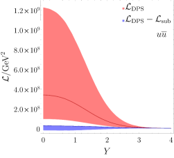
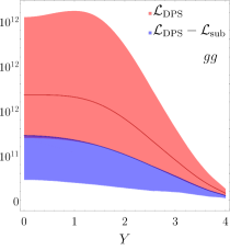
Refer to caption
Refer to caption
Figure 13: DPS luminosity DPSsubscriptDPS\mathcal{L}_{\text{DPS}} and the difference DPS1v1,ptsubscriptDPSsubscript1v1,pt\mathcal{L}_{\text{DPS}}-\mathcal{L}_{\text{1v1,pt}} between the DPS and subtraction luminosities, shown for the uu¯𝑢¯𝑢u\bar{u} (a) and gg𝑔𝑔gg (b) channels. Kinematic conditions are as in figure 9.2.2. In the case of DPS1v1,ptsubscriptDPSsubscript1v1,pt\mathcal{L}_{\text{DPS}}-\mathcal{L}_{\text{1v1,pt}}, the value for ν=80GeV𝜈80GeV\nu=80\operatorname{GeV} is always at the top of the scale variation band.

We plot DPSsubscriptDPS\mathcal{L}_{\text{DPS}} and DPS1v1,ptsubscriptDPSsubscript1v1,pt\mathcal{L}_{\text{DPS}}-\mathcal{L}_{\text{1v1,pt}} for the uu¯𝑢¯𝑢u\bar{u} and gg𝑔𝑔gg channels in figure 13. The lines are the values for ν=80GeV𝜈80GeV\nu=80\operatorname{GeV}, whilst the bands show the variation when ν𝜈\nu is varied by a factor of 222 up and down. Note that for DPS1v1,ptsubscriptDPSsubscript1v1,pt\mathcal{L}_{\text{DPS}}-\mathcal{L}_{\text{1v1,pt}}, the curve with ν=80GeV𝜈80GeV\nu=80\operatorname{GeV} is always at the very top of the scale variation band. We see that the ν𝜈\nu scale variation of DPS1v1,ptsubscriptDPSsubscript1v1,pt\mathcal{L}_{\text{DPS}}-\mathcal{L}_{\text{1v1,pt}} is indeed reduced compared to DPSsubscriptDPS\mathcal{L}_{\text{DPS}}, with the reduction being much stronger for uu¯𝑢¯𝑢u\bar{u} than for gg𝑔𝑔gg. The latter is consistent with our previous observation that evolution effects are weaker in the uu¯𝑢¯𝑢u\bar{u} channel at central rapidities: if evolution effects are weak, Fsplsubscript𝐹splF_{\text{spl}} and Fspl,fosubscript𝐹spl,foF_{\text{spl,fo}} have a similar y𝑦y dependence, so that (Fspl×FsplFspl,fo×Fspl,fo)subscript𝐹splsubscript𝐹splsubscript𝐹spl,fosubscript𝐹spl,fo(F_{\text{spl}}\times F_{\text{spl}}-F_{\text{spl,fo}}\times F_{\text{spl,fo}}) is flat in y𝑦y space and DPS1v1,ptsubscriptDPSsubscript1v1,pt\mathcal{L}_{\text{DPS}}-\mathcal{L}_{\text{1v1,pt}} varies weakly with ν𝜈\nu.

In section 6.2 we argued on generic grounds that the ν𝜈\nu variation of the 1v1 contribution to σDPSsubscript𝜎DPS\sigma_{\text{DPS}} should be of the same order as the subtraction term σ1v1,ptsubscript𝜎1v1,pt\sigma_{\text{1v1,pt}}. This is confirmed in figure 13, where the size of 1v1,ptsubscript1v1,pt\mathcal{L}_{\text{1v1,pt}} (evaluated at central ν𝜈\nu) can be read off from the distance between the central curve for DPSsubscriptDPS\mathcal{L}_{\text{DPS}} and the top of the band for DPS1v1,ptsubscriptDPSsubscript1v1,pt\mathcal{L}_{\text{DPS}}-\mathcal{L}_{\text{1v1,pt}}. This finding allows us to sharpen the argument we already made in the discussion of figure 9.2.2: not only does a large ν𝜈\nu variation of the 1v1 contribution to σDPSsubscript𝜎DPS\sigma_{\text{DPS}} indicate the need to include SPS and the associated subtraction term in the cross section, but the size of the ν𝜈\nu variation may even serve as a rough estimate for the size of these terms.

[Uncaptioned image]
Figure 14: Splitting DPDs Fsplsubscript𝐹splF_{\text{spl}} as a function of y𝑦y, with x1=x2=5.7×10³subscript𝑥1subscript𝑥25.7superscript103x_{1}=x_{2}=5.7\times 10^{-3} and μ=80GeV𝜇80GeV\mu=80\operatorname{GeV}. The parton combinations shown are uu¯𝑢¯𝑢u\bar{u} (a), gg𝑔𝑔gg (b) and ug𝑢𝑔ug (c). The vertical grey lines correspond to y=b0/(160GeV)𝑦subscript𝑏0160GeVy=b_{0}/(160\operatorname{GeV}), y=b0/(80GeV)𝑦subscript𝑏080GeVy=b_{0}/(80\operatorname{GeV}) and y=b0/(40GeV)𝑦subscript𝑏040GeVy=b_{0}/(40\operatorname{GeV}).

To better understand the behaviour we have seen in the 1v1 luminosities for the uu¯𝑢¯𝑢u\bar{u} and gg𝑔𝑔gg channels, we now take a closer look at how evolution affects the y𝑦y dependence of splitting DPDs. In figure 9.2.2 we plot Fspl(𝒚;μ)subscript𝐹spl𝒚𝜇F_{\text{spl}}(\boldsymbol{y};\mu) against y𝑦y, setting x1=x2=5.7×10³subscript𝑥1subscript𝑥25.7superscript103x_{1}=x_{2}=5.7\times 10^{-3} so that the uu¯𝑢¯𝑢u\bar{u} and gg𝑔𝑔gg DPDs are the ones used for the point Y=0𝑌0Y=0 in figures 9.2.2 and 13. We also plot the ug𝑢𝑔ug DPD, which mixes with uu¯𝑢¯𝑢u\bar{u} and gg𝑔𝑔gg under evolution. For comparison we show Fspl,fo(𝒚;μ)subscript𝐹spl,fo𝒚𝜇F_{\text{spl,fo}}(\boldsymbol{y};\mu), as well as the initial condition Fspl,ini(𝒚)=Fspl(𝒚;μy)subscript𝐹spl,ini𝒚subscript𝐹spl𝒚subscript𝜇𝑦F_{\text{spl,ini}}(\boldsymbol{y})=F_{\text{spl}}(\boldsymbol{y};\mu_{y}) given in (9.2.1), from which Fspl(𝒚;μ)subscript𝐹spl𝒚𝜇F_{\text{spl}}(\boldsymbol{y};\mu) is obtained by evolution. The distributions are plotted in the range b0/(160GeV)<y<b0/(40GeV)subscript𝑏0160GeV𝑦subscript𝑏040GeVb_{0}/(160\operatorname{GeV})<y<b_{0}/(40\operatorname{GeV}), i.e. in the range over which the lower integration limit in y𝑦y is varied when we vary ν𝜈\nu between 40GeV40GeV40\operatorname{GeV} to 160GeV160GeV160\operatorname{GeV}. In this region, the exponential damping factor in our DPD model is irrelevant, so that Fspl,inisubscript𝐹spl,iniF_{\text{spl,ini}} and Fspl,fosubscript𝐹spl,foF_{\text{spl,fo}} only differ by the scales taken in αssubscript𝛼𝑠\alpha_{s} and fa0(x1+x2)subscript𝑓subscript𝑎0subscript𝑥1subscript𝑥2f_{a_{0}}(x_{1}+x_{2}).

For the initial conditions Fspl,inisubscript𝐹spl,iniF_{\text{spl,ini}} we note that the uu¯𝑢¯𝑢u\bar{u} and ug𝑢𝑔ug distributions are of similar size; the former is initialised by a larger PDF (fgsubscript𝑓𝑔f_{g} instead of fusubscript𝑓𝑢f_{u}) but has a smaller splitting coefficient P(1/2)𝑃12P(1/2) as we noted before (9.1). By contrast, the gg𝑔𝑔gg distribution is much bigger; here both the initialising PDF and the splitting coefficient are large.

By construction, all three curves in each plot are equal at y=b0/(80GeV)𝑦subscript𝑏080GeVy=b_{0}/(80\operatorname{GeV}), when μy=μsubscript𝜇𝑦𝜇\mu_{y}=\mu. In all plots, Fspl,inisubscript𝐹spl,iniF_{\text{spl,ini}} has a more shallow y𝑦y behaviour than Fspl,fosubscript𝐹spl,foF_{\text{spl,fo}}. This difference is mainly driven by αssubscript𝛼𝑠\alpha_{s}, as the PDFs do not vary so much between μysubscript𝜇𝑦\mu_{y} and μ𝜇\mu at momentum fraction x1+x2=1.14×10²subscript𝑥1subscript𝑥21.14superscript102x_{1}+x_{2}=1.14\times 10^{-2}. One observes that the difference between Fsplsubscript𝐹splF_{\text{spl}} and Fspl,inisubscript𝐹spl,iniF_{\text{spl,ini}} is more significant for gg𝑔𝑔gg and ug𝑢𝑔ug than for uu¯𝑢¯𝑢u\bar{u}, i.e. that DPD evolution has a much stronger effect on the former two channels. This is to be expected at small x𝑥x, since the 1/v1𝑣1/v behaviour of the splitting kernels Pgg(v)subscript𝑃𝑔𝑔𝑣P_{gg}(v) and Pgq(v)subscript𝑃𝑔𝑞𝑣P_{gq}(v) at small v𝑣v favours the radiation of a gluon with much smaller momentum than its parent parton, whereas the kernels Pqq(v)subscript𝑃𝑞𝑞𝑣P_{qq}(v) and Pqg(v)subscript𝑃𝑞𝑔𝑣P_{qg}(v) giving a quark stay finite for v0𝑣0v\to 0.

An interesting point to note is that, whilst for gg𝑔𝑔gg and ug𝑢𝑔ug the curves for Fsplsubscript𝐹splF_{\text{spl}} are more shallow than for Fspl,inisubscript𝐹spl,iniF_{\text{spl,ini}}, in the case of uu¯𝑢¯𝑢u\bar{u} the Fsplsubscript𝐹splF_{\text{spl}} curve is actually steeper. The latter is surprising since — based on the experience with single PDFs at small x𝑥x — one may expect that forward evolution for y>b0/(80GeV)𝑦subscript𝑏080GeVy>b_{0}/(80\operatorname{GeV}) would always increase a DPD, and backward evolution for y<b0/(80GeV)𝑦subscript𝑏080GeVy<b_{0}/(80\operatorname{GeV}) would always decrease it. This indeed happens in the gg𝑔𝑔gg and ug𝑢𝑔ug channels, whilst forward evolution results in a decrease of the uu¯𝑢¯𝑢u\bar{u} DPD. The reason for this is that Fug,splsubscript𝐹𝑢𝑔splF_{ug,\mskip 1.5mu\text{spl}} and Fgu¯,splsubscript𝐹𝑔¯𝑢splF_{g\bar{u},\mskip 1.5mu\text{spl}}, which directly feed into Fuu¯,splsubscript𝐹𝑢¯𝑢splF_{u\bar{u},\mskip 1.5mu\text{spl}} during evolution, are comparatively small. In the case of PDFs, fgsubscript𝑓𝑔f_{g} is much larger than fusubscript𝑓𝑢f_{u} and hence can drive its small-x𝑥x evolution although the splitting function Pqgsubscript𝑃𝑞𝑔P_{qg} does not favour the radiation of low-momentum quarks. The evolution of the gg𝑔𝑔gg and ug𝑢𝑔ug DPDs is driven by the large distribution Fgg,splsubscript𝐹𝑔𝑔splF_{gg,\mskip 1.5mu\text{spl}} and enhanced by the Pggsubscript𝑃𝑔𝑔P_{gg} splitting function.

Note that in all three channels, Fsplsubscript𝐹splF_{\text{spl}} has a smaller slope in y𝑦y than Fspl,fosubscript𝐹spl,foF_{\text{spl,fo}}. This implies that the y𝑦y integrand for the computation of DPS1v1,ptsubscriptDPSsubscript1v1,pt\mathcal{L}_{\text{DPS}}-\mathcal{L}_{\text{1v1,pt}} is positive for y>b0/(80GeV)𝑦subscript𝑏080GeVy>b_{0}/(80\operatorname{GeV}) and negative for y<b0/(80GeV)𝑦subscript𝑏080GeVy<b_{0}/(80\operatorname{GeV}). Therefore, the DPS1v1,ptsubscriptDPSsubscript1v1,pt\mathcal{L}_{\text{DPS}}-\mathcal{L}_{\text{1v1,pt}} curves for ν=40GeV𝜈40GeV\nu=40\operatorname{GeV} and ν=160GeV𝜈160GeV\nu=160\operatorname{GeV} lie below that for ν=80GeV𝜈80GeV\nu=80\operatorname{GeV}. The curve for the central ν𝜈\nu value thus lies at the top of the ν𝜈\nu variation band, as we already observed in figure 13.

For uu¯𝑢¯𝑢u\bar{u}, the evolution from μysubscript𝜇𝑦\mu_{y} to μ𝜇\mu turns out to have much the same quantitative effect as adjusting the scale in the fixed order expression from μysubscript𝜇𝑦\mu_{y} to μ𝜇\mu, such that Fsplsubscript𝐹splF_{\text{spl}} and Fspl,fosubscript𝐹spl,foF_{\text{spl,fo}} end up extremely close together. This explains why at central rapidities the ν𝜈\nu variation of the 1v1 uu¯𝑢¯𝑢u\bar{u} contribution in figure 9.2.2a coincides almost exactly with the naive prediction from (9.1), which assumes that Fsplsubscript𝐹splF_{\text{spl}} depends on y𝑦y like y2superscript𝑦2y^{-2} (as does Fspl,fosubscript𝐹spl,foF_{\text{spl,fo}}). Furthermore, if Fsplsubscript𝐹splF_{\text{spl}} and Fspl,fosubscript𝐹spl,foF_{\text{spl,fo}} are very close to each other, then DPS1v1,ptsubscriptDPSsubscript1v1,pt\mathcal{L}_{\text{DPS}}-\mathcal{L}_{\text{1v1,pt}} is much smaller than DPSsubscriptDPS\mathcal{L}_{\text{DPS}}, which we indeed see in figure 13a.

In the gg𝑔𝑔gg channel, the modification of the y𝑦y slope by evolution is significant. In the range of figure 9.2.2, the y𝑦y dependence is changed from y2superscript𝑦2y^{-2} at the starting scale to approximately y1.4superscript𝑦1.4y^{-1.4}. One may expect this flattening effect to become even stronger as the x𝑥x values in the DPDs decrease. The dependence of DPSsubscriptDPS\mathcal{L}_{\text{DPS}} on the scale ν𝜈\nu should then decrease. This was already anticipated in Ryskin:2011kk ; Ryskin:2012qx , where studies in the double leading logarithm approximation were performed.

[Uncaptioned image]
Figure 15: DPS luminosities in the gg𝑔𝑔gg channel with all x𝑥x values in the DPDs set equal. The collider energy s𝑠\sqrt{s} is fixed to 14TeV14TeV14\operatorname{TeV} (a) or to 100TeV100TeV100\operatorname{TeV} (b). The scales of the DPDs, set to μ=xs𝜇𝑥𝑠\mu=x\sqrt{s}, are given at the top of the plot.

Here we investigate this effect using our full LO DGLAP set-up. We consider the gg𝑔𝑔gg channel with all x𝑥x values set equal and study the DPS luminosity as a function of the common x𝑥x value. We fix the collider energy s𝑠\sqrt{s}, so that the scale μ=Q1=Q2=xs𝜇subscript𝑄1subscript𝑄2𝑥𝑠\mu=Q_{1}=Q_{2}=x\sqrt{s} also varies with x𝑥x. We make one plot with s=14TeV𝑠14TeV\sqrt{s}=14\operatorname{TeV} and 5×10⁴<x<0.25superscript104𝑥0.25\times 10^{-4}<x<0.2 (corresponding to 7GeV<μ<2800GeV7GeV𝜇2800GeV7\operatorname{GeV}<\mu<2800\operatorname{GeV}) and another one with higher collider energy s=100TeV𝑠100TeV\sqrt{s}=100\operatorname{TeV} and 104<x<0.02superscript104𝑥0.0210^{-4}<x<0.02 (corresponding to 10GeV<μ<2000GeV10GeV𝜇2000GeV10\operatorname{GeV}<\mu<2000\operatorname{GeV}). In our numerical code this requires a new DPD grid with larger μ𝜇\mu and μysubscript𝜇𝑦\mu_{y} ranges, which was generated using 60 points in the μ𝜇\mu and μysubscript𝜇𝑦\mu_{y} directions (as in the original grid). The resulting 1v1 luminosity is shown in figure 9.2.2, with bands for the ν𝜈\nu variation and its naive version as in figure 9.2.2. For comparison we also show the 2v1 and 2v2 luminosities.

We see that the ν𝜈\nu variation does indeed become progressively smaller compared to the central value as x𝑥x (and μ𝜇\mu) decreases. At the lowest x𝑥x values it is much smaller than the naive expectation. At larger x𝑥x, where evolution has a smaller effect on the DPDs, the ν𝜈\nu variation becomes larger: for s=14TeV𝑠14TeV\sqrt{s}=14\operatorname{TeV} the actual and naive ν𝜈\nu bands essentially coincide towards the right of the plot, where values of the order of x0.1similar-to𝑥0.1x\sim 0.1 are reached. Towards the left of each plot, where x𝑥x and μ𝜇\mu become small, the 2v2 and 2v1 contributions begin to dominate over 1v1. For given μ𝜇\mu, this effect is more pronounced for s=100TeV𝑠100TeV\sqrt{s}=100\operatorname{TeV} than for s=14TeV𝑠14TeV\sqrt{s}=14\operatorname{TeV}, since the x𝑥x values in the former case are smaller. We note that in the uu¯𝑢¯𝑢u\bar{u} channel (not shown here) the actual and naive ν𝜈\nu bands remain very similar throughout the kinematics of figure 9.2.2.
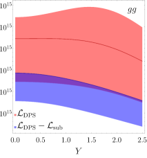
Refer to caption
Figure 16: As in figure 13b, but for different kinematics, with μ=10GeV𝜇10GeV\mu=10\operatorname{GeV} and all x𝑥x set equal to 7.1×1047.1superscript1047.1\times 10^{-4}, corresponding to Q1=Q2=10GeVsubscript𝑄1subscript𝑄210GeVQ_{1}=Q_{2}=10\operatorname{GeV} at s=14TeV𝑠14TeV\sqrt{s}=14\operatorname{TeV}. Notice the suppressed zero on the \mathcal{L} axis.

For the small x𝑥x values where the ν𝜈\nu variation is small in figure 9.2.2, the gg𝑔𝑔gg splitting DPD is significantly shallower in y𝑦y than the fixed-order y2superscript𝑦2y^{-2} form. For s=14TeV𝑠14TeV\sqrt{s}=14\operatorname{TeV} we find that around x=2×10³𝑥2superscript103x=2\times 10^{-3} it reaches y1superscript𝑦1y^{-1}, implying a logarithmic dependence on ν𝜈\nu in DPSsubscript𝐷𝑃𝑆\mathcal{L}_{DPS}, whilst a behaviour like y0.5superscript𝑦0.5y^{-0.5} is reached around 5×1045superscript1045\times 10^{-4}. For s=100TeV𝑠100TeV\sqrt{s}=100\operatorname{TeV} the y𝑦y behaviour is like y1superscript𝑦1y^{-1} around x=4×10⁴𝑥4superscript104x=4\times 10^{-4} and like y0.5superscript𝑦0.5y^{-0.5} around x=104𝑥superscript104x=10^{-4}. In such a regime, the bulk of the contribution to the 1v1 part of DPSsubscriptDPS\mathcal{L}_{\text{DPS}} comes from large distances y1/νmuch-greater-than𝑦1𝜈y\gg 1/\nu, where the DPS approximations used to derive σDPSsubscript𝜎DPS\sigma_{\text{DPS}} are valid. Also, the 1v1 part of σDPSsubscript𝜎DPS\sigma_{\text{DPS}} becomes clearly larger than its ν𝜈\nu variation. As we argued earlier, the ν𝜈\nu variation should be of the same size as the subtraction term. This is confirmed in figure 16, which is analogous to figure 13b but for the kinematics of the point with μ=10GeV𝜇10GeV\mu=10\operatorname{GeV} in figure 9.2.2a. Using our argument that σ1v1,ptsubscript𝜎1v1,pt\sigma_{\text{1v1,pt}} is of the same magnitude as the order of σSPSsubscript𝜎SPS\sigma_{\text{SPS}} that contains the lowest-order DPS-type loop, one may in this situation justifiably make predictions that include the DPS piece but omit the order of SPS just specified, as well as the associated subtraction term. This is encouraging, for instance in the context of four-jet production, where the computation of the relevant SPS order (namely NNLO) is well beyond the current state of the art. Note that lower orders in SPS should be computed and included, if possible.

Notice that when the y𝑦y behaviour of Fsplsubscript𝐹splF_{\text{spl}} becomes flatter than y1superscript𝑦1y^{-1}, the dominant y𝑦y region in the 1v1 part of DPSsubscriptDPS\mathcal{L}_{\text{DPS}} shifts to values y1/Λsimilar-to𝑦1Λy\sim 1/\Lambda, where one cannot compute the splitting DPD in perturbation theory and must rely on a model. Likewise, the 2v1 part of DPSsubscriptDPS\mathcal{L}_{\text{DPS}} becomes increasingly sensitive to the region y1/Λsimilar-to𝑦1Λy\sim 1/\Lambda as soon as Fsplsubscript𝐹splF_{\text{spl}} becomes flatter than the fixed-order form y2superscript𝑦2y^{-2}.

Refer to caption
Refer to caption
Figure 17: Double parton scattering luminosities a1a2b1b2(Y)subscriptsubscript𝑎1subscript𝑎2subscript𝑏1subscript𝑏2𝑌\mathcal{L}_{a_{1}a_{2}b_{1}b_{2}}(Y) for the production of two systems with Q1=Q2=80GeVsubscript𝑄1subscript𝑄280GeVQ_{1}=Q_{2}=80\operatorname{GeV} at s=14TeV𝑠14TeV\sqrt{s}=14\operatorname{TeV}, one with rapidity Y𝑌Y and the other with rapidity Y𝑌-Y. The parton combinations a1a2b1b2subscript𝑎1subscript𝑎2subscript𝑏1subscript𝑏2a_{1}a_{2}\mskip 1.5mub_{1}b_{2} are uu¯u¯u+u¯uuu¯𝑢¯𝑢¯𝑢𝑢¯𝑢𝑢𝑢¯𝑢u\bar{u}\bar{u}u+\bar{u}uu\bar{u} (a) and gggg𝑔𝑔𝑔𝑔gggg (b).

Another kinematic regime where the 1v1 contribution to DPSsubscriptDPS\mathcal{L}_{\text{DPS}} becomes large compared with its ν𝜈\nu variation and compared with 1v1,ptsubscript1v1,pt\mathcal{L}_{\text{1v1,pt}} is when the two hard systems have a large separation in rapidity. This reduction of the ν𝜈\nu variation can be seen as Y𝑌Y approaches 444 in figure 9.2.2, but only in the uu¯𝑢¯𝑢u\bar{u} and not in the gg𝑔𝑔gg channel. In both channels, the effect becomes more pronounced once the rapidity separation of the hard systems is increased beyond 444. To illustrate this, we make plots similar to figure 9.2.2 but now with one hard system at rapidity Y𝑌Y and the other at rapidity Y𝑌-Y (rather than one at Y𝑌Y and the other at 00), such that a given value of Y𝑌Y corresponds to a rapidity separation of 2Y2𝑌2Y. The results are shown in figure 17, where we see that the ν𝜈\nu variation in the 1v1 contribution is strongly reduced towards the right hand side of the plots, becoming hardly visible in the uu¯𝑢¯𝑢u\bar{u} channel. Also notable is the fact that for large Y𝑌Y, the 2v2 contribution in this channel exceeds 1v1, which strongly decreases between Y=0𝑌0Y=0 and 222.

This reduction in ν𝜈\nu dependence can be explained by the fact that at large Y𝑌Y we probe splitting DPDs with one large x𝑥x and one small x𝑥x parton. From the point of view of small x𝑥x logarithms, it is preferable to generate such a configuration by having the 12121\to 2 splitting at large x𝑥x, generating directly the large x𝑥x parton plus a gluon with smaller x𝑥x, the latter of which splits in a number of stages into smaller x𝑥x gluons, eventually yielding the small x𝑥x parton. This increasingly happens with increasing y𝑦y, since the “evolution distance” between the initial and final scales, μysubscript𝜇𝑦\mu_{y} and μ𝜇\mu, is increased. Thus, evolution again flattens the DPD compared to the naive y2superscript𝑦2y^{-2} expectation and reduces the ν𝜈\nu dependence of the DPS luminosities.

The effect is particularly drastic in the uu¯𝑢¯𝑢u\bar{u} channel, because the lowest-order splitting guu¯𝑔𝑢¯𝑢g\to u\bar{u} is inefficient at generating a pair with very different x𝑥x values (as Pgqq¯(v)subscript𝑃𝑔𝑞¯𝑞𝑣P_{g\to q\bar{q}}(v) goes to a constant at small v𝑣v). Therefore, the repeated splitting mechanism described in the previous paragraph is strongly preferred, even though its last step is penalised by the lack of small-v𝑣v enhancement in Pgq(v)subscript𝑃𝑔𝑞𝑣P_{gq}(v). In figure 18 we plot the uu¯𝑢¯𝑢u\bar{u} DPD in the x1x2much-less-thansubscript𝑥1subscript𝑥2x_{1}\ll x_{2} configuration relevant for Y=4𝑌4Y=4 in figure 17a. It has a similar y𝑦y dependence as the ud¯𝑢¯𝑑u\bar{d} DPD in equal kinematics, with the curve for ud¯𝑢¯𝑑u\bar{d} crossing zero exactly at y=b0/μ𝑦subscript𝑏0𝜇y=b_{0}/\mu (by construction), and the curve for uu¯𝑢¯𝑢u\bar{u} crossing zero rather close to this point. In the former case, the lowest-order 12121\to 2 splitting process is forbidden, whereas in the latter it is numerically almost irrelevant. The situation for x1x2much-greater-thansubscript𝑥1subscript𝑥2x_{1}\gg x_{2} is the same.

Refer to caption
Figure 18: As figure 9.2.2a but for asymmetric kinematics x1=104subscript𝑥1superscript104x_{1}=10^{-4}, x2=0.31subscript𝑥20.31x_{2}=0.31 at μ=80GeV𝜇80GeV\mu=80\operatorname{GeV}, which is needed for the point Y=4𝑌4Y=4 in figure 17a.

To end this section, we study polarised distributions and luminosities. We limit ourselves to the splitting part Fsplsubscript𝐹splF_{\text{spl}} of the DPD and to the 1v1 contribution to DPSsubscriptDPS\mathcal{L}_{\text{DPS}}. In fact, we have little guidance for modelling the intrinsic part Fintsubscript𝐹intF_{\text{int}}, where a product ansatz as in (9.2.1) makes no sense. We note that in Diehl:2014vaa , different ansätze were made for polarised DPDs, and the effects of evolution on these distributions were investigated. It was found that, in many cases, evolution to higher scales leads to a suppression of the polarised DPD with respect to its unpolarised counterpart.

We initialise the polarised Fsplsubscript𝐹splF_{\text{spl}} at μysubscript𝜇𝑦\mu_{y} using the expression in (9.2.1) with the unpolarised 12121\to 2 splitting functions replaced by their polarised counterparts (given in Appendix B of Diehl:2014vaa ). These distributions are then evolved to the scale μ𝜇\mu using the appropriate polarised double DGLAP equations (the required polarised splitting functions are collected in Appendix A of Diehl:2013mla ). The settings we used for the evolution code are the same as specified in section 9.2.1.
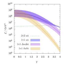
Refer to caption
Refer to caption
Figure 19: As in figure 9.2.2, but with two polarised 1v1 luminosity bands included in each case (and the unpolarised 2v1 band omitted).

We consider the same scenario as in figure 9.2.2, i.e. the production of two systems with Q1=Q2=80GeVsubscript𝑄1subscript𝑄280GeVQ_{1}=Q_{2}=80\operatorname{GeV} at s=14TeV𝑠14TeV\sqrt{s}=14\operatorname{TeV}, one with rapidity 00 and the other with rapidity Y𝑌Y, and now include polarised 1v1 contributions. In figure 19a, we reproduce figure 9.2.2a but include 1v1 luminosities for the polarised parton combinations a1a2b1b2=ΔuΔu¯Δu¯Δu+Δu¯ΔuΔuΔu¯subscript𝑎1subscript𝑎2subscript𝑏1subscript𝑏2Δ𝑢Δ¯𝑢Δ¯𝑢Δ𝑢Δ¯𝑢Δ𝑢Δ𝑢Δ¯𝑢a_{1}a_{2}\mskip 1.5mub_{1}b_{2}=\Delta u\Delta\bar{u}\Delta\bar{u}\Delta u+\Delta\bar{u}\Delta u\Delta u\Delta\bar{u} and δuδu¯δu¯δu+δu¯δuδuδu¯𝛿𝑢𝛿¯𝑢𝛿¯𝑢𝛿𝑢𝛿¯𝑢𝛿𝑢𝛿𝑢𝛿¯𝑢\delta u\mskip 1.5mu\delta\bar{u}\mskip 1.5mu\delta\bar{u}\mskip 1.5mu\delta u+\delta\bar{u}\mskip 1.5mu\delta u\mskip 1.5mu\delta u\mskip 1.5mu\delta\bar{u}. For brevity we refer to these combinations as ΔuΔu¯Δ𝑢Δ¯𝑢\Delta u\Delta\bar{u} and δuδu¯𝛿𝑢𝛿¯𝑢\delta u\mskip 1.5mu\delta\bar{u} in the following, recalling that ΔqΔ𝑞\Delta q and δq𝛿𝑞\delta q indicate longitudinal and transverse quark polarisation, respectively. These polarised luminosities appear in the DPS cross section for double Z𝑍Z production, see section 3.1 of Kasemets:2012pr (combinations like uu¯Δu¯Δu𝑢¯𝑢Δ¯𝑢Δ𝑢u\bar{u}\mskip 1.5mu\Delta\bar{u}\Delta u also appear but are not shown here). To avoid cluttering the plots, we omit the unpolarised 2v1 luminosity, reminding the reader that it is of the same magnitude as 2v2. In figure 19b we repeat the exercise for the pure gluon channel, including the 1v1 luminosities for the polarised combinations a1a2b1b2=ΔgΔgΔgΔgsubscript𝑎1subscript𝑎2subscript𝑏1subscript𝑏2Δ𝑔Δ𝑔Δ𝑔Δ𝑔a_{1}a_{2}\mskip 1.5mub_{1}b_{2}=\Delta g\Delta g\Delta g\Delta g and δgδgδgδg𝛿𝑔𝛿𝑔𝛿𝑔𝛿𝑔\delta g\mskip 1.5mu\delta g\mskip 1.5mu\delta g\mskip 1.5mu\delta g, referred to as ΔgΔgΔ𝑔Δ𝑔\Delta g\Delta g and δgδg𝛿𝑔𝛿𝑔\delta g\mskip 1.5mu\delta g, where ΔgΔ𝑔\Delta g and δg𝛿𝑔\delta g respectively denote longitudinal and linear gluon polarisation.

We see that the 1v1 luminosities for ΔuΔu¯Δ𝑢Δ¯𝑢\Delta u\Delta\bar{u} and δuδu¯𝛿𝑢𝛿¯𝑢\delta u\mskip 1.5mu\delta\bar{u} essentially coincide with the one for uu¯𝑢¯𝑢u\bar{u} at central rapidities, with ν𝜈\nu variation bands of very similar size. These observations can be explained by the fact that at Y=0𝑌0Y=0 we initialise all three DPDs using the same expression up to a minus sign, with Pgqq¯=|PgΔqΔq¯|=|Pgδqδq¯|subscript𝑃𝑔𝑞¯𝑞subscript𝑃𝑔Δ𝑞Δ¯𝑞subscript𝑃𝑔𝛿𝑞𝛿¯𝑞P_{g\to q\bar{q}}=|P_{g\to\Delta q\Delta\bar{q}}|=|P_{g\to\delta q\mskip 1.5mu\delta\bar{q}}| at v=1/2𝑣12v=1/2, and that evolution has a rather weak effect on all three DPDs for central rapidities. This close agreement extends out to higher values of Y𝑌Y for the uu¯𝑢¯𝑢u\bar{u} and ΔuΔu¯Δ𝑢Δ¯𝑢\Delta u\Delta\bar{u} curves, owing to the fact that Pgqq¯=|PgΔqΔq¯|subscript𝑃𝑔𝑞¯𝑞subscript𝑃𝑔Δ𝑞Δ¯𝑞P_{g\to q\bar{q}}=|P_{g\to\Delta q\Delta\bar{q}}| for general v𝑣v. By contrast, the δuδu¯𝛿𝑢𝛿¯𝑢\delta u\mskip 1.5mu\delta\bar{u} curve clearly falls below the other two for larger Y𝑌Y, because Pgqq¯>|Pgδqδq¯|subscript𝑃𝑔𝑞¯𝑞subscript𝑃𝑔𝛿𝑞𝛿¯𝑞P_{g\to q\bar{q}}>|P_{g\to\delta q\mskip 1.5mu\delta\bar{q}}| for v1/2𝑣12v\neq 1/2.

In figure 19b, the δgδg𝛿𝑔𝛿𝑔\delta g\mskip 1.5mu\delta g luminosity lies well below the one for ΔgΔgΔ𝑔Δ𝑔\Delta g\Delta g, which in turn lies somewhat below the one for gg𝑔𝑔gg. This is mostly driven by the differences in initialisation expressions for the DPDs: at v=1/2𝑣12v=1/2 (relevant at Y=0𝑌0Y=0) the relevant splitting function satisfy for instance Pggg:PgΔgΔg:Pgδgδg=9:7:1:subscript𝑃𝑔𝑔𝑔subscript𝑃𝑔Δ𝑔Δ𝑔:subscript𝑃𝑔𝛿𝑔𝛿𝑔9:7:1P_{g\to gg}:P_{g\to\Delta g\Delta g}:P_{g\to\delta g\mskip 1.5mu\delta g}=9:7:1. Ignoring evolution effects, one would then expect the gg𝑔𝑔gg luminosity at Y=0𝑌0Y=0 to be roughly 1.51.51.5 times bigger than the one for ΔgΔgΔ𝑔Δ𝑔\Delta g\Delta g, which in turn should be roughly 505050 times bigger than the one for δgδg𝛿𝑔𝛿𝑔\delta g\mskip 1.5mu\delta g. This expectation is quite close to the actual luminosity ratios, which are 4similar-toabsent4\sim 4 and 60similar-toabsent60\sim 60, respectively. The remaining difference is due to evolution effects, which increase gg𝑔𝑔gg rather considerably, increase ΔgΔgΔ𝑔Δ𝑔\Delta g\Delta g to a lesser extent, and hardly change δgδg𝛿𝑔𝛿𝑔\delta g\delta g.

Overall, we see that the polarised 1v1 luminosities can be of the same order of magnitude as the unpolarised ones, so that one must in general take into account all possible polarisation combinations in the DPS contribution, together with the SPS term and subtraction (where the subtraction will also contain both unpolarised and polarised contributions).

9.3 Production of two scalars

In this section, we study an explicit example to test our general argument that σ1v1,ptsubscript𝜎1v1,pt\sigma_{\text{1v1,pt}} is of similar size as the corresponding perturbative order of the SPS cross section. The process we investigate is an artificial one, chosen for ease of computation. We consider the hypothetical production of two identical massive scalar bosons ϕitalic-ϕ\phi, which couple to quarks with a Yukawa term cϕq¯q𝑐italic-ϕ¯𝑞𝑞c\mskip 1.5mu\phi\mskip 1.5mu\bar{q}q, where c𝑐c is a constant. For simplicity we take only one light quark flavour; including further light flavours just multiplies all following results (SPS and subtraction) by nfsubscript𝑛𝑓n_{f}. We will not compare the subtraction term to the full SPS contribution, but rather to the gg𝑔𝑔gg initiated part of σSPSsubscript𝜎SPS\sigma_{\text{SPS}}, which is the piece that contains the lowest order DPS-type ggϕϕ𝑔𝑔italic-ϕitalic-ϕgg\to\phi\phi box diagram. This piece is gauge invariant and can hence be meaningfully considered by itself.

In keeping with the notation of the paper, let us denote the mass of each produced boson ϕitalic-ϕ\phi by Q𝑄Q. Let Y𝑌Y be the rapidity of the diboson system in the pp𝑝𝑝pp centre-of-mass frame, s^^𝑠\hat{s} its squared invariant mass, and β=14Q2/s^𝛽14superscript𝑄2^𝑠\beta=\sqrt{1-4Q^{2}/\hat{s}} the velocity of one boson in the diboson centre-of-mass frame. The ggϕϕ𝑔𝑔italic-ϕitalic-ϕgg\to\phi\phi part of the SPS cross section can be written as

dσSPSdYdβ𝑑subscript𝜎SPS𝑑𝑌𝑑𝛽\displaystyle\frac{d\sigma_{\text{SPS}}}{dYd\beta} =xx¯g(x)g(x¯)2β1β2σ^ggϕϕabsent𝑥¯𝑥𝑔𝑥𝑔¯𝑥2𝛽1superscript𝛽2subscript^𝜎𝑔𝑔italic-ϕitalic-ϕ\displaystyle=x\bar{x}\,g(x)\,g(\bar{x})\,\frac{2\beta}{1-\beta^{2}}\,\hat{\sigma}_{gg\to\phi\phi}
=xx¯g(x)g(x¯)1128π1β2Q40qmax2dq21q2/qmax2|𝒜ggϕϕ|2,absent𝑥¯𝑥𝑔𝑥𝑔¯𝑥1128𝜋1superscript𝛽2superscript𝑄4superscriptsubscript0subscriptsuperscript𝑞2max𝑑superscript𝑞21superscript𝑞2subscriptsuperscript𝑞2maxsuperscriptsubscript𝒜𝑔𝑔italic-ϕitalic-ϕ2\displaystyle=x\bar{x}\,g(x)\,g(\bar{x})\,\frac{1}{128\mskip 1.5mu\pi}\,\frac{1-\beta^{2}}{Q^{4}}\,\int_{0}^{q^{2}_{\text{max}}}\!\frac{dq^{2}}{\sqrt{1-q^{2}/q^{2}_{\text{max}}}}\,\bigl{|}\mathcal{A}_{gg\to\phi\phi}\bigr{|}^{2}\,, (157)

where qmax=βQ/1β2subscript𝑞max𝛽𝑄1superscript𝛽2q_{\text{max}}=\beta Q\big{/}\sqrt{1-\beta^{2}} and the ggϕϕ𝑔𝑔italic-ϕitalic-ϕgg\to\phi\phi matrix element squared, |𝒜ggϕϕ|2superscriptsubscript𝒜𝑔𝑔italic-ϕitalic-ϕ2|\mathcal{A}_{gg\to\phi\phi}|^{2}, is averaged over the spin and colour of the incoming gluons. The momentum fractions x𝑥x and x¯¯𝑥\bar{x} in the gluon distributions are obtained from the constraints s^=xx¯s^𝑠𝑥¯𝑥𝑠\hat{s}=x\bar{x}s and Y=12log(x/x¯)𝑌12𝑥¯𝑥Y={\tfrac{1}{2}}\log(x/\bar{x}).

The matrix element squared for ggϕϕ𝑔𝑔italic-ϕitalic-ϕgg\to\phi\phi can be obtained from the ggHH𝑔𝑔𝐻𝐻gg\to HH matrix element squared given in Glover:1987nx by making the replacement

παWmq2MW2c2.𝜋subscript𝛼𝑊superscriptsubscript𝑚𝑞2superscriptsubscript𝑀𝑊2superscript𝑐2\displaystyle\frac{\pi\alpha_{\scriptscriptstyle W}m_{q}^{2}}{M_{\scriptscriptstyle W}^{2}}\to c^{2}\,. (158)

In particular, |𝒜ggϕϕ|2superscriptsubscript𝒜𝑔𝑔italic-ϕitalic-ϕ2|\mathcal{A}_{gg\to\phi\phi}|^{2} in (9.3) is related to the terms “gauge1” and “gauge2” in Glover:1987nx according to

|𝒜ggϕϕ|2superscriptsubscript𝒜𝑔𝑔italic-ϕitalic-ϕ2\displaystyle\bigl{|}\mathcal{A}_{gg\to\phi\phi}\bigr{|}^{2} =c4αs2210π2mq4(|gauge1|2+|gauge2|2).absentsuperscript𝑐4superscriptsubscript𝛼𝑠2superscript210superscript𝜋2superscriptsubscript𝑚𝑞4superscriptgauge12superscriptgauge22\displaystyle=\dfrac{c^{4}\alpha_{s}^{2}}{2^{10}\pi^{2}m_{q}^{4}}\left(\left|\text{gauge1}\right|^{2}+\left|\text{gauge2}\right|^{2}\right)\,. (159)

The right hand side of (159) is given in Glover:1987nx for general quark mass mqsubscript𝑚𝑞m_{q}. We evaluate this expression numerically for very small mqsubscript𝑚𝑞m_{q}, using analytic mq0subscript𝑚𝑞0m_{q}\to 0 approximations where this is necessary to avoid numerical instabilities.

Now we turn to the subtraction term. The two elementary qq¯ϕ𝑞¯𝑞italic-ϕq\bar{q}\to\phi cross sections in this term contain the kinematic constraint 2πδ(xix¯isQ2)2𝜋𝛿subscript𝑥𝑖subscript¯𝑥𝑖𝑠superscript𝑄22\pi\delta(x_{i}\bar{x}_{i}\mskip 1.5mus-Q^{2}), which fixes the momentum fractions xisubscript𝑥𝑖x_{i} and x¯isubscript¯𝑥𝑖\bar{x}_{i} entering the two hard subprocesses at given x,x¯𝑥¯𝑥x,\bar{x} and β𝛽\beta up to a two-fold ambiguity. The DPS subtraction term is given by

dσ1v1,ptdYdβ𝑑subscript𝜎1v1,pt𝑑𝑌𝑑𝛽\displaystyle\frac{d\sigma_{\text{1v1,pt}}}{dYd\beta} =π2161β2Q8x2x¯2a1a2b1b2|𝒜a1b1ϕ|2|𝒜a2b2ϕ|2d2𝒚Φ2(yν)R=1,8absentsuperscript𝜋2161superscript𝛽2superscript𝑄8superscript𝑥2superscript¯𝑥2subscriptsubscript𝑎1subscript𝑎2subscript𝑏1subscript𝑏2superscriptsubscript𝒜subscript𝑎1subscript𝑏1italic-ϕ2superscriptsubscript𝒜subscript𝑎2subscript𝑏2italic-ϕ2superscript𝑑2𝒚superscriptΦ2𝑦𝜈subscript𝑅18\displaystyle=\frac{\pi^{2}}{16}\,\frac{1-\beta^{2}}{Q^{8}}\,x^{2}\bar{x}^{2}\sum_{a_{1}a_{2}b_{1}b_{2}}\bigl{|}\mathcal{A}_{a_{1}b_{1}\to\phi}\bigr{|}^{2}\,\bigl{|}\mathcal{A}_{a_{2}b_{2}\to\phi}\bigr{|}^{2}\int d^{2}\boldsymbol{y}\;\Phi^{2}(y\nu)\sum_{R=1,8}
×[Fa1a2,spl,ptR(12x(1+β),12x(1β),𝒚)Fb1b2,spl,ptR(12x¯(1β),12x¯(1+β),𝒚)\displaystyle\quad\times\biggl{[}{}^{R\!}F_{a_{1}a_{2},\mskip 1.5mu\text{spl,pt}}\Bigl{(}{\tfrac{1}{2}}x(1+\beta),{\tfrac{1}{2}}x(1-\beta),\boldsymbol{y}\Bigr{)}\,{}^{R\!}F_{b_{1}b_{2},\mskip 1.5mu\text{spl,pt}}\Bigl{(}{\tfrac{1}{2}}\bar{x}\mskip 1.5mu(1-\beta),{\tfrac{1}{2}}\bar{x}\mskip 1.5mu(1+\beta),\boldsymbol{y}\Bigr{)}
+{ββ}]+{FI},\displaystyle\qquad+\{\beta\to-\beta\}\biggr{]}+\{F\to I\}\,, (160)

where we sum over all possible colour, spin, and quark number interference/correlation possibilities. The index R𝑅R on F𝐹F denotes the colour channel (R=1𝑅1R=1 for colour singlet, R=8𝑅8R=8 for colour octet), and in the sum over a1a2b1b2subscript𝑎1subscript𝑎2subscript𝑏1subscript𝑏2a_{1}a_{2}\mskip 1.5mub_{1}b_{2} we sum over both unpolarised (e.g. qq¯q¯q𝑞¯𝑞¯𝑞𝑞q\bar{q}\bar{q}q) and polarised (e.g. ΔqΔq¯Δq¯ΔqΔ𝑞Δ¯𝑞Δ¯𝑞Δ𝑞\Delta q\Delta\bar{q}\Delta\bar{q}\Delta q) combinations. By {FI}𝐹𝐼\{F\to I\} we denote the same expression, but with the quark number diagonal distributions replaced by the quark number interference ones (see section 2 of Diehl:2011yj ).

The splitting kernels for the relevant spin combinations are Diehl:2011yj

Pgqq¯1(v)=PgΔqΔq¯1(v)superscriptsubscript𝑃𝑔𝑞¯𝑞1𝑣superscriptsubscript𝑃𝑔Δ𝑞Δ¯𝑞1𝑣\displaystyle{}^{1\!}P_{g\to q\bar{q}\,}(v)=-\,{}^{1\!}P_{g\to\Delta q\Delta\bar{q}\,}(v) =12[v2+(1v)2],absent12delimited-[]superscript𝑣2superscript1𝑣2\displaystyle=\frac{1}{2}\mskip 1.5mu\bigl{[}v^{2}+(1-v)^{2}\mskip 1.5mu\bigr{]}\,, Pgδqδq¯1(v)superscriptsubscript𝑃𝑔𝛿𝑞𝛿¯𝑞1𝑣\displaystyle{}^{1\!}P_{g\to\delta q\delta\bar{q}\,}(v) =δjjv(1v)absentsuperscript𝛿𝑗superscript𝑗𝑣1𝑣\displaystyle={}-\delta^{jj^{\prime}}v(1-v) (161)

and P8=P1/Nc21superscript𝑃8superscript𝑃1superscriptsubscript𝑁𝑐21{}^{8\!}P=-\,{}^{1\!}P/\sqrt{N_{c}^{2}-1}, where j,j𝑗superscript𝑗j,j^{\prime} are indices for transverse quark polarisation. The term with interference DPDs I𝐼I gives the same contribution as that with F𝐹F, since the corresponding diagrams are simply related by reversing the direction of fermion flow in one of the two quark loops, and this does not change the expression for the diagram. The squared subprocess amplitudes, including an average over colour in the initial state, read

|𝒜qq¯ϕ|2superscriptsubscript𝒜𝑞¯𝑞italic-ϕ2\displaystyle\bigl{|}\mathcal{A}_{q\bar{q}\to\phi}\bigr{|}^{2}\, =|𝒜ΔqΔq¯ϕ|2=c2Q22Nc,absentsuperscriptsubscript𝒜Δ𝑞Δ¯𝑞italic-ϕ2superscript𝑐2superscript𝑄22subscript𝑁𝑐\displaystyle=\bigl{|}\mathcal{A}_{\Delta q\Delta\bar{q}\to\phi}\bigr{|}^{2}\,=\frac{c^{2}Q^{2}}{2N_{c}}\,, |𝒜δqδq¯ϕ|2superscriptsubscript𝒜𝛿𝑞𝛿¯𝑞italic-ϕ2\displaystyle\bigl{|}\mathcal{A}_{\delta q\delta\bar{q}\to\phi}\bigr{|}^{2}\, =δjjc2Q22Nc,absentsuperscript𝛿𝑗superscript𝑗superscript𝑐2superscript𝑄22subscript𝑁𝑐\displaystyle=\delta^{jj^{\prime}}\,\frac{c^{2}Q^{2}}{2N_{c}}\,, (162)

where j,j𝑗superscript𝑗j,j^{\prime} are the indices for transverse quark polarisation and where we have used the spin projection operators given in equation (2.90) of Diehl:2011yj .

Inserting (161) and (162) into (9.3), we obtain

dσ1v1,ptdYdβ𝑑subscript𝜎1v1,pt𝑑𝑌𝑑𝛽\displaystyle\frac{d\sigma_{\text{1v1,pt}}}{dYd\beta} =xx¯g(x)g(x¯)1128π1β2Q4(1+β4)c4αs2Nc210dy2y4Φ2(yν).absent𝑥¯𝑥𝑔𝑥𝑔¯𝑥1128𝜋1superscript𝛽2superscript𝑄41superscript𝛽4superscript𝑐4superscriptsubscript𝛼𝑠2superscriptsubscript𝑁𝑐21superscriptsubscript0𝑑superscript𝑦2superscript𝑦4superscriptΦ2𝑦𝜈\displaystyle=x\bar{x}\,g(x)\,g(\bar{x})\,\frac{1}{128\pi}\,\frac{1-\beta^{2}}{Q^{4}}\,(1+\beta^{4})\,\frac{c^{4}\alpha_{s}^{2}}{N_{c}^{2}-1}\,\int_{0}^{\infty}\frac{d{y}^{2}}{y^{4}}\,\Phi^{2}(y\nu)\,. (163)

Note that both (9.3) and (163) contain a product of gluon PDFs evaluated at the same x𝑥x values, g(x)g(x¯)𝑔𝑥𝑔¯𝑥g(x)\,g(\bar{x}). For the comparison, we can divide the common PDF factor out of the two expressions, in order to avoid having to use an explicit parameterisation. We also divide out various factors appearing in both expressions and compare the quantity

Σ(β)Σ𝛽\displaystyle\Sigma(\beta) =dσdYdβQ2xx¯g(x)g(x¯)128π(Nc21)c4αs2.absent𝑑𝜎𝑑𝑌𝑑𝛽superscript𝑄2𝑥¯𝑥𝑔𝑥𝑔¯𝑥128𝜋superscriptsubscript𝑁𝑐21superscript𝑐4superscriptsubscript𝛼𝑠2\displaystyle=\frac{d\sigma}{dYd\beta}\,\frac{Q^{2}}{x\bar{x}\,g(x)\,g(\bar{x})}\,\frac{128\pi(N_{c}^{2}-1)}{c^{4}\alpha_{s}^{2}}\,. (164)

It is straightforward to show that ΣΣ\Sigma is a function of the variable β𝛽\beta only. We plot ΣΣ\Sigma for SPS and the subtraction term in figure 20, where the curve for Σ1v1,ptsubscriptΣ1v1,pt\Sigma_{\text{1v1,pt}} corresponds to the central choice ν=Q𝜈𝑄\nu=Q of the cutoff scale.

Refer to caption
Figure 20: The scaled cross section ΣΣ\Sigma defined in (164), plotted for the ggϕϕ𝑔𝑔italic-ϕitalic-ϕgg\to\phi\phi contribution to SPS (ΣSPSsubscriptΣSPS\Sigma_{\text{SPS}}), and the subtraction term (Σ1v1,ptsubscriptΣ1v1,pt\Sigma_{\text{1v1,pt}}).

We see that Σ1v1,pt(β)subscriptΣ1v1,pt𝛽\Sigma_{\text{1v1,pt}}(\beta) is indeed generally of the same order of magnitude as ΣSPS(β)subscriptΣSPS𝛽\Sigma_{\text{SPS}}(\beta). The agreement is perhaps surprisingly good, given that Σ1v1,pt(β)subscriptΣ1v1,pt𝛽\Sigma_{\text{1v1,pt}}(\beta) involves integrating a low q𝑞q approximation to the matrix element squared outside the region where the approximation is valid. The agreement gets worse towards the endpoints β0𝛽0\beta\to 0 and β1𝛽1\beta\to 1, which correspond to the high energy limit and the threshold limit, respectively. It is to be expected that the agreement is especially bad at these points, since in the subtraction term we effectively assume that the integration over the squared transverse momentum q2superscript𝑞2q^{2} of the scalar particles goes from zero to values of order Q2superscript𝑄2Q^{2}. For both β0𝛽0\beta\to 0 and β1𝛽1\beta\to 1 this assumption becomes a poor one: near threshold the phase space in q2superscript𝑞2q^{2} shrinks to zero, whilst in the high energy limit, q2superscript𝑞2q^{2} can go up to size s^Q2much-greater-than^𝑠superscript𝑄2\hat{s}\gg Q^{2}.

10 Summary

Consistently incorporating the perturbative splitting of one parton into two is a highly nontrivial problem for the theoretical description of double parton scattering. DPS graphs in which such splittings occur in both protons (1v1 graphs) overlap with loop corrections to single parton scattering. Another type of graph, typically referred to as 2v1, in which one parton pair arises from a perturbative splitting, and the other pair is an “intrinsic” one already existing at the nonperturbative level, overlaps with twist-four contributions to the cross section. Finally there is an overlap between DPS contributions where a splitting occurs in both protons only in the amplitude or its conjugate, and SPS/DPS interference graphs.

We have presented a scheme to compute DPS and to consistently merge its contribution to the cross section with SPS and the other terms just mentioned. The scheme works in a similar manner for collinear and for TMD factorisation. Ultraviolet divergences that arise from perturbative splitting in a naive treatment of DPS are regulated by a cutoff function Φ(yν)Φ𝑦𝜈\Phi(y\nu) in transverse position space. This avoids modification of the position space DPDs, which are defined via operator matrix elements in close analogy to single-parton distributions. In collinear factorisation, these DPDs hence evolve according to a homogeneous DGLAP equation, whilst their TMD counterparts satisfy a generalisation of the renormalisation group equations for single-parton TMDs. No modification of hard scattering cross sections computed for standard collinear or TMD factorisation is necessary in our scheme. Collins-Soper type equations describe the rapidity evolution of transverse-momentum dependent DPDs and of collinear DPDs in colour non-singlet channels Buffing:2016wip .

The problem of double counting between DPS and other contributions — notably between DPS and SPS — is solved by subtraction terms as specified in (45) and (4.2), which are obtained in a simple way from σDPSsubscript𝜎DPS\sigma_{\text{DPS}} by replacing the DPDs with their appropriate short-distance limits. This paves the way for using the scheme at higher orders in αssubscript𝛼𝑠\alpha_{s}, with calculations being considerably simpler for the subtraction terms compared with the full hard scattering process at the corresponding order. With a suitable choice of starting conditions and scales, specified in section 6.1, the DPS part of the cross section correctly resums DGLAP logarithms that are not included in the fixed order twist-four contributions.

Our scheme is naturally formulated with position-space DPDs F(xi,𝒚)𝐹subscript𝑥𝑖𝒚F(x_{i},\boldsymbol{y}), but it is possible to relate the Fourier transform of F(xi,𝒚)Φ(yν)𝐹subscript𝑥𝑖𝒚Φ𝑦𝜈F(x_{i},\boldsymbol{y})\,\Phi(y\nu) to DPDs F(xi,𝚫)𝐹subscript𝑥𝑖𝚫F(x_{i},\boldsymbol{\Delta}) that are renormalised in transverse momentum space and satisfy an inhomogeneous DGLAP equation rather than a homogeneous one. This relation has the form of a perturbative matching equation, see (130), and is somewhat similar to the matching between PDFs defined in different schemes such as the MS¯¯MS\overline{\text{MS}} and the DIS scheme. The momentum space representation also allows us to show that for the 2v1 contribution to DPS our scheme is equivalent to the ones in Blok:2011bu ; Blok:2013bpa and in Ryskin:2011kk ; Ryskin:2012qx to leading logarithmic accuracy.

For collinear DPDs, one can make a model ansatz consisting of two terms which in the limit y1/Λmuch-less-than𝑦1Λy\ll 1/\Lambda respectively give the perturbative splitting and the intrinsic part of the distribution. With such an ansatz, the DPS cross section naturally splits into 1v1, 2v1 and 2v2 terms, where 2v2 refers to contributions in which the parton pairs from both protons are intrinsic. A crucial question is how large DPS is compared with SPS at the perturbative order where graphs contribute to both mechanisms. This is especially acute in collinear factorisation, where DPS is power suppressed with respect to SPS. Note that only in very few channels (notably pair production of electroweak gauge bosons) SPS calculations are available at the required order. We argue in section 6.2 that in our scheme the variation with ν𝜈\nu of the 1v1 term in DPS provides an order-of magnitude estimate for the SPS contribution σSPSsubscript𝜎SPS\sigma_{\text{SPS}} (at the appropriate perturbative order), as it involves the same PDFs, overall coupling constants and kinematic region (small 𝒚𝒚\boldsymbol{y}, corresponding to large transverse momenta and virtualities of internal lines). An alternative estimate is provided by the double counting subtraction term σ1v1,ptsubscript𝜎1v1,pt\sigma_{\text{1v1,pt}}, which by construction is dominated by small 𝒚𝒚\boldsymbol{y}. For the hypothetical process of scalar boson pair production from two gluons, we have shown that the latter estimate works well within about a factor of two, provided that one stays away from the extreme kinematic regions where the velocity β𝛽\beta of a boson in the boson pair rest frame is close to 00 or 111.

We constructed explicit (collinear) DPD input forms using the model ansatz just described, restricting ourselves to three quark flavours for simplicity and ease of implementation. These inputs were then numerically evolved to other scales using a code that implements the homogeneous double DGLAP equation. We used the resultant DPDs to compute so-called DPS luminosities (DPS cross sections omitting the process-dependent hard parts) and plotted these under various conditions. We observed that generically, the 1v1 contributions to the luminosity (both unpolarised and polarised) are comparable to or larger than the 2v1 and 2v2 contributions, with a large dependence on the cutoff ν𝜈\nu. This demonstrates that, when including DPS in a cross section calculation, one must in general include σSPSsubscript𝜎SPS\sigma_{\text{SPS}} up to the order that contains DPS-like double box graphs, together with the associated subtraction term (with unpolarised and polarised partons). Otherwise, one would have an uncertainty on the overall cross section that is as large as, or larger than the DPS term itself. We also confirmed that the ν𝜈\nu variation of the 1v1 DPS contribution is indeed comparable to the central value of the associated double counting subtraction term, so that either of them may be used as an estimate for the SPS contribution.

We identified several processes and scenarios where the ν𝜈\nu variation of the 1v1 DPS luminosity is considerably smaller than the central value. As we argued above, one may then justifiably neglect the order of σSPSsubscript𝜎SPS\sigma_{\text{SPS}} containing the first DPS-like double box, as well as the associated subtraction term, compared with σDPSsubscript𝜎DPS\sigma_{\text{DPS}}. One scenario of this kind is when the flavour indices in both DPDs are ud¯𝑢¯𝑑u\bar{d} (the luminosity with this parton flavour combination appears in W+W+superscript𝑊superscript𝑊W^{+}W^{+} production). The suppression of the DPS-like double box in σSPSsubscript𝜎SPS\sigma_{\text{SPS}} is in this case related to the fact that perturbative splitting in the ud¯𝑢¯𝑑u\bar{d} DPD starts at order αs2superscriptsubscript𝛼𝑠2\alpha_{s}^{2} rather than at order αssubscript𝛼𝑠\alpha_{s}. Further scenarios in which the ν𝜈\nu variation in the 1v1 contribution is reduced are when s𝑠\sqrt{s} becomes very large compared to the hard scales Qisubscript𝑄𝑖Q_{i}, or when the rapidity separation between the produced hard systems is large. Both of these scenarios involve small x𝑥x values in the DPDs — in the first, both x𝑥x values in each DPD are small, whilst in the second, one x𝑥x value in each DPD becomes much smaller than the other. Such processes and kinematic regions are the most promising ones to make useful calculations and measurements for DPS. In fact, several measurements investigating DPS have already been made in kinematics with Qismuch-less-thansubscript𝑄𝑖𝑠Q_{i}\ll\sqrt{s} or with large rapidity differences. It will be interesting in future work to make more complete and comprehensive predictions for such processes and kinematic regions in our framework, including for instance the full flavour dependence and contributions from all partonic channels for a considered final state.

Appendix A Fourier integrals

In this appendix we collect a number of results for Fourier transforms in 222 or 22ϵ22italic-ϵ2-2\epsilon dimensions.

Fourier transform of a fractional power.

To compute the Fourier transform of (𝒌2)λsuperscriptsuperscript𝒌2𝜆(\boldsymbol{k}^{2})^{-\lambda} in 22ϵ22italic-ϵ2-2\epsilon dimensions we write (𝒌2)λ=Γ1(λ)0𝑑ααλ1eα𝒌2superscriptsuperscript𝒌2𝜆superscriptΓ1𝜆superscriptsubscript0differential-d𝛼superscript𝛼𝜆1superscript𝑒𝛼superscript𝒌2(\boldsymbol{k}^{2})^{-\lambda}=\Gamma^{-1}(\lambda)\int_{0}^{\infty}d\alpha\,\alpha^{\lambda-1}e^{-\alpha\boldsymbol{k}^{2}}. One can then perform the Gaussian integration over 𝒌𝒌\boldsymbol{k}, and subsequently the integral over α𝛼\alpha. The result is

d22ϵ𝒌ei𝒚𝒌(𝒌2)λsuperscript𝑑22italic-ϵ𝒌superscript𝑒𝑖𝒚𝒌superscriptsuperscript𝒌2𝜆\displaystyle\int d^{2-2\epsilon}\boldsymbol{k}\;e^{-i\boldsymbol{y}\boldsymbol{k}}\,(\boldsymbol{k}^{2})^{-\lambda} =Γ(1ϵλ)Γ(λ)π1ϵ(𝒚24)1+ϵ+λabsentΓ1italic-ϵ𝜆Γ𝜆superscript𝜋1italic-ϵsuperscriptsuperscript𝒚241italic-ϵ𝜆\displaystyle=\frac{\Gamma(1-\epsilon-\lambda)}{\Gamma(\lambda)}\;\pi^{1-\epsilon}\,\biggl{(}\frac{\boldsymbol{y}^{2}}{4}\biggr{)}^{-1+\epsilon+\lambda} (165)

As a corollary we obtain

d22ϵ𝒌ei𝒚𝒌𝒌jk2superscript𝑑22italic-ϵ𝒌superscript𝑒𝑖𝒚𝒌superscript𝒌𝑗superscript𝑘2\displaystyle\int d^{2-2\epsilon}\boldsymbol{k}\;e^{i\boldsymbol{y}\boldsymbol{k}}\,\frac{\boldsymbol{k}^{j}}{k^{2}} =i2Γ(1ϵ)(4π)1ϵ𝒚jy22ϵabsent𝑖2Γ1italic-ϵsuperscript4𝜋1italic-ϵsuperscript𝒚𝑗superscript𝑦22italic-ϵ\displaystyle=\frac{i}{2}\,\Gamma(1-\epsilon)\,(4\pi)^{1-\epsilon}\,\frac{\boldsymbol{y}^{j}}{y^{2-2\epsilon}} (166)

using 𝒌jei𝒚𝒌=i/(𝒚j)ei𝒚𝒌superscript𝒌𝑗superscript𝑒𝑖𝒚𝒌𝑖superscript𝒚𝑗superscript𝑒𝑖𝒚𝒌\boldsymbol{k}^{j}\mskip 1.5mue^{i\boldsymbol{y}\boldsymbol{k}}=-i\partial/(\partial\boldsymbol{y}^{j})\,e^{i\boldsymbol{y}\boldsymbol{k}}.

Integrals involving ΦΦ\Phi.

We now compute the integrals in (48), which are also needed for (121) and (122), If ΦΦ\Phi is the step function Θ(ub0)Θ𝑢subscript𝑏0\Theta(u-b_{0}) then

2b0duuJ0(ur)2superscriptsubscriptsubscript𝑏0𝑑𝑢𝑢subscript𝐽0𝑢𝑟\displaystyle 2\int_{b_{0}}^{\infty}\frac{du}{u}\,J_{0}(ur) =log1r2+b02r24F32(1,1;2,2,2;b02r24),absent1superscript𝑟2superscriptsubscript𝑏02superscript𝑟24subscriptsubscript𝐹3211222superscriptsubscript𝑏02superscript𝑟24\displaystyle=\log\frac{1}{r^{2}}+\frac{b_{0}^{2}\,r^{2}}{4}\,{}_{2}F_{3}\biggl{(}1,1;2,2,2;-\frac{b_{0}^{2}\,r^{2}}{4}\biggr{)}\,, (167)

where b0subscript𝑏0b_{0} is defined in (33) and F32(1,1;2,2,2;z)subscriptsubscript𝐹3211222𝑧{}_{2}F_{3}(1,1;2,2,2;z) is a generalised hypergeometric function, which can be expanded as 1+𝒪(z)1𝒪𝑧1+\mathcal{O}(z) for small arguments. For Φ(u)=1eu2/4Φ𝑢1superscript𝑒superscript𝑢24\Phi(u)=1-e^{-u^{2}/4} we can proceed as follows:

20duuJ0(ur)[1eu2/4]2superscriptsubscript0𝑑𝑢𝑢subscript𝐽0𝑢𝑟delimited-[]1superscript𝑒superscript𝑢24\displaystyle 2\int_{0}^{\infty}\frac{du}{u}\,J_{0}(ur)\mskip 1.5mu\Bigl{[}1-e^{-u^{2}/4}\Bigr{]} =20duuJ0(ur)u201/4𝑑τeτu2=01/4dττexp[r24τ]absent2superscriptsubscript0𝑑𝑢𝑢subscript𝐽0𝑢𝑟superscript𝑢2superscriptsubscript014differential-d𝜏superscript𝑒𝜏superscript𝑢2superscriptsubscript014𝑑𝜏𝜏superscript𝑟24𝜏\displaystyle=2\int_{0}^{\infty}\frac{du}{u}\,J_{0}(ur)\,u^{2}\int_{0}^{1/4}d\tau\,e^{-\tau u^{2}}=\int_{0}^{1/4}\frac{d\tau}{\tau}\,\exp\biggl{[}-\frac{r^{2}}{4\tau}\biggr{]}
=E1(r2),absentsubscript𝐸1superscript𝑟2\displaystyle=E_{1}(r^{2})\,, (168)

where E1subscript𝐸1E_{1} is the exponential integral. For small arguments one has E1(r2)=log(1/r2)γ+𝒪(r2)subscript𝐸1superscript𝑟21superscript𝑟2𝛾𝒪superscript𝑟2E_{1}(r^{2})=\log(1/r^{2})-\gamma+\mathcal{O}(r^{2}). The corresponding integrals with J2subscript𝐽2J_{2} instead of J0subscript𝐽0J_{0} are given by

2b0duuJ2(ur)2superscriptsubscriptsubscript𝑏0𝑑𝑢𝑢subscript𝐽2𝑢𝑟\displaystyle 2\int_{b_{0}}^{\infty}\frac{du}{u}\,J_{2}(ur) =2J1(b0r)b0rabsent2subscript𝐽1subscript𝑏0𝑟subscript𝑏0𝑟\displaystyle=\frac{2J_{1}(b_{0}\mskip 1.5mur)}{b_{0}\mskip 1.5mur} (169)

and

20duuJ2(ur)[1eu2/4]2superscriptsubscript0𝑑𝑢𝑢subscript𝐽2𝑢𝑟delimited-[]1superscript𝑒superscript𝑢24\displaystyle 2\int_{0}^{\infty}\frac{du}{u}\,J_{2}(ur)\mskip 1.5mu\Bigl{[}1-e^{-u^{2}/4}\Bigr{]} =0𝑑uJ1(ur)urueu2/4=1er2r2,absentsuperscriptsubscript0differential-d𝑢subscript𝐽1𝑢𝑟𝑢𝑟𝑢superscript𝑒superscript𝑢241superscript𝑒superscript𝑟2superscript𝑟2\displaystyle=\int_{0}^{\infty}du\;\frac{J_{1}(ur)}{ur}\,ue^{-u^{2}/4}=\frac{1-e^{-r^{2}}}{r^{2}}\,, (170)

where in the second case we have used integration by parts. Both (169) and (170) behave like 1+𝒪(r2)1𝒪superscript𝑟21+\mathcal{O}(r^{2}) for small r𝑟r.

Connection between the Fourier-Bessel transform and a cutoff.

Consider the integral (138) with one term of the series (140). We will show that for Δνmuch-less-thanΔ𝜈\Delta\ll\nu

b0/νdyyJ0(yΔ)logn(yνb0)\displaystyle\int_{b_{0}/\nu}^{\infty}\frac{dy}{y}\,J_{0}(y\Delta)\,\log^{n}\biggl{(}\frac{y\nu}{b_{0}}\biggl{)} =b0/νb0/Δdyylogn(yνb0)\displaystyle=\int_{b_{0}/\nu}^{b_{0}/\Delta}\frac{dy}{y}\,\log^{n}\biggl{(}\frac{y\nu}{b_{0}}\biggl{)}
+𝒪(Δ2ν2)+𝒪(logn2νΔ).\displaystyle\quad+\mathcal{O}\biggl{(}\frac{\Delta^{2}}{\nu^{2}}\biggr{)}+\mathcal{O}\biggl{(}\log^{n-2}\frac{\nu}{\Delta}\biggl{)}\,. (171)

The following argument is similar to the derivation given in appendix B of Bacchetta:2008xw . The integral on the r.h.s. is readily performed and gives

1ν/Δ𝑑v1vlognvsuperscriptsubscript1𝜈Δdifferential-d𝑣1𝑣superscript𝑛𝑣\displaystyle\int_{1}^{\nu/\Delta}dv\,\frac{1}{v}\log^{n}v =11+nlogn+1(νΔ).\displaystyle=\frac{1}{1+n}\log^{n+1}\biggl{(}\frac{\nu}{\Delta}\biggl{)}\,. (172)

The expression on the l.h.s. of (A) can be rewritten as

b0Δ/νduJ0(u)1ulogn(uνb0Δ)\displaystyle\int_{b_{0}\Delta/\nu}^{\infty}\!\!du\,J_{0}(u)\,\frac{1}{u}\log^{n}\biggl{(}\frac{u\nu}{b_{0}\Delta}\biggl{)} =1n+1b0Δ/νduJ1(u)logn+1(uνb0Δ)+𝒪(Δ2ν2)\displaystyle=\frac{1}{n+1}\int_{b_{0}\Delta/\nu}^{\infty}\!\!du\,J_{1}(u)\log^{n+1}\biggl{(}\frac{u\nu}{b_{0}\Delta}\biggl{)}+\mathcal{O}\biggl{(}\frac{\Delta^{2}}{\nu^{2}}\biggr{)} (173)

using integration by parts. Since J1(u)=𝒪(u)subscript𝐽1𝑢𝒪𝑢J_{1}(u)=\mathcal{O}(u) at small u𝑢u, the integral on the r.h.s. can be extended down to u=0𝑢0u=0 with an accuracy of Δ2/ν2superscriptΔ2superscript𝜈2\Delta^{2}/\nu^{2}. Rewriting the logarithm using the binomial series, we obtain

1n+1k=0n+1(n+1k)logn+1k(νΔ)0duJ1(u)logk(ub0)\displaystyle\frac{1}{n+1}\sum_{k=0}^{n+1}\binom{n+1}{k}\,\log^{n+1-k}\biggl{(}\frac{\nu}{\Delta}\biggl{)}\;\int_{0}^{\infty}du\,J_{1}(u)\,\log^{k}\biggl{(}\frac{u}{b_{0}}\biggl{)}
=1n+1[logn+1(νΔ)+k=3n+1(n+1k)dklogn+1k(νΔ)].\displaystyle\qquad=\frac{1}{n+1}\Biggl{[}\,\log^{n+1}\biggl{(}\frac{\nu}{\Delta}\biggl{)}+\sum_{k=3}^{n+1}\binom{n+1}{k}\,d_{k}\,\log^{n+1-k}\biggl{(}\frac{\nu}{\Delta}\biggl{)}\,\Biggr{]}\,. (174)

In the last step we performed the integrals for k=0,1,2𝑘012k=0,1,2 explicitly (the ones for k=1,2𝑘12k=1,2 are zero) and replaced the remaining ones by coefficients dksubscript𝑑𝑘d_{k} whose values are not important here. Comparison with (172) gives the desired result (A).

Acknowledgements.
We gratefully acknowledge discussions with V. Braun, K. Golec-Biernat, D. Boer, A. Schäfer and F. Tackmann. Special thanks are due to T. Kasemets for valuable remarks on the manuscript. J.G. acknowledges financial support from the European Community under the FP7 Ideas program QWORK (contract 320389). Two of us (M.D. and J.G.) thank the Erwin Schrödinger International Institute for Mathematics and Physics (ESI) for hospitality during the programme “Challenges and Concepts for Field Theory and Applications in the Era of LHC Run-2”, when portions of this work were completed. The Feynman diagrams in this paper were produced with JaxoDraw Binosi:2003yf ; Binosi:2008ig .

References

  • (1) R. Astalos et al., Proceedings of the Sixth International Workshop on Multiple Partonic Interactions at the Large Hadron Collider, 1506.05829.
  • (2) H. Jung, D. Treleani, M. Strikman and N. van Buuren, eds., Proceedings of the 7th International Workshop on Multiple Partonic Interactions at the LHC (MPI@LHC 2015), DESY-PROC 2016-01, 2016.
  • (3) N. Paver and D. Treleani, Multi - Quark Scattering and Large pTsubscript𝑝𝑇p_{T} Jet Production in Hadronic Collisions, Nuovo Cim. A70 (1982) 215.
  • (4) M. Diehl and A. Schäfer, Theoretical considerations on multiparton interactions in QCD, Phys. Lett. B698 (2011) 389–402, [1102.3081].
  • (5) M. Diehl, D. Ostermeier and A. Schäfer, Elements of a theory for multiparton interactions in QCD, JHEP 03 (2012) 089, [1111.0910].
  • (6) R. Kirschner, Generalized Lipatov-Altarelli-Parisi Equations and Jet Calculus Rules, Phys. Lett. B84 (1979) 266–270.
  • (7) V. P. Shelest, A. M. Snigirev and G. M. Zinovev, The Multiparton Distribution Equations in QCD, Phys. Lett. B113 (1982) 325.
  • (8) A. M. Snigirev, Double parton distributions in the leading logarithm approximation of perturbative QCD, Phys. Rev. D68 (2003) 114012, [hep-ph/0304172].
  • (9) J. R. Gaunt and W. J. Stirling, Double Parton Distributions Incorporating Perturbative QCD Evolution and Momentum and Quark Number Sum Rules, JHEP 03 (2010) 005, [0910.4347].
  • (10) F. A. Ceccopieri, An update on the evolution of double parton distributions, Phys. Lett. B697 (2011) 482–487, [1011.6586].
  • (11) M. Cacciari, G. P. Salam and S. Sapeta, On the characterisation of the underlying event, JHEP 04 (2010) 065, [0912.4926].
  • (12) B. Blok, Yu. Dokshitser, L. Frankfurt and M. Strikman, pQCD physics of multiparton interactions, Eur. Phys. J. C72 (2012) 1963, [1106.5533].
  • (13) B. Blok, Yu. Dokshitzer, L. Frankfurt and M. Strikman, Perturbative QCD correlations in multi-parton collisions, Eur. Phys. J. C74 (2014) 2926, [1306.3763].
  • (14) M. G. Ryskin and A. M. Snigirev, A Fresh look at double parton scattering, Phys. Rev. D83 (2011) 114047, [1103.3495].
  • (15) M. G. Ryskin and A. M. Snigirev, Double parton scattering in double logarithm approximation of perturbative QCD, Phys. Rev. D86 (2012) 014018, [1203.2330].
  • (16) A. V. Manohar and W. J. Waalewijn, What is Double Parton Scattering?, Phys. Lett. B713 (2012) 196–201, [1202.5034].
  • (17) J. R. Gaunt, Single Perturbative Splitting Diagrams in Double Parton Scattering, JHEP 01 (2013) 042, [1207.0480].
  • (18) J. Collins, Foundations of perturbative QCD. Cambridge University Press, 2013.
  • (19) T. C. Rogers, An Overview of Transverse Momentum Dependent Factorization and Evolution, Eur. Phys. J. A52 (2016) 153, [1509.04766].
  • (20) M. Diehl, J. R. Gaunt, D. Ostermeier, P. Plößl and A. Schäfer, Cancellation of Glauber gluon exchange in the double Drell-Yan process, JHEP 01 (2016) 076, [1510.08696].
  • (21) M. Buffing, M. Diehl and T. Kasemets, Transverse momentum in double parton scattering: factorisation, evolution and matching, preprint in preparation, DESY-2017-014, NIKHEF-2016-028 (2017) .
  • (22) A. V. Manohar and W. J. Waalewijn, A QCD Analysis of Double Parton Scattering: Color Correlations, Interference Effects and Evolution, Phys. Rev. D85 (2012) 114009, [1202.3794].
  • (23) H.-M. Chang, A. V. Manohar and W. J. Waalewijn, Double Parton Correlations in the Bag Model, Phys. Rev. D87 (2013) 034009, [1211.3132].
  • (24) M. Rinaldi, S. Scopetta and V. Vento, Double parton correlations in constituent quark models, Phys. Rev. D87 (2013) 114021, [1302.6462].
  • (25) M. Rinaldi, S. Scopetta, M. Traini and V. Vento, Double parton correlations and constituent quark models: a Light Front approach to the valence sector, JHEP 12 (2014) 028, [1409.1500].
  • (26) M. Rinaldi, S. Scopetta, M. C. Traini and V. Vento, Correlations in Double Parton Distributions: Perturbative and Non-Perturbative effects, JHEP 10 (2016) 063, [1608.02521].
  • (27) M. Rinaldi and F. A. Ceccopieri, Relativistic effects in model calculations of double parton distribution function, Phys. Rev. D95 (2017) 034040, [1611.04793].
  • (28) W. Broniowski and E. Ruiz Arriola, Valence double parton distributions of the nucleon in a simple model, Few Body Syst. 55 (2014) 381–387, [1310.8419].
  • (29) W. Broniowski, E. Ruiz Arriola and K. Golec-Biernat, Generalized Valon Model for Double Parton Distributions, Few Body Syst. 57 (2016) 405–410, [1602.00254].
  • (30) T. Kasemets and A. Mukherjee, Quark-gluon double parton distributions in the light-front dressed quark model, Phys. Rev. D94 (2016) 074029, [1606.05686].
  • (31) V. M. Braun, A. N. Manashov and J. Rohrwild, Baryon Operators of Higher Twist in QCD and Nucleon Distribution Amplitudes, Nucl. Phys. B807 (2009) 89–137, [0806.2531].
  • (32) V. M. Braun, A. N. Manashov and J. Rohrwild, Renormalization of Twist-Four Operators in QCD, Nucl. Phys. B826 (2010) 235–293, [0908.1684].
  • (33) Y. Ji and A. V. Belitsky, Renormalization of twist-four operators in light-cone gauge, Nucl. Phys. B894 (2015) 161–222, [1405.2828].
  • (34) A. P. Bukhvostov, G. V. Frolov, L. N. Lipatov and E. A. Kuraev, Evolution Equations for Quasi-Partonic Operators, Nucl. Phys. B258 (1985) 601–646.
  • (35) R. L. Jaffe, Spin, twist and hadron structure in deep inelastic processes, in The spin structure of the nucleon. Proceedings, International School of Nucleon Structure, 1st Course, Erice, Italy, August 3-10, 1995, pp. 42–129, 1996. hep-ph/9602236.
  • (36) P. J. Mulders and J. Rodrigues, Transverse momentum dependence in gluon distribution and fragmentation functions, Phys. Rev. D63 (2001) 094021, [hep-ph/0009343].
  • (37) R. L. Jaffe and X.-D. Ji, Chiral odd parton distributions and Drell-Yan processes, Nucl. Phys. B375 (1992) 527–560.
  • (38) J. C. Collins, D. E. Soper and G. F. Sterman, Transverse Momentum Distribution in Drell-Yan Pair and W and Z Boson Production, Nucl. Phys. B250 (1985) 199–224.
  • (39) M. Diehl, T. Kasemets and S. Keane, Correlations in double parton distributions: effects of evolution, JHEP 05 (2014) 118, [1401.1233].
  • (40) F. Caola, M. Dowling, K. Melnikov, R. Röntsch and L. Tancredi, QCD corrections to vector boson pair production in gluon fusion including interference effects with off-shell Higgs at the LHC, JHEP 07 (2016) 087, [1605.04610].
  • (41) A. V. Belitsky and A. V. Radyushkin, Unraveling hadron structure with generalized parton distributions, Phys. Rept. 418 (2005) 1–387, [hep-ph/0504030].
  • (42) M. Diehl and J. R. Gaunt, Double parton scattering in the ultraviolet: addressing the double counting problem, in Proceedings, 7th International Workshop on Multiple Partonic Interactions at the LHC (MPI@LHC 2015): Miramare, Trieste, Italy, November 23-27, 2015, pp. 121–125, 2016. 1603.05468.
  • (43) M. Diehl and J. R. Gaunt, Double parton scattering in the ultraviolet: addressing the double counting problem, in Proceedings, QCD Evolution Workshop (QCD 2016): Amsterdam, Netherlands, May 30-June 3, 2016, 2016. 1611.01316.
  • (44) Z. Ligeti, I. W. Stewart and F. J. Tackmann, Treating the b quark distribution function with reliable uncertainties, Phys. Rev. D78 (2008) 114014, [0807.1926].
  • (45) R. Abbate, M. Fickinger, A. H. Hoang, V. Mateu and I. W. Stewart, Thrust at N3LL with Power Corrections and a Precision Global Fit for alphas(mZ), Phys. Rev. D83 (2011) 074021, [1006.3080].
  • (46) I. W. Stewart, F. J. Tackmann, J. R. Walsh and S. Zuberi, Jet pTsubscript𝑝𝑇p_{T} resummation in Higgs production at NNLL+NNLO𝑁𝑁𝐿superscript𝐿𝑁𝑁𝐿𝑂NNLL^{\prime}+NNLO, Phys. Rev. D89 (2014) 054001, [1307.1808].
  • (47) M. Mekhfi and X. Artru, Sudakov Suppression of Color Correlations in Multiparton Scattering, Phys. Rev. D37 (1988) 2618–2622.
  • (48) A. D. Martin, W. J. Stirling, R. S. Thorne and G. Watt, Parton distributions for the LHC, Eur. Phys. J. C63 (2009) 189–285, [0901.0002].
  • (49) J. C. Collins and D. E. Soper, Back-To-Back Jets: Fourier Transform from B to K-Transverse, Nucl. Phys. B197 (1982) 446–476.
  • (50) J. Collins and T. Rogers, Understanding the large-distance behavior of transverse-momentum-dependent parton densities and the Collins-Soper evolution kernel, Phys. Rev. D91 (2015) 074020, [1412.3820].
  • (51) J. R. Gaunt, R. Maciula and A. Szczurek, Conventional versus single-ladder-splitting contributions to double parton scattering production of two quarkonia, two Higgs bosons and cc¯cc¯𝑐¯𝑐𝑐¯𝑐c\bar{c}c\bar{c}, Phys. Rev. D90 (2014) 054017, [1407.5821].
  • (52) M. Diehl and T. Kasemets, Positivity bounds on double parton distributions, JHEP 05 (2013) 150, [1303.0842].
  • (53) T. Kasemets and M. Diehl, Angular correlations in the double Drell-Yan process, JHEP 01 (2013) 121, [1210.5434].
  • (54) E. W. N. Glover and J. J. van der Bij, Higgs Boson Pair Production Via Gluon Fusion, Nucl. Phys. B309 (1988) 282–294.
  • (55) A. Bacchetta, D. Boer, M. Diehl and P. J. Mulders, Matches and mismatches in the descriptions of semi-inclusive processes at low and high transverse momentum, JHEP 08 (2008) 023, [0803.0227].
  • (56) D. Binosi and L. Theussl, JaxoDraw: A Graphical user interface for drawing Feynman diagrams, Comput. Phys. Commun. 161 (2004) 76–86, [hep-ph/0309015].
  • (57) D. Binosi, J. Collins, C. Kaufhold and L. Theussl, JaxoDraw: A Graphical user interface for drawing Feynman diagrams. Version 2.0 release notes, Comput. Phys. Commun. 180 (2009) 1709–1715, [0811.4113].