Phase-Retrieval as a Regularization Problem
2Federal University of Humaitá, AM, Brazil
3ICMC/University of São Paulo/São Carlos, Brazil )
Abstract
It was recently shown that the phase retrieval imaging of a sample can be modeled as a simple convolution process. Sometimes, such a convolution depends on physical parameters of the sample which are difficult to estimate a priori. In this case, a blind choice for those parameters usually lead to wrong results, e.g., in posterior image segmentation processing. In this manuscript, we propose a simple connection between phase-retrieval algorithms and optimization strategies, which lead us to ways of numerically determining the physical parameters.
1 Introduction
Automatic segmentation is a well known tool for extracting information from images, and there are many commercial softwares devoted to this branch of image analysis. Even though it is easy to handle image segmentation using standard tools, there are several examples where such techniques fail. This is the case of soft-tissue samples exposed to a transmission tomographic system. Using standard reconstruction algorithms, and dealing with conventional sinograms for a parallel geometry, it is almost impossible to extract quantitative information, even though it is easy to visually separate phases in the reconstructed slice. Voxels from these regions contain very similar characteristics and usual segmentation methods fail. However, it was previously reported by some authors [1, 2] that a regularization on the measured data noticeably improves the contrast in the final reconstruction.
As an attempt to differentiate the phases, Paganin’s [3, 4] filter can be applied to the raw data. The approach proposed by Paganin et al to restore the phase shiftings of the object assumes that the sample is placed at a certain distance from the source. Even then, there is a major difficulty in defining the parameters for some samples, which compose the refractive index and play a major role on the numerical scheme. A major assumption on phase coefficients is that is proportional to for all projection images. Our contribution on this manuscript is to provide simple forms to obtain the ratio using a simple one-dimensional optimization routine. This is almost immediate after recognizing the approach proposed by Paganin as a Sobolev regularization [5]. In fact, in our proposed technique, the ratio comes from approach similar to the one used in the L-curve [6].
Scientific case
Besides representing a major source of animal protein in the Amazon forest, fishes play a critical role in this ecosystem, mainly due to the exceptionally large bowl of the river, which allow them to interact along regional space, across various trophic levels [7]. Freshwater fishes are represented by around 8,500 species (over 40% of all known species of fish), mostly in the vast river systems and tropical lakes [8]. The interaction between the fish fauna with aquatic ecosystems and biota takes place through food interrelationships and effects on the chemical composition of the water and sediment.
Freshwater fish of the Amazon synchronize their reproductive period with the period of high waters, however, studies presented in recent years in the Intergovernmental Panel on Climate Change have shown global climate change, which has greatly affected the reproduction of this group leading to decline of fish stocks in the region as well as the associated biotopes and interdependence of these. Also, the group of fish works as an excellent environmental indicator showing responses of changing state of normalcy that are likely to be measured. Thus, it is desirable to develop a protocol for the acquisition of Prochilodus nigricans (popular known as Curimatã in native language) eggs screenshots which emphasize possible responses in the reproductive dynamics of Amazonian fish populations and possible changes due to environmental changes on a global scale. These images could be used in studies eventually leading to proposals that could even steer public policy in the period closed in order to contribute to the conservation of fish stocks and associated biodiversity.
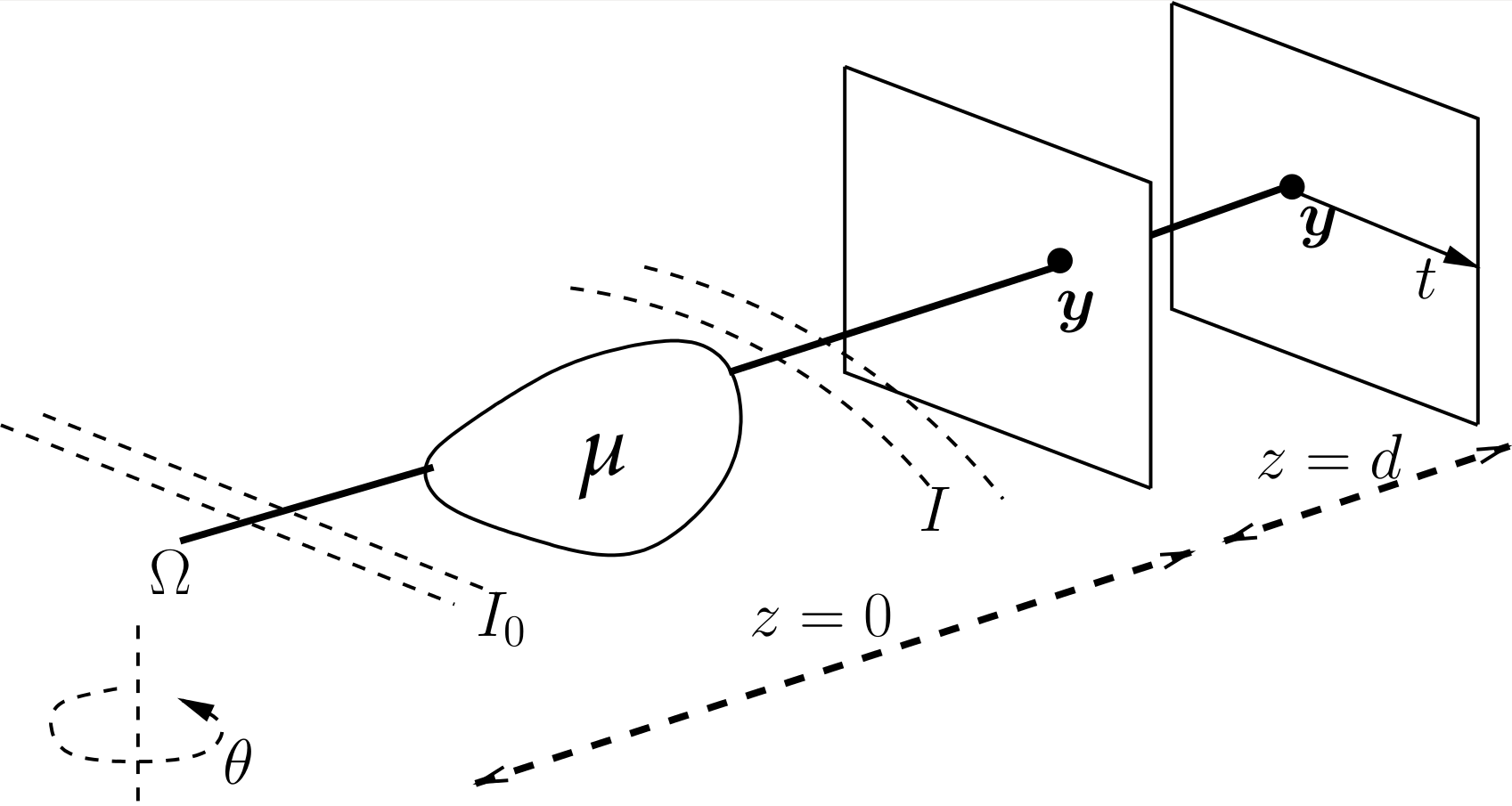
Since the sample is mainly composed by soft tissue determined by approximately one single material, all measurements were done using a phase contrast setup. In the present paper, the focus is on the mathematics of the phase contrast tomographic reconstruction, in order to enable the development of such a protocol in the future. To preliminarily test our techniques, we expose a stained [9] sample of fish eggs on the imaging beamline of the Brazilian Synchrotron Laboratory aiming at exploring the morphology of the Curimatã sample using conventional micro-tomography.
2 Mathematical Description
Mathematically, an intensity is measured at a given pixel on the plane detector, placed after the sample ; see Fig.1. Along the raypath , the paraxial wavefront of the scalar electromagnetic field is described by the transport intensity equation (tie)
| (1) |
where indicates the phase and is a point on the detector plane. A large class of methods for the phase-retrieval problem is summarized in the work of Burvall [1]. It is claimed that a general approximate solution of the tie (1) at the near contact plane is proportional to the thickness of the sample along – say – and must satisfy the following functional relation
| (2) |
with standing for the Laplacian operator and a constant depending on the phase coefficients and the distance . Here, is the incident wavefront at the sample. After taking the Fourier transform on the above equation, the approximate solution becomes
| (3) |
Operator indicates the operator described by Paganin, for a fixed . In this work, we are particularly interested in the operator and kernel described by
| (4) |
where stands for Fourier transformation,
| (5) |
For example, in the case of an object with a single material, the approximate solution was given by Paganin [3] with and . Taking , the solution of (2) is obtained using the inverse of the Radon Transform . For this case, there are several reconstruction algorithms able to invert the operator .
Phase-retrieval discussion starts with the assumption that the integration operation along the sample – through the raypath and hiting the detector at point – can be approximated by a mean value . That is
| (6) |
where denotes the support (thickness) of the sample along the ray parameterized by . Hence, the general strategy in the literature, as pointed out in the work of Burvall [1], is that is the approximate solution of the tie (1), which satisfies the following equation
| (7) |
First equality on the above equation comes from the standard Beer-Lambert law. Using properties of the Fourier transform, the kernel can be written on the detector domain as
| (8) |
Hence, obtaining the map is a straightforward numerical process by means of the Fast Fourier Transform. Here, the constant comes from a strong physical assumption on the sample, which either relates to a single or a double material. From (7), the approximation indicates that in some sense, should be minimized in . It is obvious, due to the Beer-Lambert law for absorption, that the solution of return as the Radon transform of the attenuation coefficient, which in turns implies that we are not restoring the phase at the plane .
3 Tikhonov Regularization versus Phase Retrieval
In the Schwartz space equipped with the norm , let us denote . We look for a map which is the best smooth approximation of the normalized map . Smoothness in the solution is evaluated by the use of a “roughness measurement” operator . This leads to the problem of finding a global minimizer of the following functional
| (9) |
with a regularization factor . Indeed, (9) is a standard Tikhonov regularization approach for the smoothed least squares solution . A typical definition for the functional , enforcing smoothness on the solution , is the following
| (10) |
The first order optimality condition for the unconstrained problem (9) is determined by the Euler-Lagrange equations, which in the case of (10), coincide with the following normal equations
| (11) |
where is the hermitian-adjoint operator of . Due to the fact that and , the optimality condition (11) becomes
| (12) |
which is essentially the same equation as (2), obtained by approximate phase retrieval methods, with . In this case, it means that the optimal regularization parameter is the one that obeys some physical assumption.
Proposition 1.
Proof.
Let us denote the function to be minimized by , with
| (14) |
The Fréchet derivative of nonlinear functionals and are presented in the Appendix, using . The action of the linear functional on each is determined by
| (15) |
Hence, if and only if satisfies the equation
| (16) |
which using becomes the same as (12). That is, the solution of the Paganin equation is a stationary point of the functional .
To prove that , satisfying (16), is a local minimizer, we have to show that the second Fréchet derivative , as a bilinear form, satisfies
| (17) |
(see [10]). The second Fréchet derivative of each functional and are presented in the Appendix. Form evaluated at a pair obeys
| (18) |
The second Fréchet derivative of , at the stationary point follows
| (19) |
The bilinear form at , acting on – after several cumbersome but elementary simplifications – will be given by
| (20) |
Since is bounded (due to the compactness of the object) function and will also be minorized by some constant, due to the fact that . Let us assume that . Using this fact, we can minorize (20)
| (21) |
To minorize the last integral, we use the fact for all such that , and with . Hence,
Expression between brackets in the above equation has a lower bound since has bounded variation. Now, (21) becomes
| (22) |
Since is twice continuously Fréchet-diferentiable, the Taylor expansion around gives
for all such that . Using (22) and we finally obtain as the local minimizer of . ∎
Notice that, as increases, the retrieved phase becomes a blurred version of the normalized image ; on the other hand, taking gives us the linear attenuation coefficient. Assuming that approximate phase-retrieval methods give a solution of the optimization problem (9), there are many numerical strategies to find an ideal parameter [2, 11] , e.g., the -curve [12]. Even though is strictly related to physical properties of the sample under investigation, the regularized solution (3) is the one maximizing the contrast of the solution. In fact, from the optimality condition (12), the following decreasing function
| (23) |
always attains a maximum curvature at an optimal point . This is true due to the property of the -curve[6], which states that a compromise must be taken between the minimization of and smoothness by operator through the plot of the curve . Hence, we consider as the optimal parameter satisfying
| (24) |
and being the curvature of the function with , defined by
| (25) |
with prime denoting derivative with respect to (subscript stands for frame since this is a process done by projections). Computing first and second derivatives from function is a straightforward process due to properties of the Fourier transform. In fact, since with from (3), it is easy to obtain
| (26) |
which implies that
| (27) |
with kernels defined in the frequency domain by equation (26). Computing the optimal with an optimization algorithm for one-dimensional functions (such as Newton’s method or bfgs) is fast since the evaluation of the curvature function depends only on Fourier transforms.
One of the main disadvantages of the Paganin filtering approach, is that each frame has to be processed individually in order to obtain a single filtered block of the raw data. From the new dataset, we extract two or three dimensional reconstructions using some inversion scheme. This is an extremely intensive computational process that can be done with a graphics processing unity to speed up calculations [13]. To avoid nested loops in a programming strategy of in-line phase retrieval method, we propose a filtering strategy directly on the sinogram. In fact, we can use the Lipschitz property of the exponential function
| (28) |
In our case, the unknown approximates the path integral of the sample – say – (i.e., the Radon transform of ) on pixel of the area detector. Therefore, minimization of implies minimization of due to (28). Therefore, minimization of implies minimization of . This is true because the Fréchet derivative of the function is the linear functional determined by
| (29) |
Hence, is a critical point of the functional since (first order optimality condition). Since is convex, must be a global minimizer. A proof of (29) is given in the appendix.
Another strategy for phase-retrieval, the so-called Fourier method obtained with Born or the Rytov approximation described in [14], claims that a solution is obtained using
| (30) |
with a suitable kernel described in [1]. The main difference of (30) and (3) is the filter action, which is performed after the log-normalization. In this sense, we look for a smooth function which is close to , i.e., a solution of the following regularized optimization problem
| (31) |
with a smoothing operator. The Euler-Lagrange equations for the above functional can be simplified considering the skew-adjoint operator (here, coincide with the axis, the horizontal axis for a given slice)
| (32) |
After taking Fourier transformations, we arrive at the optimal regularized solution
| (33) |
which is a filtering operation over the sinogram , i.e., . The retrieved sinogram obtained with (33) is similar to the Rytov-Born [14] approximated solutions for in-line phase retrieval tomography in the Fresnel regime. Both assume that phase coefficients are proportional, and also that which is true for the fish egg sample.
Proposition 2.
Proof.
In this particular case, the optimal parameter can be found as the one that maximizes the curvature of the function with
| (35) |
where stands for the second derivative on the ray axis (subscript stands for slice since this is a process done by sinograms). Curvature function is the same defined in (25), replacing by . As stated previously, a one-dimensional optimization algorithm can easily take advantage of the fast evaluation of the objection function through fast fourier transforms. For completeness, it is easy to note that
| (36) |
with being represented in the frequency domain through
| (37) |
The main difference for the in-line phase retrieval methods described by Proposition 2 relies on the evaluation of the difference
| (38) | |||||
| (39) |
We propose the following result for an upper bound estimate to function .
Proposition 3.
Proof.
Case is trivial since
Since and are positive operators, it is true from the triangle inequality that
| (40) | |||||
| (41) |
Last inequality holds since and . Due to Jensen’s inequality [15] we can majorize the second convolution integral of (41) to obtain
| (42) | |||||
| (43) | |||||
| (44) | |||||
| (45) |
Finally, using Parseval’s identity, each norm and is assymptotically bounded in variable by the factor because the maximum of and is one, in variables and , respectively. In this case,
| (46) |
is the final bound for the difference (38). ∎
It is important to note that the one-dimensional convolution integral with kernel applies over the axis, keeping fixed (the slice axis). On the other hand, the two-dimensional integral of the denominator - with kernel - applies for the entire domain of . To overcome the difficulty in comparing kernels and , let us introduce the operator
| (47) |
It is obvious that as and Fourier transforms results in . Returning to starting equation (2) and replacing by we arrive at an equation similar to (3) with a kernel defined in the frequency domain by
| (48) |
Now, it is easy to realize that .
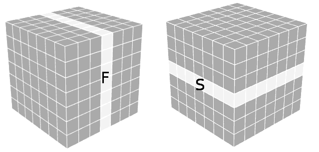
Asuming a cubic dataset with slices, rays and angles, it is easy to note that the computational complexity to apply a phase-retrieval strategy either by frames or slices on the entire cube, is . The disadvantage of using the frame-strategy is the need to restore the cubic dataset prior to reconstruction, while the slice-strategy can be easily included in the stacking reconstruction process. Figure 2 ilustrates the difference between filtering by frames and slices. Although they never provide identical filtered datasets, the difference is bounded by a small constant, as we show in Proposition 3.
The next Proposition provides a relation between our one-dimensional optimization strategy and the dispersion measure of the input data.
Proposition 4.
The optimal curvature parameter , which maximize the curvature of function defined in (35), is invertionally proportional to the cutoff frequency .
Proof.
We begin with definition (35) and use the fact that for all fixed, but arbitrary. Due to Parseval’s identity we obtain for large values of the cutoff frequency
| (49) | |||||
| (50) | |||||
| (51) | |||||
| (52) | |||||
| (53) |
Last equality is obtained using a straightforward integral calculation and a mean value of for some over the interval . It is easy to realize that function is asymptotically defined as so that
for an increasing sequence of cutoff frequencies . From the above inequality and since has an assymptotic behaviour with , the optimal curvature point from function determines an increasing sequence , as shown in Figure 3.
∎
A similar discussion applies for the two-dimensional case, changing kernel by . in the 2D frequency variable . Further strategies could be used, replacing operator in (31) by a generalized linear combination of first and second derivatives on the -axis in order to obtain smoother sinograms, i.e.,
| (54) |
In this case, the resulting differential equation, with his associated Fourier representation is
| (55) |
4 Regularized Filtered Backprojection Phase-Retrieval
The filtered backprojection inversion algorithm states that a given slice can be reconstructed from a sinogram through the following inversion formula
with the measured image data. Operator is the so-called backprojection operator, which is the adjoint of the Radon transform , i.e., the stacking operator over the family of x-rays passing through the sample. Operator is a low-pass filtering operator, acting on the variable , i.e., , for all . The complex computational part of the fbp algorithm is the computation of for all pixels in the region of interest . It is an algorithm with complexity with being the number of pixels for the reconstructed image. It was recently shown [16] that can be computed with complexity using a polar representation. In this case, it is possible to proof [17] that a dual formulation of the Fourier-slice theorem is also valid; it was refered as a backprojection-slice-theorem (bst). The theorem states that the Fourier of backprojection of any sinogram image can be computed in polar coordinates of the frequency domain using
with . Further details about the above formula can be found in [16]. The bst formula can be used to obtain an analytical solution of the standard Tikhonov regularization problem
| (56) |
with the smoothingself-adjoint operator defined as
| (57) |
In (56), we are looking for the best smooth approximation to the measured data. Here, is the space equiped with the norm. After exploring the Euler-Lagrange equations for the above optimization problem, we obtain the following representation in the frequency domain for the solution
| (58) |
The proof of the above equation can be found with details in [17], although using as an identity operator. Since is self-adjoint, the bst formula with further properties of the Fourier transform give us (58). We note that (58) is a regularized version of the Fourier-Slice-Theorem and can be used to obtain explicitly through any gridding strategy [18]. Applying (58) in the Fourier representation of we finally obtain a new representation for the reconstructed image ,
| (59) |
Equation (59) provides exactly the same reconstruction pattern as a typical filtered backprojection reconstruction algorithm, but with the phase-retrieval kernel acting on the sinogram . In fact, we can generalize our regularized strategy in the following representation
| (60) |
Now, is a family of solutions of the optimization problem (56), depending on the regularization parameter . The filter function is defined in (33). Our regularized solution (60) depends explicitly on the computation of the backprojection operator and either the bst formula, or different strategies could be used. Figure 4.a presents the family filter for three different values of , while 4.b the lowpass action of the filter on the input sinogram .
| (a) | (b) |
|---|---|
5 Experimental validation
The curimatã fishegg sample, described in the Introduction, was exposed to the imaging beamline from the Brazilian synchrotron light source, using only 200 angles. Figure 5 presents a slice reconstructed using the transmission expectation maximization algorithm [19]. It is clear that there is a small absorption of the sample and low contrast. Hence, image segmentation is nearly impossible. Well known image segmentation techniques, commonly implemented in commercial software for 3D visualization and data analysis, grossly failed in this case of study. Region-based segmentation methods [20] use the pixel grayscale to separate the image into different regions and threshold method works well with a bimodal distribution of grayscales, which is clearly not seen in this case, see Figure 6.(a). Watershed, a more robust region-based segmentation method, comes from the geological idea of valleys and ridges identification, which are related to the grey level of the image. In this specific case, since there is a high grayscale variation observed between neighbouring pixels - see Figure 6.(b) - this methodology oversegment the image, creating many small different regions.
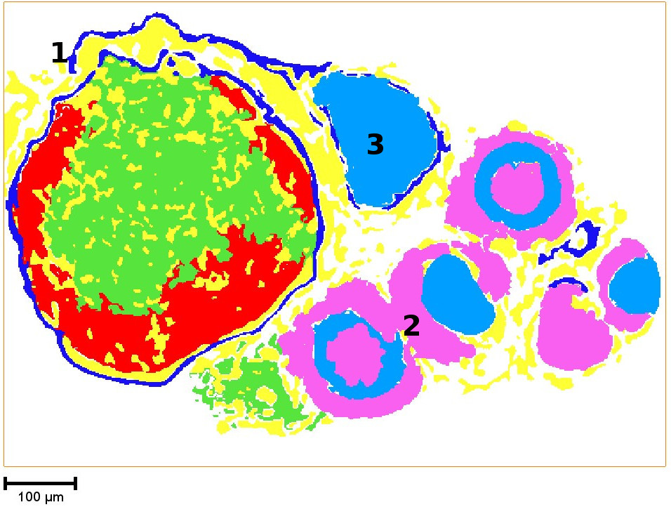
The reconstruction using the expectation maximization algorithm with the filtered sinogram - using kernel is presented in Fig.7, where now contrast is considerably higher if compared with the unfiltered result of Fig.5. Image segmentation of the new image is now much easier, and is presented in Fig.8. Here, as the image contrast was enhanced, threshold tool was enough to separate most of the regions (e.g. contour region 1 and 2 of Figure 7). However, other regions still present high differences in grayscale (e.g. region 3 of Figure 7), and a combination of edge detection and fill interior tools had to be applied. The optimal value for was obtained using the curvature strategy described in Section 3.
| (a) | (b) |
|---|---|
| (a) | (b) |
|---|---|
| (a) | (b) |
|---|---|
 |
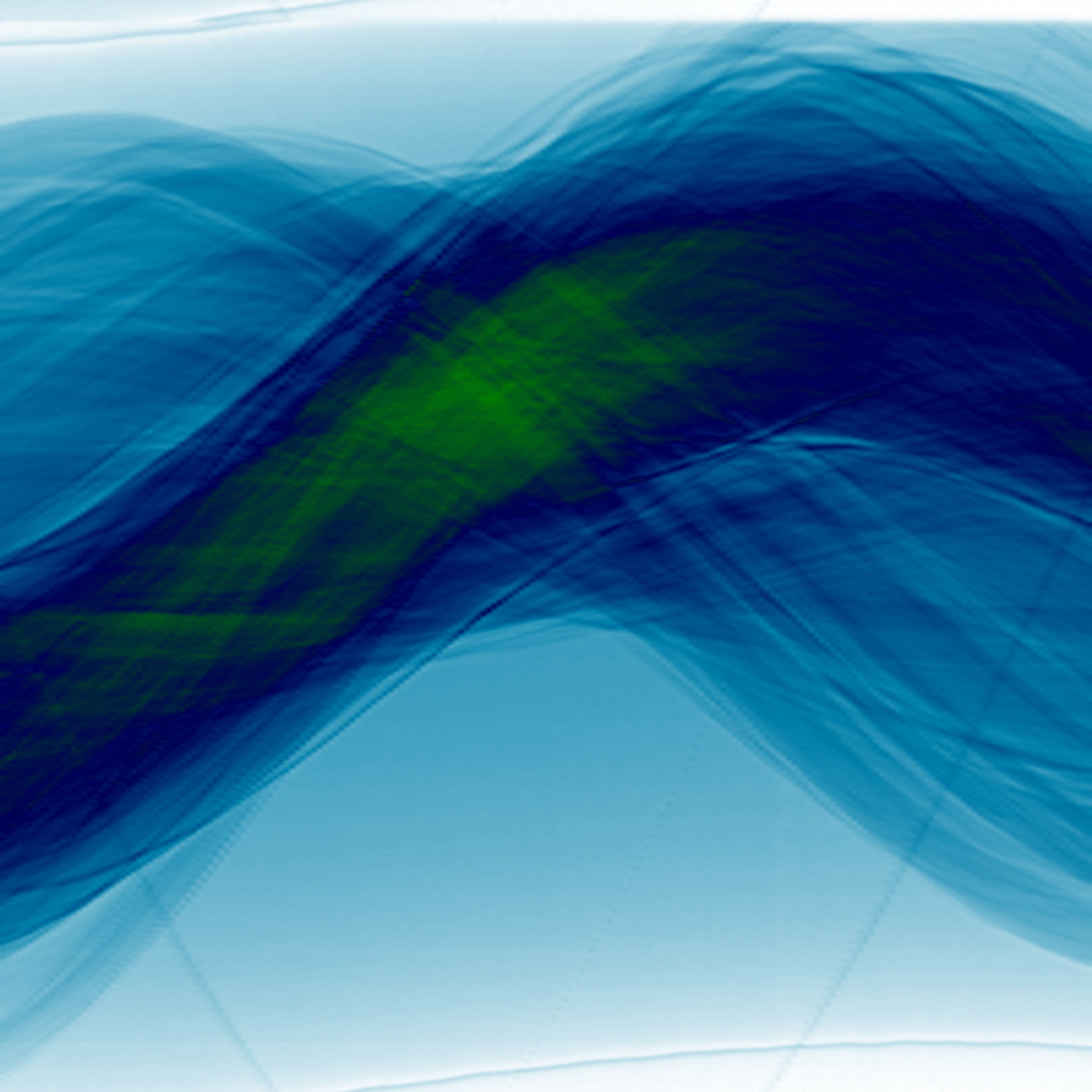 |
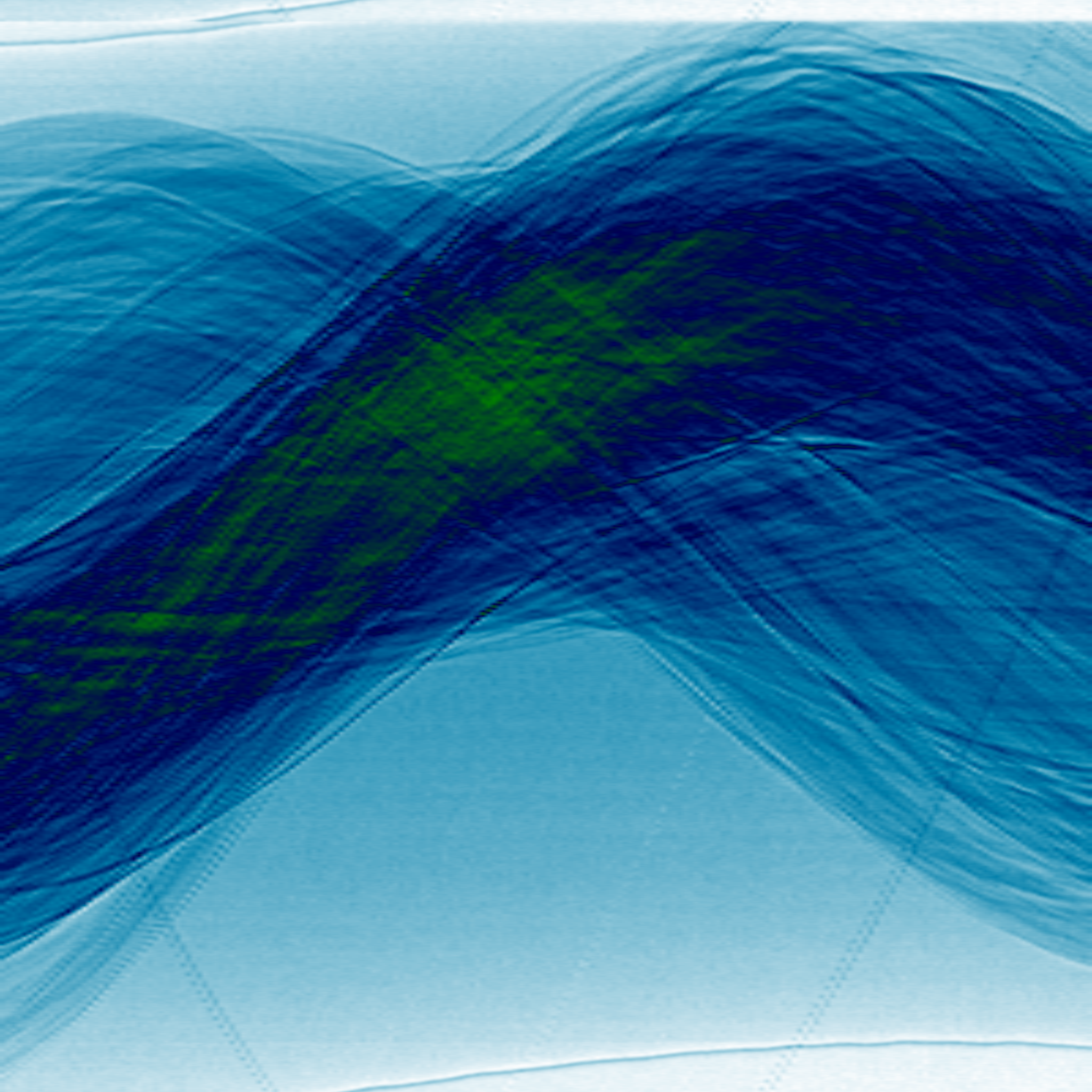
Two filtered sinograms are depicted in Figure 10 comparing the regularization strategy by frames and by slice. Although the sinograms are not equal, their difference is bounded by , as shown in Table 1. Also, Table 1 presents the optimal values using the one-dimensional curvature strategy.
| Optimal (meters) | ||
|---|---|---|
| Frames | ||
| Slice |
To validate the numerical curvature strategy, we expose the sample at 29 different distances obtaining a normalized sequence of frames ,
A small distance indicates a near-contact propagation while for long distances like , the phase becomes more visible. Each satisfies the approximation (2) with a parameter that depends linearly on the distance [21, 1], i.e.,
| (61) |
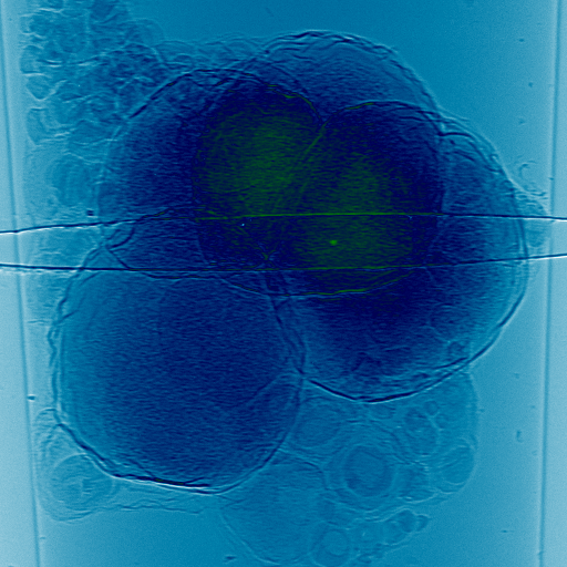
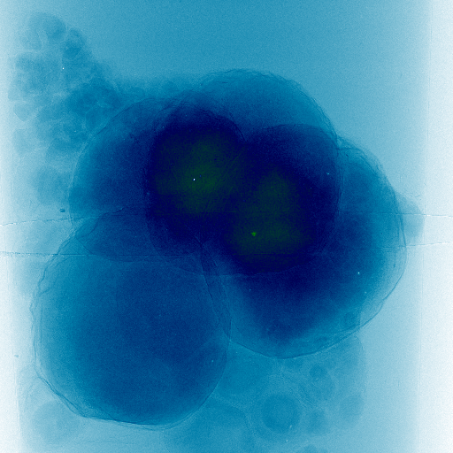
where is the wavelength. First and last frame are presented in Figure 11, where edge enhancement is clearly visible for high distances in the Fresnel regime.
| (a) | (b) |
|---|---|
 |
 |
According to our numerical scheme, we can restore an approximation of computing the point of maximum curvature of the function in (24), i.e,
The sequence as a function of , obtained for this experiment, is presented in Figure 12.a. Since is not linear with respect to , as predicted by theory, we investigate the effect of changing the cutoff-frequency defined as
| (62) |
where is the sampling rate on the square domain for . Here, is a positive constant and the mesh for the two-dimensional frequency variable is such that . Number is proportionally inverse to the number , as given in Proposition 4. In this case, The blinded restoration (i.e., without knowing the true value of ) using the optimization strategy presented in the plot of Figure 12.a was obtained using .
| (a) | (b) |
|---|---|
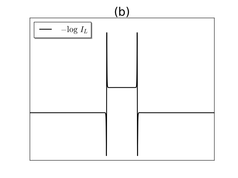
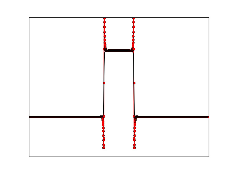
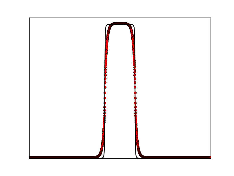
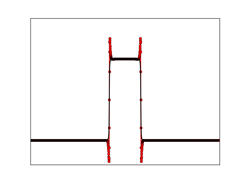
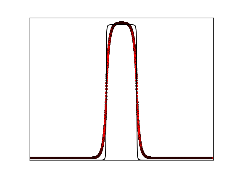
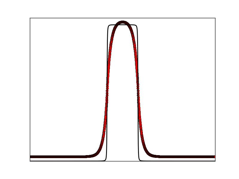
In order to investigate the effect of variable , which defines the cutoff-frequency (62), we investigate our approach using a one-dimensional example. Let be the rectangular function representing the electronic density, i.e., . We can approximate using the following approximation for the function, , i.e.,
| (63) |
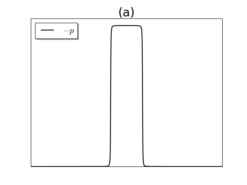
We have used and as depicted in Figure 13.a; in this case, the propagation is determined by
| (64) | |||||
| (65) |
with derivatives known a priori. Function is shown in Figure 13.b using value with mm, , , and .
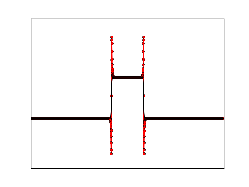
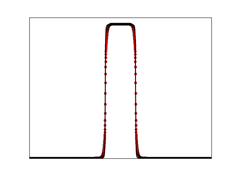
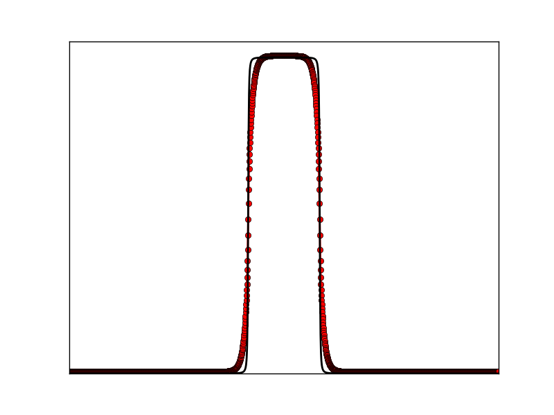
Let us denote the recovered signal as . Some examples with different values of the pair are presented in Figure 14. Columns (a), (b) and (c) are for constant values of , and , respectively. Rows are varying from top to bottom with , and .
| (a) | (b) | (c) |
|---|---|---|
|
|
|
|
|

|
|
|
|
Taking the result of Figure 14, we observe (due to the intermediate value Theorem) that exist a value of between 0.00163522409163 and 0.163522409163 that restore the signal . However, the restored value for an arbitrary value of possibly does not have any relation with the one obtained by the optimization strategy. Let be the sequence of values for , which controls the cutoff-frequency (62). The sequence of restored values is presented in Figure 15.a, where it is clear that exist a value of such that .
Now, computing the right for each distance value using a force brute algorithm give us the sequence depicted in Figure 14.b. For an increasing value of distance, behaves linearly as predicted by theory and presented in Figure 14.c and 14.d. It is important to note that versus behave as predicted in Proposition 4, i.e., .
| (a) | (b) |
| (c) | (d) |
In the last experiment we expose a sample made of a thick kapton tape to the imaging beamline, using angles and a distance of mm, each with an exposure time of 3 seconds. The idea was to test the one-dimensional optimization algorithm by frames. A given slice reconstructed with the expectation algorithm maximization is presented in Figure 16. The constrast is considerably poor inside the sample due to low absorption of the beam on the sample. Applying the one-dimensional strategy by frames with , we find an optimal , resulting in the reconstruction shown in Figure 17. According to the database from nist [22], since kapton is a polyimide film with that and we obtain the theoretical given by , which is satisfactory to the obtained by our algorithm.
6 Conclusion
In this manuscript we have described a strong relation between in-line phase retrieval methods and a Tikhonov regularization for the imaging of light samples in the Fresnel regime. Considered as a regularized variational problem in an appropriate functional space, we provide a simple one-dimensional algorithm, which aims to restore the physical parameter , usually given empirically, and needed to restore the phase in the near contact regime. An automatic algorithm capable to restore the right convolution parameter improve quality of image segmentation, which depends on the contrast of the reconstructed image. However, the one-dimensional algorithm relates directly to the cutoff-frequency , also inversely proportional to the dispersion of the measured data. Even though and are also related, we claim that exist an optimal for which the 1d algorithm provide a best approximation of the appropriate physical parameter . An algorithm to find was out of the scope of this manuscript.
Appendix A Appendix
A.1 Fréchet Derivatives
Let be the usual norm. We compute the Fréchet derivative of the following nonlinear functionals and , acting on a function with :
| (66) |
and
| (67) |
Function :
First Derivative:
For all , the error is given by
Since for we finally get
| (68) |
The definition of the Fréchet derivative comes from (68) since
Second Derivative:
Second Fréchet derivative is a bilinear operator acting on a pair as
| (69) |
Using the same reasoning, we can easily verify that
The approximation was used to obtain the above formula.
Function :
First Derivative:
Let us consider the following operator
which has Fréchet derivative given by , acting as a linear operator in the following sense
Now, our functional is related to as
or
Hence, using the chain rule in the Fréchet sense,
Since is a also a composition, its easy to realize that , therefore
with the identity operator. Replacing we finally obtain
As a linear operator, the action of is given by
| (70) |
Second Derivative:
This derivative was obtained using the approximation in the definition (69).
Acknowledgments
Staining of the Curimatã fish egg sample was kindly provided by Juliana Martins S. Silva. We also thank Nikolay Koshev and João C. Cerqueira for helping with the implementation of some of the methods described in this manuscript.
References
- [1] Anna Burvall, Ulf Lundström, Per AC Takman, Daniel H Larsson, and Hans M Hertz. Phase retrieval in x-ray phase-contrast imaging suitable for tomography. Optics express, 19(11):10359–10376, 2011.
- [2] H Rositi, C Frindel, M Wiart, M Langer, C Olivier, F Peyrin, and D Rousseau. Computer vision tools to optimize reconstruction parameters in x-ray in-line phase tomography. Physics in medicine and biology, 59(24):7767–7775, 2014.
- [3] David Paganin, SC Mayo, Tim E Gureyev, Peter R Miller, and Steve W Wilkins. Simultaneous phase and amplitude extraction from a single defocused image of a homogeneous object. Journal of microscopy, 206(1):33–40, 2002.
- [4] David Paganin. Coherent X-ray optics. Number 6. Oxford University Press on Demand, 2006.
- [5] P Jonas and AK Louis. A sobolev space analysis of linear regularization methods for ill-posed problems. Journal of Inverse and Ill-Posed Problems, 9(1):59–74, 2001.
- [6] Per Christian Hansen. Analysis of discrete ill-posed problems by means of the l-curve. SIAM review, 34(4):561–580, 1992.
- [7] RH Lowe-McConnell and RH Lowe-McConnell. The neotropical fauna fish (in portuguese). Estudos ecológicos de comunidades de peixes tropicais (RH Lowe-McConnell, ed.). EDUSP, São Paulo, pages 129–168, 1999.
- [8] Daniel M Cohen. How many recent fishes are there? California Academy of Sciences, 1970.
- [9] Juliana Martins de S e Silva, Irene Zanette, Peter B Noël, Mateus B Cardoso, Melanie A Kimm, and Franz Pfeiffer. Three-dimensional non-destructive soft-tissue visualization with x-ray staining micro-tomography. Scientific reports, 5, 2015.
- [10] David G Luenberger. Optimization by vector space methods. John Wiley & Sons, 1969.
- [11] Elias Salomão Helou and Lucas Eduardo Azevedo Simões. A new parameter choice method for inverse problems with poisson noise. In XXV SIBGRAPI - Conference on Graphics, Patterns and Images, 2014.
- [12] Peter R Johnston and Ramesh M Gulrajani. Selecting the corner in the l-curve approach to tikhonov regularization. Biomedical Engineering, IEEE Transactions on, 47(9):1293–1296, 2000.
- [13] FRNC Maia, Alastair MacDowell, Stefano Marchesini, Howard A Padmore, Dula Y Parkinson, Jack Pien, Andre Schirotzek, and Chao Yang. Compressive phase contrast tomography. In SPIE Optical Engineering+ Applications, pages 78000F–78000F. International Society for Optics and Photonics, 2010.
- [14] Timur E Gureyev, Timothy J Davis, Andrew Pogany, Sheridan C Mayo, and Stephen W Wilkins. Optical phase retrieval by use of first born-and rytov-type approximations. Applied optics, 43(12):2418–2430, 2004.
- [15] Tristan Needham. A visual explanation of jensen’s inequality. The American mathematical monthly, 100(8):768–771, 1993.
- [16] Eduardo X. Miqueles and Elias S. Helou. Fast backprojection operator for synchrotron tomographic data. In European Conference on Mathematics for Industry. Springer, 2014.
- [17] Nikolay Koshev, Elias S. Helou, and Eduardo X. Miqueles. Fast backprojection techniques for high resolution tomography. https://arxiv.org/pdf/1608.03589v1.pdf, 2016.
- [18] F Marone and M Stampanoni. Regridding reconstruction algorithm for real-time tomographic imaging. Journal of synchrotron radiation, 19(6):1029–1037, 2012.
- [19] K Lange. Convergence of em image algorithms with gibbs reconstruction smoothing. IEEE Transactions On Medical Imaging, 9(4):439–446, 1990.
- [20] Muhammad Waseem Khan. A survey: Image segmentation techniques. International Journal of Future Computer and Communication, 3(2):89, 2014.
- [21] T Weitkamp, D Haas, D Wegrzynek, and A Rack. Ankaphase: software for single-distance phase retrieval from inline x-ray phase-contrast radiographs. Journal of synchrotron radiation, 18(4):617–629, 2011.
- [22] X Nist. ray photoelectron spectroscopy database, 1997.