Analytical results for a stochastic model of gene expression with arbitrary partitioning of proteins

Hugo Tschirhart1,2,3 & Thierry Platini4 1 University of Luxembourg, Physics and Materials Science Research Unit, Avenue de la FaΓ―encerie 162a, L-1511 Luxembourg, Luxembourg
2 Groupe de Physique Statistique, Institut Jean Lamour (CNRS UMR 7198), Université de Lorraine Nancy, B.P. 70239, F54506 Vandoeuvre-lès-Nancy Cedex, France,
3 Doctoral College for the Statistical Physics of Complex Systems, Leipzig-Lorraine-Lviv-Coventry (𝕃4superscript𝕃4{\mathbb{L}}^{4})
4 Applied Mathematics Research Center, Coventry University, Coventry, CV1 5FB, England,
thierry.platini@coventry.ac.uk
Abstract

In biophysics, the search for analytical solutions of stochastic models of cellular processes is often a challenging task. In recent work on models of gene expression, it was shown that a mapping based on partitioning of Poisson arrivals (PPA-mapping) can lead to exact solutions for previously unsolved problems. While the approach can be used in general when the model involves Poisson processes corresponding to creation or degradation, current applications of the method and new results derived using it have been limited to date. In this paper, we present the exact solution of a variation of the two-stage model of gene expression (with time dependent transition rates) describing the arbitrary partitioning of proteins. The methodology proposed makes full use of the the PPA-mapping by transforming the original problem into a new process describing the evolution of three biological switches. Based on a succession of transformations, the method leads to a hierarchy of reduced models. We give an integral expression of the time dependent generating function as well as explicit results for the mean, variance, and correlation function. Finally, we discuss how results for time dependent parameters can be extended to the three-stage model and used to make inferences about models with parameter fluctuations induced by hidden stochastic variables.

pacs:
87.10.Ca, 87.10.Mn, 87.18.Cf, 87.18.Tt

1 Introduction

Gene expression is the biological process by which information from a gene is used to synthesize RNA macromolecules and proteins. With a few exceptions, until the 1990s, this process was commonly understood from β€œa deterministic viewpoint” [1, 2]. Since then, the combination of experimental and theoretical approaches has clarified that gene expression is often stochastic in nature (see [3, 4, 5, 6, 7] for review articles). The effect of fluctuations (noise) is usually limited when we are dealing with large numbers of molecules [8]. In cells however, wherein genes and mRNAs are often present in low numbers, stochasticity has an important role on cellular functions. The importance of fluctuations [9, 10, 11, 12, 13, 14, 15] can be illustrated by the observation that, amongst a genetically identical population in a homogenous environment, cell-to-cell variations in gene expression can result in phenotypic heterogeneity.

There exists various mechanisms, some more complex than others, allowing cells to tame and exploit randomness [16]. In order to unveil those processes, research efforts are directed on both experimental [17, 18, 19, 20] and theoretical fronts [21, 22, 23, 24, 25, 26, 27, 28, 29]. Collaborations between biologists, physicists and mathematicians aim to reveal the conditions under which transcriptional noise may, or may not, cascade to affect downstream genetic products.

The two stage and three stage models [30, 31, 32, 33, 34] give a minimalist description of the simplest yet non-trivial biological processes leading to gene expression. The two-stage model includes only transcription and translation processes, while the three-stage model also incorporates free and repressed states of the DNA promoter region. Analytical techniques and results [35, 36, 37] for the previously mentioned processes are the cornerstone for further theoretical developments. These models are the elementary bricks allowing for the construction of more complex reaction networks including non-exponential waiting times, transcriptional burst, feedback loops et cetera [38, 39, 40, 41, 42]. Even when it is possible to derive the exact mean and variance of protein and mRNA numbers, obtaining an exact closed-form expression for the generating function is often a challenging problem. The two-stage model is a perfect example. It has been the subject of numerous studies since the paper of Thattai and Oudenaarden [40] in 2001. The model presents linear propensities so that all moments can be derived exactly. Such problems (like the one considered in this paper) are said to be β€œexactly solvable”. Nevertheless, the exact generating function for the two stage model [37] was obtained only after ten years of extensive theoretical and experimental studies.

The search for exact solutions is often challenging because a small variation of a model’s definition can make analytical results unattainable. Typically methods aiming for a full characterisation of a given process (beyond results for the mean and variance), focus on the master equation approach and its partner equation for the generating function. Once the generating function is obtained, all moments are in principle known: given by successive derivatives. This approach can provide insights into different limiting cases and into the behaviour of the distribution in different regions of parameter space. It is important to mention that analytical results (for the probability distribution) have been obtained for a class of models such as monomolecular reactions systems [61] or deficiency zero networks [62, 63]. Unfortunately, once outside these classes there exists no systematic analytical recipe applicable independently of a model’s structure. Research efforts are naturally turning towards numerical simulations which though powerful β€œbring no intuition into the underlying […] interactions” [40]. To reach a better understanding one needs to investigate the joint distribution of mRNA and proteins, as well as temporal data, beyond the two-time autocorrelation function. As research progresses, emphasis is given to real time measurements with the hope to β€œexpose the true cell dynamics buried in the average” [23]. Nowadays experimental advances allow for the count of individual molecules over time [43, 44, 45, 46] highlighting the need for both time-dependent and steady-state theoretical results .

In recent work, the partitioning of Poisson arrivals [47] was invoked to map Poisson processes to simple biological switches. This method is based on the separation of creation events (mRNA creation or protein creation) into independent groups. When applicable, this procedure leads to a mapping between creation/degradation process and a simple two-states biological switch. Applied to the two-stage model, this method led to the time dependent protein distributions [47] using already known results [21, 18, 36] for mRNA distributions in models with promoter-based regulation. The PPA-mapping needs, however, to be applied with care. It is important to warn the reader that, in a given model, not all creation/degradation process can be mapped onto a biological switch. For the PPA-mapping to apply, one needs to be able to partition a given creation event into independent processes. And for a given model, this will depend on upstream regulation of the creation/degradation process under consideration. This restriction is strong and appears as a serious limitation of the mapping applicability. We therefore need a more systematic way to use the PPA-mapping. As it is, the PPA mapping, can only be applied on models presenting a mixture of zero and first order reactions. It is unclear as if and how this method can be used or adapted to study models in the presence of feedback. In the simplest model describing bursty mRNA production, a variation of PPA mapping leads to an alternative derivation of the mRNA generating function [48]. But so far, this method has not been the subject of much attention and few models have been solved using this approach.

In direct connection with the applicability question of the PPA mapping is the inverse problem: Assuming the arbitrary partition of a creation event into two β€˜types’ (type 111 and type 222), the latter process being itself regulated by an upstream mechanism, what correlation (between 111 and 222) should we expect? Is the correlation bounded? Does it vanish under particular conditions? Also, it is of experimental interest, to search for ways to infer the protein levels of a given type using measurement data on the other.

The model and methodology proposed in this paper were designed to (1) study correlations induced by the arbitrary partition of proteins arrival and (2) obtain the generating function making full use of the idea implicit in the PPA-mapping. The process we consider appears to be a simplified version of mechanisms involved in alternating splicing processes allowing a single gene to code for multiple proteins. With alternating splicing, a particular pre-mRNA can lead to different messenger RNAs, each being responsible for the production of isoform proteins (differing in their amino acid sequence). Results recently published in [49] focused on both bursty and constitutive pre-mRNA creation. One should mention that alternating splicing is far from being rare. Many genes have multiple splicing patterns [50, 51, 52] and numerous examples confirm that alternating splicing contributes to the development of cancer (see [53] and [54] for review articles). Our goal is to obtain the time dependent solution of the proposed model in term of the generating function. Our method is based on the construction of different mappings. Each transformation aims to reduce the study of a given model to the analysis of a simpler one. After a succession of transformations the problem is condensed to the study of two-state biological switches. The nesting between models and reduced models is reflected in a set of relations between generating functions. This hierarchy allows us to derive relations between mean numbers and higher order moments. We show that the PPA mapping allows us to consider arbitrary time dependent transition rates. Other studies such as [58, 59] and [60] have considered explicit time dependent parameters to investigate the effect of upstream hidden dynamics on downstream populations. Here, we obtain the time dependent generating function without solving any complicated differential equation but rather a simple first order equation (with time dependent coefficients). Accessing analytical results for time dependent coefficient provides a way to tackle models with noisy transition rates induced by hidden stochastic variables. In this paper, we show how results for the mean and correlations for time dependent model can be used to access the solution for the three-stage model.

The paper is organised as follows. In section (2.1), we start with the presentation of the model under consideration. We give the master equation governing the evolution of the probability distribution and present the solution of the first order moments. In section (2.2), we define the generating function, and outline the three different steps defining our method. Step 111 and 333 both describe the transformation under the PPA-mapping at different stages of the derivation. The intermediate step 222 defines the decomposition of a given process over all possible histories. Each step is detailed in sections (2.4), (2.5) and (2.6). The succession of transformations takes us relatively far away from the solution of the original problem. To proceed further, we give in section (2.7), the probability associated to each relevant histories. Finally, the time dependent generating function is presented in section (3), where our result is generalised to arbitrary partition numbers. We show how for some particular cases our results match the known solution for the two-stage model (see reference [37] and [47]). Finally we discuss how to use results for time dependent parameters to extend this work to the three-stage model and others processes including additional random variables.

2 Theory

2.1 The model

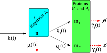
The model under consideration describes the stochastic evolution of protein numbers in a variation of the two-stage model, for which proteins are arbitrarily separated into two groups (𝒫1subscript𝒫1{\cal P}_{1} and 𝒫2subscript𝒫2{\cal P}_{2}). Note that our results will be easily generalized to an arbitrary number of protein types. We denote by π’œπ’œ{\cal A} the upstream molecule regulating proteins production (see Figure (1)). Time dependent transition rates for proteins production and degradation are respectively written qj​(t)subscriptπ‘žπ‘—π‘‘q_{j}(t) and Ξ³j​(t)subscript𝛾𝑗𝑑\gamma_{j}(t) (with j=1,2𝑗12j=1,2). The level of regulator π’œπ’œ{\cal A} is itself governed by the transition rates k​(t)π‘˜π‘‘k(t) and μ​(t)πœ‡π‘‘\mu(t), respectively associated to creation and degradation (see table (1)). Because the method presented in this paper invokes mappings to other processes, it is convenient to refer to the original model as model-0.
Refer to caption
Figure 1: The original model (model-0): Two types of proteins (𝒫1subscript𝒫1{\cal P}_{1} and 𝒫2subscript𝒫2{\cal P}_{2}) are regulated by an upstream molecule π’œπ’œ{\cal A}. Transition rates for protein production and degradation are respectively written qj​(t)subscriptπ‘žπ‘—π‘‘q_{j}(t) and Ξ³j​(t)subscript𝛾𝑗𝑑\gamma_{j}(t) (with j=1,2𝑗12j=1,2), while k​(t)π‘˜π‘‘k(t) and μ​(t)πœ‡π‘‘\mu(t) denote production and degradation rates for regulator π’œπ’œ{\cal A}.

The state of the system is, at any time, characterised by the numbers n𝑛n, m1subscriptπ‘š1m_{1} and m2subscriptπ‘š2m_{2}, of molecules π’œπ’œ{\cal A} and proteins 𝒫1subscript𝒫1{\cal P}_{1} and 𝒫2subscript𝒫2{\cal P}_{2} respectively. We write Pn,m1,m2​(t)subscript𝑃𝑛subscriptπ‘š1subscriptπ‘š2𝑑P_{n,m_{1},m_{2}}(t) the probability distribution of state (n,m1,m2)𝑛subscriptπ‘š1subscriptπ‘š2(n,m_{1},m_{2}). We should keep in mind that the latter quantity is conditional on the initial state. In particular, we will consider P0,0,0​(t=0)=1subscript𝑃000𝑑01P_{0,0,0}(t=0)=1. Further down in this paper we will explain how the latter initial condition is imposed by the initial state of the reduced model resulting from successive mappings. In order to consider other initial states, an extension of the proposed method is needed. This procedure would add an extra layer of complexity to the work presented here and is not discussed further in this paper. The probability distribution is governed by the master equation

dd​t​Pn,m1,m2𝑑𝑑𝑑subscript𝑃𝑛subscriptπ‘š1subscriptπ‘š2\displaystyle\frac{d}{dt}P_{n,m_{1},m_{2}} =\displaystyle= k​(t)​[Pnβˆ’1,m1,m2βˆ’Pn,m1,m2]π‘˜π‘‘delimited-[]subscript𝑃𝑛1subscriptπ‘š1subscriptπ‘š2subscript𝑃𝑛subscriptπ‘š1subscriptπ‘š2\displaystyle k(t)[P_{n-1,m_{1},m_{2}}-P_{n,m_{1},m_{2}}]
+\displaystyle+ μ​(t)​[(n+1)​Pn+1,m1,m2βˆ’n​Pn,m1,m2]πœ‡π‘‘delimited-[]𝑛1subscript𝑃𝑛1subscriptπ‘š1subscriptπ‘š2𝑛subscript𝑃𝑛subscriptπ‘š1subscriptπ‘š2\displaystyle\mu(t)[(n+1)P_{n+1,m_{1},m_{2}}-nP_{n,m_{1},m_{2}}]
+\displaystyle+ q1​(t)​n​[Pn,m1βˆ’1,m2βˆ’Pn,m1,m2]subscriptπ‘ž1𝑑𝑛delimited-[]subscript𝑃𝑛subscriptπ‘š11subscriptπ‘š2subscript𝑃𝑛subscriptπ‘š1subscriptπ‘š2\displaystyle q_{1}(t)n[P_{n,m_{1}-1,m_{2}}-P_{n,m_{1},m_{2}}]
+\displaystyle+ q2​(t)​n​[Pn,m1,m2βˆ’1βˆ’Pn,m1,m2]subscriptπ‘ž2𝑑𝑛delimited-[]subscript𝑃𝑛subscriptπ‘š1subscriptπ‘š21subscript𝑃𝑛subscriptπ‘š1subscriptπ‘š2\displaystyle q_{2}(t)n[P_{n,m_{1},m_{2}-1}-P_{n,m_{1},m_{2}}]
+\displaystyle+ Ξ³1​(t)​[(m1+1)​Pn,m1+1,m2βˆ’m1​Pn,m1,m2]subscript𝛾1𝑑delimited-[]subscriptπ‘š11subscript𝑃𝑛subscriptπ‘š11subscriptπ‘š2subscriptπ‘š1subscript𝑃𝑛subscriptπ‘š1subscriptπ‘š2\displaystyle\gamma_{1}(t)[(m_{1}+1)P_{n,m_{1}+1,m_{2}}-m_{1}P_{n,m_{1},m_{2}}]
+\displaystyle+ Ξ³2​(t)​[(m2+1)​Pn,m1,m2+1βˆ’m2​Pn,m1,m2].subscript𝛾2𝑑delimited-[]subscriptπ‘š21subscript𝑃𝑛subscriptπ‘š1subscriptπ‘š21subscriptπ‘š2subscript𝑃𝑛subscriptπ‘š1subscriptπ‘š2\displaystyle\gamma_{2}(t)[(m_{2}+1)P_{n,m_{1},m_{2}+1}-m_{2}P_{n,m_{1},m_{2}}].

At this point, it is premature to solve the full master equation, and we start by deriving equations for mean population numbers. Let us denote ⟨π’ͺ⟩delimited-⟨⟩π’ͺ\langle{\cal O}\rangle the average of the observable π’ͺπ’ͺ{\cal O}, given by βˆ‘n,m1,m2π’ͺ​(n,m1,m2)​Pn,m1,m2subscript𝑛subscriptπ‘š1subscriptπ‘š2π’ͺ𝑛subscriptπ‘š1subscriptπ‘š2subscript𝑃𝑛subscriptπ‘š1subscriptπ‘š2\sum_{n,m_{1},m_{2}}{\cal O}(n,m_{1},m_{2})P_{n,m_{1},m_{2}}. For mean numbers we derive the equations:

dβ€‹βŸ¨n⟩d​t𝑑delimited-βŸ¨βŸ©π‘›π‘‘π‘‘\displaystyle\frac{d\langle n\rangle}{dt} =\displaystyle= k​(t)βˆ’ΞΌβ€‹(t)β€‹βŸ¨n⟩,π‘˜π‘‘πœ‡π‘‘delimited-βŸ¨βŸ©π‘›\displaystyle k(t)-\mu(t)\langle n\rangle, (2)
dβ€‹βŸ¨mj⟩d​t𝑑delimited-⟨⟩subscriptπ‘šπ‘—π‘‘π‘‘\displaystyle\frac{d\langle m_{j}\rangle}{dt} =\displaystyle= qj​(t)β€‹βŸ¨nβŸ©βˆ’Ξ³j​(t)β€‹βŸ¨mj⟩,j=1,2.formulae-sequencesubscriptπ‘žπ‘—π‘‘delimited-βŸ¨βŸ©π‘›subscript𝛾𝑗𝑑delimited-⟨⟩subscriptπ‘šπ‘—π‘—12\displaystyle q_{j}(t)\langle n\rangle-\gamma_{j}(t)\langle m_{j}\rangle,\ \ j=1,2. (3)

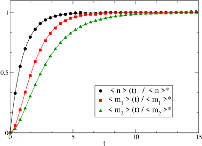
If we restrict ourself to the well known case of constant reaction rates, with ⟨nβŸ©β€‹(t=0)=⟨mjβŸ©β€‹(t=0)=0delimited-βŸ¨βŸ©π‘›π‘‘0delimited-⟨⟩subscriptπ‘šπ‘—π‘‘00\langle n\rangle(t=0)=\langle m_{j}\rangle(t=0)=0, the solutions of these equations are:

⟨nβŸ©β€‹(t)⟨nβŸ©βˆ—delimited-βŸ¨βŸ©π‘›π‘‘superscriptdelimited-βŸ¨βŸ©π‘›\displaystyle\frac{\langle n\rangle(t)}{\langle n\rangle^{*}} =\displaystyle= (1βˆ’eβˆ’ΞΌβ€‹t),1superscriptπ‘’πœ‡π‘‘\displaystyle\left(1-e^{-\mu t}\right), (4)

and

⟨mjβŸ©β€‹(t)⟨mjβŸ©βˆ—={1βˆ’1Ξ³jβˆ’ΞΌβ€‹(Ξ³j​eβˆ’ΞΌβ€‹tβˆ’ΞΌβ€‹eβˆ’Ξ³j​t),Ξ³j/ΞΌβ‰ 11βˆ’(1+μ​t)​eβˆ’ΞΌβ€‹t,Ξ³j/ΞΌ=1,delimited-⟨⟩subscriptπ‘šπ‘—π‘‘superscriptdelimited-⟨⟩subscriptπ‘šπ‘—cases11subscriptπ›Ύπ‘—πœ‡subscript𝛾𝑗superscriptπ‘’πœ‡π‘‘πœ‡superscript𝑒subscript𝛾𝑗𝑑subscriptπ›Ύπ‘—πœ‡111πœ‡π‘‘superscriptπ‘’πœ‡π‘‘subscriptπ›Ύπ‘—πœ‡1missing-subexpression\frac{\langle m_{j}\rangle(t)}{\langle m_{j}\rangle^{*}}=\left\{\begin{array}[]{cc}1-\frac{1}{\gamma_{j}-\mu}(\gamma_{j}e^{-\mu t}-\mu e^{-\gamma_{j}t}),&\gamma_{j}/\mu\neq 1\\ 1-(1+\mu t)e^{-\mu t},\ \gamma_{j}/\mu=1,\end{array}\right. (5)

with the stationary values ⟨nβŸ©βˆ—=k/ΞΌsuperscriptdelimited-βŸ¨βŸ©π‘›π‘˜πœ‡\langle n\rangle^{*}={k}/{\mu} and ⟨mjβŸ©βˆ—=k​qj/μ​γjsuperscriptdelimited-⟨⟩subscriptπ‘šπ‘—π‘˜subscriptπ‘žπ‘—πœ‡subscript𝛾𝑗\langle m_{j}\rangle^{*}={kq_{j}}/{\mu\gamma_{j}}. At this stage, it is not hard to extend these results to time-dependent coefficients. With a bit of work, one can show that the solution of equation (​2​)italic-(2italic-)\eqref{eq_2} is

⟨nβŸ©β€‹(t)=∫0tds​k​(s)​eWμ​(s)βˆ’Wμ​(t),delimited-βŸ¨βŸ©π‘›π‘‘superscriptsubscript0𝑑differential-dπ‘ π‘˜π‘ superscript𝑒subscriptπ‘Šπœ‡π‘ subscriptπ‘Šπœ‡π‘‘\displaystyle\langle n\rangle(t)=\int_{0}^{t}\mathrm{d}s\ k(s)e^{W_{\mu}(s)-W_{\mu}(t)}, (6)

where we define Wμ​(t)=∫0tdλ​μ​(Ξ»)subscriptπ‘Šπœ‡π‘‘superscriptsubscript0𝑑differential-dπœ†πœ‡πœ†W_{\mu}(t)=\int_{0}^{t}\mathrm{d}\lambda\ \mu(\lambda). For arbitrary functions k​(t)π‘˜π‘‘k(t) and μ​(t)πœ‡π‘‘\mu(t) it is however impossible to comment on the existence of a stationary state unless we assume the existence of the limits k​(tβ†’βˆž)=kβˆ—π‘˜β†’π‘‘superscriptπ‘˜k(t\rightarrow\infty)=k^{*} and μ​(tβ†’βˆž)=ΞΌβˆ—πœ‡β†’π‘‘superscriptπœ‡\mu(t\rightarrow\infty)=\mu^{*}. It is here important to note that the solution of equation (​3​)italic-(3italic-)\eqref{eq_3} can be expressed as a double integral. To proceed we use equation (​6​)italic-(6italic-)\eqref{solution_n_time_dep} with the substitution k​(t)β†’qj​(t)β€‹βŸ¨nβŸ©β€‹(t)β†’π‘˜π‘‘subscriptπ‘žπ‘—π‘‘delimited-βŸ¨βŸ©π‘›π‘‘k(t)\rightarrow q_{j}(t)\langle n\rangle(t) and μ​(t)β†’Ξ³j​(t)β†’πœ‡π‘‘subscript𝛾𝑗𝑑\mu(t)\rightarrow\gamma_{j}(t). A few lines of calculation leads to

⟨mjβŸ©β€‹(t)delimited-⟨⟩subscriptπ‘šπ‘—π‘‘\displaystyle\langle m_{j}\rangle(t) =\displaystyle= ∫0tdsβ€‹βˆ«stds′​𝒦j​(s,sβ€²,t),superscriptsubscript0𝑑differential-d𝑠superscriptsubscript𝑠𝑑differential-dsuperscript𝑠′subscript𝒦𝑗𝑠superscript𝑠′𝑑\displaystyle\int_{0}^{t}\mathrm{d}s\int_{s}^{t}\mathrm{d}s^{\prime}\ {\cal K}_{j}(s,s^{\prime},t), (7)

with kernel

𝒦j​(s,sβ€²,t)=k​(s)​qj​(sβ€²)​eWμ​(s)βˆ’Wμ​(sβ€²)+WΞ³j​(sβ€²)βˆ’WΞ³j​(t),subscript𝒦𝑗𝑠superscriptπ‘ β€²π‘‘π‘˜π‘ subscriptπ‘žπ‘—superscript𝑠′superscript𝑒subscriptπ‘Šπœ‡π‘ subscriptπ‘Šπœ‡superscript𝑠′subscriptπ‘Šsubscript𝛾𝑗superscript𝑠′subscriptπ‘Šsubscript𝛾𝑗𝑑\displaystyle{\cal K}_{j}(s,s^{\prime},t)=k(s)q_{j}(s^{\prime})e^{W_{\mu}(s)-W_{\mu}(s^{\prime})+W_{\gamma_{j}}(s^{\prime})-W_{\gamma_{j}}(t)}, (8)

where WΞ³j​(t)=∫0tdλ​γj​(Ξ»)subscriptπ‘Šsubscript𝛾𝑗𝑑superscriptsubscript0𝑑differential-dπœ†subscriptπ›Ύπ‘—πœ†W_{\gamma_{j}}(t)=\int_{0}^{t}\mathrm{d}\lambda\ \gamma_{j}(\lambda). Interestingly, it is this quantity 𝒦j​(s,sβ€²,t)subscript𝒦𝑗𝑠superscript𝑠′𝑑{\cal K}_{j}(s,s^{\prime},t) which will reappear explicitely in the final expression for the generating function. Along the same lines, it is possible to push further, writing equations for second order moments such as ⟨n2⟩delimited-⟨⟩superscript𝑛2\langle n^{2}\rangle

dβ€‹βŸ¨n2⟩d​t𝑑delimited-⟨⟩superscript𝑛2𝑑𝑑\displaystyle\frac{d\langle n^{2}\rangle}{dt} =\displaystyle= k​(t)+(2​k​(t)+μ​(t))β€‹βŸ¨nβŸ©βˆ’2​μ​(t)β€‹βŸ¨n2⟩.π‘˜π‘‘2π‘˜π‘‘πœ‡π‘‘delimited-βŸ¨βŸ©π‘›2πœ‡π‘‘delimited-⟨⟩superscript𝑛2\displaystyle k(t)+(2k(t)+\mu(t))\langle n\rangle-2\mu(t)\langle n^{2}\rangle. (9)

Once again, the solution for constant coefficients is easy to derive and can be expressed as a function of ⟨nβŸ©β€‹(s)delimited-βŸ¨βŸ©π‘›π‘ \langle n\rangle(s):

⟨n2βŸ©β€‹(t)=∫0tds​[k​(s)+(2​k​(s)+μ​(s))β€‹βŸ¨nβŸ©β€‹(s)]​e2​Wμ​(s)βˆ’2​Wμ​(t).delimited-⟨⟩superscript𝑛2𝑑superscriptsubscript0𝑑differential-d𝑠delimited-[]π‘˜π‘ 2π‘˜π‘ πœ‡π‘ delimited-βŸ¨βŸ©π‘›π‘ superscript𝑒2subscriptπ‘Šπœ‡π‘ 2subscriptπ‘Šπœ‡π‘‘\displaystyle\langle n^{2}\rangle(t)=\int_{0}^{t}\mathrm{d}s\ [k(s)+(2k(s)+\mu(s))\langle n\rangle(s)]e^{2W_{\mu}(s)-2W_{\mu}(t)}. (10)

To evaluate correlations of the form ⟨m1​m2βŸ©β€‹(t)delimited-⟨⟩subscriptπ‘š1subscriptπ‘š2𝑑\langle m_{1}m_{2}\rangle(t) and ⟨n​m1βŸ©β€‹(t)delimited-βŸ¨βŸ©π‘›subscriptπ‘š1𝑑\langle nm_{1}\rangle(t) we write

dβ€‹βŸ¨n​mj⟩d​t𝑑delimited-βŸ¨βŸ©π‘›subscriptπ‘šπ‘—π‘‘π‘‘\displaystyle\frac{d\langle nm_{j}\rangle}{dt} =\displaystyle= k​(t)β€‹βŸ¨mjβŸ©β€‹(t)+qj​(t)β€‹βŸ¨n2βŸ©βˆ’(μ​(t)+qj​(t))β€‹βŸ¨n​mj⟩,π‘˜π‘‘delimited-⟨⟩subscriptπ‘šπ‘—π‘‘subscriptπ‘žπ‘—π‘‘delimited-⟨⟩superscript𝑛2πœ‡π‘‘subscriptπ‘žπ‘—π‘‘delimited-βŸ¨βŸ©π‘›subscriptπ‘šπ‘—\displaystyle k(t)\langle m_{j}\rangle(t)+q_{j}(t)\langle n^{2}\rangle-(\mu(t)+q_{j}(t))\langle nm_{j}\rangle, (11)
dβ€‹βŸ¨m1​m2⟩d​t𝑑delimited-⟨⟩subscriptπ‘š1subscriptπ‘š2𝑑𝑑\displaystyle\frac{d\langle m_{1}m_{2}\rangle}{dt} =\displaystyle= q1​(t)β€‹βŸ¨n​m2⟩+q2​(t)β€‹βŸ¨n​m1βŸ©βˆ’(Ξ³1​(t)+Ξ³2​(t))β€‹βŸ¨m1​m2⟩.subscriptπ‘ž1𝑑delimited-βŸ¨βŸ©π‘›subscriptπ‘š2subscriptπ‘ž2𝑑delimited-βŸ¨βŸ©π‘›subscriptπ‘š1subscript𝛾1𝑑subscript𝛾2𝑑delimited-⟨⟩subscriptπ‘š1subscriptπ‘š2\displaystyle q_{1}(t)\langle nm_{2}\rangle+q_{2}(t)\langle nm_{1}\rangle-(\gamma_{1}(t)+\gamma_{2}(t))\langle m_{1}m_{2}\rangle. (12)

Together with dβ€‹βŸ¨mj⟩/d​t𝑑delimited-⟨⟩subscriptπ‘šπ‘—π‘‘π‘‘d\langle m_{j}\rangle/dt (j=1,2𝑗12j=1,2), dβ€‹βŸ¨n⟩/d​t𝑑delimited-βŸ¨βŸ©π‘›π‘‘π‘‘d\langle n\rangle/dt and dβ€‹βŸ¨n2⟩/d​t𝑑delimited-⟨⟩superscript𝑛2𝑑𝑑d\langle n^{2}\rangle/dt, Eq. (11) and (12) define a system of seven equations. Importantly, equations governing the evolution of correlators do not involve higher order moments. As a consequence, correlations at any order can be obtained by solving a finite set of equations [55, 56, 57]. Even if one considers constant reaction rates, the generalisation of the solution to three or more protein types is not trivial. It requires the solution of a new and bigger set of equations. One possible avenue is to pursue with approximation of the β€œmean field” type, which consists in assuming ⟨m1​m2βŸ©β‰ƒβŸ¨m1βŸ©β€‹βŸ¨m2⟩similar-to-or-equalsdelimited-⟨⟩subscriptπ‘š1subscriptπ‘š2delimited-⟨⟩subscriptπ‘š1delimited-⟨⟩subscriptπ‘š2\langle m_{1}m_{2}\rangle\simeq\langle m_{1}\rangle\langle m_{2}\rangle. A priori, the later approximation holds for weakly correlated systems only. Hence we need to quantify correlation numbers in order to select the appropriate analytical methods.

Event Update Transition rates
π’œπ’œ{\cal A}-production nβ†’n+1→𝑛𝑛1n\rightarrow n+1 k​(t)π‘˜π‘‘k(t)
π’œπ’œ{\cal A}-degradation nβ†’nβˆ’1→𝑛𝑛1n\rightarrow n-1 n​μ​(t)π‘›πœ‡π‘‘n\mu(t)
𝒫jsubscript𝒫𝑗{\cal P}_{j}-production mjβ†’mj+1β†’subscriptπ‘šπ‘—subscriptπ‘šπ‘—1m_{j}\rightarrow m_{j}+1 n​qj​(t)𝑛subscriptπ‘žπ‘—π‘‘nq_{j}(t)
𝒫jsubscript𝒫𝑗{\cal P}_{j}-degradation mjβ†’mjβˆ’1β†’subscriptπ‘šπ‘—subscriptπ‘šπ‘—1m_{j}\rightarrow m_{j}-1 mj​γj​(t)subscriptπ‘šπ‘—subscript𝛾𝑗𝑑m_{j}\gamma_{j}(t)
Table 1: Transitions and associated rates for the original model (model-0).

2.2 The generating function

Let us start by defining the generating function of the original model

G(0)​(x,z1,z2,t)=βˆ‘n,m1,m2xn​z1m1​z2m2​Pn,m1,m2​(t),superscript𝐺0π‘₯subscript𝑧1subscript𝑧2𝑑subscript𝑛subscriptπ‘š1subscriptπ‘š2superscriptπ‘₯𝑛superscriptsubscript𝑧1subscriptπ‘š1superscriptsubscript𝑧2subscriptπ‘š2subscript𝑃𝑛subscriptπ‘š1subscriptπ‘š2𝑑\displaystyle G^{(0)}(x,z_{1},z_{2},t)=\sum_{n,m_{1},m_{2}}x^{n}z_{1}^{m_{1}}z_{2}^{m_{2}}P_{n,m_{1},m_{2}}(t), (13)

which obeys the differential equation

d​G(0)d​t𝑑superscript𝐺0𝑑𝑑\displaystyle\frac{dG^{(0)}}{dt} =\displaystyle= (xβˆ’1)​(k​(t)βˆ’ΞΌβ€‹(t)β€‹βˆ‚x)​G(0)π‘₯1π‘˜π‘‘πœ‡π‘‘subscriptπ‘₯superscript𝐺0\displaystyle(x-1)(k(t)-\mu(t)\partial_{x})G^{(0)}
+\displaystyle+ (z1βˆ’1)​(q1​(t)​xβ€‹βˆ‚xβˆ’Ξ³1​(t)β€‹βˆ‚z1)​G(0)+(z2βˆ’1)​(q2​(t)​xβ€‹βˆ‚xβˆ’Ξ³2​(t)β€‹βˆ‚z2)​G(0).subscript𝑧11subscriptπ‘ž1𝑑π‘₯subscriptπ‘₯subscript𝛾1𝑑subscriptsubscript𝑧1superscript𝐺0subscript𝑧21subscriptπ‘ž2𝑑π‘₯subscriptπ‘₯subscript𝛾2𝑑subscriptsubscript𝑧2superscript𝐺0\displaystyle(z_{1}-1)(q_{1}(t)x\partial_{x}-\gamma_{1}(t)\partial_{z_{1}})G^{(0)}+(z_{2}-1)(q_{2}(t)x\partial_{x}-\gamma_{2}(t)\partial_{z_{2}})G^{(0)}.

Focusing our attention on the numbers of proteins only, we define the marginal probability

Pm1,m2​(t)=βˆ‘n=0∞Pn,m1,m2​(t),subscript𝑃subscriptπ‘š1subscriptπ‘š2𝑑superscriptsubscript𝑛0subscript𝑃𝑛subscriptπ‘š1subscriptπ‘š2𝑑\displaystyle P_{m_{1},m_{2}}(t)=\sum_{n=0}^{\infty}P_{n,m_{1},m_{2}}(t), (15)

for which the generating function is G(0)​(z1,z2,t)=G(0)​(1,z1,z2,t)superscript𝐺0subscript𝑧1subscript𝑧2𝑑superscript𝐺01subscript𝑧1subscript𝑧2𝑑G^{(0)}(z_{1},z_{2},t)=G^{(0)}(1,z_{1},z_{2},t). In order to attain an analytical expression we will successively reduce the original model into simpler ones. To avoid confusion we choose to denote as model-1, model-2 and model-3, the processes which will be emerging from these successive mappings. We write G(1)superscript𝐺1G^{(1)}, G(2)superscript𝐺2G^{(2)} and G(3)superscript𝐺3G^{(3)} the generating functions for each model respectively. The following gives a short description of the steps taken in this paper, while each of them is further developed in sections (2.4), (2.5) and (2.6).

  1. Step 1:

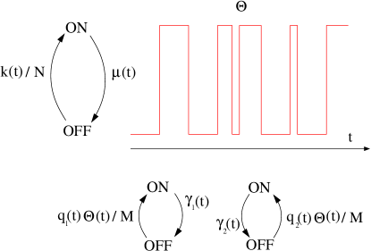
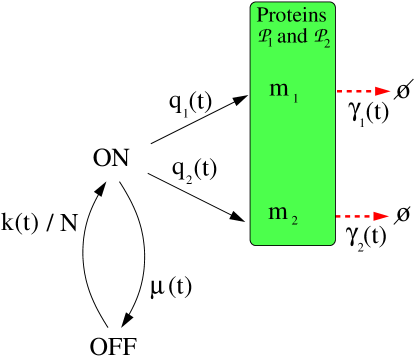
    The PPA-mapping [47] is based on the partitioning of Poisson processes (see Figure (2)). It allows for simplification of the original problem to N𝑁N independent processes all identical to model-1 (see Figure (3) and section (2.4)). In the reduced model, the production of protein is regulated by a biological switch taking values ΞΈ=0πœƒ0\theta=0 (OFF) and ΞΈ=1πœƒ1\theta=1 (ON). Since N𝑁N appears as a parameter of the reduced model, we write GN(1)​(z1,z2,t)subscriptsuperscript𝐺1𝑁subscript𝑧1subscript𝑧2𝑑G^{(1)}_{N}(z_{1},z_{2},t) the generating function of model-1. The latter is related to the original generating function via:

    G(0)​(z1,z2,t)=limNβ†’βˆž[GN(1)​(z1,z2,t)]N.superscript𝐺0subscript𝑧1subscript𝑧2𝑑subscript→𝑁superscriptdelimited-[]subscriptsuperscript𝐺1𝑁subscript𝑧1subscript𝑧2𝑑𝑁\displaystyle G^{(0)}(z_{1},z_{2},t)=\lim_{N\rightarrow\infty}{\Big{[}}G^{(1)}_{N}(z_{1},z_{2},t){\Big{]}}^{N}. (16)
  2. Step 2:

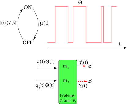
    Denoting by ΘΘ\Theta a particular history (or path) generated by the time evolution of the variable ΞΈπœƒ\theta, we define Ξ¨N​(Θ)subscriptΞ¨π‘Ξ˜\Psi_{N}(\Theta) to be the probability of a given path. Model-2 is defined for one particular history as if frozen (Figure (4)). We write GΘ(2)subscriptsuperscript𝐺2ΘG^{(2)}_{\Theta} as the associated generating function and express GN(1)subscriptsuperscript𝐺1𝑁G^{(1)}_{N} as an average over all possible histories (see section (2.5))

    GN(1)​(z1,z2,t)=βˆ‘Ξ˜Ξ¨N​(Θ)​GΘ(2)​(z1,z2,t).subscriptsuperscript𝐺1𝑁subscript𝑧1subscript𝑧2𝑑subscriptΘsubscriptΞ¨π‘Ξ˜subscriptsuperscript𝐺2Θsubscript𝑧1subscript𝑧2𝑑\displaystyle G^{(1)}_{N}(z_{1},z_{2},t)=\sum_{\Theta}\Psi_{N}(\Theta)G^{(2)}_{\Theta}(z_{1},z_{2},t). (17)

    Once the differential equation for GΘ(2)subscriptsuperscript𝐺2ΘG^{(2)}_{\Theta} has been derived, we will be able to show that protein numbers are uncorrelated in model-2. It follows that GΘ(2)subscriptsuperscript𝐺2ΘG^{(2)}_{\Theta} can be expressed as the product of two functions, each associated to a given protein type:

    GΘ(2)​(z1,z2,t)=∏j=1,2Gj|Θ(2)​(zj,t).subscriptsuperscript𝐺2Θsubscript𝑧1subscript𝑧2𝑑subscriptproduct𝑗12subscriptsuperscript𝐺2conditionalπ‘—Ξ˜subscript𝑧𝑗𝑑\displaystyle G^{(2)}_{\Theta}(z_{1},z_{2},t)=\prod_{j=1,2}G^{(2)}_{j|\Theta}(z_{j},t). (18)
  3. Step 3:

    To access the solution of model-2, we exploit the PPA-mapping one more time. Splitting the creation process into M𝑀M independent processes, it ultimately reduces to the study of biological switches (see model-3 in Figure (5)). Writing GM;j|Θ(3)​(zj,t)subscriptsuperscript𝐺3𝑀conditionalπ‘—Ξ˜subscript𝑧𝑗𝑑G^{(3)}_{M;j|\Theta}(z_{j},t) as the generating function of the switch j𝑗j (j=1,2𝑗12j=1,2), we show the relation (see section (2.6))

Gj|Θ(2)=limMβ†’βˆž[GM;j|Θ(3)]M.subscriptsuperscript𝐺2conditionalπ‘—Ξ˜subscript→𝑀superscriptdelimited-[]subscriptsuperscript𝐺3𝑀conditionalπ‘—Ξ˜π‘€\displaystyle G^{(2)}_{j|\Theta}=\lim_{M\rightarrow\infty}\left[G^{(3)}_{M;j|\Theta}\right]^{M}. (19)

Finally, nesting all steps together, the original generating function is given by

G(0)​(z1,z2,t)=limNβ†’βˆž[βˆ‘Ξ˜Ξ¨N​(Θ)β€‹βˆj=1,2limMβ†’βˆž[GM;j|Θ(3)​(zj,t)]M⏟Gj|Θ(2)​(zj,t)⏟GΘ(2)​(z1,z2,t)⏟GN(1)​(z1,z2,t)]N.superscript𝐺0subscript𝑧1subscript𝑧2𝑑subscript→𝑁superscriptdelimited-[]subscript⏟subscriptΘsubscriptΞ¨π‘Ξ˜subscript⏟subscriptproduct𝑗12subscript⏟subscript→𝑀superscriptdelimited-[]subscriptsuperscript𝐺3𝑀conditionalπ‘—Ξ˜subscript𝑧𝑗𝑑𝑀subscriptsuperscript𝐺2conditionalπ‘—Ξ˜subscript𝑧𝑗𝑑subscriptsuperscript𝐺2Θsubscript𝑧1subscript𝑧2𝑑subscriptsuperscript𝐺1𝑁subscript𝑧1subscript𝑧2𝑑𝑁\displaystyle G^{(0)}(z_{1},z_{2},t)=\lim_{N\rightarrow\infty}{\Bigg{[}}\underbrace{\sum_{\Theta}\Psi_{N}(\Theta)\underbrace{\prod_{j=1,2}\underbrace{\lim_{M\rightarrow\infty}{\Big{[}}G^{(3)}_{M;j|\Theta}(z_{j},t){\Big{]}}^{M}}_{G^{(2)}_{j|\Theta}(z_{j},t)}}_{G^{(2)}_{\Theta}(z_{1},z_{2},t)}}_{G^{(1)}_{N}(z_{1},z_{2},t)}{\Bigg{]}}^{N}. (20)

2.3 Consequences: hierarchy in mean and correlation numbers

Before entering the heart of the subject with the application of the PPA-mapping, one can investigate consequences of these successive transformations. The nesting of generating functions allows us to derive direct relations between mean numbers in the different models. We write ⟨mj⟩N(1)superscriptsubscriptdelimited-⟨⟩subscriptπ‘šπ‘—π‘1\langle m_{j}\rangle_{N}^{(1)}, ⟨mj⟩Θ(2)superscriptsubscriptdelimited-⟨⟩subscriptπ‘šπ‘—Ξ˜2\langle m_{j}\rangle_{\Theta}^{(2)} and ⟨mj⟩M|Θ(3)superscriptsubscriptdelimited-⟨⟩subscriptπ‘šπ‘—conditionalπ‘€Ξ˜3\langle m_{j}\rangle_{M|\Theta}^{(3)} the mean numbers of j𝑗j-proteins in model-1, 2 and 3 respectively. For simplicity, we choose to omit the superscript 00 so that ⟨mj⟩delimited-⟨⟩subscriptπ‘šπ‘—\langle m_{j}\rangle denotes the average number of proteins in the original model. To ease the notations further we choose not to make the time dependance explicit, since the relations derived bellow are true for all time t𝑑t. Equations (16), (17) and (19) bring us to

⟨mj⟩delimited-⟨⟩subscriptπ‘šπ‘—\displaystyle\langle m_{j}\rangle =\displaystyle= limNβ†’βˆžNβ€‹βŸ¨mj⟩N(1),subscript→𝑁𝑁superscriptsubscriptdelimited-⟨⟩subscriptπ‘šπ‘—π‘1\displaystyle\lim_{N\rightarrow\infty}N\langle m_{j}\rangle_{N}^{(1)}, (21)
⟨mj⟩N(1)superscriptsubscriptdelimited-⟨⟩subscriptπ‘šπ‘—π‘1\displaystyle\langle m_{j}\rangle_{N}^{(1)} =\displaystyle= βˆ‘Ξ˜Ξ¨N​(Θ)β€‹βŸ¨mj⟩Θ(2),subscriptΘsubscriptΞ¨π‘Ξ˜subscriptsuperscriptdelimited-⟨⟩subscriptπ‘šπ‘—2Θ\displaystyle\sum_{\Theta}\Psi_{N}(\Theta)\langle m_{j}\rangle^{(2)}_{\Theta}, (22)
⟨mj⟩Θ(2)subscriptsuperscriptdelimited-⟨⟩subscriptπ‘šπ‘—2Θ\displaystyle\langle m_{j}\rangle^{(2)}_{\Theta} =\displaystyle= limMβ†’βˆžMβ€‹βŸ¨mj⟩M|Θ(3).subscript→𝑀𝑀superscriptsubscriptdelimited-⟨⟩subscriptπ‘šπ‘—conditionalπ‘€Ξ˜3\displaystyle\lim_{M\rightarrow\infty}M\langle m_{j}\rangle_{M|\Theta}^{(3)}. (23)

The calculation of ⟨mj⟩(3)superscriptdelimited-⟨⟩subscriptπ‘šπ‘—3\langle m_{j}\rangle^{(3)} is a pretty simple affair. Each protein being reduced to a biological switch, mj(3)superscriptsubscriptπ‘šπ‘—3m_{j}^{(3)} is restricted to the value 00 and 111. We give here, the expression of ⟨mj⟩(3)superscriptdelimited-⟨⟩subscriptπ‘šπ‘—3\langle m_{j}\rangle^{(3)}, for which the derivation is presented in section (2.6):

⟨mj⟩M|Θ(3)=1Mβ€‹βˆ«0tdΞ»β€‹Ξ˜β€‹(Ξ»)​qj​(Ξ»)​eWΞ³j​(Ξ»)βˆ’WΞ³j​(t).superscriptsubscriptdelimited-⟨⟩subscriptπ‘šπ‘—conditionalπ‘€Ξ˜31𝑀superscriptsubscript0𝑑differential-dπœ†Ξ˜πœ†subscriptπ‘žπ‘—πœ†superscript𝑒subscriptπ‘Šsubscriptπ›Ύπ‘—πœ†subscriptπ‘Šsubscript𝛾𝑗𝑑\displaystyle\langle m_{j}\rangle_{M|\Theta}^{(3)}=\frac{1}{M}\int_{0}^{t}\mathrm{d}\lambda\ \Theta(\lambda)q_{j}(\lambda)e^{W_{\gamma_{j}}(\lambda)-W_{\gamma_{j}}(t)}. (24)

To continue further, eq. (22) requires knowledge of the probability Ξ¨N​(Θ)subscriptΞ¨π‘Ξ˜\Psi_{N}(\Theta) for a given path. This is not particularly difficult as one only needs to consider paths with probability up to the order 1/N1𝑁1/N (see section (2.7)). Without further knowledge of the generating function, once Ξ¨N​(Θ)subscriptΞ¨π‘Ξ˜\Psi_{N}(\Theta) and ⟨mj⟩(3)superscriptdelimited-⟨⟩subscriptπ‘šπ‘—3\langle m_{j}\rangle^{(3)} given, the reader can derive the time evolution for mean number of proteins using equations (21), (22) and (23). Practically, those steps give a convoluted way to reach the result already presented in (5). It however reflects on the strategy adopted here to access the generating function.
Considering the correlation function, with the help of Eq. (16), we can show

C1,2=⟨m1​m2βŸ©βˆ’βŸ¨m1βŸ©β€‹βŸ¨m2⟩=limNβ†’βˆžNβ€‹βŸ¨m1​m2⟩N(1).subscript𝐢12delimited-⟨⟩subscriptπ‘š1subscriptπ‘š2delimited-⟨⟩subscriptπ‘š1delimited-⟨⟩subscriptπ‘š2subscript→𝑁𝑁subscriptsuperscriptdelimited-⟨⟩subscriptπ‘š1subscriptπ‘š21𝑁\displaystyle C_{1,2}=\langle m_{1}m_{2}\rangle-\langle m_{1}\rangle\langle m_{2}\rangle=\lim_{N\rightarrow\infty}N\langle m_{1}m_{2}\rangle^{(1)}_{N}. (25)

The protein number being uncorrelated in model-2 we have ⟨m1​m2⟩Θ(2)=⟨m1⟩Θ(2)β€‹βŸ¨m2⟩Θ(2)subscriptsuperscriptdelimited-⟨⟩subscriptπ‘š1subscriptπ‘š22Θsuperscriptsubscriptdelimited-⟨⟩subscriptπ‘š1Θ2superscriptsubscriptdelimited-⟨⟩subscriptπ‘š2Θ2\langle m_{1}m_{2}\rangle^{(2)}_{\Theta}=\langle m_{1}\rangle_{\Theta}^{(2)}\langle m_{2}\rangle_{\Theta}^{(2)}, which leads us to

⟨m1​m2⟩N(1)=βˆ‘Ξ˜Ξ¨N​(Θ)β€‹βŸ¨m1⟩Θ(2)β€‹βŸ¨m2⟩Θ(2).superscriptsubscriptdelimited-⟨⟩subscriptπ‘š1subscriptπ‘š2𝑁1subscriptΘsubscriptΞ¨π‘Ξ˜superscriptsubscriptdelimited-⟨⟩subscriptπ‘š1Θ2superscriptsubscriptdelimited-⟨⟩subscriptπ‘š2Θ2\displaystyle\langle m_{1}m_{2}\rangle_{N}^{(1)}=\sum_{\Theta}\Psi_{N}(\Theta)\langle m_{1}\rangle_{\Theta}^{(2)}\langle m_{2}\rangle_{\Theta}^{(2)}. (26)

From the latter two equations, we conclude that C1,2>0subscript𝐢120C_{1,2}>0 unless at least one of ⟨mj⟩=0delimited-⟨⟩subscriptπ‘šπ‘—0\langle m_{j}\rangle=0 (j=1,2𝑗12j=1,2). Hence, there is no non-trivial point in parameter space such that the correlation between protein number vanishes. As a consequence, there is no region of the parameter space in which the mean field approach is valid. In [49], the authors focus on alternative splicing mechanism, investigating the stationary state of a slightly different model from the one presented here. This study considers the transition from a pre-mRNA to two different mature mRNAs. For constitutive expression (no bursty pre-mRNA creation), they show that (in the stationary state) the mRNA numbers (of type 111 and 222) are independent. They however observe, for bursty pre-mRNA production, the emergence of correlations between the two mature mRNA types.
Refer to caption
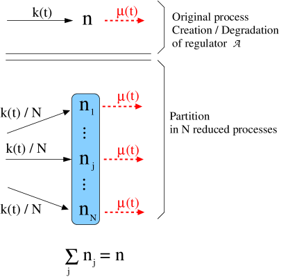
Figure 2: We partition each creation event into N𝑁N ’types’. The creation rate associated to a particular type is given by k​(t)/Nπ‘˜π‘‘π‘k(t)/N. The sum of molecules numbers njsubscript𝑛𝑗n_{j} over each type is equal to the total number of molecules n𝑛n in the original model.

2.4 First transformation: from model-0 to model-1

The PPA-mapping is based on the partitioning property of Poisson processes. Without entering into technical details, the mapping can be understood as follow:

  1. 1.

    Consider the creation/degradation process of regulator π’œπ’œ{\cal A} (with rates k​(t)π‘˜π‘‘k(t) and μ​(t)πœ‡π‘‘\mu(t)).

  2. 2.

    Partition every creation events into N𝑁N ’types’ (Figure (2)). The partition is homogeneous so that each π’œπ’œ{\cal A} molecule is equally likely to be assigned to a given type. It follows that the creation rate associated to a particular type is given by k​(t)/Nπ‘˜π‘‘π‘k(t)/N.

  3. 3.

    Take the limit N≫1much-greater-than𝑁1N\gg 1. As a consequence, the probability of observing more than one π’œπ’œ{\cal A} molecule of a particular type can be neglected. It follows that the random variable describing the number of molecules π’œπ’œ{\cal A} (of a given type) is restricted to the value 00 or 111.

Model-1 as defined under this procedure is illustrated on Figure (3). Note that N𝑁N appears as a parameter in the reduced model. Along the lines presented in [47] we write G(0)=[GN(1)]Nsuperscript𝐺0superscriptdelimited-[]subscriptsuperscript𝐺1𝑁𝑁G^{(0)}=[G^{(1)}_{N}]^{N}. Equation (2.2) shows that GN(1)subscriptsuperscript𝐺1𝑁G^{(1)}_{N} obeys the same differential equation under the transformation k​(t)β†’k​(t)/Nβ†’π‘˜π‘‘π‘˜π‘‘π‘k(t)\rightarrow k(t)/N. As a consequence the probability of observing (in the reduced model) more than one π’œπ’œ{\cal A} molecule is of order 1/N21superscript𝑁21/N^{2} and can be neglected as Nβ†’βˆžβ†’π‘N\rightarrow\infty. While the previous logical argument shows how model-1 is emerging from model-0, an alternative derivation, based on the probability distribution instead of the generating function, allows for the reversed construction: building model-0 starting with N𝑁N independent model-1. This derivation, not presented in the literature so far, is presented in an appendix.
Refer to caption
Figure 3: Model-1: The creation and degradation of two types of proteins (𝒫1subscript𝒫1{\cal P}_{1} and 𝒫2subscript𝒫2{\cal P}_{2}) is regulated by an upstream switch. Transition rates for proteins production and degradation are respectively written qj​(t)subscriptπ‘žπ‘—π‘‘q_{j}(t) and Ξ³j​(t)subscript𝛾𝑗𝑑\gamma_{j}(t) (with j=1,2𝑗12j=1,2), while k​(t)/Nπ‘˜π‘‘π‘k(t)/N and μ​(t)πœ‡π‘‘\mu(t) denote the probabilities of transition from O​F​Fβ†’O​N→𝑂𝐹𝐹𝑂𝑁OFF\rightarrow ON and O​Nβ†’O​F​F→𝑂𝑁𝑂𝐹𝐹ON\rightarrow OFF.

2.5 Second transformation: from model-1 to model-2

Let us remind the reader that ΞΈπœƒ\theta is the new stochastic variable (taking value in {0,1}01\{0,1\}) emerging in model-1. The decomposition over all possible histories, generated by the variable ΞΈπœƒ\theta, emerges from the use of conditional probabilities. To be more explicit we write ΘΘ\Theta as a particular history associated to the variable ΞΈπœƒ\theta. For a given path, we write Ξ˜β€‹(t)Ξ˜π‘‘\Theta(t) as the value taken by the random variable ΞΈπœƒ\theta at time t𝑑t. We continue further by writing Ο†N;(Θ,a,b)​(t)subscriptπœ‘π‘Ξ˜π‘Žπ‘π‘‘\varphi_{N;(\Theta,a,b)}(t) as the probability associated to a particular history ΘΘ\Theta and protein numbers aπ‘Ža and b𝑏b. The generating function GN(1)subscriptsuperscript𝐺1𝑁G^{(1)}_{N} can be rewritten as

GN(1)​(z1,z2,t)=βˆ‘Ξ˜,a,bz1a​z2b​φN;(Θ,a,b)​(t).subscriptsuperscript𝐺1𝑁subscript𝑧1subscript𝑧2𝑑subscriptΞ˜π‘Žπ‘superscriptsubscript𝑧1π‘Žsuperscriptsubscript𝑧2𝑏subscriptπœ‘π‘Ξ˜π‘Žπ‘π‘‘\displaystyle G^{(1)}_{N}(z_{1},z_{2},t)=\sum_{\Theta,a,b}z_{1}^{a}z_{2}^{b}\varphi_{N;(\Theta,a,b)}(t). (27)

Defining ψa,b|Ξ˜β€‹(t)subscriptπœ“π‘Žconditionalπ‘Ξ˜π‘‘\psi_{a,b|\Theta}(t) as the conditional probability on ΘΘ\Theta while Ξ¨N​(Θ)subscriptΞ¨π‘Ξ˜\Psi_{N}(\Theta) is the probability of a given history, the equality Ο†N;(Θ,a,b)​(t)=Ξ¨N​(Θ)β€‹Οˆa,b|Ξ˜β€‹(t)subscriptπœ‘π‘Ξ˜π‘Žπ‘π‘‘subscriptΞ¨π‘Ξ˜subscriptπœ“π‘Žconditionalπ‘Ξ˜π‘‘\varphi_{N;(\Theta,a,b)}(t)=\Psi_{N}(\Theta)\psi_{a,b|\Theta}(t) leads to

GN(1)​(z1,z2,t)=βˆ‘Ξ˜Ξ¨N​(Θ)​GΘ(2)​(z1,z2,t),subscriptsuperscript𝐺1𝑁subscript𝑧1subscript𝑧2𝑑subscriptΘsubscriptΞ¨π‘Ξ˜subscriptsuperscript𝐺2Θsubscript𝑧1subscript𝑧2𝑑\displaystyle G^{(1)}_{N}(z_{1},z_{2},t)=\sum_{\Theta}\Psi_{N}(\Theta)G^{(2)}_{\Theta}(z_{1},z_{2},t), (28)

with

GΘ(2)​(z1,z2,t)=βˆ‘a,bz1a​z2bβ€‹Οˆa,b|Ξ˜β€‹(t).subscriptsuperscript𝐺2Θsubscript𝑧1subscript𝑧2𝑑subscriptπ‘Žπ‘superscriptsubscript𝑧1π‘Žsuperscriptsubscript𝑧2𝑏subscriptπœ“π‘Žconditionalπ‘Ξ˜π‘‘\displaystyle G^{(2)}_{\Theta}(z_{1},z_{2},t)=\sum_{a,b}z_{1}^{a}z_{2}^{b}\psi_{a,b|\Theta}(t). (29)

For a known history Ξ˜β€‹(t)Ξ˜π‘‘\Theta(t), we have

d​GΘ(2)d​t𝑑subscriptsuperscript𝐺2Ξ˜π‘‘π‘‘\displaystyle\frac{dG^{(2)}_{\Theta}}{dt} =\displaystyle= (z1βˆ’1)​(q1​(t)β€‹Ξ˜β€‹(t)βˆ’Ξ³1​(t)β€‹βˆ‚z1)​GΘ(2)subscript𝑧11subscriptπ‘ž1π‘‘Ξ˜π‘‘subscript𝛾1𝑑subscriptsubscript𝑧1subscriptsuperscript𝐺2Θ\displaystyle(z_{1}-1)(q_{1}(t)\Theta(t)-\gamma_{1}(t)\partial_{z_{1}})G^{(2)}_{\Theta}
+\displaystyle+ (z2βˆ’1)​(q2​(t)β€‹Ξ˜β€‹(t)βˆ’Ξ³2​(t)β€‹βˆ‚z2)​GΘ(2).subscript𝑧21subscriptπ‘ž2π‘‘Ξ˜π‘‘subscript𝛾2𝑑subscriptsubscript𝑧2subscriptsuperscript𝐺2Θ\displaystyle(z_{2}-1)(q_{2}(t)\Theta(t)-\gamma_{2}(t)\partial_{z_{2}})G^{(2)}_{\Theta}.

Note that in the last equation GΘ(2)subscriptsuperscript𝐺2ΘG^{(2)}_{\Theta} is clearly independent of N𝑁N and so is the conditional probability ψa,b|Θsubscriptπœ“π‘Žconditionalπ‘Ξ˜\psi_{a,b|\Theta}. The dependence in N𝑁N is now carried by the probability Ξ¨NsubscriptΨ𝑁\Psi_{N}. At this point we see that GΘ(2)subscriptsuperscript𝐺2ΘG^{(2)}_{\Theta} can be written as

GΘ(2)​(z1,z2,t)=∏j=1,2Gj|Θ(2)​(zj,t),subscriptsuperscript𝐺2Θsubscript𝑧1subscript𝑧2𝑑subscriptproduct𝑗12subscriptsuperscript𝐺2conditionalπ‘—Ξ˜subscript𝑧𝑗𝑑\displaystyle G^{(2)}_{\Theta}(z_{1},z_{2},t)=\prod_{j=1,2}G^{(2)}_{j|\Theta}(z_{j},t), (31)

where each generating function is governed by

d​Gj|Θ(2)d​t=(zjβˆ’1)​(qj​(t)β€‹Ξ˜β€‹(t)βˆ’Ξ³j​(t)β€‹βˆ‚zj)​Gj|Θ(2).𝑑subscriptsuperscript𝐺2conditionalπ‘—Ξ˜π‘‘π‘‘subscript𝑧𝑗1subscriptπ‘žπ‘—π‘‘Ξ˜π‘‘subscript𝛾𝑗𝑑subscriptsubscript𝑧𝑗subscriptsuperscript𝐺2conditionalπ‘—Ξ˜\displaystyle\frac{dG^{(2)}_{j|\Theta}}{dt}=(z_{j}-1)(q_{j}(t)\Theta(t)-\gamma_{j}(t)\partial_{z_{j}})G^{(2)}_{j|\Theta}. (32)

Thereupon the two protein numbers are uncorrelated in model-2.
Refer to caption
Figure 4: Model-2: The creation and degradation of two types of proteins (𝒫1subscript𝒫1{\cal P}_{1} and 𝒫2subscript𝒫2{\cal P}_{2}) for a fixed history ΘΘ\Theta. Transition rates for proteins production and degradation are respectively written qj​(t)β€‹Ξ˜β€‹(t)subscriptπ‘žπ‘—π‘‘Ξ˜π‘‘q_{j}(t)\Theta(t) and Ξ³j​(t)subscript𝛾𝑗𝑑\gamma_{j}(t) (with j=1,2𝑗12j=1,2).

2.6 Third transformation: from model-2 to model-3

To reach the expression of GΘ(2)subscriptsuperscript𝐺2ΘG^{(2)}_{\Theta}, one applies the PPA-mapping one more time. This will reduce the original model to the study of biological switches (Figure (5)). For each protein type 𝒫jsubscript𝒫𝑗{\cal P}_{j} (j=1,2𝑗12j=1,2), we once again, choose to partition every creation event into M𝑀M groups. The partition being homogeneous, each protein is equally likely to be assigned to a given group. The creation rate for a particular group is given by qj​(t)/Msubscriptπ‘žπ‘—π‘‘π‘€q_{j}(t)/M. Taking the limit M≫1much-greater-than𝑀1M\gg 1 allows us to neglect the creation of more than one protein in each group. To be explicit one writes Gj|Θ(2)=[GM;j|Θ(3)]Msubscriptsuperscript𝐺2conditionalπ‘—Ξ˜superscriptdelimited-[]subscriptsuperscript𝐺3𝑀conditionalπ‘—Ξ˜π‘€G^{(2)}_{j|\Theta}=[G^{(3)}_{M;j|\Theta}]^{M} in equation (32). This procedure leads to the same differential equation with the transformation qj​(t)β€‹Ξ˜β€‹(t)β†’qj​(t)β€‹Ξ˜β€‹(t)/Mβ†’subscriptπ‘žπ‘—π‘‘Ξ˜π‘‘subscriptπ‘žπ‘—π‘‘Ξ˜π‘‘π‘€q_{j}(t)\Theta(t)\rightarrow q_{j}(t)\Theta(t)/M. Hence, in the limit Mβ†’βˆžβ†’π‘€M\rightarrow\infty, the number of proteins of type j𝑗j are restricted to 00 and 111. It follows that

GΘ(2)=∏j=1,2limMβ†’βˆž[GM;j|Θ(3)]M.subscriptsuperscript𝐺2Θsubscriptproduct𝑗12subscript→𝑀superscriptdelimited-[]subscriptsuperscript𝐺3𝑀conditionalπ‘—Ξ˜π‘€\displaystyle G^{(2)}_{\Theta}=\prod_{j=1,2}\lim_{M\rightarrow\infty}{\Big{[}}G^{(3)}_{M;j|\Theta}{\Big{]}}^{M}. (33)

The function GM;j|Θ(3)subscriptsuperscript𝐺3𝑀conditionalπ‘—Ξ˜G^{(3)}_{M;j|\Theta} describes the dynamics of a two-state model and can be written has

GM;j|Θ(3)​(z,t)=1+(zβˆ’1)​fM;j|Θ,subscriptsuperscript𝐺3𝑀conditionalπ‘—Ξ˜π‘§π‘‘1𝑧1subscript𝑓𝑀conditionalπ‘—Ξ˜\displaystyle G^{(3)}_{M;j|\Theta}(z,t)=1+(z-1)f_{M;j|\Theta}, (34)

where fM;j|Θsubscript𝑓𝑀conditionalπ‘—Ξ˜f_{M;j|\Theta} is the probability to find the switch j𝑗j in the ON-state, knowing the history ΘΘ\Theta. The latter is the solution of the following equation

d​fM;j|Θd​t=qj​(t)β€‹Ξ˜β€‹(t)/Mβˆ’[Ξ³j​(t)+qj​(t)β€‹Ξ˜β€‹(t)/M]​fM;j|Θ.𝑑subscript𝑓𝑀conditionalπ‘—Ξ˜π‘‘π‘‘subscriptπ‘žπ‘—π‘‘Ξ˜π‘‘π‘€delimited-[]subscript𝛾𝑗𝑑subscriptπ‘žπ‘—π‘‘Ξ˜π‘‘π‘€subscript𝑓𝑀conditionalπ‘—Ξ˜\displaystyle\frac{df_{M;j|\Theta}}{dt}=q_{j}(t)\Theta(t)/M-\left[\gamma_{j}(t)+q_{j}(t)\Theta(t)/M\right]f_{M;j|\Theta}. (35)

We now have reached the point where one needs to define the initial state. We choose to consider fM;j|Ξ˜β€‹(t=0)=0subscript𝑓𝑀conditionalπ‘—Ξ˜π‘‘00f_{M;j|\Theta}(t=0)=0. Let us remind the reader that, in model-3, the total number of switches j𝑗j in the ON-state equals the number of proteins 𝒫jsubscript𝒫𝑗{\cal P}_{j} in model-2. The hierarchy builds up to the number of proteins in model-0. As we look at equation (21), (22) and (23), we see that choosing (at time t=0𝑑0t=0) all switches (j=1,2𝑗12j=1,2) in the OFF-state, imposes the following initial state on to the original model

m1​(t=0)=m2​(t=0)=0.subscriptπ‘š1𝑑0subscriptπ‘š2𝑑00\displaystyle m_{1}(t=0)=m_{2}(t=0)=0. (36)

A simple calculation gives

fM;j|Ξ˜β€‹(t)=∫0tdλ​qj​(Ξ»)Mβ€‹Ξ˜β€‹(Ξ»)​exp⁑[βˆ’βˆ«Ξ»tds​{Ξ³j​(s)+qj​(s)Mβ€‹Ξ˜β€‹(s)}],subscript𝑓𝑀conditionalπ‘—Ξ˜π‘‘superscriptsubscript0𝑑differential-dπœ†subscriptπ‘žπ‘—πœ†π‘€Ξ˜πœ†superscriptsubscriptπœ†π‘‘differential-d𝑠subscript𝛾𝑗𝑠subscriptπ‘žπ‘—π‘ π‘€Ξ˜π‘ \displaystyle f_{M;j|\Theta}(t)=\int_{0}^{t}\mathrm{d}\lambda\ \frac{q_{j}(\lambda)}{M}\Theta(\lambda)\exp\left[-\int_{\lambda}^{t}\mathrm{d}s\ \left\{\gamma_{j}(s)+\frac{q_{j}(s)}{M}\Theta(s)\right\}\right], (37)

which, to the first order in 1/M1𝑀1/M, simplifies to

fM;j|Ξ˜β€‹(t)subscript𝑓𝑀conditionalπ‘—Ξ˜π‘‘\displaystyle f_{M;j|\Theta}(t) =\displaystyle= Ξ›j|Ξ˜β€‹(t)/M,subscriptΞ›conditionalπ‘—Ξ˜π‘‘π‘€\displaystyle{\Lambda_{j|\Theta}(t)}/{M}, (38)

with

Ξ›j|Ξ˜β€‹(t)=∫0tdΞ»β€‹Ξ˜β€‹(Ξ»)​qj​(Ξ»)​eWΞ³j​(Ξ»)βˆ’WΞ³j​(t).subscriptΞ›conditionalπ‘—Ξ˜π‘‘superscriptsubscript0𝑑differential-dπœ†Ξ˜πœ†subscriptπ‘žπ‘—πœ†superscript𝑒subscriptπ‘Šsubscriptπ›Ύπ‘—πœ†subscriptπ‘Šsubscript𝛾𝑗𝑑\displaystyle\Lambda_{j|\Theta}(t)=\int_{0}^{t}\mathrm{d}\lambda\ \Theta(\lambda)q_{j}(\lambda)e^{W_{\gamma_{j}}(\lambda)-W_{\gamma_{j}}(t)}. (39)

Nesting equation (38) into (34) leads to:

GM;j|Θ(3)​(z,t)=1+(zβˆ’1)​Λj|Ξ˜β€‹(t)/M.subscriptsuperscript𝐺3𝑀conditionalπ‘—Ξ˜π‘§π‘‘1𝑧1subscriptΞ›conditionalπ‘—Ξ˜π‘‘π‘€\displaystyle G^{(3)}_{M;j|\Theta}(z,t)=1+(z-1){\Lambda_{j|\Theta}(t)}/{M}. (40)

With Eq. (33) the latter result allows us to write

GΘ(2)​(z1,z2,t)=exp⁑[βˆ‘j=1,2(zjβˆ’1)​Λj|Ξ˜β€‹(t)].subscriptsuperscript𝐺2Θsubscript𝑧1subscript𝑧2𝑑subscript𝑗12subscript𝑧𝑗1subscriptΞ›conditionalπ‘—Ξ˜π‘‘\displaystyle G^{(2)}_{\Theta}(z_{1},z_{2},t)=\exp\left[\sum_{j=1,2}(z_{j}-1)\Lambda_{j|\Theta}(t)\right]. (41)
Refer to caption
Figure 5: Model-3 describes, for a fixed history ΘΘ\Theta, two biological switches for which transition rates are respectively written qj​(t)β€‹Ξ˜β€‹(t)/Msubscriptπ‘žπ‘—π‘‘Ξ˜π‘‘π‘€q_{j}(t)\Theta(t)/M and Ξ³j​(t)subscript𝛾𝑗𝑑\gamma_{j}(t) (with j=1,2𝑗12j=1,2).

2.7 Summing over all histories

In order to derive the generating function GN(1)subscriptsuperscript𝐺1𝑁G^{(1)}_{N} from GΘ(2)subscriptsuperscript𝐺2ΘG^{(2)}_{\Theta}, using equation (17), we focus on the expression of the probability Ξ¨N​(Θ)subscriptΞ¨π‘Ξ˜\Psi_{N}(\Theta) for all relevant histories ΘΘ\Theta. As mentioned earlier, we simply need to evaluate Ξ¨N​(Θ)subscriptΞ¨π‘Ξ˜\Psi_{N}(\Theta) up to the order 1/N1𝑁1/N. We choose to consider the initial state Ξ˜β€‹(t=0)=0Ξ˜π‘‘00\Theta(t=0)=0. Amongst N𝑁N identical models, the number of switches in the ON-states defines the number n𝑛n of molecules π’œπ’œ{\cal A}. It follows that the initial state must satisfy:

n​(t=0)=0.𝑛𝑑00\displaystyle n(t=0)=0. (42)

Together, equations (36) and (42) fully specify the initial state, so that P0,0,0​(t=0)=1subscript𝑃000𝑑01P_{0,0,0}(t=0)=1. We remind the reader that the probability of the transition form O​Nβ†’O​F​F→𝑂𝑁𝑂𝐹𝐹ON\rightarrow OFF (between time t𝑑t and t+δ​t𝑑𝛿𝑑t+\delta t) is given by μ​(t)​δ​tπœ‡π‘‘π›Ώπ‘‘\mu(t)\delta t. In addition, the probability of observing the transition O​F​Fβ†’O​N→𝑂𝐹𝐹𝑂𝑁OFF\rightarrow ON is given by k​(t)​δ​t/Nπ‘˜π‘‘π›Ώπ‘‘π‘k(t)\delta t/N. At the first order in 1/N1𝑁1/N, three different types of histories are relevant. They are symbolically represented by , and and detailed in table (2). The probability associated to each path is

Ξ¨N​(Β Β )≃1βˆ’1Nβ€‹βˆ«0tds​k​(s),similar-to-or-equalssubscriptΨ𝑁  11𝑁superscriptsubscript0𝑑differential-dπ‘ π‘˜π‘ \displaystyle\Psi_{N}\left({\makebox[13.0pt][l]{ \leavevmode\hbox to11.16pt{\vbox to0.4pt{\pgfpicture\makeatletter\hbox{\hskip 0.2pt\lower-0.2pt\hbox to0.0pt{\pgfsys@beginscope\pgfsys@invoke{ }\definecolor{pgfstrokecolor}{rgb}{0,0,0}\pgfsys@color@rgb@stroke{0}{0}{0}\pgfsys@invoke{ }\pgfsys@color@rgb@fill{0}{0}{0}\pgfsys@invoke{ }\pgfsys@setlinewidth{0.4pt}\pgfsys@invoke{ }\nullfont\hbox to0.0pt{\pgfsys@beginscope\pgfsys@invoke{ }{{}}{{}{}}{{}}{} {}{}{}{}{}{}{{}}\pgfsys@moveto{0.0pt}{0.0pt}\pgfsys@lineto{10.30386pt}{0.0pt}\pgfsys@stroke\pgfsys@invoke{ }{{}{{}}{}{}{{}}{{{}}{{{}}{\pgfsys@beginscope\pgfsys@invoke{ }\pgfsys@transformcm{1.0}{0.0}{0.0}{1.0}{10.30386pt}{0.0pt}\pgfsys@invoke{ }\pgfsys@invoke{ \lxSVG@closescope }\pgfsys@invoke{\lxSVG@closescope }\pgfsys@endscope}}{{}}}} \pgfsys@invoke{\lxSVG@closescope }\pgfsys@endscope{}{}{}\hss}\pgfsys@discardpath\pgfsys@invoke{\lxSVG@closescope }\pgfsys@endscope\hss}}\lxSVG@closescope\endpgfpicture}} }}\right)\simeq 1-\frac{1}{N}\int_{0}^{t}\mathrm{d}s\ k(s), (43)
Ξ¨N​(Β Β )≃k​(s)N​eWμ​(s)βˆ’Wμ​(t),similar-to-or-equalssubscriptΞ¨π‘Β Β π‘˜π‘ π‘superscript𝑒subscriptπ‘Šπœ‡π‘ subscriptπ‘Šπœ‡π‘‘\displaystyle\Psi_{N}\left({\makebox[13.0pt][l]{ \leavevmode\hbox to11.16pt{\vbox to5.78pt{\pgfpicture\makeatletter\hbox{\hskip 0.2pt\lower-0.2pt\hbox to0.0pt{\pgfsys@beginscope\pgfsys@invoke{ }\definecolor{pgfstrokecolor}{rgb}{0,0,0}\pgfsys@color@rgb@stroke{0}{0}{0}\pgfsys@invoke{ }\pgfsys@color@rgb@fill{0}{0}{0}\pgfsys@invoke{ }\pgfsys@setlinewidth{0.4pt}\pgfsys@invoke{ }\nullfont\hbox to0.0pt{\pgfsys@beginscope\pgfsys@invoke{ }{{}}{}{{}}{} {}{}{}\pgfsys@moveto{0.0pt}{0.0pt}\pgfsys@lineto{5.38193pt}{0.0pt}\pgfsys@stroke\pgfsys@invoke{ } {}{{}}{} {}{}{}\pgfsys@moveto{5.38193pt}{0.0pt}\pgfsys@lineto{5.38193pt}{5.38193pt}\pgfsys@stroke\pgfsys@invoke{ } {}{{}}{} {}{}{}{}{}{}{{}}\pgfsys@moveto{5.38193pt}{5.38193pt}\pgfsys@lineto{10.30386pt}{5.38193pt}\pgfsys@stroke\pgfsys@invoke{ }{{}{{}}{}{}{{}}{{{}}{{{}}{\pgfsys@beginscope\pgfsys@invoke{ }\pgfsys@transformcm{1.0}{0.0}{0.0}{1.0}{10.30386pt}{5.38193pt}\pgfsys@invoke{ }\pgfsys@invoke{ \lxSVG@closescope }\pgfsys@invoke{\lxSVG@closescope }\pgfsys@endscope}}{{}}}} \pgfsys@invoke{\lxSVG@closescope }\pgfsys@endscope{}{}{}\hss}\pgfsys@discardpath\pgfsys@invoke{\lxSVG@closescope }\pgfsys@endscope\hss}}\lxSVG@closescope\endpgfpicture}} }}\right)\simeq\frac{k(s)}{N}e^{W_{\mu}(s)-W_{\mu}(t)}, (44)
Ξ¨N​(Β Β )≃k​(s)N​μ​(sβ€²)​eWμ​(s)βˆ’Wμ​(sβ€²).similar-to-or-equalssubscriptΞ¨π‘Β Β π‘˜π‘ π‘πœ‡superscript𝑠′superscript𝑒subscriptπ‘Šπœ‡π‘ subscriptπ‘Šπœ‡superscript𝑠′\displaystyle\Psi_{N}\left({\makebox[20.0pt][l]{ \leavevmode\hbox to16.55pt{\vbox to5.78pt{\pgfpicture\makeatletter\hbox{\hskip 0.2pt\lower-0.2pt\hbox to0.0pt{\pgfsys@beginscope\pgfsys@invoke{ }\definecolor{pgfstrokecolor}{rgb}{0,0,0}\pgfsys@color@rgb@stroke{0}{0}{0}\pgfsys@invoke{ }\pgfsys@color@rgb@fill{0}{0}{0}\pgfsys@invoke{ }\pgfsys@setlinewidth{0.4pt}\pgfsys@invoke{ }\nullfont\hbox to0.0pt{\pgfsys@beginscope\pgfsys@invoke{ }{{}}{}{{}}{} {}{}{}\pgfsys@moveto{0.0pt}{0.0pt}\pgfsys@lineto{5.38193pt}{0.0pt}\pgfsys@stroke\pgfsys@invoke{ } {}{{}}{} {}{}{}\pgfsys@moveto{5.38193pt}{0.0pt}\pgfsys@lineto{5.38193pt}{5.38193pt}\pgfsys@stroke\pgfsys@invoke{ } {}{{}}{} {}{}{}\pgfsys@moveto{5.38193pt}{5.38193pt}\pgfsys@lineto{10.76385pt}{5.38193pt}\pgfsys@stroke\pgfsys@invoke{ } {}{{}}{} {}{}{}\pgfsys@moveto{10.76385pt}{5.38193pt}\pgfsys@lineto{10.76385pt}{0.0pt}\pgfsys@stroke\pgfsys@invoke{ } {}{{}}{} {}{}{}{}{}{}{{}}\pgfsys@moveto{10.76385pt}{0.0pt}\pgfsys@lineto{15.68579pt}{0.0pt}\pgfsys@stroke\pgfsys@invoke{ }{{}{{}}{}{}{{}}{{{}}{{{}}{\pgfsys@beginscope\pgfsys@invoke{ }\pgfsys@transformcm{1.0}{0.0}{0.0}{1.0}{15.68579pt}{0.0pt}\pgfsys@invoke{ }\pgfsys@invoke{ \lxSVG@closescope }\pgfsys@invoke{\lxSVG@closescope }\pgfsys@endscope}}{{}}}} \pgfsys@invoke{\lxSVG@closescope }\pgfsys@endscope{}{}{}\hss}\pgfsys@discardpath\pgfsys@invoke{\lxSVG@closescope }\pgfsys@endscope\hss}}\lxSVG@closescope\endpgfpicture}} }}\right)\simeq\frac{k(s)}{N}\mu(s^{\prime})e^{W_{\mu}(s)-W_{\mu}(s^{\prime})}. (45)

It is particularly useful to rewrite the last equation as

Ξ¨N​(Β Β )β‰ƒβˆ’k​(s)N​eWμ​(s)​(βˆ‚sβ€²eβˆ’Wμ​(sβ€²)),similar-to-or-equalssubscriptΞ¨π‘Β Β π‘˜π‘ π‘superscript𝑒subscriptπ‘Šπœ‡π‘ subscriptsuperscript𝑠′superscript𝑒subscriptπ‘Šπœ‡superscript𝑠′\displaystyle\Psi_{N}\left({\makebox[20.0pt][l]{ \leavevmode\hbox to16.55pt{\vbox to5.78pt{\pgfpicture\makeatletter\hbox{\hskip 0.2pt\lower-0.2pt\hbox to0.0pt{\pgfsys@beginscope\pgfsys@invoke{ }\definecolor{pgfstrokecolor}{rgb}{0,0,0}\pgfsys@color@rgb@stroke{0}{0}{0}\pgfsys@invoke{ }\pgfsys@color@rgb@fill{0}{0}{0}\pgfsys@invoke{ }\pgfsys@setlinewidth{0.4pt}\pgfsys@invoke{ }\nullfont\hbox to0.0pt{\pgfsys@beginscope\pgfsys@invoke{ }{{}}{}{{}}{} {}{}{}\pgfsys@moveto{0.0pt}{0.0pt}\pgfsys@lineto{5.38193pt}{0.0pt}\pgfsys@stroke\pgfsys@invoke{ } {}{{}}{} {}{}{}\pgfsys@moveto{5.38193pt}{0.0pt}\pgfsys@lineto{5.38193pt}{5.38193pt}\pgfsys@stroke\pgfsys@invoke{ } {}{{}}{} {}{}{}\pgfsys@moveto{5.38193pt}{5.38193pt}\pgfsys@lineto{10.76385pt}{5.38193pt}\pgfsys@stroke\pgfsys@invoke{ } {}{{}}{} {}{}{}\pgfsys@moveto{10.76385pt}{5.38193pt}\pgfsys@lineto{10.76385pt}{0.0pt}\pgfsys@stroke\pgfsys@invoke{ } {}{{}}{} {}{}{}{}{}{}{{}}\pgfsys@moveto{10.76385pt}{0.0pt}\pgfsys@lineto{15.68579pt}{0.0pt}\pgfsys@stroke\pgfsys@invoke{ }{{}{{}}{}{}{{}}{{{}}{{{}}{\pgfsys@beginscope\pgfsys@invoke{ }\pgfsys@transformcm{1.0}{0.0}{0.0}{1.0}{15.68579pt}{0.0pt}\pgfsys@invoke{ }\pgfsys@invoke{ \lxSVG@closescope }\pgfsys@invoke{\lxSVG@closescope }\pgfsys@endscope}}{{}}}} \pgfsys@invoke{\lxSVG@closescope }\pgfsys@endscope{}{}{}\hss}\pgfsys@discardpath\pgfsys@invoke{\lxSVG@closescope }\pgfsys@endscope\hss}}\lxSVG@closescope\endpgfpicture}} }}\right)\simeq-\frac{k(s)}{N}e^{W_{\mu}(s)}\left(\partial_{s^{\prime}}e^{-W_{\mu}(s^{\prime})}\right), (46)

which can be used to verify the conservation of probability:

Ξ¨N​(Β Β )+∫0tds​ΨN​(Β Β )+∫0tdsβ€‹βˆ«stds′​ΨN​(Β Β )=1.subscriptΨ𝑁  superscriptsubscript0𝑑differential-d𝑠subscriptΨ𝑁  superscriptsubscript0𝑑differential-d𝑠superscriptsubscript𝑠𝑑differential-dsuperscript𝑠′subscriptΨ𝑁  1\displaystyle\Psi_{N}\left({\makebox[13.0pt][l]{ \leavevmode\hbox to11.16pt{\vbox to0.4pt{\pgfpicture\makeatletter\hbox{\hskip 0.2pt\lower-0.2pt\hbox to0.0pt{\pgfsys@beginscope\pgfsys@invoke{ }\definecolor{pgfstrokecolor}{rgb}{0,0,0}\pgfsys@color@rgb@stroke{0}{0}{0}\pgfsys@invoke{ }\pgfsys@color@rgb@fill{0}{0}{0}\pgfsys@invoke{ }\pgfsys@setlinewidth{0.4pt}\pgfsys@invoke{ }\nullfont\hbox to0.0pt{\pgfsys@beginscope\pgfsys@invoke{ }{{}}{{}{}}{{}}{} {}{}{}{}{}{}{{}}\pgfsys@moveto{0.0pt}{0.0pt}\pgfsys@lineto{10.30386pt}{0.0pt}\pgfsys@stroke\pgfsys@invoke{ }{{}{{}}{}{}{{}}{{{}}{{{}}{\pgfsys@beginscope\pgfsys@invoke{ }\pgfsys@transformcm{1.0}{0.0}{0.0}{1.0}{10.30386pt}{0.0pt}\pgfsys@invoke{ }\pgfsys@invoke{ \lxSVG@closescope }\pgfsys@invoke{\lxSVG@closescope }\pgfsys@endscope}}{{}}}} \pgfsys@invoke{\lxSVG@closescope }\pgfsys@endscope{}{}{}\hss}\pgfsys@discardpath\pgfsys@invoke{\lxSVG@closescope }\pgfsys@endscope\hss}}\lxSVG@closescope\endpgfpicture}} }}\right)+\int_{0}^{t}\mathrm{d}s\ \hphantom{.}\Psi_{N}\left({\makebox[13.0pt][l]{ \leavevmode\hbox to11.16pt{\vbox to5.78pt{\pgfpicture\makeatletter\hbox{\hskip 0.2pt\lower-0.2pt\hbox to0.0pt{\pgfsys@beginscope\pgfsys@invoke{ }\definecolor{pgfstrokecolor}{rgb}{0,0,0}\pgfsys@color@rgb@stroke{0}{0}{0}\pgfsys@invoke{ }\pgfsys@color@rgb@fill{0}{0}{0}\pgfsys@invoke{ }\pgfsys@setlinewidth{0.4pt}\pgfsys@invoke{ }\nullfont\hbox to0.0pt{\pgfsys@beginscope\pgfsys@invoke{ }{{}}{}{{}}{} {}{}{}\pgfsys@moveto{0.0pt}{0.0pt}\pgfsys@lineto{5.38193pt}{0.0pt}\pgfsys@stroke\pgfsys@invoke{ } {}{{}}{} {}{}{}\pgfsys@moveto{5.38193pt}{0.0pt}\pgfsys@lineto{5.38193pt}{5.38193pt}\pgfsys@stroke\pgfsys@invoke{ } {}{{}}{} {}{}{}{}{}{}{{}}\pgfsys@moveto{5.38193pt}{5.38193pt}\pgfsys@lineto{10.30386pt}{5.38193pt}\pgfsys@stroke\pgfsys@invoke{ }{{}{{}}{}{}{{}}{{{}}{{{}}{\pgfsys@beginscope\pgfsys@invoke{ }\pgfsys@transformcm{1.0}{0.0}{0.0}{1.0}{10.30386pt}{5.38193pt}\pgfsys@invoke{ }\pgfsys@invoke{ \lxSVG@closescope }\pgfsys@invoke{\lxSVG@closescope }\pgfsys@endscope}}{{}}}} \pgfsys@invoke{\lxSVG@closescope }\pgfsys@endscope{}{}{}\hss}\pgfsys@discardpath\pgfsys@invoke{\lxSVG@closescope }\pgfsys@endscope\hss}}\lxSVG@closescope\endpgfpicture}} }}\right)+\int_{0}^{t}\mathrm{d}s\int_{s}^{t}\mathrm{d}s^{\prime}\ \Psi_{N}\left({\makebox[20.0pt][l]{ \leavevmode\hbox to16.55pt{\vbox to5.78pt{\pgfpicture\makeatletter\hbox{\hskip 0.2pt\lower-0.2pt\hbox to0.0pt{\pgfsys@beginscope\pgfsys@invoke{ }\definecolor{pgfstrokecolor}{rgb}{0,0,0}\pgfsys@color@rgb@stroke{0}{0}{0}\pgfsys@invoke{ }\pgfsys@color@rgb@fill{0}{0}{0}\pgfsys@invoke{ }\pgfsys@setlinewidth{0.4pt}\pgfsys@invoke{ }\nullfont\hbox to0.0pt{\pgfsys@beginscope\pgfsys@invoke{ }{{}}{}{{}}{} {}{}{}\pgfsys@moveto{0.0pt}{0.0pt}\pgfsys@lineto{5.38193pt}{0.0pt}\pgfsys@stroke\pgfsys@invoke{ } {}{{}}{} {}{}{}\pgfsys@moveto{5.38193pt}{0.0pt}\pgfsys@lineto{5.38193pt}{5.38193pt}\pgfsys@stroke\pgfsys@invoke{ } {}{{}}{} {}{}{}\pgfsys@moveto{5.38193pt}{5.38193pt}\pgfsys@lineto{10.76385pt}{5.38193pt}\pgfsys@stroke\pgfsys@invoke{ } {}{{}}{} {}{}{}\pgfsys@moveto{10.76385pt}{5.38193pt}\pgfsys@lineto{10.76385pt}{0.0pt}\pgfsys@stroke\pgfsys@invoke{ } {}{{}}{} {}{}{}{}{}{}{{}}\pgfsys@moveto{10.76385pt}{0.0pt}\pgfsys@lineto{15.68579pt}{0.0pt}\pgfsys@stroke\pgfsys@invoke{ }{{}{{}}{}{}{{}}{{{}}{{{}}{\pgfsys@beginscope\pgfsys@invoke{ }\pgfsys@transformcm{1.0}{0.0}{0.0}{1.0}{15.68579pt}{0.0pt}\pgfsys@invoke{ }\pgfsys@invoke{ \lxSVG@closescope }\pgfsys@invoke{\lxSVG@closescope }\pgfsys@endscope}}{{}}}} \pgfsys@invoke{\lxSVG@closescope }\pgfsys@endscope{}{}{}\hss}\pgfsys@discardpath\pgfsys@invoke{\lxSVG@closescope }\pgfsys@endscope\hss}}\lxSVG@closescope\endpgfpicture}} }}\right)=1. (47)

The latter relation confirms that all relevant paths have been taken into consideration. The expression of GN(1)subscriptsuperscript𝐺1𝑁G^{(1)}_{N} is symbolically given by

GN(1)subscriptsuperscript𝐺1𝑁\displaystyle G^{(1)}_{N} =\displaystyle= Ξ¨N​(Β Β )​GΒ Β (2)+∫0tds​ΨN​(Β Β )​GΒ Β (2)+∫0tdsβ€‹βˆ«stds′​ΨN​(Β Β )​GΒ Β (2).subscriptΨ𝑁  subscriptsuperscript𝐺2Β Β superscriptsubscript0𝑑differential-d𝑠subscriptΨ𝑁  subscriptsuperscript𝐺2Β Β superscriptsubscript0𝑑differential-d𝑠superscriptsubscript𝑠𝑑differential-dsuperscript𝑠′subscriptΨ𝑁  subscriptsuperscript𝐺2Β Β \displaystyle\Psi_{N}\left({\makebox[13.0pt][l]{ \leavevmode\hbox to11.16pt{\vbox to0.4pt{\pgfpicture\makeatletter\hbox{\hskip 0.2pt\lower-0.2pt\hbox to0.0pt{\pgfsys@beginscope\pgfsys@invoke{ }\definecolor{pgfstrokecolor}{rgb}{0,0,0}\pgfsys@color@rgb@stroke{0}{0}{0}\pgfsys@invoke{ }\pgfsys@color@rgb@fill{0}{0}{0}\pgfsys@invoke{ }\pgfsys@setlinewidth{0.4pt}\pgfsys@invoke{ }\nullfont\hbox to0.0pt{\pgfsys@beginscope\pgfsys@invoke{ }{{}}{{}{}}{{}}{} {}{}{}{}{}{}{{}}\pgfsys@moveto{0.0pt}{0.0pt}\pgfsys@lineto{10.30386pt}{0.0pt}\pgfsys@stroke\pgfsys@invoke{ }{{}{{}}{}{}{{}}{{{}}{{{}}{\pgfsys@beginscope\pgfsys@invoke{ }\pgfsys@transformcm{1.0}{0.0}{0.0}{1.0}{10.30386pt}{0.0pt}\pgfsys@invoke{ }\pgfsys@invoke{ \lxSVG@closescope }\pgfsys@invoke{\lxSVG@closescope }\pgfsys@endscope}}{{}}}} \pgfsys@invoke{\lxSVG@closescope }\pgfsys@endscope{}{}{}\hss}\pgfsys@discardpath\pgfsys@invoke{\lxSVG@closescope }\pgfsys@endscope\hss}}\lxSVG@closescope\endpgfpicture}} }}\right)G^{(2)}_{{\makebox[8.0pt][l]{ \leavevmode\hbox to5.52pt{\vbox to0.4pt{\pgfpicture\makeatletter\hbox{\hskip 0.2pt\lower-0.2pt\hbox to0.0pt{\pgfsys@beginscope\pgfsys@invoke{ }\definecolor{pgfstrokecolor}{rgb}{0,0,0}\pgfsys@color@rgb@stroke{0}{0}{0}\pgfsys@invoke{ }\pgfsys@color@rgb@fill{0}{0}{0}\pgfsys@invoke{ }\pgfsys@setlinewidth{0.4pt}\pgfsys@invoke{ }\nullfont\hbox to0.0pt{\pgfsys@beginscope\pgfsys@invoke{ }{{}}{{}{}}{{}}{} {}{}{}{}{}{}{{}}\pgfsys@moveto{0.0pt}{0.0pt}\pgfsys@lineto{4.66365pt}{0.0pt}\pgfsys@stroke\pgfsys@invoke{ }{{}{{}}{}{}{{}}{{{}}{{{}}{\pgfsys@beginscope\pgfsys@invoke{ }\pgfsys@transformcm{1.0}{0.0}{0.0}{1.0}{4.66365pt}{0.0pt}\pgfsys@invoke{ }\pgfsys@invoke{ \lxSVG@closescope }\pgfsys@invoke{\lxSVG@closescope }\pgfsys@endscope}}{{}}}} \pgfsys@invoke{\lxSVG@closescope }\pgfsys@endscope{}{}{}\hss}\pgfsys@discardpath\pgfsys@invoke{\lxSVG@closescope }\pgfsys@endscope\hss}}\lxSVG@closescope\endpgfpicture}} }}}+\left.\int_{0}^{t}\mathrm{d}s\ \Psi_{N}\left({\makebox[13.0pt][l]{ \leavevmode\hbox to11.16pt{\vbox to5.78pt{\pgfpicture\makeatletter\hbox{\hskip 0.2pt\lower-0.2pt\hbox to0.0pt{\pgfsys@beginscope\pgfsys@invoke{ }\definecolor{pgfstrokecolor}{rgb}{0,0,0}\pgfsys@color@rgb@stroke{0}{0}{0}\pgfsys@invoke{ }\pgfsys@color@rgb@fill{0}{0}{0}\pgfsys@invoke{ }\pgfsys@setlinewidth{0.4pt}\pgfsys@invoke{ }\nullfont\hbox to0.0pt{\pgfsys@beginscope\pgfsys@invoke{ }{{}}{}{{}}{} {}{}{}\pgfsys@moveto{0.0pt}{0.0pt}\pgfsys@lineto{5.38193pt}{0.0pt}\pgfsys@stroke\pgfsys@invoke{ } {}{{}}{} {}{}{}\pgfsys@moveto{5.38193pt}{0.0pt}\pgfsys@lineto{5.38193pt}{5.38193pt}\pgfsys@stroke\pgfsys@invoke{ } {}{{}}{} {}{}{}{}{}{}{{}}\pgfsys@moveto{5.38193pt}{5.38193pt}\pgfsys@lineto{10.30386pt}{5.38193pt}\pgfsys@stroke\pgfsys@invoke{ }{{}{{}}{}{}{{}}{{{}}{{{}}{\pgfsys@beginscope\pgfsys@invoke{ }\pgfsys@transformcm{1.0}{0.0}{0.0}{1.0}{10.30386pt}{5.38193pt}\pgfsys@invoke{ }\pgfsys@invoke{ \lxSVG@closescope }\pgfsys@invoke{\lxSVG@closescope }\pgfsys@endscope}}{{}}}} \pgfsys@invoke{\lxSVG@closescope }\pgfsys@endscope{}{}{}\hss}\pgfsys@discardpath\pgfsys@invoke{\lxSVG@closescope }\pgfsys@endscope\hss}}\lxSVG@closescope\endpgfpicture}} }}\right)G^{(2)}_{{\makebox[8.0pt][l]{ \leavevmode\hbox to5.52pt{\vbox to2.96pt{\pgfpicture\makeatletter\hbox{\hskip 0.2pt\lower-0.2pt\hbox to0.0pt{\pgfsys@beginscope\pgfsys@invoke{ }\definecolor{pgfstrokecolor}{rgb}{0,0,0}\pgfsys@color@rgb@stroke{0}{0}{0}\pgfsys@invoke{ }\pgfsys@color@rgb@fill{0}{0}{0}\pgfsys@invoke{ }\pgfsys@setlinewidth{0.4pt}\pgfsys@invoke{ }\nullfont\hbox to0.0pt{\pgfsys@beginscope\pgfsys@invoke{ }{{}}{}{{}}{} {}{}{}\pgfsys@moveto{0.0pt}{0.0pt}\pgfsys@lineto{2.56181pt}{0.0pt}\pgfsys@stroke\pgfsys@invoke{ } {}{{}}{} {}{}{}\pgfsys@moveto{2.56181pt}{0.0pt}\pgfsys@lineto{2.56181pt}{2.56181pt}\pgfsys@stroke\pgfsys@invoke{ } {}{{}}{} {}{}{}{}{}{}{{}}\pgfsys@moveto{2.56181pt}{2.56181pt}\pgfsys@lineto{4.66365pt}{2.56181pt}\pgfsys@stroke\pgfsys@invoke{ }{{}{{}}{}{}{{}}{{{}}{{{}}{\pgfsys@beginscope\pgfsys@invoke{ }\pgfsys@transformcm{1.0}{0.0}{0.0}{1.0}{4.66365pt}{2.56181pt}\pgfsys@invoke{ }\pgfsys@invoke{ \lxSVG@closescope }\pgfsys@invoke{\lxSVG@closescope }\pgfsys@endscope}}{{}}}} \pgfsys@invoke{\lxSVG@closescope }\pgfsys@endscope{}{}{}\hss}\pgfsys@discardpath\pgfsys@invoke{\lxSVG@closescope }\pgfsys@endscope\hss}}\lxSVG@closescope\endpgfpicture}} }}}\right.+\int_{0}^{t}\mathrm{d}s\int_{s}^{t}\mathrm{d}s^{\prime}\ \Psi_{N}\left({\makebox[20.0pt][l]{ \leavevmode\hbox to16.55pt{\vbox to5.78pt{\pgfpicture\makeatletter\hbox{\hskip 0.2pt\lower-0.2pt\hbox to0.0pt{\pgfsys@beginscope\pgfsys@invoke{ }\definecolor{pgfstrokecolor}{rgb}{0,0,0}\pgfsys@color@rgb@stroke{0}{0}{0}\pgfsys@invoke{ }\pgfsys@color@rgb@fill{0}{0}{0}\pgfsys@invoke{ }\pgfsys@setlinewidth{0.4pt}\pgfsys@invoke{ }\nullfont\hbox to0.0pt{\pgfsys@beginscope\pgfsys@invoke{ }{{}}{}{{}}{} {}{}{}\pgfsys@moveto{0.0pt}{0.0pt}\pgfsys@lineto{5.38193pt}{0.0pt}\pgfsys@stroke\pgfsys@invoke{ } {}{{}}{} {}{}{}\pgfsys@moveto{5.38193pt}{0.0pt}\pgfsys@lineto{5.38193pt}{5.38193pt}\pgfsys@stroke\pgfsys@invoke{ } {}{{}}{} {}{}{}\pgfsys@moveto{5.38193pt}{5.38193pt}\pgfsys@lineto{10.76385pt}{5.38193pt}\pgfsys@stroke\pgfsys@invoke{ } {}{{}}{} {}{}{}\pgfsys@moveto{10.76385pt}{5.38193pt}\pgfsys@lineto{10.76385pt}{0.0pt}\pgfsys@stroke\pgfsys@invoke{ } {}{{}}{} {}{}{}{}{}{}{{}}\pgfsys@moveto{10.76385pt}{0.0pt}\pgfsys@lineto{15.68579pt}{0.0pt}\pgfsys@stroke\pgfsys@invoke{ }{{}{{}}{}{}{{}}{{{}}{{{}}{\pgfsys@beginscope\pgfsys@invoke{ }\pgfsys@transformcm{1.0}{0.0}{0.0}{1.0}{15.68579pt}{0.0pt}\pgfsys@invoke{ }\pgfsys@invoke{ \lxSVG@closescope }\pgfsys@invoke{\lxSVG@closescope }\pgfsys@endscope}}{{}}}} \pgfsys@invoke{\lxSVG@closescope }\pgfsys@endscope{}{}{}\hss}\pgfsys@discardpath\pgfsys@invoke{\lxSVG@closescope }\pgfsys@endscope\hss}}\lxSVG@closescope\endpgfpicture}} }}\right)G^{(2)}_{{\makebox[15.0pt][l]{ \leavevmode\hbox to8.09pt{\vbox to2.96pt{\pgfpicture\makeatletter\hbox{\hskip 0.2pt\lower-0.2pt\hbox to0.0pt{\pgfsys@beginscope\pgfsys@invoke{ }\definecolor{pgfstrokecolor}{rgb}{0,0,0}\pgfsys@color@rgb@stroke{0}{0}{0}\pgfsys@invoke{ }\pgfsys@color@rgb@fill{0}{0}{0}\pgfsys@invoke{ }\pgfsys@setlinewidth{0.4pt}\pgfsys@invoke{ }\nullfont\hbox to0.0pt{\pgfsys@beginscope\pgfsys@invoke{ }{{}}{}{{}}{} {}{}{}\pgfsys@moveto{0.0pt}{0.0pt}\pgfsys@lineto{2.56181pt}{0.0pt}\pgfsys@stroke\pgfsys@invoke{ } {}{{}}{} {}{}{}\pgfsys@moveto{2.56181pt}{0.0pt}\pgfsys@lineto{2.56181pt}{2.56181pt}\pgfsys@stroke\pgfsys@invoke{ } {}{{}}{} {}{}{}\pgfsys@moveto{2.56181pt}{2.56181pt}\pgfsys@lineto{5.12364pt}{2.56181pt}\pgfsys@stroke\pgfsys@invoke{ } {}{{}}{} {}{}{}\pgfsys@moveto{5.12364pt}{2.56181pt}\pgfsys@lineto{5.12364pt}{0.0pt}\pgfsys@stroke\pgfsys@invoke{ } {}{{}}{} {}{}{}{}{}{}{{}}\pgfsys@moveto{5.12364pt}{0.0pt}\pgfsys@lineto{7.22546pt}{0.0pt}\pgfsys@stroke\pgfsys@invoke{ }{{}{{}}{}{}{{}}{{{}}{{{}}{\pgfsys@beginscope\pgfsys@invoke{ }\pgfsys@transformcm{1.0}{0.0}{0.0}{1.0}{7.22546pt}{0.0pt}\pgfsys@invoke{ }\pgfsys@invoke{ \lxSVG@closescope }\pgfsys@invoke{\lxSVG@closescope }\pgfsys@endscope}}{{}}}} \pgfsys@invoke{\lxSVG@closescope }\pgfsys@endscope{}{}{}\hss}\pgfsys@discardpath\pgfsys@invoke{\lxSVG@closescope }\pgfsys@endscope\hss}}\lxSVG@closescope\endpgfpicture}} }}}.

The explicit calculation (using G  (2)=1subscriptsuperscript𝐺2  1G^{(2)}_{{\makebox[8.0pt][l]{ \leavevmode\hbox to5.52pt{\vbox to0.4pt{\pgfpicture\makeatletter\hbox{\hskip 0.2pt\lower-0.2pt\hbox to0.0pt{\pgfsys@beginscope\pgfsys@invoke{ }\definecolor{pgfstrokecolor}{rgb}{0,0,0}\pgfsys@color@rgb@stroke{0}{0}{0}\pgfsys@invoke{ }\pgfsys@color@rgb@fill{0}{0}{0}\pgfsys@invoke{ }\pgfsys@setlinewidth{0.4pt}\pgfsys@invoke{ }\nullfont\hbox to0.0pt{\pgfsys@beginscope\pgfsys@invoke{ }{{}}{{}{}}{{}}{} {}{}{}{}{}{}{{}}\pgfsys@moveto{0.0pt}{0.0pt}\pgfsys@lineto{4.66365pt}{0.0pt}\pgfsys@stroke\pgfsys@invoke{ }{{}{{}}{}{}{{}}{{{}}{{{}}{\pgfsys@beginscope\pgfsys@invoke{ }\pgfsys@transformcm{1.0}{0.0}{0.0}{1.0}{4.66365pt}{0.0pt}\pgfsys@invoke{ }\pgfsys@invoke{ \lxSVG@closescope }\pgfsys@invoke{\lxSVG@closescope }\pgfsys@endscope}}{{}}}} \pgfsys@invoke{\lxSVG@closescope }\pgfsys@endscope{}{}{}\hss}\pgfsys@discardpath\pgfsys@invoke{\lxSVG@closescope }\pgfsys@endscope\hss}}\lxSVG@closescope\endpgfpicture}} }}}=1) points us to

GN(1)​(z1,z2,t)≃1similar-to-or-equalssubscriptsuperscript𝐺1𝑁subscript𝑧1subscript𝑧2𝑑1\displaystyle G^{(1)}_{N}(z_{1},z_{2},t)\simeq 1 +\displaystyle+ A​(z1,z2,t)N,𝐴subscript𝑧1subscript𝑧2𝑑𝑁\displaystyle\frac{A(z_{1},z_{2},t)}{N}, (49)

with

A​(z1,z2,t)=∫0tds​k​(s)​eWμ​(s)β€‹βˆ«stds′​eβˆ’Wμ​(sβ€²)β€‹βˆ‚sβ€²GΒ Β (2).𝐴subscript𝑧1subscript𝑧2𝑑superscriptsubscript0𝑑differential-dπ‘ π‘˜π‘ superscript𝑒subscriptπ‘Šπœ‡π‘ superscriptsubscript𝑠𝑑differential-dsuperscript𝑠′superscript𝑒subscriptπ‘Šπœ‡superscript𝑠′subscriptsuperscript𝑠′subscriptsuperscript𝐺2Β Β \displaystyle A(z_{1},z_{2},t)=\int_{0}^{t}\mathrm{d}s\ k(s)e^{W_{\mu}(s)}\int_{s}^{t}\mathrm{d}s^{\prime}\ e^{-W_{\mu}(s^{\prime})}\partial_{s^{\prime}}G^{(2)}_{{\makebox[15.0pt][l]{ \leavevmode\hbox to8.09pt{\vbox to2.96pt{\pgfpicture\makeatletter\hbox{\hskip 0.2pt\lower-0.2pt\hbox to0.0pt{\pgfsys@beginscope\pgfsys@invoke{ }\definecolor{pgfstrokecolor}{rgb}{0,0,0}\pgfsys@color@rgb@stroke{0}{0}{0}\pgfsys@invoke{ }\pgfsys@color@rgb@fill{0}{0}{0}\pgfsys@invoke{ }\pgfsys@setlinewidth{0.4pt}\pgfsys@invoke{ }\nullfont\hbox to0.0pt{\pgfsys@beginscope\pgfsys@invoke{ }{{}}{}{{}}{} {}{}{}\pgfsys@moveto{0.0pt}{0.0pt}\pgfsys@lineto{2.56181pt}{0.0pt}\pgfsys@stroke\pgfsys@invoke{ } {}{{}}{} {}{}{}\pgfsys@moveto{2.56181pt}{0.0pt}\pgfsys@lineto{2.56181pt}{2.56181pt}\pgfsys@stroke\pgfsys@invoke{ } {}{{}}{} {}{}{}\pgfsys@moveto{2.56181pt}{2.56181pt}\pgfsys@lineto{5.12364pt}{2.56181pt}\pgfsys@stroke\pgfsys@invoke{ } {}{{}}{} {}{}{}\pgfsys@moveto{5.12364pt}{2.56181pt}\pgfsys@lineto{5.12364pt}{0.0pt}\pgfsys@stroke\pgfsys@invoke{ } {}{{}}{} {}{}{}{}{}{}{{}}\pgfsys@moveto{5.12364pt}{0.0pt}\pgfsys@lineto{7.22546pt}{0.0pt}\pgfsys@stroke\pgfsys@invoke{ }{{}{{}}{}{}{{}}{{{}}{{{}}{\pgfsys@beginscope\pgfsys@invoke{ }\pgfsys@transformcm{1.0}{0.0}{0.0}{1.0}{7.22546pt}{0.0pt}\pgfsys@invoke{ }\pgfsys@invoke{ \lxSVG@closescope }\pgfsys@invoke{\lxSVG@closescope }\pgfsys@endscope}}{{}}}} \pgfsys@invoke{\lxSVG@closescope }\pgfsys@endscope{}{}{}\hss}\pgfsys@discardpath\pgfsys@invoke{\lxSVG@closescope }\pgfsys@endscope\hss}}\lxSVG@closescope\endpgfpicture}} }}}. (50)
Representation Description
ΞΈπœƒ\theta is constantly in the OFF-state
Θ(Ο„)=0,βˆ€Ο„βˆˆ[0,t[\Theta(\tau)=0,\forall\tau\in[0,t[
ΞΈπœƒ\theta is switching state at time s𝑠s
Ξ˜β€‹(Ο„)=1Θ𝜏1\Theta(\tau)=1, if Ο„βˆˆ[s,t[\tau\in[s,t[ and Ξ˜β€‹(Ο„)=0Θ𝜏0\Theta(\tau)=0 otherwise
ΞΈπœƒ\theta is switching state at time s𝑠s and sβ€²superscript𝑠′s^{\prime}
Ξ˜β€‹(Ο„)=1Θ𝜏1\Theta(\tau)=1, if Ο„βˆˆ[s,sβ€²[\tau\in[s,s^{\prime}[ and Ξ˜β€‹(Ο„)=0Θ𝜏0\Theta(\tau)=0 otherwise
Table 2: Three different types of histories need to be considered. Each path starts with ΞΈ=0πœƒ0\theta=0, and transits no more than once from OFF to ON.

3 Result: final expression of G(0)​(z1,z2,t)superscript𝐺0subscript𝑧1subscript𝑧2𝑑G^{(0)}(z_{1},z_{2},t)

The methodology presented in the previous section leads us to the following generating function (obtained by taking the limit Nβ†’βˆžβ†’π‘N\rightarrow\infty in equation (49)):

G(0)​(z1,z2,t)=exp⁑[βˆ‘j=1,2(zjβˆ’1)​Aj​(z1,z2,t)],superscript𝐺0subscript𝑧1subscript𝑧2𝑑subscript𝑗12subscript𝑧𝑗1subscript𝐴𝑗subscript𝑧1subscript𝑧2𝑑\displaystyle G^{(0)}(z_{1},z_{2},t)=\exp\left[\sum_{j=1,2}(z_{j}-1)A_{j}(z_{1},z_{2},t)\right], (51)

where

Aj=∫0tdsβ€‹βˆ«stds′​𝒦j​(s,sβ€²,t)​GΒ Β (2),subscript𝐴𝑗superscriptsubscript0𝑑differential-d𝑠superscriptsubscript𝑠𝑑differential-dsuperscript𝑠′subscript𝒦𝑗𝑠superscript𝑠′𝑑subscriptsuperscript𝐺2Β Β \displaystyle A_{j}=\int_{0}^{t}\mathrm{d}s\int_{s}^{t}\mathrm{d}s^{\prime}\ {\cal K}_{j}(s,s^{\prime},t)G^{(2)}_{{\makebox[15.0pt][l]{ \leavevmode\hbox to8.09pt{\vbox to2.96pt{\pgfpicture\makeatletter\hbox{\hskip 0.2pt\lower-0.2pt\hbox to0.0pt{\pgfsys@beginscope\pgfsys@invoke{ }\definecolor{pgfstrokecolor}{rgb}{0,0,0}\pgfsys@color@rgb@stroke{0}{0}{0}\pgfsys@invoke{ }\pgfsys@color@rgb@fill{0}{0}{0}\pgfsys@invoke{ }\pgfsys@setlinewidth{0.4pt}\pgfsys@invoke{ }\nullfont\hbox to0.0pt{\pgfsys@beginscope\pgfsys@invoke{ }{{}}{}{{}}{} {}{}{}\pgfsys@moveto{0.0pt}{0.0pt}\pgfsys@lineto{2.56181pt}{0.0pt}\pgfsys@stroke\pgfsys@invoke{ } {}{{}}{} {}{}{}\pgfsys@moveto{2.56181pt}{0.0pt}\pgfsys@lineto{2.56181pt}{2.56181pt}\pgfsys@stroke\pgfsys@invoke{ } {}{{}}{} {}{}{}\pgfsys@moveto{2.56181pt}{2.56181pt}\pgfsys@lineto{5.12364pt}{2.56181pt}\pgfsys@stroke\pgfsys@invoke{ } {}{{}}{} {}{}{}\pgfsys@moveto{5.12364pt}{2.56181pt}\pgfsys@lineto{5.12364pt}{0.0pt}\pgfsys@stroke\pgfsys@invoke{ } {}{{}}{} {}{}{}{}{}{}{{}}\pgfsys@moveto{5.12364pt}{0.0pt}\pgfsys@lineto{7.22546pt}{0.0pt}\pgfsys@stroke\pgfsys@invoke{ }{{}{{}}{}{}{{}}{{{}}{{{}}{\pgfsys@beginscope\pgfsys@invoke{ }\pgfsys@transformcm{1.0}{0.0}{0.0}{1.0}{7.22546pt}{0.0pt}\pgfsys@invoke{ }\pgfsys@invoke{ \lxSVG@closescope }\pgfsys@invoke{\lxSVG@closescope }\pgfsys@endscope}}{{}}}} \pgfsys@invoke{\lxSVG@closescope }\pgfsys@endscope{}{}{}\hss}\pgfsys@discardpath\pgfsys@invoke{\lxSVG@closescope }\pgfsys@endscope\hss}}\lxSVG@closescope\endpgfpicture}} }}}, (52)

with the same kernel 𝒦jsubscript𝒦𝑗{\cal K}_{j} defined in eq. (​8​)italic-(8italic-)\eqref{eq_kernel}).Finally, GΘ(2)subscriptsuperscript𝐺2ΘG^{(2)}_{\Theta} for the path is explicitly given by

GΒ Β (2)=exp⁑[βˆ‘i=1,2(ziβˆ’1)β€‹βˆ«ssβ€²dλ​qi​(Ξ»)​eWΞ³i​(Ξ»)βˆ’WΞ³i​(t)].subscriptsuperscript𝐺2Β Β subscript𝑖12subscript𝑧𝑖1superscriptsubscript𝑠superscript𝑠′differential-dπœ†subscriptπ‘žπ‘–πœ†superscript𝑒subscriptπ‘Šsubscriptπ›Ύπ‘–πœ†subscriptπ‘Šsubscript𝛾𝑖𝑑\displaystyle G^{(2)}_{{\makebox[15.0pt][l]{ \leavevmode\hbox to8.09pt{\vbox to2.96pt{\pgfpicture\makeatletter\hbox{\hskip 0.2pt\lower-0.2pt\hbox to0.0pt{\pgfsys@beginscope\pgfsys@invoke{ }\definecolor{pgfstrokecolor}{rgb}{0,0,0}\pgfsys@color@rgb@stroke{0}{0}{0}\pgfsys@invoke{ }\pgfsys@color@rgb@fill{0}{0}{0}\pgfsys@invoke{ }\pgfsys@setlinewidth{0.4pt}\pgfsys@invoke{ }\nullfont\hbox to0.0pt{\pgfsys@beginscope\pgfsys@invoke{ }{{}}{}{{}}{} {}{}{}\pgfsys@moveto{0.0pt}{0.0pt}\pgfsys@lineto{2.56181pt}{0.0pt}\pgfsys@stroke\pgfsys@invoke{ } {}{{}}{} {}{}{}\pgfsys@moveto{2.56181pt}{0.0pt}\pgfsys@lineto{2.56181pt}{2.56181pt}\pgfsys@stroke\pgfsys@invoke{ } {}{{}}{} {}{}{}\pgfsys@moveto{2.56181pt}{2.56181pt}\pgfsys@lineto{5.12364pt}{2.56181pt}\pgfsys@stroke\pgfsys@invoke{ } {}{{}}{} {}{}{}\pgfsys@moveto{5.12364pt}{2.56181pt}\pgfsys@lineto{5.12364pt}{0.0pt}\pgfsys@stroke\pgfsys@invoke{ } {}{{}}{} {}{}{}{}{}{}{{}}\pgfsys@moveto{5.12364pt}{0.0pt}\pgfsys@lineto{7.22546pt}{0.0pt}\pgfsys@stroke\pgfsys@invoke{ }{{}{{}}{}{}{{}}{{{}}{{{}}{\pgfsys@beginscope\pgfsys@invoke{ }\pgfsys@transformcm{1.0}{0.0}{0.0}{1.0}{7.22546pt}{0.0pt}\pgfsys@invoke{ }\pgfsys@invoke{ \lxSVG@closescope }\pgfsys@invoke{\lxSVG@closescope }\pgfsys@endscope}}{{}}}} \pgfsys@invoke{\lxSVG@closescope }\pgfsys@endscope{}{}{}\hss}\pgfsys@discardpath\pgfsys@invoke{\lxSVG@closescope }\pgfsys@endscope\hss}}\lxSVG@closescope\endpgfpicture}} }}}=\exp\left[\sum_{i=1,2}(z_{i}-1)\int_{s}^{s^{\prime}}\mathrm{d}\lambda\ q_{i}(\lambda)e^{W_{\gamma_{i}}(\lambda)-W_{\gamma_{i}}(t)}\right]. (53)

To keep notation as compact as possible, we will simply write 𝒦jsubscript𝒦𝑗{\cal K}_{j}, omitting the variables s,s′𝑠superscript𝑠′s,s^{\prime} and t𝑑t. The relation between G(0)superscript𝐺0G^{(0)} and GΘ(2)subscriptsuperscript𝐺2ΘG^{(2)}_{\Theta} is particularly interesting and allows the kernel 𝒦jsubscript𝒦𝑗{\cal K}_{j} to play a key role in a new set of relations between model-2 and the original model. In model-0, the mean ⟨mj⟩delimited-⟨⟩subscriptπ‘šπ‘—\langle m_{j}\rangle and correlation ⟨mj​(mjβˆ’1)⟩delimited-⟨⟩subscriptπ‘šπ‘—subscriptπ‘šπ‘—1\langle m_{j}(m_{j}-1)\rangle are obtained using ⟨mjβŸ©β€‹(t)=βˆ‚zjG(0)​(z1,z2,t)|z1,z2β†’1delimited-⟨⟩subscriptπ‘šπ‘—π‘‘evaluated-atsubscriptsubscript𝑧𝑗superscript𝐺0subscript𝑧1subscript𝑧2𝑑→subscript𝑧1subscript𝑧21\langle m_{j}\rangle(t)=\partial_{z_{j}}G^{(0)}(z_{1},z_{2},t)|_{z_{1},z_{2}\rightarrow 1} and ⟨mj​(mjβˆ’1)βŸ©β€‹(t)=βˆ‚zj2G(0)​(z1,z2,t)|z1,z2β†’1delimited-⟨⟩subscriptπ‘šπ‘—subscriptπ‘šπ‘—1𝑑evaluated-atsuperscriptsubscriptsubscript𝑧𝑗2superscript𝐺0subscript𝑧1subscript𝑧2𝑑→subscript𝑧1subscript𝑧21\langle m_{j}(m_{j}-1)\rangle(t)=\partial_{z_{j}}^{2}G^{(0)}(z_{1},z_{2},t)|_{z_{1},z_{2}\rightarrow 1}. For the mean, a simple calculation leads to ⟨mjβŸ©β€‹(t)=∫0tdsβ€‹βˆ«stds′​𝒦j​(s,sβ€²,t)delimited-⟨⟩subscriptπ‘šπ‘—π‘‘superscriptsubscript0𝑑differential-d𝑠superscriptsubscript𝑠𝑑differential-dsuperscript𝑠′subscript𝒦𝑗𝑠superscript𝑠′𝑑\langle m_{j}\rangle(t)=\int_{0}^{t}\mathrm{d}s\ \int_{s}^{t}\mathrm{d}s^{\prime}\ {\cal K}_{j}(s,s^{\prime},t) (identical to eq. (7)). For the variance, defined by Var​[mj]​(t)=⟨mj2βŸ©β€‹(t)βˆ’[⟨mjβŸ©β€‹(t)]2Vardelimited-[]subscriptπ‘šπ‘—π‘‘delimited-⟨⟩superscriptsubscriptπ‘šπ‘—2𝑑superscriptdelimited-[]delimited-⟨⟩subscriptπ‘šπ‘—π‘‘2{\rm{Var}}[m_{j}](t)=\langle m_{j}^{2}\rangle(t)-[\langle m_{j}\rangle(t)]^{2}, writing ⟨mj⟩  (2)=βˆ‚zjGΒ Β (2)|z1,z2β†’1subscriptsuperscriptdelimited-⟨⟩subscriptπ‘šπ‘—2Β Β evaluated-atsubscriptsubscript𝑧𝑗subscriptsuperscript𝐺2Β Β β†’subscript𝑧1subscript𝑧21\langle m_{j}\rangle^{(2)}_{{\makebox[15.0pt][l]{ \leavevmode\hbox to8.09pt{\vbox to2.96pt{\pgfpicture\makeatletter\hbox{\hskip 0.2pt\lower-0.2pt\hbox to0.0pt{\pgfsys@beginscope\pgfsys@invoke{ }\definecolor{pgfstrokecolor}{rgb}{0,0,0}\pgfsys@color@rgb@stroke{0}{0}{0}\pgfsys@invoke{ }\pgfsys@color@rgb@fill{0}{0}{0}\pgfsys@invoke{ }\pgfsys@setlinewidth{0.4pt}\pgfsys@invoke{ }\nullfont\hbox to0.0pt{\pgfsys@beginscope\pgfsys@invoke{ }{{}}{}{{}}{} {}{}{}\pgfsys@moveto{0.0pt}{0.0pt}\pgfsys@lineto{2.56181pt}{0.0pt}\pgfsys@stroke\pgfsys@invoke{ } {}{{}}{} {}{}{}\pgfsys@moveto{2.56181pt}{0.0pt}\pgfsys@lineto{2.56181pt}{2.56181pt}\pgfsys@stroke\pgfsys@invoke{ } {}{{}}{} {}{}{}\pgfsys@moveto{2.56181pt}{2.56181pt}\pgfsys@lineto{5.12364pt}{2.56181pt}\pgfsys@stroke\pgfsys@invoke{ } {}{{}}{} {}{}{}\pgfsys@moveto{5.12364pt}{2.56181pt}\pgfsys@lineto{5.12364pt}{0.0pt}\pgfsys@stroke\pgfsys@invoke{ } {}{{}}{} {}{}{}{}{}{}{{}}\pgfsys@moveto{5.12364pt}{0.0pt}\pgfsys@lineto{7.22546pt}{0.0pt}\pgfsys@stroke\pgfsys@invoke{ }{{}{{}}{}{}{{}}{{{}}{{{}}{\pgfsys@beginscope\pgfsys@invoke{ }\pgfsys@transformcm{1.0}{0.0}{0.0}{1.0}{7.22546pt}{0.0pt}\pgfsys@invoke{ }\pgfsys@invoke{ \lxSVG@closescope }\pgfsys@invoke{\lxSVG@closescope }\pgfsys@endscope}}{{}}}} \pgfsys@invoke{\lxSVG@closescope }\pgfsys@endscope{}{}{}\hss}\pgfsys@discardpath\pgfsys@invoke{\lxSVG@closescope }\pgfsys@endscope\hss}}\lxSVG@closescope\endpgfpicture}} }}}=\partial_{z_{j}}G^{(2)}_{{\makebox[15.0pt][l]{ \leavevmode\hbox to8.09pt{\vbox to2.96pt{\pgfpicture\makeatletter\hbox{\hskip 0.2pt\lower-0.2pt\hbox to0.0pt{\pgfsys@beginscope\pgfsys@invoke{ }\definecolor{pgfstrokecolor}{rgb}{0,0,0}\pgfsys@color@rgb@stroke{0}{0}{0}\pgfsys@invoke{ }\pgfsys@color@rgb@fill{0}{0}{0}\pgfsys@invoke{ }\pgfsys@setlinewidth{0.4pt}\pgfsys@invoke{ }\nullfont\hbox to0.0pt{\pgfsys@beginscope\pgfsys@invoke{ }{{}}{}{{}}{} {}{}{}\pgfsys@moveto{0.0pt}{0.0pt}\pgfsys@lineto{2.56181pt}{0.0pt}\pgfsys@stroke\pgfsys@invoke{ } {}{{}}{} {}{}{}\pgfsys@moveto{2.56181pt}{0.0pt}\pgfsys@lineto{2.56181pt}{2.56181pt}\pgfsys@stroke\pgfsys@invoke{ } {}{{}}{} {}{}{}\pgfsys@moveto{2.56181pt}{2.56181pt}\pgfsys@lineto{5.12364pt}{2.56181pt}\pgfsys@stroke\pgfsys@invoke{ } {}{{}}{} {}{}{}\pgfsys@moveto{5.12364pt}{2.56181pt}\pgfsys@lineto{5.12364pt}{0.0pt}\pgfsys@stroke\pgfsys@invoke{ } {}{{}}{} {}{}{}{}{}{}{{}}\pgfsys@moveto{5.12364pt}{0.0pt}\pgfsys@lineto{7.22546pt}{0.0pt}\pgfsys@stroke\pgfsys@invoke{ }{{}{{}}{}{}{{}}{{{}}{{{}}{\pgfsys@beginscope\pgfsys@invoke{ }\pgfsys@transformcm{1.0}{0.0}{0.0}{1.0}{7.22546pt}{0.0pt}\pgfsys@invoke{ }\pgfsys@invoke{ \lxSVG@closescope }\pgfsys@invoke{\lxSVG@closescope }\pgfsys@endscope}}{{}}}} \pgfsys@invoke{\lxSVG@closescope }\pgfsys@endscope{}{}{}\hss}\pgfsys@discardpath\pgfsys@invoke{\lxSVG@closescope }\pgfsys@endscope\hss}}\lxSVG@closescope\endpgfpicture}} }}}|_{z_{1},z_{2}\rightarrow 1}, we obtain :

Var​[mj]​(t)=⟨mjβŸ©β€‹(t)+2β€‹βˆ«0tdsβ€‹βˆ«stds′​𝒦jβ€‹βŸ¨mj⟩  (2),Vardelimited-[]subscriptπ‘šπ‘—π‘‘delimited-⟨⟩subscriptπ‘šπ‘—π‘‘2superscriptsubscript0𝑑differential-d𝑠superscriptsubscript𝑠𝑑differential-dsuperscript𝑠′subscript𝒦𝑗subscriptsuperscriptdelimited-⟨⟩subscriptπ‘šπ‘—2Β Β \displaystyle{\rm{Var}}[m_{j}](t)=\langle m_{j}\rangle(t)+2\int_{0}^{t}\mathrm{d}s\int_{s}^{t}\mathrm{d}s^{\prime}\ {\cal K}_{j}\langle m_{j}\rangle^{(2)}_{{\makebox[15.0pt][l]{ \leavevmode\hbox to8.09pt{\vbox to2.96pt{\pgfpicture\makeatletter\hbox{\hskip 0.2pt\lower-0.2pt\hbox to0.0pt{\pgfsys@beginscope\pgfsys@invoke{ }\definecolor{pgfstrokecolor}{rgb}{0,0,0}\pgfsys@color@rgb@stroke{0}{0}{0}\pgfsys@invoke{ }\pgfsys@color@rgb@fill{0}{0}{0}\pgfsys@invoke{ }\pgfsys@setlinewidth{0.4pt}\pgfsys@invoke{ }\nullfont\hbox to0.0pt{\pgfsys@beginscope\pgfsys@invoke{ }{{}}{}{{}}{} {}{}{}\pgfsys@moveto{0.0pt}{0.0pt}\pgfsys@lineto{2.56181pt}{0.0pt}\pgfsys@stroke\pgfsys@invoke{ } {}{{}}{} {}{}{}\pgfsys@moveto{2.56181pt}{0.0pt}\pgfsys@lineto{2.56181pt}{2.56181pt}\pgfsys@stroke\pgfsys@invoke{ } {}{{}}{} {}{}{}\pgfsys@moveto{2.56181pt}{2.56181pt}\pgfsys@lineto{5.12364pt}{2.56181pt}\pgfsys@stroke\pgfsys@invoke{ } {}{{}}{} {}{}{}\pgfsys@moveto{5.12364pt}{2.56181pt}\pgfsys@lineto{5.12364pt}{0.0pt}\pgfsys@stroke\pgfsys@invoke{ } {}{{}}{} {}{}{}{}{}{}{{}}\pgfsys@moveto{5.12364pt}{0.0pt}\pgfsys@lineto{7.22546pt}{0.0pt}\pgfsys@stroke\pgfsys@invoke{ }{{}{{}}{}{}{{}}{{{}}{{{}}{\pgfsys@beginscope\pgfsys@invoke{ }\pgfsys@transformcm{1.0}{0.0}{0.0}{1.0}{7.22546pt}{0.0pt}\pgfsys@invoke{ }\pgfsys@invoke{ \lxSVG@closescope }\pgfsys@invoke{\lxSVG@closescope }\pgfsys@endscope}}{{}}}} \pgfsys@invoke{\lxSVG@closescope }\pgfsys@endscope{}{}{}\hss}\pgfsys@discardpath\pgfsys@invoke{\lxSVG@closescope }\pgfsys@endscope\hss}}\lxSVG@closescope\endpgfpicture}} }}}, (54)

while the correlation function Ci,j​(t)=⟨mi​mjβŸ©β€‹(t)βˆ’βŸ¨miβŸ©β€‹(t)β€‹βŸ¨mjβŸ©β€‹(t)subscript𝐢𝑖𝑗𝑑delimited-⟨⟩subscriptπ‘šπ‘–subscriptπ‘šπ‘—π‘‘delimited-⟨⟩subscriptπ‘šπ‘–π‘‘delimited-⟨⟩subscriptπ‘šπ‘—π‘‘C_{i,j}(t)=\langle m_{i}m_{j}\rangle(t)-\langle m_{i}\rangle(t)\langle m_{j}\rangle(t) becomes

Ci,j​(t)=∫0tdsβ€‹βˆ«stds′​[𝒦iβ€‹βŸ¨mj⟩  (2)​(t)+𝒦jβ€‹βŸ¨mi⟩  (2)​(t)].subscript𝐢𝑖𝑗𝑑superscriptsubscript0𝑑differential-d𝑠superscriptsubscript𝑠𝑑differential-dsuperscript𝑠′delimited-[]subscript𝒦𝑖subscriptsuperscriptdelimited-⟨⟩subscriptπ‘šπ‘—2  𝑑subscript𝒦𝑗subscriptsuperscriptdelimited-⟨⟩subscriptπ‘šπ‘–2  𝑑\displaystyle C_{i,j}(t)=\int_{0}^{t}\mathrm{d}s\int_{s}^{t}\mathrm{d}s^{\prime}\ \left[{\cal K}_{i}\langle m_{j}\rangle^{(2)}_{{\makebox[15.0pt][l]{ \leavevmode\hbox to8.09pt{\vbox to2.96pt{\pgfpicture\makeatletter\hbox{\hskip 0.2pt\lower-0.2pt\hbox to0.0pt{\pgfsys@beginscope\pgfsys@invoke{ }\definecolor{pgfstrokecolor}{rgb}{0,0,0}\pgfsys@color@rgb@stroke{0}{0}{0}\pgfsys@invoke{ }\pgfsys@color@rgb@fill{0}{0}{0}\pgfsys@invoke{ }\pgfsys@setlinewidth{0.4pt}\pgfsys@invoke{ }\nullfont\hbox to0.0pt{\pgfsys@beginscope\pgfsys@invoke{ }{{}}{}{{}}{} {}{}{}\pgfsys@moveto{0.0pt}{0.0pt}\pgfsys@lineto{2.56181pt}{0.0pt}\pgfsys@stroke\pgfsys@invoke{ } {}{{}}{} {}{}{}\pgfsys@moveto{2.56181pt}{0.0pt}\pgfsys@lineto{2.56181pt}{2.56181pt}\pgfsys@stroke\pgfsys@invoke{ } {}{{}}{} {}{}{}\pgfsys@moveto{2.56181pt}{2.56181pt}\pgfsys@lineto{5.12364pt}{2.56181pt}\pgfsys@stroke\pgfsys@invoke{ } {}{{}}{} {}{}{}\pgfsys@moveto{5.12364pt}{2.56181pt}\pgfsys@lineto{5.12364pt}{0.0pt}\pgfsys@stroke\pgfsys@invoke{ } {}{{}}{} {}{}{}{}{}{}{{}}\pgfsys@moveto{5.12364pt}{0.0pt}\pgfsys@lineto{7.22546pt}{0.0pt}\pgfsys@stroke\pgfsys@invoke{ }{{}{{}}{}{}{{}}{{{}}{{{}}{\pgfsys@beginscope\pgfsys@invoke{ }\pgfsys@transformcm{1.0}{0.0}{0.0}{1.0}{7.22546pt}{0.0pt}\pgfsys@invoke{ }\pgfsys@invoke{ \lxSVG@closescope }\pgfsys@invoke{\lxSVG@closescope }\pgfsys@endscope}}{{}}}} \pgfsys@invoke{\lxSVG@closescope }\pgfsys@endscope{}{}{}\hss}\pgfsys@discardpath\pgfsys@invoke{\lxSVG@closescope }\pgfsys@endscope\hss}}\lxSVG@closescope\endpgfpicture}} }}}(t)+{\cal K}_{j}\langle m_{i}\rangle^{(2)}_{{\makebox[15.0pt][l]{ \leavevmode\hbox to8.09pt{\vbox to2.96pt{\pgfpicture\makeatletter\hbox{\hskip 0.2pt\lower-0.2pt\hbox to0.0pt{\pgfsys@beginscope\pgfsys@invoke{ }\definecolor{pgfstrokecolor}{rgb}{0,0,0}\pgfsys@color@rgb@stroke{0}{0}{0}\pgfsys@invoke{ }\pgfsys@color@rgb@fill{0}{0}{0}\pgfsys@invoke{ }\pgfsys@setlinewidth{0.4pt}\pgfsys@invoke{ }\nullfont\hbox to0.0pt{\pgfsys@beginscope\pgfsys@invoke{ }{{}}{}{{}}{} {}{}{}\pgfsys@moveto{0.0pt}{0.0pt}\pgfsys@lineto{2.56181pt}{0.0pt}\pgfsys@stroke\pgfsys@invoke{ } {}{{}}{} {}{}{}\pgfsys@moveto{2.56181pt}{0.0pt}\pgfsys@lineto{2.56181pt}{2.56181pt}\pgfsys@stroke\pgfsys@invoke{ } {}{{}}{} {}{}{}\pgfsys@moveto{2.56181pt}{2.56181pt}\pgfsys@lineto{5.12364pt}{2.56181pt}\pgfsys@stroke\pgfsys@invoke{ } {}{{}}{} {}{}{}\pgfsys@moveto{5.12364pt}{2.56181pt}\pgfsys@lineto{5.12364pt}{0.0pt}\pgfsys@stroke\pgfsys@invoke{ } {}{{}}{} {}{}{}{}{}{}{{}}\pgfsys@moveto{5.12364pt}{0.0pt}\pgfsys@lineto{7.22546pt}{0.0pt}\pgfsys@stroke\pgfsys@invoke{ }{{}{{}}{}{}{{}}{{{}}{{{}}{\pgfsys@beginscope\pgfsys@invoke{ }\pgfsys@transformcm{1.0}{0.0}{0.0}{1.0}{7.22546pt}{0.0pt}\pgfsys@invoke{ }\pgfsys@invoke{ \lxSVG@closescope }\pgfsys@invoke{\lxSVG@closescope }\pgfsys@endscope}}{{}}}} \pgfsys@invoke{\lxSVG@closescope }\pgfsys@endscope{}{}{}\hss}\pgfsys@discardpath\pgfsys@invoke{\lxSVG@closescope }\pgfsys@endscope\hss}}\lxSVG@closescope\endpgfpicture}} }}}(t)\right]. (55)

With the mean and correlation numbers in hand, the variance can be reached easily using Var​[mj]​(t)=⟨mjβŸ©β€‹(t)+Cj,j​(t)Vardelimited-[]subscriptπ‘šπ‘—π‘‘delimited-⟨⟩subscriptπ‘šπ‘—π‘‘subscript𝐢𝑗𝑗𝑑{\rm{Var}}[m_{j}](t)=\langle m_{j}\rangle(t)+C_{j,j}(t). It is clear that the generating function can be generalized to an arbitrary number J𝐽J of proteins by replacing βˆ‘j=1,2β†’βˆ‘j=1Jβ†’subscript𝑗12superscriptsubscript𝑗1𝐽\sum_{j=1,2}\rightarrow\sum_{j=1}^{J} in equation (51) and (53). In this situation, the generating function depends of J𝐽J variables: z1subscript𝑧1z_{1}, z2subscript𝑧2z_{2}, …, zJsubscript𝑧𝐽z_{J}.

3.1 Constant reaction rates

Let us first focus on simplifications occurring when all transition rates are constant. We have Wμ​(t)=μ​tsubscriptπ‘Šπœ‡π‘‘πœ‡π‘‘W_{\mu}(t)=\mu t, WΞ³j​(t)=Ξ³j​tsubscriptπ‘Šsubscript𝛾𝑗𝑑subscript𝛾𝑗𝑑W_{\gamma_{j}}(t)=\gamma_{j}t and 𝒦j​(s,sβ€²,t)=k​qj​eμ​(sβˆ’sβ€²)+Ξ³j​(sβ€²βˆ’t)subscript𝒦𝑗𝑠superscriptπ‘ β€²π‘‘π‘˜subscriptπ‘žπ‘—superscriptπ‘’πœ‡π‘ superscript𝑠′subscript𝛾𝑗superscript𝑠′𝑑{\cal K}_{j}(s,s^{\prime},t)=kq_{j}e^{\mu(s-s^{\prime})+\gamma_{j}(s^{\prime}-t)}. It is then convenient to define u=eΞ³j​(sβˆ’t)𝑒superscript𝑒subscript𝛾𝑗𝑠𝑑u=e^{\gamma_{j}(s-t)} and v=eΞ³j​(sβ€²βˆ’t)𝑣superscript𝑒subscript𝛾𝑗superscript𝑠′𝑑v=e^{\gamma_{j}(s^{\prime}-t)} so that Ajsubscript𝐴𝑗A_{j} takes the form

Aj=k​qjΞ³j2β€‹βˆ«eβˆ’Ξ³j​t1duβ€‹βˆ«u1dv​Ωj​(u,v),subscriptπ΄π‘—π‘˜subscriptπ‘žπ‘—superscriptsubscript𝛾𝑗2superscriptsubscriptsuperscript𝑒subscript𝛾𝑗𝑑1differential-d𝑒superscriptsubscript𝑒1differential-d𝑣subscriptΩ𝑗𝑒𝑣\displaystyle A_{j}=\frac{kq_{j}}{\gamma_{j}^{2}}\int_{e^{-\gamma_{j}t}}^{1}\mathrm{d}u\int_{u}^{1}\mathrm{d}v\ \Omega_{j}(u,v), (56)

with

Ξ©j​(u,v)=uΞΌ/Ξ³jβˆ’1vΞΌ/Ξ³j​exp⁑[βˆ‘i(ziβˆ’1)​qiΞ³i​(vΞ³i/Ξ³jβˆ’uΞ³i/Ξ³j)].subscriptΩ𝑗𝑒𝑣superscriptπ‘’πœ‡subscript𝛾𝑗1superscriptπ‘£πœ‡subscript𝛾𝑗subscript𝑖subscript𝑧𝑖1subscriptπ‘žπ‘–subscript𝛾𝑖superscript𝑣subscript𝛾𝑖subscript𝛾𝑗superscript𝑒subscript𝛾𝑖subscript𝛾𝑗\displaystyle\Omega_{j}(u,v)=\frac{u^{\mu/\gamma_{j}-1}}{v^{\mu/\gamma_{j}}}\exp\left[{\sum_{i}(z_{i}-1)\frac{q_{i}}{\gamma_{i}}(v^{\gamma_{i}/\gamma_{j}}-u^{\gamma_{i}/\gamma_{j}})}\right]. (57)

At this stage it is not hard to show that the mean protein number is given by (5). Figure (6) confirms the validity of our results. For correlation numbers, it is useful to define the normalised function C~i,j​(t)=Ci,j​(t)/⟨miβŸ©βˆ—β€‹βŸ¨mjβŸ©βˆ—subscript~𝐢𝑖𝑗𝑑subscript𝐢𝑖𝑗𝑑superscriptdelimited-⟨⟩subscriptπ‘šπ‘–superscriptdelimited-⟨⟩subscriptπ‘šπ‘—\tilde{C}_{i,j}(t)=C_{i,j}(t)/{\langle m_{i}\rangle^{*}\langle m_{j}\rangle^{*}}. For Ξ³i+Ξ³jβ‰ ΞΌsubscript𝛾𝑖subscriptπ›Ύπ‘—πœ‡\gamma_{i}+\gamma_{j}\neq\mu, Ξ³iβ‰ ΞΌsubscriptπ›Ύπ‘–πœ‡\gamma_{i}\neq\mu and Ξ³jβ‰ ΞΌsubscriptπ›Ύπ‘—πœ‡\gamma_{j}\neq\mu the latter quantity is given by

kμ​C~i,jπ‘˜πœ‡subscript~𝐢𝑖𝑗\displaystyle\frac{k}{\mu}\tilde{C}_{i,j} =\displaystyle= Ξ³i+Ξ³jΞ³i+Ξ³jβˆ’ΞΌβ€‹(1βˆ’eβˆ’ΞΌβ€‹t)subscript𝛾𝑖subscript𝛾𝑗subscript𝛾𝑖subscriptπ›Ύπ‘—πœ‡1superscriptπ‘’πœ‡π‘‘\displaystyle\frac{\gamma_{i}+\gamma_{j}}{\gamma_{i}+\gamma_{j}-\mu}\left(1-e^{-\mu t}\right)
βˆ’\displaystyle- Ξ³iΞ³iβˆ’ΞΌβ€‹ΞΌΞ³j+μ​[1βˆ’eβˆ’(Ξ³j+ΞΌ)​t]βˆ’Ξ³jΞ³jβˆ’ΞΌβ€‹ΞΌΞ³i+μ​[1βˆ’eβˆ’(Ξ³i+ΞΌ)​t]subscript𝛾𝑖subscriptπ›Ύπ‘–πœ‡πœ‡subscriptπ›Ύπ‘—πœ‡delimited-[]1superscript𝑒subscriptπ›Ύπ‘—πœ‡π‘‘subscript𝛾𝑗subscriptπ›Ύπ‘—πœ‡πœ‡subscriptπ›Ύπ‘–πœ‡delimited-[]1superscript𝑒subscriptπ›Ύπ‘–πœ‡π‘‘\displaystyle\frac{\gamma_{i}}{\gamma_{i}-\mu}\frac{\mu}{\gamma_{j}+\mu}\left[1-e^{-(\gamma_{j}+\mu)t}\right]-\frac{\gamma_{j}}{\gamma_{j}-\mu}\frac{\mu}{\gamma_{i}+\mu}\left[1-e^{-(\gamma_{i}+\mu)t}\right]
+\displaystyle+ ΞΌΞ³i+Ξ³j​γiΞ³iβˆ’ΞΌβ€‹Ξ³jΞ³jβˆ’ΞΌβ€‹Ξ³i+Ξ³jβˆ’2​μγi+Ξ³jβˆ’ΞΌβ€‹[1βˆ’eβˆ’(Ξ³i+Ξ³j)​t].πœ‡subscript𝛾𝑖subscript𝛾𝑗subscript𝛾𝑖subscriptπ›Ύπ‘–πœ‡subscript𝛾𝑗subscriptπ›Ύπ‘—πœ‡subscript𝛾𝑖subscript𝛾𝑗2πœ‡subscript𝛾𝑖subscriptπ›Ύπ‘—πœ‡delimited-[]1superscript𝑒subscript𝛾𝑖subscript𝛾𝑗𝑑\displaystyle\frac{\mu}{\gamma_{i}+\gamma_{j}}\frac{\gamma_{i}}{\gamma_{i}-\mu}\frac{\gamma_{j}}{\gamma_{j}-\mu}\frac{\gamma_{i}+\gamma_{j}-2\mu}{\gamma_{i}+\gamma_{j}-\mu}\left[1-e^{-(\gamma_{i}+\gamma_{j})t}\right].

The case Ξ³i=ΞΌsubscriptπ›Ύπ‘–πœ‡\gamma_{i}=\mu (or Ξ³j=ΞΌsubscriptπ›Ύπ‘—πœ‡\gamma_{j}=\mu) has to be treated separately. To proceed one can (1) set Ξ³i=ΞΌsubscriptπ›Ύπ‘–πœ‡\gamma_{i}=\mu in the kernel Kisubscript𝐾𝑖K_{i}, or alternatively (2) write Ξ³i=ΞΌ+Ο΅subscriptπ›Ύπ‘–πœ‡italic-Ο΅\gamma_{i}=\mu+\epsilon and take the limit Ο΅β†’0β†’italic-Ο΅0\epsilon\rightarrow 0. The case Ξ³i+Ξ³j=ΞΌsubscript𝛾𝑖subscriptπ›Ύπ‘—πœ‡\gamma_{i}+\gamma_{j}=\mu (or 2​γi=ΞΌ2subscriptπ›Ύπ‘–πœ‡2\gamma_{i}=\mu when considering the variance) has to be treated similarly. Those limits lead to relatively more compact expressions, for example when Ξ³i=Ξ³j=ΞΌsubscript𝛾𝑖subscriptπ›Ύπ‘—πœ‡\gamma_{i}=\gamma_{j}=\mu, we have:

kΞΌπ‘˜πœ‡\displaystyle\frac{k}{\mu} C~i,jsubscript~𝐢𝑖𝑗\displaystyle\tilde{C}_{i,j} =12βˆ’2​eβˆ’ΞΌβ€‹t+eβˆ’2​μ​t​(3/2+μ​t).absent122superscriptπ‘’πœ‡π‘‘superscript𝑒2πœ‡π‘‘32πœ‡π‘‘\displaystyle=\frac{1}{2}-2e^{-\mu t}+e^{-2\mu t}(3/2+\mu t). (59)

The agreement (for all time t𝑑t) between analytical expressions and numerical simulations can be seen in Figure (7). In the limit tβ†’βˆžβ†’π‘‘t\rightarrow\infty all expressions of C~i,jsubscript~𝐢𝑖𝑗\tilde{C}_{i,j} converge to a single form. In the stationary state, the correlation function has a unique expression

C~i,jβˆ—=ΞΌk​ηiΞ·i+1​ηjΞ·j+1​ηi+Ξ·j+2Ξ·i+Ξ·j,subscriptsuperscript~πΆπ‘–π‘—πœ‡π‘˜subscriptπœ‚π‘–subscriptπœ‚π‘–1subscriptπœ‚π‘—subscriptπœ‚π‘—1subscriptπœ‚π‘–subscriptπœ‚π‘—2subscriptπœ‚π‘–subscriptπœ‚π‘—\displaystyle\tilde{C}^{*}_{i,j}=\frac{\mu}{k}\frac{\eta_{i}}{\eta_{i}+1}\frac{\eta_{j}}{\eta_{j}+1}\frac{\eta_{i}+\eta_{j}+2}{\eta_{i}+\eta_{j}}, (60)

with Ξ·i=Ξ³i/ΞΌsubscriptπœ‚π‘–subscriptπ›Ύπ‘–πœ‡\eta_{i}=\gamma_{i}/\mu and Ξ·j=Ξ³j/ΞΌsubscriptπœ‚π‘—subscriptπ›Ύπ‘—πœ‡\eta_{j}=\gamma_{j}/\mu. So that

Ci,jβˆ—=kμ​qiΞ³i+μ​qjΞ³j+μ​γi+Ξ³j+2​μγi+Ξ³j.subscriptsuperscriptπΆπ‘–π‘—π‘˜πœ‡subscriptπ‘žπ‘–subscriptπ›Ύπ‘–πœ‡subscriptπ‘žπ‘—subscriptπ›Ύπ‘—πœ‡subscript𝛾𝑖subscript𝛾𝑗2πœ‡subscript𝛾𝑖subscript𝛾𝑗\displaystyle C^{*}_{i,j}=\frac{k}{\mu}\frac{q_{i}}{\gamma_{i}+\mu}\frac{q_{j}}{\gamma_{j}+\mu}\frac{\gamma_{i}+\gamma_{j}+2\mu}{\gamma_{i}+\gamma_{j}}. (61)

For homogeneous degradation rates (Ξ³i=Ξ³j=Ξ³subscript𝛾𝑖subscript𝛾𝑗𝛾\gamma_{i}=\gamma_{j}=\gamma), the correlation is invariant under the exchange Ξ³β†”ΞΌβ†”π›Ύπœ‡\gamma\leftrightarrow\mu. The last equation clearly shows that the correlation function does not vanish (unless one out of ⟨miβŸ©βˆ—superscriptdelimited-⟨⟩subscriptπ‘šπ‘–\langle m_{i}\rangle^{*} and ⟨mjβŸ©βˆ—superscriptdelimited-⟨⟩subscriptπ‘šπ‘—\langle m_{j}\rangle^{*} vanishes). We note that the correlation Ci,jβˆ—subscriptsuperscript𝐢𝑖𝑗C^{*}_{i,j} is strictly monotonic (decreasing) in terms of Ξ³isubscript𝛾𝑖\gamma_{i} and Ξ³jsubscript𝛾𝑗\gamma_{j} (keeping all other parameters constant). As a consequence, if one can estimate lower and upper bounds of both Ξ³isubscript𝛾𝑖\gamma_{i} and Ξ³jsubscript𝛾𝑗\gamma_{j} it is, in principle, possible to restrain the range of correlation values to an interval: [Cm​i​nβˆ—,Cm​a​xβˆ—]subscriptsuperscriptπΆπ‘šπ‘–π‘›subscriptsuperscriptπΆπ‘šπ‘Žπ‘₯[C^{*}_{min},C^{*}_{max}]. In addition, we observe, for a fixed value of Ξ·jsubscriptπœ‚π‘—\eta_{j}, that the correlation C~βˆ—superscript~𝐢\tilde{C}^{*} presents a maximum at (Ξ·i)m​a​x=Ξ·j+2​ηj​(Ξ·j+1)subscriptsubscriptπœ‚π‘–π‘šπ‘Žπ‘₯subscriptπœ‚π‘—2subscriptπœ‚π‘—subscriptπœ‚π‘—1(\eta_{i})_{max}=\eta_{j}+\sqrt{2\eta_{j}(\eta_{j}+1)}. If Cβˆ—superscript𝐢C^{*} is strictly monotonic, it is when varying Ξ³isubscript𝛾𝑖\gamma_{i} while keeping ⟨miβŸ©βˆ—superscriptdelimited-⟨⟩subscriptπ‘šπ‘–\langle m_{i}\rangle^{*} constant that a non monotonic behaviour is observed. In this case, Ci,jβˆ—subscriptsuperscript𝐢𝑖𝑗C^{*}_{i,j} can be rewritten as

Ci,jβˆ—=⟨miβŸ©βˆ—β€‹qj/ΞΌΞ·j+1​ηiΞ·i+1​ηi+Ξ·j+2Ξ·i+Ξ·j,subscriptsuperscript𝐢𝑖𝑗superscriptdelimited-⟨⟩subscriptπ‘šπ‘–subscriptπ‘žπ‘—πœ‡subscriptπœ‚π‘—1subscriptπœ‚π‘–subscriptπœ‚π‘–1subscriptπœ‚π‘–subscriptπœ‚π‘—2subscriptπœ‚π‘–subscriptπœ‚π‘—\displaystyle C^{*}_{i,j}=\langle m_{i}\rangle^{*}\frac{q_{j}/\mu}{\eta_{j}+1}\frac{\eta_{i}}{\eta_{i}+1}\frac{\eta_{i}+\eta_{j}+2}{\eta_{i}+\eta_{j}}, (62)

and presents a maximum in (Ξ·i)m​a​xsubscriptsubscriptπœ‚π‘–π‘šπ‘Žπ‘₯(\eta_{i})_{max}. Keeping both protein levels ⟨miβŸ©βˆ—superscriptdelimited-⟨⟩subscriptπ‘šπ‘–\langle m_{i}\rangle^{*} and ⟨mjβŸ©βˆ—superscriptdelimited-⟨⟩subscriptπ‘šπ‘—\langle m_{j}\rangle^{*} constant, the correlation function becomes Ci,jβˆ—=⟨miβŸ©βˆ—β€‹βŸ¨mjβŸ©βˆ—β€‹C~i,jβˆ—subscriptsuperscript𝐢𝑖𝑗superscriptdelimited-⟨⟩subscriptπ‘šπ‘–superscriptdelimited-⟨⟩subscriptπ‘šπ‘—subscriptsuperscript~𝐢𝑖𝑗C^{*}_{i,j}=\langle m_{i}\rangle^{*}\langle m_{j}\rangle^{*}\tilde{C}^{*}_{i,j}. Looking for an upper bound into the (Ξ·i,Ξ·j)subscriptπœ‚π‘–subscriptπœ‚π‘—(\eta_{i},\eta_{j})-plane, one needs to solve βˆ‚Ξ·iCβˆ—=0subscriptsubscriptπœ‚π‘–superscript𝐢0\partial_{\eta_{i}}C^{*}=0 and βˆ‚Ξ·jCβˆ—=0subscriptsubscriptπœ‚π‘—superscript𝐢0\partial_{\eta_{j}}C^{*}=0 simultaneously. However there are no strictly positive solutions to the latter system of equations. Hence, under this constrain, Ci,jβˆ—subscriptsuperscript𝐢𝑖𝑗C^{*}_{i,j} does not present a maximum when varying both Ξ³isubscript𝛾𝑖\gamma_{i} and Ξ³jsubscript𝛾𝑗\gamma_{j}.

3.1.1 The 222-stage model: J=1𝐽1J=1

In the case J=1𝐽1J=1, the model with constant transition rates, reduces to the conventional two-stage model. To pursue, we define r=ΞΌ/Ξ³π‘Ÿπœ‡π›Ύr=\mu/\gamma and δ​(z)=q​(zβˆ’1)/Ξ³π›Ώπ‘§π‘žπ‘§1𝛾\delta(z)=q(z-1)/\gamma. We can show that our result leads to the solution first presented in [37] and later in [47]:

Gβˆ—β€‹(z)=exp⁑(kΞΌβ€‹βˆ«0δ​(z)ds1​F1​[1,r+1,s]),superscriptπΊπ‘§π‘˜πœ‡superscriptsubscript0𝛿𝑧differential-dsubscript𝑠1subscript𝐹11π‘Ÿ1𝑠\displaystyle G^{*}(z)=\exp\left(\frac{k}{\mu}\int_{0}^{\delta(z)}\mathrm{d}s\ _{1}F_{1}\left[1,r+1,s\right]\right), (63)

where F11subscriptsubscript𝐹11\hphantom{.}{}_{1}F_{1} is the confluent hypergeometric function. As it is, the identity between equation (51) (for one protein type only) and equation (63) is not obvious. To proceed, we use the Taylor expansion of eδ​vsuperscript𝑒𝛿𝑣e^{\delta v} and eβˆ’Ξ΄β€‹usuperscript𝑒𝛿𝑒e^{-\delta u} and write Ο΅=eβˆ’Ξ³β€‹titalic-Ο΅superscript𝑒𝛾𝑑\epsilon=e^{-\gamma t} which we assume small compared to one. Considering r=ΞΌ/Ξ³β‰ 1π‘Ÿπœ‡π›Ύ1r=\mu/\gamma\neq 1 and keeping the lowest order in Ο΅italic-Ο΅\epsilon (see appendix) we show that

G(0)​(z,t)​≃t≫1​Gβˆ—β€‹(z)​H​(z,t),superscript𝐺0𝑧𝑑much-greater-than𝑑1similar-to-or-equalssuperscript𝐺𝑧𝐻𝑧𝑑\displaystyle G^{(0)}(z,t)\underset{t\gg 1}{\simeq}G^{*}(z)H(z,t), (64)

with Gβˆ—β€‹(z)superscript𝐺𝑧G^{*}(z) given by equation (63) and

ln⁑(H​(z,t))={kΞ³βˆ’ΞΌβ€‹eβˆ’Ξ³β€‹t​δ​(z)Ξ³<ΞΌβˆ’kμ​eβˆ’ΞΌβ€‹tβ€‹βˆ‘m=0∞(δ​(z))m+1m!​(m+1βˆ’r)Ξ³>ΞΌ,𝐻𝑧𝑑casesπ‘˜π›Ύπœ‡superscriptπ‘’π›Ύπ‘‘π›Ώπ‘§π›Ύπœ‡π‘˜πœ‡superscriptπ‘’πœ‡π‘‘superscriptsubscriptπ‘š0superscriptπ›Ώπ‘§π‘š1π‘šπ‘š1π‘Ÿπ›Ύπœ‡\ln(H(z,t))=\left\{\begin{array}[]{cc}\frac{k}{\gamma-\mu}e^{-\gamma t}\delta(z)&\gamma<\mu\\ -\frac{k}{\mu}e^{-\mu t}\sum_{m=0}^{\infty}\frac{(\delta(z))^{m+1}}{m!({m+1-r})}&\gamma>\mu,\end{array}\right. (65)

such that limzβ†’1H​(z,t)=limtβ†’βˆžH​(z,t)=1subscript→𝑧1𝐻𝑧𝑑subscript→𝑑𝐻𝑧𝑑1\lim_{z\rightarrow 1}H(z,t)=\lim_{t\rightarrow\infty}H(z,t)=1. The latter approximation leads to:

⟨mβŸ©β€‹(t)⟨mβŸ©βˆ—β€‹β‰ƒt≫1​1+1Ξ³βˆ’ΞΌβ€‹{μ​eβˆ’Ξ³β€‹tΞ³<ΞΌ(βˆ’1)​γ​eβˆ’ΞΌβ€‹tΞ³>ΞΌ,delimited-βŸ¨βŸ©π‘šπ‘‘superscriptdelimited-βŸ¨βŸ©π‘šmuch-greater-than𝑑1similar-to-or-equals11π›Ύπœ‡casesπœ‡superscriptπ‘’π›Ύπ‘‘π›Ύπœ‡1𝛾superscriptπ‘’πœ‡π‘‘π›Ύπœ‡\frac{\langle m\rangle(t)}{\langle m\rangle^{*}}\underset{t\gg 1}{\simeq}1+\frac{1}{\gamma-\mu}\left\{\begin{array}[]{cc}\hphantom{(+1)}{\mu}e^{-\gamma t}&\gamma<\mu\\ (-1)\gamma e^{-\mu t}&\gamma>\mu,\end{array}\right. (66)

in agreement with equation (5). The case Ξ³=ΞΌπ›Ύπœ‡\gamma=\mu is treated separately in appendix.

3.1.2 Homogeneous degradation rates: Ξ³j=Ξ³subscript𝛾𝑗𝛾\gamma_{j}=\gamma, βˆ€jfor-all𝑗\forall j

When dealing with J𝐽J protein types (J>1𝐽1J>1) and homogeneous degradation rates (Ξ³j=Ξ³subscript𝛾𝑗𝛾\gamma_{j}=\gamma βˆ€jfor-all𝑗\forall j), the generating function reduces to a form close to the one previously obtained for the two-stage model. Defining Δ​({zj})=βˆ‘jqj​(zjβˆ’1)/Ξ³Ξ”subscript𝑧𝑗subscript𝑗subscriptπ‘žπ‘—subscript𝑧𝑗1𝛾\Delta(\{z_{j}\})=\sum_{j}q_{j}(z_{j}-1)/\gamma, we can show that G(0)​({zj},t)superscript𝐺0subscript𝑧𝑗𝑑G^{(0)}(\{z_{j}\},t) is given by equation (64) under the substitution δ​({zj})→Δ​({zj})→𝛿subscript𝑧𝑗Δsubscript𝑧𝑗\delta(\{z_{j}\})\rightarrow\Delta(\{z_{j}\}). It follows that

limtβ†’βˆžG(0)​({zj},t)=exp⁑(kΞΌβ€‹βˆ«0Δ​({zj})ds1​F1​[1,r+1,s]).subscript→𝑑superscript𝐺0subscriptπ‘§π‘—π‘‘π‘˜πœ‡superscriptsubscript0Ξ”subscript𝑧𝑗differential-dsubscript𝑠1subscript𝐹11π‘Ÿ1𝑠\displaystyle\lim_{t\rightarrow\infty}G^{(0)}(\{z_{j}\},t)=\exp\left(\frac{k}{\mu}\int_{0}^{\Delta(\{z_{j}\})}\mathrm{d}s\ _{1}F_{1}\left[1,r+1,s\right]\right). (67)

The generating function 𝒒𝒒{\cal G}, associated to the total number of proteins (M=βˆ‘jmj𝑀subscript𝑗subscriptπ‘šπ‘—M=\sum_{j}m_{j}), is defined by 𝒒​(z)=βˆ‘MPM​zM𝒒𝑧subscript𝑀subscript𝑃𝑀superscript𝑧𝑀{\cal G}(z)=\sum_{M}P_{M}z^{M}, with

PM=βˆ‘m1,m2,…,mJPm1,m2,…,mJ​δ​(βˆ‘jmjβˆ’M).subscript𝑃𝑀subscriptsubscriptπ‘š1subscriptπ‘š2…subscriptπ‘šπ½subscript𝑃subscriptπ‘š1subscriptπ‘š2…subscriptπ‘šπ½π›Ώsubscript𝑗subscriptπ‘šπ‘—π‘€\displaystyle P_{M}=\sum_{m_{1},m_{2},\ldots,m_{J}}P_{m_{1},m_{2},\ldots,m_{J}}\delta\left(\sum_{j}m_{j}-M\right). (68)

We see that 𝒒𝒒{\cal G} is given by 𝒒​(z,t)=G(0)​({zj=z},t)𝒒𝑧𝑑superscript𝐺0subscript𝑧𝑗𝑧𝑑{\cal G}(z,t)=G^{(0)}(\{z_{j}=z\},t):

π’’βˆ—β€‹(z)=exp⁑(kΞΌβ€‹βˆ«0J​q¯​(zβˆ’1)/Ξ³ds1​F1​[1,r+1,s]),superscriptπ’’π‘§π‘˜πœ‡superscriptsubscript0π½Β―π‘žπ‘§1𝛾differential-dsubscript𝑠1subscript𝐹11π‘Ÿ1𝑠\displaystyle{\cal G}^{*}(z)=\exp\left(\frac{k}{\mu}\int_{0}^{J\bar{q}(z-1)/\gamma}\mathrm{d}s\ _{1}F_{1}\left[1,r+1,s\right]\right), (69)

with the average creation rate defined by J​qΒ―=βˆ‘jqjπ½Β―π‘žsubscript𝑗subscriptπ‘žπ‘—J\bar{q}=\sum_{j}q_{j}. The mean of total protein number (M=βˆ‘jmj𝑀subscript𝑗subscriptπ‘šπ‘—M=\sum_{j}m_{j}) satisfies ⟨M⟩/J=k​qΒ―/(μ​γ)delimited-βŸ¨βŸ©π‘€π½π‘˜Β―π‘žπœ‡π›Ύ{\langle M\rangle}/{J}={k}{\bar{q}}/({\mu}{\gamma}).

Refer to caption
Figure 6: Time evolution of the ratios ⟨nβŸ©β€‹(t)/⟨nβŸ©βˆ—delimited-βŸ¨βŸ©π‘›π‘‘superscriptdelimited-βŸ¨βŸ©π‘›\langle n\rangle(t)/\langle n\rangle^{*}, ⟨m1βŸ©β€‹(t)/⟨m1βŸ©βˆ—delimited-⟨⟩subscriptπ‘š1𝑑superscriptdelimited-⟨⟩subscriptπ‘š1\langle m_{1}\rangle(t)/\langle m_{1}\rangle^{*} and ⟨m2βŸ©β€‹(t)/⟨m2βŸ©βˆ—delimited-⟨⟩subscriptπ‘š2𝑑superscriptdelimited-⟨⟩subscriptπ‘š2\langle m_{2}\rangle(t)/\langle m_{2}\rangle^{*} for the following set of constant parameters: k=10π‘˜10k=10, ΞΌ=1πœ‡1\mu=1, q1=3subscriptπ‘ž13q_{1}=3, Ξ³1=1subscript𝛾11\gamma_{1}=1, q2=5subscriptπ‘ž25q_{2}=5 and Ξ³2=1/2subscript𝛾212\gamma_{2}=1/2. We observe an excellent agreement between simulation results (circles, squares and triangles) and the analytical expressions (lines). Simulation data, obtained using the Gillespie algorithm, are the result of an average over 104superscript10410^{4} sampled histories.
Refer to caption
Figure 7: Time evolution of the correlation function C​(t)=⟨m1​m2βŸ©βˆ’βŸ¨m1βŸ©β€‹βŸ¨m2βŸ©πΆπ‘‘delimited-⟨⟩subscriptπ‘š1subscriptπ‘š2delimited-⟨⟩subscriptπ‘š1delimited-⟨⟩subscriptπ‘š2C(t)=\langle m_{1}m_{2}\rangle-\langle m_{1}\rangle\langle m_{2}\rangle for constant parameter values k=10π‘˜10k=10, ΞΌ=1πœ‡1\mu=1, q1=3subscriptπ‘ž13q_{1}=3, q2=5subscriptπ‘ž25q_{2}=5, considering four possible scenarios (1) (Ξ³1+Ξ³2)/ΞΌβ‰ 1subscript𝛾1subscript𝛾2πœ‡1(\gamma_{1}+\gamma_{2})/\mu\neq 1 and Ξ³j/ΞΌβ‰ 1subscriptπ›Ύπ‘—πœ‡1\gamma_{j}/\mu\neq 1 (black cirlces), (2) (Ξ³1+Ξ³2)/ΞΌ=1subscript𝛾1subscript𝛾2πœ‡1(\gamma_{1}+\gamma_{2})/\mu=1 (blue diamonds), (3) Ξ³1/ΞΌ=1subscript𝛾1πœ‡1\gamma_{1}/\mu=1 and Ξ³2/ΞΌβ‰ 1subscript𝛾2πœ‡1\gamma_{2}/\mu\neq 1 (red squares) and (4) Ξ³1/ΞΌ=Ξ³2/ΞΌ=1subscript𝛾1πœ‡subscript𝛾2πœ‡1\gamma_{1}/\mu=\gamma_{2}/\mu=1 (green triangles). Analytical results (lines) are compared to numerical results (symbols). Simulation data, obtained using the Gillespie algorithm, are the result of an average over 105superscript10510^{5} sampled histories.

3.2 Time dependent transition rates: a bridge towards other models

Results for time dependent parameters allow for the study of fluctuations (induced by hidden variables) in production and/or degradation rates. In a recent paper Dattani and Barahona [60] proposed a framework to model gene expression with stochastic or deterministic transcription and degradation rates. Along the same lines, let us start by defining random variables xΟ•subscriptπ‘₯italic-Ο•x_{\phi}, for all parameters Ο•italic-Ο•\phi of the model (Ο•=k,ΞΌ,q1,q2,…,Ξ³1,Ξ³2,…italic-Ο•π‘˜πœ‡subscriptπ‘ž1subscriptπ‘ž2…subscript𝛾1subscript𝛾2…\phi=k,\mu,q_{1},q_{2},...,\gamma_{1},\gamma_{2},...). We choose to write ϕ​(t)=Ο•0+Ο•1​xϕ​(t)italic-ϕ𝑑subscriptitalic-Ο•0subscriptitalic-Ο•1subscriptπ‘₯italic-ϕ𝑑\phi(t)=\phi_{0}+\phi_{1}x_{\phi}(t) with Ο•0,Ο•1βˆˆβ„subscriptitalic-Ο•0subscriptitalic-Ο•1ℝ\phi_{0},\phi_{1}\in{\mathbb{R}}, but other functional forms could be chosen. More explicitly, we have for k​(t)π‘˜π‘‘k(t): k​(t)=k0+k1​xk​(t)π‘˜π‘‘subscriptπ‘˜0subscriptπ‘˜1subscriptπ‘₯π‘˜π‘‘k(t)=k_{0}+k_{1}x_{k}(t). A particular time history of the random variable xk​(t)subscriptπ‘₯π‘˜π‘‘x_{k}(t) is written Xk=(xk​(t)|βˆ€t)subscriptπ‘‹π‘˜conditionalsubscriptπ‘₯π‘˜π‘‘for-all𝑑X_{k}=(x_{k}(t)|\forall t). Identically, we write XΟ•=(xϕ​(t)|βˆ€t)subscript𝑋italic-Ο•conditionalsubscriptπ‘₯italic-ϕ𝑑for-all𝑑X_{\phi}=(x_{\phi}(t)|\forall t) the history for random variable xΟ•subscriptπ‘₯italic-Ο•x_{\phi}. Finally, we define 𝕏𝕏{\mathbb{X}} as the set of histories 𝕏={Xk,XΞΌ,Xq1,…​XΞ³1,…}𝕏subscriptπ‘‹π‘˜subscriptπ‘‹πœ‡subscript𝑋subscriptπ‘ž1…subscript𝑋subscript𝛾1…{\mathbb{X}}=\{X_{k},X_{\mu},X_{q_{1}},...X_{\gamma_{1}},...\} so that the generating function is now explicitly dependent on 𝕏𝕏{\mathbb{X}}: we write G𝕏(0)subscriptsuperscript𝐺0𝕏G^{(0)}_{{\mathbb{X}}}. Writing 𝒫​(𝕏)𝒫𝕏{\cal P}({\mathbb{X}}) as the probability of the set of histories, the new generating function is

⟨G(0)⟩=βˆ‘π•π’«β€‹(𝕏)​G𝕏(0),delimited-⟨⟩superscript𝐺0subscript𝕏𝒫𝕏subscriptsuperscript𝐺0𝕏\displaystyle\langle G^{(0)}\rangle=\sum_{{\mathbb{X}}}{\cal P}({\mathbb{X}})G^{(0)}_{{\mathbb{X}}}, (70)

where βˆ‘π•subscript𝕏\sum_{{\mathbb{X}}} symbolically represents the sum over all possible histories of all parameters. The mean protein number is given by

⟨⟨mj⟩⟩=βˆ‘π•π’«β€‹(𝕏)β€‹βŸ¨mjβŸ©π•,delimited-⟨⟩delimited-⟨⟩subscriptπ‘šπ‘—subscript𝕏𝒫𝕏subscriptdelimited-⟨⟩subscriptπ‘šπ‘—π•\displaystyle\langle\langle m_{j}\rangle\rangle=\sum_{{\mathbb{X}}}{\cal P}({\mathbb{X}})\langle m_{j}\rangle_{{\mathbb{X}}}, (71)

with ⟨mjβŸ©π•=βˆ‚zjG𝕏(0)|βˆ€zi=1subscriptdelimited-⟨⟩subscriptπ‘šπ‘—π•evaluated-atsubscriptsubscript𝑧𝑗subscriptsuperscript𝐺0𝕏for-allsubscript𝑧𝑖1\langle m_{j}\rangle_{{\mathbb{X}}}=\partial_{z_{j}}G^{(0)}_{{\mathbb{X}}}|_{\forall z_{i}=1}. To give a concrete example, we will restrict ourself to time dependent production rate k​(t)π‘˜π‘‘k(t) while all other transition rates are constant. We show how our results bridge towards the three-stage model, allowing us to access the exact mean and correlation functions. In this situation 𝒦j​(s,sβ€²,t)=k​(s)​qj​eμ​(sβˆ’sβ€²)+Ξ³j​(sβ€²βˆ’t)subscript𝒦𝑗𝑠superscriptπ‘ β€²π‘‘π‘˜π‘ subscriptπ‘žπ‘—superscriptπ‘’πœ‡π‘ superscript𝑠′subscript𝛾𝑗superscript𝑠′𝑑{\cal K}_{j}(s,s^{\prime},t)=k(s)q_{j}e^{\mu(s-s^{\prime})+\gamma_{j}(s^{\prime}-t)}. Choosing the appropriate function k​(t)π‘˜π‘‘k(t) can give information on the behaviour induced by state fluctuation of the DNA operational site (Figure (8)). We will write ⟨mj⟩Xksubscriptdelimited-⟨⟩subscriptπ‘šπ‘—subscriptπ‘‹π‘˜\langle m_{j}\rangle_{X_{k}} the mean protein numbers, for a particular history Xksubscriptπ‘‹π‘˜{X_{k}}. For Ξ³jβ‰ ΞΌsubscriptπ›Ύπ‘—πœ‡\gamma_{j}\neq\mu and without restriction on k​(t)π‘˜π‘‘k(t), we show that

⟨mj⟩Xk​(t)=qjΞ³jβˆ’ΞΌβ€‹k⋆[eΞΌβˆ’βˆ’eΞ³jβˆ’],subscriptdelimited-⟨⟩subscriptπ‘šπ‘—subscriptπ‘‹π‘˜π‘‘β‹†subscriptπ‘žπ‘—subscriptπ›Ύπ‘—πœ‡π‘˜delimited-[]subscriptsuperscriptπ‘’πœ‡subscriptsuperscript𝑒subscript𝛾𝑗\displaystyle\langle m_{j}\rangle_{X_{k}}(t)=\frac{q_{j}}{\gamma_{j}-\mu}k\star\left[e^{-}_{\mu}-e^{-}_{\gamma_{j}}\right], (72)

with the convolution product

(k⋆eaΒ±)​(t)=∫0tds​k​(s)​eΒ±a​(tβˆ’s).β‹†π‘˜subscriptsuperscript𝑒plus-or-minusπ‘Žπ‘‘superscriptsubscript0𝑑differential-dπ‘ π‘˜π‘ superscript𝑒plus-or-minusπ‘Žπ‘‘π‘ \displaystyle(k\star e^{\pm}_{a})(t)=\int_{0}^{t}\mathrm{d}s\ k(s)e^{\pm a(t-s)}. (73)

For Ξ³j=ΞΌsubscriptπ›Ύπ‘—πœ‡\gamma_{j}=\mu we write Ξ³j=ΞΌ+Ο΅subscriptπ›Ύπ‘—πœ‡italic-Ο΅\gamma_{j}=\mu+\epsilon in (72) together with the limit Ο΅β†’0β†’italic-Ο΅0\epsilon\rightarrow 0. 111Along the same line, when considering time dependent production rate qj​(t)subscriptπ‘žπ‘—π‘‘q_{j}(t) while keeping all other parameters constant, we get an equation similar to (72): ⟨mj⟩Xqj​(t)=(k/ΞΌ)​[qjβˆ’qj​eΞΌβˆ’]⋆eΞ³jβˆ’.subscriptdelimited-⟨⟩subscriptπ‘šπ‘—subscript𝑋subscriptπ‘žπ‘—π‘‘β‹†π‘˜πœ‡delimited-[]subscriptπ‘žπ‘—subscriptπ‘žπ‘—subscriptsuperscriptπ‘’πœ‡subscriptsuperscript𝑒subscript𝛾𝑗\langle m_{j}\rangle_{X_{q_{j}}}(t)=({k}/{\mu})\left[q_{j}-q_{j}e^{-}_{\mu}\right]\star e^{-}_{\gamma_{j}}. The previous equation becomes ⟨mj⟩Xk​(t)=qj​(βˆ’βˆ‚βˆ‚ΞΌ)​(k⋆eΞΌβˆ’)​(t)subscriptdelimited-⟨⟩subscriptπ‘šπ‘—subscriptπ‘‹π‘˜π‘‘subscriptπ‘žπ‘—πœ‡β‹†π‘˜subscriptsuperscriptπ‘’πœ‡π‘‘\langle m_{j}\rangle_{X_{k}}(t)=q_{j}\left(-\frac{\partial}{\partial\mu}\right)(k\star e^{-}_{\mu})(t). For all values of Ξ³jsubscript𝛾𝑗\gamma_{j} and ΞΌπœ‡\mu, the Laplace transform of the mean number of protein L​[⟨mj⟩]𝐿delimited-[]delimited-⟨⟩subscriptπ‘šπ‘—L[\langle m_{j}\rangle] simplifies to a single expression:

L​[⟨mj⟩Xk]​(s)=qj​L​[k]​(s)(s+ΞΌ)​(s+Ξ³j),𝐿delimited-[]subscriptdelimited-⟨⟩subscriptπ‘šπ‘—subscriptπ‘‹π‘˜π‘ subscriptπ‘žπ‘—πΏdelimited-[]π‘˜π‘ π‘ πœ‡π‘ subscript𝛾𝑗\displaystyle L[\langle m_{j}\rangle_{X_{k}}](s)=\frac{q_{j}L[k](s)}{(s+\mu)(s+\gamma_{j})}, (74)

with L​[k]𝐿delimited-[]π‘˜L[k] as the Laplace transform of k​(t)π‘˜π‘‘k(t). Assuming the limit k​(tβ†’βˆž)=kβˆ—π‘˜β†’π‘‘superscriptπ‘˜k(t\rightarrow\infty)=k^{*} exists, the final value theorem leads to ⟨mjβŸ©βˆ—=kβˆ—β€‹qj/(Ξ³j​μ)superscriptdelimited-⟨⟩subscriptπ‘šπ‘—superscriptπ‘˜subscriptπ‘žπ‘—subscriptπ›Ύπ‘—πœ‡\langle m_{j}\rangle^{*}=k^{*}q_{j}/(\gamma_{j}\mu). With the three-stage model in mind, we set k0=0subscriptπ‘˜00k_{0}=0 and write k​(t)=k1​xk​(t)π‘˜π‘‘subscriptπ‘˜1subscriptπ‘₯π‘˜π‘‘k(t)=k_{1}x_{k}(t), where the random variable xk​(t)subscriptπ‘₯π‘˜π‘‘x_{k}(t) takes value in {0,1}01\{0,1\}. It describes the possible states, active (xk=1subscriptπ‘₯π‘˜1x_{k}=1) or inactive (xk=0subscriptπ‘₯π‘˜0x_{k}=0), of the promoter region. Governed by a simple two state dynamics (with transition rates W0β†’1=Ξ±subscriptπ‘Šβ†’01𝛼W_{0\rightarrow 1}=\alpha and W1β†’0=Ξ²subscriptπ‘Šβ†’10𝛽W_{1\rightarrow 0}=\beta) the variable xk​(t)subscriptπ‘₯π‘˜π‘‘x_{k}(t) β€œoscillates” between those states (see illustration (8)). This motivates in [59] the choice of a sinusoidal function: k​(t)=c1​sin⁑(ω​t+Ο•)+c2π‘˜π‘‘subscript𝑐1πœ”π‘‘italic-Ο•subscript𝑐2k(t)=c_{1}\sin(\omega t+\phi)+c_{2}. However, the time evolution of the variable xk​(t)subscriptπ‘₯π‘˜π‘‘x_{k}(t) is stochastic and, starting from initial condition ⟨xkβŸ©β€‹(t=0)=0delimited-⟨⟩subscriptπ‘₯π‘˜π‘‘00\langle x_{k}\rangle(t=0)=0, it satisfies

⟨xkβŸ©β€‹(t)⟨xkβŸ©βˆ—=χ​(t)=1βˆ’eβˆ’(Ξ±+Ξ²)​t,delimited-⟨⟩subscriptπ‘₯π‘˜π‘‘superscriptdelimited-⟨⟩subscriptπ‘₯π‘˜πœ’π‘‘1superscript𝑒𝛼𝛽𝑑\displaystyle\frac{\langle x_{k}\rangle(t)}{\langle x_{k}\rangle^{*}}=\chi(t)=1-e^{-(\alpha+\beta)t}, (75)

with stationnary state ⟨xkβŸ©βˆ—=Ξ±/(Ξ±+Ξ²)superscriptdelimited-⟨⟩subscriptπ‘₯π‘˜π›Όπ›Όπ›½\langle x_{k}\rangle^{*}=\alpha/(\alpha+\beta). It follows that the mean for the three stage model is given by ⟨⟨mj⟩⟩delimited-⟨⟩delimited-⟨⟩subscriptπ‘šπ‘—\langle\langle m_{j}\rangle\rangle representing the average over the history of the variable xksubscriptπ‘₯π‘˜x_{k}. For Ξ³jβ‰ ΞΌsubscriptπ›Ύπ‘—πœ‡\gamma_{j}\neq\mu we have to evaluate

⟨⟨mjβŸ©βŸ©β€‹(t)⟨⟨mjβŸ©βŸ©βˆ—=μ​γjΞ³jβˆ’ΞΌβ€‹Ο‡β‹†[eΞΌβˆ’βˆ’eΞ³jβˆ’]delimited-⟨⟩delimited-⟨⟩subscriptπ‘šπ‘—π‘‘superscriptdelimited-⟨⟩delimited-⟨⟩subscriptπ‘šπ‘—β‹†πœ‡subscript𝛾𝑗subscriptπ›Ύπ‘—πœ‡πœ’delimited-[]subscriptsuperscriptπ‘’πœ‡subscriptsuperscript𝑒subscript𝛾𝑗\displaystyle\frac{\langle\langle m_{j}\rangle\rangle(t)}{\langle\langle m_{j}\rangle\rangle^{*}}=\frac{\mu\gamma_{j}}{\gamma_{j}-\mu}\chi\star\left[e^{-}_{\mu}-e^{-}_{\gamma_{j}}\right] (76)

with ⟨⟨mjβŸ©βŸ©βˆ—=⟨xkβŸ©βˆ—β€‹k1​qj/(μ​γj)superscriptdelimited-⟨⟩delimited-⟨⟩subscriptπ‘šπ‘—superscriptdelimited-⟨⟩subscriptπ‘₯π‘˜subscriptπ‘˜1subscriptπ‘žπ‘—πœ‡subscript𝛾𝑗\langle\langle m_{j}\rangle\rangle^{*}=\langle x_{k}\rangle^{*}k_{1}q_{j}/(\mu\gamma_{j}). A simple calculation leads to the exact expression:

⟨⟨mjβŸ©βŸ©β€‹(t)⟨⟨mjβŸ©βŸ©βˆ—=1delimited-⟨⟩delimited-⟨⟩subscriptπ‘šπ‘—π‘‘superscriptdelimited-⟨⟩delimited-⟨⟩subscriptπ‘šπ‘—1\displaystyle\frac{\langle\langle m_{j}\rangle\rangle(t)}{\langle\langle m_{j}\rangle\rangle^{*}}=1 +\displaystyle+ ΞΌΞ³jβˆ’ΞΌβ€‹Ξ±+Ξ²Ξ±+Ξ²βˆ’Ξ³j​eβˆ’Ξ³j​t+Ξ³jΞΌβˆ’Ξ³j​α+Ξ²Ξ±+Ξ²βˆ’ΞΌβ€‹eβˆ’ΞΌβ€‹tπœ‡subscriptπ›Ύπ‘—πœ‡π›Όπ›½π›Όπ›½subscript𝛾𝑗superscript𝑒subscript𝛾𝑗𝑑subscriptπ›Ύπ‘—πœ‡subscriptπ›Ύπ‘—π›Όπ›½π›Όπ›½πœ‡superscriptπ‘’πœ‡π‘‘\displaystyle\frac{\mu}{\gamma_{j}-\mu}\frac{\alpha+\beta}{\alpha+\beta-\gamma_{j}}e^{-\gamma_{j}t}+\frac{\gamma_{j}}{\mu-\gamma_{j}}\frac{\alpha+\beta}{\alpha+\beta-\mu}e^{-\mu t} (77)
βˆ’\displaystyle- ΞΌΞ±+Ξ²βˆ’ΞΌβ€‹Ξ³jΞ±+Ξ²βˆ’Ξ³j​eβˆ’(Ξ±+Ξ²)​t,πœ‡π›Όπ›½πœ‡subscript𝛾𝑗𝛼𝛽subscript𝛾𝑗superscript𝑒𝛼𝛽𝑑\displaystyle\frac{\mu}{\alpha+\beta-\mu}\frac{\gamma_{j}}{\alpha+\beta-\gamma_{j}}e^{-(\alpha+\beta)t},

as long as Ξ³jβ‰ ΞΌsubscriptπ›Ύπ‘—πœ‡\gamma_{j}\neq\mu, ΞΌβ‰ Ξ±+Ξ²πœ‡π›Όπ›½\mu\neq\alpha+\beta and Ξ³jβ‰ Ξ±+Ξ²subscript𝛾𝑗𝛼𝛽\gamma_{j}\neq\alpha+\beta. Once again, the Laplace transform gives one single expression valid in all parameter space:

L​[⟨⟨mj⟩⟩⟨⟨mjβŸ©βŸ©βˆ—]​(s)=1s​α+Ξ²s+Ξ±+β​μs+μ​γjs+Ξ³j.𝐿delimited-[]delimited-⟨⟩delimited-⟨⟩subscriptπ‘šπ‘—superscriptdelimited-⟨⟩delimited-⟨⟩subscriptπ‘šπ‘—π‘ 1π‘ π›Όπ›½π‘ π›Όπ›½πœ‡π‘ πœ‡subscript𝛾𝑗𝑠subscript𝛾𝑗\displaystyle L\left[\frac{\langle\langle m_{j}\rangle\rangle}{\langle\langle m_{j}\rangle\rangle^{*}}\right](s)=\frac{1}{s}\frac{\alpha+\beta}{s+\alpha+\beta}\frac{\mu}{s+\mu}\frac{\gamma_{j}}{s+\gamma_{j}}. (78)

This result is not new and could have alternatively been obtained by writing dβ€‹βŸ¨βŸ¨mj⟩⟩/d​t=qjβ€‹βŸ¨βŸ¨nβŸ©βŸ©βˆ’Ξ³jβ€‹βŸ¨βŸ¨mjβŸ©βŸ©π‘‘delimited-⟨⟩delimited-⟨⟩subscriptπ‘šπ‘—π‘‘π‘‘subscriptπ‘žπ‘—delimited-⟨⟩delimited-βŸ¨βŸ©π‘›subscript𝛾𝑗delimited-⟨⟩delimited-⟨⟩subscriptπ‘šπ‘—d\langle\langle m_{j}\rangle\rangle/dt=q_{j}\langle\langle n\rangle\rangle-\gamma_{j}\langle\langle m_{j}\rangle\rangle, which solution is ⟨⟨mj⟩⟩=qβ€‹βˆ«0tdsβ€‹βŸ¨βŸ¨nβŸ©βŸ©β€‹(s)​eβˆ’Ξ³j​(tβˆ’s)delimited-⟨⟩delimited-⟨⟩subscriptπ‘šπ‘—π‘žsuperscriptsubscript0𝑑differential-d𝑠delimited-⟨⟩delimited-βŸ¨βŸ©π‘›π‘ superscript𝑒subscript𝛾𝑗𝑑𝑠\langle\langle m_{j}\rangle\rangle=q\int_{0}^{t}\mathrm{d}s\ \langle\langle n\rangle\rangle(s)e^{-\gamma_{j}(t-s)} and using the time evolution of mRNA level ⟨⟨n⟩⟩delimited-⟨⟩delimited-βŸ¨βŸ©π‘›\langle\langle n\rangle\rangle (presented in [21]). Figure (9) shows agreement between analytical predictions and numerical simulations. If it is mathematically convenient to consider the time evolution starting from an β€œempty” initial state (all stochastic variable to zero), this situation does not seem to be biologically relevant. One could however, consider the similar scenario starting from the state xk=0subscriptπ‘₯π‘˜0x_{k}=0, with initial numbers n,m1,m2𝑛subscriptπ‘š1subscriptπ‘š2n,m_{1},m_{2} of A𝐴A macromolecules and proteins. Solving this new problem requires a different approach based on an variation of the PPA mapping, which is not considered in this paper.

Finally, let us discuss how to infer on correlation numbers between protein types. First, with the help of

⟨mj⟩  (2)​(t)=qjΞ³j​(eΞ³j​(sβ€²βˆ’t)βˆ’eΞ³j​(sβˆ’t)),subscriptsuperscriptdelimited-⟨⟩subscriptπ‘šπ‘—2  𝑑subscriptπ‘žπ‘—subscript𝛾𝑗superscript𝑒subscript𝛾𝑗superscript𝑠′𝑑superscript𝑒subscript𝛾𝑗𝑠𝑑\displaystyle\langle m_{j}\rangle^{(2)}_{{\makebox[15.0pt][l]{ \leavevmode\hbox to8.09pt{\vbox to2.96pt{\pgfpicture\makeatletter\hbox{\hskip 0.2pt\lower-0.2pt\hbox to0.0pt{\pgfsys@beginscope\pgfsys@invoke{ }\definecolor{pgfstrokecolor}{rgb}{0,0,0}\pgfsys@color@rgb@stroke{0}{0}{0}\pgfsys@invoke{ }\pgfsys@color@rgb@fill{0}{0}{0}\pgfsys@invoke{ }\pgfsys@setlinewidth{0.4pt}\pgfsys@invoke{ }\nullfont\hbox to0.0pt{\pgfsys@beginscope\pgfsys@invoke{ }{{}}{}{{}}{} {}{}{}\pgfsys@moveto{0.0pt}{0.0pt}\pgfsys@lineto{2.56181pt}{0.0pt}\pgfsys@stroke\pgfsys@invoke{ } {}{{}}{} {}{}{}\pgfsys@moveto{2.56181pt}{0.0pt}\pgfsys@lineto{2.56181pt}{2.56181pt}\pgfsys@stroke\pgfsys@invoke{ } {}{{}}{} {}{}{}\pgfsys@moveto{2.56181pt}{2.56181pt}\pgfsys@lineto{5.12364pt}{2.56181pt}\pgfsys@stroke\pgfsys@invoke{ } {}{{}}{} {}{}{}\pgfsys@moveto{5.12364pt}{2.56181pt}\pgfsys@lineto{5.12364pt}{0.0pt}\pgfsys@stroke\pgfsys@invoke{ } {}{{}}{} {}{}{}{}{}{}{{}}\pgfsys@moveto{5.12364pt}{0.0pt}\pgfsys@lineto{7.22546pt}{0.0pt}\pgfsys@stroke\pgfsys@invoke{ }{{}{{}}{}{}{{}}{{{}}{{{}}{\pgfsys@beginscope\pgfsys@invoke{ }\pgfsys@transformcm{1.0}{0.0}{0.0}{1.0}{7.22546pt}{0.0pt}\pgfsys@invoke{ }\pgfsys@invoke{ \lxSVG@closescope }\pgfsys@invoke{\lxSVG@closescope }\pgfsys@endscope}}{{}}}} \pgfsys@invoke{\lxSVG@closescope }\pgfsys@endscope{}{}{}\hss}\pgfsys@discardpath\pgfsys@invoke{\lxSVG@closescope }\pgfsys@endscope\hss}}\lxSVG@closescope\endpgfpicture}} }}}(t)=\frac{q_{j}}{\gamma_{j}}\left(e^{\gamma_{j}(s^{\prime}-t)}-e^{\gamma_{j}(s-t)}\right), (79)

we can use equation (55) to express the correlation function Ci,j|Xk=⟨mi​mj⟩Xk​(t)βˆ’βŸ¨mi⟩Xk​(t)β€‹βŸ¨mj⟩Xk​(t)subscript𝐢𝑖conditional𝑗subscriptπ‘‹π‘˜subscriptdelimited-⟨⟩subscriptπ‘šπ‘–subscriptπ‘šπ‘—subscriptπ‘‹π‘˜π‘‘subscriptdelimited-⟨⟩subscriptπ‘šπ‘–subscriptπ‘‹π‘˜π‘‘subscriptdelimited-⟨⟩subscriptπ‘šπ‘—subscriptπ‘‹π‘˜π‘‘C_{i,j|{X_{k}}}=\langle m_{i}m_{j}\rangle_{X_{k}}(t)-\langle m_{i}\rangle_{X_{k}}(t)\langle m_{j}\rangle_{X_{k}}(t):

Ci,j|Xk(qi/Ξ³i)​(qj/Ξ³j)subscript𝐢𝑖conditional𝑗subscriptπ‘‹π‘˜subscriptπ‘žπ‘–subscript𝛾𝑖subscriptπ‘žπ‘—subscript𝛾𝑗\displaystyle\frac{C_{i,j|{X_{k}}}}{(q_{i}/\gamma_{i})(q_{j}/\gamma_{j})} =\displaystyle= k⋆[Ξ³i+Ξ³jΞ³i+Ξ³jβˆ’ΞΌeΞΌβˆ’βˆ’Ξ³iΞ³iβˆ’ΞΌeΞ³j+ΞΌβˆ’βˆ’Ξ³jΞ³jβˆ’ΞΌeΞ³i+ΞΌβˆ’\displaystyle k\star\left[\frac{\gamma_{i}+\gamma_{j}}{\gamma_{i}+\gamma_{j}-\mu}e^{-}_{\mu}\right.-\frac{\gamma_{i}}{\gamma_{i}-\mu}e^{-}_{\gamma_{j}+\mu}-\frac{\gamma_{j}}{\gamma_{j}-\mu}e^{-}_{\gamma_{i}+\mu} (80)
+\displaystyle+ Ξ³iΞ³iβˆ’ΞΌΞ³jΞ³jβˆ’ΞΌΞ³i+Ξ³jβˆ’2​μγi+Ξ³jβˆ’ΞΌeΞ³i+Ξ³jβˆ’].\displaystyle\left.\frac{\gamma_{i}}{\gamma_{i}-\mu}\frac{\gamma_{j}}{\gamma_{j}-\mu}\frac{\gamma_{i}+\gamma_{j}-2\mu}{\gamma_{i}+\gamma_{j}-\mu}e^{-}_{\gamma_{i}+\gamma_{j}}\right].

One should note that the variance is given by Cj,j|Xk​(t)+⟨mj⟩Xk​(t)subscript𝐢𝑗conditional𝑗subscriptπ‘‹π‘˜π‘‘subscriptdelimited-⟨⟩subscriptπ‘šπ‘—subscriptπ‘‹π‘˜π‘‘C_{j,j|{X_{k}}}(t)+\langle m_{j}\rangle_{X_{k}}(t) and can be evaluated using equations (72) and (80). For singular cases Ξ³i=ΞΌsubscriptπ›Ύπ‘–πœ‡\gamma_{i}=\mu, Ξ³j=ΞΌsubscriptπ›Ύπ‘—πœ‡\gamma_{j}=\mu or Ξ³i+Ξ³j=ΞΌsubscript𝛾𝑖subscriptπ›Ύπ‘—πœ‡\gamma_{i}+\gamma_{j}=\mu a similar expression can be derived from the previous equation taking the limit appropriately. To continue further one has to proceed more carefully. In fact the correlations in the model presented in figure 6 are defined by π’ži,j=⟨⟨mi​mjβŸ©βŸ©βˆ’βŸ¨βŸ¨miβŸ©βŸ©β€‹βŸ¨βŸ¨mj⟩⟩subscriptπ’žπ‘–π‘—delimited-⟨⟩delimited-⟨⟩subscriptπ‘šπ‘–subscriptπ‘šπ‘—delimited-⟨⟩delimited-⟨⟩subscriptπ‘šπ‘–delimited-⟨⟩delimited-⟨⟩subscriptπ‘šπ‘—{\cal C}_{i,j}=\langle\langle m_{i}m_{j}\rangle\rangle-\langle\langle m_{i}\rangle\rangle\langle\langle m_{j}\rangle\rangle, which can be expressed using ⟨Ci,j⟩delimited-⟨⟩subscript𝐢𝑖𝑗\langle C_{i,j}\rangle (the average of Ci,j|Xksubscript𝐢𝑖conditional𝑗subscriptπ‘‹π‘˜C_{i,j|X_{k}} over the history Xksubscriptπ‘‹π‘˜X_{k}):

π’ži,j=⟨Ci,j⟩+⟨⟨miβŸ©β€‹βŸ¨mjβŸ©βŸ©βˆ’βŸ¨βŸ¨miβŸ©βŸ©β€‹βŸ¨βŸ¨mj⟩⟩.subscriptπ’žπ‘–π‘—delimited-⟨⟩subscript𝐢𝑖𝑗delimited-⟨⟩delimited-⟨⟩subscriptπ‘šπ‘–delimited-⟨⟩subscriptπ‘šπ‘—delimited-⟨⟩delimited-⟨⟩subscriptπ‘šπ‘–delimited-⟨⟩delimited-⟨⟩subscriptπ‘šπ‘—\displaystyle{\cal C}_{i,j}=\langle C_{i,j}\rangle+\langle\langle m_{i}\rangle\langle m_{j}\rangle\rangle-\langle\langle m_{i}\rangle\rangle\langle\langle m_{j}\rangle\rangle. (81)

One can notice that ⟨Ci,j⟩delimited-⟨⟩subscript𝐢𝑖𝑗\langle C_{i,j}\rangle (just like ⟨⟨mi⟩⟩delimited-⟨⟩delimited-⟨⟩subscriptπ‘šπ‘–\langle\langle m_{i}\rangle\rangle and ⟨⟨mj⟩⟩delimited-⟨⟩delimited-⟨⟩subscriptπ‘šπ‘—\langle\langle m_{j}\rangle\rangle) is a functional of the mean ⟨xkβŸ©β€‹(t)delimited-⟨⟩subscriptπ‘₯π‘˜π‘‘\langle x_{k}\rangle(t), and can be evaluated easily. The challenge comes from the term ⟨⟨miβŸ©β€‹βŸ¨mj⟩⟩delimited-⟨⟩delimited-⟨⟩subscriptπ‘šπ‘–delimited-⟨⟩subscriptπ‘šπ‘—\langle\langle m_{i}\rangle\langle m_{j}\rangle\rangle as it requires knowledge of correlators ⟨xk​(s)​xk​(sβ€²)⟩delimited-⟨⟩subscriptπ‘₯π‘˜π‘ subscriptπ‘₯π‘˜superscript𝑠′\langle x_{k}(s)x_{k}(s^{\prime})\rangle:

⟨⟨mi⟩⟨mj⟩⟩=k12​qi​qj(Ξ³iβˆ’ΞΌ)​(Ξ³jβˆ’ΞΌ)Γ—\displaystyle\langle\langle m_{i}\rangle\langle m_{j}\rangle\rangle=\frac{k_{1}^{2}q_{i}q_{j}}{(\gamma_{i}-\mu)(\gamma_{j}-\mu)}\times (82)
∫0tdsβ€‹βˆ«0tdsβ€²β€‹βŸ¨xk​(s)​xk​(sβ€²)βŸ©β€‹(eβˆ’ΞΌβ€‹(tβˆ’s)βˆ’eβˆ’Ξ³i​(tβˆ’s))​(eβˆ’ΞΌβ€‹(tβˆ’sβ€²)βˆ’eβˆ’Ξ³j​(tβˆ’sβ€²)).superscriptsubscript0𝑑differential-d𝑠superscriptsubscript0𝑑differential-dsuperscript𝑠′delimited-⟨⟩subscriptπ‘₯π‘˜π‘ subscriptπ‘₯π‘˜superscript𝑠′superscriptπ‘’πœ‡π‘‘π‘ superscript𝑒subscript𝛾𝑖𝑑𝑠superscriptπ‘’πœ‡π‘‘superscript𝑠′superscript𝑒subscript𝛾𝑗𝑑superscript𝑠′\displaystyle\int_{0}^{t}\mathrm{d}s\int_{0}^{t}\mathrm{d}s^{\prime}\ \langle x_{k}(s)x_{k}(s^{\prime})\rangle(e^{-\mu(t-s)}-e^{-\gamma_{i}(t-s)})(e^{-\mu(t-s^{\prime})}-e^{-\gamma_{j}(t-s^{\prime})}).

In fact the xksubscriptπ‘₯π‘˜x_{k}-correlation can be calculated exactly. For s<s′𝑠superscript𝑠′s<s^{\prime}, it is given by

⟨xk​(s)​xk​(sβ€²)⟩=(Ξ±Ξ±+Ξ²)2​(1βˆ’eβˆ’(Ξ±+Ξ²)​s)​(1+βα​eβˆ’(Ξ±+Ξ²)​(sβ€²βˆ’s)).delimited-⟨⟩subscriptπ‘₯π‘˜π‘ subscriptπ‘₯π‘˜superscript𝑠′superscript𝛼𝛼𝛽21superscript𝑒𝛼𝛽𝑠1𝛽𝛼superscript𝑒𝛼𝛽superscript𝑠′𝑠\displaystyle\langle x_{k}(s)x_{k}(s^{\prime})\rangle=\left(\frac{\alpha}{\alpha+\beta}\right)^{2}\left(1-e^{-(\alpha+\beta)s}\right)\left(1+\frac{\beta}{\alpha}e^{-(\alpha+\beta)(s^{\prime}-s)}\right). (83)

This last expression, together with the help of (80) and (77) allow for the evaluation of π’ži,jsubscriptπ’žπ‘–π‘—{\cal C}_{i,j}. To compare correlations π’ži,jsubscriptπ’žπ‘–π‘—{\cal C}_{i,j} for the three-stage model with Ci,jsubscript𝐢𝑖𝑗C_{i,j} (61) for the two-stage model, we impose the equality α​k1=(Ξ±+Ξ²)​k𝛼subscriptπ‘˜1π›Όπ›½π‘˜\alpha k_{1}=(\alpha+\beta)k which assures, in both models, identical regulator, and proteins levels. It follows that π’ži,jβˆ—/Ci,jβˆ—=1+Rsuperscriptsubscriptπ’žπ‘–π‘—superscriptsubscript𝐢𝑖𝑗1𝑅{{\cal C}_{i,j}^{*}}/{C_{i,j}^{*}}=1+R, where R𝑅R has a cumbersome expression, dependent on all parameters but qisubscriptπ‘žπ‘–q_{i} and qjsubscriptπ‘žπ‘—q_{j}. It vanishes for Ξ²=0𝛽0\beta=0 (as well as k=0π‘˜0k=0) and satisfies R>0𝑅0R>0 for all other finite parameter values. Hence we conclude that, in the stationary state, for identical regulator and protein levels, correlations between protein numbers are higher in the model with promoter-based regulation: π’ži,jβˆ—>Ci,jβˆ—superscriptsubscriptπ’žπ‘–π‘—superscriptsubscript𝐢𝑖𝑗{\cal C}_{i,j}^{*}>C_{i,j}^{*}. Restraining ourself to homogeneous degradation rates (Ξ³i=Ξ³j=Ξ³subscript𝛾𝑖subscript𝛾𝑗𝛾\gamma_{i}=\gamma_{j}=\gamma) the expression for R𝑅R is more manageable :

R=Ξ²Ξ±+β​k1​(Ξ±+Ξ²+ΞΌ+Ξ³)(Ξ±+Ξ²+ΞΌ)​(Ξ±+Ξ²+Ξ³).𝑅𝛽𝛼𝛽subscriptπ‘˜1π›Όπ›½πœ‡π›Ύπ›Όπ›½πœ‡π›Όπ›½π›Ύ\displaystyle R=\frac{\beta}{\alpha+\beta}\frac{k_{1}(\alpha+\beta+\mu+\gamma)}{(\alpha+\beta+\mu)(\alpha+\beta+\gamma)}. (84)

Once again, we note that R𝑅R and π’ži,jβˆ—superscriptsubscriptπ’žπ‘–π‘—{\cal C}_{i,j}^{*} are invariant under the exchange ΞΌβ†”Ξ³β†”πœ‡π›Ύ\mu\leftrightarrow\gamma. Figure (9) shows a comparison between the time evolution of protein number in the two and three stage model. Our data validate the equality π’ži,jβˆ—/Ci,jβˆ—=1+Rsuperscriptsubscriptπ’žπ‘–π‘—superscriptsubscript𝐢𝑖𝑗1𝑅{{\cal C}_{i,j}^{*}}/{C_{i,j}^{*}}=1+R and seem to indicate that π’ži,j​(t)/Ci,j​(t)≃1+Rsimilar-to-or-equalssubscriptπ’žπ‘–π‘—π‘‘subscript𝐢𝑖𝑗𝑑1𝑅{\cal C}_{i,j}(t)/C_{i,j}(t)\simeq 1+R is an acceptable approximation, at least for the set of parameter selected.
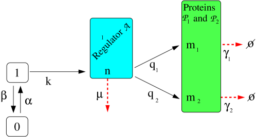
Refer to caption
Figure 8: The three-stage model of gene expression, with arbitrary partition of proteins.
Refer to caption
Figure 9: Comparison of the time evolution of the mean numbers ⟨m1βŸ©β€‹(t)delimited-⟨⟩subscriptπ‘š1𝑑\langle m_{1}\rangle(t), ⟨m2βŸ©β€‹(t)delimited-⟨⟩subscriptπ‘š2𝑑\langle m_{2}\rangle(t) for the two stage model (in red - for parameter values k=6.25π‘˜6.25k=6.25, ΞΌ=1πœ‡1\mu=1, q1=3subscriptπ‘ž13q_{1}=3, q2=5subscriptπ‘ž25q_{2}=5, Ξ³1=Ξ³2=2subscript𝛾1subscript𝛾22\gamma_{1}=\gamma_{2}=2) and three state model (in black - for parameter values Ξ±=2.5𝛼2.5\alpha=2.5, Ξ²=1.5𝛽1.5\beta=1.5, k1=10subscriptπ‘˜110k_{1}=10, ΞΌ=1πœ‡1\mu=1, q1=3subscriptπ‘ž13q_{1}=3, q2=5subscriptπ‘ž25q_{2}=5, Ξ³1=Ξ³2=2subscript𝛾1subscript𝛾22\gamma_{1}=\gamma_{2}=2). Analytical results (lines) are compared to numerical results (symbols). In the insert, we compare correlations between protein numbers for the two stage model (in red) and three stage model (in black). For the same parameter values, we plot the time evolution of (1+R)​C1,2​(t)1𝑅subscript𝐢12𝑑(1+R)C_{1,2}(t) (red) together with π’ž1,2​(t)subscriptπ’ž12𝑑{\cal C}_{1,2}(t) (black).

4 Conclusion

In this paper, we present a variation on the two-stage model including the arbitrary partition of protein and arbitrary time dependent parameters. The mechanism considered is similar to the one involved in alternative splicing [49]. Our aim was to develop an analytical approach leading to the time dependent generating function, based on the PPA-mapping, and which did not require knowledge of already known results. Constructed on a succession of transformations, our work simplifies the original problem to the analysis of two-states biological switches. As a consequence, a series of different reduced models emerges, with clear relations linking their respective generating functions. In particular we show how the kernel 𝒦jsubscript𝒦𝑗{\cal K}_{j} plays a important role in the final expression of the generating function. We show that the emerging hierarchy allows us to connect mean numbers and higher order moments between models. This leads to an explicit relation between correlation Ci,jsubscript𝐢𝑖𝑗C_{i,j} in the original model and mean protein number in model-2. For constant parameter values, we derived the exact time dependent expression of correlation Ci,jsubscript𝐢𝑖𝑗C_{i,j}. We note that particular cases such as Ξ³j=ΞΌsubscriptπ›Ύπ‘—πœ‡\gamma_{j}=\mu, Ξ³j=ΞΌ/2subscriptπ›Ύπ‘—πœ‡2\gamma_{j}=\mu/2 or Ξ³1+Ξ³2=ΞΌsubscript𝛾1subscript𝛾2πœ‡\gamma_{1}+\gamma_{2}=\mu have to be treated separately. However, in the stationary state this distinction vanishes as each function converges towards a common asymptotic expression. Considering constant parameters, for J=1𝐽1J=1 or for homogeneous degradation rates (Ξ³j=Ξ³subscript𝛾𝑗𝛾\gamma_{j}=\gamma βˆ€jfor-all𝑗\forall j), we show how our results reduce to the solution of two stage model. Finally, we show how results for arbitrary time dependent transition rates can be used to study models presenting parameter fluctuations induced by hidden random variable. We give an explicit example by extending our results for the mean and correlation to the three state model. In particular we show that promoter based regulation leads to higher protein-protein correlations π’ži,jβˆ—>Ci,jβˆ—subscriptsuperscriptπ’žπ‘–π‘—superscriptsubscript𝐢𝑖𝑗{\cal C}^{*}_{i,j}>C_{i,j}^{*}. The method presented here is applicable in other scenarios (with zero and first order reactions) and may be use as a guide in the study of other biological systems. We hope this methodology will contribute to the development of new analytical avenues for future research.

Acknowledgements

The authors would like to thanks the AMRC in Coventry and the Stat. Phys. Group in Nancy for their support and constant efforts to protect curiosity driven research. In particular, T. Platini extends his acknowledgements to K. Aujogue, R. Low, S. Mukherjee, S. Vantieghem and R. Kulkarni.

5 Appendix

5.1 From model-0 to model-1: a detailed derivation

In the following we aim to construct the original problem (model-0) starting with N𝑁N independent models, all identical to model-1. The derivation is presented for constant parameter, but could easily be extended to time dependent parameter. We will start with the definition of Ο•N;(ΞΈ,a,b)​(t)subscriptitalic-Ο•π‘πœƒπ‘Žπ‘π‘‘\phi_{N;(\theta,a,b)}(t): the probability of finding, in model-1, the biological switch in the state ΞΈπœƒ\theta together with aπ‘Ža and b𝑏b proteins of type 𝒫1subscript𝒫1{\cal P}_{1} and 𝒫2subscript𝒫2{\cal P}_{2} respectively. We continue by defining Ξ¦N​(n,m1,m2)subscriptΦ𝑁𝑛subscriptπ‘š1subscriptπ‘š2\Phi_{N}(n,m_{1},m_{2}) as the probability of finding amongst N𝑁N independent identical models (each labeled with subscript ν𝜈\nu) the total numbers of active switches n=βˆ‘Ξ½ΞΈΞ½π‘›subscript𝜈subscriptπœƒπœˆn=\sum_{\nu}\theta_{\nu} and proteins m1=βˆ‘Ξ½aΞ½subscriptπ‘š1subscript𝜈subscriptπ‘Žπœˆm_{1}=\sum_{\nu}a_{\nu}, m2=βˆ‘Ξ½bΞ½subscriptπ‘š2subscript𝜈subscriptπ‘πœˆm_{2}=\sum_{\nu}b_{\nu}. Finally when, taking the limit Nβ†’βˆžβ†’π‘N\rightarrow\infty, we will be able to show that limNβ†’βˆžΞ¦N​(t)subscript→𝑁subscriptΦ𝑁𝑑\lim_{N\rightarrow\infty}\Phi_{N}(t) obeys the master equation (​2.1​)italic-(2.1italic-)\eqref{eq_Master_eq}. In other words Pn,m1,m2=limNβ†’βˆžΞ¦N;(n,m1,m2)subscript𝑃𝑛subscriptπ‘š1subscriptπ‘š2subscript→𝑁subscriptΦ𝑁𝑛subscriptπ‘š1subscriptπ‘š2P_{n,m_{1},m_{2}}=\lim_{N\rightarrow\infty}\Phi_{N;(n,m_{1},m_{2})}.

To start let us try to keep notation as compact as possible by defining the flip operator F^^𝐹{\hat{F}} as the operator acting on the triplet (ΞΈ,a,b)πœƒπ‘Žπ‘(\theta,a,b) and such that F^​(ΞΈ,a,b)=(1βˆ’ΞΈ,a,b)^πΉπœƒπ‘Žπ‘1πœƒπ‘Žπ‘{\hat{F}}(\theta,a,b)=(1-\theta,a,b). In addition, we write A^Β±superscript^𝐴plus-or-minus{\hat{A}}^{\pm} and B^Β±superscript^𝐡plus-or-minus{\hat{B}}^{\pm} as the operators defined by

A^±​(ΞΈ,a,b)=(ΞΈ,aΒ±1,b),superscript^𝐴plus-or-minusπœƒπ‘Žπ‘πœƒplus-or-minusπ‘Ž1𝑏\displaystyle{\hat{A}}^{\pm}(\theta,a,b)=(\theta,a\pm 1,b), (85)
B^±​(ΞΈ,a,b)=(ΞΈ,a,bΒ±1).superscript^𝐡plus-or-minusπœƒπ‘Žπ‘πœƒπ‘Žplus-or-minus𝑏1\displaystyle{\hat{B}}^{\pm}(\theta,a,b)=(\theta,a,b\pm 1). (86)

Let Ο•N;(ΞΈ,a,b)​(t)subscriptitalic-Ο•π‘πœƒπ‘Žπ‘π‘‘\phi_{N;(\theta,a,b)}(t) be the probability distribution associated to model-1. It obeys the following equation

d​ϕN;(ΞΈ,a,b)d​t𝑑subscriptitalic-Ο•π‘πœƒπ‘Žπ‘π‘‘π‘‘\displaystyle\frac{d\phi_{N;(\theta,a,b)}}{dt} =\displaystyle= [θ​(k/N)+(1βˆ’ΞΈ)​μ]​ϕN;F^​(ΞΈ,a,b)delimited-[]πœƒπ‘˜π‘1πœƒπœ‡subscriptitalic-ϕ𝑁^πΉπœƒπ‘Žπ‘\displaystyle\left[\theta(k/N)+(1-\theta)\mu\right]\phi_{N;{\hat{F}}(\theta,a,b)}
+\displaystyle+ θ​q1​ϕN;A^βˆ’β€‹(ΞΈ,a,b)+θ​q2​ϕN;B^βˆ’β€‹(ΞΈ,a,b)πœƒsubscriptπ‘ž1subscriptitalic-ϕ𝑁superscript^π΄πœƒπ‘Žπ‘πœƒsubscriptπ‘ž2subscriptitalic-ϕ𝑁superscript^π΅πœƒπ‘Žπ‘\displaystyle\theta q_{1}\phi_{N;{\hat{A}}^{-}(\theta,a,b)}+\theta q_{2}\phi_{N;{\hat{B}}^{-}(\theta,a,b)}
+\displaystyle+ (a+1)​γ1​ϕN;A^+​(ΞΈ,a,b)+(b+1)​γ2​ϕN;B^+​(ΞΈ,a,b)π‘Ž1subscript𝛾1subscriptitalic-ϕ𝑁superscript^π΄πœƒπ‘Žπ‘π‘1subscript𝛾2subscriptitalic-ϕ𝑁superscript^π΅πœƒπ‘Žπ‘\displaystyle(a+1)\gamma_{1}\phi_{N;{\hat{A}}^{+}(\theta,a,b)}+(b+1)\gamma_{2}\phi_{N;{\hat{B}}^{+}(\theta,a,b)}
βˆ’\displaystyle- [(1βˆ’ΞΈ)​(k/N)+θ​μ+θ​q1+θ​q2+a​γ1+b​γ2]​ϕN;(ΞΈ,a,b).delimited-[]1πœƒπ‘˜π‘πœƒπœ‡πœƒsubscriptπ‘ž1πœƒsubscriptπ‘ž2π‘Žsubscript𝛾1𝑏subscript𝛾2subscriptitalic-Ο•π‘πœƒπ‘Žπ‘\displaystyle\left[(1-\theta)(k/N)+\theta\mu+\theta q_{1}+\theta q_{2}+a\gamma_{1}+b\gamma_{2}\right]\phi_{N;(\theta,a,b)}.

Considering N𝑁N independent but identical models, we define π•Šπ•Š{\mathbb{S}} as the set of triplets: π•Š={(ΞΈΞ½,aΞ½,bΞ½);Ξ½=1,2,…,N}{\mathbb{S}}=\{(\theta_{\nu},a_{\nu},b_{\nu});\nu=1,2,\ldots,N\}. Note that π•Šπ•Š{\mathbb{S}} gives a full description of the state of all N𝑁N independent reduced models. In addition, we will write θν​(π•Š)subscriptπœƒπœˆπ•Š\theta_{\nu}({\mathbb{S}}), aν​(π•Š)subscriptπ‘Žπœˆπ•Ša_{\nu}({\mathbb{S}}) and bν​(π•Š)subscriptπ‘πœˆπ•Šb_{\nu}({\mathbb{S}}) the variable ΞΈπœƒ\theta, aπ‘Ža and b𝑏b in the Ξ½t​hsuperscriptπœˆπ‘‘β„Ž\nu^{th} triplet of the set π•Šπ•Š{\mathbb{S}}. The definitions of the operator F^^𝐹{\hat{F}}, A^Β±superscript^𝐴plus-or-minus{\hat{A}}^{\pm} and B^Β±superscript^𝐡plus-or-minus{\hat{B}}^{\pm} are extended onto the set π•Šπ•Š{\mathbb{S}}. So that F^Ξ½subscript^𝐹𝜈{\hat{F}}_{\nu}, A^Ξ½Β±subscriptsuperscript^𝐴plus-or-minus𝜈{\hat{A}}^{\pm}_{\nu} and B^Ξ½Β±subscriptsuperscript^𝐡plus-or-minus𝜈{\hat{B}}^{\pm}_{\nu} act on the Ξ½t​hsuperscriptπœˆπ‘‘β„Ž\nu^{th} triplet of the set π•Šπ•Š{\mathbb{S}}, leaving all others unchanged. We can now define the overall probability Ο•N,π•Š=∏ν=1NΟ•N,(ΞΈΞ½,aΞ½,bΞ½)subscriptitalic-Ο•π‘π•Šsuperscriptsubscriptproduct𝜈1𝑁subscriptitalic-ϕ𝑁subscriptπœƒπœˆsubscriptπ‘Žπœˆsubscriptπ‘πœˆ\phi_{N,{\mathbb{S}}}=\prod_{\nu=1}^{N}\phi_{N,(\theta_{\nu},a_{\nu},b_{\nu})}, which evolution is governed by

dd​t​ϕN,π•Š=βˆ‘i=1NβˆΞ½β‰ iΟ•N,(ΞΈΞ½,aΞ½,bΞ½)​dd​t​ϕN,(ΞΈi,ai,bi).𝑑𝑑𝑑subscriptitalic-Ο•π‘π•Šsuperscriptsubscript𝑖1𝑁subscriptproductπœˆπ‘–subscriptitalic-ϕ𝑁subscriptπœƒπœˆsubscriptπ‘Žπœˆsubscriptπ‘πœˆπ‘‘π‘‘π‘‘subscriptitalic-ϕ𝑁subscriptπœƒπ‘–subscriptπ‘Žπ‘–subscript𝑏𝑖\displaystyle\frac{d}{dt}\phi_{N,{\mathbb{S}}}=\sum_{i=1}^{N}\prod_{\nu\neq i}\phi_{N,(\theta_{\nu},a_{\nu},b_{\nu})}\frac{d}{dt}\phi_{N,(\theta_{i},a_{i},b_{i})}. (88)

With a little bit of effort, the latter equation leads to

dd​t​ϕN,π•Šπ‘‘π‘‘π‘‘subscriptitalic-Ο•π‘π•Š\displaystyle\frac{d}{dt}\phi_{N,{\mathbb{S}}} =\displaystyle= k/Nβ€‹βˆ‘i{ΞΈi​(π•Š)​ϕN,F^iβ€‹π•Šβˆ’[1βˆ’ΞΈi​(π•Š)]​ϕN,π•Š}π‘˜π‘subscript𝑖subscriptπœƒπ‘–π•Šsubscriptitalic-ϕ𝑁subscript^πΉπ‘–π•Šdelimited-[]1subscriptπœƒπ‘–π•Šsubscriptitalic-Ο•π‘π•Š\displaystyle k/N\sum_{i}\left\{\theta_{i}({\mathbb{S}})\phi_{N,{\hat{F}}_{i}{\mathbb{S}}}-[1-\theta_{i}({\mathbb{S}})]\phi_{N,{\mathbb{S}}}\right\}
+\displaystyle+ ΞΌβ€‹βˆ‘i{[1βˆ’ΞΈi​(π•Š)]​ϕN,F^iβ€‹π•Šβˆ’ΞΈi​(π•Š)​ϕN,π•Š}πœ‡subscript𝑖delimited-[]1subscriptπœƒπ‘–π•Šsubscriptitalic-ϕ𝑁subscript^πΉπ‘–π•Šsubscriptπœƒπ‘–π•Šsubscriptitalic-Ο•π‘π•Š\displaystyle\mu\sum_{i}\left\{[1-\theta_{i}({\mathbb{S}})]\phi_{N,{\hat{F}}_{i}{\mathbb{S}}}-\theta_{i}({\mathbb{S}})\phi_{N,{\mathbb{S}}}\right\}
+\displaystyle+ q1β€‹βˆ‘iΞΈi​(π•Š)​{Ο•N,A^iβˆ’β€‹π•Šβˆ’Ο•N,π•Š}subscriptπ‘ž1subscript𝑖subscriptπœƒπ‘–π•Šsubscriptitalic-ϕ𝑁subscriptsuperscript^π΄π‘–π•Šsubscriptitalic-Ο•π‘π•Š\displaystyle q_{1}\sum_{i}\theta_{i}({\mathbb{S}})\left\{\phi_{N,{\hat{A}}^{-}_{i}{\mathbb{S}}}-\phi_{N,{\mathbb{S}}}\right\}
+\displaystyle+ q2β€‹βˆ‘iΞΈi​(π•Š)​{Ο•N,B^iβˆ’β€‹π•Šβˆ’Ο•N,π•Š}subscriptπ‘ž2subscript𝑖subscriptπœƒπ‘–π•Šsubscriptitalic-ϕ𝑁subscriptsuperscript^π΅π‘–π•Šsubscriptitalic-Ο•π‘π•Š\displaystyle q_{2}\sum_{i}\theta_{i}({\mathbb{S}})\left\{\phi_{N,{\hat{B}}^{-}_{i}{\mathbb{S}}}-\phi_{N,{\mathbb{S}}}\right\}
+\displaystyle+ Ξ³1β€‹βˆ‘i{[ai​(π•Š)+1]​ϕN,A^i+β€‹π•Šβˆ’ai​(π•Š)​ϕN,π•Š}subscript𝛾1subscript𝑖delimited-[]subscriptπ‘Žπ‘–π•Š1subscriptitalic-ϕ𝑁subscriptsuperscript^π΄π‘–π•Šsubscriptπ‘Žπ‘–π•Šsubscriptitalic-Ο•π‘π•Š\displaystyle\gamma_{1}\sum_{i}\left\{[a_{i}({\mathbb{S}})+1]\phi_{N,{\hat{A}}^{+}_{i}{\mathbb{S}}}-a_{i}({\mathbb{S}})\phi_{N,{\mathbb{S}}}\right\}
+\displaystyle+ Ξ³2β€‹βˆ‘i{[bi​(π•Š)+1]​ϕN,B^i+β€‹π•Šβˆ’bi​(π•Š)​ϕN,π•Š}.subscript𝛾2subscript𝑖delimited-[]subscriptπ‘π‘–π•Š1subscriptitalic-ϕ𝑁subscriptsuperscript^π΅π‘–π•Šsubscriptπ‘π‘–π•Šsubscriptitalic-Ο•π‘π•Š\displaystyle\gamma_{2}\sum_{i}\left\{[b_{i}({\mathbb{S}})+1]\phi_{N,{\hat{B}}^{+}_{i}{\mathbb{S}}}-b_{i}({\mathbb{S}})\phi_{N,{\mathbb{S}}}\right\}.

Moving forward, we define the probability distribution Ξ¦NsubscriptΦ𝑁\Phi_{N} as

Ξ¦N;(n,m1,m2)=βˆ‘π•ŠΟ•N;π•Šβ€‹Ξ”n{ΞΈΞ½}​Δm1{aΞ½}​Δm2{bΞ½},subscriptΦ𝑁𝑛subscriptπ‘š1subscriptπ‘š2subscriptπ•Šsubscriptitalic-Ο•π‘π•ŠsubscriptsuperscriptΞ”subscriptπœƒπœˆπ‘›subscriptsuperscriptΞ”subscriptπ‘Žπœˆsubscriptπ‘š1subscriptsuperscriptΞ”subscriptπ‘πœˆsubscriptπ‘š2\displaystyle\Phi_{N;(n,m_{1},m_{2})}=\sum_{{\mathbb{S}}}\phi_{N;{\mathbb{S}}}\Delta^{\{\theta_{\nu}\}}_{n}\Delta^{\{a_{\nu}\}}_{m_{1}}\Delta^{\{b_{\nu}\}}_{m_{2}}, (90)

where the constraint ΔΔ\Delta is defined by

Ξ”y{xΞ½}=δ​(βˆ‘Ξ½xΞ½,y),subscriptsuperscriptΞ”subscriptπ‘₯πœˆπ‘¦π›Ώsubscript𝜈subscriptπ‘₯πœˆπ‘¦\displaystyle\Delta^{\{x_{\nu}\}}_{y}=\delta\left(\sum_{\nu}x_{\nu},y\right), (91)

where δ𝛿\delta is the Kronecker symbol. To keep notations as compact as possible we write Ξ”(3)=Ξ”n{ΞΈΞ½}​Δm1{aΞ½}​Δm2{bΞ½}superscriptΞ”3subscriptsuperscriptΞ”subscriptπœƒπœˆπ‘›subscriptsuperscriptΞ”subscriptπ‘Žπœˆsubscriptπ‘š1subscriptsuperscriptΞ”subscriptπ‘πœˆsubscriptπ‘š2\Delta^{(3)}=\Delta^{\{\theta_{\nu}\}}_{n}\Delta^{\{a_{\nu}\}}_{m_{1}}\Delta^{\{b_{\nu}\}}_{m_{2}}. The master equation for the distribution Ξ¦NsubscriptΦ𝑁\Phi_{N} is

dd​t​ΦN,(n,m1,m2)𝑑𝑑𝑑subscriptΦ𝑁𝑛subscriptπ‘š1subscriptπ‘š2\displaystyle\frac{d}{dt}\Phi_{N,(n,m_{1},m_{2})} =\displaystyle= k/Nβ€‹βˆ‘π•ŠΞ”(3)β€‹βˆ‘i{ΞΈi​(π•Š)​ϕN,F^iβ€‹π•Šβˆ’[1βˆ’ΞΈi​(π•Š)]​ϕN,π•Š}π‘˜π‘subscriptπ•ŠsuperscriptΞ”3subscript𝑖subscriptπœƒπ‘–π•Šsubscriptitalic-ϕ𝑁subscript^πΉπ‘–π•Šdelimited-[]1subscriptπœƒπ‘–π•Šsubscriptitalic-Ο•π‘π•Š\displaystyle k/N\sum_{{\mathbb{S}}}\Delta^{(3)}\sum_{i}\left\{\theta_{i}({\mathbb{S}})\phi_{N,{\hat{F}}_{i}{\mathbb{S}}}-[1-\theta_{i}({\mathbb{S}})]\phi_{N,{\mathbb{S}}}\right\}
+\displaystyle+ ΞΌβ€‹βˆ‘π•ŠΞ”(3)β€‹βˆ‘i{[1βˆ’ΞΈi​(π•Š)]​ϕN,F^iβ€‹π•Šβˆ’ΞΈi​(π•Š)​ϕN,π•Š}πœ‡subscriptπ•ŠsuperscriptΞ”3subscript𝑖delimited-[]1subscriptπœƒπ‘–π•Šsubscriptitalic-ϕ𝑁subscript^πΉπ‘–π•Šsubscriptπœƒπ‘–π•Šsubscriptitalic-Ο•π‘π•Š\displaystyle\mu\sum_{{\mathbb{S}}}\Delta^{(3)}\sum_{i}\left\{[1-\theta_{i}({\mathbb{S}})]\phi_{N,{\hat{F}}_{i}{\mathbb{S}}}-\theta_{i}({\mathbb{S}})\phi_{N,{\mathbb{S}}}\right\}
+\displaystyle+ q1β€‹βˆ‘π•ŠΞ”(3)β€‹βˆ‘i{ΞΈi​(π•Š)​ϕN,A^iβˆ’β€‹π•Šβˆ’ΞΈi​(π•Š)​ϕN,π•Š}subscriptπ‘ž1subscriptπ•ŠsuperscriptΞ”3subscript𝑖subscriptπœƒπ‘–π•Šsubscriptitalic-ϕ𝑁subscriptsuperscript^π΄π‘–π•Šsubscriptπœƒπ‘–π•Šsubscriptitalic-Ο•π‘π•Š\displaystyle q_{1}\sum_{{\mathbb{S}}}\Delta^{(3)}\sum_{i}\left\{\theta_{i}({\mathbb{S}})\phi_{N,{\hat{A}}^{-}_{i}{\mathbb{S}}}-\theta_{i}({\mathbb{S}})\phi_{N,{\mathbb{S}}}\right\}
+\displaystyle+ q2β€‹βˆ‘π•ŠΞ”(3)β€‹βˆ‘i{ΞΈi​(π•Š)​ϕN,B^iβˆ’β€‹π•Šβˆ’ΞΈi​(π•Š)​ϕN,π•Š}subscriptπ‘ž2subscriptπ•ŠsuperscriptΞ”3subscript𝑖subscriptπœƒπ‘–π•Šsubscriptitalic-ϕ𝑁subscriptsuperscript^π΅π‘–π•Šsubscriptπœƒπ‘–π•Šsubscriptitalic-Ο•π‘π•Š\displaystyle q_{2}\sum_{{\mathbb{S}}}\Delta^{(3)}\sum_{i}\left\{\theta_{i}({\mathbb{S}})\phi_{N,{\hat{B}}^{-}_{i}{\mathbb{S}}}-\theta_{i}({\mathbb{S}})\phi_{N,{\mathbb{S}}}\right\}
+\displaystyle+ Ξ³1β€‹βˆ‘π•ŠΞ”(3)β€‹βˆ‘i{[ai​(π•Š)+1]​ϕN,A^i+β€‹π•Šβˆ’ai​(π•Š)​ϕN,π•Š}subscript𝛾1subscriptπ•ŠsuperscriptΞ”3subscript𝑖delimited-[]subscriptπ‘Žπ‘–π•Š1subscriptitalic-ϕ𝑁subscriptsuperscript^π΄π‘–π•Šsubscriptπ‘Žπ‘–π•Šsubscriptitalic-Ο•π‘π•Š\displaystyle\gamma_{1}\sum_{{\mathbb{S}}}\Delta^{(3)}\sum_{i}\left\{[a_{i}({\mathbb{S}})+1]\phi_{N,{\hat{A}}^{+}_{i}{\mathbb{S}}}-a_{i}({\mathbb{S}})\phi_{N,{\mathbb{S}}}\right\}
+\displaystyle+ Ξ³2β€‹βˆ‘π•ŠΞ”(3)β€‹βˆ‘i{[bi​(π•Š)+1]​ϕN,B^i+β€‹π•Šβˆ’bi​(π•Š)​ϕN,π•Š}.subscript𝛾2subscriptπ•ŠsuperscriptΞ”3subscript𝑖delimited-[]subscriptπ‘π‘–π•Š1subscriptitalic-ϕ𝑁subscriptsuperscript^π΅π‘–π•Šsubscriptπ‘π‘–π•Šsubscriptitalic-Ο•π‘π•Š\displaystyle\gamma_{2}\sum_{{\mathbb{S}}}\Delta^{(3)}\sum_{i}\left\{[b_{i}({\mathbb{S}})+1]\phi_{N,{\hat{B}}^{+}_{i}{\mathbb{S}}}-b_{i}({\mathbb{S}})\phi_{N,{\mathbb{S}}}\right\}.

Every sum, for which Ο•N;π•Šsubscriptitalic-Ο•π‘π•Š\phi_{N;{\mathbb{S}}} appears explicitly can be easily evaluated. As an example we give here the second term of the first line in the previous equation. Using the constraint Ξ”{ΞΈΞ½}superscriptΞ”subscriptπœƒπœˆ\Delta^{\{\theta_{\nu}\}}, which impose βˆ‘Ξ½ΞΈΞ½=nsubscript𝜈subscriptπœƒπœˆπ‘›\sum_{\nu}\theta_{\nu}=n, we have

βˆ‘π•ŠΞ”n{ΞΈΞ½}​Δm1{aΞ½}​Δm2{bΞ½}β€‹βˆ‘i[1βˆ’ΞΈi​(π•Š)]​ϕN,π•Šsubscriptπ•ŠsubscriptsuperscriptΞ”subscriptπœƒπœˆπ‘›subscriptsuperscriptΞ”subscriptπ‘Žπœˆsubscriptπ‘š1subscriptsuperscriptΞ”subscriptπ‘πœˆsubscriptπ‘š2subscript𝑖delimited-[]1subscriptπœƒπ‘–π•Šsubscriptitalic-Ο•π‘π•Š\displaystyle\sum_{{\mathbb{S}}}\Delta^{\{\theta_{\nu}\}}_{n}\Delta^{\{a_{\nu}\}}_{m_{1}}\Delta^{\{b_{\nu}\}}_{m_{2}}\sum_{i}[1-\theta_{i}({\mathbb{S}})]\phi_{N,{\mathbb{S}}} =\displaystyle= βˆ‘π•ŠΞ”n{ΞΈΞ½}​Δm1{aΞ½}​Δm2{bΞ½}​[Nβˆ’n]​ϕN,π•Šsubscriptπ•ŠsubscriptsuperscriptΞ”subscriptπœƒπœˆπ‘›subscriptsuperscriptΞ”subscriptπ‘Žπœˆsubscriptπ‘š1subscriptsuperscriptΞ”subscriptπ‘πœˆsubscriptπ‘š2delimited-[]𝑁𝑛subscriptitalic-Ο•π‘π•Š\displaystyle\sum_{{\mathbb{S}}}\Delta^{\{\theta_{\nu}\}}_{n}\Delta^{\{a_{\nu}\}}_{m_{1}}\Delta^{\{b_{\nu}\}}_{m_{2}}[N-n]\phi_{N,{\mathbb{S}}} (93)
=\displaystyle= (Nβˆ’n)​ΦN,(n,m1,m2).𝑁𝑛subscriptΦ𝑁𝑛subscriptπ‘š1subscriptπ‘š2\displaystyle(N-n)\Phi_{N,(n,m_{1},m_{2})}.

When Ο•N,π•Šsubscriptitalic-Ο•π‘π•Š\phi_{N,{\mathbb{S}}} does not appear explicitly we need to re-labeled the sum over π•Šπ•Š{\mathbb{S}}. As an example we present details to the calculation of the first term of the first line in which we have Ο•N,F^iβ€‹π•Šsubscriptitalic-ϕ𝑁subscript^πΉπ‘–π•Š\phi_{N,{\hat{F}}_{i}{\mathbb{S}}}. Defining π•Š~=F^iβ€‹π•Š~π•Šsubscript^πΉπ‘–π•Š\tilde{\mathbb{S}}={\hat{F}}_{i}{\mathbb{S}} we have F^iβ€‹π•Š~=π•Šsubscript^𝐹𝑖~π•Šπ•Š{\hat{F}}_{i}\tilde{\mathbb{S}}={\mathbb{S}} so that

ΞΈj​(π•Š)=ΞΈj​(F^iβ€‹π•Š~)={θν​(π•Š~),ifiβ‰ Ξ½1βˆ’ΞΈi​(π•Š~),ifi=Ξ½.subscriptπœƒπ‘—π•Šsubscriptπœƒπ‘—subscript^𝐹𝑖~π•Šcasessubscriptπœƒπœˆ~π•Šifπ‘–πœˆ1subscriptπœƒπ‘–~π•Šifπ‘–πœˆ\theta_{j}({\mathbb{S}})=\theta_{j}({\hat{F}}_{i}\tilde{\mathbb{S}})=\left\{\begin{array}[]{ccc}\theta_{\nu}(\tilde{\mathbb{S}}),&{\text{if}}&i\neq\nu\\ 1-\theta_{i}(\tilde{\mathbb{S}}),&{\text{if}}&i=\nu.\end{array}\right. (94)

In relabelling π•Šπ•Š{\mathbb{S}} to π•Š~~π•Š\tilde{\mathbb{S}} the expression of Ξ”{ΞΈΞ½}superscriptΞ”subscriptπœƒπœˆ\Delta^{\{\theta_{\nu}\}} has changed. To keep track of this change we will replace Ξ”{ΞΈΞ½}β†’Ξ”~{ΞΈΞ½}β†’superscriptΞ”subscriptπœƒπœˆsuperscript~Ξ”subscriptπœƒπœˆ\Delta^{\{\theta_{\nu}\}}\rightarrow\tilde{\Delta}^{\{\theta_{\nu}\}} where

Ξ”n{ΞΈΞ½}subscriptsuperscriptΞ”subscriptπœƒπœˆπ‘›\displaystyle\Delta^{\{\theta_{\nu}\}}_{n} =\displaystyle= δ​(βˆ‘Ξ½ΞΈΞ½β€‹(π•Š),n)=δ​(βˆ‘Ξ½ΞΈΞ½β€‹(π•Š~)+1βˆ’2​θi​(π•Š~),n)=Ξ”~n{ΞΈΞ½}𝛿subscript𝜈subscriptπœƒπœˆπ•Šπ‘›π›Ώsubscript𝜈subscriptπœƒπœˆ~π•Š12subscriptπœƒπ‘–~π•Šπ‘›subscriptsuperscript~Ξ”subscriptπœƒπœˆπ‘›\displaystyle\delta\left(\sum_{\nu}\theta_{\nu}({\mathbb{S}}),n\right)=\delta\left(\sum_{\nu}\theta_{\nu}(\tilde{\mathbb{S}})+1-2\theta_{i}(\tilde{\mathbb{S}}),n\right)=\tilde{\Delta}^{\{\theta_{\nu}\}}_{n} (95)

It follows that

βˆ‘i=1Nβˆ‘π•ŠΞ”n{ΞΈΞ½}​Δm1{aΞ½}​Δm2{bΞ½}​θi​(π•Š)​ϕN,F^iβ€‹π•Š=βˆ‘i=1Nβˆ‘π•Š~Ξ”~n{ΞΈΞ½}​Δm1{aΞ½}​Δm2{bΞ½}​[1βˆ’ΞΈi​(π•Š~)]​ϕN,π•Š~.superscriptsubscript𝑖1𝑁subscriptπ•ŠsubscriptsuperscriptΞ”subscriptπœƒπœˆπ‘›subscriptsuperscriptΞ”subscriptπ‘Žπœˆsubscriptπ‘š1subscriptsuperscriptΞ”subscriptπ‘πœˆsubscriptπ‘š2subscriptπœƒπ‘–π•Šsubscriptitalic-ϕ𝑁subscript^πΉπ‘–π•Šsuperscriptsubscript𝑖1𝑁subscript~π•Šsubscriptsuperscript~Ξ”subscriptπœƒπœˆπ‘›subscriptsuperscriptΞ”subscriptπ‘Žπœˆsubscriptπ‘š1subscriptsuperscriptΞ”subscriptπ‘πœˆsubscriptπ‘š2delimited-[]1subscriptπœƒπ‘–~π•Šsubscriptitalic-ϕ𝑁~π•Š\displaystyle\sum_{i=1}^{N}\sum_{{\mathbb{S}}}\Delta^{\{\theta_{\nu}\}}_{n}\Delta^{\{a_{\nu}\}}_{m_{1}}\Delta^{\{b_{\nu}\}}_{m_{2}}\theta_{i}({\mathbb{S}})\phi_{N,{\hat{F}}_{i}{\mathbb{S}}}=\sum_{i=1}^{N}\sum_{\tilde{\mathbb{S}}}\tilde{\Delta}^{\{\theta_{\nu}\}}_{n}\Delta^{\{a_{\nu}\}}_{m_{1}}\Delta^{\{b_{\nu}\}}_{m_{2}}[1-\theta_{i}(\tilde{\mathbb{S}})]\phi_{N,\tilde{\mathbb{S}}}.

Note that the only elements which will contribute are such that ΞΈi​(π•Š~)=0subscriptπœƒπ‘–~π•Š0\theta_{i}(\tilde{\mathbb{S}})=0, which allows us to write

Ξ”~n{ΞΈj}=δ​(βˆ‘Ξ½ΞΈΞ½β€‹(π•Š~),(nβˆ’1)).subscriptsuperscript~Ξ”subscriptπœƒπ‘—π‘›π›Ώsubscript𝜈subscriptπœƒπœˆ~π•Šπ‘›1\displaystyle\tilde{\Delta}^{\{\theta_{j}\}}_{n}=\delta\left(\sum_{\nu}\theta_{\nu}(\tilde{\mathbb{S}}),(n-1)\right). (97)

Finally, we are able to express the first summation in term of Ξ¦N,(n,m1,m2)subscriptΦ𝑁𝑛subscriptπ‘š1subscriptπ‘š2\Phi_{N,(n,m_{1},m_{2})}:

βˆ‘i=1Nβˆ‘π•ŠΞ”n{ΞΈΞ½}​Δm1{aΞ½}​Δm2{bΞ½}​θi​(π•Š)​ϕN,F^iβ€‹π•Š=[Nβˆ’(nβˆ’1)]​ϕN,(nβˆ’1,m1,m2).superscriptsubscript𝑖1𝑁subscriptπ•ŠsubscriptsuperscriptΞ”subscriptπœƒπœˆπ‘›subscriptsuperscriptΞ”subscriptπ‘Žπœˆsubscriptπ‘š1subscriptsuperscriptΞ”subscriptπ‘πœˆsubscriptπ‘š2subscriptπœƒπ‘–π•Šsubscriptitalic-ϕ𝑁subscript^πΉπ‘–π•Šdelimited-[]𝑁𝑛1subscriptitalic-ϕ𝑁𝑛1subscriptπ‘š1subscriptπ‘š2\displaystyle\sum_{i=1}^{N}\sum_{{\mathbb{S}}}\Delta^{\{\theta_{\nu}\}}_{n}\Delta^{\{a_{\nu}\}}_{m_{1}}\Delta^{\{b_{\nu}\}}_{m_{2}}\theta_{i}({\mathbb{S}})\phi_{N,{\hat{F}}_{i}{\mathbb{S}}}=[N-(n-1)]\phi_{N,(n-1,m_{1},m_{2})}. (98)

Proceeding along the same line for every summation symbol we have

dd​t​ΦN,(n,m1,m2)𝑑𝑑𝑑subscriptΦ𝑁𝑛subscriptπ‘š1subscriptπ‘š2\displaystyle\frac{d}{dt}\Phi_{N,(n,m_{1},m_{2})} =\displaystyle= k​[1βˆ’(nβˆ’1)N]​ΦN,(nβˆ’1,m1,m2)βˆ’k​[1βˆ’nN]​ΦN,(n,m1,m2)π‘˜delimited-[]1𝑛1𝑁subscriptΦ𝑁𝑛1subscriptπ‘š1subscriptπ‘š2π‘˜delimited-[]1𝑛𝑁subscriptΦ𝑁𝑛subscriptπ‘š1subscriptπ‘š2\displaystyle k\left[1-\frac{(n-1)}{N}\right]\Phi_{N,(n-1,m_{1},m_{2})}-k\left[1-\frac{n}{N}\right]\Phi_{N,(n,m_{1},m_{2})}
+\displaystyle+ μ​(n+1)​ΦN,(n+1,m1,m2)βˆ’ΞΌβ€‹n​ΦN,(n,m1,m2)πœ‡π‘›1subscriptΦ𝑁𝑛1subscriptπ‘š1subscriptπ‘š2πœ‡π‘›subscriptΦ𝑁𝑛subscriptπ‘š1subscriptπ‘š2\displaystyle\mu(n+1)\Phi_{N,(n+1,m_{1},m_{2})}-\mu n\Phi_{N,(n,m_{1},m_{2})}
+\displaystyle+ q1​n​ΦN,(n,m1βˆ’1,m2)βˆ’q1​n​ΦN,(n,m1,m2)subscriptπ‘ž1𝑛subscriptΦ𝑁𝑛subscriptπ‘š11subscriptπ‘š2subscriptπ‘ž1𝑛subscriptΦ𝑁𝑛subscriptπ‘š1subscriptπ‘š2\displaystyle q_{1}n\Phi_{N,(n,m_{1}-1,m_{2})}-q_{1}n\Phi_{N,(n,m_{1},m_{2})}
+\displaystyle+ q1​n​ΦN,(n,m1,m2βˆ’1)βˆ’q2​n​ΦN,(n,m1,m2)subscriptπ‘ž1𝑛subscriptΦ𝑁𝑛subscriptπ‘š1subscriptπ‘š21subscriptπ‘ž2𝑛subscriptΦ𝑁𝑛subscriptπ‘š1subscriptπ‘š2\displaystyle q_{1}n\Phi_{N,(n,m_{1},m_{2}-1)}-q_{2}n\Phi_{N,(n,m_{1},m_{2})}
+\displaystyle+ Ξ³1​[m1+1]​ΦN,(n,m1+1,m2)βˆ’Ξ³1​m1​ΦN,(n,m1,m2)subscript𝛾1delimited-[]subscriptπ‘š11subscriptΦ𝑁𝑛subscriptπ‘š11subscriptπ‘š2subscript𝛾1subscriptπ‘š1subscriptΦ𝑁𝑛subscriptπ‘š1subscriptπ‘š2\displaystyle\gamma_{1}[m_{1}+1]\Phi_{N,(n,m_{1}+1,m_{2})}-\gamma_{1}m_{1}\Phi_{N,(n,m_{1},m_{2})}
+\displaystyle+ Ξ³2​[m2+1]​ΦN,(n,m1,m2+1)βˆ’Ξ³2​m2​ΦN,(n,m1,m2).subscript𝛾2delimited-[]subscriptπ‘š21subscriptΦ𝑁𝑛subscriptπ‘š1subscriptπ‘š21subscript𝛾2subscriptπ‘š2subscriptΦ𝑁𝑛subscriptπ‘š1subscriptπ‘š2\displaystyle\gamma_{2}[m_{2}+1]\Phi_{N,(n,m_{1},m_{2}+1)}-\gamma_{2}m_{2}\Phi_{N,(n,m_{1},m_{2})}.

Taking the limit Nβ†’βˆžβ†’π‘N\rightarrow\infty, we see that the latter equation converges towards the master equation (2.1). In other words Pn,m1,m2=limNβ†’βˆžΞ¦N;(n,m1,m2)subscript𝑃𝑛subscriptπ‘š1subscriptπ‘š2subscript→𝑁subscriptΦ𝑁𝑛subscriptπ‘š1subscriptπ‘š2P_{n,m_{1},m_{2}}=\lim_{N\rightarrow\infty}\Phi_{N;(n,m_{1},m_{2})}, from which it naturally follow G(0)=limNβ†’βˆž(GN(1))Nsuperscript𝐺0subscript→𝑁superscriptsubscriptsuperscript𝐺1𝑁𝑁G^{(0)}=\lim_{N\rightarrow\infty}\left(G^{(1)}_{N}\right)^{N}.

5.2 Large time approximation

The large time approximation, for one protein type only, is obtained by writting r=ΞΌ/Ξ³π‘Ÿπœ‡π›Ύr=\mu/\gamma, Ξ΄=q​(zβˆ’1)/Ξ³π›Ώπ‘žπ‘§1𝛾\delta=q(z-1)/\gamma and Ο΅=eβˆ’Ξ³β€‹titalic-Ο΅superscript𝑒𝛾𝑑\epsilon=e^{-\gamma t} so that

(zβˆ’1)​A=δ​kΞ³β€‹βˆ«Ο΅1duβ€‹βˆ«u1dv​Ω​(u,v),𝑧1π΄π›Ώπ‘˜π›Ύsuperscriptsubscriptitalic-Ο΅1differential-d𝑒superscriptsubscript𝑒1differential-d𝑣Ω𝑒𝑣\displaystyle(z-1)A=\delta\frac{k}{\gamma}\int_{\epsilon}^{1}\mathrm{d}u\int_{u}^{1}\mathrm{d}v\ \Omega(u,v), (100)

with

Ω​(u,v)=urβˆ’1vr​exp⁑[δ​(z)​(vβˆ’u)].Ω𝑒𝑣superscriptπ‘’π‘Ÿ1superscriptπ‘£π‘Ÿπ›Ώπ‘§π‘£π‘’\displaystyle\Omega(u,v)=\frac{u^{r-1}}{v^{r}}\exp\left[{\delta(z)(v-u)}\right]. (101)

Using the Taylor expansion leads to

(zβˆ’1)​A𝑧1𝐴\displaystyle(z-1)A =\displaystyle= δ​kΞ³β€‹βˆ‘n=0βˆžβˆ‘m=0∞(βˆ’1)m​δn+mm!​n!β€‹βˆ«Ο΅1du​um+rβˆ’1β€‹βˆ«u1dv​vnβˆ’r,π›Ώπ‘˜π›Ύsuperscriptsubscript𝑛0superscriptsubscriptπ‘š0superscript1π‘šsuperscriptπ›Ώπ‘›π‘šπ‘šπ‘›superscriptsubscriptitalic-Ο΅1differential-d𝑒superscriptπ‘’π‘šπ‘Ÿ1superscriptsubscript𝑒1differential-d𝑣superscriptπ‘£π‘›π‘Ÿ\displaystyle\delta\frac{k}{\gamma}\sum_{n=0}^{\infty}\sum_{m=0}^{\infty}\frac{(-1)^{m}\delta^{n+m}}{m!n!}\int_{\epsilon}^{1}\mathrm{d}u\ u^{m+r-1}\int_{u}^{1}\mathrm{d}v\ v^{n-r}, (102)

for which there is no particular problem unless in the last integral we have nβˆ’r=βˆ’1π‘›π‘Ÿ1n-r=-1 for some value of n𝑛n. Avoiding this situation, by choosing rβˆ‰β„•π‘Ÿβ„•r\notin\mathbb{N}, leads to

(zβˆ’1)​A=IF𝑧1𝐴subscript𝐼𝐹\displaystyle(z-1)A=I_{F} +\displaystyle+ δ​kΞ³β€‹βˆ‘n=0βˆžβˆ‘m=0∞(βˆ’1)m​δn+mm!​n!​1nβˆ’r+1π›Ώπ‘˜π›Ύsuperscriptsubscript𝑛0superscriptsubscriptπ‘š0superscript1π‘šsuperscriptπ›Ώπ‘›π‘šπ‘šπ‘›1π‘›π‘Ÿ1\displaystyle\delta\frac{k}{\gamma}\sum_{n=0}^{\infty}\sum_{m=0}^{\infty}\frac{(-1)^{m}\delta^{n+m}}{m!n!}\frac{1}{n-r+1} (103)
Γ—\displaystyle\times [1n+m+1​ϡn+m+1βˆ’1m+r​ϡm+r],delimited-[]1π‘›π‘š1superscriptitalic-Ο΅π‘›π‘š11π‘šπ‘Ÿsuperscriptitalic-Ο΅π‘šπ‘Ÿ\displaystyle\left[\frac{1}{n+m+1}\epsilon^{n+m+1}-\frac{1}{m+r}\epsilon^{m+r}\right],

with

IFsubscript𝐼𝐹\displaystyle I_{F} =\displaystyle= δ​kΞ³β€‹βˆ‘ΞΊ=0∞δκκ+1β€‹βˆ‘m=0ΞΊ(βˆ’1)mm!​(ΞΊβˆ’m)!​1(m+r)=δ​kΞ³β€‹βˆ‘ΞΊ=0∞δκκ+1​(rβˆ’1)!(r+ΞΊ)!π›Ώπ‘˜π›Ύsuperscriptsubscriptπœ…0superscriptπ›Ώπœ…πœ…1superscriptsubscriptπ‘š0πœ…superscript1π‘šπ‘šπœ…π‘š1π‘šπ‘Ÿπ›Ώπ‘˜π›Ύsuperscriptsubscriptπœ…0superscriptπ›Ώπœ…πœ…1π‘Ÿ1π‘Ÿπœ…\displaystyle\delta\frac{k}{\gamma}\sum_{\kappa=0}^{\infty}\frac{\delta^{\kappa}}{\kappa+1}\sum_{m=0}^{\kappa}\frac{(-1)^{m}}{m!(\kappa-m)!}\frac{1}{(m+r)}=\delta\frac{k}{\gamma}\sum_{\kappa=0}^{\infty}\frac{\delta^{\kappa}}{\kappa+1}\frac{(r-1)!}{(r+\kappa)!} (104)
=\displaystyle= kΞΌβ€‹βˆ«0Ξ΄ds1​F1​[1,r+1,s].π‘˜πœ‡superscriptsubscript0𝛿differential-dsubscript𝑠1subscript𝐹11π‘Ÿ1𝑠\displaystyle\frac{k}{\mu}\int_{0}^{\delta}\mathrm{d}s\ _{1}F_{1}[1,r+1,s].

Keeping the lowest order in Ο΅italic-Ο΅\epsilon we get (zβˆ’1)​A≃IF+hsimilar-to-or-equals𝑧1𝐴subscriptπΌπΉβ„Ž(z-1)A\simeq I_{F}+h with

h={δ​kγ​ϡ1βˆ’rr>1βˆ’Ξ΄β€‹kγ​ϡrrβ€‹βˆ‘n=0∞δnn!​1nβˆ’r+1r<1.β„Žcasesπ›Ώπ‘˜π›Ύitalic-Ο΅1π‘Ÿπ‘Ÿ1π›Ώπ‘˜π›Ύsuperscriptitalic-Ο΅π‘Ÿπ‘Ÿsuperscriptsubscript𝑛0superscript𝛿𝑛𝑛1π‘›π‘Ÿ1π‘Ÿ1h=\left\{\begin{array}[]{cc}\delta\frac{k}{\gamma}\frac{\epsilon}{1-r}&r>1\\ -\delta\frac{k}{\gamma}\frac{\epsilon^{r}}{r}\sum_{n=0}^{\infty}\frac{\delta^{n}}{n!}\frac{1}{n-r+1}&r<1.\end{array}\right. (105)

It follows that G(0)​(z,t)≃Gβˆ—β€‹(z)​H​(z,t)similar-to-or-equalssuperscript𝐺0𝑧𝑑superscript𝐺𝑧𝐻𝑧𝑑G^{(0)}(z,t)\simeq G^{*}(z)H(z,t), with H=eh𝐻superscriptπ‘’β„ŽH=e^{h} as presented in equation (65). Going back to equation (102), we can work with r=1π‘Ÿ1r=1 (ΞΌ=Ξ³πœ‡π›Ύ\mu=\gamma). In this case, when keeping terms of order Ο΅italic-Ο΅\epsilon and ϡ​ln⁑(Ο΅)italic-Ο΅italic-Ο΅\epsilon\ln(\epsilon) we get :

h=βˆ’Ξ΄β€‹kμ​eβˆ’ΞΌβ€‹t​(μ​t+βˆ‘n=1∞δnnΓ—n!).β„Žπ›Ώπ‘˜πœ‡superscriptπ‘’πœ‡π‘‘πœ‡π‘‘superscriptsubscript𝑛1superscript𝛿𝑛𝑛𝑛h=-\delta\frac{k}{\mu}e^{-\mu t}\left(\mu t+\sum_{n=1}^{\infty}\frac{\delta^{n}}{n\times n!}\right). (106)

Under the following approximation we get ⟨mβŸ©β€‹(t)/⟨mβŸ©βˆ—β‰ƒ1βˆ’ΞΌβ€‹t​eβˆ’ΞΌβ€‹tsimilar-to-or-equalsdelimited-βŸ¨βŸ©π‘šπ‘‘superscriptdelimited-βŸ¨βŸ©π‘š1πœ‡π‘‘superscriptπ‘’πœ‡π‘‘\langle m\rangle(t)/\langle m\rangle^{*}\simeq 1-\mu te^{-\mu t} in agreement with the long time limit of equation (5).

6 Bibliography

References

  • [1] Ko M S, Nakauchi H, and Takahashi N 1990 The dose dependence of glucocorticoid-inducible gene expression results from changes in the number of transcriptionally active templates EMBO J. 9 2835-2842
  • [2] Ko M S 1991 A stochastic model for gene induction J. Theor. Biol. 153 181-194
  • [3] Raj A and van Oudenaarden A 2008 Nature, nurture, or chance: Stochastic gene expression and its consequences Cell 135 216-226
  • [4] Larson D R, Singer R H, and Zenklusen D 2009 A single molecule view of gene expression Trends Cell Biol. 19 630
  • [5] Huang S 2009 Non-genetic heterogeneity of cells in development: more than just noise Development 136 3853-62
  • [6] Eldar A and Elowitz M B 2010 Functional roles for noise in genetic circuits Nature 467 167
  • [7] Lionnet T and Singer R H 2012 Transcription goes digital EMBO reports 13(4) 313-21
  • [8] Van Kampen N G 2007 Stochastic Processes in Physics and Chemistry, 3rd Edition North Holland.
  • [9] Lobner-Olesen A 1999 Distribution of minichromosomes in individual Escherichia coli cells: implications for replication control EMBO J. 18(6) 1712-21
  • [10] Becskei A, Seraphin B and Serrano L 2001 Positive feedback in eukaryotic gene networks: cell differentiation by graded to binary response conversion EMBO J. 20(10) 2528-35
  • [11] Elowitz M B, Levine A J, Siggia E D and Swain P S 2002 Stochastic Gene Expression in a Single Cell Science 297 1183
  • [12] Ozbudak E M, Thattai M, Kurtser I, Grossman A D and van Oudenaarden A 2002 Regulation of noise in the expression of a single gene Nature Genetics 31 69 - 73
  • [13] Blake W J, Kaern M, Cantor C R, Collins J J 2003 Noise in eukaryotic gene expression Nature 422 633-637
  • [14] Acar M, Becskei A and van Oudenaarden A 2005 Enhancement of cellular memory by reducing stochastic transitions Nature 435 228-232
  • [15] Balazsi G, van Oudenaarden A and Collins J J 2011 Cellular decision making and biological noise: from microbes to mammals Cell 144(6) 910-25
  • [16] Nevozhay D, Adams R M, Murphy K F, Josic K and Balazsi G 2009 Negative autoregulation linearizes the dose-response and suppresses the heterogeneity of gene expression PNAS 106 (13) 5123-8
  • [17] Golding I, Paulsson J, Zawilski S M and Cox E C 2005 Real-time kinetics of gene activity in individual bacteria Cell 123 (6) 1025-1036
  • [18] Raj A, Peskin C S, Tranchina D, Vargas D Y and Tyagi S 2006 Stochastic mRNA synthesis in mammalian cells PLoS Biol 4(10) e309
  • [19] Taniguchi Y, Choi P J, Li G W, Chen H, Babu M, Hearn J, Emili A and Xie X S 2010 Quantifying E. coli proteome and transcriptome with single-molecule sensitivity in single cells Science 329 533
  • [20] Ferguson M, Le Coq D, Jules M, Aymerich S, Radulescu O, Declerck N and Royer CA 2012 Reconciling molecular regulatory mechanisms with noise patterns of bacterial metabolic promoters in induced and repressed states PNAS 109 155
  • [21] Peccoud J, and Ycart B 1995 Markovian modeling of gene-product synthesis Theoret. Popul. Biol. 48 222
  • [22] Hasty J, Pradines J, Dolnik M and Collins J J 2000 Noise-based switches and amplifiers for gene expression PNAS 97 (5) 2075-2080
  • [23] Paulsson J 2004 Summing up the noise in gene networks Nature (London) 427 415
  • [24] Karmakar R and Bose I, 2004 Graded and binary responses in stochastic gene expression Physical Biology 1 (4)
  • [25] Hornos J E M, Schultz D, Innocentini G C, Wang J, Walczak A M, Onuchic J N and Wolynes P G 2005 Self-regulating gene: an exact solution Phys. Rev. E 72 051907
  • [26] Friedman N, Cai L and Xie X S 2006 Linking stochastic dynamics to population distribution: an analytical framework of gene expression Phys. Rev. Lett. 97 168302
  • [27] Okabe Y, Yagi Y and Sasai M 2007 Effects of the DNA state fluctuation on single-cell dynamics of self-regulating gene J. Chem. Phys. 127 105107
  • [28] Ramos A F, Innocentini G C and Hornos J E 2011 Exact time-dependent solutions for a self-regulating gene Phys. Rev. E 83 062902
  • [29] Zhang J, Chen L and Zhou T 2012 Analytical distribution and tunability of noise in a model of promoter progress Biophysical Journal 102 (6) 1247-1257
  • [30] McAdams H and Arkin A 1997 Stochastic mechanisms in gene expression PNAS 94 814-819
  • [31] Coulon A, Gandrillon A, and Beslon G 2010 On the spontaneous stochastic dynamics of a single gene: complexity of the molecular interplay at the promoter BMC System Biology 4 2
  • [32] Kepler T B and Elston T C 2001 Stochasticity in transcriptional regulation: origins, consequences, and mathematical representations Biophys J. 81 (6) 3116-3136
  • [33] Paulsson J 2005 Models of Stochastic Gene Expression Phys. Life Rev. 2 157-175
  • [34] Paszek P 2007 Modeling stochasticity in gene regulation: characterization in the terms of the underlying distribution function Bull Math Biol. 69 (5) 1567-601
  • [35] Shahezaei V and Swain P S 2008 Analytical distributions for stochastic gene expression PNAS 105 (45) 17256-17261
  • [36] Iyer-Biswas S, Hayot F and Jayaprakash C 2009 Stochasticity of gene products from transcriptional pulsing Phys. Rev. E 79 031911
  • [37] Bokes P, King J R, Wood A T and Loose M 2012 Exact and approximate distributions of protein and mRNA levels in the low-copy regime of gene expression J. Math. Biol. 64 829-854
  • [38] Pedraza J M and Paulsson J 2008 Effects of molecular memory and bursting on fluctuations in gene expression Science 319 339
  • [39] Stinchcombe A R, Peskin C S and Tranchina D 2012 Population density approach for discrete mRNA distributions in generalized switching models for stochastic gene expression Phys. Rev. E 85 061919
  • [40] Thattai M and van Oudenaarden A 2001 Intrinsic noise in gene regulatory networks PNAS 98 (15) 8614-8619
  • [41] Xu B L and Tao Y 2006 External noise and feedback regulation: steady-state statistics of auto-regulatory genetic network J. Theor. Biol. 243 214
  • [42] Kumar N, Platini T and Kulkarni R V 2014 Exact distributions for stochastic gene expression models with bursting and feedback Phys. Rev. Lett. 113 268105
  • [43] Yu J, Xiao J, Ren X, Lao K and Xie X S 2006 Probing gene expression in live cells, one protein molecule at a time Science 311
  • [44] Suter D M, Molina N, Gatfield D, Schneider K, Schibler U and Naef F 2011 Mammalian genes are transcribed with widely different bursting kinetics Science 332 472
  • [45] Piatkevich K D, Lionnet T, Singer R H and Verkhusha V V 2011 Modern fluorescent proteins and imaging technologies to study gene expression, nuclear localization, and dynamics Curr. Opin. Cell. Biol. 23 310
  • [46] Lionnet T, Czaplinski K, Darzacq X, Shav-Tal Y, Wells A L, Chao J A, Park H Y, de Turris V, Lopez-Jones M and Singer RH 2011 A transgenic mouse for in vivo detection of endogenous labeled mRNA Nat. Methods 8 165
  • [47] Pendar H, Platini T and Kulkarni R V 2013 Exact protein distributions for stochastic models of gene expression using partitioning of Poisson processes Phys. Rev. E 87 042720
  • [48] Kulkarni R 2014 private communication
  • [49] Wang Q and Zhou T 2014 Alternative-splicing-mediated gene expression Phys. Rev. E 89 012713
  • [50] Modrek B and Lee C 2002 A genomic view of alternative splicing. Nat Genet. (1):13-9
  • [51] Black D L 2000 Protein diversity from alternative splicing: a challenge for bioinformatics and post-genome biology Cell 103 (3) 367-70
  • [52] Graveley B R 2001 Alternative splicing: increasing diversity in the proteomic world Trends Genet. (2): 100-7
  • [53] Grabowski P J and Black D L 2001 Alternative RNA splicing in the nervous system Prog. Neurobiol. 65(3):289-308
  • [54] Black D L Mechanisms of alternative pre-messenger RNA splicing 2003 Annu Rev Biochem. 72: 291-336
  • [55] Lesta I, et al., 2008 IEEE T Circuits-I 53 189-200
  • [56] Gadgil C, Lee C H and Othmer H G 2005 A stochastic analysis of first-order reaction networks Bull Math Biol 67: 901-946
  • [57] Singh A and Hespanha J P 2007 A derivative matching approach to moment closure for the stochastic logistic model Bull Math Biol 69 1909-1925
  • [58] Mugler A, Walczak A M and Wiggins C H 2010 Information-optimal transcriptional response to oscillatory driving Phys. Rev. Lett 105 058101
  • [59] Jedrak J and Ochab-Marcinek A 2016 Time-dependent solutions for a stochastic model of gene expression with molecule production in the form of a compound Poisson process Phys. Rev. E 94 032401
  • [60] Dattani J and Barahona M 2017 Stochastic models of gene transcription with upstream drives: exact solution and sample path characterization J. R. Soc. Interface 14 (126) 20160833
  • [61] Jahnke T and Huisinga W 2007 Solving the chemical master equation for monomolecular reactions systems analytically J of Math Biol 54 1 1-26
  • [62] Anderson D F, Craciun G and Kurtz T G 2010 Product-form stationary distributions for deficiency zero chemical reaction networks Bull of Math Biol 72 8 1947-1970
  • [63] Anderson D F and Cotter S L 2010 Product-form stationary distributions for deficiency zero networks with non-mass action kinetics Bull of Math Biol 78 12 2390-2407