Clustering For Point Pattern Data

Abstract

Clustering is one of the most common unsupervised learning tasks in machine learning and data mining. Clustering algorithms have been used in a plethora of applications across several scientific fields. However, there has been limited research in the clustering of point patterns – sets or multi-sets of unordered elements – that are found in numerous applications and data sources. In this paper, we propose two approaches for clustering point patterns. The first is a non-parametric method based on novel distances for sets. The second is a model-based approach, formulated via random finite set theory, and solved by the Expectation-Maximization algorithm. Numerical experiments show that the proposed methods perform well on both simulated and real data.

I Introduction

Clustering is a data analysis task that groups similar data items together [1] and can be viewed as an unsupervised classification problem since the class (or cluster) labels are not given [2, 3]. Clustering is a fundamental problem in machine learning with a long history dating back to the 1930s in psychology [4]. Today, clustering is widely used in a host of application areas including genetics [5], medical imaging [6], market research [7], social network analysis [8], and mobile robotics [9]. Excellent surveys can be found in [2, 10].

Clustering algorithms can broadly be categorized as hard or soft. In hard clustering, each datum could only belong to one cluster [2, 11], i.e. a hard clustering algorithm outputs a partition of the dataset. K-means is a typical example of hard clustering. Soft clustering, on the other hand, allows each datum to belong to more than one cluster with certain degrees of membership. The Gaussian mixture model [3] is an example of soft clustering wherein the degree of membership of a data point to a cluster is given by its mixing probability. Hard clustering can be obtained from soft clustering results by simply assigning the cluster with the highest membership degree to each data point [2].

In many applications, each datum is a point pattern, i.e. set or multi-set of unordered points (or elements). For example, in natural language processing and information retrieval, the ‘bag-of-words’ representation treats each document as a collection or set of words [12, 13]. In image and scene categorization, the ‘bag-of-visual-words’ representation – the analogue of the ‘bag-of-words’ – treats each image as a set of its key patches [14, 15]. In data analysis for the retail industry as well as web management systems, transaction records such as market-basket data [16, 17, 18] and web log data [19] are sets of transaction items. Other examples of point pattern data could be found in drug discovery [20], and protein binding site prediction [21]. In multiple instance learning [22, 23], the ‘bags’ are indeed point patterns. Point patterns are also abundant in nature, such as the coordinates of trees in a forest, stars in a galaxy, etc. [24, 25, 26].

While point pattern data are abundant, the clustering problem for point patterns has received very limited attention. To the best of our knowledge, there are two clustering algorithms for point patterns: the Bag-level Multi-instance Clustering (BAMIC) algorithm [27]; and the Maximum Margin Multiple Instance Clustering (M³IC) algorithm [28]. BAMIC adapts the k-medoids algorithm for the clustering of point pattern data (or multiple instance data) by using the Hausdorff metric as a measure of dissimilarity between two point patterns [27]. M³IC, on the other hand, poses the point pattern clustering problem as a non-convex optimization problem which is then relaxed and solved via a combination of the Constrained Concave-Convex Procedure and Cutting Plane methods [28].

In this paper, we propose a non-parametric approach and a model-based approach to the clustering problem for point pattern data:

• Our non-parametric approach uses Affinity Propagation (AP) [29] with a novel measure of dissimilarity, known as the Optimal Sub-Pattern Assignment (OSPA) metric. This metric alleviates the insensitivity of the Hausdorff metric (used by BAMIC) to cardinality differences. Moreover, AP is known to find clusters faster and with much lower error compared to other methods such as k-medoids (used by BAMIC) [29].

• In our model-based approach, point patterns are modeled as random finite sets. Moreover, for a class of models known as independently and identically distributed (iid) cluster random finite sets, we develop an Expectation-Maximization (EM) technique [30] to learn the model parameters. To the best of our knowledge, this is the first model-based framework for bag-level clustering of multiple instance data.

II Non-parametric clustering for
point pattern data

In AP, the notion of similarity/dissimilarity between data points plays an important role. There are various measures of similarity/dissimilarity, for example distances between observations, joint likelihoods of observations, or even manually setting the similarity/dissimilarity for each observation pair [29]. In this paper, we use distances for sets as a measures of dissimilarity. In the following section, we describe several distances for point patterns.

II-A Set distances

Let $X=\left\{x_{1},...,x_{m}\right\}$ and $Y=\left\{y_{1},...,y_{n}\right\}$ denote two finite subsets of a metric space $(\mathcal{S},d)$. Note that when $\mathcal{S}$ is a subset of $\mathbb{R}^{n}$, $d$ is usually the Euclidean distance, i.e., $d(x,y)=||x-y||$.

The Hausdorff distance is defined by

$$d_{\mathtt{H}}(X,Y)\triangleq\max\left\{\max_{x\in X}\min_{y\in Y}d(x,y),\max_{y\in Y}\min_{x\in X}d(x,y)\right\}.$$ (1)

and $d_{\mathtt{H}}(X,Y)=\infty$, when $X=\emptyset$ and $Y\neq\emptyset$.

While the Hausdorff distance is a rigorous measure of dissimilarities between point patterns, it is relatively insensitive to differences in cardinalities [31, 32]. Consequently, clustering based on this distance has the undesirable tendency to group together point patterns with large differences in cardinality.

The Wasserstein distance of order $p\geq 1$ is defined by

$$d_{\mathtt{W}}^{(p)}(X,Y)\triangleq\min_{C}\left(\sum_{i=1}^{m}\sum_{j=1}^{n}c_{i,j}d\left(x_{i},y_{j}\right)^{p}\right)^{1/p},$$ (2)

where each $C=\left(c_{i,j}\right)$ is an $m\times n$ transportation matrix, i.e. $C$ satisfies [31, 32]:

$$\begin{array}[]{ccc}c_{i,j}\geq 0&\mbox{ for }1\leq i\leq m,&1\leq j\leq n\\ \sum_{j=1}^{n}c_{i,j}=\frac{1}{m}&\mbox{ for }1\leq i\leq m,\\ \sum_{i=1}^{m}c_{i,j}=\frac{1}{n}&\mbox{for }1\leq j\leq n.\end{array}$$

Note that when $X=\emptyset$ and $Y\neq\emptyset$, $d_{\mathtt{W}}^{(p)}(X,Y)=\infty$ by convention.

The Wasserstein distance is more sensitive to differences in cardinalities than the Hausdorff distance and also has a physically intuitive interpretation when the point patterns have the same cardinality. However, it does not have a physically consistent interpretation when the point patterns have different cardinalities, see [31] for further details.

The OSPA distance of order $p$ with cut-off $c$ is defined by

$$d_{\mathtt{O}}^{(p,c)}(X,Y)\triangleq$$

$$\left(\frac{1}{n}\left(\min_{\pi\in\Pi_{n}}\sum_{i=1}^{m}\left(\min\left(c,d\left(x_{i},y_{\pi(i)}\right)\right)\right)^{p}+c^{p}\left(n-m\right)\right)\right)^{1/p},$$ (3)

if $m\leq n,$ and $d_{\mathtt{O}}^{(p,c)}(X,Y)\triangleq d_{\mathtt{O}}^{(p,c)}(Y,X)$ if $m>n$, where $1\leq p<\infty$, $c>0$, and $\Pi_{n}$ is the set of permutations on $\left\{1,2,...,n\right\}$. The two adjustable parameters $p$, and $c$, are interpreted as outlier the sensitivity and cardinality penalty, respectively. The OSPA metric allows for a physically intuitive interpretation even if the cardinalities of two sets are not the same, see [31] for further details.

II-B AP clustering with set distances

The AP algorithm first considers all data points as potential exemplars, i.e., centroids of clusters. Progressively better sets of exemplars and corresponding clusters are then determined by passing “responsibility” and “availability” messages based on similarities/dissimilarities between data points. Further details on the AP algorithm can be found in [29]. The dissimilarities measures considered in this work are the Hausdorff, Wasserstein, OSPA distances. In the following section, we will evaluate AP clustering performance with various set distances.

II-C Numerical experiments

We evaluate the proposed clustering algorithm with both simulated and real data. The performance are measured by Rand index [33]. From a performance perspective, we consider AP clustering with the Hausdorff metric as version of BAMIC since the only difference is that latter uses k-medoids instead of AP.

In the following experiments, we report the performance of AP clustering with different set distances, namely Hausdorff, Wasserstein and OSPA. We use $p=2$ for the Wasserstein and OSPA metrics, and additionally $c=20$ or $c=60$ for OSPA.

II-C1 AP clustering with simulated data

The simulated point pattern data are generated from Poisson RFS models with 2-D Gaussian feature distributions (see section III-A), with each Poisson RFS representing a cluster. There are 3 clusters, each with 100 point patterns, in the simulated data (Fig. 2).

Figure 1: Performance of AP clustering with various set distances on 10 different (simulated) datasets (section II-C1). The error-bars are standard deviations of the Rand indices.

(a) $1^{st}$ dataset

(b) $2^{nd}$ dataset

(c) $3^{rd}$ dataset

Figure 2: Simulated data from various Poisson RFS distributions. In each subplot, Left: features of the data, Middle: cardinality histogram of the data, Right: AP clustering performance with Hausdorff, Wasserstein and OSPA distances.

The test is run 10 times with 10 different (simulated) datasets. The averaged results are shown in Fig. 1, while individual results for certain datasets are show in Fig. 2. Observe that the OSPA’s performance could be improved if one choose a suitable cut-off $c$ (see section II-B).

II-C2 AP clustering with real data

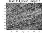
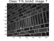
This experiment involves clustering images from the classes “T14_brick1” and “T15_brick2” of the Texture images dataset [34]. Fig. 3 visualizes some example images from these classes.

Figure 3: Example images from classes “T15_brick2” and “T14_brick1” of the Texture dataset. Circles mark detected SIFT keypoints.

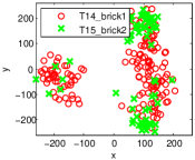
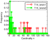
Features are extracted from each image by applying the SIFT algorithm, followed by Principal Component Analysis (PCA) to convert the 128-D SIFT features into 2-D features. Thus each image is compressed into a point pattern of 2-D features. Fig. 4 plots the 2-D features of the images in the Texture images dataset. The clustering algorithm is used to group together point patterns extracted from images of the same class.

(a)

(b)

Figure 4: Extracted data from images of two classes “T15_brick2” and “T14_brick1” of the Texture data. (a) 2-D features (after applying PCA to the SIFT features) of images. (b) Histogram of cardinalities of images.

The AP clustering results for various set distances are shown in Fig. 5. Observe that for this dataset, the OSPA distance achieves a better performance than the Hausdorff and Wasserstein distances.

Figure 5: Performance of AP clustering with various set distances on the Texture image data set (section II-C2).

III Model-based clustering for
point pattern data

In this section, we present generative models for clusters of point pattern data. In particular, the point patterns are assumed to be distributed according a finite mixture of iid cluster random finite set distributions. We then derive an Expectation-Maximization (EM) algorithm to learn the parameters of these models, which are then used to cluster the data.

III-A Random Finite Set

Point patterns can be modeled as random finite sets (RFSs), or simple finite point processes. The likelihood of a point pattern of discrete features is straightforward since this is simply the product of the cardinality distribution and the joint probability of the features given the cardinality. The difficulties arise in continuous feature spaces. In this work, we only consider continuous feature spaces.

Let $\mathcal{F}(\mathcal{X})$ denote the space of finite subsets of a space $\mathcal{X}$. A random finite set (RFS) $X$ of $\mathcal{X}$ is a random variable taking values in $\mathcal{F}(\mathcal{X})$. An RFS $X$ can be completely specified by a discrete (or categorical) distribution that characterizes the cardinality $|X|$, and a family of symmetric joint distributions that characterizes the distribution of the points (or features) of $X$, conditional on the cardinality.

Analogous to random vectors, the probability density of an RFS (if it exists) is essential in the modeling of point pattern data. The probability density $p:\mathcal{F}(\mathcal{X})\rightarrow[0,\infty)$ of an RFS is the Radon-Nikodym derivative of its probability distribution relative to the dominating measure $\mu$, defined for each (measurable) $\mathcal{T}$ $\subseteq$ $\mathcal{F}(\mathcal{X})$, by [24, 26, 36, 37]:

$$\mu(\mathcal{T})=\sum_{m=0}^{\infty}\frac{1}{m!U^{m}}\int\mathbf{1}_{\mathcal{T}}\left(\{x_{1},...,x_{m}\}\right)d\left(x_{1},...,x_{m}\right)$$ (4)

where $U$ is the unit of hyper-volume in $\mathcal{X}$, and $\mathbf{1}_{\mathcal{T}}(\cdot)$ is the indicator function for $\mathcal{T}$. The measure $\mu$ is the unnormalized distribution of a Poisson point process with unit intensity $u=1/U$ when $\mathcal{X}$ is bounded. Note that $\mu$ is unitless and consequently the probability density $p$ is also unitless.

In general the probability density of an RFS, with respect to $\mu$, evaluated at $X=\{x_{1},...,x_{m}\}$ can be written as [38, p. 27] ((Eqs. (1.5), (1.6), and (1.7)), [26]:

$$p(X)=p_{c}(m)\,m!\,U^{m}f_{m}\left(x_{1},...,x_{m}\right),$$ (5)

where $p_{c}(m)=\mbox{Pr}(|X|=m)$ is the cardinality distribution, and $f_{m}\left(x_{1},...,x_{m}\right)$ is a symmetric joint probability density of the points $x_{1},...,x_{m}$ given the cardinality.

Imposing the independence assumption among the features on the model in (5) reduces to the iid-cluster RFS model [25]

$$p(X)=p_{c}(|X|)\,|X|!\,[Up_{f}]^{X}$$ (6)

where $p_{f}$ is a probability density on $\mathcal{X}$, referred to as the feature density, and $h^{X}\triangleq\prod_{x\in X}h(x)$, with $h^{\emptyset}=1$ by convention, is the finite-set exponential notation.

When $p_{c}$ is a Poisson distribution we have the celebrated Poisson point process (aka, Poisson RFS)

$$p(X)=\lambda^{|X|}\,e^{-\lambda}\,[Up_{f}]^{X}$$ (7)

where $\lambda$ is the mean cardinality. The Poisson model is completely determined by the intensity function $u=\lambda p_{f}$ [36, 37]. Note that the Poisson cardinality distribution is described by a single non-negative number $\lambda$, hence there is only one degree of freedom in the choice of cardinality distribution for the Poisson model.

III-B Mixture of iid-cluster RFSs

A mixture of iid-cluster RFSs is a probability density of the form

$$p(X\mid\Theta)=\sum_{k=1}^{N_{\mathrm{comp}}}w_{k}\,p(X\mid\mathscr{C}_{k},\mathscr{F}_{k})$$ (8)

where $k\in\left\{1,...N_{\mathrm{comp}}\right\}$ is the component label, $w_{k}=\mbox{Pr}(C=k)$ is the component weight (the probability of an observation belonging to the $k^{th}$ component), and

$$p(X\mid\mathscr{C}_{k},\mathscr{F}_{k})=p_{c}(|X|\mid\mathscr{C}_{k})\,|X|!\,U^{|X|}\prod_{x\in X}p_{f}(x\mid\mathscr{F}_{k})$$ (9)

is iid-cluster density of the $k^{th}$ component with cardinality distribution parameter $\mathscr{C}_{k}$, and feature distribution parameter $\mathscr{F}_{k}$.

Note that $\Theta=\left\{\left(w_{k},\mathscr{C}_{k},\mathscr{F}_{k}\right):k=1,...,N_{\mathrm{comp}}\right\}$ is the complete collection of parameters of the iid-cluster mixture model. The probability density (8) is a likelihood function for iid point patterns arising from $N_{\mathrm{comp}}$ clusters.

III-C EM clustering using mixture of iid-cluster RFSs

Given a dataset $\mathcal{D}=\left(X_{1},...,X_{N_{\mathrm{data}}}\right)$ where each datum is a point pattern $X_{n}=\left\{x_{n,1},...,x_{n,|X_{n}|}\right\}$. Assume that $\mathcal{D}$ is generated from an underlying iid-cluster RFS mixture model with $N_{\mathrm{comp}}$ components (8) where each component represents a data cluster. The EM clustering for the given data includes two main steps:

1. Model learning: Estimate the parameters of the underlying model using EM method.

2. Cluster assignment: Assign observations to clusters using maximum a posteriori (MAP) estimation.

Input: dataset $\mathcal{D}=\left\{X_{1},...,X_{N_{\mathrm{data}}}\right\}$, no. of components $N_{\mathrm{comp}}$, no. of iterations $N_{\mathrm{iter}}$

Output: parameters $\Theta$ of the iid-cluster RFS mixture model

initialize $\Theta^{(0)}=\left\{\left(w_{k}^{(0)},\mathscr{C}_{k}^{(0)},\mathscr{F}_{k}^{(0)}\right):k=1,...,N_{\mathrm{comp}}\right\}$

for $i=1$ to $N_{\mathrm{iter}}$

/* Compute posteriors */

for $n=1$ to $N_{\mathrm{data}}$

for $k=1$ to $N_{\mathrm{comp}}$

$$p(k\mid X_{n},\Theta^{(i\mbox{-}1)})=\frac{w_{k}^{(i\mbox{-}1)}\,p(X_{n}\mid\mathscr{C}_{k}^{(i\mbox{-}1)},\mathscr{F}_{k}^{(i\mbox{-}1)})}{\sum_{\ell=1}^{N_{\mathrm{comp}}}{\displaystyle w_{\ell}^{(i\mbox{-}1)}\,p(X_{n}\mid\mathscr{C}_{\ell}^{(i\mbox{-}1)},\mathscr{F}_{\ell}^{(i\mbox{-}1)})}}$$ (10)

end

end

for $k=1$ to $N_{\mathrm{comp}}$

/* Update component weights */

$$w_{k}^{(i)}=\frac{1}{N_{\mathrm{data}}}\sum_{n=1}^{N_{\mathrm{data}}}p(k\mid X_{n},\Theta^{(i\mbox{-}1)})\,\,\,\,\,\,\,\,\,\,\,\,\,\,\,\,\,\,\,\,\,\,\,\,\,\,\,\,$$ (11)

/* Update cardinality distribution parameters */

for $m=0$ to $N_{\mathrm{card}}$

$$\,\,\,\,\,\,\,\,\,q_{k,m}^{(i)}=\frac{\sum_{n=1}^{N_{\mathrm{data}}}\delta_{(m\mbox{-}|X_{n}|)}\,p(k\mid X_{n},\Theta^{(i\mbox{-}1)})}{\sum_{\ell=0}^{N_{\mathrm{card}}}\sum_{n=1}^{N_{\mathrm{data}}}\delta_{(\ell\mbox{-}|X_{n}|)}\,p(k\mid X_{n},\Theta^{(i\mbox{-}1)})}$$ (12)

end

/* Update feature density parameters */

$$\,\,\,\,\,\,\,\,\,\boldsymbol{\mu}_{k}^{(i)}= \frac{\sum_{n=1}^{N_{\mathrm{data}}}\left(p(k\mid X_{n},\Theta^{(i\mbox{-}1)})\,\sum_{x\in X_{n}}x\right)}{\sum_{n=1}^{N_{\mathrm{data}}}{\displaystyle|X_{n}|}\,p(k\mid X_{n},\Theta^{(i\mbox{-}1)})}$$ (13)

$$\,\,\,\,\,\,\,\,\,\boldsymbol{\Sigma}_{k}^{(i)}= \frac{\sum_{n=1}^{N_{\mathrm{data}}}{\displaystyle p(k\mid X_{n},\Theta^{(i\mbox{-}1)})}\sum_{x\in X_{n}}\sum_{\ell=1}^{|X_{n}|}\mathbf{K}^{(i)}(x)}{\sum_{n=1}^{N_{\mathrm{data}}}{\displaystyle|X_{n}|\,p(k\mid X_{n},\Theta^{(i\mbox{-}1)})}}$$ (14)

where $\mathbf{K}^{(i)}(x)=\left(x-\boldsymbol{\mu}_{k}^{(i)}\right)\left(x-\boldsymbol{\mu}_{k}^{(i)}\right)^{T}$

end

end

return $\Theta^{(N_{\mathrm{iter}})}$

Algorithm 1 EM algorithm for mixture of iid-cluster RFSs

Model learning step: In this paper, we present EM learning for the iid-cluster mixture model (8) with categorical cardinality distribution and Gaussian feature distribution, i.e., the parameters of the $k^{th}$ component are

$$\mathscr{C}_{k} =\left\{\left(q_{k,0},...,q_{k,N_{\mathrm{card}}}\right):0\leq q_{k,m}\leq 1,\sum_{m=0}^{N_{\mathrm{card}}}q_{k,m}=1\right\}$$

$$\mathscr{F}_{k} =\left\{\left(\boldsymbol{\mu}_{k},\boldsymbol{\Sigma}_{k}\right)\right\}$$

where $N_{\mathrm{card}}$ is the maximum cardinality of point patterns, $\boldsymbol{\mu}_{k},\boldsymbol{\Sigma}_{k}$ are the means and covariances of the Gaussian distributions. The EM algorithm for learning the model parameters $\Theta=\left\{\left(w_{k},\mathscr{C}_{k},\mathscr{F}_{k}\right):k=1,...,N_{\mathrm{comp}}\right\}$ proceeds as shown in Algorithm 1.

In each iteration of Algorithm 1, the parameters are estimated by $\Theta^{(i)}=\mbox{argmax}_{\Theta}Q\left(\Theta,\Theta^{(i-1)}\right)$ [39], where

$$Q\left(\Theta,\Theta^{(i-1)}\right)$$

$$=\sum_{k=1}^{N_{\mathrm{comp}}}{\displaystyle\sum_{n=1}^{N_{\mathrm{data}}}\log}\left(w_{k}\,p(X_{n}\mid\mathscr{C}_{k},\mathscr{F}_{k})\right)\,p(k\mid X_{n},\Theta^{(i\mbox{-}1)})$$ (15)

and $p(X_{n}\mid\mathscr{C}_{k},\mathscr{F}_{k})$, $p(k\mid X_{n},\Theta^{(i\mbox{-}1)})$ are given by (9), (10) respectively.

Cluster assignment step: The cluster label $k_{n}$ of an observation $X_{n}$ can be estimated using MAP estimation:

$$\hat{k}_{n}=\underset{k\in\mathbb{K}}{\mbox{argmax}}p(k\mid X_{n},\Theta),$$ (16)

where $\mathbb{K}=\left\{1,...,N_{\mathrm{comp}}\right\}$, parameters $\Theta$ are learned by Algorithm 1, and $p(k\mid X_{n},\Theta)$ is the posterior probability:

$$p(k\mid X_{n},\Theta)=\frac{w_{k}\,p(X_{n}\mid\mathscr{C}_{k},\mathscr{F}_{k})}{\sum_{\ell=1}^{N_{\mathrm{comp}}}{\displaystyle w_{\ell}\,p(X_{n}\mid\mathscr{C}_{\ell},\mathscr{F}_{\ell})}}.$$ (17)

III-D Numerical experiments

In this section, we evaluate the proposed EM clustering with both simulated and real data. For comparison with AP clustering, we use the same datasets from section II-C. Note that our experiments assume a mixture of Poisson RFSs model.

III-D1 EM clustering with simulated data

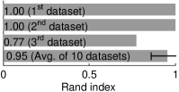
In this experiment we apply EM clustering on the same (simulated) datasets from section II-C1. The performance is shown in Fig. 6. EM clustering performs very well for these datasets with the average Rand index of 0.95.

Figure 6: Performance of the EM clustering on simulated datasets (the same datasets from section II-C1).

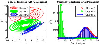
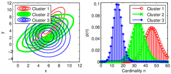
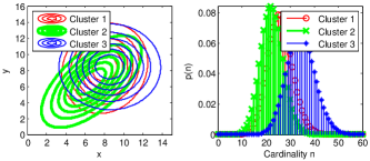
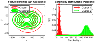
To further investigate performance of the proposed algorithm, we illustrate in Fig. 7 the distributions learned by the EM algorithm for the 3 datasets shown in Fig. 2. Observe that the model-based method has better performance than the non-parametric method when there is little overlap between the feature distributions or cardinality distributions of the data model (e.g., the $1^{st}$ and $2^{nd}$ simulated dataset). However, as expected, if there is significant overlap in both the feature distributions and the cardinality distributions, then model-based clustering performs poorly since there is not enough information to separate the data (e.g., the $3^{rd}$ simulated dataset).

(a) $1^{th}$ dataset

(b) $2^{th}$ dataset

(c) $3^{th}$ dataset

Figure 7: The RFS distributions learned by EM for 3 simulated datasets (corresponding with 3 datasets in Fig. 2). In each subplot, Left: feature distributions, Right: cardinality distributions.

Figure 8: Performance of the EM clustering on the Texture dataset (described in section II-C2). The clustering is evaluated with different number of iterations $N_{\mathrm{iter}}=\{1,...,10\}$.

III-D2 EM clustering with real data

In this experiment, we cluster the Texture dataset (described in section II-C2) using EM clustering with various iterations $N_{\mathrm{iter}}=\{1,...,10\}$. The performance is shown in Fig. 8. The best performance is Rand index of 0.86, which is equal the best performance of AP clustering using OSPA with $c=60$ (Fig. 5). Fig. 9 shows the learned distribution after 10 EM iterations.

Figure 9: The learned RFS distributions for Texture data after 10 EM iterations. Left: feature distributions, Right: cardinality distributions.

IV Conclusion

This paper has detailed a non-parametric approach (based on set distance) and a model-based approach (based on random finite set) to the clustering problem for point pattern data (aka ‘bags’ or multiple instance data). Experiments with both simulated and real data indicate that, in the non-parametric method, the choice of distance has a big influence on the clustering performance. The experiments also indicate that the model-based method has better performance than the non-parametric method when there is little overlap between the feature distributions or cardinality distributions of the data model. However, as expected, if there is significant overlap in both the feature distributions and the cardinality distributions, then model-based clustering performs poorly since there is not enough discriminative information to separate the data.

Future research directions may include developing more complex RFS models such as RFSs with Gaussian mixture feature distribution which can capture better multiple modes feature data (e.g., section II-C2). Another promising development is adapting the proposed clustering algorithms into data stream mining – an emerging research topic dealing with rapidly and continuously generated data such as search or surveillance data [40].

References

- [1] K. P. Murphy, Machine learning: a probabilistic perspective. MIT press, 2012.
- [2] A. K. Jain, M. N. Murty, and P. J. Flynn, “Data clustering: a review,” ACM computing surveys (CSUR), vol. 31, no. 3, pp. 264–323, 1999.
- [3] S. Russell and P. Norvig, Artificial intelligence: A modern approach. Prentice Hall, 2003.
- [4] R. C. Tryon, Cluster analysis: correlation profile and orthometric (factor) analysis for the isolation of unities in mind and personality. Edwards brother, Incorporated, lithoprinters and publishers, 1939.
- [5] D. J. Witherspoon, S. Wooding, A. R. Rogers, E. E. Marchani, W. S. Watkins, M. A. Batzer, and L. B. Jorde, “Genetic similarities within and between human populations,” Genetics, vol. 176, no. 1, pp. 351–359, 2007.
- [6] M.-S. Yang, Y.-J. Hu, K. C.-R. Lin, and C. C.-L. Lin, “Segmentation techniques for tissue differentiation in mri of ophthalmology using fuzzy clustering algorithms,” Magnetic Resonance Imaging, vol. 20, no. 2, pp. 173–179, 2002.
- [7] G. Arimond and A. Elfessi, “A clustering method for categorical data in tourism market segmentation research,” Journal of Travel Research, vol. 39, no. 4, pp. 391–397, 2001.
- [8] N. Mishra, R. Schreiber, I. Stanton, and R. E. Tarjan, “Clustering social networks,” in Algorithms and Models for the Web-Graph. Springer, 2007, pp. 56–67.
- [9] V. Nguyen, A. Martinelli, N. Tomatis, and R. Siegwart, “A comparison of line extraction algorithms using 2d laser rangefinder for indoor mobile robotics,” in Intelligent Robots and Systems, 2005.(IROS 2005). 2005 IEEE/RSJ International Conference on. IEEE, 2005, pp. 1929–1934.
- [10] A. K. Jain, “Data clustering: 50 years beyond k-means,” Pattern recognition letters, vol. 31, no. 8, pp. 651–666, 2010.
- [11] R. Xu and D. Wunsch, “Survey of clustering algorithms,” IEEE Transactions on neural networks, vol. 16, no. 3, pp. 645–678, 2005.
- [12] T. Joachims, “A probabilistic analysis of the rocchio algorithm with tfidf for text categorization.” DTIC Document, Tech. Rep., 1996.
- [13] A. McCallum and K. Nigam, “A comparison of event models for naive Bayes text classification,” in AAAI-98 workshop on learning for text categorization, vol. 752. Citeseer, 1998, pp. 41–48.
- [14] G. Csurka, C. Dance, L. Fan, J. Willamowski, and C. Bray, “Visual categorization with bags of keypoints,” in Workshop on statistical learning in computer vision, ECCV, 2004.
- [15] L. Fei-Fei and P. Perona, “A Bayesian hierarchical model for learning natural scene categories,” in Computer Vision and Pattern Recognition, 2005. CVPR 2005. IEEE Computer Society Conference on, vol. 2. IEEE, 2005, pp. 524–531.
- [16] S. Guha, R. Rastogi, and K. Shim, “Rock: A robust clustering algorithm for categorical attributes,” in Data Engineering, 1999. Proceedings., 15th International Conference on. IEEE, 1999, pp. 512–521.
- [17] Y. Yang, X. Guan, and J. You, “Clope: a fast and effective clustering algorithm for transactional data,” in Proceedings of the eighth ACM SIGKDD international conference on Knowledge discovery and data mining. ACM, 2002, pp. 682–687.
- [18] C.-H. Yun, K.-T. Chuang, and M.-S. Chen, “An efficient clustering algorithm for market basket data based on small large ratios,” in Computer Software and Applications Conference, 2001. COMPSAC 2001. 25th Annual International. IEEE, 2001, pp. 505–510.
- [19] I. V. Cadez, S. Gaffney, and P. Smyth, “A general probabilistic framework for clustering individuals and objects,” in Proceedings of the sixth ACM SIGKDD international conference on Knowledge discovery and data mining. ACM, 2000, pp. 140–149.
- [20] T. G. Dietterich, R. H. Lathrop, and T. Lozano-Pérez, “Solving the multiple instance problem with axis-parallel rectangles,” Artificial intelligence, vol. 89, no. 1, pp. 31–71, 1997.
- [21] F. Minhas and A. Ben-Hur, “Multiple instance learning of calmodulin binding sites,” Bioinformatics (Oxford, England), vol. 28, no. 18, pp. i416–i422, 2012.
- [22] J. Amores, “Multiple instance classification: Review, taxonomy and comparative study,” Artificial Intelligence, vol. 201, pp. 81–105, 2013.
- [23] J. Foulds and E. Frank, “A review of multi-instance learning assumptions,” The Knowledge Engineering Review, vol. 25, no. 01, pp. 1–25, 2010.
- [24] D. Stoyan, W. S. Kendall, and J. Mecke, Stochastic geometry and its applications. John Wiley & Sons, 1995.
- [25] D. J. Daley and D. Vere-Jones, An introduction to the theory of point processes. Springer, 1988, vol. 2.
- [26] J. Moller and R. P. Waagepetersen, Statistical inference and simulation for spatial point processes. Chapman & Hall CRC, 2003.
- [27] M.-L. Zhang and Z.-H. Zhou, “Multi-instance clustering with applications to multi-instance prediction,” Applied Intelligence, vol. 31, no. 1, pp. 47–68, 2009.
- [28] D. Zhang, F. Wang, L. Si, and T. Li, “M3ic: Maximum margin multiple instance clustering.” in IJCAI, vol. 9, 2009, pp. 1339–1344.
- [29] B. J. Frey and D. Dueck, “Clustering by passing messages between data points,” Science, vol. 315, no. 5814, pp. 972–976, 2007.
- [30] A. P. Dempster, N. M. Laird, and D. B. Rubin, “Maximum likelihood from incomplete data via the em algorithm,” Journal of the Royal Statistical Society. Series B (Methodological), pp. 1–38, 1977.
- [31] D. Schuhmacher, B.-T. Vo, and B.-N. Vo, “A consistent metric for performance evaluation of multi-object filters,” Signal Processing, IEEE Transactions on, vol. 56, no. 8, pp. 3447–3457, 2008.
- [32] J. R. Hoffman and R. P. Mahler, “Multitarget miss distance via optimal assignment,” Systems, Man and Cybernetics, Part A: Systems and Humans, IEEE Transactions on, vol. 34, no. 3, pp. 327–336, 2004.
- [33] C. D. Manning, P. Raghavan, and H. Schütze, Introduction to information retrieval. Cambridge university press Cambridge, 2008, vol. 1.
- [34] S. Lazebnik, C. Schmid, and J. Ponce, “A sparse texture representation using local affine regions,” Pattern Analysis and Machine Intelligence, IEEE Transactions on, vol. 27, no. 8, pp. 1265–1278, 2005.
- [35] A. Vedaldi and B. Fulkerson, “Vlfeat: An open and portable library of computer vision algorithms,” http://www.vlfeat.org/, 2008.
- [36] B.-N. Vo, S. Singh, and A. Doucet, “Sequential monte carlo methods for multitarget filtering with random finite sets,” Aerospace and Electronic Systems, IEEE Transactions on, vol. 41, no. 4, pp. 1224–1245, 2005.
- [37] H. G. Hoang, B.-N. Vo, B.-T. Vo, and R. Mahler, “The Cauchy-Schwarz divergence for Poisson point processes,” IEEE Trans. Inf. Theory, vol. 61, no. 8, pp. 4475–4485, 2015.
- [38] M. van Lieshout, Markov point processes and their applications. Imperial College Press, 2000.
- [39] J. A. Bilmes, “A gentle tutorial of the em algorithm and its application to parameter estimation for gaussian mixture and hidden markov models,” International Computer Science Institute, vol. 4, no. 510, p. 126, 1998.
- [40] H.-L. Nguyen, Y.-K. Woon, and W.-K. Ng, “A survey on data stream clustering and classification,” Knowledge and information systems, vol. 45, no. 3, pp. 535–569, 2015.