Comparative Study of CNN and RNN for Natural Language Processing
Abstract
Deep neural networks (DNNs) have revolutionized the field of natural language processing (NLP). Convolutional Neural Network (CNN) and Recurrent Neural Network (RNN), the two main types of DNN architectures, are widely explored to handle various NLP tasks. CNN is supposed to be good at extracting position-invariant features and RNN at modeling units in sequence. The state-of-the-art on many NLP tasks often switches due to the battle of CNNs and RNNs. This work is the first systematic comparison of CNN and RNN on a wide range of representative NLP tasks, aiming to give basic guidance for DNN selection.
1 Introduction
Natural language processing (NLP) has benefited greatly from the resurgence of deep neural networks (DNNs), due to their high performance with less need of engineered features. There are two main DNN architectures: convolutional neural network (CNN) LeCun et al. (1998) and recurrent neural network (RNN) Elman (1990). Gating mechanisms have been developed to alleviate some limitations of the basic RNN, resulting in two prevailing RNN types: long short-term memory (LSTM) Hochreiter and Schmidhuber (1997) and gated recurrent unit (GRU) Cho et al. (2014).
Generally speaking, CNNs are hierarchical and RNNs sequential architectures. How should we choose between them for processing language? Based on the characterization “hierarchical (CNN) vs. sequential (RNN)”, it is tempting to choose a CNN for classification tasks like sentiment classification since sentiment is usually determined by some key phrases; and to choose RNNs for a sequence modeling task like language modeling as it requires flexible modeling of context dependencies. But current NLP literature does not support such a clear conclusion. For example, RNNs perform well on document-level sentiment classification Tang et al. (2015); and Dauphin et al. (2016) recently showed that gated CNNs outperform LSTMs on language modeling tasks, even though LSTMs had long been seen as better suited. In summary, there is no consensus on DNN selection for any particular NLP problem.
This work compares CNNs, GRUs and LSTMs systematically on a broad array of NLP tasks: sentiment/relation classification, textual entailment, answer selection, question-relation matching in Freebase, Freebase path query answering and part-of-speech tagging.
Our experiments support two key findings. (i) CNNs and RNNs provide complementary information for text classification tasks. Which architecture performs better depends on how important it is to semantically understand the whole sequence. (ii) Learning rate changes performance relatively smoothly, while changes to hidden size and batch size result in large fluctuations.
2 Related Work
To our knowledge, there has been no systematic comparison of CNN and RNN on a large array of NLP tasks.
Vu et al. (2016) investigate CNN and basic RNN (i.e., no gating mechanisms) for relation classification. They report higher performance of CNN than RNN and give evidence that CNN and RNN provide complementary information: while the RNN computes a weighted combination of all words in the sentence, the CNN extracts the most informative ngrams for the relation and only considers their resulting activations. Both Wen et al. (2016) and Adel and Schütze (2017) support CNN over GRU/LSTM for classification of long sentences. In addition, Yin et al. (2016) achieve better performance of attention-based CNN than attention-based LSTM for answer selection. Dauphin et al. (2016) further argue that a fine-tuned gated CNN can also model long-context dependency, getting new state-of-the-art in language modeling above all RNN competitors
3 Models
This section gives a brief introduction of CNN, GRU and LSTM.
3.1 Convolutional Neural Network (CNN)
Input Layer
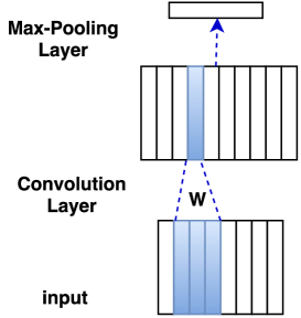
Sequence contains entries. Each entry is represented by a -dimensional dense vector; thus the input is represented as a feature map of dimensionality . Figure 1(a) shows the input layer as the lower rectangle with multiple columns.
Convolution Layer
is used for representation learning from sliding -grams. For an input sequence with entries: , let vector be the concatenated embeddings of entries where is the filter width and . Embeddings for , or , are zero padded. We then generate the representation for the -gram using the convolution weights :
| (1) |
where bias .
Maxpooling
All -gram representations are used to generate the representation of input sequence by maxpooling: ().
3.2 Gated Recurrent Unit (GRU)
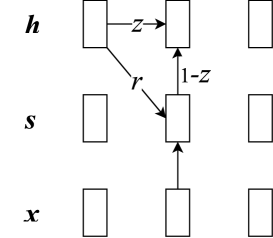
GRU, as shown in Figure 1(b), models text as follows:
| (2) | |||||
| (3) | |||||
| (4) | |||||
| (5) |
represents the token in at position , is the hidden state at , supposed to encode the history , , . and are two gates. All , are parameters.
3.3 Long Short-Time Memory (LSTM)
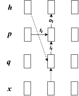
LSTM is denoted in Figure 1(c). It models the word sequence as follows:
| (6) | |||||
| (7) | |||||
| (8) | |||||
| (9) | |||||
| (10) | |||||
| (11) |
LSTM has three gates: input gate , forget gate and output gate . All gates are generated by a sigmoid function over the ensemble of input and the preceding hidden state . In order to generate the hidden state at current step , it first generates a temporary result by a tanh non-linearity over the ensemble of input and the preceding hidden state , then combines this temporary result with history by input gate and forget gate respectively to get an updated history , finally uses output gate over this updated history to get the final hidden state .
4 Experiments
| performance | lr | hidden | batch | sentLen | filter_size | margin | |||
|---|---|---|---|---|---|---|---|---|---|
| TextC | SentiC (acc) | CNN | 82.38 | 0.2 | 20 | 5 | 60 | 3 | – |
| GRU | 86.32 | 0.1 | 30 | 50 | 60 | – | – | ||
| LSTM | 84.51 | 0.2 | 20 | 40 | 60 | – | – | ||
| RC (F1) | CNN | 68.02 | 0.12 | 70 | 10 | 20 | 3 | – | |
| GRU | 68.56 | 0.12 | 80 | 100 | 20 | – | – | ||
| LSTM | 66.45 | 0.1 | 80 | 20 | 20 | – | – | ||
| SemMatch | TE (acc) | CNN | 77.13 | 0.1 | 70 | 50 | 50 | 3 | – |
| GRU | 78.78 | 0.1 | 50 | 80 | 65 | – | – | ||
| LSTM | 77.85 | 0.1 | 80 | 50 | 50 | – | – | ||
| AS (MAP & MRR) | CNN | (63.69,65.01) | 0.01 | 30 | 60 | 40 | 3 | 0.3 | |
| GRU | (62.58,63.59) | 0.1 | 80 | 150 | 40 | – | 0.3 | ||
| LSTM | (62.00,63.26) | 0.1 | 60 | 150 | 45 | – | 0.1 | ||
| QRM (acc) | CNN | 71.50 | 0.125 | 400 | 50 | 17 | 5 | 0.01 | |
| GRU | 69.80 | 1.0 | 400 | 50 | 17 | - | 0.01 | ||
| LSTM | 71.44 | 1.0 | 200 | 50 | 17 | - | 0.01 | ||
| SeqOrder | PQA (hit@10) | CNN | 54.42 | 0.01 | 250 | 50 | 5 | 3 | 0.4 |
| GRU | 55.67 | 0.1 | 250 | 50 | 5 | – | 0.3 | ||
| LSTM | 55.39 | 0.1 | 300 | 50 | 5 | – | 0.3 | ||
| ContextDep | POS tagging (acc) | CNN | 94.18 | 0.1 | 100 | 10 | 60 | 5 | – |
| GRU | 93.15 | 0.1 | 50 | 50 | 60 | – | – | ||
| LSTM | 93.18 | 0.1 | 200 | 70 | 60 | – | – | ||
| Bi-GRU | 94.26 | 0.1 | 50 | 50 | 60 | – | – | ||
| Bi-LSTM | 94.35 | 0.1 | 150 | 5 | 60 | – | – |
| Gold | CNN | GRU | examples |
|---|---|---|---|
| T | F | T | It ’s a movie – and an album – you wo n’t want to miss |
| F | T | F | These are names to remember , in order to avoid them in the future |
| F | F | T | In the second half of the film , Frei ’s control loosens in direct proportion to the |
| amount of screen time he gives nachtwey for self-analysis | |||
| \hdashlineT | T | F | The result is mesmerizing – filled with menace and squalor |
 |
 |
 |
 |
 |
 |
 |
 |
4.1 Tasks
Sentiment Classification (SentiC) on Stanford Sentiment Treebank (SST) Socher et al. (2013). This dataset predicts the sentiment (positive or negative) of movie reviews. We use the given split of 6920 train, 872 dev and 1821 test sentences. As in Kalchbrenner et al. (2014); Le and Mikolov (2014), we treat labeled phrases that occur as subparts of training sentences as independent training instances. Measure: accuracy.
Relation Classification (RC) on SemEval 2010 task 8 Hendrickx et al. (2009). It consists of sentences which have been manually labeled with 19 relations (18 directed relations and Other), 8000 sentences in train and 2717 in test. As there is no dev set, we use 1500 training examples as dev, similar to Vu et al. (2016). Measure: F1.
Textual Entailment (TE) on Stanford Natural Language Inference (SNLI) Bowman et al. (2015). SNLI contains premise-hypothesis pairs, labeled with a relation (entailment, contradiction, neutral). After removing unlabeled pairs, we end up having 549,367 pairs for train, 9,842 for dev and 9,824 for test. Measure: accuracy.
Answer Selection (AS) on WikiQA Yang et al. (2015), an open domain question-answer dataset. We use the subtask that assumes that there is at least one correct answer for a question. The corresponding dataset consists of 20,360 question-candidate pairs in train, 1,130 in dev and 2,352 in test where we adopt the standard setup of only considering questions with correct answers in test. The task is to choose the correct answer(s) from some candidates for a question. Measures: MAP and MRR.
Question Relation Match (QRM). We utilize WebQSP Yih et al. (2016) dataset to create a large-scale relation detection task, benefitting from the availability of labeled semantic parses of questions. For each question, we (i) select the topic entity from the parse; (ii) select all the relations/relation chains (length 2) connecting to the topic entity; and (iii) set the relations/relation-chains in the labeled parse as positive and all the others as negative. Following Yih et al. (2016) and Xu et al. (2016), we formulate this task as a sequence matching problem. Ranking-loss is used for training. Measure: accuracy.
Path Query Answering (PQA) on the path query dataset released by Guu et al. (2015). It contains KB paths like , where head entity and relation sequence are encoded to predict the tail entity . There are 6,266,058/27,163/109,557 paths in train/dev/test, respectively. Measure: hit@10.
Part-of-Speech Tagging on WSJ. We use the setup of Blitzer et al. (2006); Petrov and McDonald (2012): sections 2-21 are train, section 22 is dev and section 23 is test. Measure: accuracy.
We organize above tasks in four categories. (i) TextC. Text classification, including SentiC and RC. (ii) SemMatch including TE, AS and QRM. (iii) SeqOrder. Sequence order, i.e., PQA. (iv) ContextDep. Context dependency, i.e., POS tagging. By investigating these four categories, we aim to discover some basic principles involved in utilizing CNNs / RNNs.
4.2 Experimental Setup
To fairly study the encoding capability of different basic DNNs, our experiments have the following design. (i) Always train from scratch, no extra knowledge, e.g., no pretrained word embeddings. (ii) Always train using a basic setup without complex tricks such as batch normalization. (iii) Search for optimal hyperparameters for each task and each model separately, so that all results are based on optimal hyperparameters. (iv) Investigate the basic architecture and utilization of each model: CNN consists of a convolution layer and a max-pooling layer; GRU and LSTM model the input from left to right and always use the last hidden state as the final representation of the input. An exception is for POS tagging, we also report bi-directional RNNs as this can make sure each word’s representation can encode the word’s context of both sides, like the CNN does.
Hyperparameters are tuned on dev: hidden size, minibatch size, learning rate, maximal sentence length, filter size (for CNN only) and margin in ranking loss in AS, QRM and PQA tasks.
4.3 Results & Analysis
Table 1 shows experimental results for all tasks and models and corresponding hyperparameters. For TextC, GRU performs best on SentiC and comparably with CNN in RC. For SemMatch, CNN performs best on AS and QRM while GRU (and also LSTM) outperforms CNN on TE. For SeqOrder (PQA), both GRU and LSTM outperform CNN. For ContextDep (POS tagging), CNN outperforms one-directional RNNs, but lags behind bi-directional RNNs.
The results for SeqOrder and ContextDep are as expected: RNNs are well suited to encode order information (for PQA) and long-range context dependency (for POS tagging). But for the other two categories, TextC and SemMatch, some unexpected observations appear. CNNs are considered good at extracting local and position-invariant features and therefore should perform well on TextC; but in our experiments they are outperformed by RNNs, especially in SentiC. How can this be explained? RNNs can encode the structure-dependent semantics of the whole input, but how likely is this helpful for TextC tasks that mostly depend on a few local regions? To investigate the unexpected observations, we do some error analysis on SentiC.
Qualitative analysis
Table 2 shows examples (1) – (4) in which CNN predicts correctly while GRU predicts falsely or vice versa. We find that GRU is better when sentiment is determined by the entire sentence or a long-range semantic dependency – rather than some local key-phrases – is involved. Example (1) contains the phrases “won’t” and “miss” that usually appear with negative sentiment, but the whole sentence describes a positive sentiment; thus, an architecture like GRU is needed that handles long sequences correctly. On the other hand, modeling the whole sentence sometimes is a burden – neglecting the key parts. The GRU encodes the entire word sequence of the long example (3), making it hard for the negative keyphrase “loosens” to play a main role in the final representation. The first part of example (4) seems positive while the second part seems negative. As GRU chooses the last hidden state to represent the sentence, this might result in the wrong prediction.
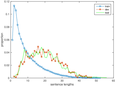
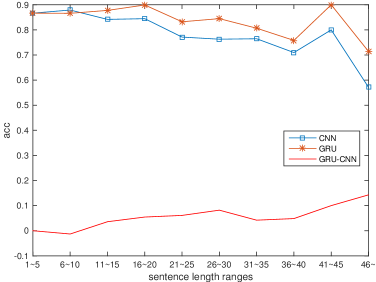
Studying acc vs sentence length can also support this. Figure 2 (left) shows sentence lengths in SST are mostly short in train while close to normal distribution around 20 in dev and test. Figure 2 (right) depicts the accuracies w.r.t length ranges. We found that GRU and CNN are comparable when lengths are small, e.g., 10, then GRU gets increasing advantage over CNN when meet longer sentences. Error analysis shows that long sentences in SST mostly consist of clauses of inverse semantic such as “this version is not classic like its predecessor, but its pleasures are still plentiful”. This kind of clause often include a local strong indicator for one sentiment polarity, like “is not” above, but the successful classification relies on the comprehension of the whole clause.
Hence, which DNN type performs better in text classification task depends on how often the comprehension of global/long-range semantics is required.
This can also explain the phenomenon in SemMatch – GRU/LSTM surpass CNN in TE while CNN dominates in AS, as textual entailment relies on the comprehension of the whole sentence Bowman et al. (2015), question-answer in AS instead can be effectively identified by key-phrase matching Yin et al. (2016).
Sensitivity to hyperparameters
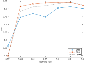
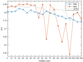
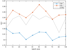
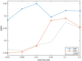
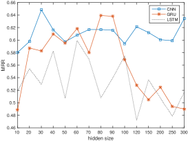
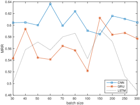
We next check how stable the performance of CNN and GRU are when hyperparameter values are varied. Figure 3 shows the performance of CNN, GRU and LSTM for different learning rates, hidden sizes and batch sizes. All models are relativly smooth with respect to learning rate changes. In contrast, variation in hidden size and batch size cause large oscillations. Nevertheless, we still can observe that CNN curve is mostly below the curves of GRU and LSTM in SentiC task, contrarily located at the higher place in AS task.
5 Conclusions
This work compared the three most widely used DNNs – CNN, GRU and LSTM – in representative sample of NLP tasks. We found that RNNs perform well and robust in a broad range of tasks except when the task is essentially a keyphrase recognition task as in some sentiment detection and question-answer matching settings. In addition, hidden size and batch size can make DNN performance vary dramatically. This suggests that optimization of these two parameters is crucial to good performance of both CNNs and RNNs.
References
- Adel and Schütze (2017) Heike Adel and Hinrich Schütze. 2017. Exploring different dimensions of attention for uncertainty detection. In Proceedings of EACL.
- Arkhipenko et al. (2016) K. Arkhipenko, I. Kozlov, J. Trofimovich, K. Skorniakov, A. Gomzin, and D. Turdakov. 2016. Comparison of neural network architectures for sentiment analysis of russian tweets. In Proceedings of “Dialogue 2016”.
- Blitzer et al. (2006) John Blitzer, Ryan McDonald, and Fernando Pereira. 2006. Domain adaptation with structural correspondence learning. In Proceedings of EMNLP. pages 120–128.
- Bowman et al. (2015) Samuel R Bowman, Gabor Angeli, Christopher Potts, and Christopher D Manning. 2015. A large annotated corpus for learning natural language inference. In Proceedings of EMNLP. pages 632–642.
- Cho et al. (2014) Kyunghyun Cho, Bart van Merriënboer, Dzmitry Bahdanau, and Yoshua Bengio. 2014. On the properties of neural machine translation: Encoder-decoder approaches. Eighth Workshop on Syntax, Semantics and Structure in Statistical Translation .
- Chung et al. (2014) Junyoung Chung, Caglar Gulcehre, KyungHyun Cho, and Yoshua Bengio. 2014. Empirical evaluation of gated recurrent neural networks on sequence modeling. arXiv preprint arXiv:1412.3555 .
- Dauphin et al. (2016) Yann N Dauphin, Angela Fan, Michael Auli, and David Grangier. 2016. Language modeling with gated convolutional networks. arXiv preprint arXiv:1612.08083 .
- Elman (1990) Jeffrey L. Elman. 1990. Finding structure in time. Cognitive Science 14(2):179–211.
- Guu et al. (2015) Kelvin Guu, John Miller, and Percy Liang. 2015. Traversing knowledge graphs in vector space. In Proceedings of EMNLP. pages 318–327.
- Hendrickx et al. (2009) Iris Hendrickx, Su Nam Kim, Zornitsa Kozareva, Preslav Nakov, Diarmuid Ó Séaghdha, Sebastian Padó, Marco Pennacchiotti, Lorenza Romano, and Stan Szpakowicz. 2009. Semeval-2010 task 8: Multi-way classification of semantic relations between pairs of nominals. In Proceedings of SemEval. pages 94–99.
- Hochreiter and Schmidhuber (1997) Sepp Hochreiter and Jürgen Schmidhuber. 1997. Long short-term memory. Neural computation 9(8):1735–1780.
- Jozefowicz et al. (2015) Rafal Jozefowicz, Wojciech Zaremba, and Ilya Sutskever. 2015. An empirical exploration of recurrent network architectures. In Proceedings of ICML. pages 2342–2350.
- Kalchbrenner et al. (2014) Nal Kalchbrenner, Edward Grefenstette, and Phil Blunsom. 2014. A convolutional neural network for modelling sentences. In Proceedings of ACL.
- Le and Mikolov (2014) Quoc V Le and Tomas Mikolov. 2014. Distributed representations of sentences and documents. In Proceedings of ICML. pages 1188–1196.
- LeCun et al. (1998) Yann LeCun, Léon Bottou, Yoshua Bengio, and Patrick Haffner. 1998. Gradient-based learning applied to document recognition. Proceedings of the IEEE 86(11):2278–2324.
- Mikolov et al. (2013) Tomas Mikolov, Ilya Sutskever, Kai Chen, Gregory S. Corrado, and Jeffrey Dean. 2013. Distributed representations of words and phrases and their compositionality. In Proceedings of NIPS. pages 3111–3119.
- Petrov and McDonald (2012) Slav Petrov and Ryan McDonald. 2012. Overview of the 2012 shared task on parsing the web. In Notes of the First Workshop on Syntactic Analysis of Non-Canonical Language (SANCL). volume 59.
- Socher et al. (2013) Richard Socher, Alex Perelygin, Jean Y Wu, Jason Chuang, Christopher D Manning, Andrew Y Ng, and Christopher Potts. 2013. Recursive deep models for semantic compositionality over a sentiment treebank. In Proceedings EMNLP. volume 1631, page 1642.
- Tang et al. (2015) Duyu Tang, Bing Qin, and Ting Liu. 2015. Document modeling with gated recurrent neural network for sentiment classification. In Proceedings of EMNLP. pages 1422–1432.
- Vu et al. (2016) Ngoc Thang Vu, Heike Adel, Pankaj Gupta, and Hinrich Schütze. 2016. Combining recurrent and convolutional neural networks for relation classification. In Proceedings of NAACL HLT. pages 534–539.
- Wen et al. (2016) Ying Wen, Weinan Zhang, Rui Luo, and Jun Wang. 2016. Learning text representation using recurrent convolutional neural network with highway layers. SIGIR Workshop on Neural Information Retrieval .
- Xu et al. (2016) Kun Xu, Yansong Feng, Siva Reddy, Songfang Huang, and Dongyan Zhao. 2016. Enhancing freebase question answering using textual evidence. CoRR abs/1603.00957.
- Yang et al. (2015) Yi Yang, Wen-tau Yih, and Christopher Meek. 2015. Wikiqa: A challenge dataset for open-domain question answering. In Proceedings of EMNLP. pages 2013–2018.
- Yih et al. (2016) Wen-tau Yih, Matthew Richardson, Chris Meek, Ming-Wei Chang, and Jina Suh. 2016. The value of semantic parse labeling for knowledge base question answering. In Proceedings of ACL. pages 201–206.
- Yin et al. (2016) Wenpeng Yin, Hinrich Schütze, Bing Xiang, and Bowen Zhou. 2016. ABCNN: attention-based convolutional neural network for modeling sentence pairs. TACL 4:259–272.