Large-scale Image Geo-Localization
Using Dominant Sets
Abstract
This paper presents a new approach for the challenging problem of geo-localization using image matching in a structured database of city-wide reference images with known GPS coordinates. We cast the geo-localization as a clustering problem of local image features. Akin to existing approaches to the problem, our framework builds on low-level features which allow local matching between images. For each local feature in the query image, we find its approximate nearest neighbors in the reference set. Next, we cluster the features from reference images using Dominant Set clustering, which affords several advantages over existing approaches. First, it permits variable number of nodes in the cluster, which we use to dynamically select the number of nearest neighbors for each query feature based on its discrimination value. Second, this approach is several orders of magnitude faster than existing approaches. Thus, we obtain multiple clusters (different local maximizers) and obtain a robust final solution to the problem using multiple weak solutions through constrained Dominant Set clustering on global image features, where we enforce the constraint that the query image must be included in the cluster. This second level of clustering also bypasses heuristic approaches to voting and selecting the reference image that matches to the query. We evaluate the proposed framework on an existing dataset of 102k street view images as well as a new larger dataset of 300k images, and show that it outperforms the state-of-the-art by 20% and 7%, respectively, on the two datasets.
Index Terms:
Geo-localization, Dominant Set Clustering, Multiple Nearest Neighbor Feature Matching, Constrained Dominant Set1 Introduction
Image geo-localization, the problem of determining the location of an image using just the visual information, is remarkably difficult. Nonetheless, images often contain useful visual and contextual informative cues which allow us to determine the location of an image with variable confidence. The foremost of these cues are landmarks, architectural details, building textures and colors, in addition to road markings and surrounding vegetation.
Recently, the geo-localization through image-matching approach was proposed in [1, 2]. In [1], the authors find the first nearest neighbor (NN) for each local feature in the query image, prune outliers and use a heuristic voting scheme for selecting the matched reference image. The follow-up work [2] relaxes the restriction of using only the first NN and proposed Generalized Minimum Clique Problem (GMCP) formulation for solving this problem. However, GMCP formulation can only handle a fixed number of nearest neighbors for each query feature. The authors used 5 NN, and found that increasing the number of NN drops the performance. Additionally, the GMCP formulation selects exactly one NN per query feature. This makes the optimization sensitive to outliers, since it is possible that none of the 5 NN is correct. Once the best NN is selected for each query feature, a very simple voting scheme is used to select the best match. Effectively, each query feature votes for a single reference image, from which the NN was selected for that particular query feature. This often results in identical number of votes for several images from the reference set. Then, both [1, 2] proceed with randomly selecting one reference image as the correct match to infer GPS location of the query image. Furthermore, the GMCP is a binary-variable NP-hard problem, and due to the high computational cost, only a single local minima solution is computed in [2].
In this paper, we propose an approach to image geo-localization by robustly finding a matching reference image to a given query image. This is done by finding correspondences between local features of the query and reference images. We first introduce automatic NN selection into our framework, by exploiting the discriminative power of each NN feature and employing different number of NN for each query feature. That is, if the distance between query and reference NNs is similar, then we use several NNs since they are ambiguous, and the optimization is afforded with more choices to select the correct match. On the other hand, if a query feature has very few low-distance reference NNs, then we use fewer NNs to save the computation cost. Thus, for some cases we use fewer NNs, while for others we use more requiring on the average approximately the same amount of computation power, but improving the performance, nonetheless. This also bypasses the manual tuning of the number of NNs to be considered, which can vary between datasets and is not straightforward.
Our approach to image geo-localization is based on Dominant Set clustering (DSC) - a well-known generalization of maximal clique problem to edge-weighted graphs- where the goal is to extract the most compact and coherent set. It’s intriguing connections to evolutionary game theory allow us to use efficient game dynamics, such as replicator dynamics and infection-immunization dynamics (InImDyn). InImDyn has been shown to have a linear time/space complexity for solving standard quadratic programs (StQPs), programs which deal with finding the extrema of a quadratic polynomial over the standard simplex [3, 4]. The proposed approach is on average 200 times faster and yields an improvement of 20% in the accuracy of geo-localization compared to [1, 2]. This is made possible, in addition to the dynamics, through the flexibility inherent in DSC, which unlike the GMCP formulation avoids any hard constraints on memberships. This naturally handles outliers, since their membership score is lower compared to inliers present in the cluster. Furthermore, our solution uses a linear relaxation to the binary variables, which in the absence of hard constraints is solved through an iterative algorithm resulting in massive speed up.
Since the dynamics and linear relaxation of binary variables allow our method to be extremely fast, we run it multiple times to obtain several local maxima as solutions. Next, we use a query-based variation of DSC to combine those solutions to obtain a final robust solution. The query-based DSC uses the soft-constraint that the query, or a group of queries, must always become part of the cluster, thus ensuring their membership in the solution. We use a fusion of several global features to compute the cost between query and reference images selected from the previous step. The members of the cluster from the reference set are used to find the geo-location of the query image. Note that, the GPS location of matching reference image is also used as a cost in addition to visual features to ensure both visual similarity and geographical proximity.
GPS tagged reference image databases collected from user uploaded images on Flickr have been typically used for the geo-localization task. The query images in our experiments have been collected from Flickr, however, the reference images were collected from Google Street View. The data collected through Flickr and Google Street View differ in several important aspects: the images downloaded from Flickr are often redundant and repetitive, where images of a particular building, landmark or street are captured multiple times by different users. Typically, popular or tourist spots have relatively more images in testing and reference sets compared to less interesting parts of the urban environment. An important constraint during evaluation is that the distribution of testing images should be similar to that of reference images. On the contrary, Google Street View reference data used in this paper contains only a single sample of each location of the city. However, Street View does provide spherical panoramic views, , approximately 12 meters apart, of most streets and roads. Thus, the images are uniformly distributed over different locations, independent of their popularity. The comprehensiveness of the data ensures that a correct match exists; nonetheless, at the same time, the sparsity or uniform distribution of the data makes geo-localization difficult, since every location is captured in only few of the reference images. The difficulty is compounded by the distorted, low-quality nature of the images as well.
The main contributions of this paper are summarized as follows:
-
•
We present a robust and computationally efficient approach for the problem of large-scale image geo-localization by locating images in a structured database of city-wide reference images with known GPS coordinates.
-
•
We formulate geo-localization problem in terms of a more generalized form of dominant sets framework which incorporates weights from the nodes in addition to edges.
-
•
We take a two-step approach to solve the problem. The first step uses local features to find putative set of reference images (and is therefore faster), whereas the second step uses global features and a constrained variation of dominant sets to refine results from the first step, thereby, significantly boosting the geo-localization performance.
-
•
We have collected new and more challenging high resolution reference dataset (WorldCities dataset) of 300K Google street view images.
The rest of the paper is structured as follows. We present literature relevant to our problem in Sec. 2, followed by technical details of the proposed approach in Sec. 3, while constrained dominant set based post processing step is discussed in Sec. 4. This is followed by dataset description in section 5.1. Finally, we provide results of our extensive evaluation in Sec. 5 and conclude in Sec. 6.
2 Related Work
The computer vision literature on the problem of geo-localization can be divided into three categories depending on the scale of the datasets used: landmarks or buildings [5, 6, 7, 8], city-scale including streetview data [9], and worldwide [10, 11, 12]. Landmark recognition is typically formulated as an image retrieval problem [5, 7, 8, 13, 14]. For geo-localization of landmarks and buildings, Crandall et al. [15] perform structural analysis in the form of spatial distribution of millions of geo-tagged photos. This is used in conjunction with visual and meta data from images to geo-locate them. The datasets for this category contain many images near prominent landmarks or images. Therefore, in many works [5, 7], similar looking images belonging to same landmarks are often grouped before geo-localization is undertaken.
For citywide geo-localization of query images, Zamir and Shah [1] performed matching using SIFT features, where each feature votes for a reference image. The vote map is then smoothed geo-spatially and the peak in the vote map is selected as the location of the query image. They also compute ’confidence of localization’ using the Kurtosis measure as it quantifies the peakiness of vote map distribution. The extension of this work in [2] formulates the geo-localization as a clique-finding problem where the authors relax the constraint of using only one nearest neighbor per query feature. The best match for each query feature is then solved using Generalized Minimum Clique Graphs, so that a simultaneous solution is obtained for all query features in contrast to their previous work [1]. In similar vein, Schindler et al. [16] used a dataset of 30,000 images corresponding to 20 kilometers of street-side data captured through a vehicle using vocabulary tree. Sattler et al. [17] investigated ways to explicitly handle geometric bursts by analyzing the geometric relations between the different database images retrieved by a query. Arandjelovic´ et al. [18] developed a convolutional neural network architecture for place recognition that aggregates mid-level (conv5) convolutional features extracted from the entire image into a compact single vector representation amenable to efficient indexing. Torii et al. [19] exploited repetitive structure for visual place recognition, by robustly detecting repeated image structures and a simple modification of weights in the bag-of-visual-word model. Zeisl et al. [20] proposed a voting-based pose estimation strategy that exhibits linear complexity in the number of matches and thus facilitates to consider much more matches.
For geo-localization at the global scale, Hays and Efros [10] were the first to extract coarse geographical location of query images using Flickr collected across the world. Recently, Weyand et al. [12] pose the problem of geo-locating images in terms of classification by subdividing the surface of the earth into thousands of multi-scale geographic cells, and train a deep network using millions of geo-tagged images. In the regions where the coverage of photos is dense, structure-from-motion reconstruction is used for matching query images [21, 22, 23, 24]. Since the difficulty of the problem increases as we move from landmarks to city-scale and finally to worldwide, the performance also drops. There are many interesting variations to the geo-localization problem as well. Sequential information such as chronological order of photos was used by [25] to geo-locate photos. Similarly, there are methods to find trajectory of a moving camera by geo-locating video frames using Bayesian Smoothing [26] or geometric constraints [27]. Chen and Grauman [28] present Hidden Markov Model approach to match sets of images with sets in the database for location estimation. Lin et al. [29] use aerial imagery in conjunction with ground images for geo-localization. Others [30, 31] approach the problem by matching ground images against a database of aerial images. Jacob et al. [32] geo-localize a webcam by correlating its video-stream with satellite weather maps over the same time period. Skyline2GPS [33] uses street view data and segments the skyline in an image captured by an upward-facing camera by matching it against a 3D model of the city.
Feature discriminativity has been explored by [34], who use local density of descriptor space as a measure of descriptor distinctiveness, i.e. descriptors which are in a densely populated region of the descriptor space are deemed to be less distinctive. Similarly, Bergamo et al. [35] leverage Structure from Motion to learn discriminative codebooks for recognition of landmarks. In contrast, Cao and Snavely [36] build a graph over the image database, and learn local discriminative models over the graph which are used for ranking database images according to the query. Similarly, Gronat et al. [37] train discriminative classifier for each landmark and calibrate them afterwards using statistical significance measures. Instead of exploiting discriminativity, some works use similarity of features to detect repetitive structures to find locations of images. For instance, Torii et al. [38] consider a similar idea and find repetitive patterns among features to place recognition. Similarly, Hao et al. [39] incorporate geometry between low-level features, termed ’visual phrases’, to improve the performance on landmark recognition.
Our work is situated in the middle category, where given a database of images from a city or a group of cities, we aim to find the location where a test image was taken from. Unlike landmark recognition methods, the query image may or may not contain landmarks or prominent buildings. Similarly, in contrast to methods employing reference images from around the globe, the street view data exclusively contains man-made structures and rarely natural scenes like mountains, waterfalls or beaches.
3 Image Matching Based Geo-Localization
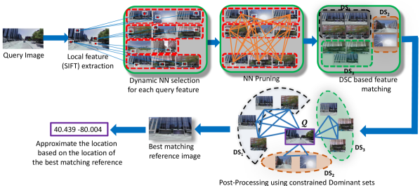
Fig. 1 depicts the overview of the proposed approach. Given a set of reference images, e.g., taken from Google Street View, we extract local features (hereinafter referred as reference features) using SIFT from each reference image. We then organize them in a k-means tree [40].
First, for each local feature extracted from the query image (hereinafter referred as query feature), we dynamically collect nearest neighbors based on how distinctive the two nearest neighbors are relative to their corresponding query feature. Then, we remove query features, along with their corresponding reference features, if the ratio of the distance between the first and the last nearest neighbor is too large (Sec. 3.1). If so, it means that the query feature is not very informative for geo-localization, and is not worth keeping for further processing. In the next step, we formalize the problem of finding matching reference features to query features as a DSC (Dominant Set Clustering) problem, that is, selecting reference features which form a coherent and most compact set (Sec. 3.2). Finally, we employ constrained dominant-set-based post-processing step to choose the best matching reference image and use the location of the strongest match as an estimation of the location of the query image (Sec. 4).
3.1 Dynamic Nearest Neighbor Selection and Query Feature Pruning
For each of query features detected in the query image, we collect their corresponding nearest neighbors (NN). Let be the nearest neighbor of query feature , and and , where represents the set cardinality and is the set of NNs of the query feature. In this work, we propose a dynamic NNs selection technique based on how distinctive two consecutive elements are in a ranked list of neighbors for a given query feature, and employ different number of nearest neighbors for each query feature.
Input: the query feature () and all its nearest neighbors extracted from K-means tree
Output: Selected Nearest Neighbors for the query feature
As shown in Algorithm (1), we add the NN of the query feature, , if the ratio of the two consecutive NN is greater than , otherwise we stop. In other words, in the case of a query feature which is not very discriminative, i.e., most of its NNs are very similar to each other, the algorithm continues adding NNs until a distinctive one is found. In this way, less discriminative query features will use more NNs to account for their ambiguity, whereas more discriminative query features will be compared with fewer NNs.
Query Feature Pruning. For the geo-localization task, most of the query features that are detected from moving objects (such as cars) or the ground plane, do not convey any useful information. If such features are coarsely identified and removed prior to performing the feature matching, that will reduce the clutter and computation cost for the remaining features. Towards this end, we use the following pruning constraint which takes into consideration distinctiveness of the first and the last NN. In particular, if , where represents an operator which returns the local descriptor of the argument node, then is removed, otherwise it is retained. That is, if the first NN is similar to the last NN (less than ), then the corresponding query feature along with its NNs are pruned since it is expected to be uninformative.
We empirically set both thresholds, and , in Algorithm (1) and pruning step, respectively, to 0.7 and keep them fixed for all tests.
3.2 Multiple Feature Matching Using Dominant Sets
3.2.1 The Dominant Set Framework
The dominant set framework is a pairwise clustering approach [41], based on the notion of a dominant set, which can be seen as an edge-weighted generalization of a clique. The approach is a fast and efficient framework for pairwise clustering and has been used to solve multiple problems, such as data association in tracking [42] as well as group detection [43].
In an attempt to formally capture this notion, we present some notations and definitions. The data to be clustered is defined as a graph , where and denote the set of nodes (of cardinality ), edges, node weights and edge weights, respectively. For a non-empty subset , , and , where and represent nodes in a graph , we define , where is the corresponding affinity matrix of graph . This quantity measures the relative similarity between nodes and , with respect to the average similarity between node and its neighbors in . Note that can be either positive or negative. Next, to each vertex we assign a weight defined recursively as follows:
| (1) |
where means set without the element . Intuitively, gives us a measure of the overall similarity between vertex and the vertices of , with respect to the overall similarity among the vertices in . Therefore, a positive indicates that adding into its neighbors in will increase the internal coherence of the set, whereas in the presence of a negative value we expect the overall coherence to be decreased. The total weight of is computed as .
A non-empty subset of vertices such that for any non-empty , is said to be a dominant set if:
| (2) |
These conditions correspond to the two main properties of a cluster: the first regards internal homogeneity, whereas the second regards external inhomogeneity.
Example: Let us consider a graph with nodes , which forms a coherent group (dominant set) with edge weights 20, 21 and 22 as shown in Fig. 2(a). Now, let us try to add a node to the graph which is highly similar to the set {1,2,3} with edge weights of 30, 35 and 41 (see Fig. 2(b)). Here, we can see that adding node {4} to the set increases the overall similarity of the new set {1,2,3,4}, that can be seen from the fact that the weight associated to the node {4} with respect to the set {1,2,3,4} is positive, . On the contrary, when adding node {5} which is less similar to the set {1,2,3,4} (edge weight of 1 - Fig. 2(c)) the overall similarity of the new set {1,2,3,4,5} decreases, since we are adding to the set something less similar with respect to the internal similarity. This is reflected by the fact that the weight associated to node {5} with respect to the set {1,2,3,4,5} is less than zero .
From the definition of a dominant set in (2) the set {1,2,3,4} (Fig. 2 (b)) forms a dominant set, as it satisfies both criteria (internal coherence and external incoherence). While the weight associated to the node out side of the set (dominant set) is less than zero, .

The main result presented in [41] provides a one-to-one relation between dominant sets and strict local maximizers of the following standard quadratic optimization problem:
| (3) |
where
which is called standard simplex of . Specifically, in [41] it is shown that if is a dominant subset of vertices, then its weighted characteristic vector, which lies in ,
is a strict local solution of (3). Conversely, under mild conditions, if is a strict local solution of (3), then its support is a dominant set. Here, the support of a vector is the set of indices corresponding to its positive components, that is . By virtue of this result, a dominant set can be found by localizing a local solution of (3) and then picking up its support.
3.2.2 Similarity Function and Dynamics for Multiple Feature Matching
In our framework, the set of nodes, , represents all NNs for each query feature which survives the pruning step. The edge set is defined as , which signifies that all the nodes in are connected as long as their corresponding query features are not the same. The edge weight, is defined as , where represents an operator which returns the global descriptor of the parent image of the argument node and is empirically set to . The edge weight, , represents a similarity between nodes and in terms of the global features of their parent images. The node score, , is defined as . The node score shows how similar the node is with its corresponding query feature in terms of its local features.
Matching the query features to the reference features requires identifying the correct NNs from the graph which maximize the weight, that is, selecting a node (NN) which forms a coherent (highly compact) set in terms of both global and local feature similarities.
Affinity matrix represents the global similarity among reference images, which is built using GPS locations as a global feature and a node score which shows how similar the reference image is with its corresponding query feature in terms of their local features. We formulate the following optimization problem, a more general form of the dominant set formulation:
| (4) |
The affinity and the score are computed as follows:
| (5) | ||||
| (6) |
General quadratic optimization problems, like (4), are known to be NP-hard [44]. However, in relaxed form, standard quadratic optimization problems can be solved using many algorithms which make full systematic use of data constellations. Off-the-shelf procedures find a local solution of (4), by following the paths of feasible points provided by game dynamics based on evolutionary game theory.
Interestingly, the general quadratic optimization problem can be rewritten in the form of standard quadratic problem. A principled way to do that is to follow the result presented in [45], which shows that maximizing the general quadratic problem over the simplex can be homogenized as follows. Maximizing is equivalent to maximizing , where and = , where denotes the standard basis vector in . This can be easily proved by noting that the problem is solved in the simplex.
-
,
-
,
-
,
-
.
As can be inferred from the formulation of our multiple NN feature matching problem, DSC can be essentially used for solving the optimization problem. Therefore, by solving DSC for the graph , the optimal solution that has the most agreement in terms of local and global features will be found. Next, we introduce some useful dynamics from evolutionary game theory which allow us to efficiently and effectively match reference features to the query features.
The standard approach for finding the local maxima of problem (3), as used in [41], is to use replicator dynamics - a well-known family of algorithms from evolutionary game theory inspired by Darwinian selection processes. Variety of StQP applications [46, 47, 41, 48, 49] have proven the effectiveness of replicator dynamics. However, its computational complexity, which is for problems involving variables, prevents it from being used in large-scale applications. Its exponential variant, though it reduces the number of iterations needed for the algorithm to find a solution, suffers from a per-step quadratic complexity.
In this work, we adopt a new class of evolutionary game dynamics called infection-immunization dynamics (InImDyn), which have been shown to have a linear time/space complexity for solving standard quadratic programs. In [4], it has been shown that InImDyn is orders of magnitude faster but as accurate as the replicator dynamics.
The dynamics, inspired by infection and immunization processes summarized in Algorithm (2), finds the optimal solution by iteratively refining an initial distribution . The process allows for invasion of an infective distribution that satisfies the inequality , and combines linearly and (line 7 of Algorithm (2)), thereby engendering a new population which is immune to and guarantees a maximum increase in the expected payoff. A selective function, , returns an infective strategy for distribution if it exists, or otherwise (line 2 of Algorithm (2)). Selecting a strategy which is infective for the current population , the extent of the infection, , is then computed in lines 3 to 6 of Algorithm (2).
By reiterating this process of infection and immunization the dynamics drives the population to a state that cannot be infected by any other strategy. If this is the case then is an equilibrium or fixed point under the dynamics. The refinement loop of Algorithm (2) controls the number of iterations allowing them to continue until is with in the range of the tolerance and we emperically set to . The range is computed as = .
Input: payoff matrix , initial distribution and tolerance .
Output: Fixed point
As it can be inferred from the above formulation of dominant sets, finding the strict local solution of (3) coincides with finding the best matching reference features to the query features. It is important to note that, since our solution is a local solution and we do not know which local solution includes the best matching reference image, we determine several (typically three) locally optimal solutions. Unlike most of the previous approaches, which perform a simple voting scheme to select the best matching reference image, we introduce a post processing step utilizing a variant of dominant set called constrained dominant set, which is discussed briefly in the next section.
4 Post processing using constrained dominant sets
Up to now, we devised a method to collect matching reference features corresponding to our query features. The next task is to select one reference image, based on feature matching between query and reference features, which best matches the query image. To do so, most of the previous methods follow a simple voting scheme, that is, the matched reference image with the highest vote is considered as the best match.
This approach has two important shortcomings. First, if there are equal votes for two or more reference images (which happens quite often), it will randomly select one, which makes it prone to outliers. Second, a simple voting scheme does not consider the similarity between the query image and the candidate reference images at the global level, but simply accounts for local matching of features. Therefore, we deal with this issue by proposing a post processing step, which considers the comparison of the global features of the images and employs constrained dominant set, a framework that generalizes the dominant sets formulation and its variant [41, 50].
4.1 Constrained Dominant Sets Framework
In our post processing step, the user-selected query and the matched reference images are related using their global features and a unique local solution is then searched which contains the union of all the dominant sets containing the query. As customary, the resulting solution will be globally consistent both with the reference images and the query image and due to the notion of centrality, each element in the resulting solution will have a membership score, which depicts how similar a given reference image is with the rest of the images in the cluster. So, by virtue of this property of constrained dominant sets, we will select the image with the highest membership score as the final best matching reference image and approximate the location of the query with the GPS location of the best matched reference image.
In this section, we review the basic definitions and properties of constrained dominant sets, as introduced in [51]. Given a user specified query, , we define the graph , where the edges are defined as , i.e., all the nodes are connected as long as they do not belong to different local maximizers, , which represents the extracted dominant set. The set of nodes represents all matched reference images (local maximizers) and query image, . The edge weight is defined as:
where is an operator which returns the global similarity of two given images and , that is, , represents a sub-matrix of , which contains only members of , normalized by its maximum value and finally returns the normalized affinity between the and members of . The graph can be represented by an affinity matrix , where is the number of nodes in the graph.
Given a parameter , let us define the following parameterized variant of program (3):
| (7) |
where is the diagonal matrix whose diagonal elements are set to 1 in correspondence to the vertices contained in (a set without the element ) and to zero otherwise.
Let , with and let , where is the largest eigenvalue of the principal submatrix of indexed by the elements of . If is a local maximizer of in , then . A complete proof can be found in [51].
The above result provides us with a simple technique to determine dominant-set clusters containing user-specified query vertices. Indeed, if is a vertex selected by the user, by setting
| (8) |
we are guaranteed that all local solutions of (7) will have a support that necessarily contains elements of .
The performance of our post processing may vary dramatically among queries and we do not know in advance which global feature plays a major role. Figs. 3 and 4 show illustrative cases of different global features. In the case of Fig. 3, HSV color histograms and GIST provide a wrong match (dark red node for HSV and dark green node for GIST), while both CNN-based global features (CNN6 and CNN7) matched it to the right reference image (yellow node). The second example, Fig. 4, shows us that only CNN6 feature localized it to the right location while the others fail. Recently, fusing different retrieval methods has been shown to enhance the overall retrieval performance [52, 53].
Motivated by [52] we dynamically assign a weight, based on the effectiveness of a feature, to all global features based on the area under normalized score between the query and the matched reference images. The area under the curve is inversely proportional to the effectiveness of a feature. More specifically, let us suppose to have global features and the distance between the query and the matched reference image ( ), based on the global feature (), is computed as: , where represents an operator which returns the global descriptor of the argument node. Let the area under the normalized score of be . The weight assigned for feature is then computed as .
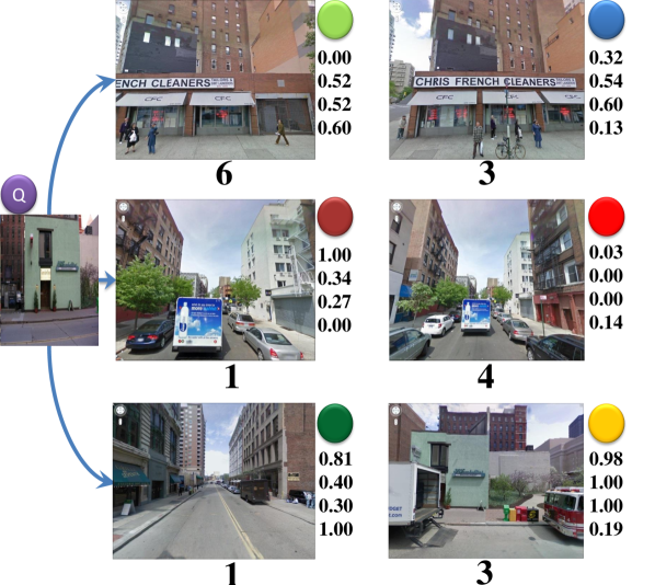
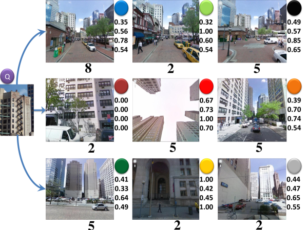
Figs. 3 and 4 show illustrative cases of some of the advantages of having the post processing step. Both cases show the disadvantage of localization following heuristic approaches, as in [1, 2], to voting and selecting the reference image that matches to the query. In each case, the matched reference image with the highest number of votes (shown under each image) is the first node of the first extracted dominant set, but represents a wrong match. Both cases (Figs. 3 and 4) also demonstrate that the KNN-based matching may lead to a wrong localization. For example, by choosing HSV histogram as a global feature, the KNN approach chooses as best match the dark red node in Fig. 3 and the yellow node in Fig. 4 (both with min-max value to 1.00). Moreover, it is also evident that choosing the best match using the first extracted local solution (i.e., the light green node in Fig. 3 and blue node in Fig. 4), as done in [2], may lead to a wrong localization, since one cannot know in advance which local solution plays a major role. In fact, in the case of Fig. 3, the third extracted dominant set contains the right matched reference image (yellow node), whereas in the case of Fig. 4 the best match is contained in the first local solution (the light green node).
The similarity between query and the corresponding matched reference images is computed using their global features such as HSV histogram, GIST [54] and CNN (CNN6 and CNN7 are Convolutional Neural Network features extracted from ReLU6 and FC7 layers of pre-trained network, respectively [55]). For the different advantages and disadvantages of the global features, we refer interested readers to [2].
Fig. 3 shows the top three extracted dominant sets with their corresponding frequency of the matched reference images (at the bottom of each image). Let be the number (cardinality) of local features, which belongs to reference image from the extracted sets and the total number of matched reference images be . We build an affinity matrix of size (e.g., for the example in Fig. 3, the size is 19 ). Fig. 5 shows the reduced graph for the matched reference images shown in Fig. 3. Fig. 5 upper left, shows the part of the graph for the post processing. It shows the relation that the query has with matched reference images. The bottom left part of the figure shows how one can get the full graph from the reduced graph. For the example in Fig. 5, .
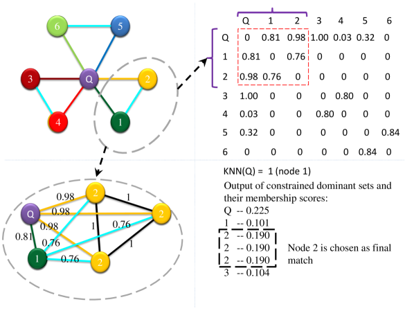
The advantages of using constrained dominant sets are numerous. First, it provides a unique local (and hence global) solution whose support coincides with the union of all dominant sets of , which contains the query. Such solution contains all the local solutions which have strong relation with the user-selected query. As it can be observed in Fig. 5 (bottom right), the Constrained Dominant Set which contains the query , , is the union of all overlapping dominant sets (the query, one green, one dark red and three yellow nodes) containing the query as one of the members. If we assume to have no cyan link between the green and yellow nodes, as long as there is a strong relation between the green node and the query, will not be affected. In addition, due to the noise, the strong affinity between the query and the green node may be reduced, while still keeping the strong relation with the cyan link which, as a result, will preserve the final result. Second, in addition to fusing all the local solutions leveraging the notion of centrality, one of the interesting properties of dominant set framework is that it assigns to each image a score corresponding to how similar it is to the rest of the images in the solution. Therefore, not only it helps selecting the best local solution, but also choosing the best final match from the chosen local solution. Third, an interesting property of constrained dominant sets approach is that it not only considers the pairwise similarity of the query and the reference images, but also the similarity among the reference images. This property helps the algorithm avoid assignment of wrong high pairwise affinities. As an example, with reference to Fig. 5, if we consider the nodes pairwise affinities, the best solution will be the dark red node (score 1.00). However, using constrained dominant sets and considering the relation among the neighbors, the solution bounded by the red dotted rectangle can be found, and by choosing the node with the highest membership score, the final best match is the yellow node which is more similar to the query image than the reference image depicted by the dark red node (see Fig. 3).
5 Experimental Results
5.1 Dataset Description
We evaluate the proposed algorithm using publicly available reference data sets of over 102k Google street view images [2] and a new dataset, WorldCities, of high resolution 300k Google street view images collected for this work. The 360 degrees view of each place mark is broken down into one top and four side view images. The WorldCities dataset is publicly available. 111http://www.cs.ucf.edu/~haroon/UCF-Google-Streetview-II-Data/UCF-Google-Streetview-II-Data.zip
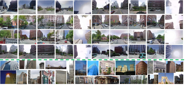
The 102k Google street view images dataset covers 204 Km of urban streets and the place marks are approximately 12 m apart. It covers downtown and the neighboring areas of Orlando, FL; Pittsburgh, PA and partially Manhattan, NY. The WorldCities dataset is a new high resolution reference dataset of 300k street view images that covers 14 different cities from different parts of the world: Europe (Amsterdam, Frankfurt, Rome, Milan and Paris), Australia (Sydney and Melbourne), USA (Vegas, Los Angeles, Phoenix, Houston, San Diego, Dallas, Chicago). Existence of similarity in buildings around the world, which can be in terms of their wall designs, edges, shapes, color etc, makes the dataset more challenging than the other. Fig. 6 (top four rows) shows sample reference images taken from different place marks.
For the test set, we use 644 and 500 GPS-tagged user uploaded images downloaded from Picasa, Flickr and Panoramio for the 102k Google street view images and WorldCities datasets, respectively. Fig. 6 (last two rows) shows sample test images. Throughout our experiment, we use the all the reference images from around the world to find the best match with the query image, not just with the ground truth city only.
5.2 Quantitative Comparison With Other Methods
5.2.1 Performance on the 102k Google street view images Dataset
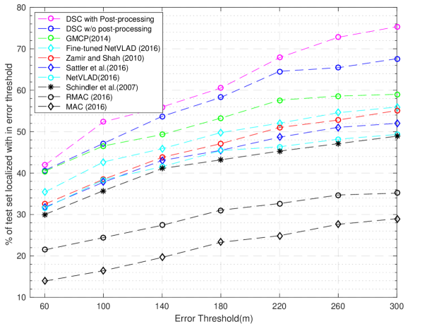
The proposed approach has been then compared with the results obtained by state-of-the-art methods. In Fig. 7, the horizontal axes shows the error threshold in meters and the vertical axes shows the percentage of the test set localized within a particular error threshold. Since the scope of this work is an accurate image localization at a city-scale level, test set images localized above 300 meter are considered a failure.
The black (-*-) curve shows localization result of the approach proposed in [16] which uses vocabulary tree to localize images. The red (-o-) curve depicts the results of [1] where they only consider the first NN for each query feature as best matches which makes the approach very sensitive to the query features they select. Moreover, their approach suffers from lacking global feature information. The green (-o-) curve illustrates the localization results of [2] which uses generalized maximum clique problem (GMCP) to solve feature matching problem and follows voting scheme to select the best matching reference image. The black (-o- and ) curves show localization results of MAC and RMAC, (regional) maximum activation of convolutions ([56, 57]). These approaches build compact feature vectors that encode several image regions without the need to feed multiple inputs to the network. The cyan (-o-) curve represents localization result of NetVLAD [18] which aggregates mid-level (conv5) convolutional features extracted from the entire image into a compact single vector representation amenable to effici,ent indexing. The cyan () curve depicts localization result of NetVLAD but finetuned on our dataset. The blue () curve show localizaton result of approach proposed in [17] which exploits geometric relations between different database images retrieved by a query to handle geometric burstness. The blue (-o-) curve shows results from our baseline approach, that is, we use voting scheme to select best match reference image and estimate the location of the query image. We are able to make a 10% improvement w.r.t the other methods with only our baseline approach (without post processing). The magenta (-o-) curve illustrates geo-localization results of our proposed approach using dominant set clustering based feature matching and constrained dominant set clustering based post processing. As it can be seen, our approach shows about 20% improvement over the state-of-the-art techniques.
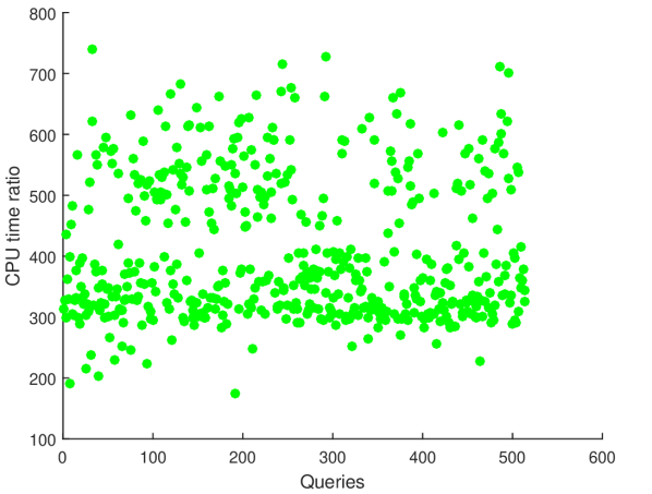
Computational Time. Fig. 8, on the vertical axis, shows the ratio between GMCP (numerator) and our approach (denominator) in terms of CPU time taken for each query images to be localized. As it is evident from the plot, this ratio can range from 200 (our approach 200x faster than GMCP) to a maximum of even 750x faster.
5.2.2 Performance on the WorldCities Dataset
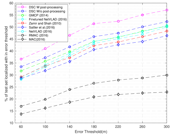
We have also compared the performance of different algorithms on the new dataset of 300k Google street view images created by us. Similarly to the previous tests, Fig. 9 reports the percentage of the test set localized within a particular error threshold. Since the new dataset is relatively more challenging, the overall performance achieved by all the methods is lower compared to 102k image dataset.
From bottom to top of the graph in Fig. 9 we present the results of [56, 57] black ( and -o-), [17] blue (), [1] red (-o-), [18] cyan (-o-), fine tuned [18] cyan (), [2] green (-o-), our baseline approach without post processing blue (-o-) and our final approach with post processing magenta (-o-) . The improvements obtained with our method are lower than in the other dataset, but still noticeable (around 2% for the baseline and 7% for the final approach).
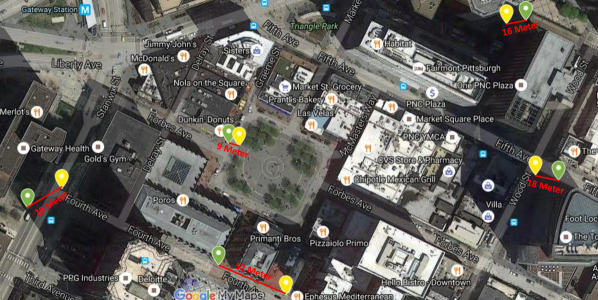
Some qualitative results for Pittsburgh, PA are presented in Fig. 10.
5.3 Analysis
5.3.1 Outlier Handling
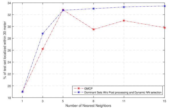
In order to show that our dominant set-based feature matching technique is robust in handling outliers, we conduct an experiment by fixing the number of NNs (disabling the dynamic selection of NNs) to different numbers. It is obvious that the higher the number of NNs are considered for each query feature, the higher will be the number of outlier NNs in the input graph, besides the increased computational cost and an elevated chance of query features whose NNs do not contain any inliers surviving the pruning stage.
Fig. 11 shows the results of geo-localization obtained by using GMCP and dominant set based feature matching on 102K Google street view images [2]. The graph shows the percentage of the test set localized within the distance of 30 meters as a function of number of NNs. The blue curve shows the results using dominant sets: it is evident that when the number of NNs increases, the performance improves despite the fact that more outliers are introduced in the input graph. This is mainly because our framework takes advantage of the few inliers that are added along with many outliers. The red curve shows the results of GMCP based localization and as the number of NNs increase the results begin to drop. This is mainly due to the fact that their approach imposes hard constraint that at least one matching reference feature should be selected for each query feature whether or not the matching feature is correct.
5.3.2 Effectiveness of the Proposed Post Processing
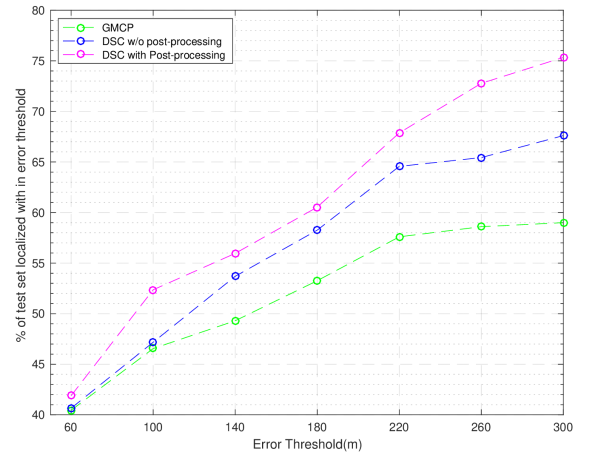
In order to show the effectiveness of the post processing step, we perform an experiment comparing our constrained dominant set based post processing with a simple voting scheme to select the best matching reference image. The GPS information of the best matching reference image is used to estimate the location of the query image. In Fig. 13, the vertical axis shows the percentage of the test set localized within a particular error threshold shown in the horizontal axis (in meters). The blue and magenta curves depict geo-localization results of our approach using a simple voting scheme and constrained dominant sets, respectively. The green curve shows the results from GMCP based geo-localization. As it is clear from the results, our approach with post processing exhibits superior performance compared to both GMCP and our baseline approach.
Since our post-processing algorithm can be easily plugged in to an existing retrieval methods, we perform another experiment to determine how much improvement we can achieve by our post processing. We use [19, 56, 57] methods to obtain candidate reference images and employ as an edge weight the similarity score generated by the corresponding approaches. Table I reports, for each dataset, the first row shows rank-1 result obtained from the existing algorithms while the second row (w_post) shows rank-1 result obtained after adding the proposed post-processing step on top of the retrieved images. For each query, we use the first 20 retrieved reference images. As the results demonstrate, Table I, we are able to make up to 7% and 4% improvement on 102k Google street view images and WorldCities datasets, respectively. We ought to note that, the total additional time required to perform the above post processing, for each approach, is less than 0.003 seconds on average.
| NetVLAD | NetVLAD* | RMAC | MAC | ||
| Dts 1 | Rank1 | 49.2 | 56.00 | 35.16 | 29.00 |
| w_post | 51.60 | 58.05 | 40.18 | 36.30 | |
| Dts 2 | Rank1 | 50.00 | 50.61 | 29.96 | 22.87 |
| w_post | 53.04 | 52.23 | 33.16 | 26.31 |
The NetVLAD results are obtained from the features generated using the best trained model downloaded from the author’s project page [19]. It’s fine-tuned version (NetVLAD*) is obtained from the model we fine-tuned using images within 24m range as a positive set and images with GPS locations greater than 300m as a negative set.
The MAC and RMAC results are obtained using MAC and RMAC representations extracted from fine-tuned VGG networks downloaded from the authors webpage [56, 57].
5.3.3 Assessment of Global Features Used in Post Processing Step
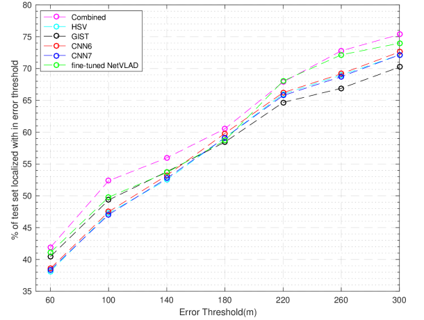
The input graph for our post processing step utilizes the global similarity between the query and the matched reference images. Wide variety of global features can be used for the proposed technique. In our experiments, the similarity between query and the corresponding matched reference images is computed between their global features, using HSV, GIST, CNN6, CNN7 and fine-tuned NetVLAD. The performance of the proposed post processing technique highly depends on the discriminative ability of the global features used to built the input graph.
Depending on how informative the feature is, we dynamically assign a weight for each global feature based on the area under the normalized score between the query and the matched reference images. To show the effectiveness of this approach, we perform an experiment to find the location of our test set images using both individual and combined global features. Fig. 12 shows the results attained by using fine-tuned NetVLAD, CNN7, CNN6, GIST, HSV and by combining them together. The combination of all the global features outperforms the individual feature performance, demonstrating the benefits of fusing the global features based on their discriminative abilities for each query.
6 Conclusion and Future Work
In this paper, we proposed a novel framework for city-scale image geo-localization. Specifically, we introduced dominant set clustering-based multiple NN feature matching approach. Both global and local features are used in our matching step in order to improve the matching accuracy. In the experiments, carried out on two large city-scale datasets, we demonstrated the effectiveness of post processing employing the novel constrained dominant set over a simple voting scheme. Furthermore, we showed that our proposed approach is 200 times, on average, faster than GMCP-based approach [2]. Finally, the newly-created dataset (WorldCities) containing more than 300k Google Street View images used in our experiments will be made available to the public for research purposes.
As a natural future direction of research, we can extend the results of this work for estimating the geo-spatial trajectory of a video in a city-scale urban environment from a moving camera with unknown intrinsic camera parameters.
References
- [1] A. R. Zamir and M. Shah, “Accurate image localization based on google maps street view,” in European Conference on Computer Vision. Springer, 2010, pp. 255–268.
- [2] ——, “Image geo-localization based on multiple nearest neighbor feature matching using generalized graphs,” IEEE Trans. Pattern Anal. Mach. Intell., vol. 36, no. 8, pp. 1546–1558, 2014.
- [3] S. Rota Bulò and I. M. Bomze, “Infection and immunization: A new class of evolutionary game dynamics,” Games and Economic Behavior, vol. 71, no. 1, pp. 193–211, 2011.
- [4] S. R. Bulò, M. Pelillo, and I. M. Bomze, “Graph-based quadratic optimization: A fast evolutionary approach,” Computer Vision and Image Understanding, vol. 115, no. 7, pp. 984–995, 2011.
- [5] Y. Avrithis, Y. Kalantidis, G. Tolias, and E. Spyrou, “Retrieving landmark and non-landmark images from community photo collections,” in Proceedings of the 18th ACM international conference on Multimedia. ACM, 2010, pp. 153–162.
- [6] D. M. Chen, G. Baatz, K. Köser, S. S. Tsai, R. Vedantham, T. Pylvänäinen, K. Roimela, X. Chen, J. Bach, M. Pollefeys et al., “City-scale landmark identification on mobile devices,” in Computer Vision and Pattern Recognition (CVPR), 2011 IEEE Conference on. IEEE, 2011, pp. 737–744.
- [7] T. Quack, B. Leibe, and L. Van Gool, “World-scale mining of objects and events from community photo collections,” in Proceedings of the 2008 international conference on Content-based image and video retrieval. ACM, 2008, pp. 47–56.
- [8] Y.-T. Zheng, M. Zhao, Y. Song, H. Adam, U. Buddemeier, A. Bissacco, F. Brucher, T.-S. Chua, and H. Neven, “Tour the world: building a web-scale landmark recognition engine,” in Computer vision and pattern recognition, 2009. CVPR 2009. IEEE conference on. IEEE, 2009, pp. 1085–1092.
- [9] H. Jin Kim, E. Dunn, and J.-M. Frahm, “Predicting good features for image geo-localization using per-bundle vlad,” in Proceedings of the IEEE International Conference on Computer Vision, 2015, pp. 1170–1178.
- [10] J. Hays and A. A. Efros, “Im2gps: estimating geographic information from a single image,” in Computer Vision and Pattern Recognition, 2008. CVPR 2008. IEEE Conference on. IEEE, 2008, pp. 1–8.
- [11] ——, “Large-scale image geolocalization,” in Multimodal Location Estimation of Videos and Images. Springer, 2015, pp. 41–62.
- [12] T. Weyand, I. Kostrikov, and J. Philbin, “Planet-photo geolocation with convolutional neural networks,” arXiv preprint arXiv:1602.05314, 2016.
- [13] S. Gammeter, L. Bossard, T. Quack, and L. Van Gool, “I know what you did last summer: object-level auto-annotation of holiday snaps,” in 2009 IEEE 12th International Conference on Computer Vision. IEEE, 2009, pp. 614–621.
- [14] E. Johns and G.-Z. Yang, “From images to scenes: Compressing an image cluster into a single scene model for place recognition,” in 2011 International Conference on Computer Vision. IEEE, 2011, pp. 874–881.
- [15] D. J. Crandall, L. Backstrom, D. Huttenlocher, and J. Kleinberg, “Mapping the world’s photos,” in Proceedings of the 18th international conference on World wide web. ACM, 2009, pp. 761–770.
- [16] G. Schindler, M. A. Brown, and R. Szeliski, “City-scale location recognition,” in IEEE Computer Society Conference on Computer Vision and Pattern Recognition (CVPR), Minneapolis, Minnesota, 2007.
- [17] T. Sattler, M. Havlena, K. Schindler, and M. Pollefeys, “Large-scale location recognition and the geometric burstiness problem,” in 2016 IEEE Conference on Computer Vision and Pattern Recognition, CVPR 2016, Las Vegas, NV, USA, June 27-30, 2016, 2016, pp. 1582–1590.
- [18] R. Arandjelovic, P. Gronát, A. Torii, T. Pajdla, and J. Sivic, “Netvlad: CNN architecture for weakly supervised place recognition,” in 2016 IEEE Conference on Computer Vision and Pattern Recognition, CVPR 2016, Las Vegas, NV, USA, June 27-30, 2016, 2016, pp. 5297–5307.
- [19] A. Torii, J. Sivic, M. Okutomi, and T. Pajdla, “Visual place recognition with repetitive structures,” IEEE Trans. Pattern Anal. Mach. Intell., vol. 37, no. 11, pp. 2346–2359, 2015.
- [20] B. Zeisl, T. Sattler, and M. Pollefeys, “Camera pose voting for large-scale image-based localization,” in 2015 IEEE International Conference on Computer Vision, ICCV 2015, Santiago, Chile, December 7-13, 2015, 2015, pp. 2704–2712.
- [21] S. Agarwal, N. Snavely, I. Simon, S. M. Seitz, and R. Szeliski, “Building rome in a day,” in 2009 IEEE 12th international conference on computer vision. IEEE, 2009, pp. 72–79.
- [22] Y. Li, N. Snavely, D. Huttenlocher, and P. Fua, “Worldwide pose estimation using 3d point clouds,” in European Conference on Computer Vision. Springer, 2012, pp. 15–29.
- [23] T. Sattler, B. Leibe, and L. Kobbelt, “Fast image-based localization using direct 2d-to-3d matching,” in 2011 International Conference on Computer Vision. IEEE, 2011, pp. 667–674.
- [24] ——, “Improving image-based localization by active correspondence search,” in European Conference on Computer Vision. Springer, 2012, pp. 752–765.
- [25] E. Kalogerakis, O. Vesselova, J. Hays, A. A. Efros, and A. Hertzmann, “Image sequence geolocation with human travel priors,” in 2009 IEEE 12th International Conference on Computer Vision. IEEE, 2009, pp. 253–260.
- [26] G. Vaca-Castano, A. R. Zamir, and M. Shah, “City scale geo-spatial trajectory estimation of a moving camera,” in Computer Vision and Pattern Recognition (CVPR), 2012 IEEE Conference on. IEEE, 2012, pp. 1186–1193.
- [27] A. Hakeem, R. Vezzani, M. Shah, and R. Cucchiara, “Estimating geospatial trajectory of a moving camera,” in 18th International Conference on Pattern Recognition (ICPR’06), vol. 2. IEEE, 2006, pp. 82–87.
- [28] C.-Y. Chen and K. Grauman, “Clues from the beaten path: Location estimation with bursty sequences of tourist photos,” in Computer Vision and Pattern Recognition (CVPR), 2011 IEEE Conference on. IEEE, 2011, pp. 1569–1576.
- [29] T.-Y. Lin, S. Belongie, and J. Hays, “Cross-view image geolocalization,” in Proceedings of the IEEE Conference on Computer Vision and Pattern Recognition, 2013, pp. 891–898.
- [30] T.-Y. Lin, Y. Cui, S. Belongie, and J. Hays, “Learning deep representations for ground-to-aerial geolocalization,” in 2015 IEEE Conference on Computer Vision and Pattern Recognition (CVPR). IEEE, 2015, pp. 5007–5015.
- [31] S. Workman, R. Souvenir, and N. Jacobs, “Wide-area image geolocalization with aerial reference imagery,” in Proceedings of the IEEE International Conference on Computer Vision, 2015, pp. 3961–3969.
- [32] N. Jacobs, S. Satkin, N. Roman, R. Speyer, and R. Pless, “Geolocating static cameras,” in 2007 IEEE 11th International Conference on Computer Vision. IEEE, 2007, pp. 1–6.
- [33] S. Ramalingam, S. Bouaziz, P. Sturm, and M. Brand, “Skyline2gps: Localization in urban canyons using omni-skylines,” in Intelligent Robots and Systems (IROS), 2010 IEEE/RSJ International Conference on. IEEE, 2010, pp. 3816–3823.
- [34] R. Arandjelović and A. Zisserman, “Dislocation: Scalable descriptor distinctiveness for location recognition,” in Asian Conference on Computer Vision. Springer, 2014, pp. 188–204.
- [35] A. Bergamo, S. N. Sinha, and L. Torresani, “Leveraging structure from motion to learn discriminative codebooks for scalable landmark classification,” in Proceedings of the IEEE Conference on Computer Vision and Pattern Recognition, 2013, pp. 763–770.
- [36] S. Cao and N. Snavely, “Graph-based discriminative learning for location recognition,” in Proceedings of the IEEE Conference on Computer Vision and Pattern Recognition, 2013, pp. 700–707.
- [37] P. Gronat, G. Obozinski, J. Sivic, and T. Pajdla, “Learning and calibrating per-location classifiers for visual place recognition,” in Proceedings of the IEEE Conference on Computer Vision and Pattern Recognition, 2013, pp. 907–914.
- [38] A. Torii, J. Sivic, T. Pajdla, and M. Okutomi, “Visual place recognition with repetitive structures,” in Proceedings of the IEEE Conference on Computer Vision and Pattern Recognition, 2013, pp. 883–890.
- [39] Q. Hao, R. Cai, Z. Li, L. Zhang, Y. Pang, and F. Wu, “3d visual phrases for landmark recognition,” in Computer Vision and Pattern Recognition (CVPR), 2012 IEEE Conference on. IEEE, 2012, pp. 3594–3601.
- [40] M. Muja and D. G. Lowe, “Fast approximate nearest neighbors with automatic algorithm configuration,” in VISAPP 2009 - Proceedings of the Fourth International Conference on Computer Vision Theory and Applications, Lisboa, Portugal, February 5-8, 2009 - Volume 1, 2009, pp. 331–340.
- [41] M. Pavan and M. Pelillo, “Dominant sets and pairwise clustering,” IEEE Trans. Pattern Anal. Mach. Intell., vol. 29, no. 1, pp. 167–172, 2007.
- [42] Y. T. Tesfaye, E. Zemene, M. Pelillo, and A. Prati, “Multi-object tracking using dominant sets,” IET computer vision, vol. 10, pp. 289–298, 2016.
- [43] S. Vascon, E. Z. Mequanint, M. Cristani, H. Hung, M. Pelillo, and V. Murino, “Detecting conversational groups in images and sequences: A robust game-theoretic approach,” Computer Vision and Image Understanding, vol. 143, pp. 11–24, 2016.
- [44] R. Horst, P. Pardalos, and N. Van Thoai, Introduction to Global Optimization, ser. Nonconvex Optimization and Its Applications. Kluwer Academic Publishers, Dordrecht/Boston/London, 2000.
- [45] I. M. Bomze, “On standard quadratic optimization problems,” J. Global Optimization, vol. 13, no. 4, pp. 369–387, 1998.
- [46] ——, “Evolution towards the maximum clique,” J. Global Optimization, vol. 10, no. 2, pp. 143–164, 1997.
- [47] K. Müller, J. Neumann, M. Grigutsch, D. Y. von Cramon, and G. Lohmann, “Detecting groups of coherent voxels in functional mri data using spectral analysis and replicator dynamics,” Journal of Magnetic Resonance Imaging, vol. 26, no. 6, pp. 1642–1650, 2007.
- [48] M. Pelillo, “Replicator dynamics in combinatorial optimization,” in Encyclopedia of Optimization, Second Edition, 2009, pp. 3279–3291.
- [49] S. Todorovic and N. Ahuja, “Region-based hierarchical image matching,” International Journal of Computer Vision, vol. 78, no. 1, pp. 47–66, 2008.
- [50] M. Pavan and M. Pelillo, “Dominant sets and hierarchical clustering,” in ICCV, 2003, pp. 362–369.
- [51] E. Zemene and M. Pelillo, “Interactive image segmentation using constrained dominant sets,” in ECCV, 2016, pp. 278–294.
- [52] L. Zheng, S. Wang, L. Tian, F. He, Z. Liu, and Q. Tian, “Query-adaptive late fusion for image search and person re-identification,” in CVPR, 2015, pp. 1741–1750.
- [53] S. Zhang, M. Yang, T. Cour, K. Yu, and D. N. Metaxas, “Query specific rank fusion for image retrieval,” IEEE Trans. Pattern Anal. Mach. Intell., vol. 37, no. 4, pp. 803–815, 2015.
- [54] A. Oliva and A. Torralba, “Modeling the shape of the scene: A holistic representation of the spatial envelope,” International Journal of Computer Vision, vol. 42, no. 3, pp. 145–175, 2001.
- [55] K. Simonyan and A. Zisserman, “Very deep convolutional networks for large-scale image recognition,” arXiv preprint arXiv:1409.1556, 2014.
- [56] G. Tolias, R. Sicre, and H. Jégou, “Particular object retrieval with integral max-pooling of CNN activations,” 2016.
- [57] F. Radenovic, G. Tolias, and O. Chum, “CNN image retrieval learns from bow: Unsupervised fine-tuning with hard examples,” in ECCV, 2016, pp. 3–20.
![[Uncaptioned image]](/html/1702.01238/assets/x14.png) |
Eyasu Zemene received the BSc degree in Electrical Engineering from Jimma University in 2007, he then worked in Ethio Telecom for 4 years till he joined CaFoscari University (October 2011) where he got his MSc in Computer Science in June 2013. September 2013, he won a 1 year research fellow to work on Adversarial Learning at Pattern Recognition and Application lab of University of Cagliari. Since September 2014 he is a PhD student of CaFoscari University under the supervision of prof. Pelillo. Working towards his Ph.D. he is trying to solve different computer vision and pattern recognition problems using theories and mathematical tools inherited from graph theory, optimization theory and game theory. Currently, Eyasu, as part of his PhD, is working as a research assistant at Center for Research in Computer Vision at University of Central Florida under the supervision of Dr. Mubarak Shah. His research interests are in the areas of Computer Vision, Pattern Recognition, Machine Learning, Graph theory and Game theory. |
![[Uncaptioned image]](/html/1702.01238/assets/picYonatan.png) |
Yonatan Tariku received his BSc degree in computer science from Arba Minch University in 2007. He has worked 5 years at Ethio-telecom as senior programmer and later joined CaFoscari University of Venice and received his MSc degree (with Honor) in computer science in 2014. He is currently a PhD student at IUAV university of Venice starting from 2014. He is now a research assistance, towards his PhD, at Center for Research in Computer Vision at University of Central Florida. His research interests include multi-target tracking, segmentation, image and video geo-localization, game theoretic model and graph theory. |
![[Uncaptioned image]](/html/1702.01238/assets/picHaroon.png) |
Haroon Idrees is a Postdoctoral Associate at the Center for Research in Computer Vision at University of Central Florida. He received the BSc (Hons) degree in Computer Engineering from the Lahore University of Management Sciences, Pakistan in 2007, and the PhD degree in Computer Science from the University of Central Florida in 2014. He has published several papers in conferences and journals such as CVPR, ECCV, Journal of Image and Vision Computing, and IEEE Transactions on Pattern Analysis and Machine Intelligence. His research interests include crowd analysis, object detection and tracking, wide area analysis, multi-camera and airborne surveillance, and multimedia content analysis. |
![[Uncaptioned image]](/html/1702.01238/assets/picPrati.png) |
Andrea Prati Andrea Prati graduated in Computer Engineering at the University of Modena and Reggio Emilia in 1998. He got his PhD in Information Engineering in 2002 from the same University. After some post-doc position at University of Modena and Reggio Emilia, he was appointed as Assistant Professor at the Faculty of Engineering of Reggio Emilia (University of Modena and Reggio Emilia) from 2005 to 2011, and then as Associate Professor at the Department of Design and Planning in Complex Environments of the University IUAV of Venice, Italy. In 2013 he has been promoted to full professorship, waiting for official hiring in the new position. In December 2015 he moved to the Department of Engineering and Architecture of the University of Parma. Author of 7 book chapters, 31 papers in international referred journals (including 9 papers published in IEEE Transactions) and more than 100 papers in proceedings of international conferences and workshops. Andrea Prati is Senior Member of IEEE, Fellow of IAPR (”For contributions to low- and high-level algorithms for video surveillance”), and member of GIRPR. |
![[Uncaptioned image]](/html/1702.01238/assets/picPelillo.png) |
Marcello Pelillo is Full Professor of Computer Science at CaFoscari University in Venice, Italy, where he directs the European Centre for Living Technology (ECLT) and leads the Computer Vision and Pattern Recognition group. He held visiting research positions at Yale University, McGill University,the University of Vienna, York University (UK), the University College London, and the National ICT Australia (NICTA). He has published more than 200 technical papers in refereed journals, handbooks, and conference proceedings in the areas of pattern recognition, computer vision and machine learning. He is General Chair for ICCV 2017 and has served as Program Chair for several conferences and workshops (EMMCVPR, SIMBAD, S+SSPR, etc.). He serves (has served) on the Editorial Boards of the journals IEEE Transactions on Pattern Analysis and Machine Intelligence (PAMI), Pattern Recognition, IET Computer Vision, Frontiers in Computer Image Analysis, Brain Informatics, and serves on the Advisory Board of the International Journal of Machine Learning and Cybernetics. Prof. Pelillo is a Fellow of the IEEE and a Fellow of the IAPR. |
![[Uncaptioned image]](/html/1702.01238/assets/x15.jpg) |
Mubarak Shah, the Trustee chair professor of computer science, is the founding director of the Center for Research in Computer Vision at the University of Central Florida (UCF). He is an editor of an international book series on video computing, editor-in-chief of Machine Vision and Applications journal, and an associate editor of ACM Computing Surveys journal. He was the program cochair of the IEEE Conference on Computer Vision and Pattern Recognition (CVPR) in 2008, an associate editor of the IEEE Transactions on Pattern Analysis and Machine Intelligence, and a guest editor of the special issue of the International Journal of Computer Vision on Video Computing. His research interests include video surveillance, visual tracking, human activity recognition, visual analysis of crowded scenes, video registration, UAV video analysis, and so on. He is an ACM distinguished speaker. He was an IEEE distinguished visitor speaker for 1997-2000 and received the IEEE Outstanding Engineering Educator Award in 1997. In 2006, he was awarded a Pegasus Professor Award, the highest award at UCF. He received the Harris Corporations Engineering Achievement Award in 1999, TOKTEN awards from UNDP in 1995, 1997, and 2000, Teaching Incentive Program Award in 1995 and 2003, Research Incentive Award in 2003 and 2009, Millionaires Club Awards in 2005 and 2006, University Distinguished Researcher Award in 2007, Honorable mention for the ICCV 2005 Where Am I? Challenge Problem, and was nominated for the Best Paper Award at the ACM Multimedia Conference in 2005. He is a fellow of the IEEE, AAAS, IAPR, and SPIE. |