Nonstationary aspects of passive scalar gradient behaviour
Abstract
The dynamics of a passive scalar gradient experiencing fluctuating velocity gradient through the Lagrangian variations of strain persistence is studied. To this end, a systematic, numerical analysis based on the equation for the orientation of the gradient of a non-diffusive scalar in two-dimensional flow is performed. When the gradient responds weakly its orientation properties are determined by the mean value of strain persistence. Statistical alignment of the scalar gradient with the direction defined by the opposed actions of strain and rotation, by contrast, requires the gradient to keep up with strain persistence fluctuations. These results have been obtained for both strain- and effective-rotation-dominated regimes and are supported by relevant experimental data. Consequences of the unsteady behaviour of the scalar gradient on mixing properties are also analyzed.
keywords:
passive scalar gradient , alignment properties , mixing propertiesPACS:
47.51.+a , 47.61.Ne , 47.27.-i, ,
1 Introduction
In random flows, in particular in chaotic or turbulent ones, the increase of the local, instantaneous gradient of a scalar such as temperature or concentration results in the enhancement of mixing through acceleration of molecular diffusion. This “gradient production” is caused by the mechanical action of the velocity gradient, more precisely by its straining part, either in the pure straining motion of hyperbolic regions or in the vicinity of vortices where strain stems from differential rotation. Quite equivalently, at least as far as only convective mechanisms are considered, hastening of the mixing process in random flows finds expression in the stretching of material surface areas. In turbulent flows the growth of the scalar gradient is closely connected to the production of small scales of a scalar field and to cascade phenomena. Actually, the mean dissipation rate of the energy of fluctuations of a scalar is proportional to the variance of its fluctuating gradient.
In the view where mixing properties of flows are explained through the evolution of the gradient of a scalar the key mechanisms rest on the alignment of the gradient with respect to the local strain principal axes [1, 2, 3, 4]. The rise of the scalar gradient is indeed promoted by alignment with the most compressive direction of strain. But the general problem of scalar gradient alignment is quite complicated. In turbulent flows the question amounts to understanding how the gradient behaves under the combined actions of molecular diffusion as well as of fluctuating strain and effective rotation (i.e. vorticity plus strain basis rotation). In three-dimensional turbulence random alignment of vorticity and vorticity/strain interaction make the problem even more complex.
From pure kinematical considerations it is obvious that in incompressible flows the scalar gradient is drawn by the local compressional direction. Yet it is also quite understandable that the latter is generally not the equilibrium orientation of the scalar gradient. In other words, when not only strain but also rotation and, possibly, molecular diffusion are present, the fixed point of the gradient orientation equations is certainly not the strain compressional axis. In three-dimensional flows, the bare existence of this fixed point is even not proved in the general case [5]. In two-dimensional flows [6] as well as in a special, three-dimensional situation [7, 8], however, the equilibrium orientation and conditions for its existence have been derived analytically at least when the scalar is non-diffusive. It has also been shown that in two-dimensional turbulence the scalar gradient statistically aligns better with the local equilibrium direction defined by the balance between strain and rotation than with the compressional direction [6].
Even so, the statistical alignment of the scalar gradient is determined by the gradient dynamics. If the velocity field is time varying, alignment with a possible equilibrium orientation requires that the response time scale of the scalar gradient is short enough compared to the time scale of velocity gradient fluctuations. Alignment dynamics is thus an essential feature of the scalar gradient behaviour and has already been addressed in some studies [2, 4, 7, 9, 10, 11]. The influence on mixing that follows from this nonstationary aspect is still not clear.
Trying to understand how the mixing process is affected by the dynamics of the scalar gradient is precisely one of the main goals of the present study. This is done in Section 3 by analyzing numerically the growth rate of the gradient norm for different unsteady regimes in the two-dimensional case. We first devote Section 2 to the numerical analysis of alignment statistics when the scalar gradient undergoes a fluctuating strain persistence. This investigation aims at bearing out the generality of the partial findings of Ref. [11]. In particular, the orientation equation of the scalar gradient in a two-dimensional flow is solved for simulating the strain-dominated as well as the effective-rotation-dominated regimes. Different strain persistence signals are used to show the existence of a gradient alignment that is neither the compressional nor the equilibrium direction defined by the instantaneous strain persistence. Section 4 reports on experimental results supporting the latter numerical study. Conclusion is drawn in Section 5.
2 Analysis of statistical scalar gradient alignment
2.1 Equation for scalar gradient orientation
We restrict the analysis to two-dimensional, incompressible flow and non-diffusive passive scalar. Writing the scalar gradient in the fixed frame of reference as , the equation for the gradient orientation is [6, 9]
| (1) |
where gives the gradient orientation in the local strain basis; angle defines the orientation of the strain principal axes through with and denoting the normal and shear components of strain, respectively. Time is a strain-normalized time
with standing for the Lagrangian time and for strain intensity, .
Note that Eq. (1) just proceeds from the usual equation for the passive scalar (with molecular diffusion neglected) through the equation for the scalar gradient [4, 7] which is handled as explained in Ref. [6].
Parameter represents the persistence of strain [6, 12] and is defined as
where is vorticity. Strain persistence, , defines an objective criterion for partitioning the flow; in strain-dominated regions , while in regions where effective rotation prevails . In this article these regions are occasionally termed hyperbolic and elliptic respectively. It is to be noticed that this partition does not necessarily coincide with the one derived from the Okubo-Weiss criterion; because includes the pressure Hessian through strain basis rotation, , the corresponding criterion is more general [13].
Lapeyre et al. [6] analyzed Eq. (1) assuming slow variations of along Lagrangian trajectories and showed the way in which the scalar gradient orientation is determined by the local flow topology. For prevailing strain the orientation equation has a stable fixed point,
which corresponds to an equilibrium orientation. In the special case (i.e. in the pure hyperbolic regime) the equilibrium orientation, , coincides with the local compressional direction,
If effective rotation dominates, Eq. (1) has no fixed point; there is no equilibrium orientation for the scalar gradient, but a most probable one given by
Exact balance between strain and effective rotation, namely , drives the scalar gradient to align with the bisector of strain principal axes. The general solution, , of Eq. (1) can be derived for any of the latter three different regimes [6].
The study of Garcia et al. [11] reveals that the above approach remains valid as long as the response time scale of the scalar gradient is short enough compared to the time scale of the Lagrangian fluctuations of . They also put forward that in the opposite case, namely when the gradient does not keep up with fluctuations and its response is poor, the alignment of the scalar gradient is determined by the mean value of , . In the following we try to generalize and support these results by the study of regimes that have not been originally addressed. Indeed we extend the previous analysis by examining the effective-rotation-dominated regime in addition to the strain-dominated one. Considering different values of we also confirm the existence of the orientation defined by the mean value of strain persistence.
2.2 Alignment of scalar gradient in the case of fluctuating strain persistence
We simulate the fluctuations of strain persistence, , with a stochastic differential equation,
| (2) |
In Eq. (2) is a standardized Gaussian random variable. This equation depends on three parameters, namely , and . Giving a value is equivalent to prescribe the nondimensional integral time scale of , , through . Parameter stands for the root mean square of . The few data on strain persistence statistics [6, 11] show it is not a Gaussian variable. However, the actual statistics are immaterial here, for the concern is mainly in the gradient response to time-varying strain persistence.
The evolution of the scalar gradient orientation, then, is derived by solving numerically
| (3) |
Since , it is clear from Eq. (3) that the response time scale of the gradient orientation to the forcing mechanism represented by is of the order of . Parameter gives a measure of the gradient response compared to forcing stimulation. Small values of (resp. slow variations of ) mean that the scalar gradient responds well to fluctuations, while large values (resp. fast variations of ) correspond to a poor response of the scalar gradient. In the special case for which strain intensity, , is constant where is the integral time scale of signal and thus is the ratio of gradient response time scale to fluctuations time scale.
Garcia et al. [11] have shown that the approach of Lapeyre et al. [6] (Section 2.1) does not apply to scalar gradient orientation if strain persistence fluctuates too rapidly for the scalar gradient to respond. They argued that in this case the most probable orientation of the gradient should be determined by the mean value of , , rather than by the instantaneous one. In particular, it was put forward that if (in other words, if the regime is hyperbolic on an average) and the time scale of fluctuations is shorter than the gradient response time scale, the preferential orientation of the gradient should be defined by
In reality, the most probable orientation cannot be determined analytically, but is close to . This results from the fact that the weaker the gradient response, the closer to . A simplified proof is given in Appendix A. The behaviour of the scalar gradient when its response to fluctuations is poor is confirmed by the present simulations for two different values of as well as for small and large values of .
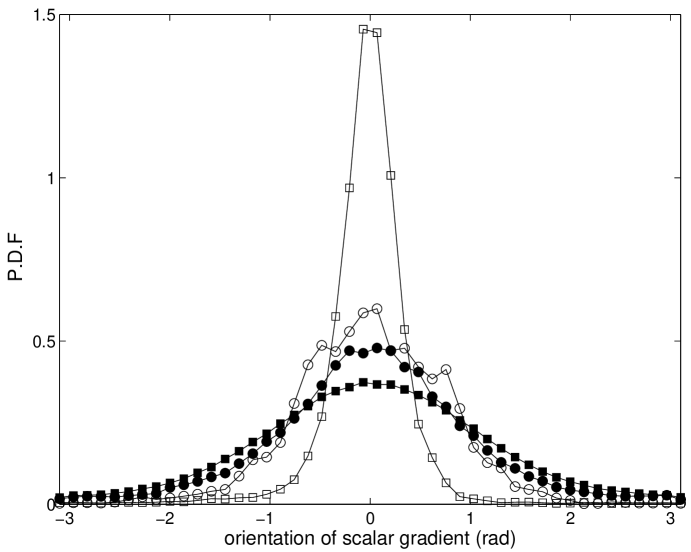
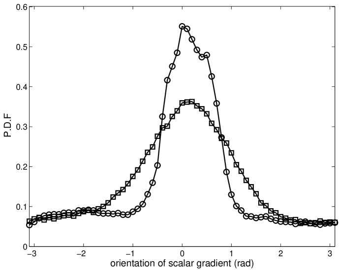
The p.d.f’s of scalar gradient alignment have been derived from the numerical evolution of computed using Eq. (3) and Eq. (2) with and . The fluctuations of thus describe the hyperbolic regime (), but also make significant inroads into the elliptic one (). The p.d.f’s of and conditioned on are shown in Fig. 1. They indicate which of the orientations (determined by the instantaneous value of ; Section 2.1) and (defined by ) is statistically the best one in the hyperbolic regime. Clearly, for the scalar gradient preferentially aligns with the instantaneous, equilibrium direction, , which is generally different from the compression one, in agreement with the approach by Lapeyre et al. [6]. For it is the alignment with the direction defined by which is the most probable one. Note that for and thus coincides with the compressional direction. Interestingly, in the present case the scalar gradient thus statistically aligns with the compressional direction because the gradient response to fluctuations is poor () and the mean value of corresponds to a pure hyperbolic regime (). This is reminiscent of the experimental situation analyzed by Garcia et al. [11].
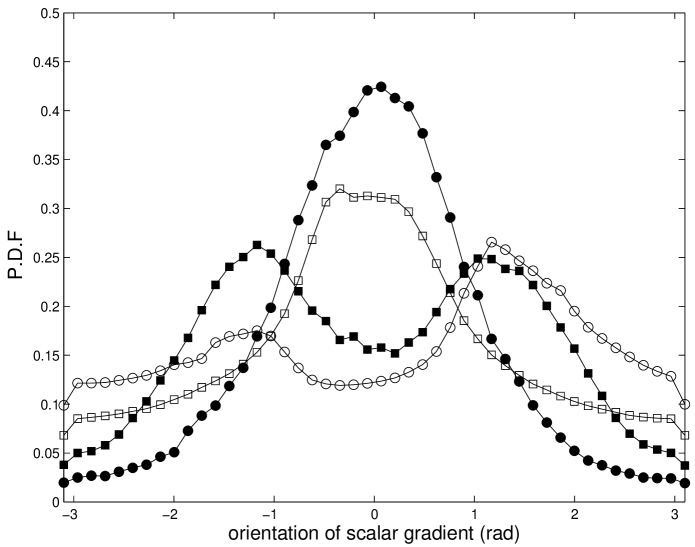
The results in the elliptic regime (p.d.f’s conditioned on ; Fig. 2) are similar. For the most probable gradient orientation is given by (Section 2.1) which agrees with the analysis of Lapeyre et al. [6]. In the case the scalar gradient again aligns preferentially with the direction defined by , that is, the compressional one. Yet this is not paradoxical. When the scalar gradient does not respond to the fluctuations of its orientation is governed by the mean value, , rather than by the instantaneous one and remains close to . This may drive the gradient to align with the compressional direction, even though takes elliptic values, provided that is close to zero. Note that the secondary maxima in Fig. 2 are explained by .
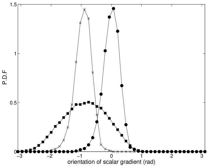
Alignment p.d.f’s derived with are plotted in Figs. 3 and 4. If is small the value of is immaterial; the scalar gradient preferentially aligns with the equilibrium direction, , and the same orientation p.d.f’s as those plotted in Figs. 1 and 2 for are derived. Figures 3 and 4 thus only display the orientation p.d.f’s in the case where is given a large value, . Results for the hyperbolic regime are presented in Fig. 3. Plainly, (which is computed as ) is the most probable orientation of the scalar gradient. Alignment with the equilibrium direction, , is weak and as shown by the p.d.f of there is no trend of the gradient to align with the compressional direction.
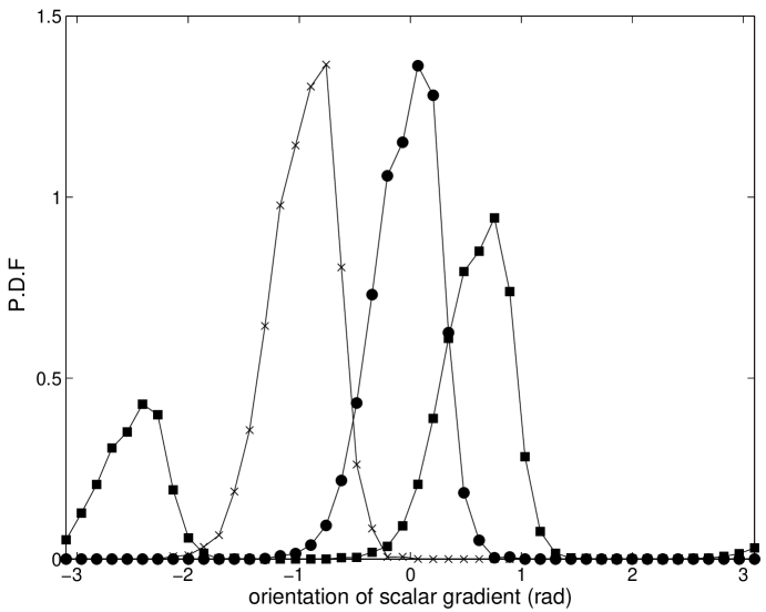
In the elliptic regime (Fig. 4), too, the orientation defined by is statistically the best one. As a matter of course, the gradient does not align with the compressional direction, but there is also no trend at all toward the direction defined by .
3 “Gradient production” and mixing properties
With the same assumptions as those stated in Section 2.1 the equation for the norm of the scalar gradient is [6, 9]
from which it is clear that the mean growth rate of the gradient norm, , is given by . Note that alignment with the compressional direction, , corresponds to the maximum growth rate.
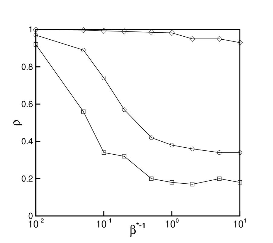
The mean growth rate has been derived from the statistics of computed by solving Eqs. (2) and (3). The simulations have been run for three different signals, namely , and with ranging from 0.1 to 100. For all cases .
Figure 5 shows the evolution of vs. . Interestingly, decreases with whatever the value of ; in other words, the better the response of gradient orientation to fluctuations (large values of ), the lower the mean growth rate of the norm. When it responds to fluctuations the scalar gradient preferentially aligns with either or which are determined by the instantaneous value of and are both mostly different from the compressional direction (Section 2.2). Hence the weaker growth rate. This feature gets more pronounced as the variance is increased. For the lowest variance () mostly fluctuates within the bounds of the hyperbolic regime assuming low values around and makes not much different from the compressional direction. Wider fluctuations ( or ), by contrast, bring about instantaneous orientations corresponding to larger values of and thus lying further from the compressional direction; in addition, more frequent, deep inroads into the elliptic regime () even lead the gradient to align with , that is, away from the compressional direction, during longer time intervals. As a result, for moderate and large values of the mean growth rate of the scalar gradient norm is lowered as the amplitude of fluctuations is increased. For the smallest values of , though, the growth rate is insensitive to variance and is close to its maximum value. Indeed a sluggish response to fluctuations compels the gradient to remain aligned with the direction defined by (Section 2.2) which in the present case (for which ) coincides with the compressional direction.
There is an interesting consequence for mixing properties. If , then favourable conditions for mixing are not only achieved in the hyperbolic regime; provided that the gradient response is weak, they are also fulfiled in those cases where large fluctuations of span both the hyperbolic and elliptic regimes. More generally, when fluctuates with remaining close to 0 it is the poor response of the scalar gradient to fluctuations that promotes the best conditions for fast mixing.
4 Analysis of experimental data on scalar gradient alignment
As far as we know, simultaneous measurements of velocity and scalar gradients are scarce. Apart from experiments in turbulent flows [14], joint statistics of velocity gradient and temperature gradient have been measured in a low-Reynolds number, two-dimensional, Bénard - von Kármán street [15, 16]. The latter data confirm that for fast fluctuations of strain persistence the preferential orientation of the scalar gradient is determined by the mean strain persistence rather than by its instantaneous value.
A detailed description of the experiment and measurement techniques are given in Refs. [15, 16, 17]. In brief, the experimental set-up consists of a 2 mm-diameter () circular cylinder used for generating a two-dimensional Bénard - von Kármán street; the Reynolds number based on the cylinder diameter is . Temperature is passively injected through a 20 m-diameter heated line source located in the near wake of the cylinder (Fig. 6). The line source can be set either in or off the centre of the street. Velocity gradients and temperature gradients are derived from simultaneous measurements of temperature and velocity components. These data have been used to obtain Lagrangian statistics of the scalar gradient orientation conditioned on the strain persistence parameter, , as explained in Refs. [7, 11].
Part of the latter results have been already analyzed [7, 11]. In particular, it has been found that in this experiment the temperature gradient does not respond to fluctuations. More precisely, , where the mean value of strain, , and , the autocorrelation time scale of , have been computed by averaging over Lagrangian trajectories. This previous statistical study was mainly focused on the hyperbolic zones of the flow, far enough downstream (i.e. with the distance of the source to the cylinder), when the heated line source is in the centre of the cylinder wake. The analysis showed (Fig. 7) that the alignment of the temperature gradient with the compressional direction is statistically better than with the equilibrium direction derived from the approach of Lapeyre et al. [6] (Section 2.1). This result lends support to the findings of the numerical study presented in Section 2.2. Most likely, preferential alignment of the temperature gradient with the compressional direction does not result from any kinematic attraction, but from the gradient dynamics. Because of the poor response of the temperature gradient to fluctuations, the preferential alignment is given by computed along Lagrangian trajectories which, in the above conditions, is found to be close to 0 and thus defines an orientation that almost coincides with the compressional direction.
Previous studies [9, 18] suggest that molecular diffusion may influence scalar gradient orientation, but that large gradients are weakly affected. As to the present case, Garcia et al. [11] have shown that the departure of the experimental results from the Lapeyre et al. approach is not to be ascribed to molecular diffusion. The latter certainly plays on the shape of the orientation p.d.f’s, but is not the cause for the compressional direction being more probable than the equilibrium one.
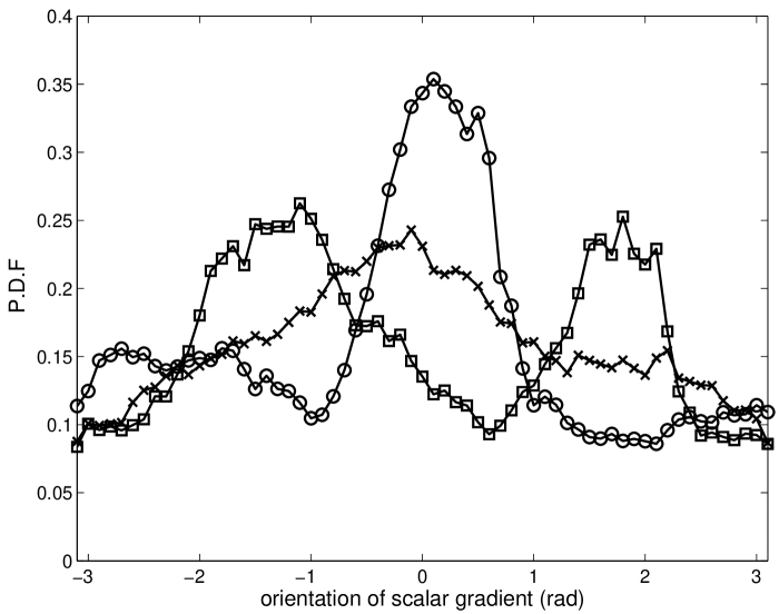
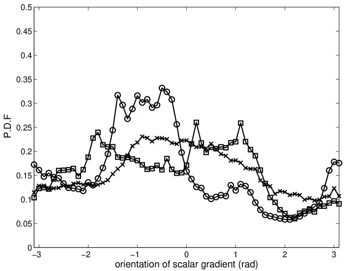
Further experimental data for the elliptic regions of the flow and in the case where the line source is located off the centre of the cylinder wake confirm the above picture. Results for elliptic regions when the line source is in the centre of the wake are displayed in Fig. 8. They concern the p.d.f’s of orientation of the temperature gradient with respect to the compressional direction, , and to direction imposed by dominating effective rotation [6] (Section 2.1). The p.d.f of orientation with respect to direction is also shown. The latter direction corresponds to the lowest eigenvalue of tensor which is defined as:
and is related to the pressure Hessian [10]. According to Klein et al. [10], when strain intensity varies significantly along Lagrangian trajectories is the preferential orientation of the scalar gradient in effective-rotation-dominated regions. From Fig. 8 it is clear that the temperature gradient does not tend to align with . There is a trend of the gradient to align with , but the best alignment is with the compressional direction. This striking behaviour strongly pleads for the above-described scenario and for the conclusions of the numerical analysis of Section 2.2: when strain persistence fluctuations are too fast for the scalar gradient to respond (which in the experiment is measured by the low value of ) the latter is blind to the local topology and its orientation is entirely governed by the mean value of the strain persistence parameter.
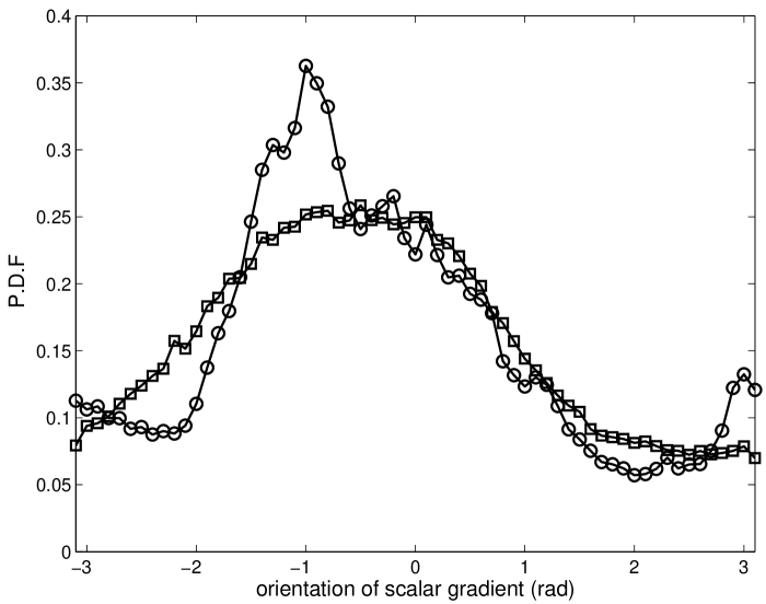
When the heated line source is set off the centre of the Bénard - von Kármán street (more precisely, at transversal distance from the previous position) the mean value of strain persistence computed for Lagrangian trajectories along which the temperature gradient keeps significant values () is found to be close to -0.8. Figure 9 shows the p.d.f’s of temperature gradient orientation with respect to either the compressional direction or the equilibrium direction, , derived from the approach of Lapeyre et al. [6], in strain-dominated regions. There is a trend of the gradient to align with . However, a much better statistical alignment is found with the direction corresponding to , that is, with . P.d.f’s of Fig. 9 are more distributed and thus display lower peaks than those corresponding to the source being in the centre of the cylinder wake (Fig. 7). This may result from a bigger influence of rotation on the temperature gradient when the line source is off the centre of the wake. Orientation statistics in effective-rotation-dominated regions have similar trends. Figure 10 shows that the temperature gradient aligns slightly better with than with . But in this case, too, the best statistical alignment – broader though the p.d.f is – is found around . These latter experimental data with thus give a more general support to the previous findings on the dynamics of scalar gradient orientation.
5 Conclusion
Analysis of the behaviour of the passive scalar gradient undergoing the influence of varying velocity derivatives through fluctuating strain persistence uncovers some interesting results regarding both the statistical gradient orientation and mixing properties.
Generalizing the analysis of Garcia et al. [11] to the effective-rotation-dominated regime, we confirm that the statistics of scalar gradient alignment depend on the gradient response to strain persistence fluctuations. More precisely, the numerical study based on the equation for the scalar gradient orientation in two-dimensional flow shows that perfect response drives the gradient to preferentially align with a direction determined by the instantaneous value of strain persistence as predicted by the analysis of Lapeyre et al. [6]. When the response of the scalar gradient is poor, though, the preferential alignment is given by the mean value of strain persistence which indicates whether the flow regime is, on an average, either strain- or effective-rotation-dominated. It follows interestingly that the scalar gradient preferentially aligns with the compressional direction provided that it is almost insensitive to strain persistence fluctuations and the mean strain persistence is close to the pure hyperbolic value. This result opposes the usual statement that it is a perfect response to the fluctuating rotation of the strain basis (which in the two-dimensional case is explicit in the strain persistence parameter) that leads the gradient to align with the compressional direction.
The general picture derived from the numerical study is firmly supported by experimental, Lagrangian joint statistics of velocity gradient and scalar gradient derived from simultaneous measurements of velocity and temperature in a two-dimensional, low-Reynolds number Bénard - von Kárman street. It is worth noting that its low Reynolds number marks this flow from the simulated two-dimensional turbulent flows in which scalar gradient alignment was previously studied [6, 9]. In particular, it may be that alignment with the equilibrium direction found by Lapeyre et al. [6] results from a good response of the scalar gradient to fluctuations in turbulent flows (moderate or large ). Checking this surmise would require Lagrangian data on strain persistence in two-dimensional turbulence. Regarding the Lagrangian properties of strain persistence and scalar gradient dynamics, another interesting and unanswered issue is whether the present flow is a special one or belongs to a more general class of flows.
Finally, unsteady behaviour of the scalar gradient may unexpectably affect mixing properties through alignment statistics. An interesting result is that poor response of the gradient to strain persistence fluctuations does not inevitably oppose efficient mixing. In particular, the study of the growth rate of the gradient norm clearly shows that when the mean strain persistence is close to the pure hyperbolic value (in other words, strain is persistent on an average) it is the weak response of the gradient to strain persistence fluctuations which promotes the highest growth rate and thus the best conditions for mixing.
Appendix A Behaviour of scalar gradient orientation for fast fluctuations of strain persistence
We restrict to the case where and is defined.
We get rid of the nonlinearity of Eq. (4) by assuming small values of . To first order, then:
| (5) |
with . The proof is thus not general, but is given as an additional argument for the behaviour of the scalar gradient when its response to fluctuations is poor.
We assume a sine signal for , , in which frequency is normalized as with . The nondimensional frequency, , thus gives a measure of the response of the scalar gradient to fluctuations. In particular, poor response is expected for large values of .
The solution of Eq. (5) is:
| (6) |
Note that Eq. (6) can be recast in the more standard form:
with and phase, , is present when the response to the stimulation is not perfect.
It follows that when fluctuates on a much shorter time scale than the response time scale of the scalar gradient so much so that the latter does not keep up with fluctuations the gradient orientation, , remains close to . Increasing the amplitude of fluctuations, however, leads to the opposite behaviour.
References
- [1] A. Pumir, Phys. Fluids 6, 2118 (1994).
- [2] W. D. Smyth, J. Fluid Mech. 401, 209 (1999).
- [3] P. Vedula, P. K. Yeung, R. O. Fox, J. Fluid Mech. 433, 29 (2001).
- [4] G. Brethouwer, J. C. R. Hunt, F. T. M. Nieuwstadt, J. Fluid Mech. 474, 193 (2003).
- [5] M. Tabor, I. Klapper, Chaos, Solitons Fractals 4, 1031 (1994).
- [6] G. Lapeyre, P. Klein, B. L. Hua, Phys. Fluids 11, 3729 (1999).
- [7] A. Garcia, Ph. D. thesis, University of Rouen, 2006.
- [8] A. Garcia, M. Gonzalez, Phys. Fluids 18, 058101 (2006).
- [9] G. Lapeyre, B. L. Hua, P. Klein, Phys. Fluids 13, 251 (2001).
- [10] P. Klein, B. L. Hua, G. Lapeyre, Physica D 146, 246 (2000).
- [11] A. Garcia, M. Gonzalez, P. Paranthoën, Phys. Fluids 17, 117102 (2005).
- [12] E. Dresselhaus, M. Tabor, J. Fluid Mech. 236, 415 (1991).
- [13] B. L. Hua, P. Klein, Physica D 113, 98 (1998).
- [14] B. Galanti, G. Gulitsky, M. Kholmyansky, A. Tsinober, S. Yorish, in Advances in Turbulence X, Proceedings of the 10th European Turbulence Conference, edited by H. I. Andersson and P.-Å. Krogstad, Trondheim, Norway, 2004.
- [15] G. Godard, Ph.D. thesis, University of Rouen, 2001.
- [16] G. Godard, M. Gonzalez, P. Paranthoën, in Advances in Turbulence IX, Proceedings of the 9th European Turbulence Conference, edited by I. P. Castro, P. E. Hancock and T. G. Thomas, Southampton, United Kingdom, 2002.
- [17] P. Paranthoën, G. Godard, F. Weiss, M. Gonzalez, Int. J. Heat Mass Transfer 47, 819 (2004).
- [18] P. Constantin, I. Procaccia, D. Segel, Phys. Rev. E 51, 3207 (1995).
FIGURE CAPTION
FIG. 1 P.d.f’s of scalar gradient orientation for and conditioned on (dominating strain). P.d.f of : , ; p.d.f of : , .
FIG. 2 P.d.f’s of scalar gradient orientation for and conditioned on (dominating effective rotation). P.d.f of : , ; p.d.f of : , .
FIG. 3 P.d.f’s of scalar gradient orientation for , and conditioned on (dominating strain). p.d.f of ; p.d.f of ; p.d.f of .
FIG. 4 P.d.f’s of scalar gradient orientation for , and conditioned on (dominating effective rotation). p.d.f of ; p.d.f of ; p.d.f of .
FIG. 5 Mean production rate of scalar gradient norm vs. . ; ; .
FIG. 6 Experimental set-up (from Godard [15]).
FIG. 7 Experimental p.d.f’s of temperature gradient orientation conditioned on (dominating strain) and in the far field of the heated line source (). The source is in the centre of the cylinder wake; experimental . p.d.f of ; p.d.f of .
FIG. 8 Experimental p.d.f’s of temperature gradient orientation conditioned on (dominating effective rotation) and in the far field of the heated line source (). The source is in the centre of the cylinder wake; experimental . p.d.f of ; p.d.f of ; p.d.f of .
FIG. 9 Experimental p.d.f’s of temperature gradient orientation conditioned on (dominating strain) and in the far field of the heated line source (). The source is off the centre of the cylinder wake (); experimental . p.d.f of ; p.d.f of .
FIG. 10 Experimental p.d.f’s of temperature gradient orientation conditioned on (dominating effective rotation) and in the far field of the heated line source (). The source is off the centre of the cylinder wake (); experimental . p.d.f of ; p.d.f of ; p.d.f of .
