Measurement of BAO correlations at $z=2.3$ with SDSS DR12 Ly$\alpha$-Forests

We have used flux-transmission correlations in Ly$\alpha$ forests to measure the imprint of baryon acoustic oscillations (BAO). The study uses spectra of 157,783 quasars in the redshift range $2.1\leq z\leq 3.5$ from the Sloan Digital Sky Survey (SDSS) Data Release 12 (DR12). Besides the statistical improvements on our previous studies using SDSS DR9 and DR11, we have implemented numerous improvements in the analysis procedure, allowing us to construct a physical model of the correlation function and to investigate potential systematic errors in the determination of the BAO peak position. The Hubble distance, $D_{H}=c/H(z)$, relative to the sound horizon is $D_{H}(z=2.33)/r_{d}=9.07\pm 0.31$. The best-determined combination of comoving angular-diameter distance, $D_{M}$, and the Hubble distance is found to be $D_{H}^{0.7}D_{M}^{0.3}/r_{d}=13.94\pm 0.35$. This value is $1.028\pm 0.026$ times the prediction of the flat-$\Lambda$CDM model consistent with the cosmic microwave background (CMB) anisotropy spectrum. The errors include marginalization over the effects of unidentified high-density absorption systems and fluctuations in ultraviolet ionizing radiation. Independently of the CMB measurements, the combination of our results and other BAO observations determine the open-$\Lambda$CDM density parameters to be $\Omega_{M}=0.296\pm 0.029$, $\Omega_{\Lambda}=0.699\pm 0.100$ and $\Omega_{k}=-0.002\pm 0.119$.

1 Introduction

The sound waves that propagated in the pre-recombination universe produced a pronounced peak in the two-point correlation function of the cosmological-density field (Peebles & Yu, 1970; Sunyaev & Zeldovich, 1970). This “baryon-acoustic oscillation” (BAO) peak, first observed by Eisenstein et al. (2005) and Cole et al. (2005), is centered on a comoving distance equal to the sound horizon at the drag epoch, $r_{d}$. Observed at a redshift $z$, the BAO peak position in the transverse (angular) direction determines the ratio $D_{M}(z)/r_{d}$, where $D_{M}(z)=(1+z)D_{A}(z)$ is the “comoving” angular-diameter distance ($D_{A}$ is the “traditional” angular-diameter distance). In the radial (redshift) direction, the peak position determines $D_{H}(z)/r_{d}$, where $D_{H}(z)=c/H(z)$ is the Hubble distance. Since $D_{M}$, $D_{H}$ and $r_{d}$ all have simple dependencies on the cosmological parameters, observation of the BAO feature constrains those parameters, especially when combined with cosmic microwave background (CMB) data (Planck Collaboration et al., 2014, 2016; Aubourg et al., 2015). In particular, one can constrain models beyond the flat-$\Lambda$CDM model that describes CMB data, deriving constraints on cosmological curvature and the dark-energy equation of state. Furthermore, the shape of the spectrum of CMB anisotropies can be used to calculate the value of $r_{d}$ to percent-level precision, $r_{d}\sim 147$ Mpc and the use of this value allows one to derive $D_{M}(z)$ and $D_{H}(z)$ from BAO measurements. These absolute distances can be combined with relative distances determined with type Ia supernovae (Betoule et al., 2014), to extrapolate to $z=0$, yielding a “top-down” measurement of $H_{0}$ (Aubourg et al., 2015).

Most studies of the BAO peak have used galaxies at redshifts $z<0.8$ as tracers of the density. The first observations used $z\sim 0.35$ data from the Sloan Digital Sky Survey (SDSS) (Eisenstein et al., 2005) and $z\sim 0.2$ data from the Two-Degree Field Redshift Survey (Cole et al., 2005), and the combination of these sets (Percival et al., 2007, 2010). Since then, results of increasingly higher precision have been obtained, most significantly in the redshift range $0.35<z<0.65$ from the Baryon Oscillation Spectroscopy Survey (BOSS) of SDSS-III (Anderson et al., 2012, 2014b, 2014a) with the results of the complete survey being summarized in Alam et al. (2016). Results at other redshifts have been obtained by 6dFGRS at $z\sim 0.11$ (Beutler et al., 2011), WiggleZ at $0.4<z<0.8$ (Blake et al., 2011), SDSS-I at $z\sim 0.35$ (Padmanabhan et al., 2012; Mehta et al., 2012; Chuang & Wang, 2012; Xu et al., 2013) and SDSS-I at $z\sim 0.15$ (Ross et al., 2015). There is an impressive agreement of the results of these studies with the expectations of flat-$\Lambda$CDM models based on CMB data, as emphasized by Planck Collaboration et al. (2016).

At higher redshifts, BAO correlations can be seen using quasars and their Lyman-$\alpha$ (Ly$\alpha$) forests as mass tracers (McDonald & Eisenstein, 2007). The correlations in the Ly$\alpha$-forest flux-transmission field of BOSS quasars were first studied in Slosar et al. (2011) and the BAO peak was seen in SDSS data release DR9 (Busca et al., 2013; Slosar et al., 2013; Kirkby et al., 2013) and DR11 (Delubac et al., 2015). Cross-correlations of the Ly$\alpha$ absorption with the distribution of quasars were detected in DR9 (Font-Ribera et al., 2013), and the first BAO detection was presented in Font-Ribera et al. (2014).

In this paper, we study the auto-correlation function, $\xi$, of the Ly$\alpha$ flux-transmission field using the SDSS data release DR12 and we update the cosmological constraints reported in Delubac et al. (2015). Our study of the quasar-forest cross-correlation function will be presented in a future publication (du Mas des Bourboux et al., in preparation). In addition to using the $15\%$ increase of survey area of DR12 over DR11, the following improvements over the analysis of Delubac et al. (2015) have been implemented:

• Spectroscopic pipeline improvements (Sect. 2) that includes a new algorithm for the extraction of spectra from the CCD images that results in a more linear flux response. This modification allows us to correct for the mean distortion of the flux-transmission field due to imperfect spectral modeling of standard stars. We also correct for the differential positioning of quasar and stellar fibers in the focal plane due to optimization at different wavelengths (Margala et al., 2016).

• The use of mock spectra with improved modeling of metal absorbers (Sect. 3), including both Ly$\alpha$-metal and metal-metal correlations.

• Modeling of the distortions of the correlation function due to quasar-continuum fitting (Sect. 4). This allows us to construct a physical model of the correlation function over the range $10<r<200\leavevmode\nobreak\ h^{-1}{\rm Mpc}$.

• Modeling of spurious correlations introduced by the pipeline (Sect. 5), calculation of their effect on the correlation function, and searches for unidentified spurious correlations using the Carbon-IV (CIV) forest, $142.0<\lambda_{\rm RF}<152.0$ nm.

• Fits of the data (Sect. 6) that marginalize over the contributions to the correlation function of metals, unidentified high-column-density systems, and fluctuations of ionizing UV flux.

None of these improvements induce significant changes in the derived values of $D_{H}/r_{d}$ and $D_{M}/r_{d}$; the differences (Sect. 8) with those of Delubac et al. (2015) are consistent with statistical fluctuations induced by the increased sample size.

This paper is organized as follows. Section 2 describes the DR12 data used in this analysis. Section 3 gives a brief description of the mock spectra used to test the analysis procedure, with a more detailed description being found in Bautista et al. (2015). Section 4 presents our method of estimating the flux-transmission field, its correlation function, and the associated covariance matrix. Section 5 studies spurious correlations induced by the pipeline. In Section 6 we fit the mocks and data to derive the BAO peak position parameters, $D_{M}(z=2.33)/r_{d}$ and $D_{H}(z=2.33)/r_{d}$. Section 7 investigates possible systematic errors in the measurement. In Section 8 we compare our measured peak position with the predictions of $\Lambda$CDM models and derive constraints on the associated cosmological parameters. Section 9 presents a brief summary.

Figure 1: SDSS DR12 footprint (in J2000 equatorial coordinates) used in this work. The survey covers one quarter of the sky ($10^{4}{\rm deg^{2}}$). The light blue regions are those added beyond the area covered by our previous study (Delubac et al., 2015). The dotted line is the Galactic plane.

Figure 2: Example of a BOSS quasar spectrum of redshift 2.91 (smoothed to the width of analysis pixels). The red and blue lines cover the forest region used in our analysis, $104.0<\lambda_{\rm RF}<120.0$ nm. This region is sandwiched between the quasar’s Ly$\beta$ and Ly$\alpha$ emission lines, respectively at 400.9 and 475.4 nm (restframe 102.572 and 121.567 nm). The blue line is the model of the continuum, $C_{q}(\lambda)$; the red line is the product of the continuum and the mean transmission, $C_{q}(\lambda)\times\overline{F}(z)$, as calculated by the method described in Sect. 4.

Figure 3: Weighted redshift distribution of pairs of Ly$\alpha$ forest pixels. The mean is $\langle z\rangle=2.33$. Included in the distribution are the $\sim 5\times 10^{10}$ pairs within $20\leavevmode\nobreak\ h^{-1}{\rm Mpc}$ of the center of the BAO peak.

2 The BOSS quasar sample and data reduction

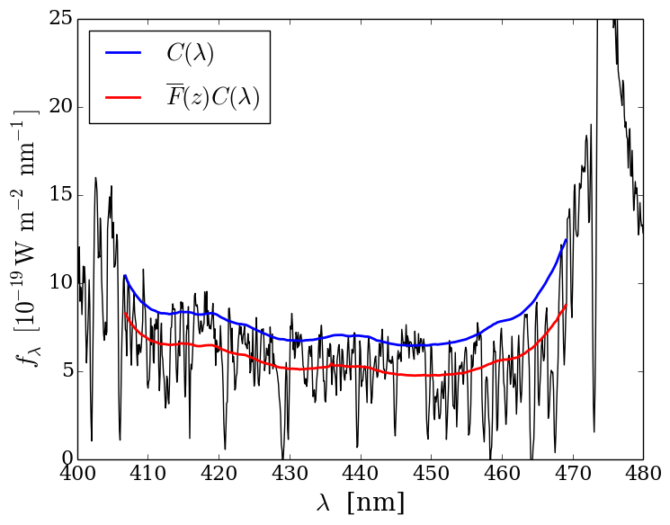
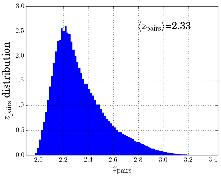
The quasar sample was gathered over a five-year period by the SDSS-III Collaboration (Eisenstein et al., 2011; Gunn et al., 1998, 2006; Smee et al., 2013). We use the data from the twelfth Data Release (DR12) of SDSS as presented in Alam et al. (2015). The associated quasar catalog is described in Pâris et al. (2016). Most of the quasar spectra were obtained by the Baryon Oscillation Spectroscopic Survey, BOSS (Dawson et al., 2013), but DR12 also includes six months of data from the SEQUELS program. The DR12 celestial footprint covering $\sim\pi\leavevmode\nobreak\ \rm{sr}\sim 10^{4}\leavevmode\nobreak\ {\rm deg^{2}}$ is displayed in Fig. 1. An example of a quasar spectrum in the Ly$\alpha$-forest region is shown in Fig. 2. The redshift distribution of measurement pairs in the forest is shown in Fig. 3.

The quasar target selection used in BOSS, summarized in Ross et al. (2012), combines different targeting methods described in Yèche et al. (2010), Kirkpatrick et al. (2011), and Bovy et al. (2011). The selection algorithms use SDSS photometry and, when available, data from the GALEX survey (Martin et al., 2005) in the UV; the UKIDSS survey (Lawrence et al., 2007) in the NIR, and the FIRST survey (Becker et al., 1995) in the radio.

The DR12 data were processed using a new software package that differs from the standard DR12 SDSS-III pipeline (Bolton et al., 2012) and which has become the standard pipeline for SDSS DR13 (SDSS Collaboration et al., 2016). For each object, both pipelines provide a flux calibrated spectrum, $f(\lambda)$, errors, and an object classification (galaxy, quasar, star). A model spectrum is fit to $f(\lambda)$ providing a redshift estimate. For this study, we use the “coadded” spectra constructed from typically four exposures of 15 minutes resampled at wavelength pixels of width $\Delta\log_{10}\lambda=10^{-4}$ ($c\Delta\lambda/\lambda\sim{\rm 69\leavevmode\nobreak\ km\,s^{-1}}$). For the small number of quasars with repeated observations, the coadded spectra can include exposures widely separated in time.

An important difference with respect to the DR12 pipeline is that pixels on the CCD image are combined to give a flux $f(\lambda)$ with pixel-weights determined only by the CCD readout noise. While this method is sub-optimal because it ignores photo-electron Poisson noise, compared to the DR12 method it yields an unbiased estimate of $f(\lambda)$ since the weights do not depend on the observed CCD counts which are needed to estimate Poisson noise. A more detailed description of the changes to the extraction pipeline is given in Appendix A.

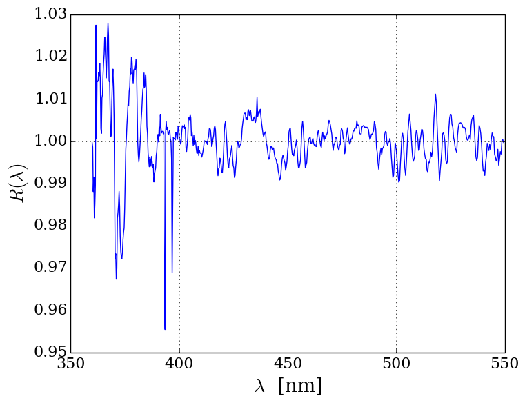
The ratio of observed flux to model flux, averaged over all spectra, is an important diagnostic of pipeline systematic errors. Figure 4 shows the average ratio, $R(\lambda)$, as a function of observed wavelength for quasar spectra on the red side of Ly$\alpha$ emission. Since model imperfections for individual quasar spectra are averaged over in this figure (because of the range of quasar redshifts), the deviations from unity reflect imperfections in the spectrograph flux calibration. The figure reveals percent-level deviations that are mostly due to imperfect modeling of photo-spectroscopic standard stars. The calcium H and K lines from interstellar absorption are also visible. In the analysis to be presented here, the $f(\lambda)$ are divided by $R(\lambda)$ to correct on average for these artifacts. This procedure is effective only with the fluxes from the DR13 pipeline since the non-linearities present in the DR12 pipeline make the correction flux-dependent. We show in Section 5 that after this global correction, remaining calibration artifacts (due to their time-dependence) are sufficiently small to have a negligible effect on the measurement of the correlation function.

The spectra of all quasar targets were visually inspected (Pâris et al., 2012, 2014, 2016) to correct for misidentifications, to flag broad absorption lines (BALs), and to establish the definitive quasar redshift. Damped Ly$\alpha$ troughs (DLAs) were visually flagged, but also identified and characterized automatically (Noterdaeme et al., 2012). The visual inspection of DR12 confirmed 297,301 quasars, of which 181,719 are in the redshift range appropriate for this study, 2.1 $\leq$ $z_{q}$ $\leq$ 3.5. We discarded quasars with visually identified BALs (to avoid the necessity of modeling their profiles in the forest) leaving 160,868 quasars. A further cut requiring a minimum number of unmasked forest pixels (50 “analysis pixels”; see below) yielded a sample of 157,922 quasars. Finally, 139 spectra failed the continuum-fitting procedure (Sect. 4.1), leaving 157,783 spectra compared to 137,562 in the Delubac et al. (2015) investigation.

For the measurement of the flux transmission, we use the rest-frame wavelength interval

$$104.0\,<\lambda_{\rm RF}<120.0\leavevmode\nobreak\ {\rm nm}\;.$$ (1)

As illustrated in Fig. 2, this range is bracketed by the emission lines $\lambda_{\rm Ly\beta}=102.572$ nm and $\lambda_{\rm Ly\alpha}=121.567$ nm. This region was chosen as the maximum range that avoids the large pixel variances on the slopes of the two lines due to quasar-to-quasar diversity of line-emission strength and profile. The absorber redshift, $z=\lambda/\lambda_{\rm Ly\alpha}-1$, is required to lie in the range $1.96<z<3.44$. The lower limit is set by the requirement that the observed wavelength be greater than 360 nm, below which the system throughput is less than 10% of its peak value. The upper limit is produced by the maximum quasar redshift of 3.5, beyond which the BOSS surface density of quasars is not sufficient to be useful for this study. The weighted distribution of redshifts of absorber pairs near the BAO peak position is shown in Fig. 3. The distribution has a mean of $\overline{z}=2.33$.

For the determination of the correlation function, we use analysis pixels that are the inverse-variance-weighted flux average over three adjacent pipeline pixels. Throughout the rest of this paper, “pixel” refers to analysis pixels unless otherwise stated. The width of these pixels is $207\leavevmode\nobreak\ {\rm km\leavevmode\nobreak\ s^{-1}}$ corresponding at $z\sim 2.33$ to an observed-wavelength width $\sim 0.28\leavevmode\nobreak\ {\rm nm}$ and a comoving radial distance of $\sim 2.0\leavevmode\nobreak\ h^{-1}{\rm Mpc}$. The total sample of 157,783 spectra thus provides $\sim 3\times 10^{7}$ measurements of Ly$\alpha$ absorption over an effective volume of $\sim 50\leavevmode\nobreak\ {\rm Gpc}^{3}$.

Figure 4: Mean ratio, $R(\lambda)$, of observed flux to pipeline-model flux as a function of observed wavelength for quasar spectra to the red of the Ly$\alpha$ emission line ($\lambda_{\rm RF}>130\leavevmode\nobreak\ {\rm nm}$). (The mean is calculated by weighting each measurement by the inverse of the pipeline variance.) In this mostly unabsorbed region of quasar spectra, the percent-level wavelength-dependent deviations from unity are due to imperfect modeling of calibration stars and to the calcium H and K lines (393.4 and 396.9 nm) due to Galactic absorption.

Figure 5: One-dimensional flux-correlation function, $\xi_{\rm 1d}$, for BOSS quasars showing correlations of $\delta_{q}(\lambda)$ within the same forest. The correlation function is shown as a function of wavelength ratio for the data and for the mocks (procedure Met1). Prominent peaks due to Ly$\alpha$-metal and metal-metal correlations are indicated. The peak at $\lambda_{1}/\lambda_{2}\sim 1.051$, which is seen in the data but not in the mocks, is due to CII(133.5)-SiIV(140.277) at $z\sim 1.85$, outside the redshift range covered by the mocks.

Table 1: Parameters of the flat $\Lambda$CDM cosmological model used for the production and analysis of the mock spectra and the CMB-based flat $\Lambda$CDM model from Planck Collaboration et al. (2016) used for the analysis of the data. The models are defined by the cold dark matter, baryon, and massive neutrinos densities, the Hubble constant, the number of light neutrino species, and the inhomogeneity parameters, $\sigma_{8}$ and $n_{s}$. The sound horizon, $r_{d}$, is calculated using CAMB (Lewis et al., 2000).

	Mocks	Planck
		(TT+lowP)
$\Omega_{M}h^{2}$	0.1323	0.1426
$=\Omega_{C}h^{2}$	0.1096	0.1197
$\;+\Omega_{B}h^{2}$	0.0227	0.02222
$\;+\Omega_{\nu}h^{2}$	0	0.0006
$h$	0.7	0.6731
$N_{\nu}$	3	3
$\sigma_{8}$	0.795	0.829
$n_{s}$	0.97	0.9655
$\Omega_{M}$	0.27	0.3147
$r_{d}$ [Mpc]	149.7	147.33
	(104.80 $h^{-1}$)	(99.17 $h^{-1}$)
$D_{M}(2.33)/r_{d}$	38.63	39.15
$D_{H}(2.33)/r_{d}$	8.744	8.612

3 Mock quasar spectra

In order to test the analysis procedure and investigate statistical and possible systematic errors, we created 100 sets of mock spectra that reproduce the essential physical and instrumental characteristics of the BOSS spectra. The basic method for the production of the mocks with Ly$\alpha$ absorption is described in Font-Ribera et al. (2012). Except for the implementation of absorption due to metals and high column-density systems (HCDs, i.e., damped Ly$\alpha$-systems and Lyman-limit systems), the mocks used in this study are identical to the DR11 mocks (Bautista et al., 2015) that were used in Delubac et al. (2015). The DR11 mocks therefore cover $\sim 15\%$ less solid angle than the DR12 data.

For each set of spectra, the background quasars were assigned the angular positions and redshifts of the DR11 quasars. The unabsorbed spectra (continua) of the quasars were generated using the Principal Component Analysis eigenspectra of Suzuki et al. (2005). The amplitudes for each eigenspectrum were randomly drawn from Gaussian distributions with a dispersion equal to that of the corresponding eigenvalues in Table 1 of Suzuki (2006). The overall normalization was chosen by fitting the mock spectrum to the corresponding observed spectrum.

The Ly$\alpha$ absorption field was generated using the technique described in Font-Ribera et al. (2012) in which a Gaussian random field, $\delta_{G}$, is first defined at the positions of the $\sim 10^{7}$ observed forest pixels. Flux transmissions were defined by the non-linear transformation

$$F(\delta_{G})=\exp\left[-a(z)e^{b(z)\delta_{G}}\right].$$

The two functions, a(z) and b(z) are chosen so that the resulting mean transmission and variance are near those observed in the data. The correlations of the field $\delta_{G}$ are chosen so that the correlations of $F(\delta_{G})$ follow the linear correlations of the “mock” cosmology of Table 1 modified by non-linear effects (McDonald, 2003). For pixels randomly distributed in space, this procedure would involve inverting a $10^{7}\times 10^{7}$ matrix. To reduce the problem to a manageable size, use was made of the fact that the forest pixels are nearly parallel, allowing a separate treatment of radial and transverse coordinates.

In the final step, the spectra were modified to include the effects of the BOSS spectrograph point spread function (PSF), readout noise, photon noise, and flux systematic errors.

For each of the 100 mock data sets, four types of spectra were produced and analyzed. The first type consists simply of Ly$\alpha$ flux-transmission fraction, $F_{\rm Ly\alpha}(\lambda)$, modified for the wavelength resolution but without multiplication by a quasar continuum spectrum, $C(\lambda)$. Analysis of this mock type allowed us to study the recovery of the BAO peak position under the most favorable conditions. With the introduction of the quasar continuum, the second type consists of more realistic spectra, $F_{\rm Ly\alpha}(\lambda)C(\lambda)$. Analysis of this type tests our ability to fit the quasar continuum and to model the resulting distortion of the correlation function.

The final two types of spectra add to $F_{\rm Ly\alpha}(\lambda)$ absorption that is due to HCDs and to metals. Following Font-Ribera & Miralda-Escudé (2012), HCDs are placed at randomly chosen pixels where the optical depth was above a chosen threshold. The neutral-hydrogen column densities were drawn randomly with $N_{\rm HI}>10^{17.2}\leavevmode\nobreak\ {\rm cm^{-2}}$, assuming an intrinsic power-law distribution corrected for self-shielding and normalized to match the observations of Prochaska et al. (2005). Because the HCDs are placed in redshift space, the resulting HCDs have correlations that trace the underlying density field but with a redshift-space distortion parameter that is not necessarily equal to that of physical HCDs.

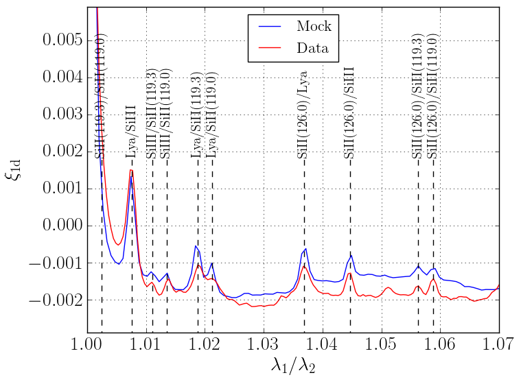
Absorption due to metal transitions was also simulated by adding absorption in proportion to the Ly$\alpha$ absorption at the same redshift. The important transitions can be seen in the “one dimensional” correlation function, $\xi_{\rm 1d}(\lambda_{1}/\lambda_{2})$ for fluxes at two wavelengths within the same forest, as shown in Fig. 5. In this figure, the peaks correspond to absorption by two different transitions by material at the same physical position but a different wavelength. The most prominent features are due to pairs comprising Ly$\alpha$ and one metal transition, but there are also features due to metal-metal pairs. More detailed information can be obtained by stacking spectra around strong absorbers in the forest (Pieri et al., 2010, 2014). Table 2 lists the transitions included in the mock spectra.

We have tested two procedures for adding metal absorption to the primary Ly$\alpha$ absorption. The methods are defined by the assumed relation between Ly$\alpha$ absorption and metal absorption at the same physical position. For each wavelength, $\lambda$, with Ly$\alpha$ absorption $A_{\rm Ly\alpha}(\lambda)=1-F_{\rm Ly\alpha}(\lambda)$, an appropriate metal absorption $A_{m}(\lambda+\Delta\lambda_{m})$ for each transition, $m$, is chosen. A simple procedure would be to choose $A_{m}\propto A_{\rm Ly\alpha}$ with a proportionality constant chosen to reproduce the Ly$\alpha$-metal features in the observed $\xi_{\rm 1d}$. However, this procedure does not produce significant features corresponding to metal-metal correlations. To do this it is necessary to add, for a randomly chosen small fraction of wavelengths, a much larger metal absorption.

The first procedure (hereafter Met1) aims to match the observed line-of-sight correlation function $\xi_{\rm 1d}$, in particular the amplitudes of the peaks associated to Ly$\alpha$-metal and metal-metal correlations. We first transform the pure mock Ly$\alpha$ flux into “optical depth” $\tau_{\rm Ly\alpha}$ and define the metal absorption of transition $m$ as $\tau_{m}=a_{m}\tau_{\rm Ly\alpha}$. A quadratic term in $\tau_{\rm Ly\alpha}$ is added for a fraction of the strong Ly$\alpha$ absorbers to simulate strong metal absorption. The parameters $a_{m}$, the quadratic terms and rates of strong absorption are set to match the observed amplitudes in the data $\xi_{\rm 1d}$.

The second procedure (hereafter Met2) aims to match the observed stack of high signal-to-noise ratio Ly$\alpha$ absorbers, while maintaining consistency with the $\xi_{\rm 1d}$ in the resulting mock $\xi_{\rm 1d}$. Following Pieri et al. (2014), stacks were produced using the DR12 Ly$\alpha$ forest sample. As a function of the Ly$\alpha$ transmission, we measured amplitudes for the metal absorption features. The obtained “flux decrements” caused by metals were treated as target average flux decrements. Metals are implemented in Met2 mocks as a mix of weak and strong metal absorption, generating a mock $\xi_{\rm 1d}$ consistent with the observed $\xi_{\rm 1d}$ and consistent with the absorption frame measurements of Pieri et al. (2014).

The metal absorption added by these methods is due to the presence of metals at the same physical position as HI. Because our mocks provide the HI density only for redshifts $z>1.9$, we cannot generate absorption at lower redshifts that nevertheless appears in the Ly$\alpha$ forest because of transition wavelengths much greater than that of Ly$\alpha$. An important example is CIV doublet ($\overline{\lambda}=154.9$ nm) where the absorption at an observed wavelength of 400 nm is due to material at $z\sim 1.6$. Fortunately this absorption has little effect on the correlation function, as we will see in Sect. 6.

The statistical properties of metal absorption in the mocks are determined by the underlying density field. However, the analysis procedure interprets absorption at a given wavelength as absorption due to the Ly$\alpha$ transition. Because of this behavior, the metal contribution to the measured correlation function is shifted and deformed in $(r_{\perp},r_{\parallel})$ space. In particular, the large correlation due to HI and metals at the same physical position is seen at $(r_{\perp}\sim 0,r_{\parallel})$ with $r_{\parallel}=(1+z)D_{H}(z)\Delta\lambda/\lambda$ where $\Delta\lambda/\lambda$ is the relative wavelength separation of the metal feature with respect to Ly$\alpha$. This leads to a large correlation at this $r_{\parallel}$ (and $r_{\perp}\sim 0$), so if the amplitude is significant, it can be measured. Table 2 lists the apparent $r_{\parallel}$ corresponding to vanishing Ly$\alpha$-metal separation.

Table 2: Transitions contributing to absorption by metals in the mock spectra. The second column shows $r_{\parallel}=(1+\bar{z})D_{H}(\bar{z})(\lambda_{met}-\lambda_{\rm Ly\alpha}/)\lambda$, the reconstructed separation corresponding to correlations of Ly$\alpha$ and metal absorption at the same physical position.

transition	$r_{\parallel}$ [$h^{-1}{\rm Mpc}$]
SiIII(120.7 nm)	21
SiIIa(119.0 nm)	64
SiIIb(119.3 nm)	56
SiIIc(126.0 nm)	111

Figure 6: Mean transmission, $\overline{F}(\lambda)$, calculated using the DR12 pipeline of our previous investigations, and using the DR13 pipeline applied to DR12 data of this analysis. The DR13 pipeline allows us to divide forest spectra by the correction factor (Fig. 4) derived from the spectra on the red side of Ly$\alpha$ emission. This procedure eliminates most of the small scale structure found with the old pipeline that is due to artifacts of stellar modeling, Galactic calcium H and K absorption, and sky lines.

4 Measurement of flux-transmission field and its correlation function

In this Section we describe the measurement of the correlation function of the transmitted flux fraction:

$$\delta_{q}(\lambda)=\frac{f_{q}(\lambda)}{C_{q}(\lambda)\overline{F}(z)}-1\;\;.$$ (2)

Here, $f_{q}(\lambda)$ is the observed flux density for quasar $q$ at observed wavelength $\lambda$, $C_{q}(\lambda)$ is the unabsorbed flux density (the so-called “continuum”) and $\overline{F}(z)$ is the mean transmitted fraction at the absorber redshift, $z(\lambda)=\lambda/\lambda_{\rm Ly\alpha}-1$. Measurement of the flux-transmission field $\delta_{q}(\lambda)$ requires estimates of the product $C_{q}(\lambda)\overline{F}(z)$ for each quasar. An example is shown in Fig. 2. The estimation procedures, described in this Section, differ slightly from those of our previous studies (Busca et al., 2013; Delubac et al., 2015). One important modification is that we now calculate the distortion of the correlation function due to continuum-fitting (Sect. 4.3).

4.1 Estimation of $\delta_{q}(\lambda)$

As in our previous investigations, we assume the quasar continuum, $C_{q}(\lambda)$, is the product of a universal function of the rest-frame wavelength, $\lambda_{\rm RF}=\lambda/(1+z_{q})$, and a linear function of $\log\lambda$, included to account for quasar spectral diversity:

$$C_{q}(\lambda)=C(\lambda_{\rm RF})(a_{q}+b_{q}\log(\lambda))$$ (3)

with $C(\lambda_{\rm RF})$ being normalized so that its integral over the forest is equal to unity. The $(a_{q},b_{q})$ and $C(\lambda_{\rm RF})$ are determined by maximizing the likelihood function given by

$$L=\prod_{q,\lambda}P(\,f_{q}(\lambda)\;|\;C_{q}(\lambda)\,)\;.$$ (4)

Here $P(f_{q}(\lambda)\,|\,C_{q}(\lambda))$ is the probability to observe a flux $f_{q}(\lambda)$ for a given continuum found by convolving the intrinsic probability, $D(F=f_{q}(\lambda)/C_{q}(\lambda),z)$, with the observational resolution assumed to be Gaussian:

$$P(\,f_{q}(\lambda)\;|\;C_{q}(\lambda)\,)\propto\int_{0}^{1}dFD(F,z)\exp\left[\frac{-(C_{q}F-f_{q}(\lambda))^{2}}{2\sigma_{q}(\lambda)^{2}}\right]\;.$$ (5)

Here, $\sigma_{q}(\lambda)^{2}$ is the variance due to readout noise and photon statistics.

A continuum-determination method is defined by the assumed form of $D(F,z)$. For this work, it is taken to be the log-normal model of absorption used to generate the mock data, corresponding to “method 2” of our previous studies (Delubac et al., 2015). As a check, we also use “method 1”, which is equivalent to using a narrow Gaussian for $D(F,z)$, thereby producing only the product $C_{q}(\lambda)\overline{F}(\lambda)$ for each forest.

In practice, we maximize the likelihood iteratively by assuming a $C(\lambda_{\rm RF})$ to determine the $(a_{q},b_{q})$. The mean absorption $\overline{F}(\lambda)$ is then calculated by an appropriately weighted average of $f_{q}(\lambda)/C_{q}(\lambda)$ (for fixed $\lambda$) after which $C(\lambda_{\rm RF})$ is recalculated as an average of $f_{q}(\lambda)/\overline{F}(z)$ (for fixed $\lambda_{\rm RF}$). The procedure is stopped after ten iterations, at which point a stability of $\sim 10^{-4}$ is reached for $C(\lambda_{\rm RF})$ and $\overline{F}(\lambda)$. Figure 2 shows a spectrum with its $C_{q}(\lambda)$ and $C_{q}\overline{F}$.

The function $\overline{F}(z)$ to be used in Eq. 2 to calculate $\delta_{q}(\lambda)$ is the mean of $f_{q}(\lambda)/C_{q}(\lambda)$ and can thus differ slightly from $\overline{D(F,z)}$ used in the model to estimate the $C_{q}(\lambda)$. The use of the mean of $f_{q}(\lambda)/C_{q}(\lambda)$ ensures that the mean of $\delta$ is zero at each redshift (or wavelength).

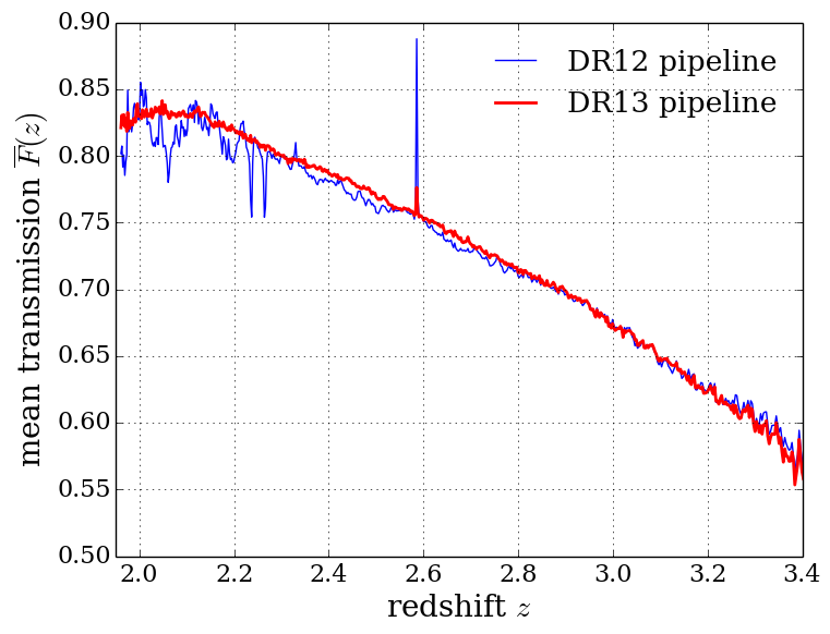
Figure 6 displays the calculated $\overline{F}(z)$, both for the DR13 pipeline used here and the DR12 pipeline used previously. The use of the new pipeline removes most of the artifacts in the old analysis. We emphasize, however, that the derived $\overline{F}(z)$ is dependent on the assumed form of $D(F,z)$ and should therefore not be considered as a measurement of the mean absorption. For example, the flattening of $\overline{F}(z)$ for $z<2.1$ ($\lambda<377\leavevmode\nobreak\ {\rm nm}$) suggests that we have slightly underestimated $\overline{F}(z)$ at these redshifts. Since, by construction, the mean $\delta$ vanishes at each redshift, this implies that our procedure makes a compensating overestimate of the $C_{q}(\lambda)$. Since it is the product $\overline{F}(z)C_{q}(\lambda)$ that determines $\delta_{q}(\lambda)$, the measured correlation function is therefore not strongly affected.

Those forests with identified DLAs are given a special treatment. All pixels where the absorption due to the DLA is higher than 20% are not used. The absorption in the wings is corrected using a Voigt profile following the procedure of Noterdaeme et al. (2012).

We denote as $\tilde{\delta}_{q}(\lambda)$ the estimate of $\delta_{q}(\lambda)$ using the relation (2). Because forest data is used to fit for $C_{q}(\lambda)$ and $\overline{F}(z)$ the measured $\tilde{\delta}_{q}(\lambda)$ is not equal to the original $\delta_{q}(\lambda)$. We can identify two effects. First, the use of $\overline{F}(\lambda)$ is equivalent to the transformation

$$\tilde{\delta}_{q}(\lambda)=\delta_{q}(\lambda)-\overline{\delta(\lambda)}$$ (6)

where the over-bar refers to the average over forests at fixed $\lambda$. Second, the fitting of $(a_{q},b_{q})$ with the data biases toward zero the mean $\tilde{\delta}_{q}(\lambda)$ and mean $(\log\lambda-\overline{\log\lambda})\tilde{\delta}_{q}(\lambda)$. To simplify this effect and facilitate its correction we explicitly subtract the mean and first moment for each forest

$$\hat{\delta}_{q}(\lambda)=\tilde{\delta}_{q}(\lambda)-\overline{\tilde{\delta}_{q}}-(\Lambda-\overline{\Lambda_{q}})\frac{\overline{(\Lambda-\overline{\Lambda_{q}})\tilde{\delta}}}{\overline{(\Lambda-\overline{\Lambda_{q}})^{2}}}\hskip 14.22636pt\Lambda\equiv\log\lambda$$ (7)

where the over-bars refer to averages within a given forest using the weights defined in the next Section. The accompanying distortion of the correlation function is non-negligible, as we will demonstrate in Sect. 6.2 with the mock spectra.

The transformation (7) has two interesting effects on the measured flux-transmission field. Most importantly, it makes it simple to calculate the distortion of the correlation function (Sect. 4.3) and thus simplifies the relation between the underlying physical model and the measured correlation function. Second, it nearly eliminates the difference between the correlations functions calculated with the two continuum fitting methods used in Delubac et al. (2015) with the r.m.s. difference in the two $\xi(r_{\perp},r_{\parallel})$ being 0.056 of the r.m.s. uncertainty per $(r_{\perp},r_{\parallel})$ bin.

4.2 Estimation of the correlation functions

For the estimator of the flux auto-correlation function, we adopt a simple weighted sum of products of the $\hat{\delta}$:

$$\hat{\xi}_{A}=\frac{\sum_{ij\in A}w_{i}w_{j}\hat{\delta}_{i}\hat{\delta}_{j}}{\sum_{ij\in A}w_{i}w_{j}}\;,$$ (8)

where the $w_{i}$ are weights (see below) and each $i$ (or $j$) indexes a measurement on a quasar $q_{i}$ at wavelength $\lambda_{i}$. The sum over $(i,j)$ is understood to run over all pairs of pixels within a bin $A$ in the space of pixel separations, $(A)\rightarrow(r_{\perp},r_{\parallel})$. We exclude pairs of pixels from the same quasar to avoid the correlated errors in $\hat{\delta}_{i}$ and $\hat{\delta}_{j}$ arising from the estimate of $C_{q}(\lambda)$ for the spectrum of the quasar. The bins $A$ are defined by a range of width $4\leavevmode\nobreak\ h^{-1}{\rm Mpc}$ of the components perpendicular and parallel to the line of sight, $r_{\perp}$ and $r_{\parallel}$. We use 50 bins in each component, spanning the range from $0$ to $200\leavevmode\nobreak\ h^{-1}{\rm Mpc}$; the total number of bins used for evaluating the correlation function is therefore 2500. Separations in observational pixel coordinates (RA,Dec,$\lambda$) are transformed to $(r_{\perp},r_{\parallel})$ in units of $h^{-1}{\rm Mpc}$ by assuming that absorption is due to the Ly$\alpha$ transition and using the cosmological parameters from Table 1 (Planck cosmology for the data and the mock cosmology for the mocks).

As described in Delubac et al. (2015), the weights, $w_{i}$, are chosen so as to account for both Poisson noise in the flux measurement and for the intrinsic fluctuations in $\hat{\delta}_{i}$ due to cosmological large-scale structure. The weights are set to zero for pixels flagged by the pipeline as having problems due, for example to sky emission lines or cosmic rays. To reduce the pipeline systematics discussed in Sect. 5, we also do not use pairs of pixels that have nearly the same wavelength ($r_{\parallel}<4\leavevmode\nobreak\ h^{-1}{\rm Mpc}$) and that were taken on the same exposures.

4.3 The distortion matrix

The transformations (6) and (7) mix pixels so that the correlation $\langle\hat{\delta}_{q}(\lambda)\hat{\delta}_{q^{\prime}}(\lambda^{\prime})\rangle$ is equal to the original $\langle\delta_{q}(\lambda)\delta_{q^{\prime}}(\lambda^{\prime})\rangle$ plus a linear combination of the correlations of other pixel-pairs $\langle\delta_{q^{\prime\prime}}(\lambda^{\prime\prime})\delta_{q^{\prime\prime\prime}}(\lambda^{\prime\prime\prime})\rangle$. This approach means that the measured correlation function $\hat{\xi}$ is a “distorted” version of the true correlation function $\xi$. Since the transformations (6) and (7) are linear, the relation between measured and true correlation functions is given by a distortion matrix $D_{AB}$:

$$\hat{\xi}_{A}=\sum_{B}D_{AB}\xi_{B}$$ (9)

where $A$ and $B$ refer to bins in pixel separation space. Writing $\hat{\delta}_{i}=\sum_{i^{\prime}}\eta_{ii^{\prime}}\delta_{i^{\prime}}$ produces

$$D_{AB}=w_{A}^{-1}\sum_{i,j\in A}w_{i}w_{j}\left[\sum_{i^{\prime},j^{\prime}\in B}\eta_{ii^{\prime}}\eta_{jj^{\prime}}\right]$$ (10)

where $w_{A}=\sum_{i,j\in A}w_{i}w_{j}$. We ignore the small effect of transformation (6), in which case $\eta_{ii^{\prime}}=0$ unless the pixels $i$ and $i^{\prime}$ are in the same forest:

$$\eta_{ii^{\prime}}=\delta_{ii^{\prime}}-\frac{w_{i^{\prime}}}{\sum_{k}w_{k}}-\frac{(\Lambda_{i}-\overline{\Lambda})w_{i^{\prime}}(\Lambda_{i^{\prime}}-\overline{\Lambda})}{\sum_{k}w_{k}(\Lambda_{k}-\overline{\Lambda})^{2}}\hskip 14.22636pt\Lambda=\log\lambda$$ (11)

where the two sums over $k$ include only pixels in the same forest as that of $i$ and $i^{\prime}$ and the over-bars refer to averages in that forest. The matrix $D_{AB}$ thus depends only on the geometry and weights of the survey. We will see its effect on the mock correlation function in Sect. 6.2 (Fig. 11).

Previous analyses (Busca et al., 2013; Slosar et al., 2013; Delubac et al., 2015; Blomqvist et al., 2015) have dealt with the distortions introduced by continuum-fitting in different ways. Busca et al. (2013) and Delubac et al. (2015) model it as an additive power law in $r$ and $\mu$ with 12 free parameters. Blomqvist et al. (2015) assumed that continuum-fitting reduces the observed amplitude of long-wavelength modes in the direction parallel to the line of sight. They then model it as a multiplicative function of $k_{\parallel}$ that tends to zero at large scales (with $k_{\parallel}\lesssim 2\pi/L$, where $L\sim 380\leavevmode\nobreak\ h^{-1}{\rm Mpc}$ is the typical length of a forest) and to one at small scales ($k_{\parallel}\gg 2\pi/L$). They tune the shape of the function using simulated data to ultimately reduce the number of free parameters to one.

In our approach we do not introduce free parameters to account for the effects of continuum-fitting. Instead, we follow the assumption, first proposed by Slosar et al. (2013), that at each line of sight the continuum-fit delta field differs from the true delta field by a linear function in $\Lambda$. Slosar et al. (2013) then de-weight these “linear modes” in their covariance matrix. Alternatively, we use the transformation from $\delta$ to $\hat{\delta}$ to remove the “linear modes” from the model via the distortion matrix.

Figure 7: Correlation, $Corr_{AB}=C_{AB}/\sqrt{C_{AA}C_{BB}}$, plotted vs. $\Delta r_{\parallel}=|r_{\parallel}^{A}-r_{\parallel}^{B}|$ for the two lowest intervals of $\Delta r_{\perp}=|r_{\perp}^{A}-r_{\perp}^{B}|$. The correlation is averaged over $(r_{\perp}^{B},r_{\parallel}^{B})$. The left panel is the Metal (Met1) mocks and the right panel is for the data. As labeled, the correlation is calculated by subsampling (eqn. 13), by assuming “independent forests” (eqn. 14, offset by $0.5h^{-1}{\rm Mpc}$ for clarity), or by the mock-to-mock variation (eqn. 15). Good agreement between the methods is seen, though the independent-forest method necessarily underestimates the correlation for $\Delta r_{\perp}\neq 0$. The differences between the mocks and the data reflect the differences in $\xi_{\rm 1d}$ (Fig. 5).

4.4 The covariance matrix

The covariance matrix associated with $\hat{\xi}$ is:

$$C_{AB}=\frac{1}{W_{A}W_{B}}\sum_{ij\in A}\sum_{kl\in B}w_{i}w_{j}w_{k}w_{l}[\langle\hat{\delta}_{i}\hat{\delta}_{j}\hat{\delta}_{k}\hat{\delta}_{l}\rangle-\langle\hat{\delta}_{i}\hat{\delta}_{j}\rangle\langle\hat{\delta}_{k}\hat{\delta}_{l}\rangle]$$ (12)

where $W_{A}=\sum_{ij\in A}w_{i}w_{j}$. Following Delubac et al. (2015), we evaluate $C_{AB}$ by dividing the BOSS footprint into sub-samples and measuring $\xi^{s}_{A}$ and $\xi^{s}_{B}$ in each sub-sample $s$. Neglecting the small correlations between sub-samples, and replacing the four-point function by the measured product of correlations in subsamples, the covariance is given by

$$C_{AB}=\frac{1}{W_{A}W_{B}}\sum_{s}W_{A}^{s}W_{B}^{s}[\hat{\xi}^{s}_{A}\hat{\xi}^{s}_{B}-\hat{\xi}_{A}\hat{\xi}_{B}]\;,$$ (13)

where the $W_{A}^{s}$ are the sums of weights in the sub-sample $s$. As in Delubac et al. (2015), the SDSS plates define the sub-samples.

As a check of the subsampling method, the sum (12) can also be estimated by neglecting inter-forest correlations, in which case the four-point function vanishes unless the four pixels are drawn from just two spectra:

$$C_{AB}=\frac{1}{W_{A}W_{B}}\sum_{ij\in A}\sum_{kl\in B}w_{i}w_{j}w_{k}w_{l}\xi_{\rm 1d}(\lambda_{i}/\lambda_{k})\xi_{\rm 1d}(\lambda_{j}/\lambda_{l})$$ (14)

The sum can then be estimated from a random sample of forest pairs. Because neighboring forests are nearly parallel, the sum necessarily gives $C_{AB}=0$ unless $r_{\perp}^{A}\sim r_{\perp}^{B}$.

Finally, for the analysis of the mock data, the covariance matrix can also by calculated from the mock-to-mock variations of $\xi$:

$$C_{AB}=\overline{\hat{\xi}_{A}\hat{\xi}_{B}}-\overline{\hat{\xi}_{A}}\;\overline{\hat{\xi}_{B}}\;,$$ (15)

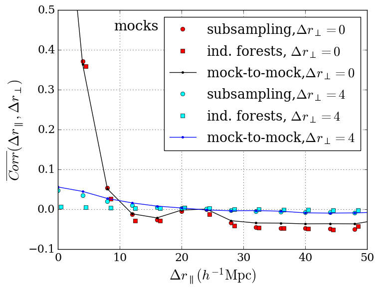
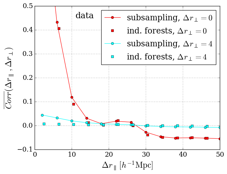
where the over-bar refers to averages over the set of 100 mocks. Given the approximations used in the calculation of $C_{AB}$ via eqns. 13 or 14, it is of great importance that the mock-to-mock variations confirm the accuracy of the other two methods when applied to mock data. This comparison is shown in Fig. 7.

The $2500\times 2500$ element matrix, $C_{AB}$, has a relatively simple structure. By far the most important elements are the diagonal elements which are, to good approximation, inversely proportional to the number of pixel pairs used in the calculation of the correlation function; the number of pairs is roughly proportional to $r_{\perp}$:

$$C(r_{\perp},r_{\parallel},r_{\perp},r_{\parallel})\;\sim\;\frac{0.043}{N_{pairs}}\sim\frac{2.5\times 10^{-10}}{r_{\perp}/100\leavevmode\nobreak\ h^{-1}{\rm Mpc}}\;.$$ (16)

The variance is about twice as large as what one would calculate assuming all (analysis) pixels used to calculate $\xi(r_{\perp},r_{\parallel})$ are independent. This decrease in the effective number of pixels is due to the physical and instrumental correlations between neighboring pixels in a given forest (eqn. 14).

The off-diagonal elements of the covariance matrix also have a simple structure. As previously noted, the covariance is mostly due to the two-forest part of the four-point function which, because neighboring forests are nearly parallel, only contribute to the covariance matrix elements with $r_{\perp}=r_{\perp}^{\prime}$. This behavior is illustrated in Fig. 7, which displays the mean values of the correlation matrix elements as a function of $r_{\parallel}-r_{\parallel}^{\prime}$ for the smallest values of $r_{\perp}-r_{\perp}^{\prime}$.

The statistical precision of the sub-sampling calculation is $\sim 0.02$ for individual elements of the correlation matrix. Figure 7 reveals that only correlations with $\Delta r_{\perp}\sim 0$ and $\Delta r_{\parallel}<20\leavevmode\nobreak\ h^{-1}{\rm Mpc}$ are greater than the statistical precision and therefore sufficiently large for individual matrix elements to be measured accurately by sub-sampling. As in Delubac et al. (2015), we therefore average the sub-sampling correlation matrix over $(r_{\perp}^{\prime},r_{\parallel}^{\prime})$ and use the resulting covariance matrix that is a function of $(r_{\perp}-r_{\perp}^{\prime},r_{\parallel}-r_{\parallel}^{\prime})$.

5 Correlations introduced by the optics and data pipeline

Spurious correlations in $\delta_{q}(\lambda)$ are introduced by the telescope and spectrometer optics, and by the pipeline reductions of the data. These correlations are superimposed on the physical $\xi(r_{\perp},r_{\parallel})$ that we wish to measure; in this Section we estimate the various contributions.

5.1 Optical cross-talk

At the optical level, correlations are introduced by signals from one object “scattering” into the spectra of other objects, that is through optical cross-talk. There is negligible cross-talk introduced in the telescope focal plane by photons from one object entering into the fiber of another object. However, there can be measurable cross-talk between neighboring fibers downstream of the wavelength dispersion where they are focused on the CCD. This contamination arises through imperfect modeling of the point-spread function when transforming the two-dimensional CCD image into a series of one-dimensional spectra, $f(\lambda)$. We have measured the cross-talk as a function of fiber separation by fitting the signal in sky fibers to a sky model and a weighted sum of the spectra of the objects (quasars or galaxies) in neighboring fibers. Consistent with the results of Croft et al. (2016), we find the cross-talk for the neighboring fibers is $\sim 0.2\%$ and $\sim 0.05\%$ for fibers separated by two or three rows respectively, and is consistent with zero for larger separations.

The cross-talk directly introduces correlations between pixels at the same wavelength but these pixel pairs are, at any rate, not used in the analysis. The cross-talk introduced between pixels $\lambda_{1}$ and $\lambda_{2}$ of two quasars is proportional to the product of the cross-talk amplitude and to $\xi_{\rm 1d}(\lambda_{1}/\lambda_{2})$. We have verified that these correlations are insignificant compared to the measured $\xi$. This fact is in part due to the fiber-assignment strategy which avoided placing two quasar candidates on neighboring fibers.

5.2 Pipeline-induced correlations

The pipeline treatment of the spectrometer data transforms flat-field corrected CCD counts, $f_{q}^{\rm m}(\lambda)$, to fluxes, $f_{q}(\lambda)$. This process requires subtracting a sky contribution, $B_{q}(\lambda)$, and multiplying by a calibration vector, $A_{q}(\lambda)$, that corrects for the wavelength-dependent throughput of the system:

$$f_{q}(\lambda)=A_{q}(\lambda)\;[f_{q}^{\rm m}(\lambda)-B_{q}(\lambda)]\;.$$ (17)

Both $A_{q}(\lambda)$ and $B_{q}(\lambda)$ are determined from spectra taken simultaneously with the data: spectra of spectro-photometric standard stars for $A_{q}$, and spectra of “sky fibers” (fibers pointing to empty sky regions) for $B_{q}$. The spectra from the 1000 fibers of a given exposure are treated independently for the two 500-fiber spectrographs because of possible differential variations of instrumental properties such as throughput, PSF, and scattered light. (See Smee et al. (2013) for the relevant details of the spectrometer construction.) Hereafter, the collection of fibers of a given plate assigned to one of the two spectrographs will be referred to as a “half-plate.” Inaccuracies in the determinations of $A_{q}$ and $B_{q}$ will lead directly to correlated inaccuracies in the $f_{q}(\lambda)$ of a given half-plate.

Errors in the sky subtraction, $B_{q}(\lambda)$, are simple to model because they are mostly due to well-understood Poisson fluctuations of photo-electron counts in the $\sim 50$ sky fibers per half-plate. The pipeline interpolates these measurements in the focal plane to produce the sky background to be subtracted from a given quasar. The limited number of sky-fibers results in correlations between $f_{q}(\lambda)$ and $f_{q^{\prime}}(\lambda^{\prime})$ for $q\neq q^{\prime}$ and $\lambda=\lambda^{\prime}$ since the sky subtractions where calculated using the same noisy sky-fibers. These correlations for $\lambda=\lambda^{\prime}$ generate small correlations for $\lambda\neq\lambda^{\prime}$ through continuum fitting, as discussed in Sect. 4.2. Because the correlations are primarily for $\lambda=\lambda^{\prime}$ they contribute a spurious $\xi(r_{\perp},r_{\parallel}=0)$ for pairs of pixels on the same half-plate.

Errors on the calibration vector $A_{q}$ are also Poissonian in that they are due to the fluctuations in the imperfect modeling of $\sim 10$ calibration stars per half-plate. The mean over all spectra of the imperfections are visible in the mean “transmission” of the unabsorbed parts of quasar spectra shown in Fig. 4. As mentioned in Section 2, the mean imperfections are removed by dividing forest spectra by $R(\lambda)$ from Fig. 4. However, fluctuations from exposure to exposure remain because of the spectral variations of the small number of calibration stars used. The statistical properties of these variations have been estimated by comparing the $A_{q}$ measured with random sub-samples of stars and, independently, by comparing the $A_{q}$ on different half-plates for the same exposure. Unlike the correlations due to sky-subtraction, which are confined to $\lambda=\lambda^{\prime}$, the errors in the calibration vectors are strongly correlated over the characteristic wavelength range of stellar spectral features, $\Delta\lambda\sim 1$ nm.

We constructed a model for pipeline-induced correlations that uses the measured statistical properties of the $A_{q}(\lambda)$ and $B_{q}(\lambda)$. The contribution of the sky noise was estimated using a fit of random realizations of the signal in the sky fibers (using a degree 2 polynomial fit as a function of the fiber number). The realizations were based on the statistical uncertainty estimation from the pipeline (which we have found to be accurate at the 5% level, see Fig. 19, bottom panel). A normalization factor was applied to account for the average difference of calibration between the sky and target fibers (a $\sim 10\%$ correction). Performing a fit allowed us to capture accurately the resulting correlations as a function of fiber separation.

The contribution of the calibration was estimated using the fact that because the flux calibration of the two spectrographs is determined independently, the difference of those two calibration solutions for each exposure provides us with an estimate of their statistical fluctuation (up to a normalization factor $\sqrt{2}$) while retaining the correlation of those fluctuations as a function of wavelength. Those differences for all DR12 plates was computed. Their average per observation run was subtracted in order to account for the actual difference of throughput of the two spectrographs and their evolution during the course of the survey. This data set provided us with a library of calibration uncertainties that was used to calculate calibration-induced correlations between spectra.

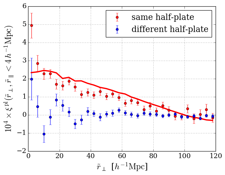
This model was used to calculate the expected correlation between pixels in the Ly$\alpha$ forest of one quasar and pixels in the CIV forest ($142<\lambda_{\rm RF}<152$ nm) of another quasar. The physical correlation of the two forests is due mostly to the auto-correlation of the weak CIV absorption in the two forests, but any pipeline-induced correlations should be present at full strength. Since this cross-correlation is designed to isolate pipeline-induced effects, we denote this correlation function as $\xi^{\rm pl}(\lambda_{2}-\lambda_{1},\theta)$ where $(\lambda_{1},\lambda_{2})$ are the wavelengths in the two forests and $\theta$ is the angular separation. We also distinguish between $\xi^{\rm pl}$ and correlations between flux pairs on the same half-plate, $\xi^{\rm pl}({hp=hp^{\prime}})$, and correlations between flux pairs on different half-plates, $\xi^{\rm pl}({hp\neq hp^{\prime}})$. While these correlations are naturally given as a function of wavelength and angular separations, for convenience, the $\xi^{\rm pl}$ will be given as functions of pseudo-separations $(\tilde{r}_{\perp},\tilde{r}_{\parallel})$ calculated using the Ly$\alpha$ rest-frame wavelength to define redshifts in both spectra. With this approach, $\tilde{r}_{\parallel}=0$ corresponds to absorption at the same observed wavelength.

This correlation for same-half-plate pairs (measured using the techniques of Sect. 4.2) is shown with the red points in Fig. 8 for the first $\tilde{r}_{\parallel}$ bin ($\tilde{r}_{\parallel}<4\leavevmode\nobreak\ h^{-1}{\rm Mpc}$). Superimposed on the data is the prediction of the model of the pipeline-induced correlations. For the first $\tilde{r}_{\parallel}$ bin, the correlation is dominated by those induced by to the sky-subtraction model. There is good agreement between this simple model and the observed correlations.

The pipeline-induced correlations that we have considered do not contribute to correlations between pixels observed on different half-plates. The different-half-plates correlation functions for the $\tilde{r}_{\parallel}<4\leavevmode\nobreak\ h^{-1}{\rm Mpc}$ bin is shown by the blue points in Fig. 8. The correlations for different half-plates (blue points) are clearly far less than those for same half-plates (red points). For $\tilde{r}_{\parallel}<4\leavevmode\nobreak\ h^{-1}{\rm Mpc},\tilde{r}_{\perp}<\leavevmode\nobreak\ 60\leavevmode\nobreak\ h^{-1}{\rm Mpc}$, $\chi^{2}=28.6$ ($N_{\rm dof}=15$) for the no-correlation hypothesis.

For the $\tilde{r}_{\parallel}>4\leavevmode\nobreak\ h^{-1}{\rm Mpc}$ bins, the model predicts much smaller correlations. In particular, the sky-subtraction model noise induces non-zero correlations only because of the continuum fit which distorts the original correlation function as described in Section 4.2. This behavior is illustrated in Fig. 9 showing $\xi^{\rm pl}$ in four ranges of $\mu$. Because of the low level of absorption fluctuations redward of Ly$\alpha$ emission, the variance of the points is a factor $\sim 7$ smaller than the corresponding variance for the forest-forest correlation function.

Figure 8: Correlation between pixels in the Ly$\alpha$-forest and pixels in the CIV-forest, $\xi^{\rm pl}(\lambda_{2}-\lambda_{1},\theta)$ for small wavelength differences. The wavelength difference and angular separation have been transformed to pseudo-separations $(\tilde{r}_{\perp},\tilde{r}_{\parallel}<4\leavevmode\nobreak\ h^{-1}{\rm Mpc})$ assuming Ly$\alpha$ absorption in both forests. The red points show the correlation for pairs on the same halfplate $\xi^{\rm pl}_{hp=hp^{\prime}}(\tilde{r}_{\perp},\tilde{r}_{\parallel}<4\leavevmode\nobreak\ h^{-1}{\rm Mpc})$. The much smaller correlations for different half-plates are the blue points. The red line represents the prediction for our model of calibration and sky noise.

Figure 9: Null test for pipeline-induced correlations. As in Fig. 8, the correlation between the Ly$\alpha$-forest pixels and the CIV-forest pixels, $\xi^{\rm pl}(\tilde{r}_{\parallel},\tilde{r}_{\perp})$ is shown, but now for four angular ranges as labeled and offset by 0.1 successively for clarity. Pixel pairs with $\tilde{r}_{\parallel}<4\leavevmode\nobreak\ h^{-1}{\rm Mpc}$ are excluded. There is no evidence for pipeline-induced systematics with the $\chi^{2}$ for vanishing correlation for $12<\tilde{r}<160\leavevmode\nobreak\ h^{-1}{\rm Mpc}$ is $(32.5,\,31.2,\,22.7,\,40.0)$ for the four ranges, each with 38 data points.

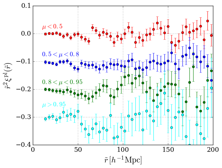
The model for pipeline-induced correlations assumes that the sky-subtraction errors are entirely due to Poisson statistics of photo-electron counts, neglecting possible wavelength- and position-dependent systematic mis-estimates of the sky flux. While the changes applied to the pipeline (Appendix A) considerably reduced the systematic sky residuals, significant residuals remain on bright sky lines due to an imperfect PSF model, PSF variations and displacement of spectral traces (due to changes of temperature and variations of the gravity load of the spectrographs which are at the Cassegrain focus of the telescope). We tested the effect of those sky residuals by computing the correlation function of fake Ly$\alpha$ forests consisting of the residual signal in the nearest sky fiber in the CCD divided by the quasar continuum model (we made sure to use only once each sky fiber in this process to avoid introducing an artificial correlation). The measured correlation signal could be entirely explained by the Poissonian sky model noise described above. We hence conclude that the systematic sky residuals induce a negligible contamination to the Ly$\alpha$ correlation function.

This analysis presented above evaluates the contamination due to any additive signal to the Ly$\alpha$ forest that leads to a correlated signal in the CCD. It includes the systematic sky residuals, their fluctuations from plate to plate, but also the potential effect of scattered light in the spectrograph.

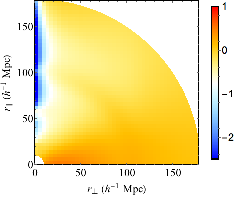
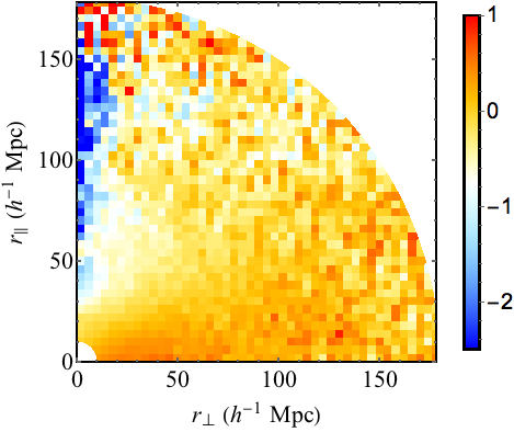
We have used our model of pipeline-induced correlations to calculate their effect on the determination of the BAO peak position. Since the model contains no scale near the BAO scale, it is not surprising that it predicts no measurable influence, as reported in Table 7 of Sect. 7. Furthermore, to facilitate the comparison of the measured correlation function with the physical model developed in the next section, we do not use pairs of pixels on the same exposure that would contribute to the $r_{\perp}<4\leavevmode\nobreak\ h^{-1}{\rm Mpc}$ bins of $\xi(r_{\perp},r_{\parallel})$.

Figure 10: Two-dimensional representation of $r^{2}\xi(r_{\perp},r_{\parallel})$ in units of $(h^{-1}{\rm Mpc})^{2}$. The right panel shows the measurement and the left panel the best-fit model, $\xi^{\rm ph}$, modified by the distortion matrix via eqn. (18). The BAO feature is at $r\sim 100\leavevmode\nobreak\ h^{-1}{\rm Mpc}$. The effects of metal-Ly$\alpha$ correlations are seen in the lowest $r_{\perp}$ bin, in particular the peak at $50<r_{\parallel}<70\leavevmode\nobreak\ h^{-1}{\rm Mpc}$ due to SiIIa and SiIIb.

Table 3: Parameters of the physical model for the correlation function and their best-fit values for the data fit over the range $10<r<180\leavevmode\nobreak\ h^{-1}{\rm Mpc}$. The parameters include the BAO peak-position parameters, $(\alpha_{\perp},\alpha_{\parallel})$, the bias parameters $(b,\beta)$ at redshift $z=2.3$ for the various components, the length scale, $L_{\rm HCD}$, for unidentified HCDs, and the bias parameter, $b_{\Gamma}$ for UV fluctuations. The biases $b_{\rm HCD}$ and $b_{\Gamma}$ are relative to $b_{\rm Ly\alpha}$. Parameters without uncertainties are fixed in the fit. These include the UV absorber response bias, $b_{a}^{\prime}$, the UV attenuation length, $\lambda_{\rm UV}$, the BAO amplitude parameter, $A_{\rm peak}$, the bias redshift-evolution parameter, $\gamma$, and the peak-broadening parameters $\@vec{\Sigma}$.

parameters	best fit	best fit
$\alpha_{\parallel},\alpha_{\perp}$	$1.053\pm 0.036$	$0.965\pm 0.055$
$b(1+\beta),\beta\;$ Ly$\alpha$	$-0.325\pm 0.004$	$1.663\pm 0.085$
$b,\beta\;$ Si3	$-0.0033\pm 0.0013$	$0.500$
$b,\beta\;$ Si2a	$-0.0044\pm 0.0009$	$0.500$
$b,\beta\;$ Si2b	$-0.0035\pm 0.0009$	$0.500$
$b,\beta\;$ Si2c	$-0.0015\pm 0.0012$	$0.500$
$b,\beta\;$ CIV	$-0.0233\pm 0.0114$	$0.500$
$b,\beta\;$ HCDs	$-0.0288\pm 0.0043$	$0.681\pm 0.175$
$L_{\rm HCD}$	$24.3410\pm 1.1308$
$b_{\Gamma},\,b^{\prime}_{a}$	$0.1125\pm 0.0512$	$-2/3$
$\lambda_{\rm UV}[h^{-1}{\rm Mpc}]$	$300.00$
$A_{\rm peak}$	$1.00$
$\gamma$	$2.90$
$\Sigma_{\perp},\Sigma_{\parallel}\;$	$3.26$	$6.41$

6 Fits for the BAO peak position

To determine the position of the BAO peak in the transverse and radial directions, we fit the measured $\xi(r_{\perp},r_{\parallel})$ to functions that describe the underlying large-scale-structure correlations. These correlations are primarily due to Ly$\alpha$ absorption in the intergalactic medium (IGM), but we also include absorption by metals in the IGM and neutral hydrogen in high-column-density systems (HCDs). The physical correlations are corrected for distortions that are introduced by the procedure for determining the quasar continuum (Sect. 4.3). The fitting routine we use gives results consistent with those found using the publicly available baofit package (Kirkby et al., 2013; Blomqvist et al., 2015) modified to include the effects described in this Section. The parameters of the fits are described below and in Table 3. The best-fit model correlation function is shown in Fig. 10.

Figure 11: Correlation function for the metal-free mocks in four ranges of $\mu$. The black points and curves correspond to mocks with Ly$\alpha$ absorption but without the addition of a quasar continuum. The red points and curves correspond to mocks with the addition of a continuum. The points correspond to stacks of 100 mocks and the light curves to individual mocks. The heavy curves correspond to the input model of Table 1 (after distortion by the matrix $D_{AA^{\prime}}$ (eqn. 10) for the red curve).

Figure 12: Correlation function for the stack of the 100 mocks in four ranges of $\mu$. The red points represent the measured correlation function of the mocks with metals and the red curves shows the best fit. The black points indicate the correlation function after including, in addition to metals, HCDs unmasked for $N_{\rm HI}<10^{20}{\rm cm^{-2}}$ and the black curve the best fit. The peak at $r\sim 60\leavevmode\nobreak\ h^{-1}{\rm Mpc}$ due to SiIIa and SiIIb is apparent in the range $\mu>0.95$ but not in the range $0.8<\mu<0.95$.

Figure 13: Measured $\alpha_{\perp}$ and $\alpha_{\parallel}$ (left) and $\beta_{\rm Ly\alpha}$ and $b_{\rm Ly\alpha}(1+\beta_{\rm Ly\alpha})$ (right) for the 100 mock catalogs including HCDs with $N_{\rm HI}>10^{20}{\rm cm^{2}}$ masked. There are four outliers on the left plot and two on the right. The horizontal and vertical blue lines show the weighted means of the distributions, also given in Table LABEL:fitmocktable. The distribution and mean values of $(\alpha_{\perp},\alpha_{\parallel})$ indicates no significant bias in the reconstruction of the BAO peak-position parameters.

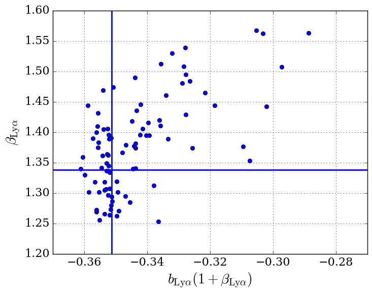
6.1 The model of the correlation function

The general form for the model correlation function $\xi_{A}$ of the $(r_{\perp},r_{\parallel})$ bin $A$ is a distorted sum of the cosmological, or “physical” correlation function, $\xi^{\rm ph}_{A}$, and a slowly varying function, $B_{A}$, used to test for systematics:

$$\xi_{A}=\sum_{A^{\prime}}D_{AA^{\prime}}\left[\xi^{\rm ph}_{A^{\prime}}\,+\,B_{A^{\prime}}\right]$$ (18)

Here, $D_{AA^{\prime}}$ is the distortion matrix (eqn. 10) that models the effects of continuum fitting.

The physical component of the model is dominated by the auto-correlation due to Ly$\alpha$ absorption. It is assumed to be a biased version of the total matter auto-correlation of the appropriate flat-$\Lambda$CDM model (Table 1) modified to free the position of the BAO peak (Kirkby et al., 2013):

$$\xi_{\rm Ly\alpha}(r_{\perp},r_{\parallel},\alpha_{\perp},\alpha_{\parallel})=\xi_{\rm smooth}(r_{\perp},r_{\parallel})+\xi_{\rm peak}(\alpha_{\perp}r_{\perp},\alpha_{\parallel}r_{\parallel})$$ (19)

where the BAO peak-position parameters to be fit are

$$\alpha_{\parallel}=\frac{\left[D_{H}(\bar{z})/r_{d}\right]}{\left[D_{H}(\bar{z})/r_{d}\right]_{\rm fid}}\hskip 8.53581pt{\rm and}\hskip 14.22636pt\alpha_{\perp}=\frac{\left[D_{M}(\bar{z})/r_{d}\right]}{\left[D_{M}(\bar{z})/r_{d}\right]_{\rm fid}}\leavevmode\nobreak\ ,$$ (20)

and where the subscript “fid” refers to the fiducial cosmological model from Table 1 used to transform angle differences and redshift differences to $(r_{\perp},r_{\parallel})$. The nominal correlation function, $\xi_{\rm Ly\alpha}(r_{\perp},r_{\parallel},\alpha_{\perp}=\alpha_{\parallel}=1)$, is derived from its Fourier transform

$$P_{\rm Ly\alpha}(\@vec{k},z)=P_{\rm QL}(\@vec{k},z)b_{\rm Ly\alpha}^{2}(1+\beta_{\rm Ly\alpha}\mu_{\@vec{k}}^{2})^{2}F_{\rm NL}(\@vec{k})G(\@vec{k})$$ (21)

where $P_{\rm QL}$ is the (quasi) linear power spectrum decomposed into a smooth component and a peak component corrected for non-linear broadening of the BAO peak:

$$P_{\rm QL}(\@vec{k},z)=P_{\rm smooth}(k,z)\;+\,e^{-k^{2}\Sigma^{2}(\mu_{k})/2}A_{\rm peak}P_{\rm peak}(k,z)$$ (22)

The smooth component is derived from the CAMB-calculated linear power spectrum, $P_{\rm L}$, via the side-band technique (Kirkby et al., 2013) and $P_{\rm peak}=P_{\rm L}-P_{\rm smooth}$. The correction for non-linear broadening of the BAO peak is parameterized by $\Sigma^{2}=\mu_{k}^{2}\Sigma_{\parallel}^{2}+(1-\mu_{k}^{2})\Sigma_{\perp}^{2}$. The nominal values used are $\Sigma_{\parallel}=6.41\leavevmode\nobreak\ h^{-1}{\rm Mpc}$ and $\Sigma_{\perp}=3.26\leavevmode\nobreak\ h^{-1}{\rm Mpc}$ (Kirkby et al., 2013).

In equation 21, the bias, $b_{\rm Ly\alpha}$, is assumed to have a redshift dependence $b_{n}\propto(1+z)^{\gamma}$ with $\gamma=2.9$ (so that $P(k,z)b_{\rm Ly\alpha}(z)^{2}\propto(1+z)^{3.8}$), and $\beta_{\rm Ly\alpha}$ is assumed redshift independent. The function $F_{\rm NL}$ corrects for non-linear effects at large $k$ due to the isotropic enhancement of power due to non-linear growth, the isotropic suppression of power due to gas pressure, and the suppression of power due to line-of-sight non-linear peculiar velocity and thermal broadening. We use the form given by equation 21 and Table 1 of McDonald (2003). The forms proposed by Arinyo-i-Prats et al. (2015) produce nearly identical results for the range of $(r_{\perp},r_{\parallel})$ used in this study.

The last term in equation 21, $G(\@vec{k})=G_{\parallel}(k_{\parallel})G_{\perp}(k_{\perp})$, accounts for the binning in $(r_{\perp},r_{\parallel})$ space which effectively averages the correlation function over a bin. (The large width of these bins renders unnecessary a term that accounts for the spectrometer resolution.) If the distribution of observed $(r_{\perp},r_{\parallel})$ were uniform in a bin, $G(\@vec{k})$ would be the Fourier transform of the bin. The distribution is approximately uniform in the radial direction, which implies $G_{\parallel}={\rm sinc}^{2}(R_{\parallel}k_{\parallel}/2)$ where $R_{\parallel}=4\leavevmode\nobreak\ h^{-1}{\rm Mpc}$ (the bin width). In the perpendicular direction, the distribution is approximately proportional to $r_{\perp}$ so $G_{\perp}=[(J_{1}(k_{\perp}r_{+})-J_{1}(k_{\perp}r_{-}))/k_{\perp}\Delta r]^{2}$ where $r_{+}$ and $r_{-}$ are the extrema of a given $r_{\perp}$ bin and $\Delta r=r_{+}-r_{-}$ is the bin width. The expression is bin-dependent and performing a Fourier transform on each bin would be too time-consuming. We therefore replace $G_{\perp}$ by ${\rm sinc^{2}}(k_{\perp}\Delta r)$ and evaluate the correlation function at the average $r_{\perp}$ of the pairs in a bin. This procedure produces a sufficiently accurate correlation function.

We allow for fluctuations of ionizing UV radiation (Pontzen, 2014; Gontcho A Gontcho et al., 2014) which lead to a scale-dependent bias of Ly$\alpha$ absorption given by eqn. 12 of Gontcho A Gontcho et al. (2014). The effect of the fluctuations is to increase $b_{\rm Ly\alpha}$ from its nominal value at small scale to a different value at large scale. The transition scale is determined by the UV photon mean-free-path which we set to a comoving value of $300\leavevmode\nobreak\ h^{-1}{\rm Mpc}$ (Rudie et al., 2013). We then fit for one parameter, $b_{\Gamma}$ corresponding to the $b_{\Gamma}(b_{s}-b_{a})$ of Gontcho A Gontcho et al. (2014); it determines the change in $b_{\rm Ly\alpha}$ between large and small scales. A second bias, $b_{a}^{\prime}$, that determines the precise dependence of the bias on scale, is set to the nominal value of $-2/3$ used by Gontcho A Gontcho et al. (2014).

In our previous investigations, $\xi_{\rm Ly\alpha}$ was assumed to be a sufficiently accurate approximation for the correlation function. In this study, we include absorption by unidentified High-Column-Density Systems (HCDs) and by metals. The total physical correlation function is then the sum of the auto- and cross-correlations of the various components:

$$\xi^{\rm ph}_{A}\,=\,\sum_{m,n}\xi^{mn}_{A}$$ (23)

Each component, $n$ or $m$, has its own bias and redshift-space distortion parameter.

The correlation function for HCDs and their cross-correlation with Ly$\alpha$ absorption is derived from a power spectrum as in eqn. 21 but with different bias parameters (Font-Ribera & Miralda-Escudé, 2012). While these absorbers are expected to trace the underlying density field their effect on the flux-transmission field depends on whether they are identified and given the special treatment described in Sect. 2. If they are correctly identified with the total absorption region masked and the wings correctly modeled, they can be expected to have no significant effect on the field. Conversely, if they are not identified, the measured correlation function will be modified because their absorption is spread along the radial direction. We model this by multiplying the bias for unidentified HCDs, $b_{\rm HCD}$, by a function of $k_{\parallel}$, $F_{\rm HCD}(k_{\parallel})$, that reflects the typical column densities of the unidentified HCDs. Following the studies with the mock spectra described in Sect. 3, we adopted the form $F_{\rm HCD}(k_{\parallel})={\rm sinc}(L_{\rm HCD}k_{\parallel})$, where $L_{\rm HCD}$ is a free parameter. The parameter $\beta_{\rm HCD}$ is poorly determined by the fit and we impose a Gaussian prior $\beta_{\rm HCD}=0.5\pm 0.2$

Because there is little absorption by metals the treatment of metal components is simplified without the separation into peak and smooth components. The fiducial correlation function is directly used to calculate in real space both metal-metal and metal-Ly$\alpha$ correlations. The parameters $(b,\beta)$ for each species (Table 3) are included by using a multipole expansion.

Absorption by metals is complicated by the fact that in the data analysis the Ly$\alpha$ transition is naturally assumed when transforming wavelength differences to position differences. Because of this procedure, for the cross-correlation between absorption by transition $n$ and transition $m$, the nominal $(r_{\perp},r_{\parallel})$ of the bin $A$ is not equal to the true separation coordinates $(r_{\perp}^{mn},r_{\parallel}^{mn})$. The model correlation, $\xi^{mn}_{A}$ for the bin $A$ is thus evaluated at the true, rather than nominal, separation.

Because amplitudes for SiII and SiIII are mostly determined by the excess correlation at $(r_{\perp}\sim 0,r_{\parallel}\neq 0)$, the $\beta$ for each metal is poorly determined. We therefore fix their value to $\beta=0.5$ corresponding to host halos with bias of 2, the value found for DLAs (Font-Ribera & Miralda-Escudé, 2012) which is also typical of star-forming galaxies.

The bias, $b_{\rm CIV}$, of foreground ($z\sim 1.65$) CIV absorption is poorly determined by the fit of the Ly$\alpha$-forest auto correlation. This is because the large wavelength difference between the Ly$\alpha$ and CIV transitions places the peak corresponding to vanishing metal-Ly$\alpha$ separation outside the forest. We have therefore measured $b_{\rm CIV}$ by correlating the flux in the CIV forest with quasars at $z\sim 1.65$. We compared these correlations with the analogous ones between the $\delta_{q}(\lambda)$ in the Ly$\alpha$ forest with $z\sim 2.3$ quasars. The resulting $\mu$-averaged correlation ratio is

$$\frac{\xi^{\rm q-CIV}(z=1.65)}{\xi^{\rm q-Ly\alpha}(z=2.3)}=0.08\pm 0.02\hskip 28.45274ptr=10\,h^{-1}{\rm Mpc}$$ (24)

Because the quasar-CIV flux correlation is linear in $b_{\rm CIV}$ while the contribution to the flux auto-correlation is proportional to $b_{\rm CIV}^{2}$, this result implies a negligible ($<1\%$) contamination of the Ly$\alpha$-forest auto-correlation by CIV auto-correlation.

Table 4: Weighted mean of fit parameters and mean uncertainties for six sets of 100 mocks of increasing realism: Ly$\alpha$ only; including a quasar continuum; including metal absorption (for Met1 or Met2); including HCDs (and Met1) and masking those with $N_{\rm HI}>10^{20}{\rm cm^{-2}}$ or $>10^{21}{\rm cm^{-2}}$. Fits are over the range $10<r<180\leavevmode\nobreak\ h^{-1}{\rm Mpc}$. The bias parameter, $b_{\rm Ly\alpha}$, refers to the reference redshift $z=2.25$. The input values for the mock generation were $b(1+\beta)_{\rm Ly\alpha}=-0.336$ and $\beta_{\rm Ly\alpha}=1.4$.

mock set	$\overline{\alpha_{\parallel}}\hskip 5.69054pt(\overline{\sigma_{\alpha_{\parallel}}})$	$\overline{\alpha_{\perp}}\hskip 5.69054pt(\overline{\sigma_{\alpha_{\perp}}})$	$\overline{b(1\!+\!\beta)_{\rm Ly\alpha}}\hskip 5.69054pt(\overline{\sigma_{b(1+\beta)}})$	$\overline{\beta_{\rm Ly\alpha}}\hskip 5.69054pt(\overline{\sigma_{\beta_{\rm Ly\alpha}}})$	$\overline{\chi^{2}_{\rm min}}/DOF$    $\overline{Prob.}$
Ly$\alpha$ only	$0.998\;(0.014)$	$1.002\;(0.020)$	$-0.341\;(0.001)$	$1.360\;(0.017)$	$1632.5/(1590-4)\hskip 5.69054ptp=0.292$
+continuum	$1.000\;(0.023)$	$0.993\;(0.040)$	$-0.338\;(0.002)$	$1.339\;(0.034)$	$1589.1/(1590-4)\hskip 5.69054ptp=0.487$
+metals (Met1)	$0.998\;(0.025)$	$0.993\;(0.040)$	$-0.337\;(0.002)$	$1.334\;(0.038)$	$1583.8/(1590-12)\hskip 5.69054ptp=0.473$
(or) +metals (Met2)	$1.002\;(0.023)$	$0.992\;(0.039)$	$-0.339\;(0.002)$	$1.334\;(0.037)$	$1582.8/(1590-12)\hskip 5.69054ptp=0.480$
+HCDs (20)	$0.995\;(0.032)$	$0.999\;(0.058)$	$-0.351\;(0.035)$	$1.338\;(0.172)$	$1590.0/(1590-15)\hskip 5.69054ptp=0.429$
(or) +HCDs (21)	$0.995\;(0.032)$	$0.995\;(0.056)$	$-0.359\;(0.026)$	$1.321\;(0.145)$	$1594.1/(1590-15)\hskip 5.69054ptp=0.417$

To transform the ratio (24) into a constraint on $b_{\rm CIV}$ that is needed for the fits, we equate it to the appropriate function of bias parameters:

$$\frac{\xi^{\rm q-CIV}_{z=1.65}}{\xi^{\rm q-Ly\alpha}_{z=2.3}}=\frac{[b_{\rm CIV}b_{\rm q}\xi_{\rm L}]_{z=1.65}}{[b_{\rm Ly\alpha}b_{\rm q}\xi_{\rm L}]_{z=2.3}}\frac{1+(\beta_{\rm CIV}+\beta_{\rm q})/3+\beta_{\rm CIV}\beta_{\rm q}/5}{1+(\beta_{\rm Ly\alpha}+\beta_{\rm q})/3+\beta_{\rm Ly\alpha}\beta_{\rm q}/5}$$ (25)

where $\xi_{\rm L}$ is the linear correlation function at $10\leavevmode\nobreak\ h^{-1}{\rm Mpc}$. To determine $b_{\rm CIV}(1.65)$ we use the values $(\beta_{\rm Ly\alpha},\beta_{\rm q},\beta_{\rm CIV})=(1.4,0.27,0.5)$, a growth factor $\xi_{\rm L}(1.65)/\xi_{\rm L}(2.3)=1.5$, and the redshift evolution of the quasar bias from Croom et al. (2005), $b_{\rm q}(1.65)]/b_{\rm q}(2.3)=0.70$. The resulting value of $b_{\rm CIV}(1.65)/b_{\rm Ly\alpha}(2.3)$ is multiplied by the measured value of $b_{\rm Ly\alpha}$ (Table LABEL:fitautotable) and then used as a Gaussian prior in the fits: $b_{\rm CIV}(2.3)=-0.0224\pm 0.0112$ (and $b_{\rm CIV}<0$), where we have conservatively doubled the uncertainty in (24).

To test for systematic errors, the model in equation (18) includes the broadband term $B_{A}$, a smoothly varying function of $(r_{\perp},r_{\parallel})$:

$$B(r,\mu)=\sum_{j=0}^{j_{\rm max}}\sum_{i=i_{\rm min}}^{i_{\rm max}}a_{ij}\frac{L_{j}(\mu)}{r^{i}}\hskip 14.22636pt\;(j\,\rm{even}),$$ (26)

where the $L_{j}$ are Legendre polynomials. In our previous studies, $B_{A}$ had a central role because we did not attempt to model distortions due to continuum fitting as we now do with $D_{AA^{\prime}}$. We include $B_{A}$ now as an option to study how the fit position of the BAO peak depends on the assumed form of the smooth component of the correlation function. By including this function, we can assure that the measurement of the BAO parameters is due only to the peak position, and is not significantly influenced by the assumed form of the smooth component.

6.2 Fits with the mock data sets

The 100 mock sets were used to test the fitting procedure and to search for possible biases in the fit BAO parameters. Studies were made on individual mock sets and for the stack of the 100 sets. The former test our ability to reliably extract $(\alpha_{\perp},\alpha_{\parallel})$ in data sets similar to the BOSS observations. The latter test the accuracy with which we model the analysis procedure including the effects of weighting, $(r_{\perp},r_{\parallel})$ binning, and continuum fitting.

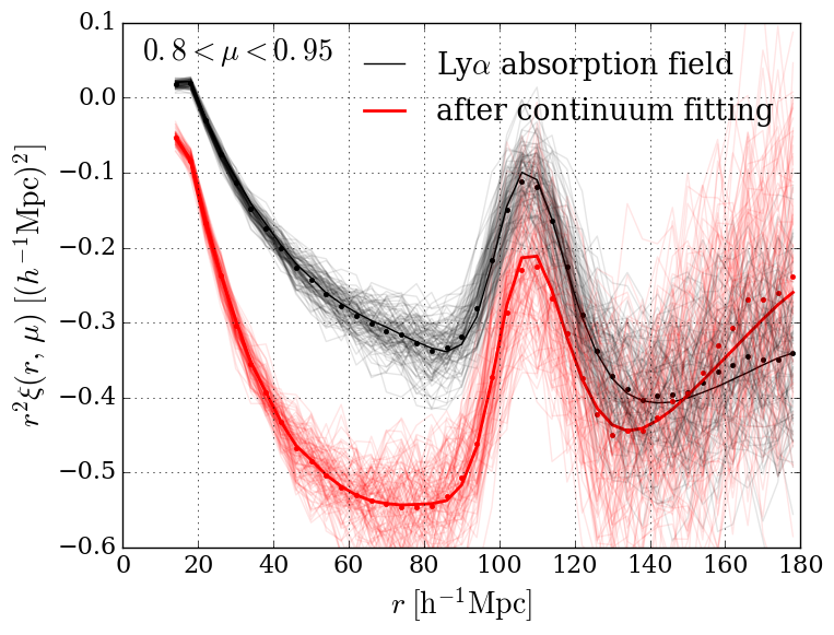
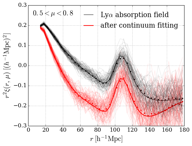
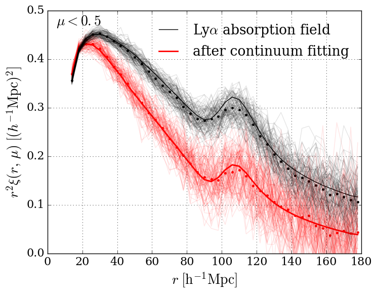
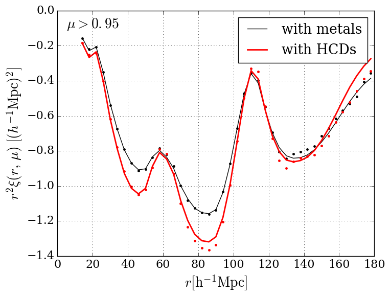
Four types of mocks were produced and analyzed. The results are summarized in table LABEL:fitmocktable and Figs. 11 and 12. The four types and the analysis procedure are as follows:

1. Only Ly$\alpha$ absorption: in the fits the distortion matrix is set to the identity matrix and only the parameters $(\alpha_{\perp},\alpha_{\parallel},b_{\rm Ly\alpha},\beta_{\rm Ly\alpha})$ are fit.

2. A quasar continuum is added: the fits use the distortion matrix and the parameters $(\alpha_{\perp},\alpha_{\parallel},b_{\rm Ly\alpha},\beta_{\rm Ly\alpha})$ are fit.

3. Metal absorption is added: the additional parameters are the $(b_{i},\beta_{i})$ for each metal transition, $i$.

4. High column density systems are added: three additional parameters $(b_{\rm HCD},\beta_{\rm HCD},L_{\rm HCD})$ are fit.

Figure 14: Measured correlation function in four ranges of $\mu$. The most radial range (top-left $\mu>0.95$) has, in addition to the BAO peak at $\sim 100\leavevmode\nobreak\ h^{-1}{\rm Mpc}$, a peak at $\sim 60\leavevmode\nobreak\ h^{-1}{\rm Mpc}$ due to correlated absorption by Ly$\alpha$ and SiIII(119.0,119.3) at the same physical position. In the next radial bin (top-right, $0.8<\mu<0.95$) only the BAO peak is visible. The lines show fits including successively Ly$\alpha$ and metal absorption, unidentified HCDs absorption, UV flux fluctuations, and a $(i_{\rm min},i_{\rm max},j_{\rm max})=(0,2,6)$ broadband (BB).

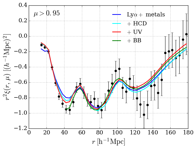
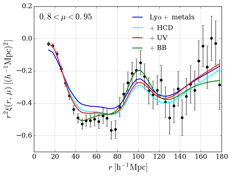
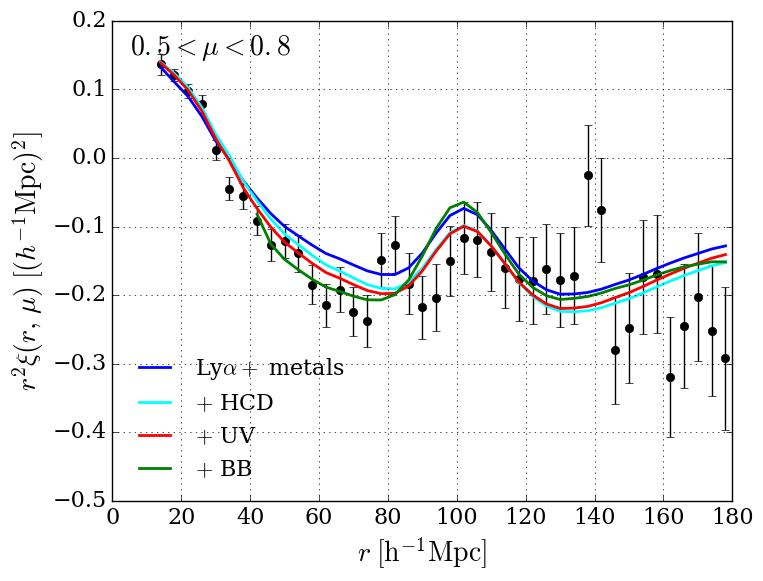
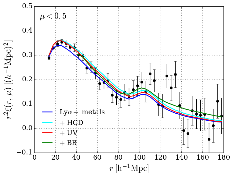
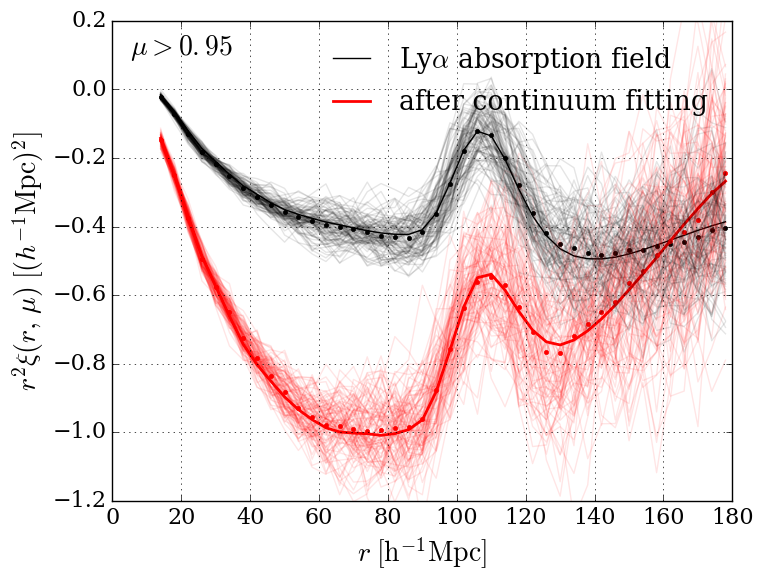
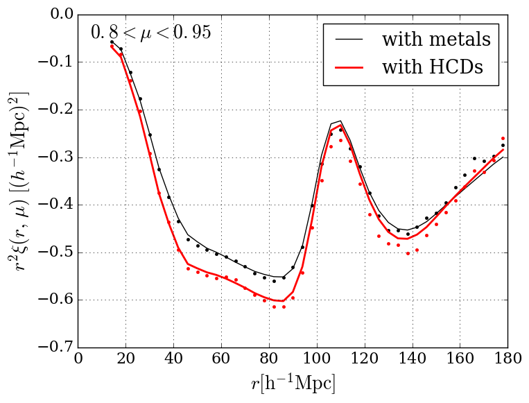
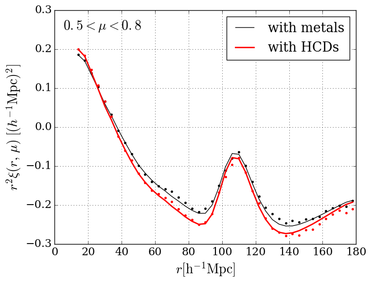
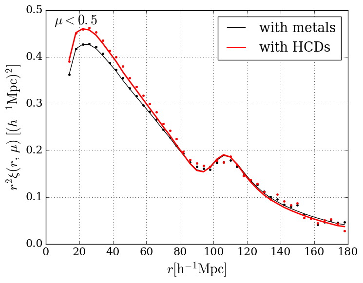
Figure 11 shows the correlation function in four ranges of $\mu$. The black points are the stack of the measured correlation function for type 1 mocks (only Ly$\alpha$ absorption). The red points are the stacked measurements for type 2 mocks (quasar continuum added). The difference between the black and red points shows the effect of continuum-fitting. The heavy curves are the best fit model for the cosmology used to generate the mocks. The good agreement between the red curve and points indicates the accuracy of the modeling of the continuum-fitting distortion.

Fits with type 3 mocks (including metals) were used to search for possible influences of metal absorption on derived BAO parameters. Metal absorption is mostly confined to the small $r_{\perp}$ region and this is seen in the two top panels of Fig. 12. The most radial sector, $\mu>0.95$, displays the effects of metal absorption, most prominently the peak due to SiIIa,b absorption around $r\sim 60\leavevmode\nobreak\ h^{-1}{\rm Mpc}$. The peak is not visible in the next sector, $0.8<\mu<0.95$.

Two sets of fits for type 4 mocks (HCDs) were also performed. In one, HCDs with $N_{\rm HI}<10^{20}{\rm cm^{-2}}$ were not given the DLA treatment described in Section 4.1. This cut approximates the threshold for DLA detection either automatically or visually. In the second set, only HCDs with $N_{\rm HI}>10^{21}\leavevmode\nobreak\ {\rm cm^{-2}}$ were treated specially, testing our sensitivity to an underestimation of the efficiency to flag DLAs.

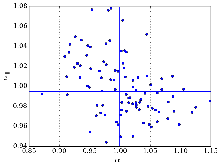
Table LABEL:fitmocktable lists the mean fit values for the 100 mocks and for the 4 types. Fig. 13 presents the corresponding distributions for type 4 mocks. For all types, the mean of the best-fit values of $(\alpha_{\perp},\alpha_{\parallel})$ is consistent with unity at the sub-percent level. Since the precision of our measurement with the data is of order three percent, this means that the mocks do not indicate any significant bias in the measurement of the BAO peak position.

6.3 Fits of the data with physical correlation function

Table 5: Results of fits of the data assuming increasingly complicated forms for $\xi^{\rm ph}(r_{\perp},r_{\parallel})$: Ly$\alpha$ absorption only; including metal absorption; including unidentified HCDs; and including fluctuations in the ionizing UV flux (i.e. the complete physical model whose complete set of parameters is given in Table 3). Fits are over the range $10<r<180\leavevmode\nobreak\ h^{-1}{\rm Mpc}$. The bias parameter, $b_{\rm Ly\alpha}$, refers to the reference redshift $z=2.3$.

analysis	$\alpha_{\parallel}$	$\alpha_{\perp}$	$b_{\rm Ly\alpha}(1+\beta_{\rm Ly\alpha})$	$\beta_{\rm Ly\alpha}$	$\chi^{2}_{\rm min}/DOF$, prob
Ly$\alpha$	$1.040\pm 0.033$	$0.975\pm 0.056$	$-0.326\pm 0.002$	$1.246\pm 0.044$	$1763.8/(1590-4)\;\;p=0.001$
+metals	$1.050\pm 0.035$	$0.967\pm 0.054$	$-0.330\pm 0.002$	$1.275\pm 0.045$	$1644.5/(1590-9)\;\;p=0.130$
+HCD	$1.053\pm 0.036$	$0.962\pm 0.054$	$-0.321\pm 0.003$	$1.656\pm 0.086$	$1561.4/(1590-12)\;\;p=0.612$
+UV	$1.053\pm 0.036$	$0.965\pm 0.055$	$-0.326\pm 0.003$	$1.666\pm 0.085$	$1556.5/(1590-13)\;\;p=0.639$

Table 6: Best-fit values of $(\alpha_{\perp},\alpha_{\parallel})$ for fits including metals, HCDs and UV fluctuations, with and without power-law broadbands (BBs) of the form $(i_{\rm min},i_{\rm max},j_{\rm max})=(0,2,6)$. The fit without broadbands is over $10<r<180\leavevmode\nobreak\ h^{-1}{\rm Mpc}$ and those with broadbands are over $40<r<180\leavevmode\nobreak\ h^{-1}{\rm Mpc}$. The broadband fit with “physical priors” requires that the best-fit values for parameters be within two standard deviations of those found without the broadband and imposes $A_{\rm peak}=1$. The broadband fit with “no additional priors” adds no constraints beyond fixing the parameters that are fixed in the fit without broadband (see Table 3).

analysis	$\alpha_{\parallel}$	$\alpha_{\perp}$	$\alpha_{\parallel}^{0.7}\alpha_{\perp}^{0.3}$	$\chi^{2}_{\rm min}/DOF$, prob.
no BB	$1.053^{+0.037\;+0.077}_{-0.035\;-0.071}$	$0.965^{+0.061\;+0.146}_{-0.051\;-0.102}$	$1.026^{+0.025\;+0.052}_{-0.024\;-0.047}$	$1556.5/(1590-13)\;0.639$
BB, physical priors	$1.057^{+0.039\;+0.081}_{-0.037\;-0.073}$	$0.962^{+0.063\;+0.155}_{-0.053\;-0.106}$	$1.028^{+0.026\;+0.054}_{-0.025\;-0.049}$	$1475.8/(1515-25)\;0.598$
BB, no additional priors	$1.043^{+0.035\;+0.075}_{-0.033\;-0.068}$	$1.000^{+0.095\;+0.346}_{-0.060\;-0.114}$	$1.030^{+0.023\;+0.063}_{-0.021\;-0.043}$	$1472.6/(1515-26)\;0.614$

The data were fit over the range $10<r<180\leavevmode\nobreak\ h^{-1}{\rm Mpc}$ under various hypotheses of increasing complexity concerning the form of $\xi^{\rm ph}(r_{\perp},r_{\parallel})$. The results are summarized in Table LABEL:fitautotable. The first fit assumes only Ly$\alpha$ absorption, the second includes absorption by metals, and the third absorption by unidentified HCDs. The fourth fit also assumes fluctuation in the flux of ionizing UV radiation. Inclusion of each effect yields a significantly better $\chi^{2}$; however, the values of $(\alpha_{\perp},\alpha_{\parallel})$ do not change significantly with each step. The data and fit correlation functions are presented for the four angular ranges in Fig. 14.

In what follows, we will focus our attention on the fourth fit that will be referred to as the “complete physical model”. The BAO peak-position parameters for this model are

$$\alpha_{\parallel}=1.053\pm 0.036\hskip 14.22636pt\Rightarrow\frac{D_{H}(z=2.33)}{r_{d}}=9.07\pm 0.31$$ (27)

$$\alpha_{\perp}=0.965\pm 0.055\hskip 14.22636pt\Rightarrow\frac{D_{M}(z=2.33)}{r_{d}}=37.77\pm 2.13\;.$$ (28)

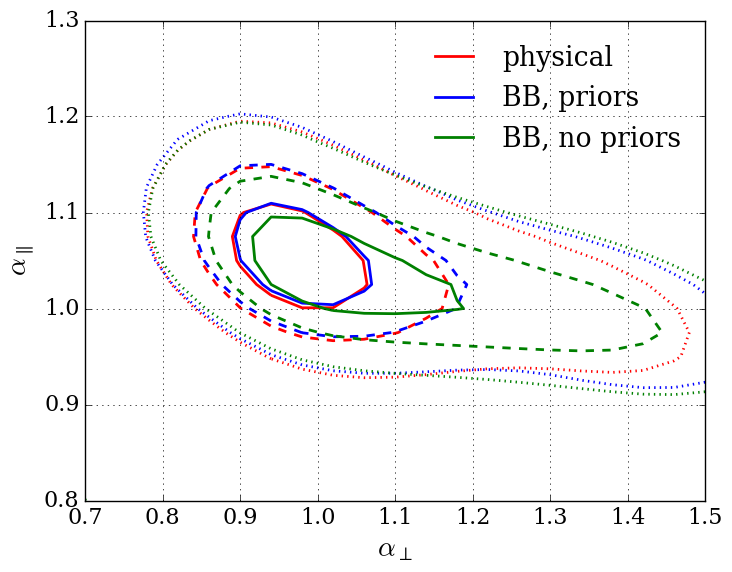
where we have used the Planck values from Table 1 that were used in the (angle,redshift) to $(r_{\perp},r_{\parallel})$ transformation. The one, two and three standard deviation contours (corresponding to $\Delta\chi^{2}=2.3,6.18,11.83$) are shown as the red contours in Fig. 15. Our result is within one standard deviation of the prediction of flat-$\Lambda$CDM model of Table 1 that is in agreement with the Planck data.

In the next Section we will study the robustness of the determination of the BAO-peak position parameters by adding power-law broadband terms to the complete physical model. We can also estimate the significance of the BAO peak by modifying this model by setting $A_{\rm peak}=0$. This degrades the quality of the fit by $\Delta\chi^{2}=27.7$ corresponding to a BAO peak detection of $5.2\sigma$. Adding broadband terms reduces this to $\Delta\chi^{2}=21.8$ ($4.7\sigma$).

Other than $(\alpha_{\perp},\alpha_{\parallel})$, the parameters of the model listed in Table 3 have no direct cosmological implications. However, the fact that the best-fit values are physically reasonable reinforces our confidence in the model and, therefore, on the cosmological conclusions. Most importantly, the best-fit values of $(b_{\rm Ly\alpha},\beta_{\rm Ly\alpha})$ in table LABEL:fitautotable are both relatively stable and near the expected values. For example, the model of Arinyo-i-Prats et al. (2015) predicts $\beta_{\rm Ly\alpha}\sim 1.4$ and $|b_{\rm Ly\alpha}|(1+\beta_{\rm Ly\alpha})$ in the range 0.25 to 0.33. In Appendix B we discuss in more detail the comparison of our measurement of $(b_{\rm Ly\alpha},\beta_{\rm Ly\alpha})$ with theory and with previous measurements.

The best-fit values of most of the other parameters in Table 3 are near those found in the mock fits. For the metal biases, this only means that we have placed a reasonable amount of metal absorption in the mock spectra. Of more significance is the value of $L_{\rm HCD}=(24.3\pm 1.13)\leavevmode\nobreak\ h^{-1}{\rm Mpc}$ which is, as expected, roughly the width of a DLA of $N_{\rm HI}=10^{20}\leavevmode\nobreak\ {\rm cm^{2}}$, corresponding to our estimated threshold for good efficiency in identifying DLAs. In the mocks, best-fit values of $L_{\rm HCD}$ when masking only those DLAs with $N_{\rm HI}>10^{20}\leavevmode\nobreak\ {\rm cm^{2}}$ cluster near $L_{\rm HCD}\sim 25$ in about half the fits. For the other half, the fits find $L_{\rm HCD}\sim 0$, corresponding to the addition of a second Ly$\alpha$ component but with a different $\beta$. This indicates that more than one way exists to model sufficiently well the correlation function with unidentified HCDs. The bias parameter found in the data, $b_{\rm HCD}=-0.0288\pm 0.0043$, is about a factor of 7 higher than that found in those mocks that find $L_{\rm HCD}\sim 25$. This indicates that there are unidentified HCDs in the data with $N_{\rm HI}>10^{20}{\rm cm^{2}}$ and or that the HCDs that we have placed in the mocks are less biased than in reality.

We have not generated mocks with fluctuations in the flux of ionizing radiation. However, we note that the bias parameter $b_{\Gamma}=0.1125\pm 0.0511$ is near the value of $0.13$ suggested by Gontcho A Gontcho et al. (2014).

6.4 Fits of the data with power-law broadbands added

In addition to statistical uncertainties, it is important to determine to what extent the derived values of $(\alpha_{\perp},\alpha_{\parallel})$ are influenced by the assumed form of $\xi^{\rm ph}$. The amplitude and form of the metal components are well understood and constrained by the low-$r_{\perp}$ bins. However, the HCD and UV parameters have a more diffuse effect on the correlation function and are not strongly constrained by independent data. For example, the UV background fluctuation model we have used includes only fluctuations that follow the underlying density field. Additional correlations (Gontcho A Gontcho et al., 2014) due to the discrete nature of sources of UV radiation would modify the absorption in neighboring forests since they are influenced by the same discrete sources. This “shot-noise” term would give an additive, isotropic and positive contribution to the Ly$\alpha$ auto-correlation function. Its shape and amplitude as a function of comoving separation are however poorly known as they depend on the quasar luminosity distribution and variability.

To study the effects of possible uncertainties in the form of the non-BAO component, $\xi^{\rm ph}_{\rm smooth}$, we have performed fits adding to the complete physical model broadband functions in the form of power laws (26) defined by $(i_{\rm min},i_{\rm max},j_{\rm max})$. With the addition of new components of $\xi^{\rm ph}_{\rm smooth}$, the connection between the BAO peak amplitude and the smooth components is lost so we also performed fits releasing the constraint $A_{\rm peak}=1$.

The parameters of slowly varying broadband forms are necessarily somewhat degenerate with the parameters of the slowly varying part of the physical model: $(b,\beta)$ and the parameters describing HCDs and UV fluctuations. As such, fits with power-law broadband terms can produce unphysical best-fit values of these parameters. Conversely, we expect that a small number of power-law terms will not significantly affect the BAO-peak parameters. Fits with the mock spectra indicate that this is the case if the power-law broadbands are restricted to the ranges $-2\leq i_{\rm max}\leq 3$, $(i_{\rm max}-i_{\rm min})\leq 3$ and $j_{\rm max}\leq 6$. Of course in the case of the mocks we know precisely the form of the physical correlation function while for the data we do not. Shifts of ($\alpha_{\perp},\alpha_{\parallel}$) in the data when using power-law terms could indicate that the underlying physical correlation function has not been modeled with sufficient precision.

We want to ensure that the power-law terms model variations of the slowly-varying part of the correlation function under the BAO peak. We therefore perform these fits only over the restricted range $40<r<180\leavevmode\nobreak\ h^{-1}{\rm Mpc}$, avoiding undue influence of the $10<r<40\leavevmode\nobreak\ h^{-1}{\rm Mpc}$ range on the amplitudes of the power laws. Using this range, the fit with the complete physical model without power-law broadbands yields BAO parameters indistinguishable from those found over the full range $10<r<180\leavevmode\nobreak\ h^{-1}{\rm Mpc}$ (Table LABEL:fitautotable).

To choose appropriate values of $(i_{\rm min},i_{\rm max},j_{\rm max})$, we note that apart from the BAO peak, $r^{2}\xi$ does not vary wildly over the range $40<r<180\leavevmode\nobreak\ h^{-1}{\rm Mpc}$. A reasonable choice is therefore $(i_{\rm min},i_{\rm max})=(0,2)$ corresponding to a parabola and which amounts to freeing the value and first two derivatives of $r^{2}\xi_{\rm smooth}$ underneath the BAO peak. A reasonable choice for $j_{\rm max}$ is $j_{\rm max}=6$ corresponding to approximately independent broadbands in each of the four angular ranges in Fig. 14. The best-fit correlation function for $(i_{\rm min},i_{\rm max},j_{\rm max})=(0,2,6)$ and $A_{\rm peak}$ free is shown in the figure and the BAO-peak parameters on the third line of Table LABEL:fitbroadbandtable. The best-fit value of $\alpha_{\parallel}$ is $\sim 1\%$ (i.e. $\sim 0.3\sigma$) lower than the value for the complete physical model and uncertainty is unchanged. The value of $\alpha_{\perp}$ is about 3% higher than the standard value with the error increasing slightly from $\sim 0.055$ to $\sim 0.075$. The one- and two-standard deviation contours are shown in green in Fig. 15. We emphasize that these results are obtained without placing any priors on the physical parameters, other than those already used in the standard fits.

We have experimented with other combinations of $(i_{\rm min},i_{\rm max},j_{\rm max})$ in the range $j_{\rm max}\leq 6$, $-2<i_{\rm min}<0$, $-1<i_{\rm max}<3$. While most combinations yield values of $(\alpha_{\perp},\alpha_{\parallel})$ that are close to the nominal values, there are cases where there are significant changes. These cases always correspond to fits yielding unphysical values for $(b,\beta)$ of one or more components. In all cases, the large changes in $(\alpha_{\perp},\alpha_{\parallel})$ can be avoided by placing a “physical priors” on the $(b,\beta)$ that requires them to take values within two standard deviations of those found in the standard fits over the range $10<r<180\leavevmode\nobreak\ h^{-1}{\rm Mpc}$ and imposing $A_{\rm peak}=1$. The results for the $(0,2,6)$ model are listed oneline two of Table LABEL:fitbroadbandtable and the contours shown in blue in Fig. 15.

Figure 15: Contours for $(\alpha_{\perp},\alpha_{\parallel})$ at the (68.3, 95.45, 99.73)% CL (solid, dashed, dotted). The red contours are for the physical model with HCDs and UV fluctuations from Tables 3 and LABEL:fitautotable. The blue (green) contours are for the $(i_{\rm min},i_{\rm max},j_{\rm max})=(0,2,6)$ power-law broadband with (without) priors on the parameters of the physical correlation function.

6.5 Summary of data fits

Table LABEL:fitbroadbandtable and Fig. 15 summarizes the BAO parameters found for fits with our most complete physical model of the correlation function, with and without power-law broadbands. The results of the fits with physical priors imply that the uncertainty in the form of $\xi^{\rm ph}_{\rm smooth}$ does not translate into a significant uncertainty in $(\alpha_{\perp},\alpha_{\parallel})$. Because of the priors placed on the physical parameters, this conclusion follows only if our basic physical model is not too far removed from reality. Without such priors, the uncertainty of $\alpha_{\perp}$ can be significantly increased (line 3 of Table LABEL:fitbroadbandtable).

The limits on $\alpha_{\parallel}$ are relatively stable with the inclusion of broadbands. A quantity that is more robust than either $\alpha_{\parallel}$ or $\alpha_{\perp}$ is $\alpha_{\parallel}^{\gamma}\alpha_{\perp}^{1-\gamma}$ with the exponent $\gamma$ chosen to minimize the variance. For the observed correlation and variances of $(\alpha_{\perp},\alpha_{\parallel})$, one calculates $\gamma\sim 0.7$ with

$$\alpha_{\parallel}^{0.7}\alpha_{\perp}^{0.3}=1.028\pm 0.026\;,$$ (29)

where the uncertainty is chosen to cover the one-standard-deviations of the three fits in Table LABEL:fitbroadbandtable. Using the Planck model values from Table 1, we deduce

$$\frac{D_{H}^{0.7}D_{M}^{0.3}}{r_{d}}=13.94\pm 0.35\hskip 14.22636pt{\rm at}\;z=2.33\;.$$ (30)

This result is largely independent of the addition of power-law broadbands. It contains most of the cosmological constraints of our measurement if used in combination with constraints from the forest-quasar cross-correlation, since the latter has more constraining power on $D_{M}/r_{d}$ than the auto-correlation result.

6.6 Comparison with previous results

We can compare the results (27) and (28) with those of Delubac et al. (2015): $D_{H}(2.34)/r_{d}=9.18\pm 0.28$, $D_{M}/r_{d}=37.67\pm 2.17$ and $D_{H}^{0.7}D_{M}^{0.3}/r_{d}=14.02\pm 0.3$. The change in $D_{H}/r_{d}$ is $\sim 0.5\sigma$. To determine whether this change is due to the change in analysis procedure or in the data set we performed fits using only data used in the DR11 analysis. The results for a HCDS,UV analysis are $D_{H}(2.33)/r_{d}=9.14\pm 0.28$ and $D_{M}(2.34)/r_{d}=37.54\pm 2.17$, within $0.15\sigma$ and $0.06\sigma$ of the results of Delubac et al. (2015). This result implies that most of the change is due to the change in the data set.

The $0.5\sigma$ change in $D_{H}/r_{d}$ is typical of the variations we can expect when increasing the sample size from DR11 to DR12. We confirmed this expectations by using jackknife samples of DR12 to simulate DR11 data sets and observing changes in $D_{H}/r_{d}$. Roughly 30% of the jackknife samples had a change as large as that observed for DR11 and we therefore conclude that the DR12-DR11 difference is primarily statistical.

Table 7: Systematic shifts of the Ly$\alpha$ bias parameters and BAO peak-position parameters due to various spurious correlations discussed in Sect. 5. Individual shifts in $(\alpha_{\perp},\alpha_{\parallel})$ are less than $\sigma/10$ and the total shifts are consistent with zero. Their uncertainty is dominated by the statistical uncertainty on the sky model.

	$\beta_{\rm Ly\alpha}$	$b(1+\beta)$	$\alpha_{\parallel}$	$\alpha_{\perp}$
Sky model noise	$-0.026$	$-0.002$	$<0.001$	$<0.001$
Calibration noise	$+0.047$	$+0.002$	$<0.001$	$+0.001$
Fiber cross-talk	$+0.003$	$<0.001$	$<0.001$	$<0.001$
ISM absorption	$+0.003$	$<0.001$	$<0.001$	$<0.001$
Sum	$+0.027$	$<0.001$	$+0.001$	$<0.001$
Quadratic sum	$+0.054$	$+0.002$	$<0.001$	$+0.001$

Figure 16: Derivative of the normalized Ly$\alpha$-forest flux-decrement, $\delta_{LyaF}$, with respect to the Milky Way dust column density normalized to its dispersion. The dashed curves represent the 0,1,2 and 3-$\sigma$ uncertainties. The red vertical lines mark the positions of the calcium H and K lines.

7 Systematic Errors in the BAO-peak position

Systematic errors in $(\alpha_{\perp},\alpha_{\parallel})$ can result if the measured correlations function is not sufficiently well modeled by the fitting function (18). Such effects can be introduced by the pipeline and analysis procedures, by improper modeling for the flux-transmission field, and by astrophysical absorption not related to cosmological large-scale structure.

Spurious correlations introduced by the pipeline were discussed in Section 5. The most important correlations were confined to the lowest $r_{\parallel}$ bin with negligible effects on the fitting of the correlation function. No evidence was found for any additional instrumental correlations that could have an influence of the measurement of $(\alpha_{\perp},\alpha_{\parallel})$. Since our model of pipeline-induced correlations introduces no scales near the BAO scale, it is not surprising that it predicts negligible effects on the BAO scale. Upper limits on the pipeline-induced shifts in $(\alpha_{\perp},\alpha_{\parallel})$ are given in Table 7.

Biases could also be introduced at the analysis level, for example through the small correlations between weights and the measured $\delta_{q}(\lambda)$. These correlations are estimated to have a negligible impact on the BAO parameters. If they did not, they would have produced biased estimates of $(\alpha_{\perp},\alpha_{\parallel})$ in the mock data sets, while no such biases are seen.

The second type of systematic error would result from incorrect modeling of the various contributions to the physical correlations. The physical correlations are parameterized by the $(b_{i},\beta_{i})$ for each transition. These parameters are marginalized over and their uncertainties therefore contribute to the reported statistical errors on $(\alpha_{\perp},\alpha_{\parallel})$.

Modeling of the contribution of unidentified HCDs and of UV fluctuations also contain free-parameters that are marginalized over. We have verified that the best-fit BAO parameters are insensitive to assumption about non-linearities and redshift evolution of the bias parameters. We have also investigated possible influence of foreground absorbers in addition to CIV. Finally, we have included power-law broadband parameters to place limits on our sensitivity to unmodeled slowly-varying contributions.

In our physical model of the correlation function we have ignored two effects that could potentially bias our results at some level. First, we have assumed that the lines of sight sample random positions of the Universe, while in a real survey we only have information in pixels in front of a quasar. This makes our measured correlation sensitive to the three-point function of quasar-lya-lya, but given that this is averaged over pixel pairs at different separations from the quasars we expect this contamination to be very smooth on BAO scales. The second effect is that the transmitted flux fraction could be affected by the relative velocity between baryons and dark matter in the early Universe (Tseliakhovich & Hirata, 2010). These relative velocities are quite small in the redshift range of interest, but it is possible that the different velocities at early times left an imprint in the distribution of neutral hydrogen even at low redshift, similar to what has been suggested in the case of galaxy clustering (Dalal et al., 2010; Yoo et al., 2011; Blazek et al., 2016). In order to study this effect in the Lyman alpha forest we would require detailed hydrodynamical simulations, and this is beyond the scope of this paper. Given that the density of quasars should have a different dependency on the relative velocity, differences in the BAO scale measured from the auto-correlation and from the cross-correlation with quasars (Font-Ribera et al., 2014) could be used to constraint the amplitude of this effect.

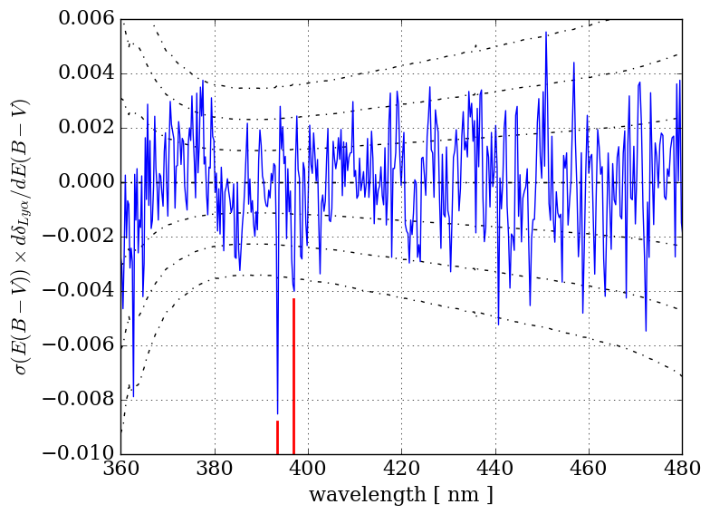
The third type of systematic error would be due to correlations of non-cosmological origin. One possibility is atomic or molecular absorption in the Galactic interstellar medium (ISM). The average ISM absorption is included in the fit mean flux transmission, or the subsequent subtraction of the average $\delta_{q}(\lambda)$. However, residuals correlated across the sky might still be present. Current studies show that the ISM absorption is highly correlated with dust column density. We hence use the estimated Milky-Way dust extinction as a proxy for potential ISM absorption and fit for the correlation of $\delta_{q}(\lambda)$ with this dust extinction parameter. The resulting correlation is shown in Fig. 16. The Ca H and K lines are the only known ISM lines to appear significantly. Therefore ISM absorption has a negligible impact on the Ly$\alpha$ correlation function. We have verified this conclusion by computing the auto-correlation function of the quantity $E(B-V)\times d\delta_{q}(\lambda)/dE(B-V)$.

A final source of correlations that we have considered would originate in our use of a unique quasar-continuum template which we adapt to individual quasars by the $(a_{q},b_{q})$ parameters of equation 3. Templates could be improved by making them depend on a non-forest variable, like quasar redshift or CIV emission-line strength. These improved templates could change the derived flux correlation function if the non-forest variables of the quasars are themselves correlated at large distances. This is not expected to be the case of CIV line strength since this strength is believed to be due to local conditions and therefore not correlated at large distances. We have tested this by using two templates, one for strong CIV emitters (relative to side-bands) and one for weak emitters. This slightly improves the pixel variance (by 3%) but makes no significant change in the measured correlation function and less than $0.1\%$ difference in the derived $(\alpha_{\perp},\alpha_{\parallel})$.

Figure 17: Comoving expansion rate, $r_{d}H(z)/(1+z)$, measured with BAO, with $r_{d}$ in units of 147.3 Mpc. The red square is the present measurement at $z=2.33$. Also shown are measurements using the Ly$\alpha$-quasar cross correlation at $z=2.36$ (Font-Ribera et al., 2014), and galaxy correlations at $0.35<z<0.65$ (Alam et al., 2016), at $z=0.15$ (Ross et al., 2015), and at $z=0.11$ (Beutler et al., 2011). The points at $z=0.11$ and $z=0.15$ use the SNIa measurement of $q_{0}$ (Betoule et al., 2014) to convert the measured $D_{V}(z)\propto D_{M}^{2/3}D_{H}^{1/3}$ to $D_{H}(z)$. The black line is the prediction of the Planck flat $\Lambda$CDM model (table 1).

Figure 18: One- and two-standard deviation constraints on the o$\Lambda$CDM parameters $(\Omega_{M},\Omega_{\Lambda})$ using BAO measurements of $D_{M}(z)/r_{d}$ and $D_{H}(z)/r_{d}$ without CMB measurements, i.e. without imposing the CMB value of $r_{d}$. The red contours use the work presented here (line 1 of Table LABEL:fitbroadbandtable), the $z<0.8$ galaxy data (Alam et al., 2016; Beutler et al., 2011; Ross et al., 2015) and the quasar-forest cross-correlation (Font-Ribera et al., 2014). The gray contours exclude the quasar-forest cross-correlation. The blue contours use only the $z<0.8$ galaxy data and the green contours show the constraints derived from the SNIa Hubble diagram (Betoule et al., 2014). The black dot is the position of the flat-$\Lambda$CDM model that describes CMB data (Planck Collaboration et al., 2016).

A continuum that evolves with redshift could be more problematic because the correlation function measurement necessarily requires quasar pairs that are near in redshift. We searched for the effect of such evolution by using a quasar continuum template that evolves linearly in redshift. The results do not differ significantly from those for the redshift-independent template.

We have searched for unsuspected systematics by dividing the data into two redshift bins, $z<2.295$ and $z>2.295$. The 95%CL ranges on $\alpha_{\parallel}$ in the high and low redshift ranges are $0.90<\alpha_{\parallel}<1.094$ and $1.02<\alpha_{\parallel}<1.15$. For $\alpha_{\perp}$ the ranges are $0.74<\alpha_{\perp}<1.5$ and $0.86<\alpha_{\perp}<1.01$. As with the DR11 results of Delubac et al. (2015), the results are consistent with the expected absence of evolution at the two-standard-deviation level.

8 Cosmological implications

Our measurements of $D_{M}/r_{d}$ and $D_{H}/r_{d}$ at $z=2.33$ are in good agreement with the values predicted by the flat-$\Lambda$CDM model consistent with the CMB data. The precision is, however, less than that of the BOSS galaxy BAO data (Alam et al., 2016), and for simple cosmological models, parameter constraints based on combinations of CMB and BAO data are not strongly changed by our results. Our constraints however, can provide tests of more general models with complicated expansion dynamics (Aubourg et al., 2015).

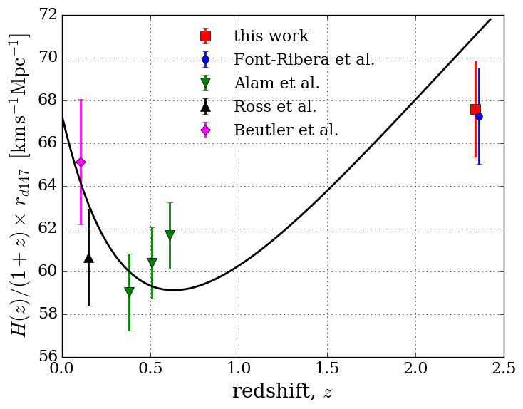
When combined with other BAO data, our measurement provides interesting results using only low-redshift data. For example, the low-redshift expansion history can be directly measured through the measurements of $D_{H}(z)/r_{d}$. The Hubble distance (27) can be written as

$$H(z=2.33)=(224.\pm 8.)\leavevmode\nobreak\ {\rm km\,s^{-1}Mpc^{-1}}\frac{147.33\leavevmode\nobreak\ {\rm Mpc}}{r_{d}}$$ (31)

Figure 17 displays this result along with those of Alam et al. (2016); Beutler et al. (2011); Ross et al. (2015) and Font-Ribera et al. (2014). The expected phases of acceleration at $z<0.7$ and deceleration at $z>0.7$ are striking.

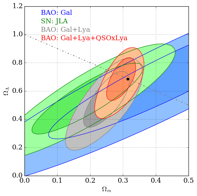
Combining $D_{H}/r_{d}$ and $D_{M}/r_{d}$ measurements, the cosmological parameters can be measured independently of CMB data. Non-flat $\Lambda$CDM models (o$\Lambda$CDM ) have three parameters $(\Omega_{M},\Omega_{\Lambda},H_{0}r_{d})$ that determine $D_{M}/r_{d}$ and $D_{H}/r_{d}$ and constraints on $(\Omega_{M},\Omega_{\Lambda})$ can be derived by marginalizing over $H_{0}r_{d}$. This procedure is equivalent to the use of SNIa to measure $(\Omega_{M},\Omega_{\Lambda})$ by marginalizing over the parameters that determine supernova luminosities. Fig. 18 shows the constraints derived using various combinations of BAO results. By themselves, the low-redshift BAO data provide no strong evidence for $\Omega_{\Lambda}>0$. The inclusion of the Ly$\alpha$-forest data results in $\sim 10\%$ precision on $(\Omega_{M},\Omega_{\Lambda})$:

$$\Omega_{M}=0.296\pm 0.029\hskip 28.45274pt\Omega_{\Lambda}=0.699\pm 0.100$$ (32)

consistent with spatial flatness:

$$\Omega_{k}=-0.002\pm 0.119\;.$$ (33)

The fit has $\chi^{2}=12.27$ for 12 data points and three parameters. The values of $(\Omega_{M},\Omega_{\Lambda})$ agree well with the flat-$\Lambda$CDM values found using CMB anisotropies $(\Omega_{M},\Omega_{\Lambda})=(0.315,0.685)$ (Planck Collaboration et al., 2016).

9 Conclusions

In this paper, we present an analysis of the complete SDSS-3 (DR12) set of Ly$\alpha$ forests. The position of the BAO peak in the flux correlation function is in good agreement with that expected in flat-$\Lambda$CDM models favored by CMB anisotropies.

Our analysis represents a significant improvement over our previous work, both in the understanding of instrumental effects on the flux transmission and in the data analysis. The modeling of the distortion of the correlation function due to continuum fitting allows fitting the entire correlation function using a physical model without resorting to arbitrary “broadband terms”. In the future, this approach may allow alternative ways to study the cosmological parameters, for instance by eliminating the need to separate the correlation function into “smooth” and “peak” components.

Now that we have direct access to the full correlation function, further improvements in the analysis will profit from better modeling of absorption mechanisms. In particular, it will be important to fully use external constraints on HCD and metal absorption.

The improvements in modeling and data analysis that we have implemented here will clearly be important for future projects with reduced statistical errors. For example, the DESI project (DESI Collaboration et al., 2016) will have up to 15 times the number of forest-pixel pairs resulting in a significant decrease of statistical errors of the correlation function. The understanding the physics of the broadband correlation function may be the limiting factor in the extraction of BAO parameters.

The cosmological information from the Ly$\alpha$-forest auto-correlation function studied here is complemented by the study of the cross-correlation between the forest and neighboring quasars. Results and implications of a new measurement of this function will be presented in a forthcoming publication (du Mas des Bourboux et al., in preparation).

Appendix A Modifications applied to the BOSS spectral extraction pipeline

Each of the two BOSS spectrograph slitheads consists of 500 fibers organized in 25 aligned blocks (or bundles) of 20 fibers (see Smee et al. 2013 for a description of the BOSS spectrographs). Fibers in a bundle are separated by 260 $\mu$m whereas the separation between fibers of adjacent bundles is 624 $\mu$m. This design allows one to treat independently each fiber bundle in the data reduction: whereas the overlap of light coming from fibers of the same bundle must be accounted for, one can safely ignore interbundle contamination.

The spectral processing consists in a row-by-row extraction from each CCD, where the signal of a row of pixels illuminated by a fiber bundle is fit independently from the rest of the data (wavelength are dispersed approximately along CCD columns). The extraction consists in minimizing the following quantity

$$\chi^{2}=\sum_{pixel\ i}w_{i}\left(D_{i}-\sum_{fiber\ f}\hat{N}_{f}\,\hat{P}_{f,i}-\sum_{k}a_{k}i^{k}\right)^{2}$$

where $D$ are the pixel values (after preprocessing, i.e. after the subtraction of the bias, conversion from digital units to electrons, and flat-fielding), $w$ the weights assigned to each pixel, $P$ the true cross-dispersion PSF profile of a fiber and $\hat{P}$ the profile used (a Gaussian). The quantity $\hat{N}$ is the number of collected electrons from a fiber, to be estimated. The last term is a low-order polynomial contribution used to fit any residual light in the row; it compensates both for scattered light and the imperfect modeling of the cross-dispersion profile tails.

For the extraction to be optimal, one must have $w_{i}=var_{i}^{-1}$, where $var_{i}$ is the variance of $D_{i}$. This pixel variance is, however, not known a priori. In the BOSS DR12 pipeline, the pixel data were directly used as an estimate of the expected signal: $var_{i}=var_{read}+D_{i}$ if $D_{i}>0$ and $var=var_{read}$ if not, where $var_{read}$ is the readout noise variance, and $D_{i}$ is here an estimate of the Poisson noise.

This use of the data to determine the variance results in a biased estimate of the flux. As an illustration, if one considers a single fiber extraction, without the background polynomial contribution, the $\chi^{2}$ minimization yields

$$\hat{N}=\frac{\sum_{i}w_{i}D_{i}\hat{P}_{i}}{\sum_{i}w_{i}\hat{P}_{i}^{2}}$$

To first order, assuming $D_{i}=NP_{i}+\delta_{i}>0$, and noting $\bar{w}_{i}=1/var(\delta_{i})$ the expectation value of $w_{i}$, one has $w_{i}\simeq\bar{w}_{i}(1-\bar{w}_{i}\delta_{i})$ and

$$\hat{N}\simeq N\frac{\sum_{i}\bar{w}_{i}P_{i}\hat{P}_{i}}{\sum_{i}\bar{w}_{i}\hat{P}_{i}^{2}}-\frac{\sum_{i}\bar{w}_{i}\hat{P}_{i}}{\sum_{i}\bar{w}_{i}\hat{P}_{i}^{2}}$$ (34)

The first term produces an unbiased estimate of $N$ if $\hat{P}=P$, which is not strictly the case. This bias is in principle corrected for by the calibration, but since the weights $\bar{w}$ depend on the amount of signal, the calibration obtained with bright spectra does not perfectly correct the bias of faint spectra. The second term is a systematic underestimation of the signal; it can be interpreted as an effective number of pixels contributing to the measurement (if the profile is normalized, with $\sum_{i}P_{i}=1$).

The fractional bias is more important at low fluxes, and as a consequence i) this bias has a non trivial wavelength dependence correlated with bright sky emission lines and ii) its amplitude relative to the calibrated flux depends on the throughput and hence the observation conditions. Those two effects could lead to correlated biases in the Ly$\alpha$ forest.

We have rerun the data processing using $w_{i}=1/var_{read}$ (this weight is in practice not a constant quantity per CCD amplifier because of the flat-field correction). We also improved the outlier rejection procedure that discards unmasked pixels affected by cosmic rays.

This new approach to extraction is unbiased but less optimal. Expressing this procedure using a matrix representation, if we define $X$ as the parameters of the model (fluxes and polynomial corrections) such that we can interpret the data as $D=HX+\delta$ (where $\delta$ is the noise), the optimal extraction results in a covariance of the parameters $C_{X}=(\sum_{i}w_{i}H_{i}H_{i}^{T})^{-1}$, whereas the sub-optimal extraction produces a larger covariance $C_{X}^{\prime}=C_{X}(\sum w_{i}^{2}var_{i}H_{i}H_{i}^{T})C_{X}$. We use this latter expression in the subsequent steps of the pipeline, using the estimated flux (and not directly the pixel values) to evaluate the Poisson noise contribution to $var_{i}$.

The ratio of uncertainties does not exceed 5% over the dynamic range of BOSS observations of quasars. It reaches a higher value of 10% for the brightest measurements (see Fig. 19).

Subsequent steps of the data processing (fiber flat-field, sky spectrum model, photometric calibration) also involve the weighted average of the data. Similarly to the extraction, using directly the flux inverse variances as weights results in a bias because of the flux-inverse-variance correlation. We hence took care of replacing the inverse variances of spectra by their average over many wavelength (using a spline fit) to mitigate this bias and to simultaneously minimize the loss of optimality. Those changes have been incorporated in the pipeline used for the SDSS data release DR13 (SDSS Collaboration et al., 2016).

Figure 19: Comparison of flux measurement uncertainties between the DR12 data reduction (in blue) and this new extraction (in red). This analysis is based on the data from camera b1, plate 7339, where many observations of the same targets were performed. The top panel shows the empirical r.m.s. (circles) among the various observations, and the corresponding predicted uncertainty (lines) of the number of electrons per CCD row ($N_{e}$) as a function of $N_{e}$. The second panel is the same quantity normalized by the predicted uncertainty of DR12. The bottom panel displays the fraction of 3 $\sigma$ outliers that were discarded in the two other panels. As expected, there is a larger dispersion with the new, less optimal reduction at high flux. The larger dispersion at low flux is not easy to understand; it is probably a consequence of the biased estimator in DR12, where negative statistical fluctuations are given a high weight.

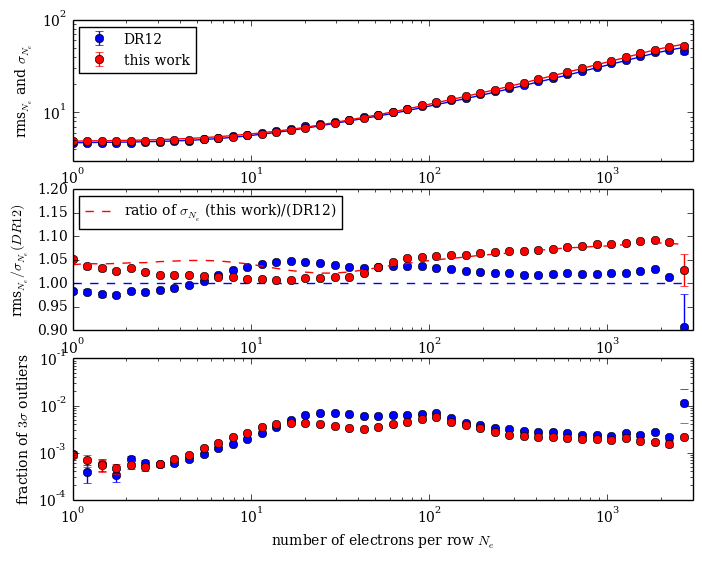
Appendix B The bias parameters of the Ly$\alpha$ forest

The physical model of the Ly$\alpha$ forest autocorrelation function involves two independent parameters for the linear biasing: the density bias factor $b_{\rm Ly\alpha}$, and the redshift distortion factor $\beta_{\rm Ly\alpha}$. The values for our best fit with errors are given in Table 5. As usual, we give the value of $b_{\rm Ly\alpha}(1+\beta_{\rm Ly\alpha})$ because its error is smaller than the error for $b_{\rm Ly\alpha}$ and less correlated with $\beta_{\rm Ly\alpha}$ (see Slosar et al. (2011)). Some variations of these parameters occur as the model is improved to include the effects of metal lines, and possible effects of HCDs and ionizing intensity fluctuations. As expected, there is a degeneracy in the values of various parameters of the model that affect broadband terms. In particular, the value of $\beta_{\rm Ly\alpha}$ shows a substantial change from 1.2 to 1.7 depending on the model that is used. The first model, assuming that only Ly$\alpha$ forest correlation is present with a constant ionizing intensity, does not yield a good fit. Taking into account the effect of metal lines is the main improvement of the model that allows for an acceptable fit, and does not change appreciably the value of $\beta_{\rm Ly\alpha}$ although errors are substantially increased. The addition of the effects of HCDs and UV fluctuations further improves the model and increases substantially the best fit value of $\beta_{\rm Ly\alpha}$.

To compare our values of $b$ and $\beta_{\rm Ly\alpha}$ with the previous determination from the DR11 data from Blomqvist et al. (2015), we first translate their result to the cosmological model we use in this paper, taking into account that the measurement of the Ly$\alpha$ autocorrelation depends only on $b\sigma_{8}(\bar{z})$, where $\bar{z}=2.33$ is the mean redshift of our Ly$\alpha$ forest correlation measurement. Blomqvist et al. (2015) measured $\beta_{\rm Ly\alpha}=1.39\pm 0.11$, and $b_{\rm Ly\alpha}(1+\beta_{\rm Ly\alpha})=-0.374\pm 0.007$, using a model with $\Omega_{m}=0.27$ and $\sigma_{8}=0.7877$, implying $\sigma_{8}(\bar{z})=0.3072$. The model used in this paper has $\Omega_{m}=0.3147$ and $\sigma_{8}=0.8298$, implying $\sigma_{8}(\bar{z})=0.3131$. Therefore the Ly$\alpha$ bias of Blomqvist et al. (2015) translated to our model is $b_{\rm Ly\alpha}(1+\beta_{\rm Ly\alpha})=-0.367\pm 0.007$. This should be compared with our result on the first row of Table 5, because Blomqvist et al. (2015) did not consider the effects from metals, HCDs or UV fluctuations

The main reason for the difference with the values of $b_{\rm Ly\alpha}(1+\beta_{\rm Ly\alpha})$ and $\beta_{\rm Ly\alpha}$ we obtain here for our Ly$\alpha$ forest model applied to DR12 given in Table 5 is the different radial range for the fit: Blomqvist et al. (2015) restricted their fit to $r>40\leavevmode\nobreak\ h^{-1}{\rm Mpc}$, whereas we use $r>10\leavevmode\nobreak\ h^{-1}{\rm Mpc}$. There are other details that contribute to the difference, e.g., the continuum distortion and bin smoothing modeling, but the radial range of the fit is most important. As mentioned earlier, the $\chi^{2}$ value shows that our Ly$\alpha$ fit is not good, reflecting the fact that the shape of the correlation cannot be properly fit over our broad radial range. This is why the values of $\|b_{\rm Ly\alpha}\|\,(1+\beta_{\rm Ly\alpha})$ and $\beta_{\rm Ly\alpha}$ decrease when extending the fit to smaller separations. The better fits obtained for the more complete models in Table 5 show that $b_{\rm Ly\alpha}(1+\beta_{\rm Ly\alpha})$ is relatively stable, but the value of $\beta_{\rm Ly\alpha}$ can be more model dependent.

These results can also be compared to theoretical predictions from hydrodynamic simulations of the intergalactic medium, which were compared to the observational measurement of Blomqvist et al. (2015) in Section 7 of Arinyo-i-Prats et al. (2015). There, it was noticed that while the predicted value of $\beta_{\rm Ly\alpha}$ is roughly in agreement with the observational determination, the value of $\|b_{\rm Ly\alpha}\|\,(1+\beta_{\rm Ly\alpha})$ was predicted to be lower than observed. Now, the lower value of $\|b_{\rm Ly\alpha}\|\,(1+\beta_{\rm Ly\alpha})$ we measure from DR12, correcting for the effect of metals and extending the fit to smaller separations, is in much better agreement with the range of the expected theoretical values. Despite the considerable uncertainties that are still present both in the predictions from hydrodynamic simulations of the Ly$\alpha$ forest (as discussed in Arinyo-i-Prats et al. (2015)), and in the observational determinations that are affected by the modeling of metals, HCDs and ionizing intensity fluctuations, we think that the rough agreement we now find of two independently predicted linear bias factors of the Ly$\alpha$ forest is fairly remarkable. In the future, we expect to be able to better measure these linear factors and their redshift evolution.

References

- Alam et al. (2015) Alam, S., Albareti, F. D., Allende Prieto, C., et al. 2015, ApJS, 219, 12
- Alam et al. (2016) Alam, S., Ata, M., Bailey, S., et al. 2016, ArXiv e-prints [arXiv:1607.03155]
- Anderson et al. (2014a) Anderson, L., Aubourg, É., Bailey, S., et al. 2014a, MNRAS, 441, 24
- Anderson et al. (2014b) Anderson, L., Aubourg, E., Bailey, S., et al. 2014b, MNRAS, 439, 83
- Anderson et al. (2012) Anderson, L., Aubourg, E., Bailey, S., et al. 2012, MNRAS, 427, 3435
- Arinyo-i-Prats et al. (2015) Arinyo-i-Prats, A., Miralda-Escudé, J., Viel, M., & Cen, R. 2015, J. Cosmology Astropart. Phys., 12, 017
- Aubourg et al. (2015) Aubourg, É., Bailey, S., Bautista, J. E., et al. 2015, Phys. Rev. D, 92, 123516
- Bautista et al. (2015) Bautista, J. E., Bailey, S., Font-Ribera, A., et al. 2015, J. Cosmology Astropart. Phys., 5, 60
- Becker et al. (1995) Becker, R. H., White, R. L., & Helfand, D. J. 1995, ApJ, 450, 559
- Betoule et al. (2014) Betoule, M., Kessler, R., Guy, J., et al. 2014, A&A, 568, A22
- Beutler et al. (2011) Beutler, F., Blake, C., Colless, M., et al. 2011, MNRAS, 416, 3017
- Blake et al. (2011) Blake, C., Davis, T., Poole, G. B., et al. 2011, MNRAS, 415, 2892
- Blazek et al. (2016) Blazek, J. A., McEwen, J. E., & Hirata, C. M. 2016, Physical Review Letters, 116, 121303
- Blomqvist et al. (2015) Blomqvist, M., Kirkby, D., Bautista, J. E., et al. 2015, J. Cosmology Astropart. Phys., 11, 034
- Bolton et al. (2012) Bolton, A. S., Schlegel, D. J., Aubourg, É., et al. 2012, AJ, 144, 144
- Bovy et al. (2011) Bovy, J., Hennawi, J. F., Hogg, D. W., et al. 2011, ApJ, 729, 141
- Busca et al. (2013) Busca, N. G., Delubac, T., Rich, J., et al. 2013, A&A, 552, A96
- Chuang & Wang (2012) Chuang, C.-H. & Wang, Y. 2012, MNRAS, 426, 226
- Cole et al. (2005) Cole, S., Percival, W. J., Peacock, J. A., et al. 2005, MNRAS, 362, 505
- Croft et al. (2016) Croft, R. A. C., Miralda-Escudé, J., Zheng, Z., et al. 2016, MNRAS, 457, 3541
- Croom et al. (2005) Croom, S. M., Boyle, B. J., Shanks, T., et al. 2005, MNRAS, 356, 415
- Dalal et al. (2010) Dalal, N., Pen, U.-L., & Seljak, U. 2010, J. Cosmology Astropart. Phys., 11, 007
- Dawson et al. (2013) Dawson, K. S., Schlegel, D. J., Ahn, C. P., et al. 2013, AJ, 145, 10
- Delubac et al. (2015) Delubac, T., Bautista, J. E., Busca, N. G., et al. 2015, A&A, 574, A59
- DESI Collaboration et al. (2016) DESI Collaboration, Aghamousa, A., Aguilar, J., et al. 2016, ArXiv e-prints [arXiv:1611.00036]
- Eisenstein et al. (2011) Eisenstein, D. J., Weinberg, D. H., Agol, E., et al. 2011, AJ, 142, 72
- Eisenstein et al. (2005) Eisenstein, D. J., Zehavi, I., Hogg, D. W., et al. 2005, ApJ, 633, 560
- Font-Ribera et al. (2013) Font-Ribera, A., Arnau, E., Miralda-Escudé, J., et al. 2013, J. Cosmology Astropart. Phys., 5, 18
- Font-Ribera et al. (2014) Font-Ribera, A., Kirkby, D., Busca, N., et al. 2014, J. Cosmology Astropart. Phys., 5, 27
- Font-Ribera et al. (2012) Font-Ribera, A., McDonald, P., & Miralda-Escudé, J. 2012, J. Cosmology Astropart. Phys., 1, 1
- Font-Ribera & Miralda-Escudé (2012) Font-Ribera, A. & Miralda-Escudé, J. 2012, J. Cosmology Astropart. Phys., 7, 28
- Gontcho A Gontcho et al. (2014) Gontcho A Gontcho, S., Miralda-Escudé, J., & Busca, N. G. 2014, MNRAS, 442, 187
- Gunn et al. (1998) Gunn, J. E., Carr, M., Rockosi, C., et al. 1998, AJ, 116, 3040
- Gunn et al. (2006) Gunn, J. E., Siegmund, W. A., Mannery, E. J., et al. 2006, AJ, 131, 2332
- Kirkby et al. (2013) Kirkby, D., Margala, D., Slosar, A., et al. 2013, J. Cosmology Astropart. Phys., 3, 24
- Kirkpatrick et al. (2011) Kirkpatrick, J. A., Schlegel, D. J., Ross, N. P., et al. 2011, ApJ, 743, 125
- Lawrence et al. (2007) Lawrence, A., Warren, S. J., Almaini, O., et al. 2007, MNRAS, 379, 1599
- Lewis et al. (2000) Lewis, A., Challinor, A., & Lasenby, A. 2000, ApJ, 538, 473
- Margala et al. (2016) Margala, D., Kirkby, D., Dawson, K., et al. 2016, ApJ, 831, 157
- Martin et al. (2005) Martin, D. C., Fanson, J., Schiminovich, D., et al. 2005, ApJ, 619, L1
- McDonald (2003) McDonald, P. 2003, ApJ, 585, 34
- McDonald & Eisenstein (2007) McDonald, P. & Eisenstein, D. J. 2007, Phys. Rev. D, 76, 063009
- Mehta et al. (2012) Mehta, K. T., Cuesta, A. J., Xu, X., Eisenstein, D. J., & Padmanabhan, N. 2012, MNRAS, 427, 2168
- Noterdaeme et al. (2012) Noterdaeme, P., Petitjean, P., Carithers, W. C., et al. 2012, A&A, 547, L1
- Padmanabhan et al. (2012) Padmanabhan, N., Xu, X., Eisenstein, D. J., et al. 2012, MNRAS, 427, 2132
- Pâris et al. (2012) Pâris, I., Petitjean, P., Aubourg, É., et al. 2012, A&A, 548, A66
- Pâris et al. (2014) Pâris, I., Petitjean, P., Aubourg, É., et al. 2014, A&A, 563, A54
- Pâris et al. (2016) Pâris, I., Petitjean, P., Ross, N. P., et al. 2016, ArXiv e-prints [arXiv:1608.06483]
- Peebles & Yu (1970) Peebles, P. J. E. & Yu, J. T. 1970, ApJ, 162, 815
- Percival et al. (2007) Percival, W. J., Cole, S., Eisenstein, D. J., et al. 2007, MNRAS, 381, 1053
- Percival et al. (2010) Percival, W. J., Reid, B. A., Eisenstein, D. J., et al. 2010, MNRAS, 401, 2148
- Pieri et al. (2010) Pieri, M. M., Frank, S., Weinberg, D. H., Mathur, S., & York, D. G. 2010, ApJ, 724, L69
- Pieri et al. (2014) Pieri, M. M., Mortonson, M. J., Frank, S., et al. 2014, MNRAS, 441, 1718
- Planck Collaboration et al. (2014) Planck Collaboration, Ade, P. A. R., Aghanim, N., et al. 2014, A&A, 571, A16
- Planck Collaboration et al. (2016) Planck Collaboration, Ade, P. A. R., Aghanim, N., et al. 2016, A&A, 594, A13
- Pontzen (2014) Pontzen, A. 2014, Phys. Rev. D, 89, 083010
- Prochaska et al. (2005) Prochaska, J. X., Herbert-Fort, S., & Wolfe, A. M. 2005, ApJ, 635, 123
- Ross et al. (2015) Ross, A. J., Samushia, L., Howlett, C., et al. 2015, MNRAS, 449, 835
- Ross et al. (2012) Ross, N. P., Myers, A. D., Sheldon, E. S., et al. 2012, ApJS, 199, 3
- Rudie et al. (2013) Rudie, G. C., Steidel, C. C., Shapley, A. E., & Pettini, M. 2013, ApJ, 769, 146
- SDSS Collaboration et al. (2016) SDSS Collaboration, Albareti, F. D., Allende Prieto, C., et al. 2016, ArXiv e-prints [arXiv:1608.02013]
- Slosar et al. (2011) Slosar, A., Font-Ribera, A., Pieri, M. M., et al. 2011, J. Cosmology Astropart. Phys., 9, 1
- Slosar et al. (2013) Slosar, A., Iršič, V., Kirkby, D., et al. 2013, J. Cosmology Astropart. Phys., 4, 26
- Smee et al. (2013) Smee, S. A., Gunn, J. E., Uomoto, A., et al. 2013, AJ, 146, 32
- Sunyaev & Zeldovich (1970) Sunyaev, R. A. & Zeldovich, Y. B. 1970, Ap&SS, 7, 3
- Suzuki (2006) Suzuki, N. 2006, ApJS, 163, 110
- Suzuki et al. (2005) Suzuki, N., Tytler, D., Kirkman, D., O’Meara, J. M., & Lubin, D. 2005, ApJ, 618, 592
- Tseliakhovich & Hirata (2010) Tseliakhovich, D. & Hirata, C. 2010, Phys. Rev. D, 82, 083520
- Xu et al. (2013) Xu, X., Cuesta, A. J., Padmanabhan, N., Eisenstein, D. J., & McBride, C. K. 2013, MNRAS, 431, 2834
- Yèche et al. (2010) Yèche, C., Petitjean, P., Rich, J., et al. 2010, A&A, 523, A14
- Yoo et al. (2011) Yoo, J., Dalal, N., & Seljak, U. 2011, J. Cosmology Astropart. Phys., 7, 018