Dark matter statistics for large galaxy catalogs: power spectra and covariance matrices

Abstract

Upcoming and existing large-scale surveys of galaxies require accurate theoretical predictions of the dark matter clustering statistics for thousands of mock galaxy catalogs. We demonstrate that this goal can be achieve with our new Parallel Particle-Mesh (PM) $N$-body code (PPM-GLAM) at a very low computational cost. We run about 15,000 simulations with $\sim 2$ billion particles that provide $\sim 1$% accuracy of the dark matter power spectra $P(k)$ for wave-numbers up to $k\sim 1h{\rm Mpc}^{-1}$. Using this large data-set we study the power spectrum covariance matrix, the stepping stone for producing mock catalogs. In contrast to many previous analytical and numerical results, we find that the covariance matrix normalised to the power spectrum $C(k,k^{\prime})/P(k)P(k^{\prime})$ has a complex structure of non-diagonal components. It has an upturn at small $k$, followed by a minimum at $k\approx 0.1-0.2\,h{\rm Mpc}^{-1}$. It also has a maximum at $k\approx 0.5-0.6\,h{\rm Mpc}^{-1}$. The normalised covariance matrix strongly evolves with redshift: $C(k,k^{\prime})\propto\delta^{\alpha}(t)P(k)P(k^{\prime})$, where $\delta$ is the linear growth factor and $\alpha\approx 1-1.25$, which indicates that the covariance matrix depends on cosmological parameters. We also show that waves longer than $1\mbox{$h^{-1}$Gpc}$ have very little impact on the power spectrum and covariance matrix. This significantly reduces the computational costs and complexity of theoretical predictions: relatively small volume $\sim(1\mbox{$h^{-1}$Gpc})^{3}$ simulations capture the necessary properties of dark matter clustering statistics. All the power spectra obtained from many thousands of our simulations are publicly available.

1 Introduction

Accurate theoretical predictions for the clustering properties of different galaxy populations are crucial for the success of massive observational surveys such as SDSS-III/BOSS (e.g., Alam et al., 2016), SDSS-IV/eBOSS (Dawson et al., 2016), DESI (DESI Collaboration et al., 2016) and Euclid (Laureijs et al., 2011) that have or will be able to measure the positions of millions of galaxies. The predictions of the statistical properties of the distribution of galaxies expected in modern cosmological models involve a number of steps: it starts with the generation of the dark matter clustering and proceeds with placing “galaxies” according to some bias prescriptions (see Chuang et al., 2015; Monaco, 2016, for a review).

While a substantial effort has been made to estimate the non-linear matter power spectrum $P(k)$ (e.g., Smith et al., 2003; Heitmann et al., 2009; Schneider et al., 2016), the covariance matrix is a much less studied quantity that is required for the analysis of the observational data. Most of the time the main attention shifts to the last step, i.e., the placement of “galaxies” in the density field with all the defects and uncertainties of estimates of the dark matter distribution and velocities being often incorporated into the biasing scheme (e.g., Chuang et al., 2015). However, one needs to accurately reproduce and to demonstrate that whatever algorithm or prescription is adopted to mock galaxies, also is able to match the clustering and covariance matrix of the dark matter field.

The covariance matrix $C(k,k^{\prime})$ is the second-order statistics of the power spectrum: $C(k,k^{\prime})=\langle P(k)P(k^{\prime})\rangle-\langle P(k)\rangle\langle P(k^{\prime})\rangle$, where $\langle\dots\rangle$ implies averaging over an ensamble of realizations. The power spectrum covariance and its cousin the covariance of the correlation function play an important role in estimates of the accuracy of measured power spectrum, and the inverse covariance matrices are used in estimates of cosmological parameters deduced from these measurements (e.g., Anderson et al., 2012; Sánchez et al., 2012; Dodelson & Schneider, 2013; Percival et al., 2014). The power spectrum covariance matrix measures the degree of non-linearity and mode coupling of waves with different wave-numbers. As such it is an interesting entity on its own.

Because it is expensive to produce thousands of simulations (e.g., Taylor et al., 2013; Percival et al., 2014) using standard high-resolution $N$-body codes, there were relatively few publications on the structure and evolution of the covariance matrix. Most of the results are based on simulations with relatively small number of particles (16 million as compared with our $\sim 2$ billion) and small computational volumes of $500-600\,\mbox{$h^{-1}$Mpc}$ (Takahashi et al., 2009; Li et al., 2014; Blot et al., 2015). There was no systematic analysis of the effects of mass, force resolution and volume on the covariance matrix.

So far, there are some uncertainties and disagreements even on the shape of the covariance matrix. Neyrinck (2011); Mohammed & Seljak (2014); Carron et al. (2015) argue that once the Gaussian diagonal terms are removed, the covariance function should be a constant. This disagrees with numerical (Li et al., 2014; Blot et al., 2015) and analytical (Bertolini et al., 2016; Mohammed et al., 2016) results that indicate that the non-diagonal components of the covariance matrix have quite complex structure.

There are also issues and questions related with numerical simulations. How many realizations are needed for accurate measurements of the covariance matrix (Taylor et al., 2013; Percival et al., 2014) and how can it be reduced (Pope & Szapudi, 2008; Pearson & Samushia, 2016; Joachimi, 2017)? What resolution and how many time-steps are needed for accurate estimates? How large the simulation volume should be to adequately probe relevant scales and to avoid defects related with the box size (Gnedin et al., 2011; Li et al., 2014)?

The goal of our paper is to systematically study the structure of the matter covariance matrix using a large set of $N$-body simulations. The development of $N$-body cosmological algorithms has been an active field of research for decades. However, the requirements for the generation of many thousands of high-quality simulations are extreme. Existing codes such as GADGET, RAMSES, or ART are powerful for large high-resolution simulations, but they are not fast enough for medium quality large-number of realisations required for analysis and interpretation of large galaxy surveys. New types of codes (e.g., White et al., 2014; Tassev et al., 2013; Feng et al., 2016) are being developed for this purpose. Here, we present the performance results of our new $N$-body Parallel Particle-Mesh GLAM code (PPM-GLAM), which is the core of the GLAM (GaLAxy Mocks) pipeline for the massive production of large galaxy catalogs. PPM-GLAM generates the density field, including peculiar velocities, for a particular cosmological model and initial conditions.

The optimal box size of the simulations is of particular interest for producing thousands of mock galaxy catalogs and for the studies of large-scale galaxy clustering. With the upcoming observational samples tending to cover larger observational volumes ($\sim 50\,{\rm Gpc}^{3}$), one naively expects that the computational volumes should be large enough to cover the entire observational sample. Indeed, this will be the ideal case, if we were to measure some statistics that involve waves as long as the whole sample. The problem with producing extra large simulations is their computational cost. For accurate predictions one needs to maintain the resolution on small scales. With a fixed resolution the cost of computations scales with volume. So, it increases very quickly and becomes prohibitively expensive.

However, most of the observable clustering statistics rely on relatively small scales, and thus would not require extra large simulation boxes. For example, the Baryonic Acoustic Oscillations (BAO) are on scales of $\sim 100\,\mbox{$h^{-1}$Mpc}$ and the power spectrum of galaxy clustering is typically measured on wave-numbers $k\mbox{${\,\hbox{\hbox{$>$}\kern-8.00003pt\lower 4.30554pt\hbox{$\sim$}}\,}$}0.05\,h{\rm Mpc}^{-1}$. In order to make accurate theoretical predictions for these scales, we need relatively small $\sim 1\,\mbox{$h^{-1}$Gpc}$ simulation volumes.

What will be the consequences of using small computational volumes? One may think about few. For example, long-waves missed in small simulation boxes may couple with small-scale waves and produce larger power spectrum (and potentially covariance matrix). This is the so called Super Sample Covariance (SSC, Gnedin et al., 2011; Li et al., 2014; Wagner et al., 2015; Baldauf et al., 2016). Another effect is the statistics of waves. By replicating and stacking small boxes (to cover large observational volumes) we do not add the statistics of small waves, which we are interested in. For example, the number of pairs with separation of say $100\,\mbox{$h^{-1}$Mpc}$ will be defined only by how many independent pairs are in a small box, and not by the much larger number of pairs found in large observational samples. These concerns are valid, but can be resolved in a number of ways. SSC effects depend on the volume and become very small as the computational volume increases. Statistics of waves can be re-scaled proportionally to the volume (e.g., Mohammed & Seljak, 2014; Bertolini et al., 2016). We investigate these issues in detail in our paper, together with the performance of the power spectrum depending on the numerical parameters of our PPM-GLAM simulations. All the power spectra obtained from many thousands of our simulations are made publicly available.

In Section 2 we discuss the main features of our PPM-GLAM simulation code. More detailed description and tests are presented in the Appendixes. The suite of simulations used in this paper is presented in Section 3. Convergence and accuracy of the power spectrum are discussed in Section 4. The results on the covariance matrix of the power spectrum are given in Section 5. We campare our results with other works in Section 6. Summary and discussion of our results are presented in Section 7.

Table 1: Numerical and cosmological parameters of different simulations. The columns give the simulation identifier, the size of the simulated box in $h^{-1}\,{\rm Mpc}$, the number of particles, the mass per simulation particle $m_{p}$ in units $h^{-1}\,M_{\odot}$, the mesh size $\mbox{$N_{\rm g}$}^{3}$, the gravitational softening length $\epsilon$ in units of $h^{-1}\,{\rm Mpc}$, the number of time-steps $N_{s}$, the amplitude of perturbations $\sigma_{8}$, the matter density $\Omega_{m}$, the number of realisations $N_{r}$ and the total volume in $[h^{-1}\,{\rm Gpc}]^{3}$

Simulation	Box	particles	$m_{p}$	$\mbox{$N_{\rm g}$}^{3}$	$\epsilon$	$N_{\rm s}$	$\sigma_{8}$	$\Omega_{m}$	$N_{r}$	Total Volume
PPM-GLAM A0.5	5003	12003	$6.16\times 10^{9}$	24003	0.208	181	0.822	0.307	680	85
PPM-GLAM A0.9	9603	12003	$4.46\times 10^{10}$	24003	0.400	136	0.822	0.307	2532	2240
PPM-GLAM A1.5	15003	12003	$1.66\times 10^{11}$	24003	0.625	136	0.822	0.307	4513	15230
PPM-GLAM A2.5	25003	10003	$1.33\times 10^{12}$	20003	1.250	136	0.822	0.307	1960	30620
PPM-GLAM A4.0	40003	10003	$5.45\times 10^{12}$	20003	1.250	136	0.822	0.307	4575	292800
PPM-GLAM B1.0a	10003	16003	$2.08\times 10^{10}$	32003	0.312	147	0.828	0.307	10	10
PPM-GLAM B1.0b	10003	13003	$1.78\times 10^{10}$	26003	0.385	131	0.828	0.307	10	10
PPM-GLAM B1.5	15003	13003	$3.88\times 10^{10}$	26003	0.577	131	0.828	0.307	10	33
PPM-GLAM C1a	10003	10003	$8.71\times 10^{10}$	30003	0.333	302	0.828	0.307	1	1
PPM-GLAM C1b	10003	10003	$8.71\times 10^{10}$	40003	0.250	136	0.828	0.307	1	1
BigMDPL1	25003	38403	$2.4\times 10^{10}$	–	0.010	–	0.828	0.307	1	15.6
HMDPL1	40003	40963	$7.9\times 10^{10}$	–	0.025	–	0.828	0.307	1	64
Takahashi et al.2	10003	2563	$1.8\times 10^{12}$	–	–	–	0.760	0.238	5000	5000
Li et al.3	5003	2563	$2.7\times 10^{11}$	–	–	–	0.820	0.286	3584	448
Blot et al.4	6563	2563	$1.2\times 10^{12}$	–	–	–	0.801	0.257	12288	3469
BOSS QPM5	25603	12803	$3.0\times 10^{11}$	12803	2.00	7	0.800	0.29	1000	16700
WiggleZ COLA6	6003	12963	$7.5\times 10^{9}$	$3888^{3}$	–	10	0.812	0.273	3600	778
References: 1Klypin et al. (2016), 2Takahashi et al. (2009), 3Li et al. (2014), 4Blot et al. (2015),
References: 5White et al. (2014), 6Koda et al. (2016)

2 Parallel Particle-Mesh GLAM code

There are a number of advantages of cosmological Particle-Mesh (PM) codes (Klypin & Shandarin, 1983; Hockney & Eastwood, 1988; Klypin & Holtzman, 1997) that make them useful on their own to generating a large number of galaxy mocks (e.g., QPM, COLA, FastPM; White et al., 2014; Tassev et al., 2013; Feng et al., 2016), or as a component of more complex hybrid TREE-PM (e.g., Gadget2, HACC; Springel, 2005; Habib et al., 2014) and Adaptive-Mesh-Refinement codes (e.g. ART, RAMSES, ENZO; Kravtsov et al., 1997; Teyssier, 2002; Bryan et al., 2014). Cosmological PM codes are the fastest codes available and they are simple.

We have developed and thoroughly tested a new parallel version of the Particle-Mesh cosmological code, that provides us with a tool to quickly generate a large number of $N$-body cosmological simulations with a reasonable speed and acceptable resolution. We call our code Parallel Particle-Mesh GLAM (PPM-GLAM), which is the core of the GLAM (GaLAxy Mocks) pipeline for massive production of galaxy catalogs. PPM-GLAM generates the density field, including peculiar velocities, for a particular cosmological model and initial conditions. Appendix A gives the details of the code and provides tests for the effects of mass and force resolutions, and the effects of time-stepping. Here, we discuss the main features of the PPM-GLAM code and provide the motivation for the selection of appropriate numerical parameters.

The code uses a regularly spaced three-dimensional mesh of size $N_{\rm g}^{3}$ that covers the cubic domain $L^{3}$ of a simulation box. The size of a cell $\Delta x=L/N_{\rm g}$ and the mass of each particle $m_{\rm p}$ define the force and mass resolution respectively:

$$m_{\rm p} = \Omega_{m}\,\rho_{\rm cr,0}\left[\frac{L}{N_{\rm p}}\right]^{3}=$$ (1)

$$= 8.517\times 10^{10}\left[\frac{\Omega_{m}}{0.30}\right]\left[\frac{L/\mbox{$h^{-1}$Gpc}}{N_{\rm p}/1000}\right]^{3}h^{-1}M_{\odot},$$ (2)

$$\Delta x = \left[\frac{L/\mbox{$h^{-1}$Gpc}}{N_{\rm g}/1000}\right]\mbox{$h^{-1}$Mpc},$$ (3)

where $N_{\rm p}^{3}$ is the number of particles and $\rho_{\rm cr,0}$ is the critical density of the universe at present.

PPM-GLAM solves the Poisson equation for the gravitational potential in a periodical cube using a Fast Fourier Transformation (FFT) algorithm. The dark matter density field used in the Poisson equation is obtained with the Cloud-In-Cell (CIC) scheme using the positions of dark matter particles. Once the gravitational potential is obtained, it is numerically differentiated and interpolated to the position of each particle. Then, particle positions and velocities are advanced in time using the second order leap-frog scheme. The time-step is increased periodically as discussed in Appendix A. Thus, a standard PM code has three steps that are repeated many times until the system reached its final moment of evolution: (1) Obtain the density field on a 3D-mesh that covers the computational volume, (2) Solve the Poisson equation, and (3) Advance particles to the next moment of time.

The computational cost of a single PPM-GLAM simulation depends on the number of time-steps $N_{s}$, the size of the 3D-mesh $N_{\rm g}^{3}$, and the adopted number of particles $N_{\rm p}^{3}$. The CPU required to solve the Poisson equation is mostly determined by the cost of performing a single 1D-FFT. We incorporate all numerical factors into one coefficient and write the CPU for the Poisson solver as $AN_{\rm g}^{3}$. The costs of density assignment and particle displacement (including potential differentiation) scale proportionally to $N_{\rm p}^{3}$. In total, the CPU time $T_{\rm tot}$ required for a single PPM-GLAM run is:

$$T_{\rm tot}=\mbox{$N_{\rm s}$}\left[A\mbox{$N_{\rm g}$}^{3}+(B+C)\mbox{$N_{\rm p}$}^{3}\right],$$ (4)

where $B$ and $C$ are the coefficients for scaling the CPU estimate for particle displacements and density assignment. These numerical factors were estimated for different processors currently used for $N$-body simulations and are given in Table 3. For a typical simulation analysed in this paper ($\mbox{$N_{\rm g}$}=2400$, $\mbox{$N_{\rm p}$}=\mbox{$N_{\rm g}$}/2$) the CPU per time-step is $\sim 0.5$ hours and wall-clock time per step $\sim 1-3$ minutes. The total cost of 1000 PPM-GLAM realizations with $\mbox{$N_{\rm s}$}=150$ is 75K CPU hours, which is a modest allocation even for a small computational cluster or a supercomputer center.

Memory is another critical factor that should be considered when selecting the parameters of our simulations. PPM-GLAM uses only one 3D-mesh for storing both density and gravitational potential, and only one set of particle coordinates and velocities. Thus, for single precision variables the total required memory $M_{\rm tot}$ is:

$$M_{\rm tot} = 4N_{\rm g}^{3}+24N_{\rm p}^{3}\,\,{\rm Bytes},$$ (5)

$$= 29.8\left(\frac{\mbox{$N_{\rm g}$}}{2000}\right)^{3}+22.3\left(\frac{\mbox{$N_{\rm p}$}}{1000}\right)^{3}{\rm GB},$$ (6)

$$= 52\left(\frac{\mbox{$N_{\rm p}$}}{1000}\right)^{3}{\rm GB},\,\,{\rm for}\quad\mbox{$N_{\rm g}$}=2\mbox{$N_{\rm p}$}.$$ (7)

Figure 1: Power spectra of dark matter at redshift zero. The linear power spectrum is shown as a dotted line. Left: The PPM-GLAM simulations used for the plot are A0.5 (red full curve), A1.5 (black dot-dashed) and A2.5 (blue dashed). They closely reproduce the clustering of the high-resolution MultiDark simulations (black full curve) up to $k\approx 1\,h{\rm Mpc}^{-1}$ with exact deviations on larger $k$ depending on the force resolution. Right: Zoom-in on the region of the BAO peaks. The power spectra were multiplied by $k^{5/4}$ and arbitrarily normalised to reveal more clearly the differences between the simulations. Because there are only two realisations of the MultiDark simulations (BigMDPL & HMDPL), statistical deviations due to cosmic variance are seen at different $k$ (e.g., $k\approx 0.045,0.07\,h{\rm Mpc}^{-1}$). Cosmic variance of the simulations (errors of the mean) are nearly negligible because there are thousands of PPM-GLAM realisations. The deviations seen for the A0.5 points (red circles) at small $k$ are due to the large bin width, in $k$-space, for this simulation.

The number of time-steps $N_{\rm s}$ is proportional to the computational costs of the simulations. This is why reducing the number of steps is important for producing a large set of realisations. White et al. (2014) and Koda et al. (2016) use just $\sim 10$ time-steps for their QPM and COLA simulations. Feng et al. (2016) and Izard et al. (2015) advocate using $\mbox{$N_{\rm s}$}\approx 40$ steps for Fast-PM and ICE-COLA. The question still remains: what optimal number of time-steps should be adopted? However, there is no answer to this question without specifying the required force resolution, and without specifying how the simulations will be used to generate mock galaxies.

In Appendix B we provide a detailed discussion on the effects of time-stepping. We argue that for the stability and accuracy of the integration of the dark matter particle trajectories inside dense (quasi-) virialised objects, such as clusters of galaxies, the time-step $\Delta t$ must be smaller enough to satisfy the constraints given by eqs. (39) and (41). For example, FastPM simulations with 40 time-steps and force resolution of $\Delta x=0.2\,\mbox{$h^{-1}$Mpc}$ (see Feng et al., 2016) do not satisfy these conditions and would require 2-2.5 times more time-steps. However, a small number of time-steps manifests itself not in the power spectrum (though, some decline in $P(k)$ happens at $k\sim 1\,\mbox{$h^{-1}$Mpc}$). Its effect is mostly observed in a significantly reduced fraction of volume with large overdensities and random velocities, which potentially introduces undesirable scale-dependent bias.

Because our main goal is to produce simulations with the minimum corrections to the local density and peculiar velocities, we use $\mbox{$N_{\rm s}$}\approx 100-200$ time-steps in our PPM-GLAM simulations. This number of steps also removes the need to split particle displacements into quasi-linear ones and the deviations from quasi-linear predictions. Thus, in this way we greatly reduce the complexity of the code and increase its speed, while also substantially reduce the memory requirements.

3 Simulations

We made a large number of PPM-GLAM simulations – about 15,000 – to study different aspects of the clustering statistics of the dark matter density field in the flat $\Lambda$CDM Planck cosmology. The numerical parameters of our simulations are presented in Table 1. All the simulations were started at initial redshift $z_{\rm init}=100$ using the Zeldovich approximation. The simulations span three orders of magnitude in mass resolution, a factor of six in force resolution and differ by a factor of 500 in effective volume. To our knowledge this is the largest set of simulations available today. Power spectra and covariance matrices are publicly available in our Skies and Universes site.

The PPM-GLAM simulations labeled with letter A are the main simulations used for estimates of the power spectrum and the covariance matrix. Series B and C are designed to study different numerical effects. In particular, C1a are actually four simulations run with the different number of steps: $\mbox{$N_{\rm s}$}=34,68,147,302$. There are also four C1b simulations that differ by the force resolution: $\mbox{$N_{\rm g}$}=1000,2000,3000,4000$.

We compare the performance of our PPM-GLAM simulations with the results obtained from some of the MultiDark simulations run with L-Gadget2: BigMDPL and HMDMPL (see for details Klypin et al., 2016). The parameters of these large-box and high-resolution simulations are also presented in Table 1. For comparison we also list very large number of low resolution simulations performed by Takahashi et al. (2009), Li et al. (2014) and Blot et al. (2015) with the Gadget2, L-Gadget2 and AMR codes, respectively, to study the power spectrum covariances. Details of the QPM (White et al., 2014) and COLA (Koda et al., 2016) simulations that were used to generate a large number of galaxy mocks for the BOSS and WiggleZ galaxy redshift surveys are also given in Table 1. Note that the QPM simulations have very low force resolution, which requires substantial modeling on how dark matter should be clustered and moving on the scale of galaxies.

We estimate the power spectrum $P(k)$ of the dark matter density field in all our 10 simulation snapshots for each realisation, but in this paper we mostly focus on the $z=0$ results. For each simulation we estimate the density on a 3D-mesh of the size indicated in Table 1. We then apply FFT to generate the amplitudes of the Fourier harmonics $\delta_{i,j,k}$ in phase-space. The spacing of the Fourier harmonics is equal to the length of the fundamental harmonic $\Delta\kappa\equiv 2\pi/L$. Thus, the wave-vector ${\bf k}_{i,j,k}$ corresponding to each triplet $(i,j,k)$, where $i,j,k=0,\dots\mbox{$N_{\rm g}$}-1$, is ${\bf k}_{i,j,k}=\left(i\Delta\kappa,j\Delta\kappa,k\Delta\kappa\right)$. Just as the spacing $\Delta x=L/\mbox{$N_{\rm g}$}$ in real-space represents the minimum resolved scale (see Sec. 2), the fundamental harmonic $\Delta\kappa$ is the minimum spacing in Fourier-space, i.e. one cannot probe the power spectrum below that scale. To estimate the power spectrum we use a constant bin size equal to $\Delta\kappa$. This binning results in very fine binning at high frequencies, but preserves the phase resolution at very small frequencies (long waves).

A correction is applied to the power spectrum to compensate the effects of the CIC density assignment: $P(k)=P_{\rm raw}(k)/\left[1-(2/3)\sin^{2}(\pi k/2k_{\rm Ny})\right]$, where the Nyquist frequency of the grid is $k_{\rm Ny}=(\mbox{$N_{\rm g}$}/2)\Delta\kappa=\pi/\Delta x$. The same number of grid points is used for estimates of the power spectrum as for running the simulations. We typically use results only for $k<(0.3-0.5)k_{\rm Ny}$. No corrections are applied for the finite number of particles because these are small for the scales and particle number-densities considered in this paper.

Similar to CIC in real space, we apply CIC filtering in Fourier space. For each Fourier harmonic ${\bf k}_{i,j,k}$ the code finds left and right bins by dividing the length of the wave-vector by the fundamental harmonic $\Delta\kappa$ and then by taking the integer part ${\rm INT}(|{\bf k}_{i,j,k}|/\Delta\kappa)$. The contributions to the left and right bins are found proportionally to the difference between harmonic and bin wave-numbers. This procedure reduces the noise in the power spectrum by $\sim 30\%$ at the cost of introducing dependencies in power spectrum values in adjacent bins in Fourier space. Effects of this filtering are included in estimates of the covariance matrix: they mostly change (reduce) diagonal components.

Figure 2: Convergence of power spectra in real-space at redshift zero. Left: Ratios of the real-space power spectra in PPM-GLAM simulations to the power spectrum of the MultiDark simulations. Simulations used for the plot are indicated in the plot. For the black long dashed curve we use the average of B1.0a and B1.0b simulations. The lack of force resolution results in the decline of the power spectrum at large wave-numbers. As the resolution increases, the power spectrum becomes closer to the MultiDark results. At low values of $k\mbox{${\,\hbox{\hbox{$<$}\kern-8.00003pt\lower 4.30554pt\hbox{$\sim$}}\,}$}0.3\,h{\rm Mpc}^{-1}$ deviations at $\sim 0.5\%$ level are caused by cosmic variance in the MultiDark simulations. Otherwise there are no systematics related with the finite box size. Right: Convergence of power spectra in PPM-GLAM simulations with different box sizes and resolutions. We plot the ratios of power spectra of A0.9, A1.5, A2.5 and A4.0 simulations to the combined power spectrum $P_{\rm PM}$ that is found by averaging best simulations for different ranges of wave-numbers (see text). Here the effects of cosmic variance (seen on the left panel) are negligible because of the averaging over thousands of realisations. Missing waves longer than the simulation boxes have little effect for $L\mbox{${\,\hbox{\hbox{$>$}\kern-8.00003pt\lower 4.30554pt\hbox{$\sim$}}\,}$}1\,\mbox{$h^{-1}$Mpc}$ and $k>0.05\,h{\rm Mpc}^{-1}$.

4 Power Spectrum

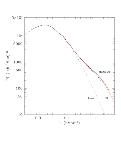
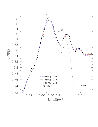
We study the convergence performance of the power spectra obtained with PPM-GLAM by comparing our results with those drawn from the high-resolution MultiDark simulations listed in Table 1. Specifically, we average power spectra of BigMDPL and HMDPL simulations weighted proportianally to the volume of each simulation. Left panel in Figure 1 shows the power spectra in $log-log$ scale for the A0.5 (red full curve), A1.5 (black dot-dashed) and A2.5 (blue dashed) PPM-GLAM simulations. As a reference we also show the linear power spectrum (dotted line).

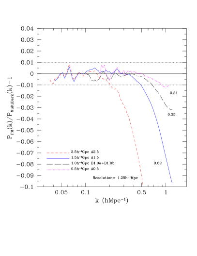
Our simulations closely reproduce well the clustering of the high-resolution MultiDark simulations (black full curve) both for long-waves (as may have been expected) and even for larger wave-numbers up to $k\approx 1\,h{\rm Mpc}^{-1}$ with exact deviations on larger $k$ depending on force resolution. The lack of force resolution results in the decline of the power spectrum at large wave-numbers: as resolution increases the power spectrum becomes closer to the MultiDark results. This is clearly seen in the left panel of Figure 2 where we show the ratios of the PPM power spectra $P(k)$ of A0.5 (red dot-dashed curve), A1.5 (blue full curve) and A2.5 (red dashed curve) to the power spectrum obtained from the MultiDark simulations. We also label in the plot the force resolution for each of the PPM-GLAM simulations. The results for the A0.5 simulations are presented only for $k>0.15\,h{\rm Mpc}^{-1}$ because the bin smearing becomes visible ($\sim 2$%) at lower frequencies due to the small volume of each individual realisation. We also plot the average of the B1.0a and B1.0b simulations (black long-dashed curve). Again, the deviations are less than 1% on large scales and they start to increase as we go to larger $k$ with the magnitude of the error depending on the force resolution. Note that the ratios of the PPM-GLAM results to those in the MultiDark simulations are the same at long-waves with $k<0.1\,h{\rm Mpc}^{-1}$. This is related with the cosmic variance present in the MultiDark $P(k)$ since there are only two realisations, i.e. BigMDPL and HMDPL.

The right panel in Figure 1 zooms-in on the relevant domain $k\approx 0.07-0.2\,h{\rm Mpc}^{-1}$ of the BAO peaks. In this plot the power spectrum $P(k)$ is multiplied by the factor $k^{5/4}$ to reduce the dynamical scale allowing us to see the differences as small as a fraction of percent. The cosmic variance of the PPM-GLAM simulations (errors of the mean) are nearly negligible because there are thousands of realisations. The observed deviations of the A0.5 points at small $k$ (e.g. $k\approx 0.08\,h{\rm Mpc}^{-1}$) are due to the large size of the binning in $k$ space defined by the width of the fundamental harmonic $\Delta k=2\pi/L=0.0125\,h{\rm Mpc}^{-1}$. If we consider simulations with small binning, i.e. simulation box $L\mbox{${\,\hbox{\hbox{$>$}\kern-8.00003pt\lower 4.30554pt\hbox{$\sim$}}\,}$}1\,\mbox{$h^{-1}$Gpc}$, then the deviations from the MultiDark simulations are less than 1 per cent on the large scales.

Figure 3: Comparison of power spectra in redshift-space at redshift zero. Monopole (left panel) and quadrupole (right panel) were scaled with different power of $k$ to reduce the dynamical range of the plots. The solid black curves correspond to the BigMDPL simulation estimated using 5% of all particles. The dashed curves and error bars are for the B1.5 simulations.

This is clearly seen in the left panel of Figure 2 were we show the ratios of GLAM power spectra to $P(k)$ in the MultiDark simulations. Results for the A0.5 simulations are presented only for $k>0.15\,h{\rm Mpc}^{-1}$ because the bin smearing becomes visible ($\sim 2$%) at lower frequencies. Again, the deviations are less than 1% on large scales and start to increase as we go to large $k$ with the magnitude of the error depending on the force resolution. Note that the ratios of the PM results to those in the MultiDark simulations are the same at $k<0.1\,h{\rm Mpc}^{-1}$. This is related with the cosmic variance in the MultiDark $P(k)$ – there are only two realizations of MultiDark.

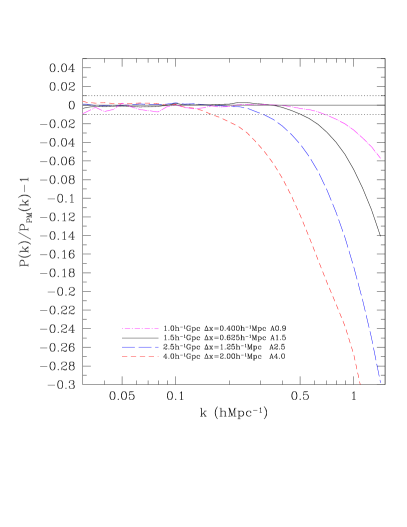
In order to test the effects of force resolution $\epsilon$ and finite box size $L$ we construct the combined power spectrum by taking the average of the best PPM-GLAM simulations in separate ranges of frequency: (1) for $k<0.1\,h{\rm Mpc}^{-1}$ we average $P(k)$ of all A1.5, A2.5, and A4.0 realisations, (2) for the range $0.1\,h{\rm Mpc}^{-1}<k<0.2\,h{\rm Mpc}^{-1}$ we take the average of the A2.5, A1.5, A0.9 simulations, (3) for $0.2\,h{\rm Mpc}^{-1}<k<0.4\,h{\rm Mpc}^{-1}$, A0.9 and A0.5 simulations are used, and (4) for larger wave-numbers we consider only the A0.5 realisations. We show in Figure 2 (right panel) the ratios of $P(k)$ of A0.9, A1.5, A2.5 and A4.0 simulations to the combined power spectrum. The deviations of each simulation from this combined $P_{\rm PM}(k)$ spectrum is a measure of the errors in each simulation. Note that these errors are broadly consistent with those of MultiDark except for the very long waves where we now do not have artificial deviations due to the cosmic variance. This plot gives us means to estimate what resolution is needed if we are required to provide some specified accuracy at a given scale. For example, if the errors in $P(k)$ should be less than 1% at $k<0.5\,h{\rm Mpc}^{-1}$, then the resolution of the simulation should be $\Delta x=0.62\mbox{$h^{-1}$Mpc}$. For, 1% at $k<1\,h{\rm Mpc}^{-1}$ the resolution should be $\Delta x=0.2\mbox{$h^{-1}$Mpc}$.

The right panel in Figure 2 also gives very useful information on the effects due to the finite box size. The size of the computational box is an important factor that affects the total CPU time, the statistics of the large-scale fluctuations, and possibly the non-linear coupling of long- and short waves. Non-linear coupling effects are of some concern (e.g., Gnedin et al., 2011; Li et al., 2014; Wagner et al., 2015; Baldauf et al., 2016) because the long-waves missed in small-box simulations (called Super Sample Covariance or SSC) can affect both the power spectrum and the covariance matrix. The magnitude of the SSC effect critically depends on the size of the computational box. Because our main target is relatively large boxes $L\approx(1-1.5)\,\mbox{$h^{-1}$Mpc}$ with high resolution, missing waves longer than these scales are deeply in the linear regime, and thus the SSC effects are expected to be small, which the right panel in Figure 2 clearly demonstrates.

The SSC effects should manifest themselves as an increase in $P(k)$ at small $k$ in simulations with large $L$ as compared with simulations with smaller $L$. Indeed, we see this effect at very long-waves. For example, at $k=0.03\,h{\rm Mpc}^{-1}$ the power spectrum in A0.5 simulations was below that of A4.0 by 4%. However, the effect becomes much smaller as the box size increases. The error becomes less than 0.2% for the A1.5 simulations. It is also much smaller for shorter waves. For example, the error is less than 0.5% for A0.9 simulations at $k>0.05\,h{\rm Mpc}^{-1}$. This can be understood if one estimates the amplitude of density fluctuations in waves longer than the simulation box. For $L=500\,\mbox{$h^{-1}$Mpc}$ and for the Planck cosmology the $rms$ density fluctuation $\delta(>L)$ is relatively large: $\delta(>500\,\mbox{$h^{-1}$Mpc})=0.027$. It is nearly ten times smaller for A1.5 simulations: $\delta(>1500\,\mbox{$h^{-1}$Mpc})=0.0036$.

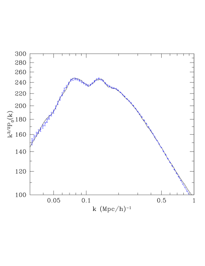
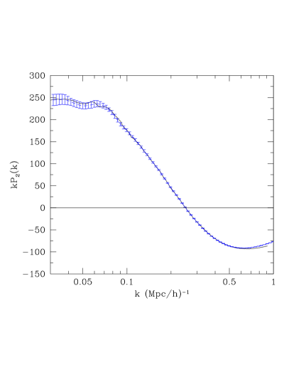
While the main interest of this paper is in the clustering in real-space, we also tested dark matter clustering in redshift-space and compared that with the MultiDark simulations. We plot in Figure 3 both monopole (left panel) and quadrupole (right panel) for PPM-GLAM B1.5 and BigMDPL, which shows a remarkable agreement.

5 Covariance Matrix.

Figure 4: Covariance matrix $C(k,k\prime)$ on logarithmic scale (left panel) and covariance coefficient $C(k,k\prime)/\sqrt{C(k,k)C(k\prime,k\prime)}$ (right panel) of the dark matter power spectrum at redshift zero for the PPM-GLAM A1.5 simulations. With the exception of the narrow spike at the diagonal of the matrix, the covariance matrix is a smooth function. Horizontal and vertical stripes seen in the correlation coefficient at small $k$ are due to cosmic variance.

The covariance matrix $C(k,k^{\prime})$ is defined as a reduced cross product of the power spectra at different wave-numbers for the same realisation averaged over different realisations, i.e.

$$C(k,k^{\prime})\equiv\langle P(k)P(k^{\prime})\rangle-\langle P(k)\rangle\langle P(k^{\prime})\rangle.$$ (8)

The diagonal and non-diagonal components of the covariance matrix have typically very different magnitudes and evolve differently with redshift. Their diagonal terms are larger than the off-diagonal ones, but there are many more off-diagonal terms making them cumulatively important (Taylor et al., 2013; Percival et al., 2014; O’Connell et al., 2016). Off-diagonal terms are solely due to non-linear clustering effects: in a statistical sense the off-diagonal terms are equal to zero in the linear regime. The diagonal component $C(k,k)$ can be written as a sum of the gaussian fluctuations due to the finite number of harmonics in a bin and terms that are due to non-linear growth of fluctuations:

$$C(k,k)\equiv C_{\rm Gauss}(k)+C_{\rm non}(k,k),$$ (9)

where the Gaussian term depend on the amplitude of the power spectrum $P(k)$ and on the number of harmonics $N_{h}$:

$$C_{\rm Gauss}(k)=\alpha\frac{2}{N_{h}}P^{2}(k),\quad N_{h}=\frac{4\pi k^{2}\Delta k}{\left(2\pi/L\right)^{3}},$$ (10)

where the numerical factor $\alpha$ is equal to unity for the Nearest-Grid-Point (NGP) assignment in Fourier-space and $\alpha=2/3$ for the CIC assignment used in this paper. Note that for a fixed bin width $\Delta k$ the number of harmonics, and thus, the amplitude of the Gaussian term scales proportional to the computational volume $N_{h}\propto L^{3}$ with $C_{\rm Gauss}(k)\propto 1/L^{3}$.

There are two ways of displaying the covariance matrix. One can normalise $C(k,k^{\prime})$ by its diagonal component: $r(k,k^{\prime})\equiv C(k,k^{\prime})/\sqrt{C(k,k)C(k^{\prime},k^{\prime})}$. This quantity is called the correlation coefficient, and by definition, $r(k,k)\equiv 1$. The covariance matrix can also be normalised by the ”signal”, i.e. the product of power spectra at the two involved wave-numbers: $\sqrt{C(k,k^{\prime})/P(k)P(k^{\prime})}$.

Figure 5: Diagonal components of the covariance matrix for PPM-GLAM simulations with different box sizes at $z=0$ (left panel), and for different redshifts for the A0.9 simulations (right panel). All results were rescaled to the simulation volume of $1.5\mbox{$h^{-1}$Gpc}$. The dotted lines show the Gaussian contribution $C_{\rm Gauss}$ given by eq. (10) with $\alpha=2/3$, which gives a good approximation up to $k\mbox{${\,\hbox{\hbox{$<$}\kern-8.00003pt\lower 4.30554pt\hbox{$\sim$}}\,}$}0.2\,h{\rm Mpc}^{-1}$. At larger wave-numbers the covariance matrix is substantially larger than the Gaussian term due to the non-linear coupling of waves. The diagonal terms evolve with redshift and sensitively depend on the force resolution.

Figure 6: Slices through the $z=0$ covariance matrix $C(k,k\prime)$ at different values of $k^{\prime}$ for $\sim 4500$ realisations of PPM-GLAM A1.5. Left: Covariance coefficient $C(k,k\prime)/[C(k,k)C(k\prime,k\prime)]^{1/2}$ (top panel) and covariance matrix normalised to the power spectrum $[C(k,k\prime)/P(k)P(k^{\prime})]^{1/2}$ (bottom panel) for $k^{\prime}=0.12,0.2,0.3,0.5\,{\rm h\,{\rm Mpc}}^{-1}$. Note the change in scale of the y-axes. The covariance matrix normalised by the signal is very small $\sim 3\times 10^{-3}$ and relatively flat as compared with the large differences seen in the covariance coefficients on the top panel. Right: Detailed views of the covariance matrix. Solid curves with the error bars are for the A1.5 simulations. Results for the A0.9 simulations scaled to the 1.5$h^{-1}$Gpc volumes are shown with dashed curves. Dotted curves show the analytical approximation given in Eqs. (11-13). As $k$ increases the covariance matrix first decreases, reaches the minimum at $k\approx(0.1-0.2)h\,{\rm Mpc}^{-1}$ and then has a maximum at $k\approx(0.5-0.6)h\,{\rm Mpc}^{-1}$. In addition, it has a dip on both sides of the diagonal components.

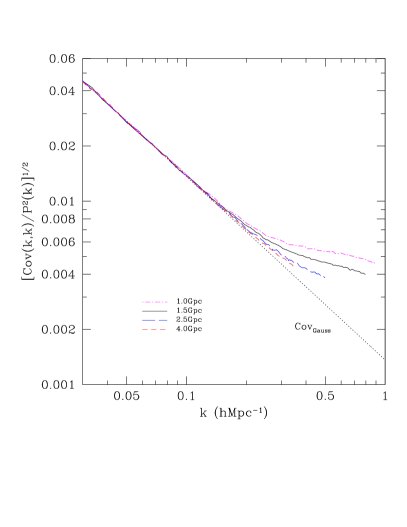
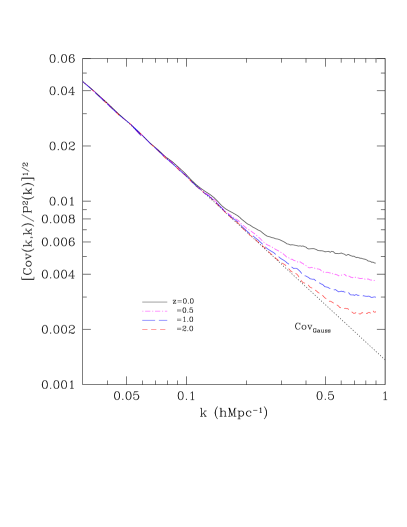
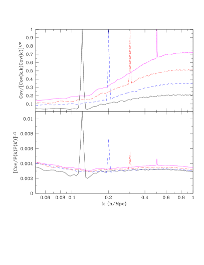
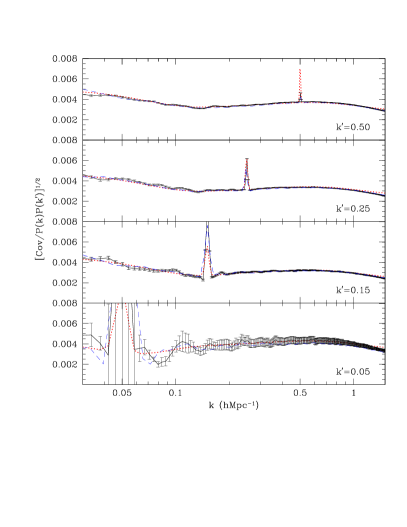
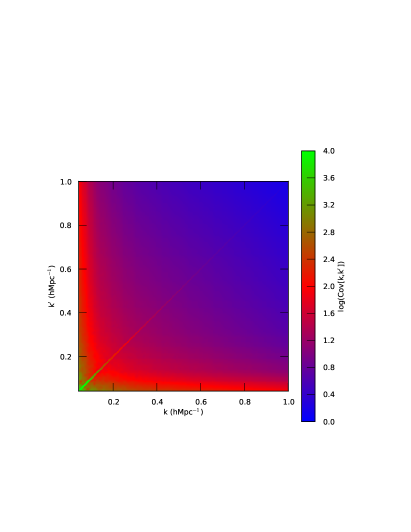
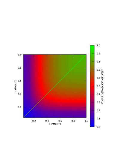
Figure 4 shows the covariance matrix $C(k,k^{\prime})$ and the correlation coefficient for the PPM-GLAM A1.5 simulations at $z=0$. With the exception of a narrow spike at the diagonal of the matrix, the covariance matrix is a smooth function. Horizontal and vertical stripes seen in the correlation coefficient at small $k$ are due to cosmic variance. They gradually become weaker as the number of realisations increases (e.g., Blot et al., 2015).

The diagonal terms of the covariance matrix are presented in Figure 5. In the left panel we compare the results of various simulations at $z=0$ with different box sizes. In order to do that, we rescale the individual $C(k,k)$ to that of the volume of the A1.5 simulation with $(1.5\mbox{$h^{-1}$Gpc})^{3}$. Up to $k\mbox{${\,\hbox{\hbox{$<$}\kern-8.00003pt\lower 4.30554pt\hbox{$\sim$}}\,}$}0.2\,h{\rm Mpc}^{-1}$ the covariance matrix is well described by the Gaussian term, but at larger wave-numbers it substantially exceeds the Gaussian contribution due to the non-linear coupling of waves. The force resolution plays an important role here.

There are no indications that SSC waves (modes longer than the simulation box) affect the diagonal components. If present, SSC effects should results in enhanced $C(k,k)$ in simulations with very large simulation boxes (Li et al., 2014; Baldauf et al., 2016). For example, A4.0 results should have a larger covariance matrix as compared with that of the A0.9 simulations. However, the right panel of Figure 5 clearly shows the opposite effect: A0.9 results are above A4.0 presumably due to the better force resolution that produces larger non-linear effects.

Figure 7: Evolution of the covariance matrix with redshift for $k^{\prime}=0.2\,{\rm h\,Mpc}^{-1}$ in the A1.5 simulations. Top and bottom panels show the covariance coefficient and the covariance matrix normalised to the power spectra. Curves on the right panels were scaled up with the linear growth factor $\delta(t)$. Results indicate that at very long waves $k\mbox{${\,\hbox{\hbox{$<$}\kern-8.00003pt\lower 4.30554pt\hbox{$\sim$}}\,}$}0.07\,{\rm h\,Mpc}^{-1}$ the covariance matrix grows very fast as $C\propto\delta(t)P(k,t)P(k^{\prime},t)\propto\delta^{5}(t)$. At intermediate wave-numbers $0.1\,{\rm h\,Mpc}^{-1}<k<0.5\,{\rm h\,Mpc}^{-1}$ the growth is even faster $C\propto\delta^{5.25}(t)$.

Figure 8: Dependance of the covariance matrix on box size. PPM-GLAM simulations with three box sizes are used: $L=0.5\mbox{$h^{-1}$Gpc}$  (A0.5), 1.5$h^{-1}$Gpc  (A1.5), and 2.5$h^{-1}$Gpc  (A2.5). In all cases the binning of the power spectra is defined by the fundamental harmonic $\Delta k=2\pi/L$ resulting in the finest binning and largest noise in the biggest box. Left: The unscaled covariance matrix dramatically declines with increasing $L$. Right: Covariance matrices of the A0.5, A1.5 and A4.0 simulations are scaled to the same volume of $1.5\mbox{$h^{-1}$Gpc}$.

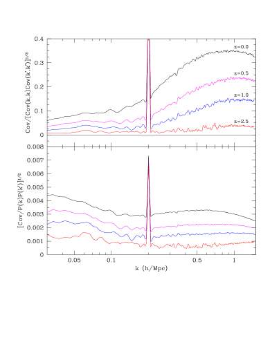
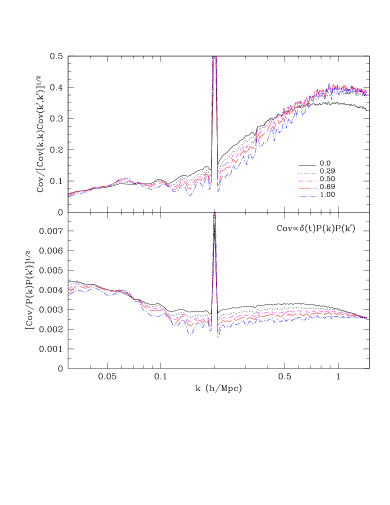
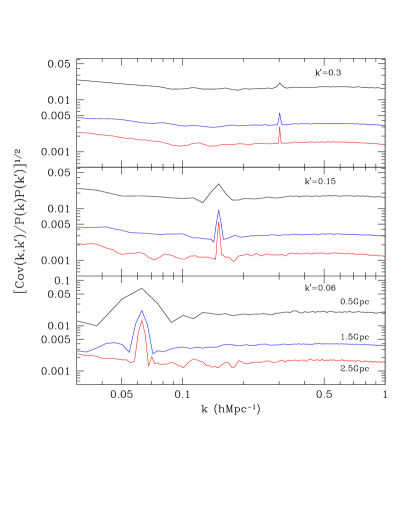
Figures 6 and 7 demonstrate that the non-diagonal terms of the covariance matrix have a complex structure. They depend on both $k$ and $k^{\prime}$ in a non-trivial way and they evolve with redshift in a complicated fashion. The bottom left panel in Figure 6 highlights one of the main issues with the non-diagonal terms: each term is small $\sim 3\times 10^{-3}$ as compared with the signal, but there are many of them. The fact that individual components are so small is one of the reasons why one needs thousands of realisations to estimate the covariance matrix reliably.

However, with the exception of the diagonal componentes, the covariance matrix is a smooth function that can be approximated analytically using a relatively small number of parameters. The following approximation gives 3% accuracy for the $z=0$ covariance matrix at $k\mbox{${\,\hbox{\hbox{$>$}\kern-8.00003pt\lower 4.30554pt\hbox{$\sim$}}\,}$}0.1\,h{\rm Mpc}^{-1}$ and $\sim 10\%$ at smaller wave-numbers:

$$C(k,k^{\prime}) = 8.64\times 10^{-6}L^{-3}P(k)P(k^{\prime})$$

$$\times \left[1+g(k)+g(k^{\prime})\right]^{2}$$

$$\times \left[1-\alpha e^{-\frac{(k-k^{\prime})^{2}}{2\sigma^{2}}}+(1+\alpha)e^{-\frac{(k-k^{\prime})^{2}}{2(0.1\sigma)^{2}}}\right]^{2},$$

where

$$g(k)=1.4\exp\left[-\left(\frac{k}{0.07}\right)^{2}\right]+\frac{1.1k^{0.60}}{1+1.2k^{3}},$$ (12)

and

$$\alpha=0.03/k^{\prime},\qquad\sigma=4\kappa=4(2\times 10^{-3}\pi/L).$$ (13)

Here the box size $L$ is in units of $h^{-1}$Gpc and wave-numbers are in units of $h\,{\rm Mpc}^{-1}$. In spite of the fact that the fit has 10 free-parameters, it is still a useful approximation.

The approximation for $C(k,k^{\prime})$ is so complicated because the covariance matrix has a complex dependence on $k$ and $k^{\prime}$. For a fixed $k^{\prime}$ the covariance matrix declines with increasing $k$. For example, the covariance matrix declines by a factor of $\sim 2.5$ from $k=0.03\,h{\rm Mpc}^{-1}$ as compared to $k=0.1\,h{\rm Mpc}^{-1}$. It reaches a flat minimum at $k\approx(0.1-0.2)h\,{\rm Mpc}^{-1}$ and then increases by factor $~{}1.5$ and reaches a maximum at $k\approx(0.5-0.6)h\,{\rm Mpc}^{-1}$. In addition, it has a dip on both sides of the diagonal components (see Figure 6), which is approximated by the last terms in eq. (LABEL:eq:fit1).

The approximation given by eqs. (LABEL:eq:fit1-13) are only for the non-diagonal components of $C(k,k^{\prime})$. For the diagonal components the fallowing approximation gives a $\sim 2\%$-accurate fit to the A0.9 simulations:

$$C(k,k)=P^{2}(k)\left[\alpha\frac{2}{N_{h}}+A^{2}\right],$$ (14)

where parameter $A$ is a slowly increasing function of wave-number:

$$A=\frac{5.5\times 10^{-3}}{L^{3/2}}\left[1+\left(\frac{k}{1.5}\right)^{1/2}-\frac{k}{4}\right],\quad k<1\,h{\rm Mpc}^{-1}.$$ (15)

The evolution of the covariance matrix with redshift is equally complex as that illustrated in Figure 7 that shows $C(k,k^{\prime})$ for the A1.5 simulations at different redshifts. Curves on the right panels were scaled up with the linear growth factor $\delta(t)$. Results indicate that on very long waves $k\mbox{${\,\hbox{\hbox{$<$}\kern-8.00003pt\lower 4.30554pt\hbox{$\sim$}}\,}$}0.07\,{\rm h\,Mpc}^{-1}$ the covariance matrix grows very fast as $C\propto\delta(t)P(k,t)P(k^{\prime},t)\propto\delta^{5}(t)$. At the intermediate scales $0.1\,{\rm h\,Mpc}^{-1}<k<0.5\,{\rm h\,Mpc}^{-1}$ the growth is even faster: $C\propto\delta^{5.25}(t)$

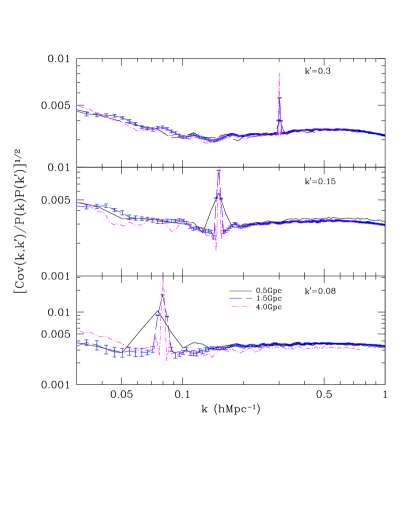
We also conclude that the covariance matrix decreases with the increasing computational volume. We already saw it for the diagonal components. The same is true for the non-diagonal terms as illustrated by the left panels in Figure 8. The scaling of the whole covariance matrix with volume is trivial: $C\propto L^{-3}$. It is not an approximation or a fit. It is a scaling law. Right panels in the figure show the results for $C$ rescaled to the $(1.5\mbox{$h^{-1}$Gpc})^{3}$ volume of the A1.5 simulations. This is an important scaling, which is often forgotten. Errors in the estimates of the power spectrum of fluctuations (and thus the errors in cosmological parameters) would have been too large if one were to stack together many small simulations to mimic large observational volume and forget to re-scale the covariance matrix. However, when the rescaling is done, the small-box simulations perfectly reproduce the clustering signal and statistics of much larger simulations.

6 Comparison with other results

The speed of $N$-body simulations is very critical for the generation of mock galaxy samples – the ultimate goal for the GLAM project. Computational timings of some PM codes are available (Izard et al., 2015; Feng et al., 2016; Koda et al., 2016), but those timings are performed for different configurations, i.e. different number of particles, mesh-sizes, time-steps, and computing facilities. Fortunately, rescaling of the timings can be done because most of the results are relatively recent (and use similar Intel processors). Most of the CPU is used for numerous FFTs. So, results can be rescaled to the same configuration. We re-scale all relevant numbers to a hypothetical simulation with $\mbox{$N_{\rm p}$}=1000$, $\mbox{$N_{\rm g}$}=3000$, and the number of time-steps $\mbox{$N_{\rm s}$}=150$. Table 2 presents the CPU and memory required to run such a simulation with different codes.

Table 2: Rescaled CPU and memory required by different PM codes to make one 150 time-steps simulation with 1 billion particles and $\mbox{$N_{\rm g}$}=3000$ mesh.

	GLAM	COLA1	ICE-COLA2	FastPM3
CPU, hrs	146	220	320	567
Memory, Gb	123	240	325	280
1Koda et al. (2016), 2Izard et al. (2015), 3Feng et al. (2016)

So far PPM-GLAM code is the fastest available code for this type of simulations: it is a factor of 2-3 faster than some other codes and it requires significantly less memory. This is not surprising considering GLAM’s simplicity and efficiency. The code is particularly tuned for production of thousands of realisations. Indeed, it is trivially parallelised with MPI library calls to run hundreds of realisations at a time, which is exactly what we have done. It also has an advantage that it can be used on a small cluster or on a single computing node without installed MPI library. It has a disadvantage that it is limited by the memory available on a single node.

It is interesting to note that approximate methods for the generation of a large number of galaxy/halo mock catalogs (see Chuang et al., 2015) , while promising fast and cheap production of thousands of catalogs, may not be very efficient and fast as one may imagine. For example, Kitaura et al. (2016) generated $12,288$ mock catalogs for the BOSS galaxy survey Kitaura et al. (2016) using the PATCHY-code (Kitaura & Heß, 2013), which is based on a combination of second-order perturbation theory and spherical infall model (ALPT). The results are very valuable for the project and score really well when compared with other methods as those discussed in Chuang et al. (2015). The code uses a $960^{3}$ mesh, $2.5\mbox{$h^{-1}$Gpc}$ box and spatial resolution of $2.6\mbox{$h^{-1}$Mpc}$. It produced $40,960$ realisations with 12.2 CPU-hours and 24 Gb RAM per realisation. That seems to be very fast when one compares it with ICE-COLA which requires 2.6 Tb of RAM and 1000 CPU hours (Izard et al., 2015).

However, this is a misleading comparison because the resolution of the ICE-COLA simulations is $0.25\mbox{$h^{-1}$Mpc}$ – ten times better than PATCHY, and COLA does not use inaccurate spherical collapse model. In order to make a fair comparison, we estimate the CPU time needed for PPM-GLAM to make a realisation with the the same box size, $960^{3}$ mesh and force resolution of $2.6\mbox{$h^{-1}$Mpc}$ as in PATCHY. We assume that 40 time-steps would be sufficient for this resolution (see eq. (41)) and use $(960/2)^{3}$ particles. The CPU time to make one $N-$body simulation with PPM-GLAM is 1.4 CPU-hours, which is smaller that for PATCHY. One simulation with PPM-GLAM will also require about 4 times less memory than what is needed for a PATCHY mock. In other words, it is faster and more accurate to make one $N-$body simulation than use the approximate PATCHY gravity solver.

Our results on convergence of the power spectrum are very similar to those presented in Izard et al. (2015) for their ICE-COLA simulations. Their Figure 6 indicates that 1% error in the power spectrum $P(k)$ is reached at $k\approx 0.7-0.8\,h{\rm Mpc}^{-1}$ for a simulation with $\Delta x=0.25\mbox{$h^{-1}$Mpc}$. Our Figure 2 shows that 1% error at $k\approx 0.7\,h{\rm Mpc}^{-1}$ occurs for our PPM-GLAM simulation with a similar resolution of $\Delta x=0.35\mbox{$h^{-1}$Mpc}$. Convergence of the power spectrum is somewhat worse for the FastPM code (Feng et al., 2016): For the force resolution of $\Delta x=0.225\mbox{$h^{-1}$Mpc}$ they reach 1% error in $P(k)$ only at $k\approx 0.3\,h{\rm Mpc}^{-1}$. At $k\approx 0.7\,h{\rm Mpc}^{-1}$ the error is 2% for the FastPM simulations. Note that it should have been other way around because FastPM has a bit better force resolution and should have better accuracy. It is not clear what causes this discrepancy.

Results on the covariance matrix of the dark matter power spectrum are more difficult to compare because the covariance matrix depends sensitively on cosmological parameters and has a complicated shape. Some publications claim that, once the Gaussian diagonal terms are removed, the covariance function is a constant: $C(k,k^{\prime})=\delta(k-k^{\prime})\,C_{\rm Gauss}(k)+\sigma^{2}P(k)P(k^{\prime})$ (Neyrinck, 2011; Mohammed & Seljak, 2014; Carron et al., 2015). This simple model is not consistent with our results as presented in Figure 8. The main difference is the upturn of $C(k,k^{\prime})$ at $k<0.1\,h{\rm Mpc}^{-1}$ where the covariance matrix changes quite substantially. For example, $C(k,k^{\prime})/P(k)P(k^{\prime})$ changes by a factor of two from $k^{\prime}=0.15\,h{\rm Mpc}^{-1}$ down to $k^{\prime}=0.03\,h{\rm Mpc}^{-1}$. Even at larger wave-numbers there is clear increase with increasing $k$, though this effect is not that large ($\sim 20\%$).

Recently, Blot et al. (2015) and Li et al. (2014) presented covariance matrices for a large set of $N$-body simulations. It is difficult to compare our results with those of Blot et al. (2015) because of the large differences in cosmological parameters. However, the differences are smaller for Li et al. (2014). By comparing our covariance matrix for PPM-GLAM A0.5 simulations with Li et al. (2014), as presented in Figure 1 of Bertolini et al. (2016) and Figure 8 of Mohammed et al. (2016), we find that our results are within $\sim 10\%$ of Li et al. (2014). However, there are some differences when we use our full set of simulations. For example, we clearly find the gradual increase in $C(k,k^{\prime})$ with increasing $k$ for $k>0.1\,h{\rm Mpc}^{-1}$ and subsequent decline (see right panel in Figure 8). The results of Li et al. (2014) are inconclusive in this matter.

Li et al. (2014) presented simulations only for a relatively small $500\mbox{$h^{-1}$Mpc}$ computation box. Instead, we study the covariance matrix for vastly different box sizes, which allows us to asses effects of SSC modes. We find very little effect of SSC on $C(k,k^{\prime})$.

7 Conclusions

Making accurate theoretical predictions for the clustering statistics of large-scale galaxy surveys is a very relevant but complicated physical process. In this paper we present and discuss our results on a number of important aspects. Some of them are technical (e.g., convergence of the power spectrum) and others are of vital importance for the properties of the dark matter density field that affects directly the inference of cosmological parameters from large galaxy catalogs (e.g. covariance matrices). There are different paths to producing mock galaxy catalogs where the predictions for the dark matter clustering and dynamics is a crucial stage of this process. Only after the dark matter distribution is approximated one way or another, and its clustering properties are reliable and accurate, we can then build the next step of connecting dark matter with galaxies, which will be subject of our forthcoming work.

The properties of the dark matter covariance matrix have been studied using numerical simulations (Takahashi et al., 2009; Li et al., 2014; Blot et al., 2015) or analytical methods (Mohammed & Seljak, 2014; Bertolini et al., 2016; Carron et al., 2015; Mohammed et al., 2016). Here we present a detailed analysis of the covariance matrix based on a very large set of $N$-body simulations that cover a wide range of numerical and cosmological parameters. We study the structure, evolution, and dependance on numerous numerical effects of the dark matter covariance matrix using a new Parallel Particle-Mesh code, named PPM-GLAM. Contrary to some previous results (e.g., Neyrinck, 2011; Mohammed & Seljak, 2014) we find that the covariance matrix $C(k,k^{\prime})$ is a very complicated entity with complex dependance on wave-numbers $k$ and $k^{\prime}$. We provide accurate approximations in eqs. (LABEL:eq:fit1-15) of the covariance matrix at $z=0$ for the standard $\Lambda$CDM model with Planck parameters.

The covariance matrix evolves with redshift. It grows linearly for very long waves: $C(k,k^{\prime})/P(k)P(k^{\prime})\propto\delta(z)$, where $\delta(z)$ is the linear growth factor. At larger wave-numbers it growths faster with $C(k,k^{\prime})/P(k)P(k^{\prime})\propto\delta^{5/4}(z)$. The fast growth of the covariance matrix implies that $C(k,k^{\prime}))$ must depend on the overall normalisation $\sigma_{8}$ of the power spectrum and very likely on other cosmological parameters. This is hardly surprising considering that the power spectrum – second order clustering statistics – depends on cosmology. Why the third-order statistics such as the covariance matrix would not?

We use vastly different simulation volumes to study the effects of SSC waves – waves longer than the simulation box. We clearly see these effects in the power spectrum $P(k)$, but they occur only on very small wave-numbers $k\mbox{${\,\hbox{\hbox{$<$}\kern-8.00003pt\lower 4.30554pt\hbox{$\sim$}}\,}$}0.03\,h{\rm Mpc}^{-1}$ and only for small simulation boxes $L\mbox{${\,\hbox{\hbox{$<$}\kern-8.00003pt\lower 4.30554pt\hbox{$\sim$}}\,}$}500\mbox{$h^{-1}$Mpc}$. There are no detectable SSC effects for simulation boxes $L=1.5\mbox{$h^{-1}$Gpc}$.

Figure 9: Dependance of the different numerical parameters of the PPM-GLAM simulations on box- and mesh-size. The vertical lines at the top-axis of the plot show the computer memory required for a simulation with mesh-size $N_{\rm grid}$ and number of particles $\mbox{$N_{\rm p}$}=N_{\rm grid}/2$. Dot-dashed lines correspond to the number of CPU-hours needed to make a single realisation with the given combination of mesh-size (and particles) and number of steps as defined by eq. (17). Diagonal dotted (blue) lines show constant values of $k_{1\%}$ (the wave-number at which the error in $P(k)$ reaches the level of 1%). In order to achieve better resolution than a selected value of $k_{1\%}$, the simulation parameters (box- and mesh-size) should be set to those values located below the corresponding $k_{1\%}$ dotted line. Dashed (red) lines are lines of constant CPU time (in hours) required to make a set of PPM-GLAM simulations with the cumulative volume of $5000\,(\mbox{$h^{-1}$Gpc})^{3}$. In order to avoid large Super Sample Covariance (SSC) defects, the simulations should have large enough box-size $L>\mbox{${\,\hbox{\hbox{$>$}\kern-8.00003pt\lower 4.30554pt\hbox{$\sim$}}\,}$}500\,\mbox{$h^{-1}$Mpc}$. The requirements to have a large number of realisations $N_{\rm r}$, for a given CPU time and accuracy, tend to reduce the simulation box-size. Overall, these different constraints tend to limit the selection of computational parameters to the oval area indicated in the plot. Open circles corresponds to the PPM-GLAM simulations listed in Table 1 and used in our analysis.

The optimum selection of the computational volume of $N$-body simulations to estimate covariance matrices requires special attention because it potentially can change the accuracy of the covariance matrix and power spectrum. It definitely affects the required CPU time and requested memory. With increasing volume of observational samples, one naively expects that the computational volume of an individual mock catalog also must increase, and thus, cover the whole survey volume (e.g. Monaco, 2016, and references therein). Yet, this is not necessarily correct. Weak-lensing samples still cover relatively small volumes and in this case using simulations that cover the observed samples may be vulnerable to large SSC effects. So, much larger computational boxes may be required.

At the same time, the very large survey volumes of e.g. DESI (DESI Collaboration et al., 2016) and Euclid (Laureijs et al., 2011) may not require equally large simulation volumes. We argue that one can replicate (stack) a smaller but still significant simulation box as many times as needed to cover the larger observational volume and on this way to produce a viable mock galaxy catalog. As long as we are only interested in a quantity (e.g., power spectrum or correlation function) that is defined on scales significantly smaller than the computational volume, there should be no defects. Indeed, Figure 2 shows that the power spectrum is not affected by the simulation box. The covariance matrix is not affected either after it is scaled down by the ratio of the observational volume to the volume of the simulation. Indeed, we already saw that the covariance matrix scales proportionally to the volume (see, eqs. (LABEL:eq:fit1 - 15) and Figure 8). For example, for the analysis of BAO peaks and scales of $\sim 100\,\mbox{$h^{-1}$Mpc}$ a simulation box of size $L\approx(1-1.5)\mbox{$h^{-1}$Mpc}$ is a good choice.

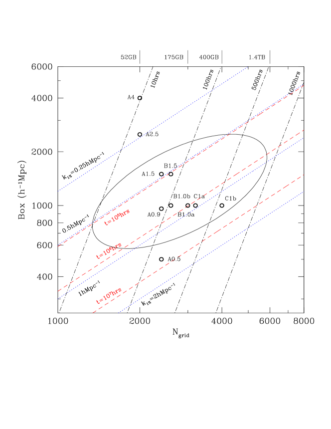
Finally, we estimate the computational resources – CPU time and computer memory – required to run a large set of PPM-GLAM simulations for different combinations of box size $L$, accuracy of the power spectrum and mesh size $N_{\rm g}$. There are many factors that define the optimal selection of computational parameters, including the number of time-steps, the number of realisations, the effects of super-sample waves and the limitations on the available computer memory. Using the results presented in this paper on the errors in the power spectrum (see Figures 2 and 12) we provide estimates for (i) the wave-number $k_{1\%}$ at witch the error in $P(k)$ reaches the level of 1%:

$$k_{1\%}=\frac{0.3}{\Delta x}=\frac{0.3\mbox{$N_{\rm g}$}}{L},$$ (16)

where the box size $L$ is given in units of $h^{-1}$Mpc. Lines of constant $k_{1\%}$ are shown as dotted (blue) lines in Figure 9. The larger the value of $k_{1\%}$, better is the performance reached at smaller scales. (ii) to estimate the number of time-steps $N_{\rm s}$ required for a given simulation, we assume that on average the particles should not move more than $1/3$ of a cell. This includes fast-moving particles in clusters of galaxies. We assume that the $rms$ 3D-velocity for the particles in galaxy clusters is $v\approx 2000\,\mbox{$\rm{km\,sec}^{-1}$ }$. Estimating the number of steps as $a/\Delta a=\mbox{$N_{\rm s}$}$ and using eq. (41) with $\beta=1/3$, we find that the number of time-steps is

$$\mbox{$N_{\rm s}$}\approx\frac{60\mbox{$N_{\rm g}$}}{L},$$ (17)

where the box size is given in units of $h^{-1}$Mpc.

Thus, the total amount of CPU-hours required for producing $N_{r}$ simulations with box size $L$ and mesh size $N_{\rm g}$ is

$$t_{\rm tot}=N_{r}\mbox{$N_{\rm s}$}\mbox{$N_{\rm g}$}^{3}t_{1}=2.4\times 10^{-9}N_{r}N_{g}^{4}L^{-1},$$ (18)

where $t_{1}$ is the CPU-hours required per time-step. Here we use the timings provided in the first raw of Table 3. It is also convenient to use the total volume covered by all set of realisations, i.e. $V=N_{r}L^{3}$. Using the expressions for the total volume and CPU-hours, $V$ and $t_{\rm tot}$, we can write a relation between the required box size $L$ and grid $N_{\rm g}$ to run many simulations covering a volume $V$ under the condition that the total CPU is $t_{\rm tot}$:

$$L=\left(\frac{2.4\times 10^{-9}V}{t_{\rm tot}}\right)^{1/4}\mbox{$N_{\rm g}$}.$$ (19)

In Figure 9 we plot lines of $L(\mbox{$N_{\rm g}$})$ for a somewhat arbitrary value of $V=5000(\mbox{$h^{-1}$Gpc})^{3}$ and for three different CPU times of $10^{5},10^{6},10^{7}$CPU-hours. Additional constraints are coming from the SSC modes that limit the box size, which we assume to be bigger than $L=500\,\mbox{$h^{-1}$Mpc}$. The number of realisations should be large (thousands) regardless of the total covered volume. This tends to limit the box size to lower values, or, equivalently, to increase proportionally the CPU time. All theses limitations are shown in Figure 9. They indicate that currently the selection is limited to the parameters inside the oval drawn in the plot.

The results presented in this work demonstrate that the Parallel Particle-Mesh GLAM code, at a very low computational cost, generates the accurate dark matter clustering statistics required for the production of thousands of mock galaxy catalogs. The next step, which will be presented in a future paper, will be to develop a bias scheme that will take as input the accurate density field provided by PPM-GLAM and produce those large galaxy catalogs in the context of the upcoming and existing large-scale galaxy surveys.

Appendix A The PPM-GLAM code

In general, a cosmological PM code consists of three steps to evolve the particles: (1) Using the particle positions $\bf r$ to obtain the density $\rho_{i,j,k}$ at the nodes of an homogenous 3D-mesh that covers the computational domain, (2) Solve the Poisson equation on the mesh, and (3) advance the particles to a new moment of time.

A.1 Density field:

We start with the calculation of the density field produced by $N_{\rm p}^{3}$ particles on the $N_{\rm g}^{3}$ nodes of the mesh. In order to assign the particle density to the 3D-mesh, we introduce a particle shape (Hockney & Eastwood, 1988). If $S(x)$ is the density at distance $x$ from the particle and $\Delta x$ is the cell size, then the density at distance $(x,y,z)$ is the product $S(x)S(y)S(z)$. Two choices for $S$ are adopted: Cloud-In-Cell (CIC) and Triangular Shaped Cloud (TSC). Here we will use the CIC scheme, i.e.

$$CIC:S(x)=\frac{1}{\Delta x}\begin{cases}1,\,|x|<\Delta x/2\\ 0,\,{\rm otherwise}\end{cases}.$$ (20)

The fraction of particle mass assigned to a cell is just a product of three weight functions $w(x)w(y)w(z)$, where $\bf r=\bf r_{p}-\bf x_{i}$ is the distance between particles with coordinates $\bf x_{p}$ and cell center $\bf x_{i}$. The weight function is $w(x)=\int^{x_{i}+\Delta/2}_{x_{i}-\Delta/2}S(x_{p}-x^{\prime})dx^{\prime}$:

$$CIC:w(x)=\begin{cases}1-|x|/\Delta x,\,|x|<\Delta x\\ 0,\phantom{mmmmm}{\rm otherwise}\end{cases}.\phantom{mmmmmmmm}$$ (21)

Although these relations given in eqs.(20–21) look somewhat complicated, in reality they require very few operations in the code. For the CIC scheme a particle contributes to the 8 nearest cells. If the coordinates are scaled to be from $0$ to $N_{\rm g}$, where $N_{\rm g}$ is the size of the grid in each direction, then taking an integer part of each particle coordinate with center $(x,y,z)$ - in Fortran: $i=INT(x)...$ - gives the lower bottom grid cell $(i,j,k)$. Then, the distance of the particle from that cell center is $dx=x-i,dy=y-j,dz=z-k$.

A.2 Gravitational potential

Having the density field $\rho_{i,j,k}$, we can estimate the gravitational potential by solving the Poisson equation, which for clarity we simply write as

$$\nabla^{2}\phi=4\pi G\rho(\bf x).$$ (22)

We start with applying a 3D Fast Fourier Transformation (FFT) to the density field. That gives us the Fourier components on the same grid $\tilde{\rho}_{\bf k}$, where $\bf k$ is a vector with integer components in the range $0,1,\dots,N_{\rm g}-1$. Now we multiply the harmonics $\tilde{\rho}_{i,j,k}$ by the Green functions $G(\bf k)$ to obtain the Fourier harmonic amplitudes of the gravitational potential $\phi$, i.e.

$$\tilde{\phi}_{i,j,k}=4\pi G\tilde{\rho}_{i,j,k}G(\bf k),$$ (23)

and then do the inverse FFT to find out the gravitational potential $\phi_{i,j,k}$. Note that all these operations can be organized in such a way that only one 3D-mesh is used – no additional RAM memory is required.

The simplest, but not the best, method to derive the Green functions is to consider $\phi_{i,j,k}$ and $\rho_{i,j,k}$ as amplitudes of the Fourier decomposition of the gravitational potential in the computational volume, and then to differentiate the Fourier harmonics analytically. This gives

$$G_{0}(\bf k)=-\frac{1}{k_{x}^{2}+k_{y}^{2}+k_{z}^{2}}=-\left(\frac{L}{2\pi}\right)^{2}\frac{1}{i^{2}+j^{2}+k^{2}}.$$ (24)

A better way of solving the Poisson equation that we use in our PPM-GLAM code is to start with the finite-difference approximation of the Laplacian $\nabla^{2}$. Here we use a the second order Taylor expansion for the spacial derivatives:

$$\nabla^{2}\phi = \frac{\partial^{2}\phi}{\partial x^{2}}+\frac{\partial^{2}\phi}{\partial y^{2}}+\frac{\partial^{2}\phi}{\partial z^{2}}$$

$$\approx [\phi_{i+1,j,k}-2\phi_{i,j,k}+\phi_{i-1,j,k}$$

$$+ \phi_{i,j+1,k}-2\phi_{i,j,k}+\phi_{i,j-1,k}$$

$$+ \phi_{,j,k+1}-2\phi_{i,j,k}+\phi_{i,j,k-1}]/\Delta x^{2}.$$

This approximation leads to a large system of linear algebraic equations: $A\phi=4\pi G\rho$, where $\rho$ is the vector on the right hand side, $\phi$ is the solution, and $A$ is the matrix of the coefficients. All of its diagonal components are equal to -6, and all 6 nearest off-diagonal components are 1. The solution of this matrix equation can be found by applying the Fourier Transformation. This provides another approximation for the Green functions:

$$G_{1}(\bf k)=\frac{\Delta x^{2}}{2}\left[\cos\left(\frac{2\pi i}{N_{\rm g}}\right)+\cos\left(\frac{2\pi j}{N_{\rm g}}\right)+\cos\left(\frac{2\pi k}{N_{\rm g}}\right)-3\right]^{-1}.$$ (26)

For small $(i,j,k)$, eq.(26) gives the same results as eq.(23). However, when $(i,j,k)$ is close to $N_{\rm g}$, the finite-difference scheme $G_{1}$ provides less suppression for high-frequency harmonics and thus gives a stronger and more accurate force at distances closer to the grid spacing $\Delta x$. Hockney & Eastwood (1988) argue that this happens because the finite-difference approximation partially compensates the dumping of short waves that are related with the density assignment.

A.3 Time-stepping

We write the particle equations of motions and the Poisson equation, using the particle momenta ${\mn@boldsymbol{p}}\equiv a^{2}\dot{{\mn@boldsymbol{x}}}$, as follows

$$\frac{d\bf x}{da} = {\bf u},\qquad{\bf u}\equiv\frac{{\bf p}}{a^{3}H},\quad{\mn@boldsymbol{p}}\equiv a^{2}\dot{{\mn@boldsymbol{x}}},$$ (27)

$$\frac{d\bf p}{da} = {\bf g},\qquad{\bf g}\equiv-\frac{\nabla\phi}{aH},$$ (28)

$$\nabla^{2}\phi = \frac{3}{2}\frac{H_{0}^{2}\Omega_{0}\delta_{\rm dm}}{a},$$ (29)

$$H^{2} = H_{0}^{2}\left(\frac{\Omega_{0}}{a^{3}}+\Omega_{\Lambda,0}\right),\quad\Omega_{0}+\Omega_{\Lambda,0}=1.$$ (30)

Here we specifically assumed a flat $\Lambda CDM$ cosmological model with the cosmological constant characterised by the density parameter $\Omega_{\Lambda,0}$ at redshift $z=0$.

Because we start the simulations at a relatively high redshift $z_{i}\approx 100$, and because the number of time-steps $N_{s}\approx 100-200$ is not large, the time-stepping scheme should be carefully selected and tuned. In the sense of the accuracy of the time-stepping algorithms, there are two regimes: (1) when fluctuations grow nearly linearly at large redshifts and when the expansion factor $a$ may change substantially over a single time-step, and (2) later moments when fluctuations are in the non-linear regime with $a$ changing very little over a time-step. Both regimes present a challenge for accurate simulations with a small number of time-steps. There are different possibilities in handling these challenges.

At the linear stage of evolution the main concern and the main test is the linear growth of fluctuations. To address this problem COLA (Tassev et al., 2013, 2015) splits the changes in coordinates into a second-order perturbation term (estimated by a separate algorithm), and a residual, which is integrated using $N$-body methods. Instead, QPM (White et al., 2014) uses a logarithmic time-step (constant in $\Delta a/a$). COLA’s time-stepping is a good idea (but very expensive) for the quasi-linear regime. However, at the very nonlinear stages of evolution, when the second order perturbation approximation is bound to be not valid, the splitting of the coordinate advances into two terms that cannot produce any benefits, and thus, it seems to be just a waste of CPU. At this stage a constant-step leap-frog scheme is preferred: it is time-symmetric, second-order accurate and hamiltonian preserving approximation.

Motivated by these considerations, we select a time-stepping scheme which uses a constant time-step at low redshifts $z<z_{\rm limit}$, but periodically increases the time-step at large redshifts $z>z_{\rm limit}$. The parameter $z_{\rm limit}$ defines the transition from early quisi-linear to late non-linear regimes. With a resolution of $\Delta x=(0.3-0.5)\mbox{$h^{-1}$Mpc}$ in our simulations, some halos may start to collapse and virialise at $z<z_{\rm limit}$. This is the stage when we switch the time-stepping to the normal leap-frog scheme with a constant time-step. For our simulations we select $z_{\rm limit}=3$.

(i) Early stages of evolution $z>z_{\rm limit}$. It is important to estimate how the terms ${\mn@boldsymbol{u}}$ and ${\mn@boldsymbol{g}}$, in the right-hand-sides of equations (27-28), evolve with the expansion parameter $a$ at the linear regime. Because there are terms with large powers of $a$, one may be concerned with the accuracy of the integration of quickly evolving terms. However, when one considers all the terms, the situation is much less alarming. Indeed, in the linear regime the peculiar gravitational potential $\phi$ does not change with $a$, and along the particle trajectory ${\bf g}(a)\propto a^{1/2}$, leading to ${\bf p}\propto a^{3/2}$ and ${\bf u}\propto a^{0}$(constant). This means that there are no quickly evolving terms in the equations of motions. This slow evolution of the ${\bf u}$ and ${\bf g}$ terms allows one to periodically increase the time-step without substantial loss of accuracy. We do it by testing the magnitude of $\Delta a/a$. If this ratio falls below a specified value $(\Delta a/a)_{\rm min}$ (typically $3-5\times 10^{-2}$), the time-step $\Delta a$ is increased by factor 3/2.

We can write the time-stepping scheme using a sequence of kick $K$ and drift $D$ operators, which are defined as advances of particle momenta $\bf p$ and particle coordinates $\bf x$ from moment $a$ to moment $a+\Delta a$:

$$K(\Delta a,a,\tilde{a}) : {\bf p}(a+\Delta a)={\bf p}(a)+{\bf g}({\tilde{a}})\Delta a,$$ (31)

$$D(\Delta a,a,\tilde{a}) : {\bf x}(a+\Delta a)={\bf x}(a)+{\bf u}({\tilde{a}})\Delta a,$$ (32)

where $\tilde{a}$ is the moment at which either $\bf u$ or $\bf g$ are estimated.

If we start with particle momenta at the time $a_{-1/2}=a_{0}-\Delta a/2$ (a half time-step behind the coordinates defined at $a_{0}$), and use the notation $a_{m}=a_{0}+m\Delta a$, the standard leap-frog scheme can be written as the following sequence of kick and drift operators:

$$K(\Delta a,a_{-1/2},a_{0})D(\Delta a,a_{0},a_{1/2})$$ (33)

$$K(\Delta a,a_{1/2},a_{1})D(\Delta a,a_{1},a_{3/2})$$ (34)

$$K(\Delta a,a_{3/2},a_{2})D(\Delta a,a_{2},a_{5/2})\dots$$ (35)

When at some moment $a_{0}$ we need to increase the time-step by factor 3/2, we do it by making a stronger kick and then by modifying the time-step to the new value of $\Delta a^{\prime}=3\Delta a/2$:

$$K(5\Delta a/4,a_{-1/2},a_{0})D(3\Delta a/2,a_{0},a_{3/4})\dots$$ (36)

After applying the first pair of kick-drift operands, the normal setup of the leap-frog scheme is restored with the particles momenta behind the coordinates by a half of the new time-step. The code continues the integration of the trajectories with a constant time-step until the moment when $\Delta a/a$ becomes smaller than the minimum value. The time-step is increased again by the factor 3/2, and the process continues.

The truncation error for the variable step scheme can be found similarly to the way how it is done for the standard leap-frog scheme by eliminating the velocities from the scheme, and then by expanding the coordinates in the Taylor series around moment $a_{0}$. This gives $x_{3/2}-(5/2)x_{0}+(3/2)x_{-1}=(15/8)g_{0}\Delta a^{2}$, and the truncation error $\epsilon$ at the moment of time-step increase $a_{0}$ is:

$$\epsilon=\frac{5}{16}{\dot{g}}_{0}\Delta a^{3},$$ (37)

which should be compared with the truncation of the constant step leap-frog scheme:

$$\epsilon=\frac{1}{12}{\ddot{g}}_{0}\Delta a^{4}.$$ (38)

The truncation error at the moment of modifying the time-step is clearly larger than for the constant-step leapfrog, but it is still a third-order approximation. The reason for that is the selection of the numerical factor 5/4 in the kick operator (eq. 36), which kills the second-order error. These errors are only for a single time-step. The cumulative error for a large number of steps depends on how single-steps errors accumulate. This typically results in scaling the force resolution $\epsilon\propto\Delta a^{2}$ for the constant time-step. Because there are only very few number of times when the time-step is increased in our code (typically 5-10 times for the total $\sim 150$ of steps), the final error is mostly dominated by the cumulative error of the constant-step kicks and drifts.

(2) Late stages of evolution $z<z_{\rm limit}$. As fluctuations evolve and become very nonlinear, halos start to form, merge and grow. At this stage the main concern is how accurately the code traces the evolution of dark matter in halos. The number of time-steps is an important factor defining the accuracy. However, the number of steps is just one of the factors: one cannot really find out the required number of steps without specifying the force resolution and without knowing the science application and requirements of the simulations.

Our goal is to generate PPM-GLAM simulations that reproduce the dark matter density and velocity fields with the resolution of up to $\sim 1/3-1/2$ $h^{-1}$Mpc. Peculiar velocities are an integral part of the process implying that redshift distortions should be simulated, not added posteriorly using some analytical prescription. The force resolution and the magnitude of the peculiar velocities set stringent constraints on the allowed time-step.

The largest peculiar velocities $\sim 1000-3000\,\mbox{$\rm{km\,sec}^{-1}$ }$ occur in clusters and large galaxy groups. The time-step should be small enough so that per time-step a particle should move by less than a fraction of a cell. Thus, for both stability and accuracy of the integration (Hockney & Eastwood, 1988),

$$\beta\equiv\frac{v\Delta t}{\Delta R}\mbox{${\,\hbox{\hbox{$<$}\kern-8.00003pt\lower 4.30554pt\hbox{$\sim$}}\,}$}1,$$ (39)

were $v$ is the particle velocity, $\Delta t$ and $\Delta R$ are the time-step and the (proper) cell size. Assuming that the time-step is small, we can write $\Delta t=\Delta a/aH(a)$. If $\Delta x=\Delta R/a$ is the comoving cell size, then we can write $\beta$ in the following form:

$$\beta=\frac{v}{a\Delta x}\frac{\Delta a}{aH(a)}=\frac{v}{\Delta xH_{0}}\frac{\Delta a}{a}\sqrt{\frac{a}{\Omega_{0}+\Omega_{\Lambda}a^{3}}}.$$ (40)

Scaling velocities and resolution to some characteristic values we finally write the condition for selecting the time-step as follows

$$\beta=10\left[\frac{\Delta a}{a}\right]\left[\frac{v_{1000}}{\Delta x_{\rm Mpc}}\right]\sqrt{\frac{a}{\Omega_{0}+\Omega_{\Lambda}a^{3}}}<1,$$ (41)

where $v_{1000}$ is the peculiar velocity in units of $1000\,\mbox{$\rm{km\,sec}^{-1}$ }$ and $\Delta x_{\rm Mpc}$ is the comoving cell size in units of $h^{-1}$Mpc.

This condition is difficult to satisfy if the number of steps is small. To make an estimate, let’s assume that a PM code makes 40 time-steps using a constant-step leapfrog scheme (e.g. ICE-COLA and FastPM Izard et al., 2015; Feng et al., 2016). This implies that at $z\approx 0$ the time-step is about $\Delta a/a\approx 2.5\times 10^{-2}$. Because we want the code to attain realistic velocities inside clusters of galaxies, we take $v=2000\,\mbox{$\rm{km\,sec}^{-1}$ }$. For typical force resolution of $\Delta x=0.3\,\mbox{$h^{-1}$Mpc}$ we find that $\beta=1.7$. In other words, dark matter particles are moving too fast for this combination of peculiar velocity and resolution.

What happens if the time-step is too big? In this case large halos will not be as dense as they should be and random velocities are smaller in the central halo regions. This will be observed as a decline in the power spectrum of dark matter. For example, Feng et al. (2016) using FastPM find a decline of 4% in the power spectrum at $k=1\mbox{$h^{-1}$Mpc}$ for simulations with force resolution $\Delta x=0.22\,\mbox{$h^{-1}$Mpc}$ and 40 time-steps. However, the main concern and the main problem is that the defect depends on the local density and $rms$ velocity. As such, it affects much more massive clusters, where velocities are large, than small halos with small $rms$ velocities.

In our simulations the time-step at later moments becomes relatively small with a typical value of $\Delta a/a\approx(0.75-1)\times 10^{-2}$, which is sufficient even for fast particles in very massive clusters.

A.4 Parallelization

Parallelization of PPM-GLAM is done with OpenMP directives. Because OpenMP can be applied only to memory on a single computational node, this limits the number of particles and force resolution. This also makes the code faster because the code does not use slow communications across and iside computational nodes required for MPI parallelization. Using only OpenMP directives also makes the code simple and easy to modify. The later is very important because data analysis routines are still being modified and improved.

For solving the Poisson equation the PPM-GLAM uses FFT fortran-90 routines for the real-to-real transformations provided by publicly available code FFT5pack (Swarztrauber, 1984). This makes the code portable: no libraries should be installed. Using MKL routines provided by the Intel Fortran compilers may further improve the code performance.

Each OpenMP thread handles $\mbox{$N_{\rm g}$}^{2}$ 1-D FFT transformations. After sweeping the 3-D mesh in two directions the matrix is transposed to improve the data locality. Then the FFT is applied again twice: to complete the 3-D sweep and to start the inverse FFT. The matrix is transposed back, and the other two FFT sweeps are completed. OpenMP Atomic directives are applied for density assignments, which slows down the code, but allows it to run in parallel. The motion of particles is a naively parallel part of the code. Overall, the code uses only one 3-D matrix and requires three 3-D FFT passes.

A.5 Performance of the PM code

Table 3: Timing of the PPM-GLAM code for different computational systems. The columns give: (1) number of particles $N_{p}$, (2) number of grid cells $N_{g}$, (3) processor type and number of cores, (4) the total wall-clock time per step in minutes, (5) wall-clock time for the Poisson solver in minutes, (6) advancing particles timing in minutes and (7) density assignment timing in minutes. Columns (8–10) give the parameters $A,B,C$ for CPU time per cell and per particle in eq. (4) in units of $10^{-8}$. Other columns provide: (11) CPU time per step in minutes, (12) CPU time per step per particle in $10^{-6}$ seconds, (13) CPU time in hours for a un with 150 time-steps.

(1)	(2)	(3)	(4)	(5)	(6)	(7)	(8)	(9)	(10)	(11)	(12)	(13)
$N_{p}$	$N_{g}$	Processor	Total	Poisson	Particles	Density	A	B	C	CPU	CPU	CPU
		cores	min	min	min	min				step	particle	run
12003	24003	Intel E5-2680v4	1.20	1.02	0.07	0.10	12.4	6.8	9.8	33.6	1.17	84
		2.4GHz 2x14
12003	24003	Intel E5-2680v3	1.44	1.22	0.08	0.14	15.0	6.7	11.7	34.5	1.20	86
		2.5GHz 2x12
5003	10003	Intel E5-2680v4	0.075	0.062	0.0039	0.0088	10.4	5.2	11.8	2.1	1.01	5.2
		2.4GHz 2x14
10003	20003	Intel E5-2680v4	0.65	0.55	0.037	0.057	11.5	6.2	9.6	18.2	1.09	45.5
		2.4GHz 2x14
13003	26003	AMD 6174	2.23	1.72	0.21	0.30	28.2	27.5	39.3	107	2.92	267
		2.4GHz 4x12
16003	32003	AMD 6376	2.44	2.11	0.11	0.22	24.7	10.3	20.6	156	2.28	390
		2.3GHz 4x16

The PPM-GLAM code was tested on a variety of processors (both Intel and AMD) and computer platforms. Results of code timing are given in Table 3 for different hardware configurations and parameters of the simulations. As might have been expected, the Intel processors are about twice faster than AMD when timing results are scaled to CPU-hours per core. However, this is somewhat deceiving because the AMD processors provide about twice more cores. If this is taken into account, then the difference between AMD and Intel processors becomes smaller. For example, a single computational node with four AMD-6376 processors has the the same performance as a node with two Intel E5-2680v4 processors when rescaled to the same computational task.

Column 12 in Table 3 provides the CPU time scaled per individual particle. In that respect it is a measure of the efficiency of the parallelisation and performance of our PM code. It shows that within $\sim 20$% the code scales well for different number particles and mesh sizes.

The computational cost of a PPM-GLAM simulation depends on the number of time-steps $N_{s}$, the size of the 3D-mesh $N_{\rm g}^{3}$, and the adopted number of particles $N_{\rm p}^{3}$. The CPU required to solve the Poisson equation is mostly determined by the cost of performing a single 1D-FFT. Thus, it is proportional to $(N_{g}\log{\mbox{$N_{\rm g}$}})^{3}$. There are some additional costs (e.g., two 3D-matrix transpositions to align the mesh with the memory of individual computational processors), but those are relatively small.

The required memory for a simulation is given by eq. (7). We could have used double precision accuracy for the coordinates, as adopted in FastPM by Feng et al. (2016), but our estimates show that the loss of coordinates accuracy at the edge of the simulation box are practically negligible. For example, for an extreme configuration of a $1000\,\mbox{$h^{-1}$Gpc}$ simulation box with $\mbox{$N_{\rm g}$}=3000$ mesh particles moving for 13 Gyrs with a constant drift velocity of $500\,\mbox{$\rm{km\,sec}^{-1}$ }$, and with additional random velocity of $1000\,\mbox{$\rm{km\,sec}^{-1}$ }$, will have an error of just $2\times 10^{-4}\mbox{$h^{-1}$Mpc}$. This is very small uncertainty as compared with the simulation cell size of $0.33\,\mbox{$h^{-1}$Mpc}$.

While the CPU speed and RAM memory estimates are very favorable for a very large number of medium-resolution PPM-GLAM simulations, equations (4-7) clearly indicate that increasing either the resolution or losing resolution for some code parameter configurations can have serious repercussions. For example, increasing the force resolution $\Delta x=L/\mbox{$N_{\rm g}$}$ by a factor of two, increases the computational CPU cost eight times, i.e. a very large factor. Thus, the parameters of the simulations should be selected very carefully. Loss of resolution may happen as a side-effect of a modification in algorithms that at first sight seems reasonable.

For example, the QPM code (White et al., 2014) uses the Green functions given in eq. (24) instead of the more advanced eq. (26) (Hockney & Eastwood, 1988) adopted in PPM-GLAM. Our tests show that this change alone reduces the force resolution by about 20 percent, which seems like a small loss, but not for a cosmological PM code. In order to recover the loss, one would need to increase the CPU and memory by a factor $1.7$. Because PM codes tend to run at the limit of available computer memory, this factor represents a serious disadvantage. One may also think of improving the PM code, for example, by increasing the order of the gravitational potential interpolation scheme (QPM; White et al., 2014) or by replacing numerical differentiation by obtaining acceleration in the Fourier-space (COLA; Tassev et al., 2013). Yet, higher-order schemes will effectively reduce the resolution, and when compared at the same resolution, these modifications only slow down the code without gaining numerical accuracy.

One may try to avoid numerical differentiation of the gravitational potential by solving the acceleration in Fourier-space, as done in the COLA and FastPM codes (Tassev et al., 2013; Feng et al., 2016). Potentially, that strategy could increase the resolution, but it is not clear whether this procedure actually is beneficial. However, the computational cost of such a modification is very substantial. It requires doubling the memory (additional 3D-mesh for accelerations) and also doubling the CPU time (3 inverse FFTs instead of just one in our PPM-GLAM code).

Appendix B Effects of time-stepping and force-resolution

B.1 Effects of time-stepping

Figure 10: Effects of the number of time-steps on the amplitude and convergence of the power spectrum. The simulations have the same initial conditions, number of particles $\mbox{$N_{\rm p}$}=1000$, box size $1\mbox{$h^{-1}$Gpc}$ and force resolution $\Delta x=0.33\mbox{$h^{-1}$Mpc}$. The only difference between $P(k)$ for various realisations, relative to the power spectrum of the simulation with the largest number of time-steps $\mbox{$N_{\rm s}$}=302$, is the adopted number of time-steps, which is indicated in the plots. Results clearly converge when the number of steps increases and becomes $\gtrsim 100$ with very little difference between simulations with $\mbox{$N_{\rm s}$}=147$ and $\mbox{$N_{\rm s}$}=302$.

Figure 11: The same as in Figure 10 but for the convergence of the density distribution function. Results clearly converge when the number of time-steps increases and becomes $\gtrsim 100$. However, a smaller number of steps results in a dramatic suppression of the number of high-density regions where DM particles move very fast, which is observed as an artificial scale-dependent bias.

We have already presented in the main text various performance results that indicate that the time-stepping adopted in our PPM-GLAM simulations is adequate for accurate predictions of the dark matter clustering statistics. Indeed, left panel in Figure 2 compares the power spectrum in our PPM-GLAM simulations with the MultiDark results. The latter simulations have many more time-steps than the PPM-GLAM runs. There are deviations but those are clearly related with the force resolution and not the time-stepping. However, those comparisons are somewhat convoluted because they test both the effects of force resolution and time-stepping. Here we test the effects of time-stepping in a different way.

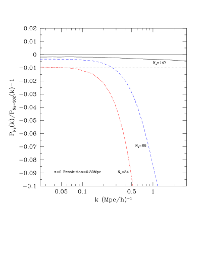
We run a series of C1a simulations that start with the same initial conditions at $z_{\rm init}=100$, have the same force resolution $\Delta x=0.33\,\mbox{$h^{-1}$Mpc}$, and differ only by the time-stepping parameters. Specifically, we run four realisations with box size $1\mbox{$h^{-1}$Gpc}$, $\mbox{$N_{\rm p}$}=1000$ and $\mbox{$N_{\rm g}$}=3000$. The number of time-steps was changing almost by a factor of two from one simulation to another with $\mbox{$N_{\rm s}$}=34,68,147,302$. The two runs with $\mbox{$N_{\rm s}$}=34,68$ have the time-step $\Delta a/a\approx 0.15,0.06$ all the time, while the other two runs have $\Delta a/a$ at $z>3$ limited to $\Delta a/a\approx 0.036,0.015$ for $\mbox{$N_{\rm s}$}=147,302$ correspondingly, and a constant $\Delta a$ at later moments. At $z=0$ they had $\Delta a/a\approx 0.014,0.006$ for $\mbox{$N_{\rm s}$}=147,302$ respectively. For comparison, a run with a constant $\Delta a$, initial $z_{\rm init}=39$, and $\mbox{$N_{\rm s}$}=40$ has $\Delta a/a=0.024$ at $z=0$ and $\Delta a/a\approx 0.1$ at $z=3$.

Figure 10 shows results for the power spectrum of fluctuations relative to the power spectrum of the simulation with the largest number of time-steps $\mbox{$N_{\rm s}$}=302$. There are clearly significant errors in the simulations with the smaller number of steps. Note that the errors are small at long waves which indicates that even a small number of steps is sufficient for tracking the linear growth of fluctuations. However, the errors dramatically increase at small scales because the code cannot keep particles with large velocities inside dense regions. When the number of steps increases the accuracy also improves very substantially, we clearly see converge of the power spectrum when the number of steps increases and becomes $\gtrsim 100$.

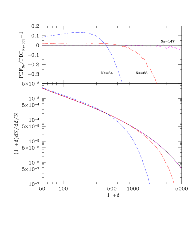
The power spectrum may give somewhat too optimistic impression. After all, even 34 time-steps give an error in $P(k)$ of only 3% at $k\sim 0.3\,h{\rm Mpc}^{-1}$. The problem is that the error is much larger if we look at dense regions. We study this effect by analyzing the density distribution function of dark matter PDF, i.e. the fraction of volume occupied by cells with a given overdensity $\delta$. In order to do that we find the density in each cell of the $3000^{3}$ mesh, and count the number of cells in a given density range $(\delta,\delta+\Delta\delta)$. Figure 11, bottom panel, shows the PDF for those C1a simulations with different number of time-steps. At low densities, the PDF is relatively insensitive to the number of steps, and this is why the errors in $P(k)$ were also reasonable at long-waves. The situation is quite different at large densities: relative errors are very large for densities $\delta>1000$, see top panel in Figure 11. The plot also shows a clear convergence for the simulations with the larger number of steps with very little difference between $\mbox{$N_{\rm s}$}=147$ and $\mbox{$N_{\rm s}$}=302$.

B.2 Effects of force resolution

Figure 12: Effects of force resolution on the power spectrum $P(k)$ at $z=0$ of a series of C1b simulations with the same number of particles $N_{p}=1000^{3}$ and computational box $L=1000\mbox{$h^{-1}$Mpc}$. We run these simulations for grid sizes of $\mbox{$N_{\rm g}$}=$1000, 2000, 3000, and 4000 with the force resolution ranging from $\Delta x=0.25\mbox{$h^{-1}$Mpc}$ to $1\mbox{$h^{-1}$Mpc}$. The plot shows the ratio of the power spectrum $P(k)$ in each simulation to that set-up with the highest resolution run $\mbox{$N_{\rm g}$}=4000$. The dashed-curve is for a simulation with twice larger number of time-steps. With a resolution of $\Delta x=0.5\mbox{$h^{-1}$Mpc}$ the number of steps $\mbox{$N_{\rm s}$}\approx 100$ was sufficient.

Figure 13: Evolution of the power spectrum with redshift for the various C1b simulations. Better force resolution increases the power spectrum, but there are clear indications of convergence at a fixed wavenumber. The simulation with the number of particles equal to the mesh-size (labeled 1 Mpc in the plot) shows disproportionally large suppression of fluctuations at initial stages of evolution.

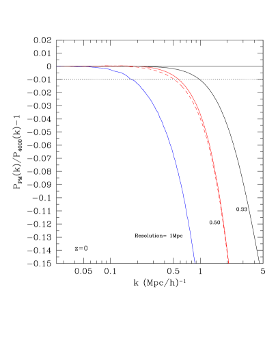
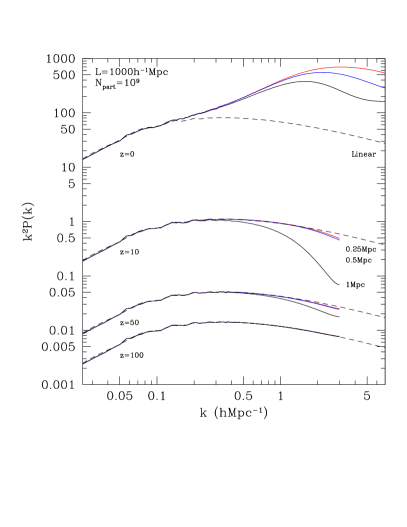
Figures 1 and 2 in the main text show how the power spectrum converges as the force and mass resolution increase. Here we present results of some additional tests. In order to study the effects of the force resolution we run the C1b simulations with the same number of time-steps $\mbox{$N_{\rm s}$}=136$ and number of particles $N_{p}=1000^{3}$, and change the force resolution from $\Delta x=0.25\,\mbox{$h^{-1}$Mpc}$ to $1\,\mbox{$h^{-1}$Mpc}$ by running the same initial conditions using different mesh-sizes. The smallest mesh has the same number of grid points as the the number of particles $N_{g}=N_{p}=1000$. We then run other simulations with $N_{g}=2000^{3},3000^{3}$, and $4000^{3}$ meshes. We also run an additional simulation with $N_{g}=2000^{3}$ but with twice larger time-steps ($\mbox{$N_{\rm s}$}=270$). Figure 12 presents the ratio at $z=0$ of the power spectrum $P(k)$ in each simulation to that with the highest resolution $\mbox{$N_{\rm g}$}=4000$.

Figure 13 shows the evolution of the power spectra (scaled by $k^{2}$ to reduce the dynamical range) in these C1b simulations. Results indicate $\sim 1\%$ convergence for $k\mbox{${\,\hbox{\hbox{$<$}\kern-8.00003pt\lower 4.30554pt\hbox{$\sim$}}\,}$}1\,h{\rm Mpc}^{-1}$. At smaller scales the error increases, but it is still $\sim 20-30\%$ even at $k\approx(3-5)\,h{\rm Mpc}^{-1}$, which is also consistent with what we find from the comparison with the MultiDark simulations in Figure 1 (left panel).

The evolution of the power spectra presented in Figure 13 demonstrates significant suppression of fluctuations for the simulation with the same number of particles and mesh cells $N_{g}=N_{p}=1000$.

References

- Alam et al. (2016) Alam S. et al., 2016, ArXiv e-prints
- Anderson et al. (2012) Anderson L. et al., 2012, MNRAS, 427, 3435
- Baldauf et al. (2016) Baldauf T., Seljak U., Senatore L., Zaldarriaga M., 2016, JCAP, 9, 007
- Bertolini et al. (2016) Bertolini D., Schutz K., Solon M. P., Walsh J. R., Zurek K. M., 2016, Phys. Rev. D, 93, 123505
- Blot et al. (2015) Blot L., Corasaniti P. S., Alimi J.-M., Reverdy V., Rasera Y., 2015, MNRAS, 446, 1756
- Bryan et al. (2014) Bryan G. L. et al., 2014, Rev.Astrn.Astrophys., 211, 19
- Carron et al. (2015) Carron J., Wolk M., Szapudi I., 2015, MNRAS, 453, 450
- Chuang et al. (2015) Chuang C.-H. et al., 2015, MNRAS, 452, 686
- Dawson et al. (2016) Dawson K. S. et al., 2016, AJ, 151, 44
- DESI Collaboration et al. (2016) DESI Collaboration et al., 2016, ArXiv e-prints
- Dodelson & Schneider (2013) Dodelson S., Schneider M. D., 2013, Phys. Rev. D, 88, 063537
- Feng et al. (2016) Feng Y., Chu M.-Y., Seljak U., 2016, ArXiv e-prints
- Gnedin et al. (2011) Gnedin N. Y., Kravtsov A. V., Rudd D. H., 2011, Rev.Astrn.Astrophys., 194, 46
- Habib et al. (2014) Habib S. et al., 2014, ArXiv e-prints
- Heitmann et al. (2009) Heitmann K., Higdon D., White M., Habib S., Williams B. J., Lawrence E., Wagner C., 2009, ApJ, 705, 156
- Hockney & Eastwood (1988) Hockney R. W., Eastwood J. W., 1988, Computer simulation using particles
- Izard et al. (2015) Izard A., Crocce M., Fosalba P., 2015, ArXiv e-prints
- Joachimi (2017) Joachimi B., 2017, MNRAS, 466, L83
- Kitaura & Heß (2013) Kitaura F.-S., Heß S., 2013, MNRAS, 435, L78
- Kitaura et al. (2016) Kitaura F.-S. et al., 2016, MNRAS, 456, 4156
- Klypin & Holtzman (1997) Klypin A., Holtzman J., 1997, ArXiv Astrophysics e-prints
- Klypin et al. (2016) Klypin A., Yepes G., Gottlöber S., Prada F., Heß S., 2016, MNRAS, 457, 4340
- Klypin & Shandarin (1983) Klypin A. A., Shandarin S. F., 1983, MNRAS, 204, 891
- Koda et al. (2016) Koda J., Blake C., Beutler F., Kazin E., Marin F., 2016, MNRAS, 459, 2118
- Kravtsov et al. (1997) Kravtsov A. V., Klypin A. A., Khokhlov A. M., 1997, Rev.Astrn.Astrophys., 111, 73
- Laureijs et al. (2011) Laureijs R. et al., 2011, ArXiv e-prints
- Li et al. (2014) Li Y., Hu W., Takada M., 2014, Phys. Rev. D, 89, 083519
- Mohammed & Seljak (2014) Mohammed I., Seljak U., 2014, MNRAS, 445, 3382
- Mohammed et al. (2016) Mohammed I., Seljak U., Vlah Z., 2016, ArXiv e-prints
- Monaco (2016) Monaco P., 2016, Galaxies, 4, 53
- Neyrinck (2011) Neyrinck M. C., 2011, ApJ, 736, 8
- O’Connell et al. (2016) O’Connell R., Eisenstein D., Vargas M., Ho S., Padmanabhan N., 2016, MNRAS, 462, 2681
- Pearson & Samushia (2016) Pearson D. W., Samushia L., 2016, MNRAS, 457, 993
- Percival et al. (2014) Percival W. J. et al., 2014, MNRAS, 439, 2531
- Pope & Szapudi (2008) Pope A. C., Szapudi I., 2008, MNRAS, 389, 766
- Sánchez et al. (2012) Sánchez A. G. et al., 2012, MNRAS, 425, 415
- Schneider et al. (2016) Schneider A. et al., 2016, JCAP, 4, 047
- Smith et al. (2003) Smith R. E. et al., 2003, MNRAS, 341, 1311
- Springel (2005) Springel V., 2005, MNRAS, 364, 1105
- Swarztrauber (1984) Swarztrauber P., 1984, Parallel Computing, 1, 45
- Takahashi et al. (2009) Takahashi R. et al., 2009, ApJ, 700, 479
- Tassev et al. (2015) Tassev S., Eisenstein D. J., Wandelt B. D., Zaldarriaga M., 2015, ArXiv e-prints
- Tassev et al. (2013) Tassev S., Zaldarriaga M., Eisenstein D. J., 2013, Journal of Cosmology and Astroparticle Physics, 6, 036
- Taylor et al. (2013) Taylor A., Joachimi B., Kitching T., 2013, MNRAS, 432, 1928
- Teyssier (2002) Teyssier R., 2002, Astr.Astrophy., 385, 337
- Wagner et al. (2015) Wagner C., Schmidt F., Chiang C.-T., Komatsu E., 2015, MNRAS, 448, L11
- White et al. (2014) White M., Tinker J. L., McBride C. K., 2014, MNRAS, 437, 2594